Laser Scanning-Aided Virtual Trial Assembly and Assembly Conflict Detection of Welded Box-Type Steel Arch Ribs

Abstract

Physical trial assembly (PTA) of large-scale welded steel structures under complex field conditions still relies on conventional measurement methods such as total stations, making it difficult to continuously capture the boundaries of assembly end-faces and analyze assembly deviations. To address this issue, this study proposes a VTA method based on point cloud data for box-section steel arch ribs, in which end-face boundaries and assembly corner points are extracted to quantitatively evaluate the assembly feasibility between adjacent segments. Based on the extracted assembly features, a VTA framework is further established to perform virtual reconstruction of the spatial assembly poses of welded steel structures and validate structural alignment consistency. Furthermore, the proposed method is validated through an engineering case study. The results demonstrate that the proposed framework can effectively reconstruct the spatial assembly poses of welded box-section steel arch ribs, while enabling quantitative assessment of assembly compatibility and identification of assembly conflicts and weld gap anomalies. Compared with conventional total station-based PTA, the proposed method reduces overall resource consumption and assembly time by approximately 90% and 60%, respectively, demonstrating strong potential for virtual engineering of large-scale steel structures.

1. Introduction

Box-section steel arch ribs are widely used in long-span steel arch bridges and are typically fabricated in segments for on-site welding assembly. To ensure structural alignment and mechanical performance, physical trial assembly (PTA) is generally conducted before erection to verify assembly compatibility and identify potential assembly risks [1]. However, the PTA process is highly resource-intensive and time-consuming, making it increasingly difficult to satisfy the demands of modern bridge construction. Consequently, virtual trial assembly (VTA) has attracted growing attention as an alternative approach for assembly analysis of complex steel structures [2]. Compared with conventional PTA, VTA enables prediction of the final assembly pose of structural components before construction, thereby facilitating early identification of potential assembly risks. While maintaining the required measurement accuracy, VTA can reduce resource requirements by approximately 90% and substantially shorten the trial assembly duration, demonstrating its potential for engineering application [3,4,5].

In recent years, point cloud data have been increasingly applied to quality inspection and deviation analysis of structural components. Compared with conventional measurement methods such as total stations, point cloud data can directly capture continuous three-dimensional surface geometry, making it more suitable for characterizing assembly boundaries and manufacturing deviations [6]. For example, Li et al. [7] conducted quality inspection of precast concrete stairs using point cloud data. Deng et al. [8] achieved automated detection of reinforcement spacing based on three-dimensional keypoints. In addition, Ren et al. [9] quantitatively evaluated manufacturing deviations of steel tower components by integrating measured point clouds with design models through spatial registration.

Building upon these studies, point cloud-based VTA has further enabled the prediction of structural assembly states and the early identification of potential assembly risks through digital alignment of component poses before construction [10]. However, existing studies have mainly focused on prefabricated concrete structures and bolted steel structures. For example, Cheng et al. [11] applied particle swarm optimization (PSO) to derive correction strategies for bolted components. Gu et al. [12] developed a kinematic chain model to investigate error propagation and accumulation in multi-segment bolted structures. Jiang et al. [13] further achieved automated virtual assembly of prefabricated frame structures using extended orthogonal Procrustes analysis (EOPA). Although these methods have achieved promising results, they generally rely on a contact-based assembly assumption, where the optimal assembly state is obtained by minimizing the geometric distance between adjacent components [14]. However, welded assembly requires reserved welding gaps between adjacent segments, making it essentially a gap-constrained non-contact assembly problem. Therefore, existing VTA methods developed under contact-based assumptions cannot directly represent the true assembly state of welded steel arch ribs.

On the other hand, assembly feasibility of welded steel structures is determined by the spatial pose of structural components, geometric matching between adjacent assembly interfaces, and welding gap conditions [15,16,17]. During welded assembly, reserved gaps between adjacent segments must be maintained within an appropriate range [18]. Excessive local gaps may degrade welding quality, whereas insufficient gaps or local contact can lead to assembly interference and additional on-site adjustment. Moreover, local geometric variations near assembly interfaces may alter the spatial distribution of gaps and further affect the final assembly state [19]. Meanwhile, existing VTA studies pay insufficient attention to the global alignment of the assembled structure. For steel arch ribs, small segmental pose errors may accumulate during sequential assembly, ultimately affecting overall alignment. Recent studies have demonstrated that point cloud data can support global geometric analysis of bridge structures, including arch axis extraction and deformation evaluation [20,21]. These findings indicate that point cloud-based methods are capable of bridging local assembly assessment and global structural alignment. Therefore, validation of VTA results from a global perspective is necessary for reliable assembly evaluation of steel arch ribs.

To address the above issues, this study proposes a point cloud-based VTA and assembly risk detection framework for box-section steel arch ribs. First, assembly boundary contours and geometric features are extracted to quantitatively evaluate welding assembly feasibility between adjacent segments. Subsequently, design control coordinates are incorporated into VTA to reconstruct the assembly pose of welded steel arch rib segments in a digital environment. Finally, an overall alignment validation approach based on the assembled arch axis is introduced to evaluate overall validity of VTA results and identify regions with potential assembly anomalies.

2. Methodology

To digitally reconstruct the assembly poses of welded box-section steel arch ribs and identify potential assembly risks, a VTA method based on TLS point clouds is developed. The method consists of three main components: assembly feature extraction, assembly interface compatibility assessment, and virtual trial assembly with assembly risk detection. First, the boundaries and corner points of the assembly end-faces are extracted from the point cloud as geometric features for subsequent VTA (Section 2.1). The extracted end-face features are then used to assess the compatibility between adjacent assembly interfaces (Section 2.2). Finally, the assembly corner points are used to reconstruct the target assembly pose of each segment and to further identify potential assembly risks (Section 2.3).

2.1. Assembly Feature Extraction

2.1.1. End-Face Boundary Extraction and Corner Extraction

During the PTA process, assembly control points for each segment are predefined in the design drawings. These points typically correspond to structural corner points and representative locations along the outer contour, which collectively define the overall geometric shape of the component and serve as references for measurement and positioning. Consequently, reliable identification of these features from scanned data can provide stable geometric references for the VTA process. On this basis, this section presents an end-face feature extraction method for the assembly region. The method involves extracting the end-face boundary and identifying assembly corner points to provide geometric references for subsequent VTA.

End-Face Boundary Extraction

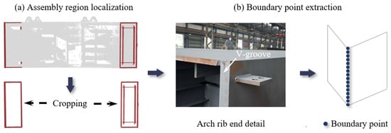
Since steel bridge components are predominantly fabricated by welding steel plates, their scanned point clouds generally exhibit distinct planar characteristics. This structural feature allows the end-face boundary to be determined from the intersection lines of adjacent structural planes. However, steel arch ribs typically contain internal structural elements such as stiffeners and side plates, whose scanned data do not contribute to the extraction of the target assembly boundary. Processing the full point cloud would therefore increase the amount of data involved in subsequent plane segmentation and impose unnecessary computational cost.

Moreover, planar surfaces belonging to these non-target internal structures may be incorrectly identified as target structural planes during iterative segmentation, thereby introducing additional interference into the segmentation process. Spatial cropping is therefore applied to isolate the point cloud around the assembly end, reducing data redundancy and suppressing the influence of these non-target structures before subsequent boundary extraction. RANSAC is subsequently employed to iteratively extract the major structural planes within the cropped assembly region [22]. For the current point set to be segmented, RANSAC determines the supporting points of a candidate plane by comparing the orthogonal distance from each point to the plane. A plane model with sufficient inlier support is then used to estimate the current structural plane, thereby reducing the influence of outliers on plane parameter estimation. For the i-th candidate plane π_i, the plane model is expressed as:

$${\mathit{n}}_i^T\mathit{p}+d_i=0$$

(1)

where n_i denotes the unit normal vector of plane π_i, p is the coordinate vector of a spatial point, and d_i is the plane offset. After extracting the plane with the largest inlier set, its supporting points are removed, and RANSAC is reapplied to the remaining points. The process is repeated until all candidate structural planes within the assembly region have been segmented.

Subsequently, adjacent plane pairs are identified based on the minimum spatial distance between their supporting point sets and the orientation of the plane normals. For any pair of candidate planes π_i and π_j fitted to their respective supporting point sets, the relative orientation is first evaluated from the angle θ_ij (see Equation (2); n_i and n_j denote the unit plane normals) between the corresponding normal vectors, while their spatial proximity is characterized by the minimum distance between their corresponding supporting point sets. Two non-parallel planes are identified as adjacent when this distance is below a predefined threshold. The intersection of an adjacent plane pair represents the theoretical boundary at the assembly end of the steel arch rib. Its direction, l_ij, can be obtained from Equation (3).

$${\theta }_{\mathit{ij}}=\arccos \left(\left|{\mathit{n}}_i^T{\mathit{n}}_j\right|\right)$$

(2)

$${\mathit{l}}_{\mathit{ij}}={\displaystyle \frac{{\mathit{n}}_i\times {\mathit{n}}_j}{‖{\mathit{n}}_i\times {\mathit{n}}_j‖}}$$

(3)

The theoretical boundary provides only the geometric location of the boundary and does not directly represent the discrete samples in the TLS point cloud. Therefore, the original points are searched according to their shortest distances to the theoretical boundary. Points within 0.3 mm are retained as boundary support points, and these points collectively form the measured boundary point set in the original TLS data, as shown in Figure 1.

Figure 1. Boundary extraction based on planar intersections.

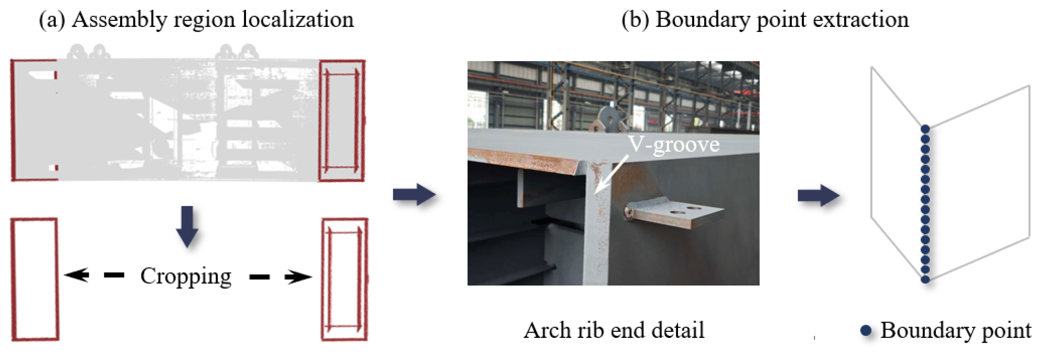
However, in practical scanning, structural occlusion and unfavorable laser incidence angles may result in incomplete data near the assembly end. In such regions, only one of the two adjacent planes forming the V-shaped groove may be sufficiently preserved, preventing the boundary from being determined from their intersection line. To ensure boundary completeness, a projection-based extraction method is further proposed for regions containing only a single planar surface (Figure 2).

Figure 2. Projection-based boundary extraction strategy.

Specifically, in regions where only a single structural plane can be identified, the end-face boundary remains constrained to that plane. The boundary extraction problem can therefore be reduced from a three-dimensional search to two-dimensional contour extraction in the local plane. Principal component analysis (PCA) is first employed to estimate the principal directions of the local point cloud [23]. For a local point set containing (N) points, its covariance matrix C is defined as:

$$C={\displaystyle \frac{1}{N}}{\sum }_{k=1}^N\left(p_k-\overline{p}\right){\left(p_k-\overline{p}\right)}^T$$

(4)

Here, p_k denotes the k-th 3D point, and $\overline{p}$ is the centroid of the local point set. After eigendecomposition of C, the eigenvectors corresponding to the two largest eigenvalues define the in-plane principal directions, while that associated with the smallest eigenvalue estimates the local plane normal. These two principal directions are used to construct a local 2D coordinate system, onto which the 3D points are projected. This transformation reduces the boundary extraction problem to two dimensions while preserving the relative in-plane geometry of the original points. An initial boundary candidate is subsequently identified using the Alpha Shape (α-shape) algorithm.

The α-shape algorithm constructs boundaries based on global topology and is therefore sensitive to local point density variations and boundary ambiguity [24]. This may lead to the inclusion of nonphysical boundary points, while internal spurious boundaries may also be retained in regions with complex defects [25]. To improve boundary identification accuracy, a secondary filtering strategy based on local angular variation is adopted. The extracted contour points are first mapped back onto the projected point set for local neighborhood verification. For each candidate point, all neighboring points (N_p) within a predefined radius (r) are retrieved to form a local neighborhood. For cases where N_p is less than or equal to three, the point is treated as a sparse or noisy point and removed. For valid points, adjacent vectors are constructed from the local neighborhood, and the angular variation between consecutive vectors is computed. The maximum angle, denoted as θ_max, is then recorded. The point is identified as a boundary point if θ_max is greater than the threshold (θ_thr); otherwise, it is considered an interior point and excluded. Algorithm 1 summarizes the boundary extraction procedure for incomplete V-groove regions with one missing side.

Algorithm 1. Boundary extraction for incomplete V-groove regions

Input:  Point cloud of single-surface region, Qs;  Search radius r;  Angular threshold θthr;  Alpha-shape parameter α; Output:  Boundary point set – B  (R,qc) = PCA (Qs);  Q2D = Projection of Qs onto the local plane;  B0 = AlphaShape (Q2D,α);  B = ∅;  for i = 1 to |B0| do    pi = B0(i);    Np = {q ∈ Q2D‖q − pi‖) ≤ r};    if |Np| ≤ 3 then     skip current point;    end if    θmax = 0;    for each adjacent vector pair do     compute angular variation θ;     if θ > θmax then      θmax = θ     end if    end for    if θmax > θthr then     B = B ∪ {pi};    end if  end for  return B

After the reliable 2D boundary points are obtained, an inverse coordinate transformation is applied to recover their positions in the original 3D space. RANSAC is then employed to fit straight lines to the reconstructed 3D boundary points. The fitted boundary segments are subsequently combined with those obtained from the two-plane intersection method to form the complete end-face boundary.

Corner Point Detection

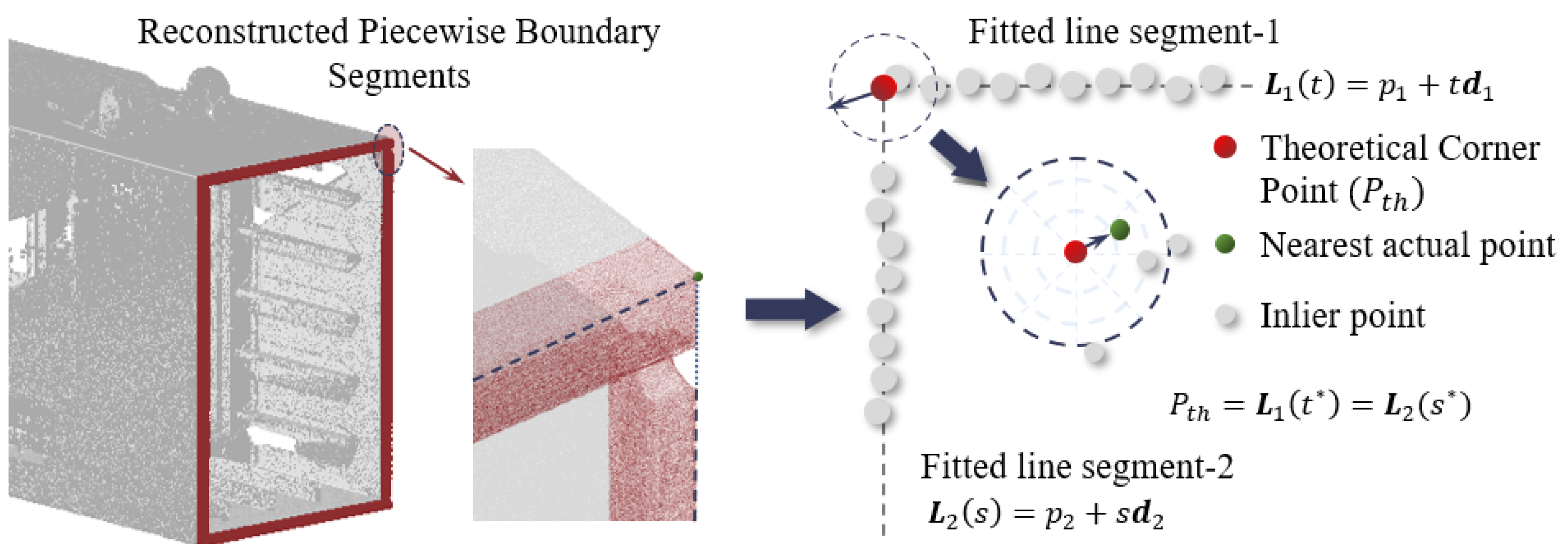
After extracting the boundary of the assembly region, the corner points of the end-section of the steel arch rib are further identified. Geometrically, a corner is defined by the intersection of two adjacent boundary segments. Therefore, the theoretical corner point (P_th) is first determined from the parametric equations of the two fitted boundary lines, as shown in Figure 3. This analytically derived intersection represents the geometric location of the corner. The nearest point to the theoretical corner is then identified in the original point cloud and taken as the corresponding actual corner point, thereby completing the corner localization.

Figure 3. Assembly corner identification strategy (p_i: line reference point; d_i: line direction vector; t and s: line parameters).

Accuracy Test

To validate the accuracy of the proposed end-face feature extraction method, a series of numerical simulations were conducted. In contrast to field-measured data, numerical simulation enables precise control over both the geometric model and the point cloud generation process, thereby effectively eliminating the influence of manufacturing and measurement uncertainties.

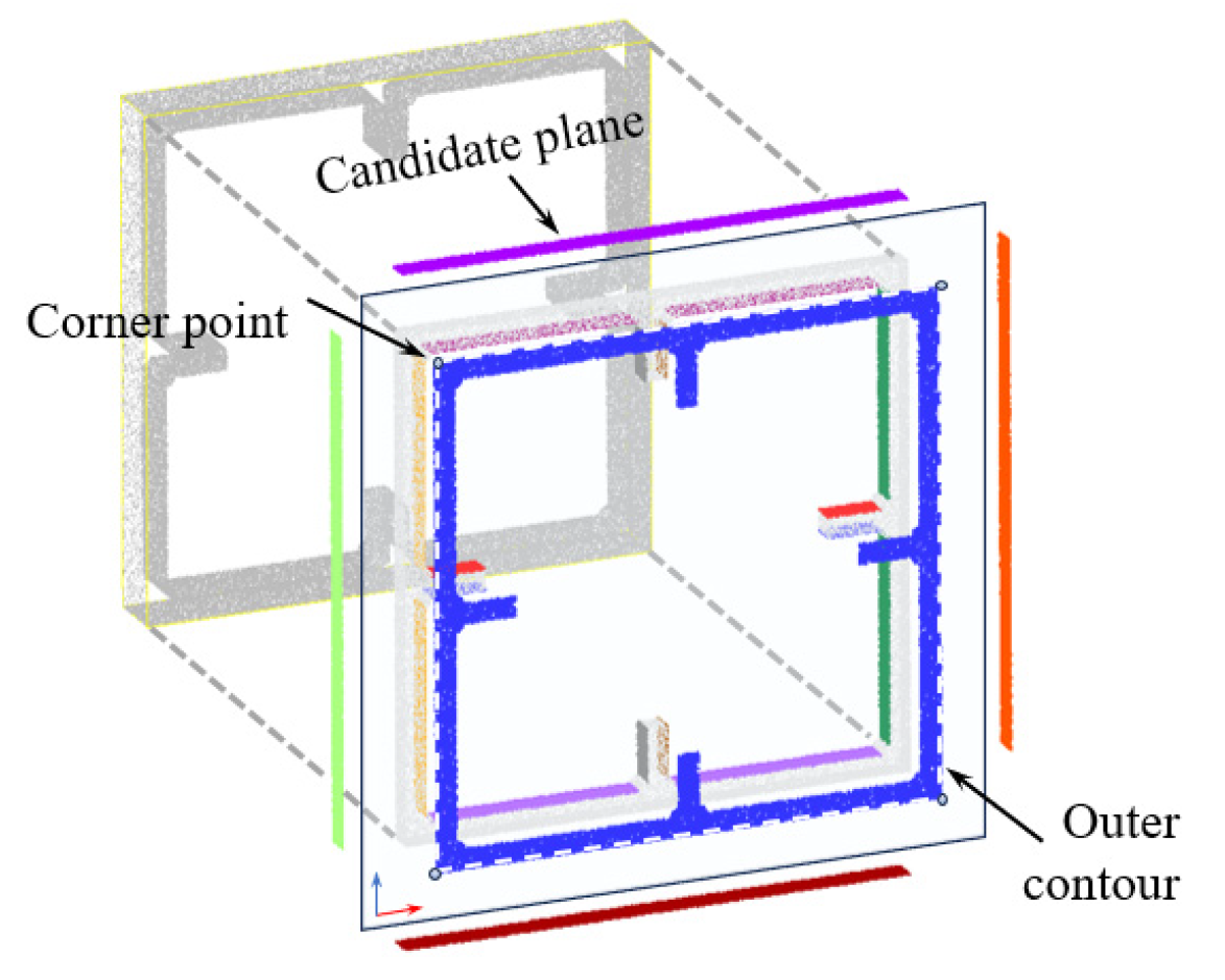
First, a standard end-face model with explicitly defined geometric parameters is constructed (Figure 4), in which both the boundary contour and corner coordinates are known exactly. A rigid transformation is subsequently applied to normalize the model pose by constraining the target end-face to the XOZ plane and aligning one corner with the coordinate origin, thereby establishing a unified spatial reference framework for subsequent accuracy evaluation of the extracted corner points. After pose alignment, random discrete sampling is performed over the end-face region to generate a standard point cloud model. To account for data incompleteness caused by occlusion or limited incidence angles in practical scanning, three representative scenarios are considered, namely complete data, single-side missing, and double-side missing. In the single-side missing scenario, points on one side of the end-face are removed, whereas in the double-side missing scenario, two non-adjacent sides are simultaneously removed to mimic the absence of both upper and lower surfaces in field scanning of large-scale components. Furthermore, point cloud datasets with varying sampling densities are generated to analyze the influence of point distribution characteristics on feature extraction accuracy. The point cloud density is defined as:

$$\rho ={\displaystyle \frac{n_{\mathit{pcd}}}{{\displaystyle \sum _{i=1}^D{A}_i}}}$$

(5)

where ρ denotes the point cloud density, n_pcd is the number of points, A_i is the area of each constituent surface, and D is the number of planes forming the end-face. Under varying point cloud densities and data-missing conditions, the proposed method is applied to extract end-face boundaries and corner points. The extracted corner coordinates are compared with their exact counterparts, with the Euclidean distance used as the accuracy metric. The mean error is defined as the average localization error of the eight corners in each test case, while the standard deviation characterizes the dispersion of the corresponding corner localization errors. The results are summarized in Table 1.

Figure 4. Standard end-face model for numerical simulation.

Table 1. Corner extraction errors under varying point cloud densities and data incompleteness.

Point Cloud Density (ρ/mm−2)	Data Missing Condition	Mean Error (mm)	Maximum Error (mm)	Standard Deviation (mm)
15	Complete data	0.154	0.170	0.0166
	Single-side missing	0.169	0.188	0.0153
	Double-side missing	0.182	0.194	0.0121
30	Complete data	0.137	0.150	0.0124
	Single-side missing	0.156	0.177	0.0195
	Double-side missing	0.161	0.181	0.0159
45	Complete data	0.116	0.139	0.0206
	Single-side missing	0.128	0.151	0.0207
	Double-side missing	0.155	0.174	0.019
60	Complete data	0.073	0.096	0.0216
	Single-side missing	0.095	0.112	0.0146
	Double-side missing	0.125	0.146	0.021

The results show that both point cloud density and data completeness have a clear influence on corner localization accuracy. Under the complete-data condition, as the point cloud density increases from 15 mm⁻² to 60 mm⁻², the mean error decreases from 0.154 mm to 0.073 mm, while the maximum error decreases from 0.170 mm to 0.096 mm, corresponding to reductions of approximately 52.6% and 43.5%, respectively. The single-side-missing and double-side-missing conditions exhibit the same overall trend. These results indicate that higher point cloud density increases the number of effective samples along the end-face boundary, providing more stable support for boundary fitting and thereby reducing corner localization errors.

Data completeness also affects corner localization accuracy. At a given point cloud density, both the mean and maximum errors increase with the extent of missing data. For example, at ρ = 45 mm⁻², the mean errors under the complete-data, single-side-missing, and double-side-missing conditions are 0.116, 0.128, and 0.155 mm, respectively, while the corresponding maximum errors are 0.139, 0.151, and 0.174 mm. This trend can be attributed primarily to the increasing extent of missing data. As the missing region expands, some boundary segments can no longer be determined directly from the intersections of adjacent planes and must instead be recovered using single-plane projection. Since these recovered boundaries are constrained by only one structural plane, less geometric information is available to determine the boundary direction and corner position. Corner localization therefore becomes more dependent on the fitting accuracy of the recovered boundaries, resulting in larger errors under the double-side-missing condition.

Overall, point cloud density and data completeness both affect corner localization accuracy. Lower point cloud density reduces the number of samples available around the end-face boundary, which limits the information available for boundary fitting and increases localization error. Missing data further reduces the completeness of the sampled boundary and decreases the information available for determining the boundary direction and corner position. Nevertheless, the maximum error remains below 0.20 mm in all test cases, satisfying typical engineering tolerance requirements and indicating stable performance under incomplete point cloud conditions.

2.2. Assembly Interface Compatibility Assessment

In VTA, geometric differences between adjacent segment end-sections may result in weld gaps outside the allowable range or local boundary offsets at the joint even after pose alignment, necessitating an assessment of end-section compatibility. For welded box-type sections, compatibility is evaluated at multiple levels, including global dimensions, sectional shape, and local boundary matching. We define a composite mismatch index that combines the corresponding mismatch measures to quantify the mismatch between adjacent end-sections.

2.2.1. Global Dimensional Consistency

To ensure stability and comparability, the raw boundary point set is first standardized before evaluating global dimensional consistency. Principal component analysis (PCA) is used to extract principal directions and establish a local 2D coordinate system, onto which the points are orthogonally projected to obtain a planar contour. As the boundary points are coplanar, this step does not introduce geometric distortion. The contour is then divided into four segments based on corner connectivity, with each segment fitted by a straight line to obtain a stable representation. According to relevant specifications, area deviation and diagonal length difference are used to quantify global dimensional inconsistency [26].

Area Deviation

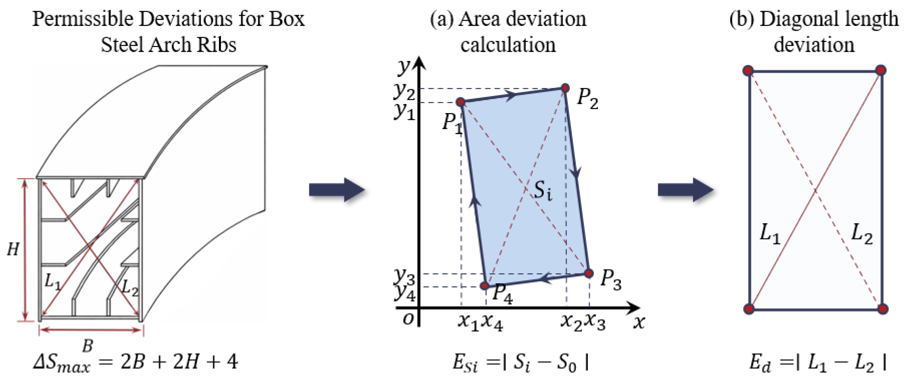
Manufacturing deviations in steel arch ribs may alter the positions of the end-face corners, causing the four corners to deviate from an ideal rectangular configuration. Therefore, estimating the end-face area simply from the measured width and height may not accurately represent its actual geometry. Instead, the end-face area is computed directly from the four extracted corner points, P_i = (x_i, y_i), i = 1, …, 4. With the four corners ordered clockwise along the boundary, the area S_i of the i th measured end-face is calculated as follows:

$$S_i={\displaystyle \frac{1}{2}}\left|x_1{y}_2+x_2{y}_3+x_3{y}_4+x_4{y}_1-y_1{x}_2-y_2{x}_3-y_3{x}_4-y_4{x}_1\right|$$

(6)

After obtaining the measured end-face area S_i, a design reference area is required to quantify the difference between the measured and designed end-faces. The reference area of the designed end-face is calculated from the design width (B) and height (H) as (Figure 5). Accordingly, the area deviation of the i th measured end-face is defined as E_s,i = |S_i − S₀|. Considering that both B and H are allowed to vary within ±2 mm during fabrication, the effects of dimensional tolerances on the area variation are further analyzed. Let δ_B and δ_H denote the deviations of the actual width and height from their design values, respectively. The actual dimensions under manufacturing tolerances can then be expressed as B + δ_B and H + δ_H. By subtracting the designed area BH from the area calculated using the tolerance-adjusted dimensions (B + δ_B)(H + δ_H), the area variation induced by dimensional deviations can be obtained, as given in Equation (7).

∆S = Hδ_B + δ_HB + δ_Bδ_H

(7)

where Hδ_B and δ_HB represent the contributions of width and height deviations to the area variation, respectively, and δ_Bδ_H denotes the cross term caused by the simultaneous occurrence of the two-dimensional deviations. Since both the width and height tolerances are ±2 mm and ∆S increases monotonically with δ_B and δ_H within this range, the maximum area deviation occurs when δ_B = δ_H = 2 mm. The upper bound of the area deviation can therefore be expressed as:

∆S_max = 2H + 2B + 4 (mm²)

(8)

Figure 5. Reference model for global dimensional evaluation.

To quantitatively evaluate the measured area deviation relative to the allowable fabrication range, the maximum allowable area deviation ∆S_max is used as the normalization reference. The normalized area deviation of the i th end-face, ${\tilde{E}}_{S,i}$, is defined as:

$${\tilde{E}}_{S,i}={\displaystyle \frac{E_{s,i}}{\Delta S_{\mathit{max}}}}$$

(9)

When ${\tilde{E}}_{S,i}$ approaches zero, the difference between the measured and designed end-face areas is relatively small. When ${\tilde{E}}_{S,i}$ exceeds 1, the measured area deviation surpasses the allowable limit.

Diagonal Length Deviation

For an ideal rectangular end-section, the two diagonal lengths should be equal, and their deviation can therefore reflect changes in the end-face shape. For the extracted boundary, the diagonal lengths calculated from the corner coordinates are denoted as L₁ and L₂, respectively. Their difference is defined as:

E_d,i = |L₁ − L₂|

(10)

To enable consistent comparison across components, the diagonal length deviation is further normalized. For box-type steel arch ribs, the allowable limit is specified as d_lim = 4 mm. The normalized diagonal deviation, denoted as ${\tilde{E}}_{d,i}$, is defined in Equation (12). This metric characterizes the deviation of the end-section from rectangular symmetry. Values of ${\tilde{E}}_{d,i}\le 1$ indicate that the deviation satisfies the allowable tolerance, whereas values exceeding 1 indicate that the deviation exceeds the specified limit.

$${\tilde{E}}_{d,i}={\displaystyle \frac{\left|L_1-L_2\right|}{4}}$$

(11)

2.2.2. Local Boundary Matching

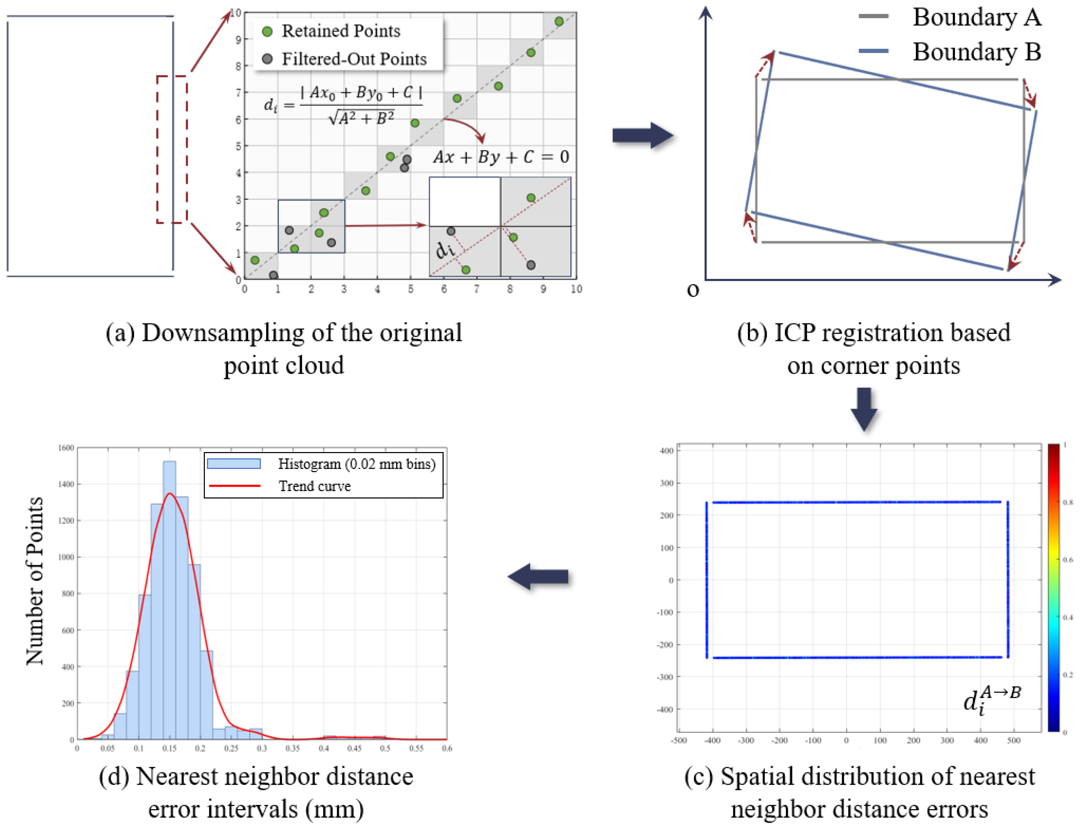
Boundary matching between two assembly end-sections is quantified using nearest-neighbor distances. However, inconsistencies in local point density across the boundary points may introduce bias into the evaluation, thereby misrepresenting the actual geometric deviation. To mitigate this effect, a uniform down-sampling step is applied prior to distance computation [27].

As illustrated in Figure 6, a regular grid with fixed resolution is constructed in the two-dimensional projection plane, and both boundary point sets are mapped to the corresponding grid cells. For cells containing corner points, the corner points are directly retained to preserve key geometric features of the contour. For cells containing only a single boundary point, that point is retained to avoid information loss. For cells containing multiple boundary points, the point with the minimum distance to the fitted line of the associated boundary segment is selected as the representative point.

Figure 6. Local boundary matching and deviation evaluation.

This procedure improves nearest-neighbor distance evaluation while preserving boundary integrity and corner features. Using four pairs of corresponding corner points as constraints, the assembly end-sections are aligned via the ICP algorithm [28], followed by bidirectional distance computation (A→B and B→A). Let the registered contour point sets of end-sections A and B be denoted as ${\left\{p_i\right\}}_{i=1}^N$ and ${\left\{q_i\right\}}_{i=1}^N$, respectively. The bidirectional nearest-neighbor distances are defined as follows:

$$\begin{array}{l}{d}_i^{A\to B}={\min }_{1\le j\le M}‖p_i-q_j‖\\ d_j^{B\to A}={\min }_{1\le i\le N}‖q_j-p_i‖\end{array}$$

(12)

Since contour matching is governed by the maximum local geometric discrepancy, and the retained points after denoising and boundary extraction represent the true boundary, the maximum value among the bidirectional nearest-neighbor distances is adopted as the contour matching error, defined as:

$$D_{\max }=\max \left({\max }_{1\le i\le N}{d}_i^{A\to B},\hspace{1em}{\max }_{1\le j\le M}{d}_j^{B\to A}\right)$$

(13)

The distance-based contour discrepancy between assembly end-sections corresponds to the misalignment encountered during assembly. According to the specification, the allowable misalignment between mating components is limited to D_lim = 1 mm. Based on this criterion, a normalized contour matching error, denoted as ${\tilde{E}}_{c,\mathit{ij}}$ (Equation (14)), is defined. Values of ${\tilde{E}}_{c,\mathit{ij}}\le 1$ indicate that all local discrepancies remain within the allowable tolerance, whereas ${\tilde{E}}_{c,\mathit{ij}}>1$ indicates that at least one location exceeds the specified limit.

$${\tilde{E}}_{c,\mathit{ij}}={\displaystyle \frac{D_{\mathit{max}}}{D_{\mathit{lim}}}}$$

(14)

2.2.3. Composite Mismatch Index

To quantify the geometric compatibility between adjacent assembly end-sections T_i and T_j, a composite mismatch index J_T,ij is constructed from the normalized metrics ${\tilde{E}}_{S,i}$, ${\tilde{E}}_{d,i}$, and ${\tilde{E}}_{C,\mathit{ij}}$. It should be noted that the area deviation and diagonal length deviation are originally defined for individual end-sections. To ensure consistency in the evaluation hierarchy and to reflect the worst-case assembly condition, these metrics are extended to the segment-pair level by taking the maximum value between two adjacent sections, defined as:

$$\begin{gathered} {\tilde{E}}_{S,\mathit{ij}}=\max \left({\tilde{E}}_{S,i},{\tilde{E}}_{S,j}\right) \\ {\tilde{E}}_{d,\mathit{ij}}=\mathit{max}({\tilde{E}}_{d,i},{\tilde{E}}_{d,j}) \end{gathered}$$

(15)

Accordingly, the composite mismatch index is given by Equation (16), where ${\tilde{E}}_{S,\mathit{ij}}$ and ${\tilde{E}}_{d,\mathit{ij}}$ denote the area deviation and diagonal length deviation evaluated at the segment-pair level, respectively.

$$J_{T,\mathit{ij}}=w_1{\tilde{E}}_{S,\mathit{ij}}+w_2{\tilde{E}}_{d,\mathit{ij}}+w_3{\tilde{E}}_{C,\mathit{ij}}$$

(16)

Here, w₁, w₂, and w₃ denote the weighting coefficients associated with the area error, diagonal length error, and boundary matching error, respectively, subject to w₁ + w₂ + w₃ = 1. Since the boundary matching error ${\tilde{E}}_C$ directly reflects assembly misalignment and plays a dominant role in assembly feasibility evaluation, it is assigned a larger weight. Accordingly, the coefficients are set to w₁ = 0.25, w₂ = 0.25, and w₃ = 0.5. Since all error metrics are normalized by their allowable limits and the weights sum to unity, the composite index J_T,ij ≤ has a clear physical meaning. Specifically, J_T,ij ≤ 1 indicates that the composite mismatch index is within the defined threshold. Nevertheless, assembly feasibility requires each individual normalized error metric to be less than or equal to 1, and all individual error metrics must satisfy their respective allowable limits.

2.3. Assembly Risk Detection

2.3.1. Virtual Trial Assembly

During PTA, the spatial pose of each segment is constrained by control points defined in the design model. Therefore, in VTA, the corresponding design control points and extracted corner points from the measured segment are matched to determine the rigid transformation between the two coordinate systems. The measured segment is then transformed into the design coordinate system for subsequent assembly evaluation. Based on this transformation, the assembly state can be evaluated by calculating the spatial distances between the corresponding design control points and the transformed measured corner points. In addition, a prescribed gap must be maintained between adjacent segments to satisfy welding requirements. In the proposed VTA framework, this gap constraint is defined as the Euclidean distance between corresponding corner points on adjacent end-faces.

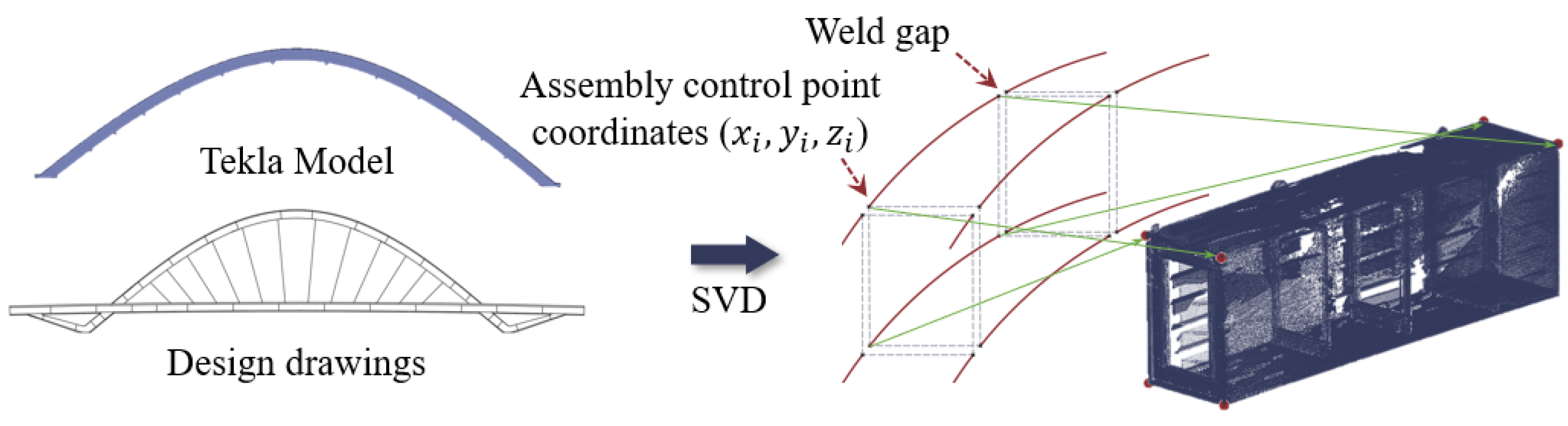
After establishing the correspondence between the extracted assembly corner points and design control points, the spatial pose of each segment is reconstructed through rigid transformation. Specifically, the pose reconstruction problem is formulated as a rigid registration problem, where the optimal rotation matrix R and translation vector t are solved to recover the target assembly state.

The centroids of the two corresponding point sets are first calculated, and each point set is centralized by subtracting its centroid. This operation removes the translational component and converts the registration problem into a rotation estimation problem. A covariance matrix is subsequently constructed, and under the orthogonality constraint R^TR = I, the optimal rotation matrix is obtained using singular value decomposition (SVD) [29]. The translation vector is then calculated according to the centroid relationship after rotation estimation, yielding the complete rigid transformation between the measured model and the target assembly state (Figure 7).

Figure 7. SVD-based rigid transformation for VTA pose reconstruction.

2.3.2. VTA Result Validation

Due to the high sensitivity of the arch axis to segment pose deviations, even the transformation error of a single segment may induce a global deviation in the arch rib alignment, thereby affecting the reliability of subsequent conflict analysis. Therefore, following SVD-based pose estimation, the VTA results are further validated by comparing the arch axis reconstructed after VTA with the design arch axis. Since the bottom surface of the steel arch rib maintains a stable geometric correspondence with the design arch axis, the validation is performed by analyzing the spatial deviation of the transformed bottom surface relative to the design reference.

Specifically, the bottom surface of the design model is adopted as the reference surface. To reduce the influence of discretization in the reference model, the average point spacing of the measured bottom surface point cloud is first computed, after which the design bottom surface is uniformly resampled with a smaller point spacing to better approximate a continuous geometric representation. Subsequently, the transformed bottom surface after VTA is compared with the reference surface through nearest-neighbor distance analysis [30]. For each point on the transformed bottom surface, the nearest-neighbor distance to the design bottom surface is computed, forming a spatial deviation field relative to the design state. The resulting deviation field is further mapped onto the reference surface for visualization and used to assess the reliability of the VTA results.

2.3.3. Assembly Conflict Detection

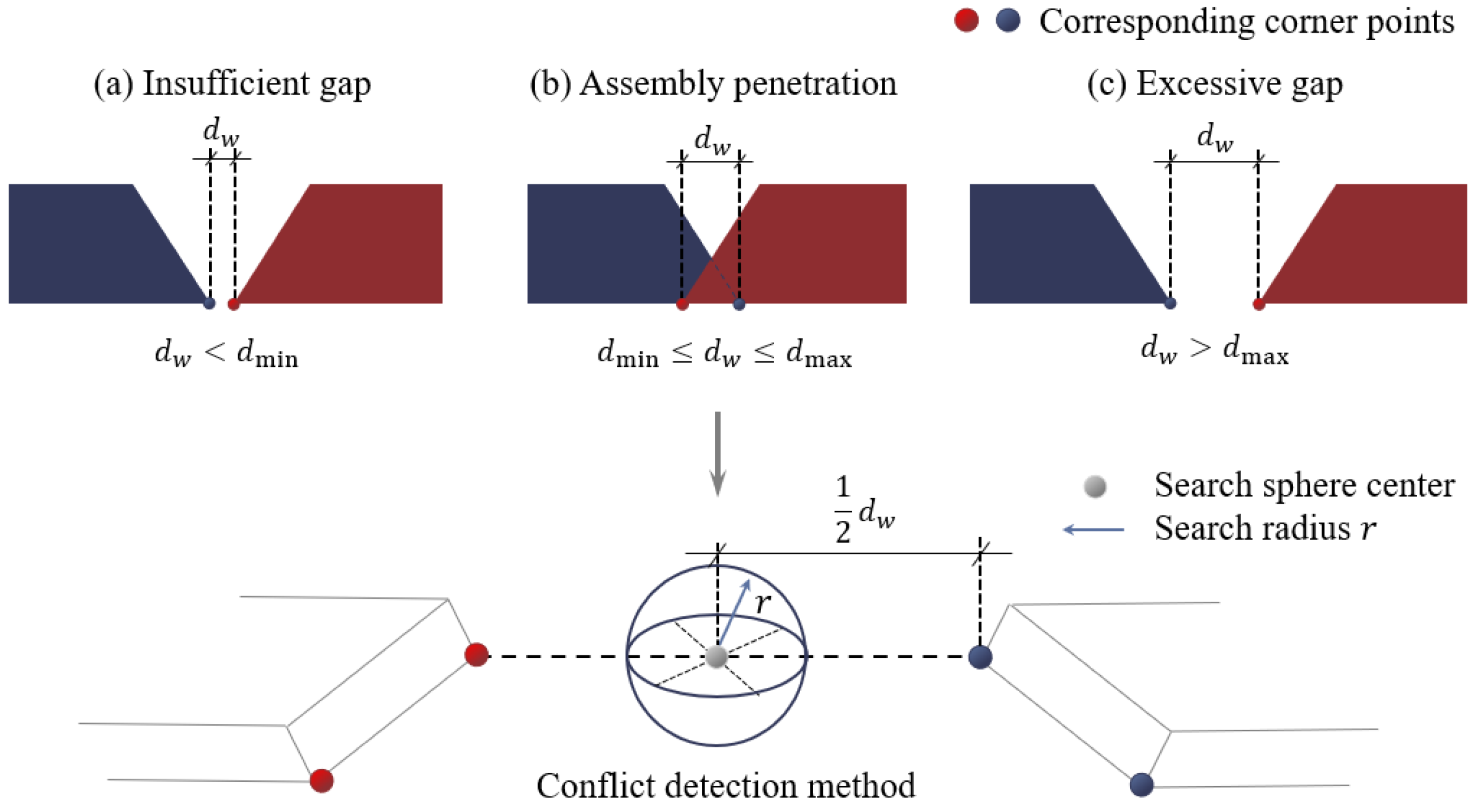
Based on the weld gap distribution and local overlap conditions after VTA, assembly conflicts can be categorized into three types. The first corresponds to assembly interference, where pose deviations or manufacturing errors lead to local spatial overlap between adjacent segments, representing the most critical form of assembly conflict. In addition, weld seam gaps that are either undersized or oversized also constitute assembly conflicts, as both conditions adversely affect welding quality and the structural performance of the assembled system.

To detect the three types of assembly conflicts described above, the distances between corresponding corner points on adjacent mating faces are first evaluated. Let a_i and b_i denote the three-dimensional coordinates of the i-th pair of corresponding corner points. The weld gap is then calculated as the Euclidean distance $d_{w,i}={‖{\mathit{a}}_{\mathit{i}}-{\mathit{b}}_{\mathit{i}}‖}_2$. If the calculated weld gap falls outside the allowable range [d_min,d_max], then an assembly deviation is identified. For corner pairs with weld gaps within the allowable range, an additional interference check is performed to identify potential spatial overlap between adjacent segments. Specifically, a spherical detection region is constructed with its center at the midpoint of a_i and b_i and a radius of ${\displaystyle \frac{1}{2}}{d}_{w,i}$, placing both corner points on the sphere. If the region contains other surface sampling points, then potential assembly interference is identified; otherwise, the local joint is considered to satisfy the specified gap and interference criteria (Figure 8).

Figure 8. Weld gap-based assembly conflict detection framework.

3. Case Study and Discussion

3.1. Project Background

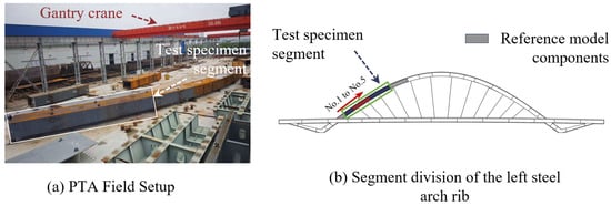
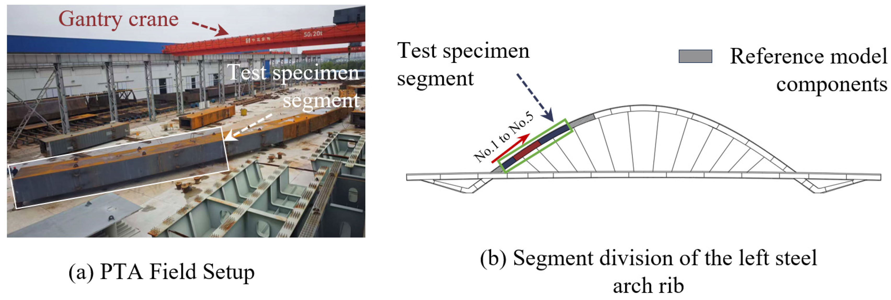
To validate the applicability of the proposed method, point cloud acquisition and VTA-based assembly risk assessment were conducted on selected segments of a box-type steel arch rib. The investigated bridge has a main span of approximately 166 m, with a maximum segment length of 16 m. The box section is 2 m wide and 3 m high (Figure 9). In conventional fabrication practice, PTA of a single side steel arch rib typically requires approximately two weeks and involves extensive use of transport vehicles, gantry cranes, and multiple construction crews. Moreover, the discrete measurements obtained during PTA cannot fully characterize the overall structural alignment. In this study, three measured arch rib segments were selected for validation, while two standard models with zero geometric error, corresponding to Segments No. 1 and No. 5 at both ends of the assembly, were adopted to establish the reference for assembly evaluation.

Figure 9. Project overview of the VTA test case.

Point cloud data were acquired using a Z+F IMAGER 5010C terrestrial laser scanner (Zoller + Fröhlich GmbH, Wangen im Allgäu, Germany), which exhibits low range noise of 0.2 mm at distances within 25 m. Six scan stations were established to capture the structural geometry from different viewpoints. Two angular resolutions of 0.009° and 0.0036° were adopted for different scanning tasks. Initially, the entire scene was scanned at a resolution of 0.009° to obtain the overall spatial information and identify the target structural components while reducing acquisition time. Subsequently, high-resolution scanning at 0.0036° was performed on the steel arch rib segments and their key geometric feature regions, particularly the assembly end-faces and boundaries, to obtain detailed geometric information for subsequent feature extraction and VTA analysis.

3.2. Geometric Compatibility Results of Assembly Interfaces

The compatibility of the assembly interfaces between adjacent segments in the VTA tests was evaluated using the method described in Section 2.2.1, and the results are presented in Table 2. All evaluation metrics remained within the allowable limits, with a maximum composite mismatch index of 0.379.

Table 2. Pre-assembly matching assessment results for adjacent end-sections.

Inspection Location	${\tilde{\mathit{E}}}_{\mathit{S},\mathit{ij}}$	${\tilde{\mathit{E}}}_{\mathit{d},\mathit{ij}}$	${\tilde{\mathit{E}}}_{\mathit{C}}$	${\mathit{J}}_{\mathit{T,ij}}$
No. 1–No. 2	0.104	0.025	0.195	0.13
No. 2–No. 3	0.066	0.065	0.281	0.173
No. 3–No. 4	0.131	0.22	0.582	0.379
No. 4–No. 5	0.085	0.158	0.63	0.376

Further comparison across the inspection locations shows that larger diagonal length deviations, boundary matching deviations, and composite mismatch indices occur mainly at No. 3–No. 4 and No. 4–No. 5. The normalized diagonal length deviations at these two locations are 0.220 and 0.158, respectively, approximately 3.38 and 2.43 times the maximum recorded at the first two locations. Their normalized boundary matching deviations are also more than twice the corresponding maximum. In contrast, the area deviation does not exhibit a similar increase. At No. 4–No. 5, the value is only 0.085, lower than the 0.104 recorded at No. 1–No. 2. These differences indicate that the assembly deviations at No. 3–No. 4 and No. 4–No. 5 are not primarily associated with changes in the overall cross-sectional area but are mainly reflected in end-face shape differences and local boundary mismatch. Accordingly, Segment No. 4 should be closely monitored during field erection, and both interfaces connecting it to the adjacent segments should be carefully verified. These results demonstrate that the proposed pre-assembly assessment therefore provides more than a check against allowable limits; comparison of the individual metrics also helps locate the main mismatches and characterize their geometric form.

3.3. Analysis of VTA Results

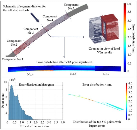
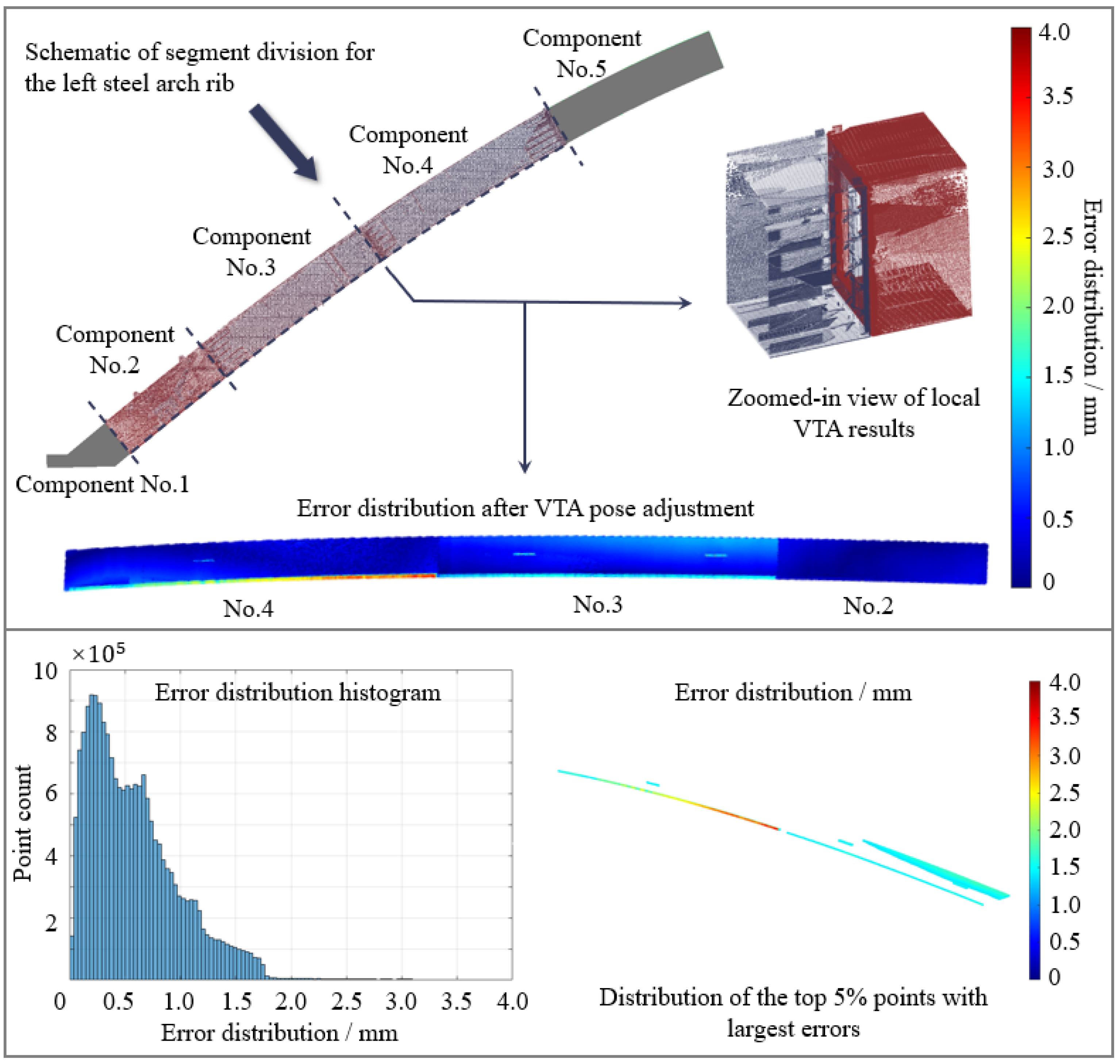
Figure 10 shows the deviation distribution of each segment relative to the designed arch axis after VTA pose adjustment. All deviations remain within the allowable limits specified by relevant standards, indicating that the alignment of the assembled segments satisfies the design requirements. The error histogram further shows that most deviations are concentrated within 2 mm and follow a smooth and continuous distribution, indicating good geometric consistency between segments at the global scale. Analysis of the top 5% highest deviation points reveals that high-deviation regions occupy only a small proportion of the overall distribution and are mainly concentrated near one side boundary of Segment No. 4. These results demonstrate that the proposed VTA method can effectively correct the overall spatial pose of box-section steel arch ribs, such that the remaining assembly deviations are primarily manifested as local geometric discrepancies.

Figure 10. VTA results for the steel arch rib.

From the perspective of error formation, the observed deviations mainly originate from incomplete local contour representation caused by scanning occlusion rather than inaccurate spatial alignment between arch rib segments. In the proposed VTA procedure, each segment is independently transformed as a rigid body, preventing local geometric deviations from propagating or accumulating during successive assembly. Consequently, the reconstructed assembly state still provides a reliable representation of the overall assembly condition and supports subsequent assembly risk analysis. This non-accumulative error characteristic is particularly important for assembled steel structures, where cumulative deviations may eventually result in global assembly misalignment.

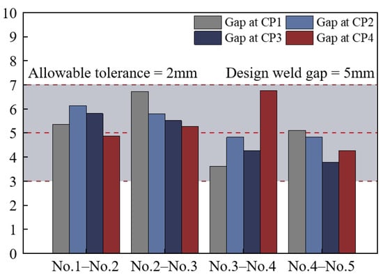
Combined with the assembly gap analysis results (Figure 11), the potential assembly issues of the box-section steel arch rib can be further evaluated. The results indicate that, with the overall structural alignment satisfying the design requirements, the welding gaps between the three segment pairs all satisfy the specified welding gap requirements, and no local spatial interference is observed. This suggests that the manufacturing deviations of the current segments are insufficient to affect proper assembly.

Figure 11. Assembly conflict identification results after VTA.

From an engineering application perspective, the obtained VTA results can be used to identify high-risk assembly regions in advance and provide early warning and decision support for field assembly operations, thereby reducing the risk of rework. In terms of economic efficiency, point cloud data acquisition required approximately 4 h, while point cloud preprocessing and VTA analysis were completed within 3 h using three computers equipped with Intel i5-14600KF processors. In contrast, conventional PTA of the same three steel arch rib segments requires multiple operations, including ground layout, gantry crane-assisted transportation, manual measurement, and alignment adjustment, involving dozens of workers and taking approximately 18 h (2.5 working days). Accordingly, the proposed VTA method reduces pre-assembly resource requirements by approximately 90% and shortens the pre-assembly duration by approximately 60%, further demonstrating its potential for assembly state assessment of steel structures.

4. Conclusions

This study proposes a point cloud-based VTA method for assembly risk detection of box-section steel arch ribs. The main conclusions are summarized as follows:

(1)

An end-face boundary extraction method combining plane intersection line analysis and projection-based boundary extraction is proposed, enabling reliable extraction of assembly features under conditions of incomplete local point cloud data.

(2)

A quantitative evaluation method for assembly interface compatibility is established based on multi-level geometric constraints and a normalized composite mismatch index. In addition, segment assembly risks are formulated as corner point gap constraint problems, enabling assessment of both assembly feasibility and post-assembly structural alignment.

(3)

The engineering case study demonstrates that the proposed VTA method can effectively identify potential assembly risks while maintaining the overall structural alignment, thereby providing a reliable geometric basis for field construction.

References

- Wan, P.-J.; Chen, Z.; Ye, X.-P.; Xia, Q.; Xu, Y.; Zhang, J. Virtual pre-assembly method for bridge tower crossbeam lifting based on temperature effect analysis and 3D laser scanning technology. Adv. Struct. Eng. 2025, 28, 2910–2924. [Google Scholar] [CrossRef] [Scilit]
- Xu, C.; Xiong, W.; Zhu, Y.; Cai, C.S. A point cloud virtual trial assembly method for preventive quality control of prefabricated bridge. Struct. Control Health Monit. 2025, 2025, 8861887. [Google Scholar] [CrossRef] [Scilit]
- Cao, Z.; Xu, Y.; Li, W.; Xia, Q.; Zhang, J. 3D virtual closure assembly for a cable-stayed bridge via partial point cloud registration. Autom. Constr. 2026, 187, 106912. [Google Scholar] [CrossRef] [Scilit]
- Liu, J.; Cui, N.; Cheng, G.; Li, D.; Ma, X.; Liao, Y. Towards the automated virtual trial assembly of large and complex steel members using terrestrial laser scanning and BIM. Eng. Struct. 2023, 291, 116448. [Google Scholar] [CrossRef] [Scilit]
- Nerilli, F.; Ahmadi, H.M.; Imperatore, S.; Vairo, G. Experimental investigation of bond-slip response of GFRP bars in concrete exposed to high temperature in alkaline solution. In Proceedings of the International Conference of Steel and Composite for Engineering Structures; Springer Nature: Cham, Switzerland, 2025; pp. 54–67. [Google Scholar]
- Wang, F.; Yang, S.; Shan, Y.; Tao, Y.; Zhang, J. Automated extraction of structural planes and geometric information from point cloud. Adv. Struct. Eng. 2026, 29, 221–237. [Google Scholar] [CrossRef] [Scilit]
- Li, D.; Liu, J.; Feng, L.; Zhou, Y.; Qi, H.; Chen, Y.F. Automatic modeling of prefabricated components with laser-scanned data for virtual trial assembly. Comput.-Aided Civ. Infrastruct. Eng. 2021, 36, 453–471. [Google Scholar] [CrossRef] [Scilit]
- Deng, L.; Wang, S.; Guo, J.; Cao, R.; Liu, M. 3D keypoint detection-based automated rebar spacing inspection: Application for robotic integration. Adv. Eng. Inform. 2025, 66, 103418. [Google Scholar] [CrossRef] [Scilit]
- Ren, H.; Fu, Z.; Zhang, Z.; Ji, B.; Zhu, J.; Zhang, H. Geometric quality inspection of steel structures assisted by point cloud data. Measurement 2025, 250, 117160. [Google Scholar] [CrossRef] [Scilit]
- Lin, S.; Duan, L.; Jiang, B.; Liu, J.; Miao, J.; Zhao, J. Automated geometric measurement and virtual assembly of steel joints using point clouds. J. Constr. Steel Res. 2025, 231, 109601. [Google Scholar] [CrossRef] [Scilit]
- Cheng, G.; Liu, J.; Cui, N.; Hu, H.; Xu, C.; Tang, J. Virtual trial assembly of large steel members with bolted connections based on point cloud data. Autom. Constr. 2023, 151, 104866. [Google Scholar] [CrossRef] [Scilit]
- Gu, J.; Li, D.; Liu, J.; Zhong, D.; Liao, Y.; Zhou, J.; Chen, F.; Xu, T. Virtual trial assembly for large-span steel arch truss members based on kinematic chain considering deformation and data occlusion. Eng. Struct. 2026, 358, 122597. [Google Scholar] [CrossRef] [Scilit]
- Jiang, Y.; Shu, J.; Ye, J.; Zhao, W. Virtual trail assembly of prefabricated structures based on point cloud and BIM. Autom. Constr. 2023, 155, 105049. [Google Scholar] [CrossRef] [Scilit]
- Zhou, Y.; Han, D.; Hu, K.; Qin, G.; Xiang, Z.; Ying, C.; Zhao, L.; Hu, X. Accurate virtual trial assembly method of prefabricated steel components using terrestrial laser scanning. Adv. Civ. Eng. 2021, 2021, 9916859. [Google Scholar] [CrossRef] [Scilit]
- Chen, L.H.; Liang, D.; Huang, H.B.; Su, L.C.; Wang, B. Steel-truss assembly accuracy analysis based on error propagation and stochastic simulation. Int. J. Steel Struct. 2025, 25, 609–621. [Google Scholar] [CrossRef] [Scilit]
- Teng, W.; Qi, H.; Yang, Z.; Yang, Z.; Yin, H. Automated reverse modeling of point clouds for weld-oriented representation of complex steel joints. Autom. Constr. 2026, 187, 106955. [Google Scholar] [CrossRef] [Scilit]
- Xiao, J.; Xian, J.; Tian, L.; Liu, J.; Ma, J.; Li, H. Research on virtual trial-assembly technology of steel-pipe-arch ribs based on limited perception. Adv. Bridge Eng. 2025, 6, 20. [Google Scholar] [CrossRef] [Scilit]
- Chen, Z.; Cai, C.; Yu, J.; Huang, J.; Chen, H.; Li, L. Microstructure evolution and fracture behavior of laser welded-brazed titanium/aluminum joints with various gap sizes. J. Mater. Res. Technol. 2024, 29, 714–727. [Google Scholar] [CrossRef] [Scilit]
- Bruce, B.; Gould, M.; Mah-Paulson, T.; Jensen, K.; Bain, P. Review of minimum requirements and development of guidance for weld spacing. J. Pipeline Sci. Eng. 2022, 2, 100073. [Google Scholar] [CrossRef] [Scilit]
- Wei, X.; Liu, Y.; Zuo, X.; Zhong, J.; Yuan, Y.; Wang, Y.; Li, C.; Zou, Y. Automated Arch Profile Extraction from Point Clouds and Its Application in Arch Bridge Construction Monitoring. Buildings 2025, 15, 2912. [Google Scholar] [CrossRef] [Scilit]
- Yang, H.; Omidalizarandi, M.; Xu, X.; Neumann, I. Terrestrial laser scanning technology for deformation monitoring and surface modeling of arch structures. Compos. Struct. 2017, 169, 173–179. [Google Scholar] [CrossRef] [Scilit]
- Zhang, Z.; Liang, D.; Huang, H.; Sun, L. Virtual trial assembly of large steel members with bolted connections based on multiscale point cloud fusion. Comput.-Aided Civ. Infrastruct. Eng. 2024, 39, 2619–2641. [Google Scholar] [CrossRef] [Scilit]
- Duan, Y.; Yang, C.; Chen, H.; Yan, W.; Li, H. Low-complexity point cloud denoising for LiDAR by PCA-based dimension reduction. Opt. Commun. 2021, 482, 126567. [Google Scholar] [CrossRef] [Scilit]
- Li, Y.; Gao, G.; Cao, B.; Zhong, L.; Liu, Y. Building Boundaries Extaction from Point Clouds Using Dual-threshold Alpha Shapes. In Proceedings of the 2015 23rd International Conference on Geoinformatics; IEEE: Piscataway, NJ, USA, 2015; pp. 1–4. [Google Scholar]
- Ren, H.; Fu, Z.; Zhang, Z.; Wang, C.; Zhu, H.; Ji, B. Dimensional accuracy inspection of steel joint elements with bolt holes assisted by point cloud data. Meas. Sci. Technol. 2025, 36, 045203. [Google Scholar] [CrossRef] [Scilit]
- JTG/T 3651—2022; Specification for Manufacture and Installation of Highway Steel Bridge. Ministry of Transport of the People’s Republic of China, China Communications Press: Beijing, China, 2022.
- Al-Rawabdeh, A.; He, F.; Habib, A. Automated feature-based down-sampling approaches for fine registration of irregular point clouds. Remote Sens. 2020, 12, 1224. [Google Scholar] [CrossRef] [Scilit]
- Xu, C.; Zhu, Y.; Xiong, W.; Hu, K.; Cai, C.S. 3D point cloud skeleton-based method for bridge girder virtual trial assembly. Measurement 2026, 271, 120871. [Google Scholar] [CrossRef] [Scilit]
- Oomori, S.; Nishida, T.; Kurogi, S. Point cloud matching using singular value decomposition. Artif. Life Robot. 2016, 21, 149–154. [Google Scholar] [CrossRef] [Scilit]
- Ren, H.; Fu, Z.; Zhang, Z.; Ji, B.; Wang, Z. Geometric quality inspection of precast concrete components assisted by point cloud data. J. Build. Eng. 2025, 108, 112927. [Google Scholar] [CrossRef] [Scilit]
Disclaimer/Publisher’s Note: The statements, opinions and data contained in all publications are solely those of the individual author(s) and contributor(s) and not of MDPI and/or the editor(s). MDPI and/or the editor(s) disclaim responsibility for any injury to people or property resulting from any ideas, methods, instructions or products referred to in the content. |
© 2026 by the authors. Licensee MDPI, Basel, Switzerland. This article is an open access article distributed under the terms and conditions of the Creative Commons Attribution (CC BY) license.