Debonding Detection in CFST Structures Using Wavelet Packet Energy Ratios and Agglomerative Hierarchical Clustering

Abstract

This study develops a framework combining wavelet packet analysis and agglomerative hierarchical clustering (AHC) for debonding identification in concrete-filled steel tubular (CFST) structures. An acoustic–structure coupling model was established and assessed against percussion measurements from an intact region of a CFST specimen. Numerical simulations examined the effects of void geometry on impact-acoustic responses and three wavelet packet indicators: the cumulative energy-ratio difference index, energy-ratio deviation, and energy-ratio variance. Experimental tests were conducted on a single CFST specimen containing voids simulated by expanded polyethylene (EPE) foam blocks, under quiet conditions, background noise, denoising, and variations in microphone and impact positions. Each experimental signal was represented by a 92-dimensional wavelet packet energy-ratio feature vector. AHC and six additional unsupervised clustering methods were evaluated using quantitative performance metrics. AHC correctly classified all void and non-void samples under every tested condition. The results support the feasibility of combining wavelet packet energy-ratio features with unsupervised clustering for distinguishing void and non-void regions in the single tested CFST specimen under the investigated laboratory conditions and EPE-foam simulated-defect configurations.

1. Introduction

Concrete-filled steel tubular (CFST) structures are extensively utilized in large-scale projects, such as super high-rise buildings, underground structures, and long-span bridges, due to their exceptional properties, including high load-bearing capacity, superior seismic performance, cost-effectiveness, and ease of construction [1,2,3,4]. However, long-term service often leads to defects such as debonding, corrosion of steel pipes, and concrete honeycombing, among which debonding is virtually inevitable [5]. Traditional detection methods for CFST structures, including ultrasonic testing [6,7], infrared thermography [8,9], and the piezoelectric ceramic sensor method [10,11], are constrained by high costs, operational complexity, and inapplicability to large engineering structures [12,13]. Therefore, there is a critical need to enhance existing methods or propose innovative approaches for real-time on-site inspection.

The percussion-based acoustic method has been effectively employed to detect debonding in CFST structures [14,15], bolt loosening detection [16,17,18,19], scaffold loosening detection [20], concrete moisture content detection [21,22], pipeline leakage [23,24], concrete delamination detection [25,26], and timber damage detection [27,28]. Extracting acoustic signal feature indicators is the most crucial step in the overall detection process, and extensive studies have been conducted in this area [29]. Xie et al. [30] conducted acoustic vibration detection on ceramic tiles and identified defects by analyzing power spectral density (PSD). Xu et al. [31] conducted a numerical study on the mechanism of active interfacial debonding detection for rectangular CFST columns employing wavelet packet analysis with piezoceramics. Zhu et al. [32] employed variational modal decomposition to capture acoustic signals and classified the state of underground water pipes based on acoustic energy density. Beale et al. [33] utilized wavelet packet denoising and extracted PSD features for the non-destructive testing of wind turbine blades. Furthermore, An et al. [34] combined the PSD peak frequency of the acoustic signal with the energy proportion of its first wavelet packet component to enhance feature extraction for debonding and voids in CFST structures. Overall, these studies indicate that wavelet packet decomposition (WPD) is commonly employed for feature extraction from nonlinear signals, as it enables the analysis of both low-frequency and high-frequency components while effectively handling signal complexities. Moreover, WPD exhibits minimal susceptibility to noise interference, making it particularly suitable for analyzing signals containing defect information.

To enhance the accuracy and efficiency of intelligent on-site inspection, we further utilized a clustering algorithm, a widely employed unsupervised learning method in engineering [35,36], medicine [37,38], and chemistry [39,40]. By classifying the extracted signal features using agglomerative hierarchical clustering analysis, the detection of debonding defects in CFST structures becomes more automated and efficient.

This study develops a wavelet-packet-based feature-extraction and agglomerative hierarchical clustering framework for CFST debonding identification. The contribution of this study lies in the integrated use of wavelet packet band-energy-ratio features and unsupervised clustering for CFST void identification, rather than in the individual use of wavelet packet decomposition or hierarchical clustering. Unlike approaches that identify defects using manually selected time-domain, frequency-domain, or scalar wavelet packet indicators, the proposed framework directly uses band-energy-ratio vectors as clustering inputs and thereby reduces reliance on manually defined decision thresholds. First, acoustic–structure coupling models of CFST members are established in COMSOL Multiphysics 6.0 to investigate acoustic-field responses under different debonding conditions. Wavelet packet decomposition is then applied to extract energy-ratio features from the impact-acoustic signals. Finally, the proposed AHC-based approach is evaluated using both numerical cases and experimental impact tests conducted on CFST specimens with simulated voids. The experimental investigation considers the effects of background noise, denoising, microphone-position variation, and impact-position variation, and compares AHC with six additional unsupervised clustering methods.

2. Percussion-Based Void Detection of CFST Structures

2.1. Comparison and Validation of Numerical Simulation and Experimental Study

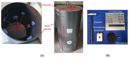
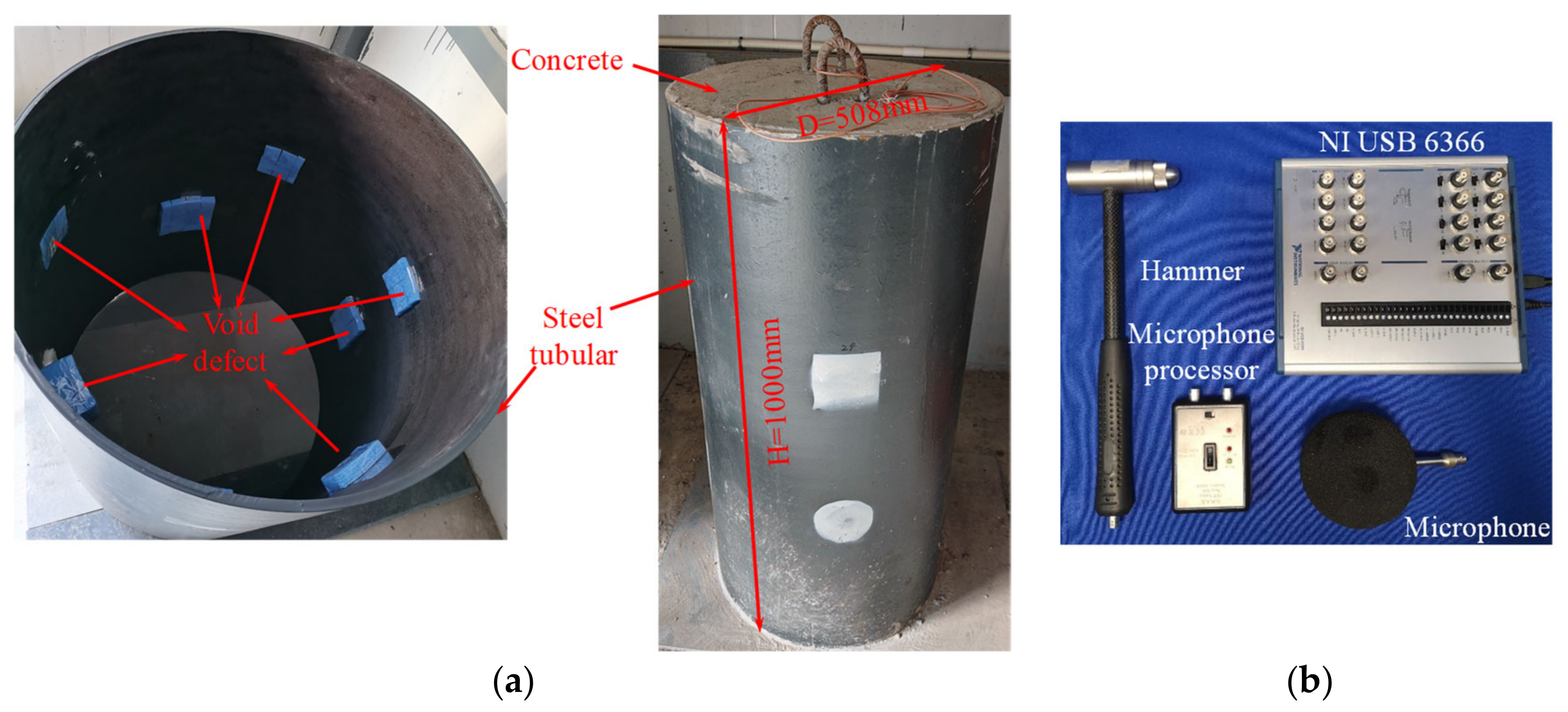
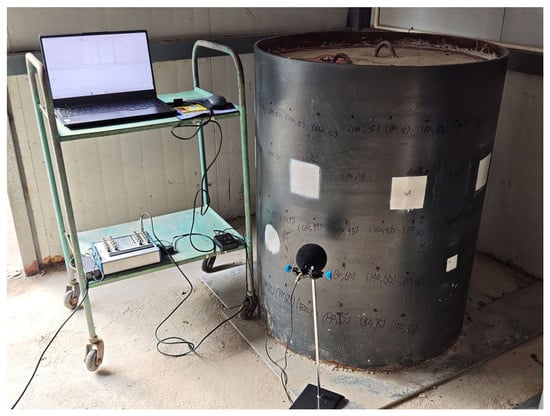
To verify the accuracy of the numerical acoustic-structure coupling model under the intact condition, percussion tests were conducted at an intact region of a CFST specimen containing pre-embedded simulated voids. The experimental setup is shown in Figure 1. The signals collected from the intact region were used only to compare the numerical and experimental acoustic responses under the non-debonded condition.

Figure 1. (a) CFST structure; (b) test equipment.

The CFST column featured an outer diameter of 508 mm, a wall thickness of 8 mm and a height of 1000 mm. The CFST specimen was fabricated using a Q355 steel tube and filled with grade C40 concrete. Plastic foam blocks were pre-embedded in designated regions of the concrete core to simulate voids of different sizes. Thus, the specimen contained both intact and simulated-void regions. For the numerical model validation presented in this section, the impact and microphone measurement positions were located in the intact region. A G.R.A.S 40PP CCP free-field quality control microphone (GRAS Sound & Vibration A/S, Holte, Denmark; serial number 238064) was employed to record the sound waves generated by hammer impacts. The captured signal was then amplified by a microphone processor and recorded on a laptop computer using an NI USB-6366 data acquisition device (National Instruments Corporation, Austin, TX, USA) equipped with a window denoising filter. To minimize errors, the percussion was conducted in a quiet and enclosed space. The microphone was positioned at a height of 250 mm above the ground, with a vertical distance of 40 mm from the surface of the steel tube. A sampling frequency of 100 kHz was adopted for the acquisition of impact-acoustic signals in the CFST percussion test to ensure the integrity of high-frequency signal features.

In this study, a multi-physics field coupling model of the CFST specimen was constructed by coupling the acoustic and structural fields to investigate the acoustic response of the CFST structure under transient conditions. The accuracy of the acoustic-structure coupling model for the intact condition was validated by comparing the simulated impact-acoustic signals with the signals measured at the intact region of the CFST specimen.

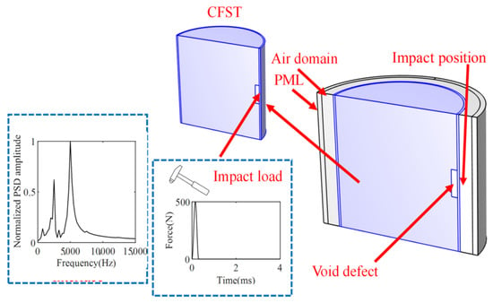
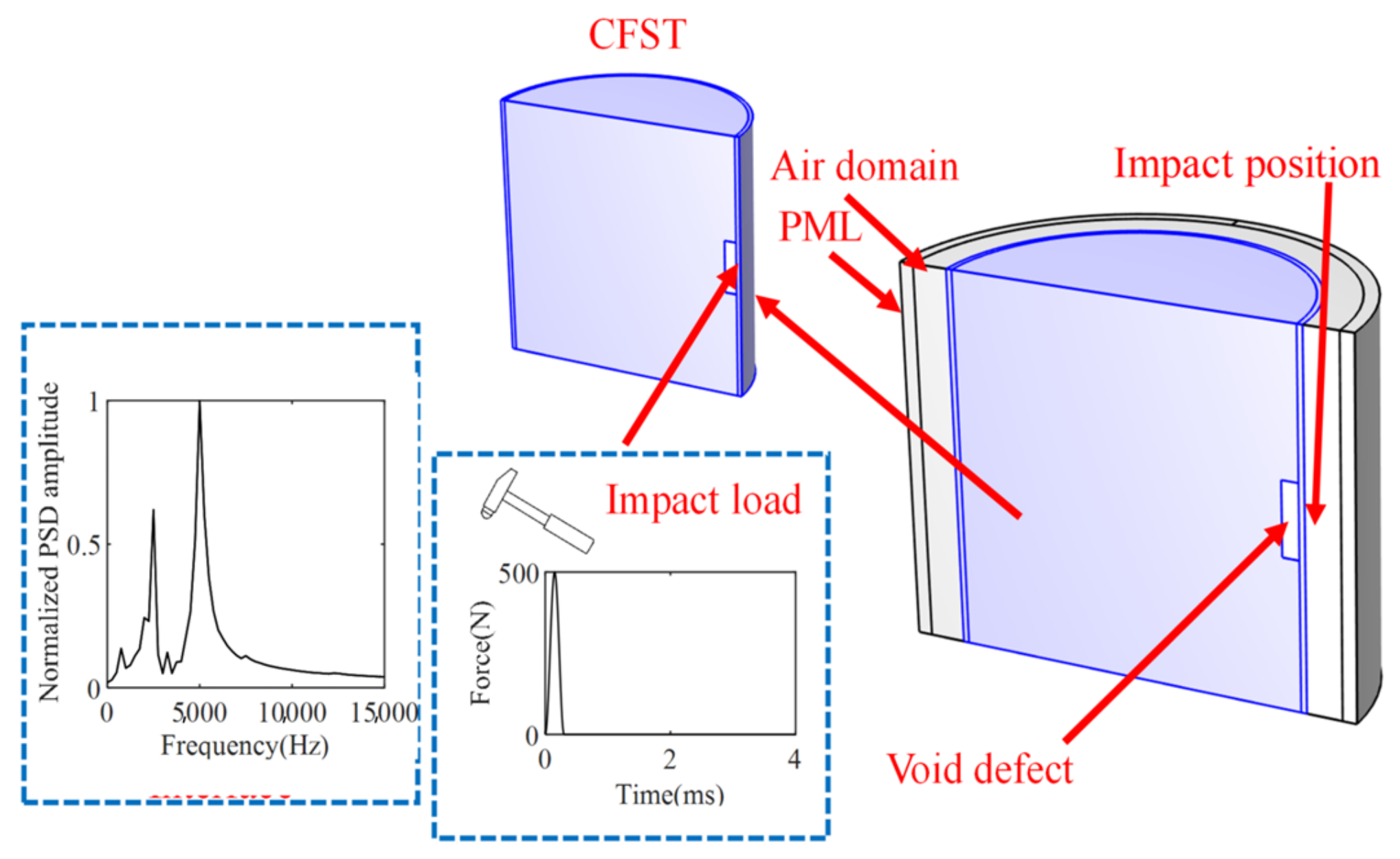
As depicted in Figure 2, the steel tube features an outer diameter of 508 mm, a wall thickness of 8 mm, and a height of 500 mm. The debonding defects are positioned at the mid-height of the steel tube. Additionally, the air domain is configured with the same height as the CFST structure, with its radial thickness set to 70 mm. The steel tube, concrete core, and air are meshed with 8-node elements, forming the finite element model (FEM) of the CFST structure. Acoustic-structure coupling boundary conditions are applied at the interface between the integral CFST structure and the surrounding air domain. The model incorporates a symmetry assumption to optimize computational efficiency and reduce memory consumption, and the corresponding symmetric boundary conditions are implemented accordingly. A Perfectly Matched Layer (PML) is applied at the outer boundary of the air domain as a non-reflective radiation boundary condition to simulate acoustic wave propagation in an infinite domain. Considering previous research, the PML thickness should be 1/4 to 1/2 of the dominant acoustic wavelength. In this study, the shortest wavelength is about 49 mm, corresponding to a maximum analysis frequency of 7 kHz. Therefore, the PML thickness was set to 20 mm, which is approximately 40% of the shortest acoustic wavelength. The PML’s density is set to 1.2 kg/m³, matching the adjacent air domain’s properties to ensure acoustic impedance continuity and minimize non-physical reflections at interfaces. The material properties are as follows: for the steel tube, the density is 7850 kg/m³, the modulus of elasticity is 200 GPa, and the Poisson’s ratio is 0.3. For the concrete, the density is 2400 kg/m³, the modulus of elasticity is 24 GPa, and the Poisson’s ratio is 0.167. The Rayleigh damping coefficient is 0.05. The mesh convergence study and parameter sensitivity analysis were not conducted. Therefore, the maximum element size of the acoustic–structure coupling model is set to 9.8 mm following the criterion of five elements per wavelength.

Figure 2. Acoustic-solid coupling FEM of CFST member.

To simulate the effect of an impact force, eliminate symmetric effects, and excite a variety of vibration modes, a sinusoidal pulse was applied at the central position on the outer surface of the CFST member to mimic a low-amplitude impact force. The load expression is given as follows:

$$F\left(t\right)=\{\begin{array}{cc}{F}_{\max }{\sin }^2\left({\displaystyle \frac{\pi }{T}}t\right)& 0\le t\le T\\ 0& t\ge T\end{array}$$

(1)

F(t) represents the impulse load, F_max denotes the peak impulse load (set to 500 N), and T signifies the load action time (set to 0.3 ms). The solution time step is set to 0.001 ms, the output time step to 0.01 ms, and the total simulation duration is 4 ms.

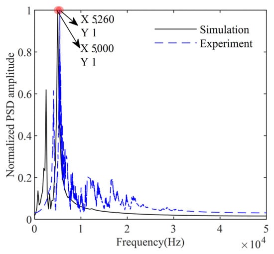
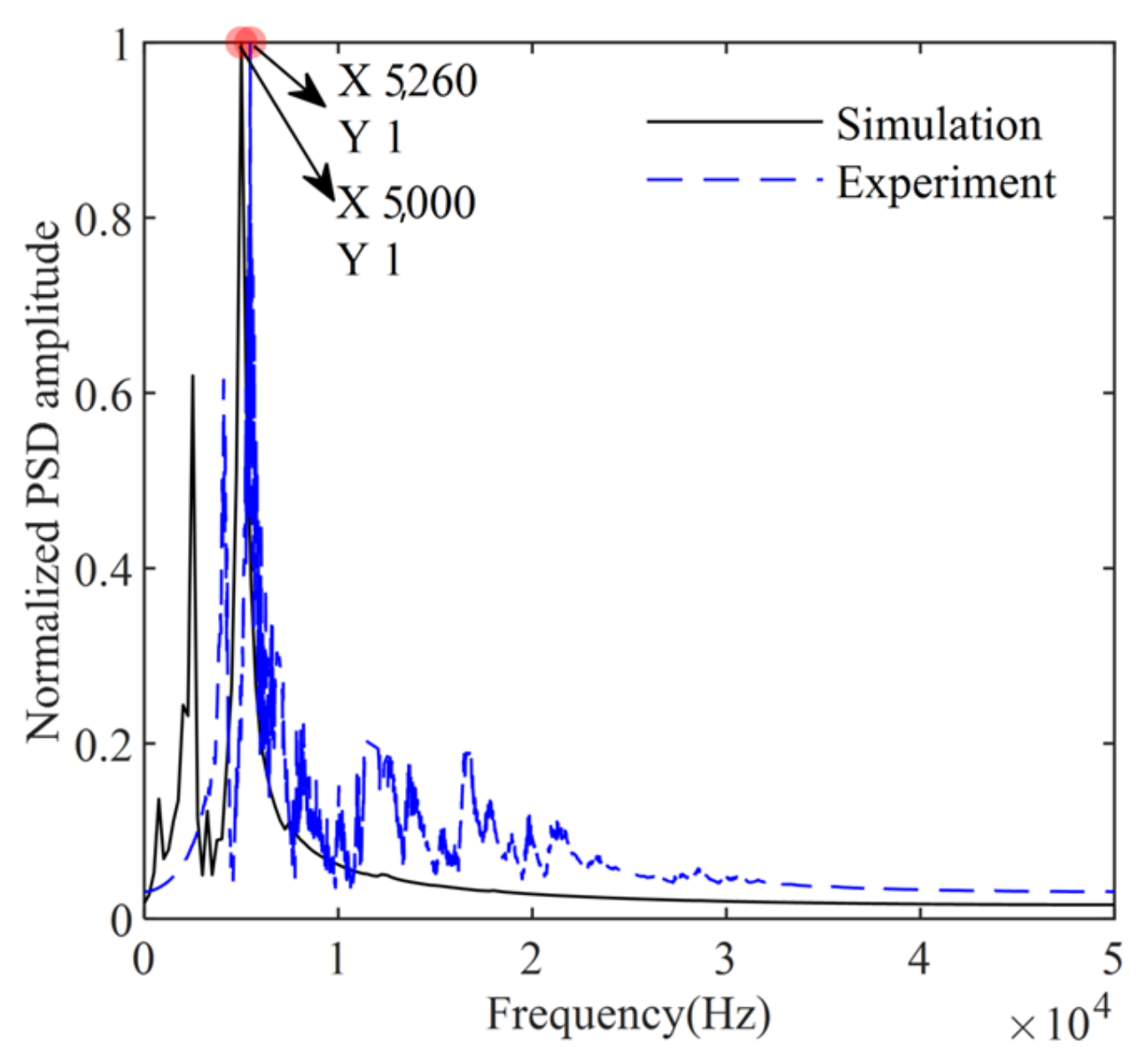
Figure 3 shows the power spectral density (PSD) of acoustic signals obtained from the numerical simulation and percussion tests conducted at the intact region of the CFST specimen. To facilitate the comparison of frequency response characteristics, the time-domain signals were normalized to minimize the influence of impact force on signal amplitude. The peak frequencies from the numerical simulation and experimental test are 5000 Hz and 5260 Hz, respectively, with a relative difference of 4.9%. The primary source of this error is the difference in impact forces. In the numerical simulations, a prescribed sine-squared pulse with a peak force of 500 N and a duration of 0.3 ms was applied to the CFST member, whereas the force-time history of a manual hammer impact may vary between experimental measurements. Additionally, minor discrepancies stem from slight differences between the microphone positions in the percussion tests and the points where sound pressure was extracted in the finite element analysis. Overall, background noise also has a certain influence.

Figure 3. Power spectrum densities without debonding defects.

2.2. Analysis on the Influence of Defects on Impact Signals

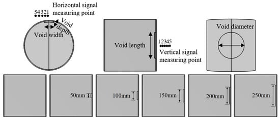
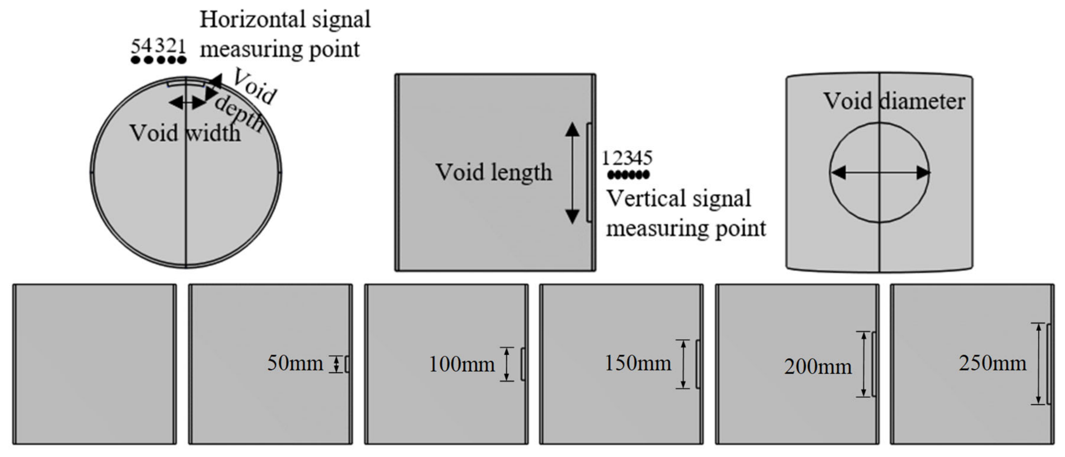
To further investigate the effects of defects on the characteristics of percussion signals, several scenarios were developed using numerical simulation techniques. Figure 4 illustrates the cross-sectional views of CFST structures with void lengths ranging from 0 to 250 mm. The simplified debonding defect configurations include:

Figure 4. Void working condition indication.

(1)

The intact condition;

(2)

A rectangular cross-section with a debonding length of 100 mm, debonding width of 100 mm, where the debonding depth is parameterized as 3, 6, 12, 24, and 72 mm;

(3)

A rectangular cross-section with a debonding width of 100 mm and a debonding depth of 12 mm, where the debonding length is parameterized as 50, 100, 150, 200, and 250 mm;

(4)

A rectangular cross-section with a debonding length of 100 mm and a debonding depth of 12 mm, where the debonding width is parameterized as 50, 100, 150, 200, and 250 mm;

(5)

A circular cross-section with a debonding depth of 12 mm and the diameter parameterized as 50, 100, 150, 200, and 250 mm;

(6)

A rectangular cross-section with a debonding depth of 12 mm and both debonding length and width of 100 mm. Acoustic signals are collected from five measurement points located at vertical distances of 10, 20, 30, 40, and 45 mm from the impact point, positioned at a horizontal distance of 0 mm along the steel tube with a height of 250 mm;

(7)

A rectangular cross-section with a debonding depth of 12 mm and both debonding length and width of 100 mm. Acoustic signals are collected from five measurement points located at horizontal distances of 0, 25, 50, 75, and 100 mm along the steel pipe, at a height of 250 mm and a vertical distance of 40 mm from the impact point.

The rectangular and circular void configurations adopted in the numerical simulations represent idealized local separations at the steel–concrete interface. The void length, width, or diameter characterizes the in-plane extent of the debonded region, whereas the void depth represents the separation gap between the steel tube and concrete. Although actual debonding defects may exhibit irregular boundaries and non-uniform interfacial gaps, the simplified geometries were adopted to isolate the effects of individual geometric parameters on the impact-acoustic response. The experimental tests described in Section 5 further evaluate the proposed method using CFST specimens with voids simulated by EPE foam blocks.

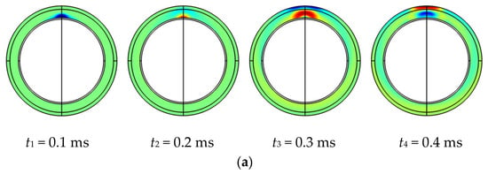
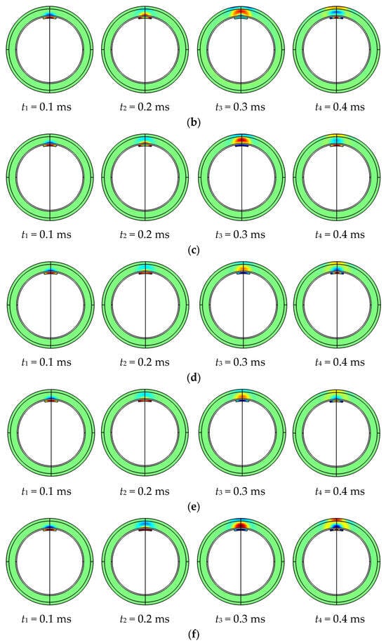
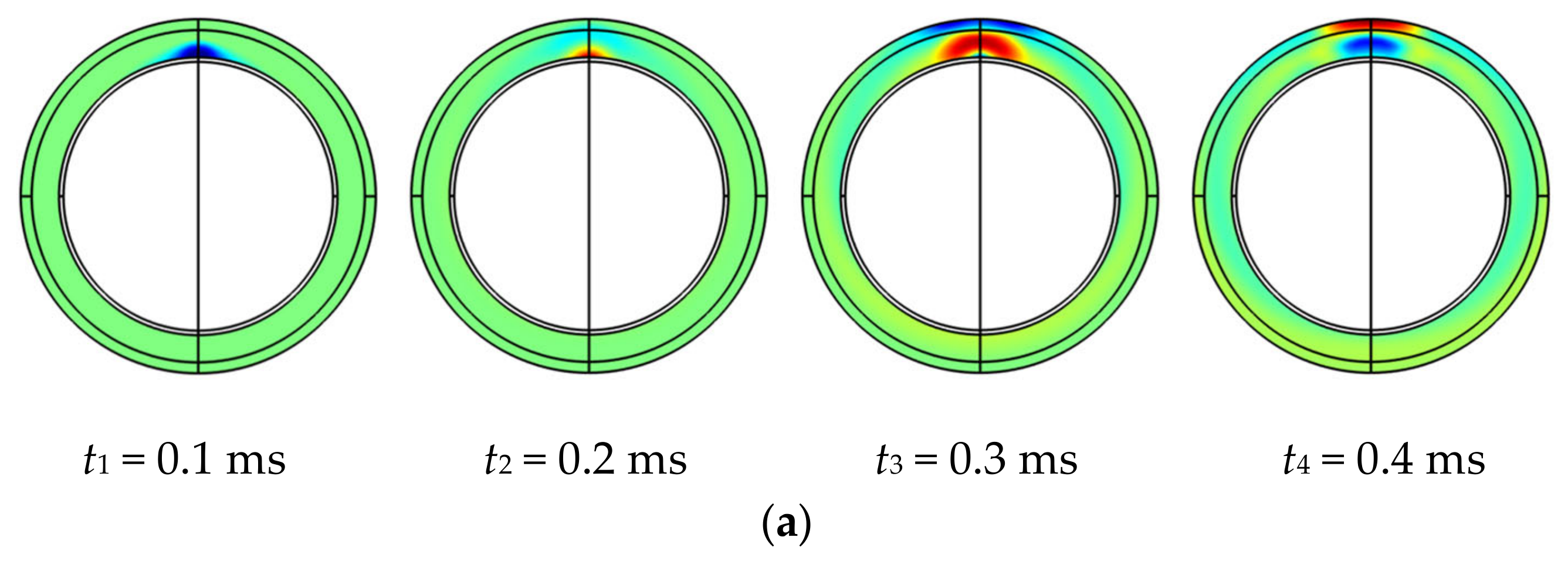
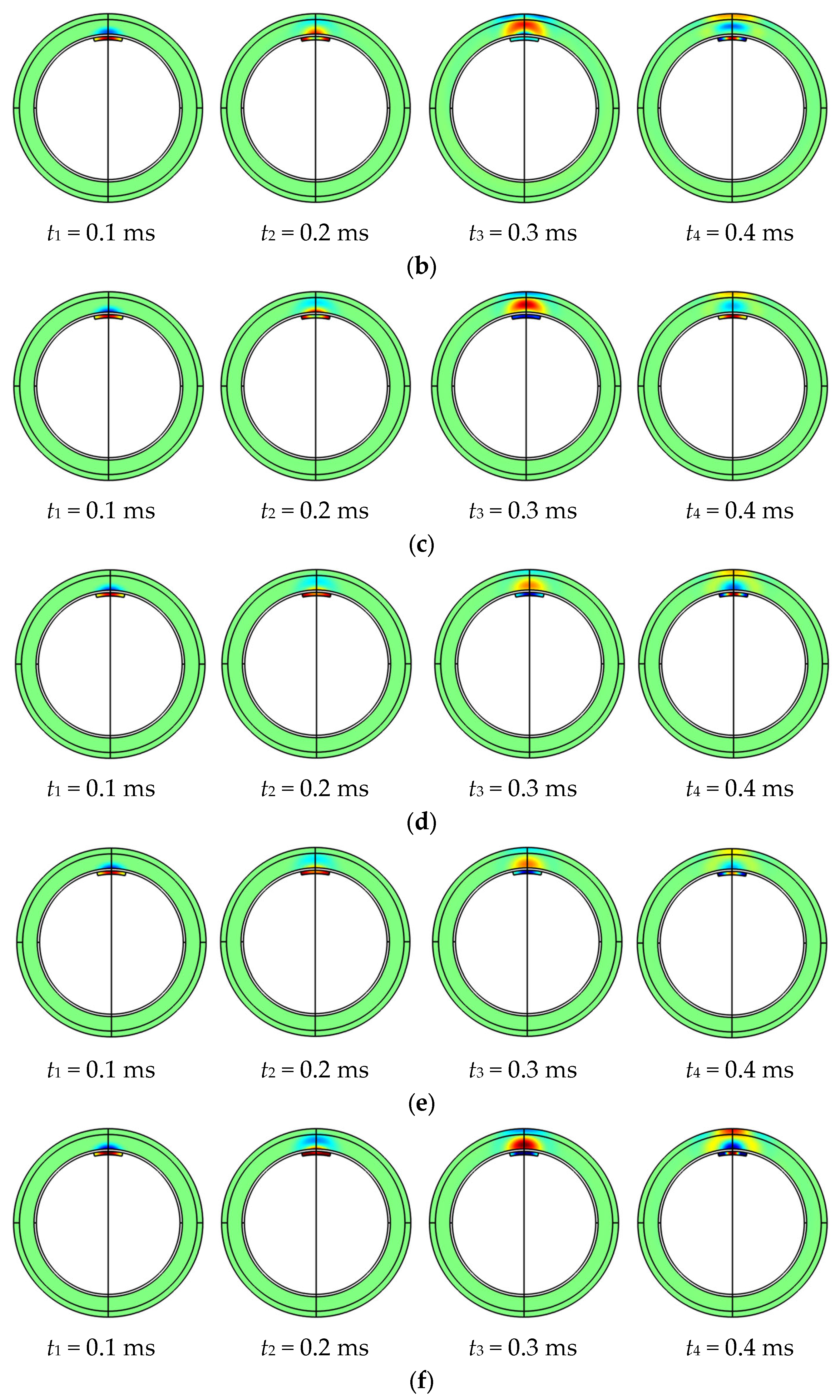
Acoustic pressure cloud maps at time intervals of t₁ = 0.1 ms, t₂ = 0.2 ms, t₃ = 0.3 ms and t₄ = 0.4 ms were analyzed, as shown in Figure 5. The distribution of acoustic pressure under different conditions shows noticeable variations, indicating that variations in void length affect acoustic wave propagation. This provides the potential for identifying and qualitatively analyzing debonding defects through acoustic signals.

Figure 5. Acoustic pressure distribution of different void lengths: (a) void length 0 mm; (b) void length 50 mm; (c) void length 100 mm; (d) void length 150 mm; (e) void length 200 mm; (f) void length 250 mm.

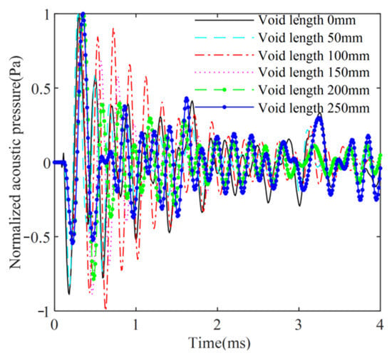
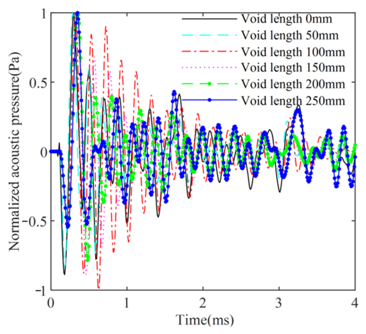
The normalized sound pressure analysis at a point with a height of 250 mm and a vertical distance of 40 mm from the structure surface is presented in Figure 6. The time-domain waveform of the percussion acoustic signal changed with different void lengths in the CFST structures. The presence of a debonding defect led to a gradual increase in the time-domain response period of the percussion acoustic signal, a slower decay rate and decay amplitude of the sound pressure, and an extended duration.

Figure 6. Acoustic pressure curves of different void lengths.

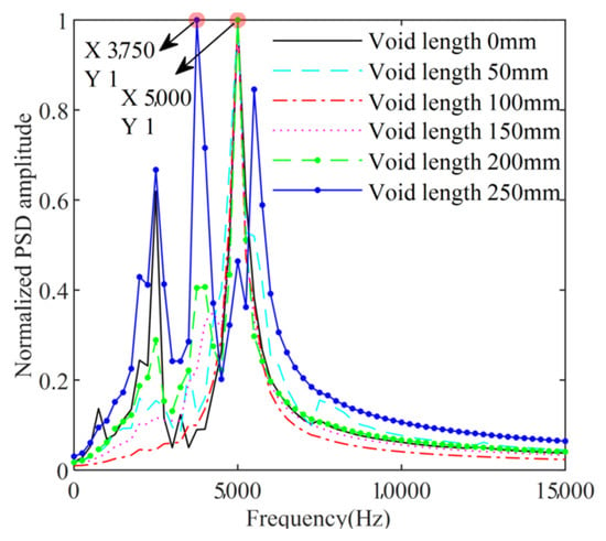
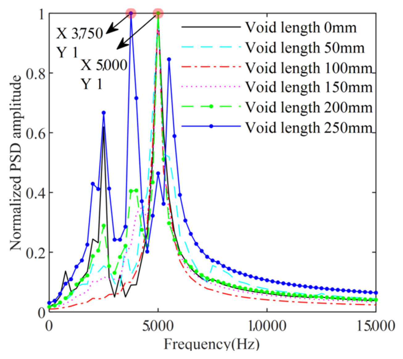
To assess the effects of varying debonding defect lengths on the frequency domain of the acoustic signal, the power spectrum of the acquired acoustic signal was estimated, and the resulting power spectral density (PSD) was normalized (Figure 7). The frequency of the acoustic signal was primarily distributed in the range of 0–7 kHz, and the shape of the PSD curve varied for different debonding lengths. The simulation results indicate that debonding defects have a noticeable influence on the acoustic signals, leading to changes in the attenuation rate of the time-domain waveform, the number of peak points in the power spectrum, and the peak frequency. Based on these findings, preliminary assessments were conducted to determine the presence of debonding defects.

Figure 7. Power spectrum densities of different void lengths.

3. Wavelet Packet Domain Feature Indicators Extraction

The core of this method lies in capturing acoustic wave characteristic variations caused by debonding: air cavity reflection decelerates energy attenuation, while localized resonance excitation alters the spectral profile. Simulation results from the previous section validate this physical mechanism, demonstrating that it fundamentally triggers a systematic redistribution of signal band energy. To quantify this critical physical phenomenon, this study employs wavelet packet analysis to extract the “band energy ratio” feature. Leveraging the inherent clustering tendency of this feature in the data space, unsupervised learning methods are utilized to automate damage diagnosis.

3.1. Wavelet Packet Energy Feature Extraction

Feature extraction involves using raw signals as the source signal to determine various parameters and form a feature vector that characterizes the signal’s features [41]. Wavelet packet analysis can effectively handle both the low-frequency and high-frequency components of a signal, allowing for a finer division of the frequency spectrum window. Compared to wavelet analysis, it offers superior time-frequency resolution and stronger signal processing capabilities, making it particularly suitable for extracting features from signals containing defect information [42]. In this study, wavelet packet analysis was utilized to analyze the percussion signals of CFST structures, selecting energy ratio values from different frequency bands to construct feature vectors for debonding defects.

The wavelet packet decomposition of the acoustic signal of the CFST structure y is performed at the i level, and the acoustic signal energy in each frequency band is calculated as follows:

$$E_{i,j}=\sum {\left|y_{i,j}\right|}^2\hspace{1em}(j=0,1,2,\cdots ,2^i-1)$$

(2)

y_i,j is the acoustic signal at the i layer node (i,j).

The wavelet packet energy E_i at the i layer is

E_i = {E_i,j} (j = 0,1,2,⋯,2ⁱ − 1)

(3)

The ratio of the energy of each band to the mean of the band energy is defined as the wavelet packet band energy ratio I_k is

$$I_k={\displaystyle \frac{E_{i,k}}{\raisebox{1ex}{$\sum _{j=0}^{2^i-1}{E}_{i,j}$}\!\left/ \!\raisebox{-1ex}{$2^i$}\right.}}\hspace{1em}\left(k=0,1,2,\cdots ,\mathrm{m}\right)$$

(4)

Determining structural debonding by changes in I_k

ERV_k = |I_uk − I_dk| (k = 0,1,2,⋯,m)

(5)

ERV_k is the change in energy ratio in the k band; I_uk and I_dk are the energy ratios in the k band for CFST structures without and with debonding respectively.

Three indices for the identification of debonding defects in CFST structures are defined based on the wavelet packet band energy ratio variation ERV_k.

(1)

Cumulative energy-ratio difference index DI

$$\mathrm{DI}={\displaystyle \sum _{k=0}^m}{\displaystyle \frac{{\mathrm{ERV}}_k}{I_{\mathit{uk}}}}$$

(6)

The DI represents the cumulative relative change in wavelet packet energy distribution caused by debonding. A larger DI indicates a more significant overall deviation of the debonded signal from the intact signal.

(2)

Energy ratio deviation ERVD

$$\mathrm{ERVD}=\sqrt{{\displaystyle \sum _{k=0}^m}{\left({\mathrm{ERV}}_k-\overline{\mathrm{ERV}}\right)}^2}$$

(7)

where $\overline{\mathrm{ERV}}$ is the mean value of ERV_k over the selected frequency bands. ERVD describes the dispersion degree of the energy-ratio variation among different frequency bands. A larger ERVD indicates that debonding causes more uneven redistribution of signal energy across the frequency bands.

(3)

Energy Ratio Variance ERVV

$$\mathrm{ERVV}={\displaystyle \frac{\sum _{k=0}^m{\left({\mathrm{ERV}}_k-\overline{\mathrm{ERV}}\right)}^2}{m}}$$

(8)

$\overline{\mathrm{ERV}}$ is the average of the energy ratio changes in each band ERV_k. ERVV quantifies the variance of the defect-induced energy redistribution. Compared with DI, ERVD and ERVV are more sensitive to non-uniform changes in frequency-band energy distribution, which are usually associated with more pronounced debonding defects.

3.2. Determining Parameters for Wavelet Packet Transform

(1)

Selection of wavelet function

A seven-level wavelet packet decomposition using Daubechies wavelets db4–db13 was performed on the percussion signal of an intact CFST structure, and the corresponding cost function values were calculated using Equation (9). As shown in Table 1, db9 yielded the lowest cost function value among the wavelets examined and was therefore adopted for subsequent analyses. This selection was based on the cost function evaluated for the intact signal, rather than on a direct comparison of defect-identification performance.

$$S_L\left({\mathit{E}}_i\right)=\sum _j{\left|E_{i,j}\right|}^p\hspace{1em}\left(j=0,1,2,\cdots ,2^i-1\right)$$

(9)

Table 1. Cost function values for different dbN.

Wavelet Level N	SL(Ei) (p = 1.5)
4	29.3
5	33.4
6	43.4
7	27.9
8	34.8
9	24.7
10	44.1
11	46.1
12	65.0
13	51.2

(2)

Selection of wavelet packet decomposition levels

Wavelet packet decomposition using db9 was performed at levels 3–7 on the percussion signal of an intact CFST structure. As shown in Table 2, the seven-level decomposition yielded the lowest cost function value among the tested levels. Although it required the longest computational time, the processing duration of 0.3079 s was considered acceptable for the present analysis. Accordingly, seven levels were adopted for subsequent analyses. However, the minimum cost function value does not establish that this decomposition level provides the best defect-classification performance.

Table 2. Cost function values and computing time for different decomposition levels.

Level i	3	4	5	6	7
SL(Ei)(p = 1.5)	129.2	94.8	67.2	48.5	24.7
Time (s)	0.1666	0.1731	0.2034	0.2440	0.3079

The db9 wavelet and seven-level decomposition are therefore treated as the adopted processing settings in this study. No comparative identification analysis was conducted across alternative wavelet bases and decomposition levels. Consequently, their optimality for defect classification has not been established. The clustering comparisons reported in Section 4 evaluate different clustering methods using the adopted feature-extraction settings and do not constitute a comparison of wavelet parameter choices.

(3)

Selection of wavelet packet frequency bands

The correlation coefficients between the original signal and the reconstructed signals from the first 10, 13, 16, and 20 wavelet packet bands were calculated as 0.5985, 0.9174, 0.9718, and 0.9732, respectively. The correlation analysis was used to evaluate the reconstruction fidelity of the selected frequency bands. When the first 20 bands were included, the cumulative reconstructed signal showed a high correlation with the original signal. The DI, ERVD, and ERVV indicators calculated from these bands further exhibited systematic variations with the simulated void geometries, as presented in Section 3.3. Accordingly, the first 20 frequency bands were retained for subsequent feature extraction. This selection ensured adequate signal reconstruction fidelity while preserving energy-distribution differences relevant to debonding identification.

3.3. Analysis of Debonding Characteristic Indicators

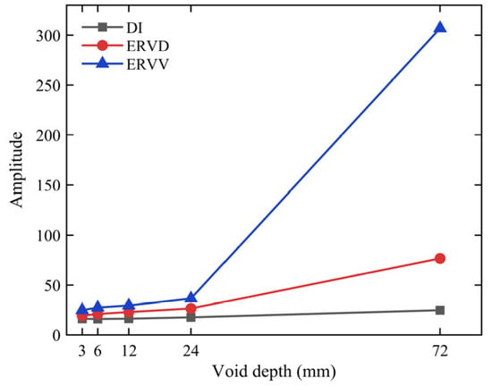
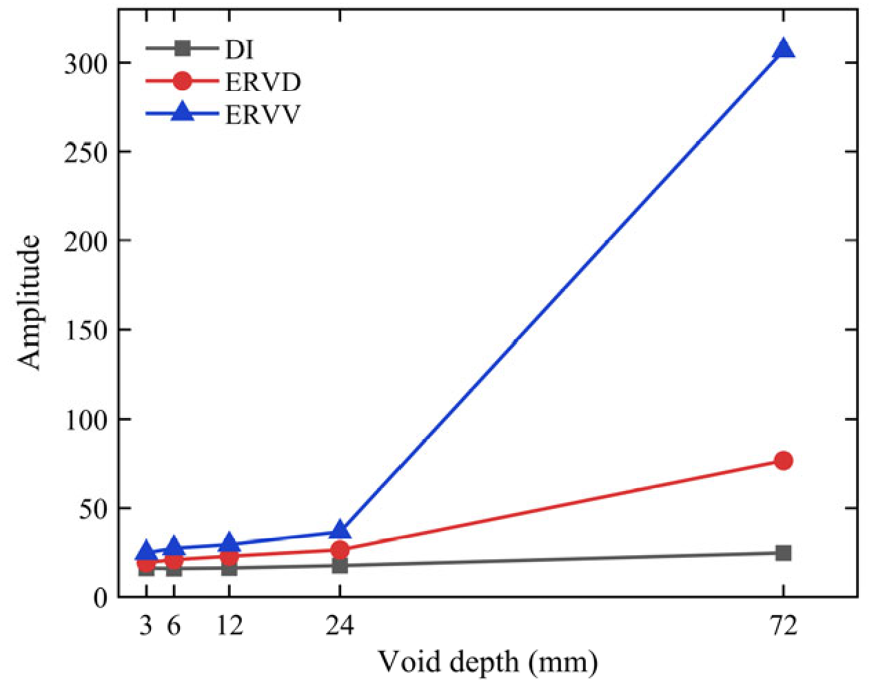
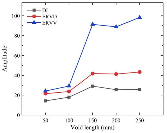
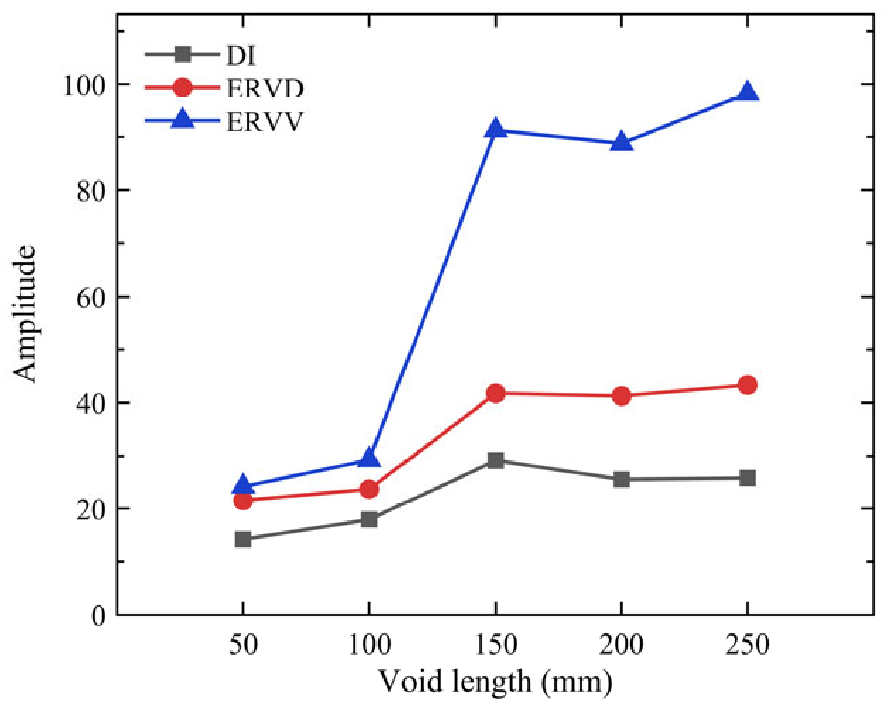
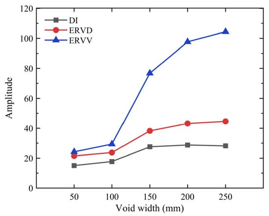
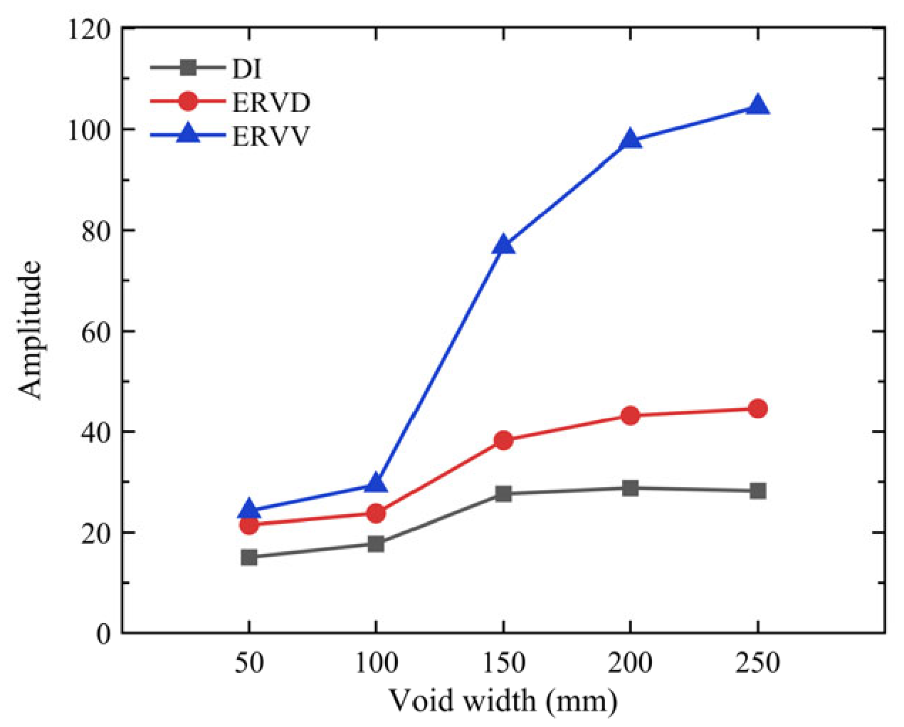
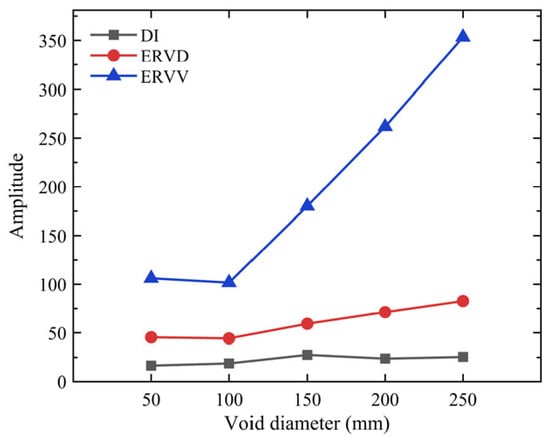
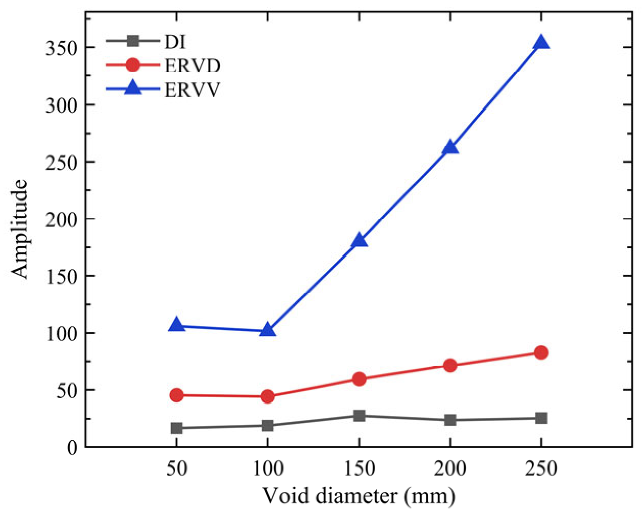
The cumulative energy-ratio difference index, energy ratio deviation, and energy ratio variance for CFST structures under different operational conditions are derived from Equations (6)–(8) and presented in Figure 8, Figure 9, Figure 10 and Figure 11.

Figure 8. Indicator amplitude of different void depths.

Figure 9. Indicator amplitude of different void lengths.

Figure 10. Indicator amplitude of different void widths.

Figure 11. Indicator amplitude of different void diameters.

As depicted in Figure 8, Figure 9, Figure 10 and Figure 11, with the increase in the depth, length, and width of rectangular voids, as well as the diameter of circular voids, although there are occasional decreases at individual points, overall, there is an increasing trend in the three indicators. Significant differences in parameter values are evident among different debonding defect states, and the reasonable selection of empirical thresholds enables the determination of debonding defects in CFST structures. While distinct numerical outcomes are obtained for various void types using the same indicators, the underlying trends of these indicators remain largely consistent.

When comparing the three indicators, it becomes apparent that the DI indicator is less sensitive to changes in debonding defects than the ERVD and ERVV indicators, making it suitable for applications where the degree of debonding is minimal. As the void size increases, the ERVD and ERVV exhibit greater sensitivity to defects than the DI. Moreover, the rate of increase in ERVV is significantly higher than that of ERVD. Within the simulated void configurations considered, ERVV exhibited a greater increase with increasing void size than ERVD. These observations are restricted to the simulated void geometries considered in the numerical analysis. They do not establish indicator-selection rules for different stages of in-service debonding or demonstrate performance for naturally occurring defects.

4. Experimental Specimen and Impact Testing

4.1. Experimental Specimen and Impact Signal Acquisition

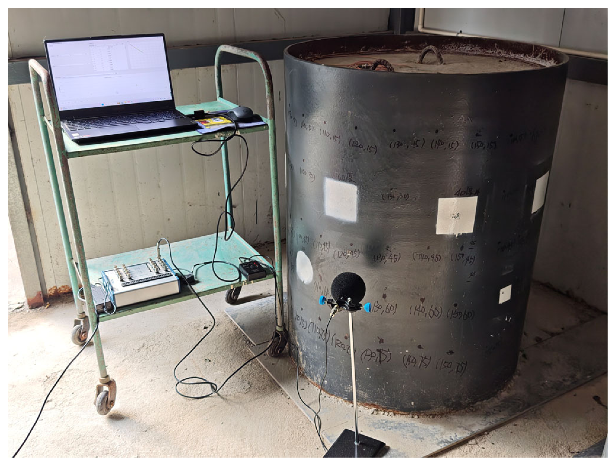
To validate the capability of the proposed method to identify void defects in a physical specimen, a circular CFST specimen with an outer diameter of 800 mm and a wall thickness of 10 mm was tested. The steel tube was fabricated from Q235 steel and filled with C30 concrete. Expanded polyethylene (EPE) foam blocks were affixed to the inner surface of the steel tube in designated regions to simulate void defects. Multiple impact locations were arranged on the specimen surface in both void and non-void regions. Five baseline impact locations were established in the non-void region, whereas the remaining locations were arranged within the void region according to the different experimental conditions. The experimental setup is shown in Figure 12. The experimental investigation was conducted on a single CFST specimen containing EPE-foam simulated voids. Repeated impacts and measurements at different locations characterize variability within this specimen and do not provide independent validation across specimens.

Figure 12. Experimental setup for impact signal acquisition.

The CFST specimen was excited by impact, and the resulting acoustic signals were recorded using a microphone. The microphone height was set to the elevation of the void center, and the microphone was positioned 50 mm normal to the steel tube surface. The sampling frequency was 20 kHz. To reduce the influence of random variations in individual impacts, five repeated impacts were performed at each impact location, and the signal from each impact was saved separately as a TXT file. The tests considered a quiet environment, background noise, denoising, variations in microphone position, and variations in impact position. The specific experimental conditions were as follows:

(1)

Intact condition without void defects.

(2)

Rectangular voids with a width of 100 mm, a length of 100 mm, and thicknesses of 5, 10, 20, and 40 mm, as well as a rectangular void with a width of 150 mm, a length of 150 mm, and a thickness of 20 mm. Acoustic signals were acquired under both quiet and background-noise conditions.

(3)

A rectangular void with a width of 100 mm, a length of 100 mm, and a thickness of 40 mm. The microphone center was positioned at a height of 650 mm above the ground. For vertical microphone-position variation, acoustic signals were acquired at three measurement locations with a horizontal distance of 0 mm and vertical distances of 40, 60, and 80 mm from the impact point. For horizontal microphone-position variation, acoustic signals were acquired at three measurement locations with a vertical distance of 50 mm and horizontal distances of 0, 50, and 100 mm from the impact point.

(4)

A rectangular void with a thickness of 40 mm, a length of 100 mm, and a width of 100 mm. With the microphone positioned at a height of 650 mm and 50 mm normal to the steel tube surface, acoustic signals were acquired at five impact locations with horizontal distances of 0, 25, 50, 75, and 100 mm from the void center.

4.2. Signal Preprocessing and Wavelet Packet Feature Extraction

To establish a consistent time reference for signals acquired under different experimental conditions and from repeated impacts, the recorded raw acoustic signals were first segmented. Based on the time-domain response of the impact signals, the sample with the maximum absolute amplitude was defined as the impact reference point. Signal segments extending 0.03 s before and 0.20 s after this reference point were retained. The 0.03 s pre-peak interval preserved the short-duration background and signal-rising process before the impact peak, while reducing the effects of variations in reference-point localization and signal truncation. The 0.20 s post-peak interval covered the principal vibration and decay processes of the impact response while limiting the inclusion of irrelevant background noise associated with an excessively long time window. At a sampling frequency of 20 kHz, each segmented signal contained 4601 samples, with the impact reference point located at the 601st sample. This procedure ensured consistent signal length and feature dimensionality across different experimental conditions. Signals for which the extraction window extended beyond the boundaries of the raw record or whose peak positions were clearly abnormal were not directly included in the subsequent feature extraction and clustering analyses.

For raw signals substantially longer than 4601 samples, uniform segmentation was performed automatically according to the sample with the maximum absolute amplitude. Signals that had already been segmented and whose peak positions fell within the allowable tolerance were used directly for subsequent processing. If a signal had a length close to 4601 samples but an obviously abnormal peak position, it was examined individually and was not directly included in the feature extraction and clustering analyses. After uniform segmentation, DC offsets were removed from all signals, after which peak normalization was performed. These operations reduced the effects of DC bias and variations in impact force on the overall signal amplitude.

The experimental signals were processed using the wavelet packet feature-extraction method described in Section 3. Because the experimental tests and numerical simulations differed in sampling frequency, analysis window, and signal-frequency distribution, the number of retained frequency bands was redetermined for the experimental signals. Signals acquired from the non-void region under quiet conditions were used as reference signals. A seven-level wavelet packet decomposition was performed using the Daubechies 9 (db9) wavelet, yielding 128 terminal frequency bands. The db9 wavelet and seven-level decomposition were retained as the processing settings adopted in Section 3.2; they were not selected through a separate comparison of classification performance on the experimental dataset. The terminal nodes were ordered from low to high frequency, and the reconstructed signals of the individual bands were then accumulated sequentially. Following the procedure described in Section 3.2, Pearson correlation coefficients were calculated between the cumulative reconstructed signals and the original preprocessed signals. When the first 92 terminal frequency bands were retained, the correlation coefficient between the cumulative reconstructed signal and the original signal reached approximately 0.95. Therefore, the energy ratios of the first 92 frequency bands were selected as the wavelet packet features of the experimental signals.

After determining the number of retained frequency bands, the wavelet basis function, decomposition level, band-ordering method, and number of retained bands were kept unchanged for all experimental conditions. The energy and energy ratio of each of the first 92 frequency bands were calculated according to the procedures given in Section 3.1, thereby representing each impact-acoustic signal as a 92-dimensional wavelet packet energy-ratio feature vector. This feature-extraction procedure was applied consistently to all experimental conditions, including non-void samples, different void sizes, variations in microphone position, variations in impact position, background noise, and denoising, thereby ensuring consistent and comparable feature definitions across samples.

The 92-dimensional feature vectors of all samples were arranged row-wise to form the feature matrix for unsupervised clustering. Before clustering, each feature dimension was standardized using Z-score normalization to reduce the effects of differences in feature scale among frequency bands on inter-sample distance calculations and clustering results. The standardized feature matrix was used as the common input for subsequent clustering analyses.

4.3. Clustering Methods and Evaluation Metrics

The standardized 92-dimensional wavelet packet energy-ratio feature matrix obtained in Section 4.2 was used as the input for clustering. Unlike the single linkage criterion used for the numerical simulations in Section 4, agglomerative hierarchical clustering (AHC) for the experimental data employed the Ward linkage criterion. Single linkage defines the distance between two clusters according to the closest pair of samples from the two clusters and is therefore susceptible to bridging samples and the chaining effect [43]. By contrast, the Ward linkage criterion minimizes the increase in within-cluster dispersion caused by cluster merging and tends to produce relatively compact clusters [44]. Because manual impacts, variations in measurement locations, and background noise may induce fluctuations in sample features, Euclidean distance was used to calculate inter-sample distances, and the Ward linkage criterion was used for cluster merging in the experimental clustering analysis. The number of clusters was set to two.

To compare the suitability of different clustering mechanisms for the experimental signal features, K-means, K-medoids, NMF-based clustering, PCA-GMM, spectral clustering, and PCA-DBSCAN were further selected as comparison methods. K-means and K-medoids are partitioning-based clustering methods [45,46]; NMF-based clustering is a matrix-factorization-based clustering method [47]; PCA-GMM is a probabilistic-model-based clustering method [48]; spectral clustering is a graph-based clustering method [49]; and PCA-DBSCAN is a density-based clustering method [50].

Because high-dimensional, small-sample data may lead to an excessive number of Gaussian mixture model parameters and increase the risk of covariance-matrix singularity [51], PCA was applied to the standardized features before GMM clustering [52]. All principal components required to achieve a cumulative explained variance of 90% were retained, thereby preserving the main information while reducing the number of model parameters. The number of GMM clusters was set to two, corresponding to the void and non-void states. Unshared diagonal covariance matrices were adopted to reduce the number of covariance parameters while allowing the two clusters to have different covariance structures. The covariance regularization parameter was set to 1 × 10⁻⁵ to improve the numerical stability of model fitting. The maximum number of iterations was set to 1000 to prevent premature termination before sufficient convergence, and 20 replicate runs were performed to reduce the influence of random initialization. For DBSCAN, PCA were likewise applied before clustering; however, all principal components required to achieve a cumulative explained variance of 95% were retained to preserve the local neighborhood structure of the samples as much as possible while reducing the feature dimensionality. Neither PCA procedure used the true sample labels.

For K-means, the number of clusters was set to two, squared Euclidean distance was used to measure the difference between samples and cluster centroids, the maximum number of iterations was set to 1000, and 50 replicate runs were performed to reduce the effect of randomly initialized cluster centroids. K-medoids also used squared Euclidean distance and the partitioning around medoids (PAM) algorithm to select cluster centers from the observed samples, thereby reducing the influence of extreme samples on the cluster centers. The number of clusters was set to two, and 50 replicate runs were performed. For NMF-based clustering, the unstandardized 92-dimensional wavelet packet energy-ratio features were first normalized feature-wise to the interval [0, 1] to satisfy the input requirement of non-negative matrix factorization and reduce the effects of different feature ranges. The factorization rank was set to two, corresponding to the two sample states. The factorization was solved using the multiplicative-update algorithm, with a maximum of 1000 iterations. Both the function-value and variable convergence tolerances were set to 1 × 10⁻⁵ to obtain a sufficiently stable factorization while avoiding unnecessary iterations. Fifty replicate runs were performed to reduce the influence of random initialization. Sample labels were determined according to the component with the largest weight in the coefficient matrix.

For spectral clustering, Euclidean distances between the standardized features were first calculated and transformed into similarities using a Gaussian kernel. The kernel width was set to the median of all nonzero pairwise sample distances to reduce the effect of a small number of extreme distances on the similarity scale. The diagonal elements of the similarity matrix were set to zero to exclude self-connections. A symmetric normalized graph Laplacian matrix was then constructed to reduce the influence of differences in sample connectivity on spectral decomposition. The eigenvectors corresponding to the two smallest eigenvalues were selected to obtain a low-dimensional representation associated with the two potential clusters. After normalization, K-means was applied to partition the samples into two clusters, with a maximum of 1000 iterations and 50 replicate runs.

Given the small number of samples in the experimental dataset, MinPts for PCA-DBSCAN was set to three to avoid classifying an excessive number of samples as noise because of overly stringent density requirements. Because an excessively small ε produces many noise samples, whereas an excessively large ε may merge distinct clusters, the candidate range was determined from the third-nearest-neighbor distances corresponding to MinPts. A total of 120 candidate ε values were generated uniformly between the fifth percentile and the maximum of the third-nearest-neighbor distances, thereby balancing the search range, search resolution, and computational cost. Only results that formed two valid clusters with at least two samples in each cluster were retained, ensuring that the internal clustering metrics could be calculated meaningfully. The product of the mean Silhouette coefficient of the non-noise samples [53] and Coverage was used to select ε. This criterion considers both cluster separation and sample coverage and avoids obtaining favorable internal metrics by discarding a large number of samples. The parameter-selection procedure did not use the true sample labels.

The cluster labels produced by unsupervised clustering do not inherently correspond to the physical states of void and non-void samples. Therefore, cluster labels were mapped to physical classes after clustering. The true labels were defined as 0 for non-void samples and 1 for void samples. The two possible cluster-label mappings were compared, and the mapping that yielded the higher accuracy was adopted. The true labels were used only for post-clustering label mapping and performance evaluation; they were not used during signal preprocessing, feature extraction, PCA dimensionality reduction, or clustering.

To quantitatively evaluate the clustering results, accuracy, precision, recall, and confusion matrices were used to assess the agreement between the clustering results and the actual void states. The Silhouette coefficient and Davies–Bouldin index [54] were also used to evaluate the internal structure of the clustering results. Accuracy denotes the proportion of correctly identified samples among all samples. Precision denotes the proportion of true void samples among the samples identified as void. Recall denotes the proportion of actual void samples that were correctly identified. A larger Silhouette coefficient generally indicates greater within-cluster compactness and between-cluster separation, whereas a smaller Davies–Bouldin index generally indicates a more appropriate clustering structure.

Because DBSCAN allows samples located in locally low-density regions to be classified as noise, the number of noise samples, Coverage, and non-noise accuracy were additionally reported for PCA-DBSCAN. Non-noise accuracy was calculated only for samples assigned to valid clusters. Overall accuracy was calculated using all samples, with noise samples treated as incorrectly identified.

4.4. Experimental Results Analysis and Discussion

4.4.1. Clustering Results in a Quiet Environment

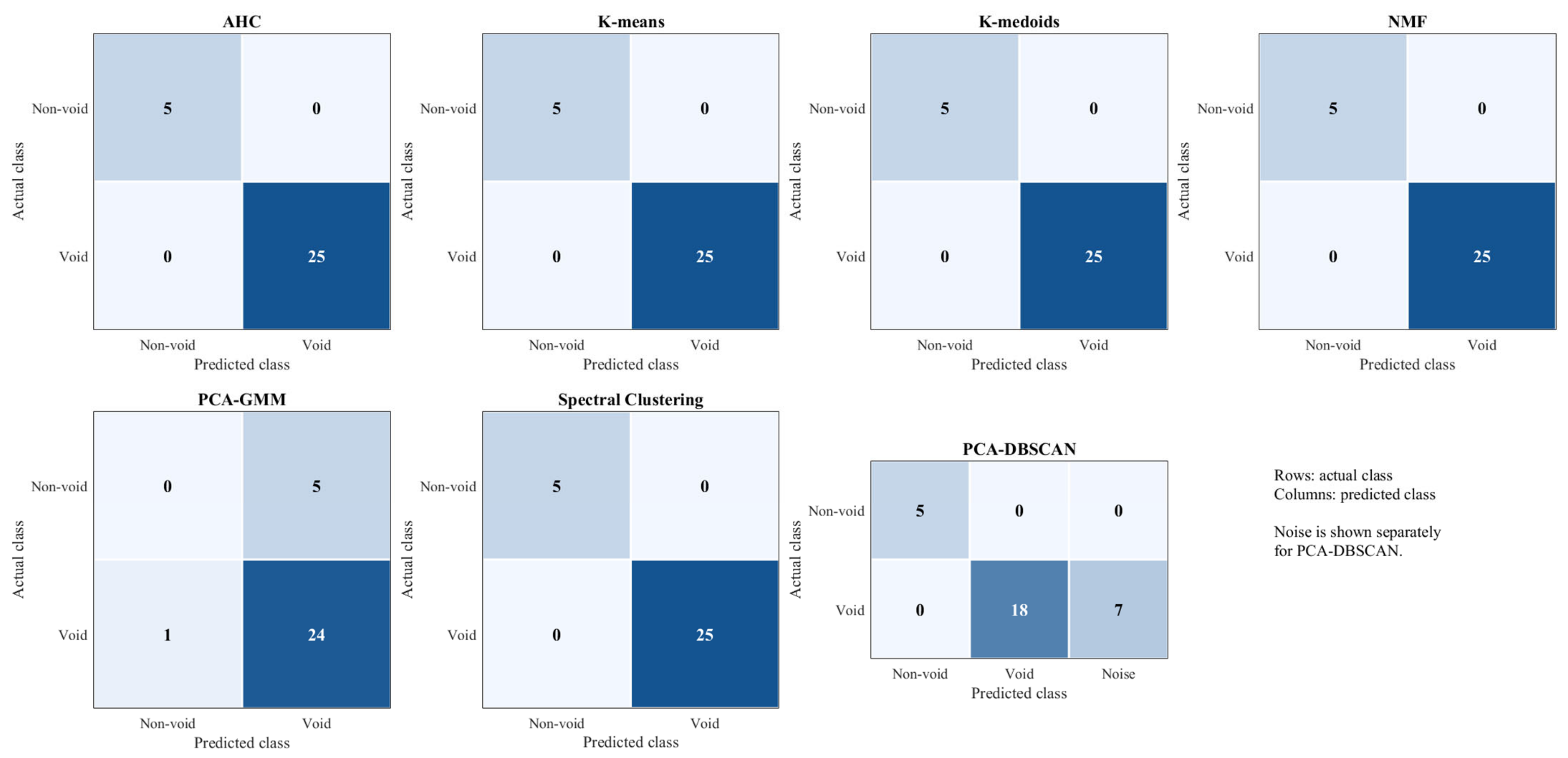
To evaluate the identification performance of the seven clustering methods under quiet conditions, Table 3 presents the quantitative evaluation metrics for each method, and Figure 13 further shows the confusion matrices for the void and non-void samples.

Table 3. Clustering results in a quiet environment.

Method	Accuracy (%)	Precision (%)	Recall (%)	Silhouette	Davies–Bouldin	Noise Samples	Coverage (%)	Non-Noise Accuracy (%)
AHC	100.00	100.00	100.00	0.1549	1.3216	-	-	-
K-means	100.00	100.00	100.00	0.1549	1.3216	-	-	-
K-medoids	100.00	100.00	100.00	0.1549	1.3216	-	-	-
NMF	100.00	100.00	100.00	0.1549	1.3216	-	-	-
PCA-GMM	80.00	82.76	96.00	N/A	N/A	-	-	-
Spectral	100.00	100.00	100.00	0.1549	1.3216	-	-	-
PCA-DBSCAN	76.67	100.00	72.00	0.2298	1.2053	7	76.67	100.00

Figure 13. Confusion matrices of the seven clustering methods in a quiet environment.

AHC, K-means, K-medoids, NMF, and spectral clustering correctly identified all samples, with Accuracy, Precision, and Recall all reaching 100.00%. These results indicate that the extracted 92-dimensional wavelet packet energy-ratio features can effectively distinguish void and non-void samples under quiet conditions.

By contrast, PCA-GMM achieved an Accuracy of 80.00%, a Precision of 82.76%, and a Recall of 96.00%. These results indicate that PCA-GMM identified most void samples but showed relatively poorer discrimination of non-void samples. Because the PCA-GMM clustering results contained a cluster with only one sample, the Silhouette coefficient and Davies–Bouldin index could not be meaningfully calculated and are therefore reported as N/A in the table.

PCA-DBSCAN achieved an overall Accuracy of 76.67% and classified seven samples as noise, resulting in a Coverage of 76.67%. For samples assigned to valid clusters, both Non-noise Accuracy and Precision were 100.00%, indicating that PCA-DBSCAN accurately separated the samples retained in the valid clusters. However, because some void samples were classified as noise, Recall decreased to 72.00%, which consequently reduced the overall Accuracy.

Overall, under quiet conditions, AHC, K-means, K-medoids, NMF, and spectral clustering showed good void-identification performance. In particular, AHC achieved correct classification of all samples without requiring prior dimensionality reduction or density parameters, demonstrating its feasibility for void identification using experimental impact-acoustic signals.

4.4.2. Influence of Background Noise and Denoising

To examine the effects of background noise and denoising on identification performance, Table 4 presents the results of the seven clustering methods under two signal conditions: with background noise and after denoising.

Table 4. Clustering results with background noise and after denoising.

Method	Signal Condition	Accuracy (%)	Precision (%)	Recall (%)	Silhouette	Davies- Bouldin	Noise Samples	Coverage (%)	Non-Noise Accuracy (%)
AHC	With Background Noise	100.00	100.00	100.00	0.1068	1.5440	-	-	-
	After Denoising	100.00	100.00	100.00	0.1675	1.4258	-	-	-
K-means	With Background Noise	100.00	100.00	100.00	0.1068	1.5440	-	-	-
	After Denoising	100.00	100.00	100.00	0.1675	1.4258	-	-	-
K-medoids	With Background Noise	96.67	100.00	96.00	0.1106	1.9983	-	-	-
	After Denoising	100.00	100.00	100.00	0.1675	1.4258	-	-	-
NMF	With Background Noise	100.00	100.00	100.00	0.1068	1.5440	-	-	-
	After Denoising	100.00	100.00	100.00	0.1675	1.4258	-	-	-
PCA-GMM	With Background Noise	80.00	82.76	96.00	N/A	N/A	-	-	-
	After Denoising	80.00	82.76	96.00	N/A	N/A	-	-	-
Spectral Clustering	With Background Noise	100.00	100.00	100.00	0.1068	1.5440	-	-	-
	After Denoising	100.00	100.00	100.00	0.1675	1.4258	-	-	-
PCA- DBSCAN	With Background Noise	23.33	100.00	12.00	0.5451	0.6025	23	23.33	100.00
	After Denoising	76.67	100.00	76.00	0.2247	1.0953	7	76.67	100.00

As shown in Table 4, under background-noise conditions, AHC, K-means, NMF, and spectral clustering all achieved Accuracy, Precision, and Recall values of 100.00%, and these values remained unchanged after denoising. This result indicates that these methods exhibited good robustness to background-noise interference. For K-medoids, Accuracy and Recall were 96.67% and 96.00%, respectively, under background-noise conditions, and both increased to 100.00% after denoising. The evaluation metrics of PCA-GMM remained unchanged before and after denoising, indicating that denoising had no apparent effect on its identification results.

PCA-DBSCAN was more noticeably affected by background noise. Before denoising, 23 samples were classified as noise, and both Accuracy and Coverage were 23.33%. After denoising, the number of noise samples decreased to seven, while both Accuracy and Coverage increased to 76.67%; Recall increased from 12.00% to 76.00%. Overall, denoising improved the identification performance of K-medoids and PCA-DBSCAN, whereas AHC, K-means, NMF, and spectral clustering maintained stable identification results before and after denoising.

4.4.3. Influence of Microphone Position

To analyze the effects of variations in microphone position on void-identification results, Table 5 presents the overall evaluation metrics of the seven clustering methods, while Table 6 further reports the numbers of correctly identified samples at different horizontal and vertical microphone positions for each method.

Table 5. Overall clustering performance at different microphone positions.

Method	Accuracy (%)	Precision (%)	Recall (%)	Silhouette	Davies–Bouldin	Noise Samples	Coverage (%)	Non-Noise Accuracy (%)
AHC	100.00	100.00	100.00	0.2092	1.2810	-	-	-
K-means	100.00	100.00	100.00	0.2092	1.2810	-	-	-
K-medoids	100.00	100.00	100.00	0.2092	1.2810	-	-	-
NMF	100.00	100.00	100.00	0.2092	1.2810	-	-	-
PCA-GMM	88.57	88.24	100.00	N/A	N/A	-	-	-
Spectral	100.00	100.00	100.00	0.2092	1.2810	-	-	-
PCA-DBSCAN	77.14	100.00	76.67	0.2678	0.9920	8	77.14	100.00

Table 6. Sample identification results at individual microphone positions.

Direction	H (mm)	V (mm)	Type	Sample Count	AHC	K-Means	K-Medoids	NMF	PCA-GMM	Spectral	PCA- DBSCAN
Vertical Variation	0	40	Void	5	5/5	5/5	5/5	5/5	5/5	5/5	4/5
Vertical Variation	0	60	Void	5	5/5	5/5	5/5	5/5	5/5	5/5	5/5
Vertical Variation	0	80	Void	5	5/5	5/5	5/5	5/5	5/5	5/5	4/5
Horizontal Variation	0	50	Void	5	5/5	5/5	5/5	5/5	5/5	5/5	1/5
Horizontal Variation	50	50	Void	5	5/5	5/5	5/5	5/5	5/5	5/5	5/5
Horizontal Variation	100	50	Void	5	5/5	5/5	5/5	5/5	5/5	5/5	4/5
Non-void baseline	-	-	Non-void	5	5/5	5/5	5/5	5/5	1/5	5/5	4/5

As shown in Table 5, AHC, K-means, K-medoids, NMF, and spectral clustering all achieved Accuracy, Precision, and Recall values of 100.00%, indicating good stability within the tested range of microphone-position variations. As further shown in Table 6, these five methods correctly identified all void samples and non-void baseline samples at every horizontal and vertical microphone position. By comparison, PCA-GMM achieved an Accuracy of 88.57%, with its misclassifications arising mainly from the non-void baseline samples. PCA-DBSCAN achieved an Accuracy of 77.14%, and its identification results varied substantially across microphone positions, indicating that this method was relatively sensitive to microphone-position variations.

4.4.4. Influence of Impact Position

To analyze the effects of variations in impact position on void-identification results, Table 7 presents the overall evaluation metrics of the seven clustering methods, while Table 8 further reports the numbers of correctly identified samples at different impact positions for each method.

Table 7. Overall clustering performance at different impact positions.

Method	Accuracy (%)	Precision (%)	Recall (%)	Silhouette	Davies–Bouldin	Noise Samples	Coverage (%)	Non-Noise Accuracy (%)
AHC	100.00	100.00	100.00	0.1813	1.3892	-	-	-
K-means	100.00	100.00	100.00	0.1813	1.3892	-	-	-
K-medoids	100.00	100.00	100.00	0.1813	1.3892	-	-	-
NMF	100.00	100.00	100.00	0.1813	1.3892	-	-	-
PCA-GMM	80.00	82.76	96.00	N/A	N/A	-	-	-
Spectral	90.00	100.00	88.00	0.1316	2.0788	-	-	-
PCA-DBSCAN	76.67	100.00	76.00	0.2810	1.0112	7	76.67	100.00

Table 8. Identification results at individual impact positions.

Sample Type	Distance from Void Center (mm)	Sample Count	AHC	K-Means	K- Medoids	NMF	PCA-GMM	Spectral	PCA-DBSCAN
Void	0	5	5/5	5/5	5/5	5/5	4/5	4/5	0/5
Void	25	5	5/5	5/5	5/5	5/5	5/5	3/5	4/5
Void	50	5	5/5	5/5	5/5	5/5	5/5	5/5	5/5
Void	75	5	5/5	5/5	5/5	5/5	5/5	5/5	5/5
Void	100	5	5/5	5/5	5/5	5/5	5/5	5/5	5/5
Non-void Baseline	-	5	5/5	5/5	5/5	5/5	0/5	5/5	4/5

As shown in Table 7, AHC, K-means, K-medoids, and NMF all achieved Accuracy, Precision, and Recall values of 100.00%, indicating good identification stability within the tested range of impact positions. As further shown in Table 8, these four methods correctly identified all void samples and non-void baseline samples across all tested impact positions, ranging from 0 to 100 mm from the void center.

PCA-GMM achieved an Accuracy of 80.00%. As shown in Table 8, its misclassifications arose mainly from the non-void baseline samples, and it also misclassified one void sample at the void center. Spectral clustering achieved an Accuracy of 90.00%, with misclassifications concentrated at distances of 0 and 25 mm from the void center. PCA-DBSCAN achieved both an Accuracy and a Coverage of 76.67%, with seven samples classified as noise. At impact positions 50–100 mm from the void center, PCA-DBSCAN correctly identified all void samples; however, its identification performance decreased at distances of 0 and 25 mm from the void center, indicating that this method was relatively sensitive to variations in impact position. Overall, AHC, K-means, K-medoids, and NMF maintained stable identification performance across different impact positions and showed good adaptability to impact-position variations within the tested range.

4.4.5. Overall Comparison and Discussion

Across the tested experimental conditions, AHC, K-means, and NMF maintained high void-classification performance under quiet conditions, microphone-position variation, impact-position variation, background-noise contamination, and denoising. AHC correctly classified all void and non-void samples under every tested condition. This result indicates that agglomerative hierarchical clustering based on 92-dimensional wavelet packet energy-ratio features provided stable discrimination between the tested void and non-void samples from the single CFST specimen under the investigated laboratory conditions and EPE-foam simulated-defect configurations. K-medoids also exhibited good overall classification performance. Under background-noise conditions, a small number of samples were misclassified; following denoising, both Accuracy and Recall reached 100.00%. Spectral clustering correctly partitioned the samples under most conditions but exhibited sensitivity to certain impact-position variations.

PCA-GMM exhibited misclassification of non-void samples under multiple conditions, and denoising did not substantially alter its classification performance. PCA-DBSCAN was sensitive to microphone position, impact position, and background-noise contamination. The assignment of some samples to the noise class reduced both Coverage and overall Accuracy. Denoising substantially reduced the number of PCA-DBSCAN noise samples and improved its performance metrics; nevertheless, its overall classification performance remained lower than that of AHC, K-means, K-medoids, and NMF.

The Silhouette coefficients and Davies–Bouldin indices obtained under the different experimental conditions indicate that the void and non-void samples exhibited discernible cluster structure in the wavelet packet feature space. However, intra-cluster dispersion and partial inter-cluster overlap remained. These characteristics may be attributed to impact-to-impact variability, changes in impact and microphone positions, environmental noise, and variations in acoustic-signal propagation during the experiments. The internal validity metrics of PCA-DBSCAN were calculated only for non-noise samples. Therefore, interpretation of its internal clustering quality requires concurrent consideration of Coverage. The experimental results support the feasibility of combining wavelet packet energy-ratio features with unsupervised clustering for void identification in the tested specimen under the investigated laboratory conditions and EPE-foam simulated-defect configurations.

The experimental findings are limited to a single CFST specimen containing voids simulated by EPE foam blocks. Although the tests included repeated impacts, background noise, denoising, and variations in microphone and impact positions, these conditions do not establish generalization across independent specimens or field environments. EPE-foam simulated voids may differ from naturally occurring debonding in their interfacial contact and acoustic response. Therefore, the reported classification performance supports feasibility only under the investigated laboratory conditions and simulated-defect configurations. Practical applicability to in-service CFST structures remains to be evaluated using additional specimens, naturally occurring defects, and representative field conditions.

5. Conclusions

This study developed a CFST debonding-identification framework integrating wavelet packet energy-ratio features with agglomerative hierarchical clustering and evaluated its performance against six additional unsupervised clustering methods. The principal findings are summarized as follows.

(1)

Numerical simulations demonstrated that debonding defects alter the attenuation characteristics, spectral peak distributions, and peak frequencies of CFST impact-acoustic signals. These changes establish the sensitivity of the acoustic response to interfacial debonding and provide the basis for extracting defect-sensitive wavelet packet features.

(2)

The cumulative energy-ratio difference index (DI), energy-ratio deviation (ERVD), and energy-ratio variance (ERVV) quantified the changes in wavelet packet energy distribution associated with different simulated void geometries. DI characterized variations associated with small voids, whereas ERVD and ERVV exhibited greater sensitivity as void size increased. These results demonstrate that wavelet packet energy-ratio features capture defect-related changes in acoustic signals and provide an effective feature representation for CFST debonding identification.

(3)

For the experimental dataset obtained from the single CFST specimen containing EPE-foam simulated voids, AHC, K-means, and NMF achieved 100% accuracy, precision, and recall across the tested laboratory conditions, including quiet conditions, background noise, denoising, and variations in microphone and impact positions. K-medoids also achieved complete classification in the other tested conditions, but its accuracy decreased to 96.67% under background noise and recovered to 100% after denoising. Spectral clustering was sensitive to impact-position variations, whereas PCA-GMM and PCA-DBSCAN exhibited lower overall classification performance. These comparative results support the effectiveness of AHC, K-means, and NMF for clustering the proposed wavelet packet features within the investigated laboratory dataset and EPE-foam simulated-defect configurations.

The numerical analyses characterize acoustic-response changes for the idealized void geometries considered, while the experimental results demonstrate feasibility for the single tested CFST specimen under the investigated laboratory conditions and EPE-foam simulated-defect configurations. Generalization to other specimens, naturally occurring debonding, and in-service environments has not been established. Further validation across independent specimens, structural configurations, and representative field conditions is required before practical applicability can be established.

References

- Choosaengsri, A.; Lenwari, A.; Rungamornrat, J.; Jongvivatsakul, P.; Bui, T.Q.; Suwanchai, K.; Sepahvand, M.F. Compressive behavior and design of geopolymer concrete-filled stainless steel stub columns. Structures 2026, 85, 111161. [Google Scholar] [CrossRef] [Scilit]
- Ding, F.; Zhang, S.; Xu, Y.; Sun, H.; Ji, H.; Qi, B.; Gao, R.; Yu, T.; Liu, Y.; Mei, Y. Seismic performance and vulnerability analysis of square concrete-filled steel tubular columns with stirrups under pseudo-dynamic load. Structures 2026, 85, 111137. [Google Scholar] [CrossRef] [Scilit]
- Ma, Y.; Yang, Z.; Liu, Y.; Liu, J.; Zhao, W.; Qiu, R.; Chen, X.; Qiao, Y.; Deng, Y. Flexural behavior of rectangular concrete filled steel tubular (RCFST) composite truss bridge. Structures 2025, 72, 108260. [Google Scholar] [CrossRef] [Scilit]
- Liu, J.; Li, X.; Liu, H.; Chen, B. Recent application and development of concrete-filled steel tube arch bridges in China. Adv. Civ. Eng. Mater. 2023, 310, 263–272. [Google Scholar] [CrossRef] [Scilit]
- Xue, J.; Briseghella, B.; Chen, B. Effects of debonding on circular CFST stub columns. J. Constr. Steel Res. 2012, 69, 64–76. [Google Scholar] [CrossRef] [Scilit]
- Yao, M.; Chen, Z.; Li, J.; Guan, S.; Tang, Y. Ultrasonic identification of CFST debonding via a novel Bayesian Optimized-LSTM network. Mech. Syst. Signal Process. 2025, 238, 113175. [Google Scholar] [CrossRef] [Scilit]
- Callejas, A.; Palma, R.; Hernandez-Figueirido, D.; Rus, G. Damage detection using ultrasonic techniques in concrete-filled steel tubes (CFSTs) columns. Sensors 2022, 22, 4400. [Google Scholar] [CrossRef] [Scilit]
- Cai, H.; Cheng, C.; Na, R.; Zhang, H.; Zhou, J.; Jing, S.; Miao, C. Cooling-excited infrared thermography for enhancing the detection of concrete filled steel tube interfacial debonding at concrete hydration. Case Stud. Constr. Mater. 2024, 20, e02995. [Google Scholar] [CrossRef] [Scilit]
- Shao, Z.; Zha, X. Research on detection of gap defect of CFST based on temperature method. Structures 2024, 61, 105977. [Google Scholar] [CrossRef] [Scilit]
- Chen, H.; Xu, B.; Zhou, T.; Mo, Y.L. Debonding detection for rectangular CFST using surface wave measurement: Test and multi-physical fields numerical simulation. Mech. Syst. Signal Process. 2019, 117, 238–254. [Google Scholar] [CrossRef] [Scilit]
- Xu, B.; Li, B.; Song, G. Active debonding detection for large rectangular CFSTs based on wavelet packet energy spectrum with piezoceramics. J. Struct. Eng. 2013, 139, 1435–1443. [Google Scholar] [CrossRef] [Scilit]
- Chen, H.; Zhou, M.; Gan, S.; Nie, X.; Xu, B.; Mo, Y.L. Review of wave method-based non-destructive testing for steel-concrete composite structures: Multiscale simulation and multi-physics coupling analysis. Constr. Build. Mater. 2021, 302, 123832. [Google Scholar] [CrossRef] [Scilit]
- Oh, T.; Kee, S.; Arndt, R.W.; Popovics, J.S.; Zhu, J. Comparison of NDT methods for assessment of a concrete bridge deck. J. Eng. Mech. 2013, 139, 305–314. [Google Scholar] [CrossRef] [Scilit]
- Chen, D.; Montano, V.; Huo, L.; Song, G. Depth detection of subsurface voids in concrete-filled steel tubular (CFST) structure using percussion and decision tree. Measurement 2020, 163, 107869. [Google Scholar] [CrossRef] [Scilit]
- Chen, D.; Montano, V.; Huo, L.; Fan, S.; Song, G. Detection of subsurface voids in concrete-filled steel tubular (CFST) structure using percussion approach. Constr. Build. Mater. 2020, 262, 119761. [Google Scholar] [CrossRef] [Scilit]
- Liu, P.; Wang, X.; Wang, Y.; Zhu, J.; Ji, X. Research on percussion-based bolt looseness monitoring under noise interference and insufficient samples. Mech. Syst. Signal Process. 2024, 208, 111013. [Google Scholar] [CrossRef] [Scilit]
- Chen, X.; Zhou, W.; Yang, J.; Zhang, X.; He, C. A percussion method with attention-based sequence modeling for bolt looseness detection and adaptive anomaly recognition. Measurement 2025, 256, 118394. [Google Scholar] [CrossRef] [Scilit]
- Yuan, R.; Lv, Y.; Kong, Q.; Song, G. Percussion-based bolt looseness monitoring using intrinsic multiscale entropy analysis and BP neural network. Smart Mater. Struct. 2019, 28, 125001. [Google Scholar] [CrossRef] [Scilit]
- Wang, F.; Ho, S.C.M.; Song, G. Modeling and analysis of an impact-acoustic method for bolt looseness identification. Mech. Syst. Signal Process. 2019, 133, 106249. [Google Scholar] [CrossRef] [Scilit]
- Wang, F.; Song, G. Looseness detection in cup-lock scaffolds using percussion-based method. Autom. Constr. 2020, 118, 103266. [Google Scholar] [CrossRef] [Scilit]
- Huang, W.; Peng, L.; Zheng, Z.; Zhang, J.; Chen, X.; Zhou, B.; Zhou, K.; Zhang, Z. Automatic moisture content detection in concrete based on percussion method combined with deep learning. Measurement 2025, 246, 116755. [Google Scholar] [CrossRef] [Scilit]
- Zheng, L.; Cheng, H.; Huo, L.; Song, G. Monitor concrete moisture level using percussion and machine learning. Constr. Build. Mater. 2019, 229, 117077. [Google Scholar] [CrossRef] [Scilit]
- Peng, L.; Zhang, J.; Li, Y.; Du, G. A novel percussion-based approach for pipeline leakage detection with improved MobileNetV2. Eng. Appl. Artif. Intell. 2024, 133, 108537. [Google Scholar] [CrossRef] [Scilit]
- Kang, J.M.; Song, S.; Park, D.; Choi, C. Detection of cavities around concrete sewage pipelines using impact-echo method. Tunn. Undergr. Space Technol. 2017, 65, 1–11. [Google Scholar] [CrossRef] [Scilit]
- Liao, X.; Yan, Q.; Zhang, Y.; Zhong, H.; Qi, M.; Wang, C. An innovative deep neural network coordinating with percussion-based technique for automatic detection of concrete cavity defects. Constr. Build. Mater. 2023, 400, 132700. [Google Scholar] [CrossRef] [Scilit]
- Guthrie, W.S.; Larsen, J.L.; Baxter, J.S.; Mazzeo, B.A. Automated air-coupled impact-echo testing of a concrete bridge deck from a continuously moving platform. J. Nondestruct. Eval. 2019, 38, 32. [Google Scholar] [CrossRef] [Scilit]
- Ma, B.; Kong, Q.; Ding, Y.; Chen, L.; Gao, W. A percussion method with attention mechanism and feature aggregation for detecting internal cavities in timber. NDT E Int. 2024, 141, 102986. [Google Scholar] [CrossRef] [Scilit]
- Xing, T.; Bai, Y.; Fang, Y. Study on Detecting Lumber Damage Using Acoustic Radiation. Procedia Eng. 2010, 7, 410–415. [Google Scholar] [CrossRef] [Scilit][Green Version]
- Sharma, G.; Umapathy, K.; Krishnan, S. Trends in audio signal feature extraction methods. Appl. Acoust. 2020, 158, 107020. [Google Scholar] [CrossRef] [Scilit]
- Xie, L.; Yin, M.; Huang, Q.; Zhao, Y.; Deng, Z.; Xiang, Z.; Yin, G. Internal defect inspection in magnetic tile by using acoustic resonance technology. J. Sound Vibr. 2016, 383, 108–123. [Google Scholar] [CrossRef] [Scilit]
- Xu, B.; Chen, H.; Xia, S. Numerical study on the mechanism of active interfacial debonding detection for rectangular CFSTs based on wavelet packet analysis with piezoceramics. Mech. Syst. Signal Process. 2017, 86, 108–121. [Google Scholar] [CrossRef] [Scilit]
- Zhu, X.; Huang, G.; Feng, Z.; Wu, J. Condition classification of water-filled underground siphon using acoustic sensors. Sensors 2020, 20, 186. [Google Scholar] [CrossRef] [Scilit]
- Beale, C.; Niezrecki, C.; Inalpolat, M. An adaptive wavelet packet denoising algorithm for enhanced active acoustic damage detection from wind turbine blades. Mech. Syst. Signal Process. 2020, 142, 106754. [Google Scholar] [CrossRef] [Scilit]
- An, Y.; Ma, C.; Du, H.; Wang, J.; Chen, L.; Shen, W. Intelligent detection method for debonding and voids in concrete-filled steel/aluminum tubular structures based on impact acoustics and unsupervised learning. Adv. Eng. Inform. 2026, 69, 103924. [Google Scholar] [CrossRef] [Scilit]
- Sevillano, E.; Sun, R.; Gil, A.; Perera, R. Interfacial crack-induced debonding identification in FRP-strengthened RC beams from PZT signatures using hierarchical clustering analysis. Compos. Part B-Eng. 2016, 87, 322–335. [Google Scholar] [CrossRef] [Scilit]
- Zhou, Y.; Maia, N.M.M.; Sampaio, R.P.C.; Wahab, M.A. Structural damage detection using transmissibility together with hierarchical clustering analysis and similarity measure. Struct. Health Monit. 2017, 16, 711–731. [Google Scholar] [CrossRef] [Scilit]
- Rosati, S.; Agostini, V.; Knaflitz, M.; Balestra, G. Muscle activation patterns during gait: A hierarchical clustering analysis. Biomed. Signal Process. Control 2017, 31, 463–469. [Google Scholar] [CrossRef] [Scilit]
- Jansen, B.H.; Miller, V.H.; Mavrofrides, D.C.; Jansen, C. Multidimensional EMG-based assessment of walking dynamics. IEEE Trans. Neural Syst. Rehabil. Eng. 2003, 11, 294–300. [Google Scholar] [CrossRef] [Scilit]
- Xue, J.; Lee, C.; Wakeham, S.G.; Armstrong, R.A. Using principal components analysis (PCA) with cluster analysis to study the organic geochemistry of sinking particles in the ocean. Org. Geochem. 2011, 42, 356–367. [Google Scholar] [CrossRef] [Scilit]
- Orlowska, M.; Pytlakowska, K.; Mrozek-Wilczkiewicz, A.; Musiol, R.; Waksmundzka-Hajnos, M.; Sajewicz, M.; Kowalska, T. A comparison of antioxidant, antibacterial, and anticancer activity of the selected thyme species by means of hierarchical clustering and principal component analysis. Acta Chromatogr. 2016, 28, 207–221. [Google Scholar] [CrossRef] [Scilit]
- Yu, Z.; Chen, J.; Zhang, B.; Wang, D.; Jiang, H. Selection method of optimal wavelet basis function for aeromagnetic anomaly signal processing. J. Coast. Res. 2020, 115, 530–534. [Google Scholar] [CrossRef] [Scilit]
- Sun, Z.; Chang, C.C. Structural damage assessment based on wavelet packet transform. J. Struct. Eng. 2002, 128, 1354–1361. [Google Scholar] [CrossRef] [Scilit]
- Wani, A.A. Comprehensive analysis of clustering algorithms: Exploring limitations and innovative solutions. PeerJ Comput. Sci. 2024, 10, e2286. [Google Scholar] [CrossRef] [Scilit]
- Ward, J.H., Jr. Hierarchical grouping to optimize an objective function. J. Am. Stat. Assoc. 1963, 58, 236–244. [Google Scholar] [CrossRef] [Scilit]
- Ikotun, A.M.; Ezugwu, A.E.; Abualigah, L.; Abuhaija, B.; Jia, H. K-means clustering algorithms: A comprehensive review, variants analysis, and advances in the era of big data. Inf. Sci. 2023, 622, 178–210. [Google Scholar] [CrossRef] [Scilit]
- Schubert, E.; Rousseeuw, P.J. Faster k-medoids clustering: Improving the PAM, CLARA, and CLARANS algorithms. In Similarity Search and Applications; Springer: Cham, Switzerland, 2019; pp. 171–187. [Google Scholar]
- Xu, W.; Liu, X.; Gong, Y. Document clustering based on non-negative matrix factorization. In Proceedings of the 26th Annual International ACM SIGIR Conference, Toronto, ON, Canada, 28 July–1 August 2003; pp. 267–273. [Google Scholar]
- Kasa, S.R.; Rajan, V. Avoiding inferior clusterings with misspecified Gaussian mixture models. Sci. Rep. 2023, 13, 19164. [Google Scholar] [CrossRef] [Scilit]
- Macgregor, P.; Sun, H. A tighter analysis of spectral clustering, and beyond. In Proceedings of the 39th International Conference on Machine Learning, Baltimore, MD, USA, 17–23 July 2022; Volume 162, pp. 14717–14742. [Google Scholar]
- Ester, M.; Kriegel, H.-P.; Sander, J.; Xu, X. A density-based algorithm for discovering clusters in large spatial databases with noise. In Proceedings of the Second International Conference on Knowledge Discovery and Data Mining (KDD-96), Portland, OR, USA, 2–4 August 1996; pp. 226–231. [Google Scholar]
- Ruan, L.; Yuan, M.; Zou, H. Regularized parameter estimation in high-dimensional Gaussian mixture models. Neural Comput. 2011, 23, 1605–1622. [Google Scholar] [CrossRef] [Scilit]
- Jolliffe, I.T.; Cadima, J. Principal component analysis: A review and recent developments. Philos. Trans. R. Soc. A 2016, 374, 20150202. [Google Scholar] [CrossRef] [Scilit]
- Rousseeuw, P.J. Silhouettes: A Graphical Aid to the Interpretation and Validation of Cluster Analysis. J. Comput. Appl. Math. 1987, 20, 53–65. [Google Scholar] [CrossRef] [Scilit]
- Davies, D.L.; Bouldin, D.W. A Cluster Separation Measure. IEEE Trans. Pattern Anal. Mach. Intell. 1979, PAMI-1, 224–227. [Google Scholar] [CrossRef] [Scilit]
Disclaimer/Publisher’s Note: The statements, opinions and data contained in all publications are solely those of the individual author(s) and contributor(s) and not of MDPI and/or the editor(s). MDPI and/or the editor(s) disclaim responsibility for any injury to people or property resulting from any ideas, methods, instructions or products referred to in the content. |
© 2026 by the authors. Licensee MDPI, Basel, Switzerland. This article is an open access article distributed under the terms and conditions of the Creative Commons Attribution (CC BY) license.