


Abstract
Classroom acoustic quality is strongly influenced by spatial configuration, source–receiver relationships, and node-specific acoustic properties, making rapid and interpretable prediction valuable for building-acoustic assessment and design. This study develops an interpretable graph-based multi-task learning framework for classroom acoustic quality prediction and design-space exploration. A classroom configuration is represented as a 14-node spatial graph, and a graph convolutional network (GCN) learns a shared representation for jointly predicting six Strength (G), six Clarity (), and three Speech Transmission Index (STI) indicators. The framework was evaluated against a multilayer perceptron, random forest, XGBoost, graph attention network, and equivariant graph neural network using 10,816 simulated samples and five random seeds. The GCN attained a mean absolute error of 0.10112, an RMSE of 0.14802, and an of 0.99967. These scores are only marginally better than those of the multilayer perceptron (MAE = 0.10138). The principal contribution is therefore not a large gain in accuracy, but a spatial graph representation that preserves source–receiver–surface relationships, supports node- and interaction-level interpretation, and serves as a surrogate for constrained design-space exploration. Explainability analysis showed that receiver-to-node distances accounted for 67.1% of the aggregated SHAP attribution and that node 2 was the most influential spatial component. A GCN ensemble combined with constrained NSGA-II was then used to explore surrogate-optimal candidates within the training bounds. The resulting configurations require independent verification before use as engineering solutions.
1. Introduction
Acoustic quality is an important component of indoor environmental quality and building performance, particularly in classrooms where speech communication is the primary acoustic function [1,2]. Excessive sound attenuation, insufficient speech clarity, and poor speech transmission can reduce the effectiveness of verbal communication and adversely affect the learning environment. In classroom spaces, acoustic performance is governed by the combined effects of room geometry, source–receiver configuration, surface characteristics, and sound propagation paths [3]. Consequently, achieving satisfactory acoustic conditions generally requires a careful evaluation of the interaction between architectural design and acoustic performance rather than the adjustment of a single design parameter. Conventional approaches based on physical measurements and numerical acoustic simulation provide reliable means of assessment, but repeated evaluation can become time-consuming when a large number of classroom configurations or design alternatives must be considered [4,5]. The development of data-driven approaches therefore provides an opportunity to accelerate acoustic assessment and early comparison of alternatives. More generally, predictive models and digital-twin workflows in building engineering are used to connect design variables with performance indicators when repeated physical simulation is too costly [6]. Surrogate models of energy use and indoor environmental quality follow the same logic. Classroom acoustics presents an analogous need, with the additional requirement that the mapping remain inspectable in terms of source–receiver geometry and room surfaces.
Machine learning has increasingly been applied to building and room acoustics because nonlinear relationships between design variables and acoustic responses can be learned directly from simulated or measured data [7,8,9]. Regression models can provide rapid predictions after training and therefore have potential as surrogate models for repeated acoustic assessments. Previous machine-learning approaches commonly represent room geometry, material characteristics, and source–receiver parameters as a conventional feature vector and then apply algorithms such as artificial neural networks, ensemble methods, or support vector regression. Nannariello et al. [10] employed artificial neural networks trained on constructional and acoustical data from 34 university classrooms comprising 182 source and receiver configurations to achieve rapid and accurate prediction of sound propagation distribution in unoccupied classrooms. The root-mean-square errors across all frequency bands were within approximately 1 dB, which corresponds to the subjective difference limen for steady-state sound pressure levels, demonstrating the reliability and accuracy of this approach for predicting speech level distributions during the schematic design stage. Yeh et al. [11] employed GBDT and ANN algorithms trained on 800 parametrically generated spaces to achieve rapid and accurate prediction of acoustic indicators for multi-functional activity centers without requiring 3D modeling or simulation software. The models predicted most indicators within ±2 JND, whereas predictions for , , STI, and SPL distributions were within ±1 JND, providing a convenient evaluation tool for architectural design and interior decoration. Lopez et al. [12] employed convolutional neural networks trained on speech signals to achieve simultaneous prediction of room acoustical parameters and speech intelligibility without impulse response measurements in wireless acoustic sensor networks. The model achieved a relative error rate below 5.5% with a computational speedup factor near 250 compared to conventional signal processing, enabling efficient AI-IoT applications for in-node acoustic monitoring. Duangpummet et al. [13] employed 1D CNNs with temporal amplitude envelope features to blindly estimate STI and five room-acoustic parameters via extended RIR reconstruction, achieving accurate results that outperformed prior Schroeder-based methods and aligned with standard measurements. Although this representation is convenient, it can obscure the spatial organization inherent in acoustic systems [14]. In a classroom, the relationships among multiple surfaces or spatial points are not independent: the acoustic response at a receiver is influenced by the distances and spatial arrangement of surrounding surfaces, their acoustic properties, and the relative positions of the source and receiver. Flattening these variables into an unordered vector may therefore discard part of the structural information that is naturally present in the original acoustic configuration [14].
Graph neural networks (GNNs) [15] provide a suitable framework for representing such structured systems because they describe a problem through entities and their relationships rather than treating all variables as independent inputs [16]. In a classroom acoustic configuration, spatial points or acoustic surfaces can be represented as graph nodes, while their spatial relationships can be encoded through graph connectivity and node attributes. Such a representation makes it possible to preserve the organization of the acoustic configuration while allowing the model to learn interactions among spatial entities. This is particularly relevant when the objective is not only accurate prediction but also an interpretable understanding of which spatial regions and source–receiver relationships contribute most strongly to acoustic performance. However, the application of graph-based learning to multi-indicator classroom acoustic prediction remains insufficiently explored, particularly for settings in which multiple acoustic indicators with different physical meanings are predicted jointly.
Another important consideration is that classroom acoustic performance is inherently multi-dimensional. Sound Strength (G) [17], speech Clarity () [17,18], and Speech Transmission Index (STI) [19,20] characterize different aspects of acoustic quality and are evaluated across multiple frequency bands or source conditions. Treating these outputs as completely independent prediction problems may neglect shared information arising from the same underlying classroom structure. Multi-task learning provides a means of learning a shared latent representation while retaining task-specific prediction heads for different acoustic indicators [21,22]. A structure-aware multi-task framework can therefore potentially combine spatial information with the common characteristics of multiple acoustic responses. In addition, interpretation of the resulting model is essential for design applications. Prediction accuracy alone does not indicate which spatial features should receive attention during classroom design. Explainable machine-learning methods can instead help identify important feature groups, spatial nodes, and interactions, thereby providing a link between model predictions and interpretable acoustic design factors [23,24].
The interpretability of the learned model also enables a shift from forward prediction to design-oriented applications. Conventional data-driven acoustic prediction follows a forward mapping from design to acoustic performance, whereas practical design problems often require solving the inverse problem: determining the design configuration that achieves a target acoustic performance [25,26,27].
This inverse problem is challenging because multiple classroom configurations may produce similar acoustic responses, and unconstrained optimization may generate solutions outside the distribution represented by the training data. A learned acoustic predictor can nevertheless serve as a surrogate model for constrained design exploration, provided that candidate solutions are evaluated with respect to design feasibility and prediction uncertainty. Such an approach can connect data-driven acoustic assessment with early design-space exploration, consistent with the growing use of learned surrogates in building-performance analysis. The present model remains a data-driven surrogate trained on simulated targets. It does not embed a wave equation, an energy-decay residual, or another physics-informed constraint, and it is not compared with a physics-informed neural network.
In this study, we develop a structure-aware multi-task learning framework for classroom acoustic quality prediction and design-space exploration. A classroom configuration is represented as a 14-node spatial graph. A GCN learns a shared representation for six Strength indicators, six indicators, and three STI indicators. The study is guided by four questions: (1) whether an explicit spatial graph is an effective basis for multi-indicator prediction; (2) whether the shared representation can capture Strength, , and STI together; (3) which spatial and source–receiver factors dominate the learned mapping; and (4) whether the surrogate can support constrained exploration under specified acoustic objectives.
The contribution is threefold. First, the graph keeps source–receiver–surface relationships intact instead of flattening them into an unordered vector. Second, hierarchical explainability is used to identify dominant feature groups, influential nodes, and model information flow. Third, the trained model is used as a surrogate inside constrained NSGA-II search. Predictive accuracy is treated as a prerequisite for these tasks, not as the primary claim: all compared models already reach , and the GCN improves the multilayer perceptron by only 0.00026 in MAE.
2. Materials and Methods
2.1. Dataset and Acoustic Indicators
The dataset was obtained from the publicly available Classroom Acoustic Quality Dataset on Kaggle https://www.kaggle.com/datasets/trungtrch/classroom-acoustic-quality-dataset (accessed on 10 August 2026). The dataset was released for multi-output regression. Its stated purpose is to support rapid prediction of classroom acoustic quality from geometric design and material-related descriptors, rather than from repeated on-site measurement or a full acoustic simulation at every design query. It is supplied as two files. The full-data-input.csv file contains the input, or feature, variables: distances from the source and the receiver to 14 predefined room surfaces or spatial points, the direct source–receiver distance, node-level descriptors –, the three-dimensional coordinates of those points, and the planar coordinates of the source and receiver. The full-data-output.csv file contains the output, or target, variables: six simulated Strength values, six simulated values, and three simulated STI values. These outputs are numerically generated indicators, not in-situ measurements. In this study, the two files were reorganized as input.csv and output.csv without changing variable definitions, adding samples, or altering the original input–output split. All results below are therefore confined to this released representation.
The input variables describe classroom geometry, source–receiver configuration, and node-level acoustic or material properties. These quantities are supplied by the source dataset for 14 predefined spatial locations, which correspond to room surfaces or spatial points rather than to a mesh generated in this study. For each location i, the dataset provides the source-to-node distance , the receiver-to-node distance , a node-level descriptor , and coordinates . Global variables include the direct source–receiver distance and the planar positions of the source and receiver. The descriptor is the only material-related input released with the dataset. It is not a frequency-dependent absorption coefficient, a scattering coefficient, or a complete surface-by-surface material schedule. Frequency-dependent absorption, scattering spectra, furniture, occupancy, and background noise are not available as separate variables. The 14-node graph used below follows this predefined discretization and is therefore sufficient only for the standardized classroom family and the material representation encoded by the dataset. The source documentation describes – as material-related reflection coefficients. The values used here are those contained in the released files and reported in Appendix C; they were not rescaled to the unit interval, and they are not treated as frequency-dependent absorption or scattering coefficients.
The outputs comprise 15 acoustic indicators: six Strength (G) values, six Clarity () values across six frequency bands (125 Hz–4 kHz), and three Speech Transmission Index (STI) values corresponding to male, female, and mixed speech scenarios. The prediction task was therefore formulated as a multi-task regression problem.
The dataset contains 10,816 simulated samples, divided at random into training, validation, and test sets in a 70:15:15 ratio. Five random seeds were used for repeated training and evaluation. A random split does not guarantee that geometrically similar configurations appear in only one subset. The reported metrics are therefore hold-out scores within this simulated design family, not a geometry-independent generalization test. Input variables were standardized using training-set statistics only. The three target groups were normalized separately because of their different numerical scales.
Throughout this manuscript, the 89 variables in the first six rows of Table 1 are the inputs, and the 15 acoustic indicators in the last three rows are the outputs.
Table 1.
Input and output variables used in this study. Rows marked Input are taken from full-data-input.csv. Rows marked Output are the simulated targets in full-data-output.csv.
The resulting data structure is summarized in Figure 1, where the 14 predefined spatial locations form the basis of the subsequent graph representation.
Figure 1.
Spatial organization of the classroom acoustic dataset.
2.2. Spatial Representation of Classroom Acoustic Configurations
To preserve the spatial organization of the classroom configuration, the 14 predefined spatial locations were represented as graph nodes rather than as independent tabular features. For the ith spatial location, the node feature vector was defined as
where are the three-dimensional coordinates of node i; and are the distances from the source and receiver to that node, respectively; and is the node-specific acoustic parameter. The components of the node representation are summarized in Table 2.
Table 2.
Node representation used for graph construction.
To distinguish the graph notation from the acoustic Strength indicator G, the complete classroom configuration was expressed as
Here, is the set of 14 spatial nodes and is the edge set of the undirected fully connected graph. This approach remains agnostic to predefined physical adjacency, allowing the GCN to autonomously discover latent relations among all 14 locations without being biased toward neighboring walls. It does not adapt to irregular plans, additional partitions, or a variable number of surfaces. Localized diffraction, flutter echoes, and furniture occlusion are not represented as separate graph elements.
The global source–receiver descriptors were retained separately from the node features and collected in the vector
Thus, each input configuration consisted of two complementary components: the 14-node graph describing the local classroom structure and the global source–receiver descriptor vector .
This representation provides the structural input to the graph convolutional network described in Section 2.3.
2.3. GCN-Based Multi-Task Learning Framework
A graph convolutional network (GCN) [15] was developed to learn acoustic representations from the spatially structured classroom configurations described in Section 2.2. The model comprises a shared graph encoder and three task-specific prediction heads that jointly predict Strength, , and STI from the same classroom representation.
The initial node-feature matrix was formed by stacking the 14 node vectors defined in Equation (1):
Let denote the adjacency matrix. Self-connections were introduced through , with degree matrix [28]. The node representations were updated as
where is the trainable weight matrix of layer l and is a nonlinear activation function.
After the final graph-convolution layer, the learned node representations were aggregated using attention pooling [29]:
where , , and are trainable parameters. The normalized weights satisfy and .
The graph-level representation was concatenated with the global descriptor vector defined in Equation (3). The fused shared representation was calculated as
where ‖ denotes vector concatenation and is the fusion-layer activation function.
Three task-specific heads mapped the shared representation to the acoustic outputs:
Thus, the Strength and heads each predict six frequency-dependent values, while the STI head predicts three speech-scenario values.
Strength, , and STI are different summaries of the same source–receiver–surface configuration and of the same underlying room response. A shared graph encoder is therefore used to represent that common spatial state, while three task-specific heads keep the different output dimensions and numerical scales of the three indicator families.
The proposed model architecture is shown in Figure 2.
Figure 2.
Architecture of the proposed GCN-based multi-task learning framework. Node features are processed by the shared graph encoder and attention-pooling module, fused with the global source–receiver descriptors, and mapped to task-specific prediction heads for Strength, , and STI.
Training of the neural models followed the protocol in Appendix A. For each task, a Huber loss with was used; the three task losses were combined with Kendall uncertainty weighting rather than with fixed coefficients . This training objective is distinct from the evaluation metrics in Section 2.4, which are MAE, RMSE, and computed after the predictions have been returned to their original scales. The shared encoder does not imply that the three tasks are equally difficult.
2.4. Model Training and Evaluation
The dataset was divided at random into 7488 training, 1664 validation, and 1664 test samples. Seed 42 defined the primary partition. This protocol keeps the comparison among models consistent, but it may place near-duplicate geometric configurations on both sides of the split. To evaluate the robustness of model training, all models were independently trained using five random seeds: 42, 2024, 3407, 1234, and 7. The final performance was reported as the mean and standard deviation across the five runs.
All input features were standardized using the mean and standard deviation [30] calculated from the training set. The same transformation was then applied to the validation and test sets. The three target groups, Strength, , and STI, were normalized separately during training because they have different numerical scales. Predictions were transformed back to their original scales before calculating the final evaluation metrics.
The proposed GCN model was trained using the AdamW optimizer [31]. Early stopping [32] based on validation loss was applied to reduce overfitting, and the model with the best validation performance was retained for final evaluation on the test set. The same data partition and evaluation procedure were applied to all comparison models to ensure a consistent comparison. Detailed hyperparameters, random seeds, and computing environments for all evaluated models are provided in Appendix A.
Model performance was evaluated using the mean absolute error (MAE), root mean square error (RMSE), and coefficient of determination () [33,34]:
Here, N is the number of scalar observations included in a given evaluation, is the reference value, is the corresponding model prediction, and is the mean of the reference values. MAE and RMSE quantify the absolute magnitude of prediction errors, whereas measures the proportion of target variance explained by the model. The metrics were calculated for the complete output set and separately for Strength, , and STI, as well as for each frequency band or speech scenario where applicable.
2.5. Explainable AI Framework
Explainable analysis was organized in three layers. Group-level SHAP and Integrated Gradients provided the primary feature attribution. Node-level Integrated Gradients and attention-pooling weights localized these attributions on the classroom graph. ALE and counterfactual perturbations described the direction of change in Strength, , and STI. Gradient-weighted message passing was used only to visualize model information flow and is not interpreted as a causal acoustic path. Where SHAP and Integrated Gradients agree, the second method is treated as a cross-check, not as independent evidence of a new mechanism.
At the feature level, SHAP [35] analysis was first applied to a tree-based reference model to quantify the contribution of individual input variables to the acoustic predictions. The input variables were additionally grouped into five categories: source-to-node distances, receiver-to-node distances, node-specific attributes, spatial coordinates, and global source and receiver descriptors. Group-level SHAP values were used to compare the relative contribution of these feature groups across the 15 acoustic targets.
For the proposed GCN model, Integrated Gradients [36] was used to quantify the attribution of individual input features to the model outputs. The analysis was performed separately for Strength, , and STI, allowing the dominant variables to be examined across different acoustic tasks and output conditions.
At the spatial level, node importance was evaluated by aggregating attribution scores associated with the six features of each spatial node. The resulting node-level scores were used to identify spatial locations that contributed most strongly to the predicted acoustic responses. In addition, the attention pooling weights learned by the model were examined as a complementary measure of node relevance [37].
Because the model uses graph convolution rather than explicit edge attention, pairwise interactions were scored from gradient-weighted message passing. The scores characterize information routed between node pairs for Strength, , and STI. Attribution of any kind—SHAP, Integrated Gradients, pooling weights, or message passing—explains the trained mapping from the adopted inputs to the predicted indicators. It does not, by itself, establish a causal physical mechanism.
Finally, sensitivity and counterfactual analyses were conducted for the most influential variables identified by the XAI analysis. Accumulated Local Effects (ALE) [38] curves were used to characterize the relationship between selected variables and the predicted acoustic responses, while controlled perturbations of key variables were used to quantify the corresponding changes in Strength, , and STI. The hierarchical XAI framework is summarized in Figure 3.
Figure 3.
Hierarchical XAI framework. SHAP and Integrated Gradients form the primary attribution layer; node scores and attention weights localize spatial contribution; ALE and counterfactuals describe response direction.
2.6. Surrogate-Based Acoustic Design Exploration
The trained multi-task GCN was used as a surrogate for classroom acoustic design-space exploration. The search looked for configurations that improve predicted STI, , and Strength while limiting deviation from a baseline. A retained solution is non-dominated only under this surrogate and the imposed bounds. It is not a physically validated classroom design.
The decision variables were the source position , the receiver position , and the node descriptors –. Node coordinates were held fixed. Candidates were boxed within the ranges observed in the training data.
A multi objective optimization strategy based on the Non dominated Sorting Genetic Algorithm II (NSGA II) [39] was adopted. The optimization objectives were to improve the predicted STI, , and Strength while minimizing the design-change cost relative to the baseline configuration. These objectives can be expressed as
together with
where is the baseline configuration and is the normalized magnitude of the design modification already used in this section. This cost measures how far the candidate X departs from in the optimized variables—namely the source and receiver coordinates and the node-level descriptors –. It is a mathematical deviation from the baseline. It is not a construction cost, a labour estimate, or an economic objective, and it does not represent structural, fire-safety, sightline, furniture, or material-supply constraints. Candidate designs remain within the ranges observed in the training data.
To reduce the influence of prediction uncertainty during optimization, an ensemble of independently trained GCN models was used [40]. For a candidate design , the ensemble mean and standard deviation were calculated as
where M denotes the number of ensemble models. The ensemble prediction and associated uncertainty were used to assess the reliability of candidate solutions.
An additional target conditioned design exploration was performed by specifying an acoustic target and identifying the minimum design modification required to satisfy that target. Candidate solutions were subsequently screened using their distance from the training distribution and ensemble uncertainty before being considered as potential design recommendations.
This procedure establishes a forward to inverse workflow in which the learned spatial acoustic representation is used not only for performance prediction but also for exploring feasible classroom configurations with improved acoustic performance.
3. Results
3.1. Prediction Performance of the Proposed GCN-MTL
The predictive performance of the six evaluated models was first compared on the independent test set using three metrics: mean absolute error (MAE), root mean square error (RMSE), and coefficient of determination (). The results are summarized in Table 3, and the corresponding model-level comparisons are presented in Figure 4. Across five random seeds, the proposed GCN-based multi-task learning model achieved the best overall performance, yielding an MAE of , an RMSE of , and an of .
Table 3.
Overall predictive performance of the evaluated models on the independent test set.
Figure 4.
Overall predictive performance of the evaluated models on the independent test set. The panels compare MAE, RMSE, and across the six models.
Among the neural network-based comparison models, the GCN showed a small but consistent advantage. Its MAE was slightly lower than those of the MLP and GAT, which achieved mean MAEs of 0.10138 and 0.10218, respectively. The GCN also produced the lowest RMSE across all evaluated models, suggesting that its prediction errors were more tightly concentrated and that relatively large deviations were better suppressed. The values of the GCN, MLP, and GAT all exceeded 0.9996, confirming that these models captured the vast majority of variance in the acoustic response variables.
The tree-based models exhibited comparatively lower predictive performance. XGBoost achieved an MAE of 0.10721 and an RMSE of 0.15899, while Random Forest produced the highest overall error (MAE = 0.11596; RMSE = 0.17044). All six models achieved values ranging from 0.99956 to 0.99967. Such near-perfect performance is characteristic of a densely sampled, simulated response surface, where neighboring design vectors yield smoothly varying targets. However, these results do not guarantee comparable accuracy for classroom geometries falling outside the sampled family. Furthermore, differences in aggregate error among the neural architectures remain marginal.
The GCN improved the MLP by only 0.00026 in MAE. Much of the predictive information is therefore already present in the original tabular variables. The graph is retained because it organizes those variables into nodes and relations that can be inspected and then reused in constrained search. Subsequent sections therefore emphasize attribution, node importance, and design-space exploration rather than further reductions in aggregate error.
Overall, the GCN is a competitive surrogate for this simulated dataset. Its added value is the spatially inspectable representation, not a decisive advantage in prediction error.
3.2. Task- and Frequency-Specific Acoustic Prediction
To examine the predictive behavior of the proposed GCN-based multi-task framework in greater detail, model performance was evaluated separately for each of the three acoustic tasks: Strength (G), Clarity (), and Speech Transmission Index (STI). The task-level results are summarized in Table 4, and the frequency- and target-specific prediction errors are presented in Figure 5. This analysis tests whether the shared graph representation can capture acoustic responses that differ in both physical character and spectral content.
Table 4.
Task-level predictive performance of the proposed GCN-based multi-task model.
Figure 5.
Target- and frequency-specific prediction errors of the proposed GCN-based multi-task model for Strength, , and STI outputs.
As shown in Table 4, the GCN model achieved the lowest prediction error for STI, with an MAE of 0.00322, an RMSE of 0.00412, and an of 0.99227. Strength prediction also exhibited high accuracy (MAE = 0.09347; RMSE = 0.12019; = 0.99571). Among the three tasks, proved the most challenging, yielding an MAE of 0.15772, an RMSE of 0.20078, and an of 0.98857. Although all three tasks were predicted with high overall accuracy, the prediction difficulty was clearly not uniform across acoustic indicators.
Target-level results further revealed frequency-dependent differences within the Strength and tasks. For Strength, the lowest MAE was obtained for (0.08510), whereas exhibited the highest (0.10166). For , the largest errors occurred at 250 Hz and 2000 Hz, with MAEs of 0.18108 and 0.17852, respectively. Prediction difficulty is therefore governed not only by the acoustic task itself but also by the frequency band. In particular, the elevated errors observed for at selected frequencies suggest that the model encounters greater difficulty in reproducing frequency-dependent variations in clarity than in predicting Strength or STI.
STI predictions were comparatively consistent across the three output scenarios. The MAE values remained at approximately the same magnitude, with the best result obtained for (MAE = 0.00319). The limited variation across STI scenarios suggests that the shared representation learned by the GCN captures information relevant to the different speech transmission conditions present in the dataset.
Prediction quality is therefore not uniform. Strength is an energy-type indicator and varies comparatively smoothly with geometry and overall attenuation, which is consistent with its lower error. The three STI outputs describe related speech-transmission conditions and share much of the same room-acoustic state, which helps explain the small absolute error and the limited variation across scenarios. is an early-to-late energy ratio and is more sensitive to the detailed early-reflection structure and to band-wise changes in that structure. The larger errors at 250 Hz and 2000 Hz should be read in this light: the shared representation captures the common geometric state more readily than the finer spectral contrast required by . The next section asks which spatial features dominate the shared mapping, not whether a separate physical model is needed for each band.
3.3. Cross-Method Identification of Dominant Spatial Determinants
Feature-level attribution was obtained from group SHAP and then cross-checked with Integrated Gradients applied to the GCN. Across both methods, receiver-related spatial information dominated the learned mapping.
At the feature-group level, receiver-to-node distance variables, denoted through , accounted for 67.1% of the total absolute SHAP contribution across the 15 acoustic targets. Node attributes contributed an additional 19.9%, while spatial coordinates, global source–receiver variables, and source-to-node distance variables accounted for 6.3%, 6.2%, and 0.5%, respectively. The attribution was thus concentrated in variables describing the geometric relationship between the receiver and the surrounding spatial nodes. The comparatively small contribution of the source-distance group further indicates that the predictive information contained in the input representation was not distributed uniformly across the different geometric descriptors. Detailed group-level results are summarized in Table 5.
Table 5.
Group-level SHAP contributions across the 15 acoustic prediction targets.
To verify the robustness of this pattern, we applied Integrated Gradients directly to the GCN model. The global source–receiver distance () yielded the highest mean attribution with an Integrated Gradients value of 0.28749, followed by (0.12228), (0.06956), (0.06585), and (0.05844). Other high-ranking variables included , , and . The convergence between the model-agnostic Group SHAP analysis and the model-specific Integrated Gradients analysis is striking: both methods independently identified source–receiver geometry and receiver-related node information as the dominant components of the learned representation. The feature-level attribution patterns are presented in Figure 6.
Figure 6.
Feature-level determinants of classroom acoustic quality. The upper-left panel shows the Group SHAP contribution shares across acoustic targets, the right panel presents the highest-ranked individual features according to mean absolute SHAP values, and the lower-left panel summarizes task-specific Integrated Gradients attributions from the GCN model.
These feature-level results offer a finer-grained interpretation of the prediction performance reported in Section 3.1 and Section 3.2. The input variables do not contribute equally to the multi-task prediction; instead, they exhibit a highly non-uniform attribution pattern. Receiver-side distances and the associated node properties consistently carry greater attribution weight than source-side distances, suggesting that the spatial configuration surrounding the receiver supplies a major portion of the information required to estimate Strength, , and STI across the investigated conditions.
The attribution results are model-based importance measures, not causal effects. Agreement between SHAP and Integrated Gradients indicates that the receiver-centered pattern is not an artifact of one explainer. The next section asks only whether those feature groups can be localized to particular nodes.
3.4. Spatial Node and Interaction Analysis
The feature-level attribution analysis in Section 3.3 identified receiver-related spatial variables as the dominant contributors to acoustic prediction. To localize these contributions within the classroom graph, we performed node-level attribution and graph interaction analyses. The results reveal a consistent concentration of predictive information around a small subset of spatial nodes, with node 2 exhibiting the strongest contribution across all three acoustic tasks.
As summarized in Figure 7, node 2 yielded the highest Integrated Gradients importance for Strength, , and STI, with attribution values of 0.3645, 0.2160, and 0.2356, respectively. In all three tasks, nodes 7 and 9 followed as the next most important. The dominance of node 2 was particularly pronounced for Strength, where its attribution was approximately four times that of node 7. A similar ranking held for and STI, confirming that the importance of this spatial location was not restricted to a single acoustic indicator. These results align with the feature-level findings in Section 3.3, where the corresponding variables and ranked among the most influential input features.
Figure 7.
Task-specific spatial-node importance derived from Integrated Gradients for Strength, , and STI predictions.
Node-level Integrated Gradients measures task-specific sensitivity, whereas attention pooling describes contribution to the shared classroom embedding. Attention-based pooling weights offered a complementary perspective on node contribution. Node 2 again received the largest pooling weight, although the distribution was substantially more uniform than the task-specific Integrated Gradients attribution. The highest pooling weights were assigned to node 2 (0.1078), node 11 (0.0894), and node 13 (0.0875), compared with an approximately uniform baseline of 0.071 across all 14 nodes. This disparity indicates that graph pooling and task-specific attribution capture distinct aspects of the learned representation: the pooling mechanism identifies nodes that contribute strongly to the shared classroom-level representation, whereas Integrated Gradients reflects the sensitivity of individual acoustic predictions to the corresponding node-level inputs.
To examine how information propagates through the graph, we analyzed gradient-weighted message-passing interactions in the GCN. Because the proposed model does not incorporate an explicit attention mechanism, the interaction measure was derived from the magnitude of message-passing contributions and their output gradients. The resulting interaction matrices showed a pronounced concentration around node 2. In the unweighted message-passing analysis, the outgoing interactions from node 2 reached the highest observed magnitude of approximately 0.629. Task-specific gradient-weighted interactions likewise identified node 2 as the dominant interaction hub, with the strongest interactions observed for the pair (Strength and STI) and the pair (). Detailed interaction patterns are presented in Figure 8.
Figure 8.
Gradient-weighted message-passing interactions between spatial nodes for Strength, , and STI predictions.
Taken together, the node-level and interaction-level analyses yield a coherent spatial interpretation of the model. Node 2 is not only highly influential as an individual feature group but also participates actively in information propagation across the graph. Combined with the feature-level results from Section 3.3, these findings indicate that the predictive representation learned by the GCN is strongly concentrated around specific receiver-related spatial relationships rather than being distributed uniformly across the 14 nodes.
These interaction scores reflect model information flow rather than causal acoustic relationships. Nevertheless, the convergence of evidence from feature attribution, node importance, and graph-level interaction analysis supports the interpretation that a limited number of spatial relationships dominate the learned acoustic representation. This conclusion provides a basis for the sensitivity and counterfactual analyses in Section 3.5, where the effects of perturbing the most influential design variables are examined directly.
3.5. Sensitivity and Counterfactual Analysis
The attribution analyses in Section 3.3 and Section 3.4 identified a limited set of geometric, positional, and node-level variables that contributed disproportionately to the acoustic predictions. To further characterize the relationship between these variables and the predicted acoustic responses, we performed sensitivity and counterfactual analyses on the most influential features, including the source–receiver distance (), receiver-related distance variables, source and receiver positions, and selected node attributes. The analysis combined accumulated local effects (ALE) with controlled counterfactual perturbations to examine both the response trends and the magnitude of predicted acoustic changes. The main results are shown in Figure 9. Complete ALE curves and counterfactual response profiles for all screened features are provided in Appendix B, Figure A1 and Figure A2.
Figure 9.
Accumulated local effect curves and counterfactual responses for the source–receiver distance () and receiver position (). The left panels show the ALE curves, while the right panels show the predicted changes in Strength, , and STI under standardized feature perturbations.
The ALE results showed that the effects of the influential variables were generally nonlinear and differed across acoustic indicators. The source–receiver distance exhibited a clear relationship with the predicted acoustic responses, consistent with its high attribution identified by Integrated Gradients. The counterfactual analysis provided a more direct characterization of this relationship. As summarized in Table 6, reducing by two standard deviations increased the predicted STI by 0.0346, accompanied by increases of 1.659 dB in and 1.875 dB in Strength. Increasing by two standard deviations, by contrast, reduced STI by 0.0124, by 0.507 dB, and Strength by 0.922 dB. The response is therefore asymmetric around the reference condition: shortening the source–receiver path produces a larger predicted improvement than the deterioration caused by an equivalent increase.
Table 6.
Representative counterfactual responses of key acoustic design variables.
The receiver-position variable exhibited a different response pattern across acoustic indicators. Reducing by two standard deviations decreased the predicted STI by 0.0044 while increasing by 1.077 dB and decreasing Strength by 4.197 dB. Conversely, increasing by two standard deviations increased STI by 0.0028 and by 0.724 dB, while Strength decreased by 1.591 dB. This result illustrates that changes in a single spatial design variable may affect different acoustic objectives in different directions; improving one acoustic indicator does not necessarily guarantee simultaneous improvement in all others.
The sensitivity results further establish a direct link between feature-level attribution findings and their potential design implications. Variables identified as influential by SHAP and Integrated Gradients, especially and receiver-related spatial descriptors, produced measurable changes in predicted acoustic responses under controlled perturbations. This consistency indicates that the identified features are not merely statistically significant for prediction but also correspond to variables to which the learned surrogate exhibits meaningful response sensitivity.
Taken together, the sensitivity and counterfactual analyses indicate that influential classroom design variables do not contribute to acoustic performance in a uniform manner. In particular, changes in the source–receiver distance produced relatively consistent responses across the three acoustic indicators, whereas changes in receiver position could generate different responses in STI, , and Strength. These results highlight the importance of considering both the magnitude and the direction of variable-specific responses when translating model interpretation into design decisions. Moreover, local sensitivity does not necessarily imply that increasing a given design change will improve the overall acoustic performance of a classroom. Therefore, a broader exploration of the feasible design space is required to determine whether the identified sensitive variables can be combined to achieve meaningful acoustic improvements under realistic design constraints. This motivates the surrogate-based acoustic design exploration presented in Section 3.6. These sensitivity results are obtained under the current input representation. Geometric variables dominate both the attribution and the perturbations that can be tested. Selected node descriptors such as and are examined in Appendix B, but the dataset does not provide frequency-dependent absorption or scattering as separate variables. The ALE and counterfactual curves should therefore not be read as a material-retrofit study.
3.6. Surrogate-Based Acoustic Design-Space Exploration
Building on the feature-attribution and counterfactual analyses, the trained GCN-based multi-task model was used as a surrogate for exploring feasible classroom acoustic designs. Five independently trained GCN models formed a deep ensemble, from which the mean acoustic prediction and ensemble standard deviation were obtained for each candidate configuration. A constraint-aware NSGA-II algorithm was then applied to examine trade-offs among STI, , Strength, and design-modification cost while restricting the search to the ranges represented in the training data. The search included 18 design variables: the source and receiver positions and 14 node-level material or scattering parameters. The spatial coordinates of the 14 nodes and all remaining variables were held fixed.
The baseline configuration served as the reference for evaluating the optimization results. The ensemble predicted an STI of 0.8564, a of 16.79 dB, and a Strength of 28.58 dB. Consequently, target STI values of 0.75, 0.80, and 0.85 were already satisfied by the baseline and required no design modification, giving a minimum design-change cost of zero. By contrast, no feasible configuration achieved the more demanding STI target of 0.90 under the specified variable bounds and constraints. The target-oriented analysis therefore identified a clear feasibility limit: lower targets were already met, whereas the highest target lay outside the performance range found by the constrained search. The target-specific feasibility results are summarized in Table 7. Six representative high-quality solutions retained under the 0.75, 0.80, and 0.85 STI conditions are reported in Appendix C.
Table 7.
Target-oriented acoustic design feasibility under constrained optimization.
The multi-objective search produced 200 retained solutions, all assigned Pareto rank 0. Across this nondominated set, the predicted STI ranged from 0.8415 to 0.8583 and the design-change cost ranged from 0 to 12.22. The corresponding ranges for and Strength were comparatively narrow, at 15.99–16.95 dB and 28.44–28.85 dB, respectively. The correlation between design-change cost and predicted STI was , indicating that larger modifications were not associated with systematic STI improvements and, within the explored solutions, tended to coincide with slightly lower STI values. These results suggest that the baseline was already situated in a relatively favorable region of the surrogate-defined design space, with no clear acoustic benefit arising from extensive modification. The resulting objective relationships, predictive uncertainty, and variable changes are illustrated in Figure 10.
Figure 10.
Surrogate-based acoustic design-space exploration using the GCN ensemble and NSGA-II. The upper and middle-left panels show the relationships between design-change cost and the predicted Strength, , and STI values. The middle-right panel relates ensemble uncertainty to predicted STI, with color indicating the k-nearest-neighbor out-of-distribution distance. The lower panel summarizes the changes in optimized design variables relative to the baseline configuration.
The optimized-variable distributions further clarified how the search navigated the design space. The largest absolute changes occurred in the node-level parameters , , , , and , whereas the source and receiver coordinates , , , and changed comparatively little. Under the definition of in Section 2.6, this pattern means that the search used the free node-level descriptors more than it relocated the source or receiver. It does not mean that the corresponding rooms are cheaper or easier to build, because is not a construction or economic cost. The pattern is also compatible with the earlier attribution results: receiver-related geometry is highly informative for prediction, but those coordinates were only weakly modified because the optimizer was limited to the existing decision variables and training-set bounds.
In summary, the procedure maps a data-supported performance envelope and the design changes implied by candidate solutions. It does not identify a single globally optimal classroom. The baseline already satisfied moderate STI targets, whereas STI = 0.90 lay outside the constrained search. The configurations in Table 7 and Appendix C remain model-derived candidates. Their predicted indicators were not re-evaluated with an independent room-acoustic simulator in this study and require such verification before engineering use.
4. Discussion
4.1. Effectiveness of Structure-Aware Acoustic Prediction
The proposed framework is effective as a structure-aware surrogate. Among the six models, the GCN yielded the lowest aggregate MAE and RMSE, but the margins over the MLP and GAT were narrow and should not be overstated. Casting the classroom configuration as a 14-node spatial graph, the proposed GCN jointly predicts Strength, , and STI. On the simulated hold-out set it reached MAE = 0.10112, RMSE = 0.14802, and , only marginally better than the multilayer perceptron.
The limited advantage of GCN over a conventional MLP baseline carries its own diagnostic value. MAE dropped from 0.10138 (MLP) to 0.10112 (GCN), and RMSE from 0.14879 to 0.14802. Such incremental improvement indicates that much of the acoustic information was already captured by the original tabular variables—notably the source-to-node and receiver-to-node distances. The graph representation, then, does not inject fundamentally new information into the prediction task. Rather, it reorganizes existing geometric and node-level features into a spatially coherent structure, and its principal contribution lies beyond a marginal reduction in prediction error.
Subsequent explainability analyses corroborate this reading. Group SHAP analysis revealed that receiver-to-node distance variables alone accounted for 67.1% of total absolute attribution, with node attributes contributing a further 19.9%. When Integrated Gradients was applied to the GCN, the top-ranked inputs included , , , , and —all quantities tied to the spatial arrangement of the receiver relative to surrounding nodes. The graph formulation offers a natural substrate on which these relationships can be organized at the node level and subsequently interrogated through node importance scores and message-passing dynamics.
Consequently, the framework’s contribution is best assessed along two complementary axes. Predictively, GCN affords a small yet consistent edge over both tabular and graph-based baselines. Analytically, however, the graph representation opens the prediction process to examination in terms of spatial nodes and inter-node information flow. Node-level attribution consistently singled out node 2 as the most influential across Strength, , and STI, and gradient-weighted message-passing analysis further positioned it as an interaction hub.
This dual character matters in practice. After training, the GCN is a surrogate for repeated evaluation of G, , and STI: each design query requires only a forward pass, rather than a full room-acoustic simulation. A forecasting tool may be judged by error alone; a design-oriented surrogate must also show which spatial relations drive the prediction and how those relations respond to perturbation. The graph supplies that interface. The surrogate reproduces the simulated mapping inside the training family. It does not replace a physically complete account of occupancy, background noise, or material systems outside that family.
In sum, the principal contribution of structure-aware learning in the present dataset is not a dramatic leap in predictive accuracy, but the coupling of accurate multi-task prediction with an explicitly spatial and interpretable representation. This combination establishes a foundation for the ensuing discussion of receiver-centred acoustic determinants and the deployment of the learned surrogate in classroom acoustic design exploration.
4.2. Receiver-Centered Spatial Determinants of Classroom Acoustic Quality
Across all explainability analyses, receiver-related spatial information emerges as the dominant driver of predicted acoustic responses. According to Group SHAP, the receiver-to-node distance variables – collectively accounted for 67.1% of total absolute attribution across the 15 acoustic targets—far exceeding the contributions of node attributes (19.9%), spatial coordinates (6.3%), global variables (6.2%), and source-to-node distance variables (0.5%). The spatial relationship between the receiver and surrounding nodes evidently carries a disproportionately large share of the information the model draws on to reproduce classroom acoustic behavior. This pattern is consistent with the definitions of the targets. Strength, , and STI are evaluated at the listener. Direct sound depends on , and early reflections depend on distances from the receiver to surrounding surfaces. Receiver-to-node distances and receiver coordinates therefore align directly with the predicted quantities. Source-to-node distances also enter reflected paths, but they contribute only 0.5% of the aggregated SHAP share in this parameterization. That imbalance describes the information used by the model; it does not imply that the source is acoustically unimportant.
GCN-specific Integrated Gradients analysis reinforces this receiver-centered picture. The source–receiver distance produced the largest mean attribution, followed by , , , and . The prominence of and alongside the receiver coordinates and indicates that the model does not hinge on a single geometric descriptor; instead, it combines direct source–receiver separation, absolute receiver location, and the properties of nearby spatial nodes. The convergence of Group SHAP and Integrated Gradients is noteworthy precisely because the two methods rest on distinct attribution strategies yet arrive at a closely aligned receiver-centered pattern.
This observation also helps explain why the model achieves strong predictive performance even though the aggregate error gap between GCN and MLP is narrow. The original tabular inputs already encode detailed source-to-node and receiver-to-node distances, so much of the acoustically relevant information is explicitly present before any graph is constructed. The chief advantage of the graph formulation lies not in generating additional predictive signal but in arranging these variables into a spatial structure amenable to node-level inspection and inter-node message-passing analysis. Viewed through this lens, the strong receiver-distance attribution indicates that the graph model learns a representation organized around how the receiver is spatially situated relative to its neighboring acoustic nodes.
The same pattern appears at node level. Node 2 had the highest task-specific attribution for Strength, , and STI, and and ranked among the leading individual features. Message-passing scores also identified node 2 as an interaction hub. In the 14-point layout, node 2 corresponds to a receiver-proximal surface or spatial point whose distance and descriptor affect the early field at the listener. This is compatible with the role of nearby reflecting surfaces. It remains a model-based localization, not a causal identification of a particular wall or ceiling panel.
For inspection of this surrogate, receiver location and its coupling to nearby nodes should be examined first. Source-side variables are not thereby shown to be acoustically irrelevant, and attribution does not establish causality. In this dataset, receiver-centered variables simply supply more predictive information than source-to-node distances. Design guidance drawn from the model should be treated as inspection priorities for the surrogate, then checked against established acoustic mechanisms and, where necessary, against independent simulation.
Counterfactual analysis adds a further layer of support. Perturbations of produced relatively pronounced shifts in predicted STI, , and Strength, whereas perturbations of affected the three indicators in divergent directions. Receiver-related variables are therefore not only important for prediction; they also delineate meaningful sensitivity directions within the learned design space. Taken together, these results establish a foundation for deploying interpretable machine learning as a bridge between classroom acoustic performance assessment and design-oriented exploration.
4.3. Implications for Classroom Acoustic Design
The predictive and explainability results have several implications for using this surrogate in early classroom acoustic assessment.
In this surrogate, predicted acoustic performance is associated primarily with the spatial relationship between the receiver and its surrounding acoustic nodes. Receiver-to-node distance variables alone captured 67.1% of total absolute SHAP contribution, and Integrated Gradients identified , , , , and among the most influential individual inputs. Receiver location and its geometric coupling with neighboring spatial elements should therefore occupy a central position when evaluating or exploring classroom acoustic configurations.
At a finer granularity, the node-level results argue for spatially localized interpretation over reliance on global feature rankings alone. Node 2 consistently carried the highest task-specific attribution for Strength, , and STI and simultaneously emerged as a prominent hub in gradient-weighted message-passing analysis. While these findings stop short of establishing direct physical causality, they demonstrate that certain spatial regions can concentrate substantially more predictive information than others. In practical design workflows, such spatial prioritization offers a means to concentrate detailed acoustic assessment on the most influential portions of a classroom layout rather than distributing effort uniformly across all spatial elements.
The sensitivity and counterfactual analyses introduce a further consideration: gains in one acoustic indicator do not automatically translate into simultaneous improvements across all objectives. Reducing by two standard deviations was associated with increases of 0.0346 in STI, 1.659 dB in , and 1.875 dB in Strength under the model-derived counterfactual protocol. Perturbations of , by contrast, elicited responses that diverged in direction across the three indicators. Acoustic design decisions must therefore account for multiple performance criteria jointly rather than optimizing any single metric in isolation.
Inverse-design results underscore the role of the initial classroom condition when machine learning is brought to bear on acoustic design. The baseline configuration already achieved a predicted STI of 0.8564, rendering STI targets of 0.75, 0.80, and 0.85 trivially satisfiable without design modification. Raising the target to 0.90, however, yielded no feasible solution within the investigated design space and constraints. This target-dependent behavior indicates that inverse design proves most informative when the baseline does not already meet the desired acoustic criterion. Under such conditions the surrogate can quantify the magnitude and direction of potentially beneficial changes; when the baseline already resides near a favorable region of the learned design space, extensive modification offers diminishing returns.
The optimization outcomes also shed light on which design variables the surrogate preferentially exploits. Across the 18-dimensional design space, the largest modifications concentrated on the node-level parameters , , , , and , whereas the source and receiver positions underwent comparatively limited adjustment. Under the imposed constraints, the surrogate thus favored perturbations of node-level acoustic parameters over substantial relocation of the source or receiver. This tendency illustrates how the framework can serve not only as a performance predictor but also as a screen for identifying candidate variables warranting deeper design investigation.
The intended use is early decision support, not replacement of code-oriented measurement or detailed acoustic design. An architect or consultant supplies a configuration in the 14-node format, including source and receiver positions and node descriptors. The model returns predicted Strength, , and STI. Attribution flags receiver-related distances and high-importance nodes. If a target is not met, constrained NSGA-II search generates surrogate-optimal alternatives inside the training bounds. Retained candidates are then sent to independent simulation or measurement. The framework therefore ranks spatial relations and outlines a data-supported envelope; it does not produce ready-to-build rooms.
4.4. Limitations and Future Perspectives
Several limitations merit acknowledgment. The GCN exhibited measurable sensitivity to coordinate transformations, with relative prediction deviations of 7.62% under rotation and 7.77% under translation, indicating that the current coordinate-based representation does not fully preserve geometric invariance and pointing to a clear direction for future improvement, such as the incorporation of equivariant or invariant graph architectures. A further limitation is that the number and placement of the 14 nodes were not varied. Node-level attributions indicate that information concentrates on a few locations, especially node 2, but this does not replace a sensitivity study of graph resolution. Topology-adaptive graphs are left to future work.
The inverse-design results revealed limited coverage of the training distribution: of 200 Pareto solutions, 143 were classified as Low confidence and none as High confidence. Although ensemble uncertainty for STI remained small, the optimized candidates should be interpreted as design-exploration outputs rather than fully validated design recommendations.
A further constraint concerns the baseline classroom, which already achieved an STI of 0.8564 and thereby narrowed the useful range of moderate STI targets in the present inverse-design experiment. Future work should encompass classrooms spanning a broader spectrum of initial acoustic performance and subject promising candidate designs to validation through independent acoustic simulation or physical measurement.
The main experiments did not use a geometry- or cluster-based split. Random partitioning may therefore give an optimistic view of performance on dissimilar classrooms. Two further limits follow from the data representation. First, the model is a structure-aware, data-driven surrogate. It is not a physics-informed network and does not enforce a wave or energy residual. Second, material specification is restricted to the node descriptors . Frequency-dependent absorption and scattering, furniture, occupancy, outdoor or background noise, temperature and humidity, and non-ideal surface conditions are not inputs to the model. A systematic single-task versus multi-task ablation was also not performed. Predictions and optimized candidates are therefore confined to the simulated design family and to the variables released with the dataset.
5. Conclusions
This study presents an interpretable, graph-based multi-task learning framework for predicting classroom acoustic quality and exploring the associated design space. Casting the classroom configuration as a 14-node spatial graph, the proposed GCN jointly predicts Strength, , and STI, achieving the best overall performance among the evaluated models (MAE = 0.10112, RMSE = 0.14802, = 0.99967).
Explainability analyses reveal that the learned acoustic representation is strongly receiver-centered. Receiver-to-node distances account for 67.1% of aggregated SHAP contribution, while Integrated Gradients and node-level attribution consistently highlight source–receiver geometry and node 2 as pivotal to the prediction. Gradient-weighted message-passing analysis further identifies node 2 as a prominent spatial interaction hub, furnishing an interpretable link between the graph representation and the physical classroom layout.
Sensitivity and counterfactual analyses show that key geometric variables can move Strength, , and STI in different directions, so the three objectives should be inspected together. Coupling the GCN ensemble with constrained NSGA-II mapped the data-supported envelope: the baseline already met moderate STI targets, whereas STI = 0.90 was not reached inside the bounds.
Taken together, the results position the framework as a bridge between spatially structured prediction, explainable analysis, and constrained design-space exploration. It can assist early assessment and scheme comparison. It is not a substitute for independent acoustic simulation or experimental validation. Candidate rooms identified by the surrogate should not be treated as engineering solutions until such verification is completed.
Author Contributions
L.Q.: Conceptualization, methodology, investigation, resources, writing—original draft preparation, supervision, project administration, writing—review and editing; F.X.: Software, formal analysis, visualization; H.W.: Validation, data curation; R.Z.: Funding acquisition, writing—review and editing, conceptualization. All authors have read and agreed to the published version of the manuscript.
Funding
This research was funded by the 2026 Fuxi Culture Inheritance and Development Special Project (grant number 2026TSYY11) and the 2026 High-level Talent Research Project of Tianshui Normal University (grant number Tsnu2026007).
Institutional Review Board Statement
Not applicable.
Informed Consent Statement
Not applicable.
Data Availability Statement
The source acoustic records used in this study were obtained from the publicly available Classroom Acoustic Quality Dataset, hosted on Kaggle at https://www.kaggle.com/datasets/trungtrch/classroom-acoustic-quality-dataset (accessed on 10 August 2026). The processed analytical data supporting the findings of this study are available from the corresponding authors upon reasonable request.
Conflicts of Interest
The authors declare no conflicts of interest.
Abbreviations
The following abbreviations are used in this manuscript:
| AI-IoT | Artificial intelligence–Internet of Things |
| ALE | Accumulated local effects |
| ANN | Artificial neural network |
| Clarity index based on the first 50 ms of the impulse response | |
| CNN | Convolutional neural network |
| EGNN | Equivariant graph neural network |
| G | Sound strength |
| GAT | Graph attention network |
| GBDT | Gradient-boosted decision tree |
| GCN | Graph convolutional network |
| GCN-MTL | Graph convolutional network-based multi-task learning |
| GELU | Gaussian error linear unit |
| GNN | Graph neural network |
| JND | Just-noticeable difference |
| KNN | k-nearest neighbors |
| MAE | Mean absolute error |
| MLP | Multilayer perceptron |
| MTL | Multi-task learning |
| NSGA-II | Non-dominated Sorting Genetic Algorithm II |
| OOD | Out-of-distribution |
| RF | Random forest |
| RIR | Room impulse response |
| RMSE | Root mean square error |
| SD | Standard deviation |
| SHAP | SHapley Additive exPlanations |
| SPL | Sound pressure level |
| STI | Speech transmission index |
| XAI | Explainable artificial intelligence |
| XGBoost | Extreme Gradient Boosting |
Appendix A. Model Configuration and Reproducibility Details
This appendix reports the model settings used in the comparative experiments. Because the MLP, GCN-MTL, GAT-MTL, and EGNN-MTL models shared the same optimization protocol, their common settings are consolidated in Table A1. Model-specific settings for the tree-based baselines are reported separately in Table A2. All models used the same data partitions and five random seeds specified in Section 2.4.
Table A1.
Common training configuration for the neural-network models.
Table A2.
Model-specific configuration for the tree-based baselines.
Appendix B. Additional Sensitivity and Counterfactual Results
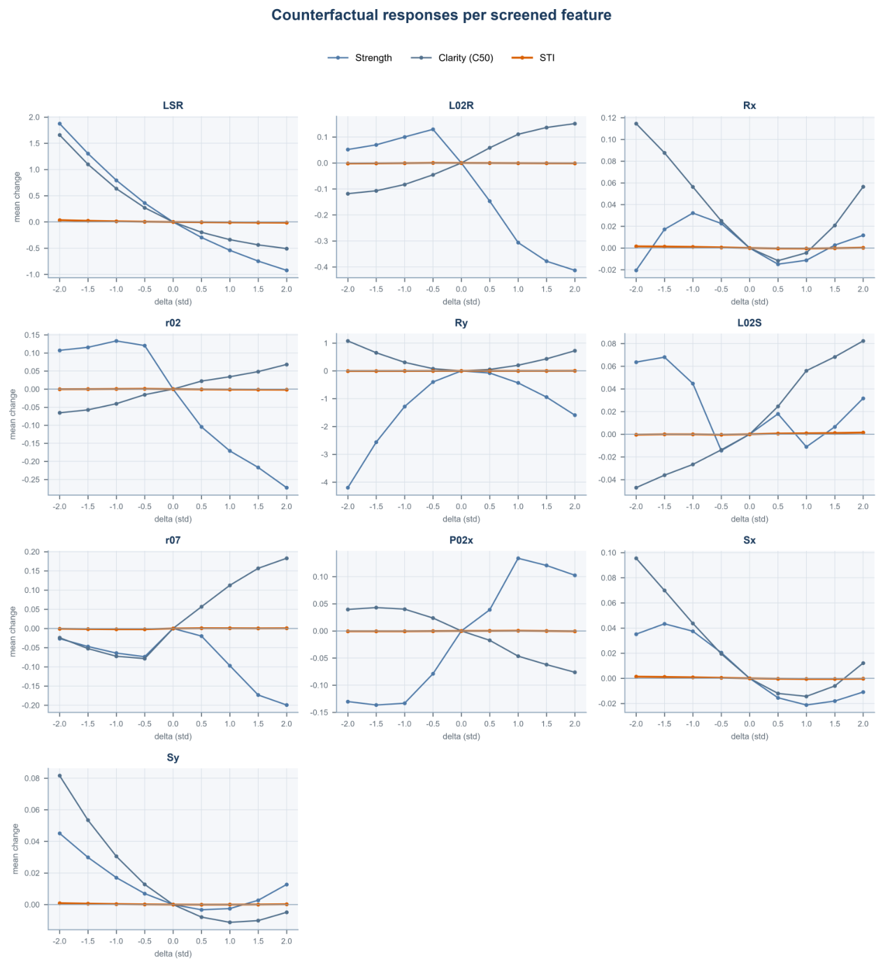
This appendix presents the complete sensitivity results for the screened design variables. Figure A1 summarizes the accumulated local effect curves, while Figure A2 reports the corresponding counterfactual response profiles under standardized perturbations. These figures extend the representative results discussed in Section 3.5.
Figure A1.
Accumulated local effect curves for the screened classroom design variables. Each panel shows the model-derived response of representative STI, Strength, and outputs over the observed range of the corresponding feature.
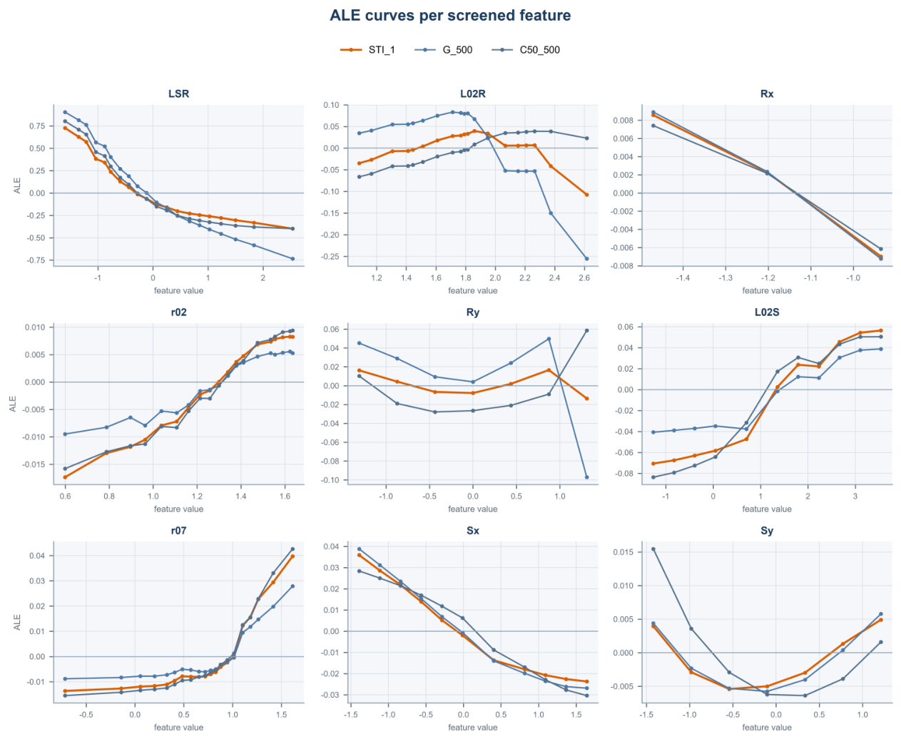
Figure A2.
Counterfactual response profiles for the screened classroom design variables. Each panel shows the mean predicted changes in Strength, , and STI when the corresponding feature is perturbed from to standard deviations relative to the reference condition.
Appendix C. Representative Solutions Under Target-Specific STI Conditions
The following tables report six representative high-quality solutions retained from the target-oriented optimization. Two solutions are shown for each feasible STI target (0.75, 0.80, and 0.85). The solution identifiers are held constant across Table A3, Table A4, Table A5, Table A6 and Table A7, allowing the complete design variables, acoustic predictions, and reliability measures of each solution to be read across the five tables without omitting any values from the original optimization output.
Table A3.
Global design variables and node parameters – for the representative STI-targeted solutions.
Table A4.
Node parameters – and design-change costs for the representative STI-targeted solutions.
Table A5.
Predicted Strength outputs for the representative STI-targeted solutions.
Table A6.
Predicted outputs for the representative STI-targeted solutions.
Table A7.
STI predictions and reliability measures for the representative STI-targeted solutions.
References
- Kaushik, A.; Arif, M.; Tumula, P.; Ebohon, O.J. Effect of thermal comfort on occupant productivity in office buildings: Response surface analysis. Build. Environ. 2020, 180, 107021. [Google Scholar] [CrossRef] [Scilit]
- Jeon, J.Y.; Jo, H.I. Effects of audio-visual interactions on soundscape and landscape perception and their influence on satisfaction with the urban environment. Build. Environ. 2020, 169, 106544. [Google Scholar] [CrossRef] [Scilit]
- Minelli, G.; Puglisi, G.E.; Astolfi, A. Acoustical parameters for learning in classroom: A review. Build. Environ. 2022, 208, 108582. [Google Scholar] [CrossRef] [Scilit]
- Zhang, D.; Tenpierik, M.; Bluyssen, P.M. Individual control as a new way to improve classroom acoustics: A simulation-based study. Appl. Acoust. 2021, 179, 108066. [Google Scholar] [CrossRef] [Scilit]
- Ribeiro, R.S.; Amlani, A.M.; de Conto, J.; Schwerz, B.G.; Amarilla, R.S.D.; Sant’Ana, L.H.; Avelar, M.; Catai, R.E.; Matoski, A. Acoustical treatment characterization of a classroom with wood-based composites. Appl. Acoust. 2021, 178, 107967. [Google Scholar] [CrossRef] [Scilit]
- Cruz, A.; Caldas, L.; Mendes, V.; Mendes, J.; Bastos, L. Multi-objective optimization based on surrogate models for sustainable building design: A systematic literature review. Build. Environ. 2024, 266, 112147. [Google Scholar] [CrossRef] [Scilit]
- Milo, A. The acoustic designer: Joining soundscape and architectural acoustics in architectural design education. Build. Acoust. 2020, 27, 83–112. [Google Scholar] [CrossRef] [Scilit]
- Ma, K.W.; Mak, C.M.; Chung, F.L.; Wong, H.M. Advanced Acoustic Monitoring Using Psychoacoustic Heatmap Machine Learning Models for Noise Impact Prediction in Air-Conditioned Building Environments. Sensors 2026, 26, 544. [Google Scholar] [CrossRef] [Scilit] [PubMed]
- Manesh, M.T.; Dehnavi, A.N.; Tahsildoost, M.; Alambeigi, P. Acoustic design evaluation in educational buildings using artificial intelligence. Build. Environ. 2024, 261, 111695. [Google Scholar] [CrossRef] [Scilit]
- Nannariello, J.; Hodgson, M.; Fricke, F.R. Neural network predictions of speech levels in university classrooms. Appl. Acoust. 2001, 62, 749–767. [Google Scholar] [CrossRef] [Scilit]
- Yeh, C.Y.; Tsay, Y.S. Using Machine Learning to Predict Indoor Acoustic Indicators of Multi-Functional Activity Centers. Appl. Sci. 2021, 11, 5641. [Google Scholar] [CrossRef] [Scilit]
- Lopez-Ballester, J.; Felici-Castell, S.; Segura-Garcia, J.; Cobos, M. AI-IoT Platform for Blind Estimation of Room Acoustic Parameters Based on Deep Neural Networks. IEEE Internet Things J. 2023, 10, 855–866. [Google Scholar] [CrossRef] [Scilit]
- Duangpummet, S.; Karnjana, J.; Kongprawechnon, W.; Unoki, M. Blind estimation of speech transmission index and room acoustic parameters based on the extended model of room impulse response. Appl. Acoust. 2022, 185, 108372. [Google Scholar] [CrossRef] [Scilit]
- van Waterschoot, T. Deep, data-driven modeling of room acoustics: Literature review and research perspectives. arXiv 2025, arXiv:2504.16289. [Google Scholar]
- Scarselli, F.; Gori, M.; Tsoi, A.C.; Hagenbuchner, M.; Monfardini, G. The graph neural network model. IEEE Trans. Neural Netw. 2008, 20, 61–80. [Google Scholar] [CrossRef] [Scilit] [PubMed]
- Wu, Z.; Pan, S.; Chen, F.; Long, G.; Zhang, C.; Yu, P.S. A comprehensive survey on graph neural networks. IEEE Trans. Neural Netw. Learn. Syst. 2020, 32, 4–24. [Google Scholar] [CrossRef] [Scilit] [PubMed]
- Harvie-Clark, J.; Dobinson, N. The practical application of G and C50 in classrooms. In Proceedings of the Inter-Noise and Noise-Con Congress and Conference Proceedings; Institute of Noise Control Engineering: Wakefield, MA, USA, 2013; Volume 247, pp. 1510–1520. [Google Scholar]
- Bradley, J.S.; Reich, R.; Norcross, S. A just noticeable difference in C50 for speech. Appl. Acoust. 1999, 58, 99–108. [Google Scholar] [CrossRef] [Scilit]
- Steeneken, H.J.; Houtgast, T. A physical method for measuring speech-transmission quality. J. Acoust. Soc. Am. 1980, 67, 318–326. [Google Scholar] [CrossRef] [Scilit] [PubMed]
- Tang, S.K.; Yeung, M. Speech transmission index or rapid speech transmission index for classrooms? A designer’s point of view. J. Sound Vib. 2004, 276, 431–439. [Google Scholar] [CrossRef] [Scilit]
- Zhao, J.; Qin, Z.; Ma, B.; Lan, W.; Liu, B.; Pang, S. MTCL-Net: A Multi-Task Contrastive Learning Network for Underwater Acoustic Source Ranging. Remote Sens. 2026, 18, 1343. [Google Scholar] [CrossRef] [Scilit]
- Huang, W.; Sun, S.; Lu, J.; Xu, Z.; Xiu, Z.; Zhang, H. A multi-task learning balanced attention convolutional neural network model for few-shot underwater acoustic target recognition. Expert Syst. Appl. 2026, 313, 131597. [Google Scholar] [CrossRef] [Scilit]
- Linardatos, P.; Papastefanopoulos, V.; Kotsiantis, S. Explainable AI: A Review of Machine Learning Interpretability Methods. Entropy 2021, 23, 18. [Google Scholar] [CrossRef] [Scilit] [PubMed]
- Mehdiyev, N.; Majlatow, M.; Fettke, P. Interpretable and explainable machine learning methods for predictive process monitoring: A systematic literature review. Artif. Intell. Rev. 2025, 58, 378. [Google Scholar] [CrossRef] [Scilit]
- Sun, X.; Yang, Y.; Jia, H.; Zhao, H.; Bi, Y.; Sun, Z.; Yang, J. Acoustic structure inverse design and optimization using deep learning. J. Sound Vib. 2025, 596, 118789. [Google Scholar] [CrossRef] [Scilit]
- Gao, N.; Wang, M.; Cheng, B.; Hou, H. Inverse design and experimental verification of an acoustic sink based on machine learning. Appl. Acoust. 2021, 180, 108153. [Google Scholar] [CrossRef] [Scilit]
- Lee, J.; Park, D.; Lee, M.; Lee, H.; Park, K.; Lee, I.; Ryu, S. Machine learning-based inverse design methods considering data characteristics and design space size in materials design and manufacturing: A review. Mater. Horiz. 2023, 10, 5436–5456. [Google Scholar] [CrossRef] [Scilit] [PubMed]
- Li, J.; Huang, H.; Wang, G. A Small-Sample Prediction Model for Ground Surface Settlement in Shield Tunneling Based on Adjacent-Ring Graph Convolutional Networks (GCN-SSPM). Buildings 2025, 15, 3519. [Google Scholar] [CrossRef] [Scilit]
- Li, Y.; Tarlow, D.; Brockschmidt, M.; Zemel, R. Gated graph sequence neural networks. arXiv 2015, arXiv:1511.05493. [Google Scholar]
- Altman, D.G.; Bland, J.M. Standard deviations and standard errors. BMJ Br. Med. J. 2005, 331, 903. [Google Scholar] [CrossRef] [Scilit] [PubMed]
- Kingma, D.P.; Ba, J. Adam: A method for stochastic optimization. arXiv 2014, arXiv:1412.6980. [Google Scholar]
- Prechelt, L. Early stopping-but when? In Neural Networks: Tricks of the Trade; Springer: Berlin/Heidelberg, Germany, 2002; pp. 55–69. [Google Scholar]
- Chicco, D.; Warrens, M.J.; Jurman, G. The coefficient of determination R-squared is more informative than SMAPE, MAE, MAPE, MSE and RMSE in regression analysis evaluation. Peerj Comput. Sci. 2021, 7, e623. [Google Scholar] [CrossRef] [Scilit] [PubMed]
- Terven, J.; Cordova-Esparza, D.M.; Romero-González, J.A.; Ramírez-Pedraza, A.; Chavez-Urbiola, E.A. A comprehensive survey of loss functions and metrics in deep learning. Artif. Intell. Rev. 2025, 58, 195. [Google Scholar] [CrossRef] [Scilit]
- Lundberg, S.M.; Lee, S.I. A unified approach to interpreting model predictions. Adv. Neural Inf. Process. Syst. 2017, 30, 4765–4774. [Google Scholar]
- Sundararajan, M.; Taly, A.; Yan, Q. Axiomatic attribution for deep networks. In Proceedings of the International Conference on Machine Learning; PMLR: Cambridge, MA, USA, 2017; pp. 3319–3328. [Google Scholar]
- Jain, S.; Wallace, B.C. Attention is not explanation. In Proceedings of the 2019 Conference of the North American Chapter of the Association for Computational Linguistics: Human Language Technologies, Volume 1 (Long and Short Papers); Association for Computational Linguistics: Stroudsburg, PA, USA, 2019; pp. 3543–3556. [Google Scholar]
- Apley, D.W.; Zhu, J. Visualizing the effects of predictor variables in black box supervised learning models. J. R. Stat. Soc. Ser. B Stat. Methodol. 2020, 82, 1059–1086. [Google Scholar] [CrossRef] [Scilit]
- Deb, K.; Pratap, A.; Agarwal, S.; Meyarivan, T. A fast and elitist multiobjective genetic algorithm: NSGA-II. IEEE Trans. Evol. Comput. 2002, 6, 182–197. [Google Scholar] [CrossRef] [Scilit]
- Lakshminarayanan, B.; Pritzel, A.; Blundell, C. Simple and scalable predictive uncertainty estimation using deep ensembles. Adv. Neural Inf. Process. Syst. 2017, 30, 6402–6413. [Google Scholar]
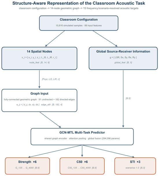
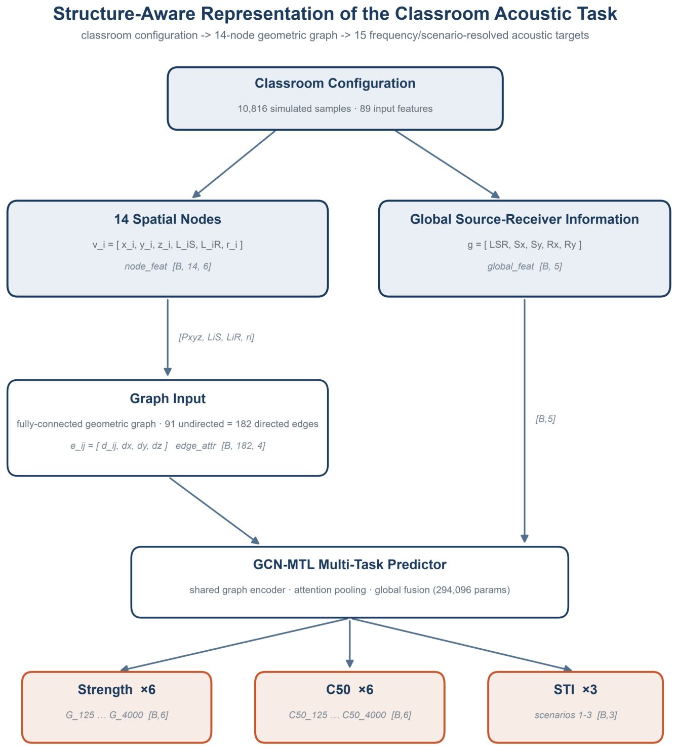
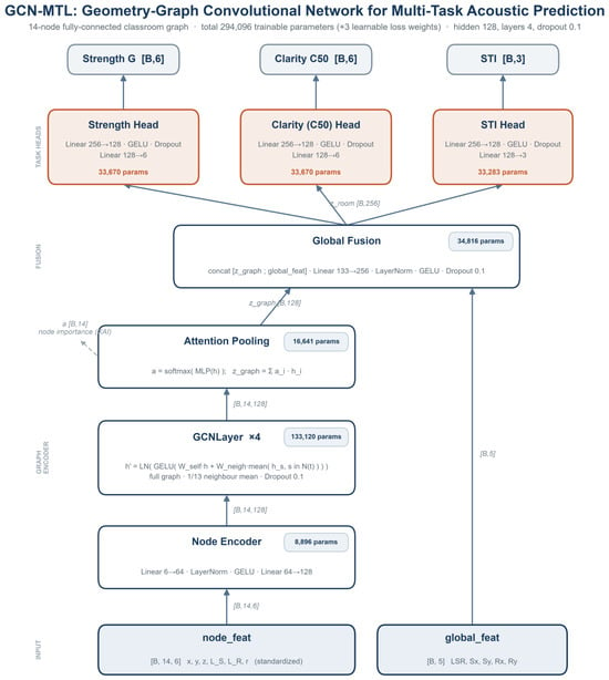
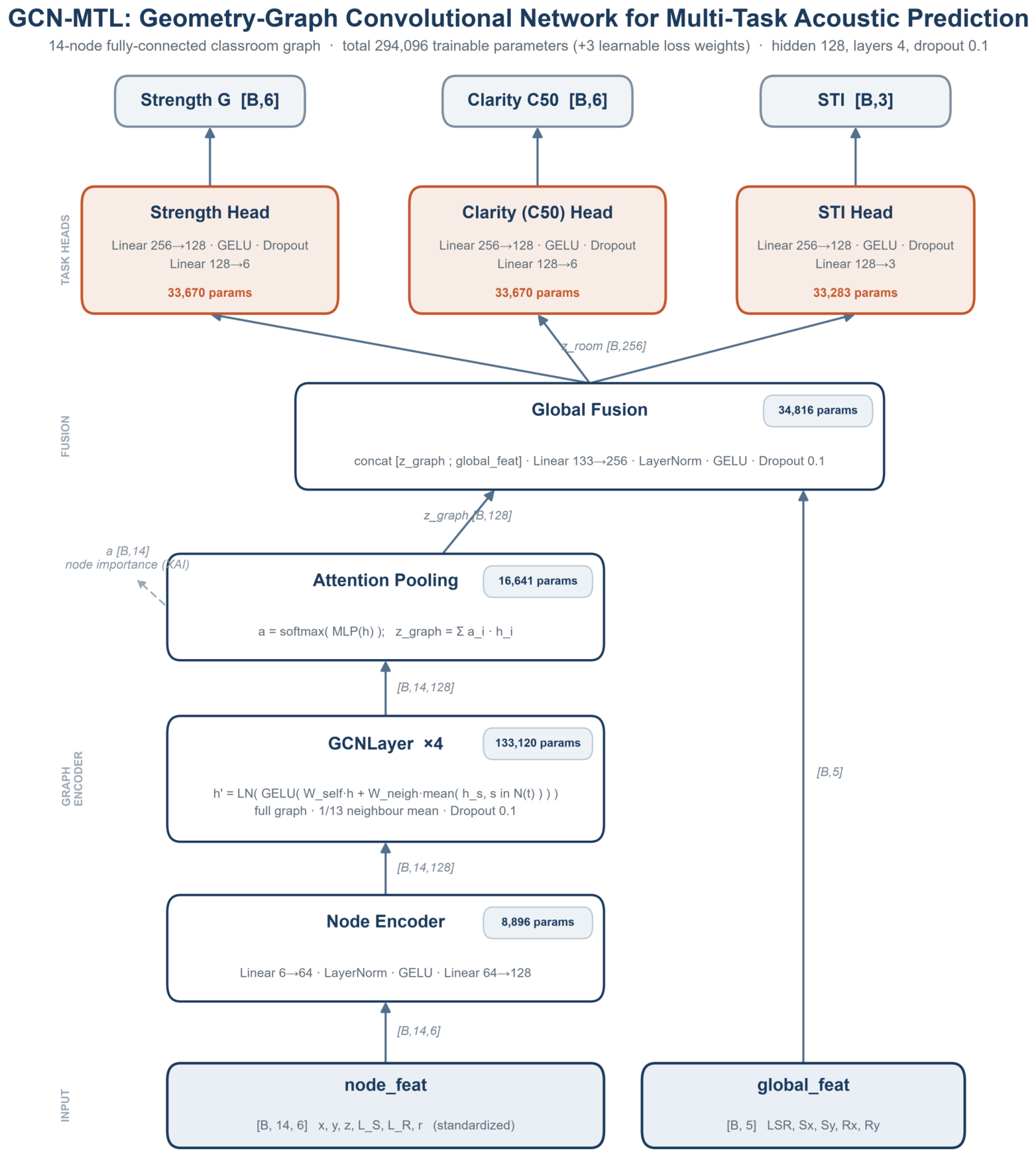
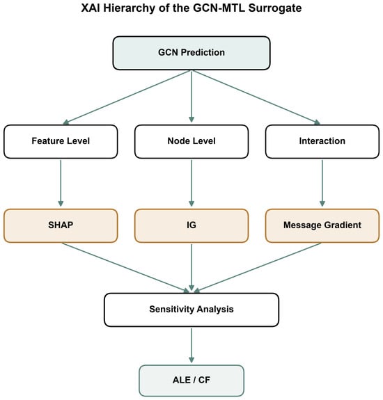
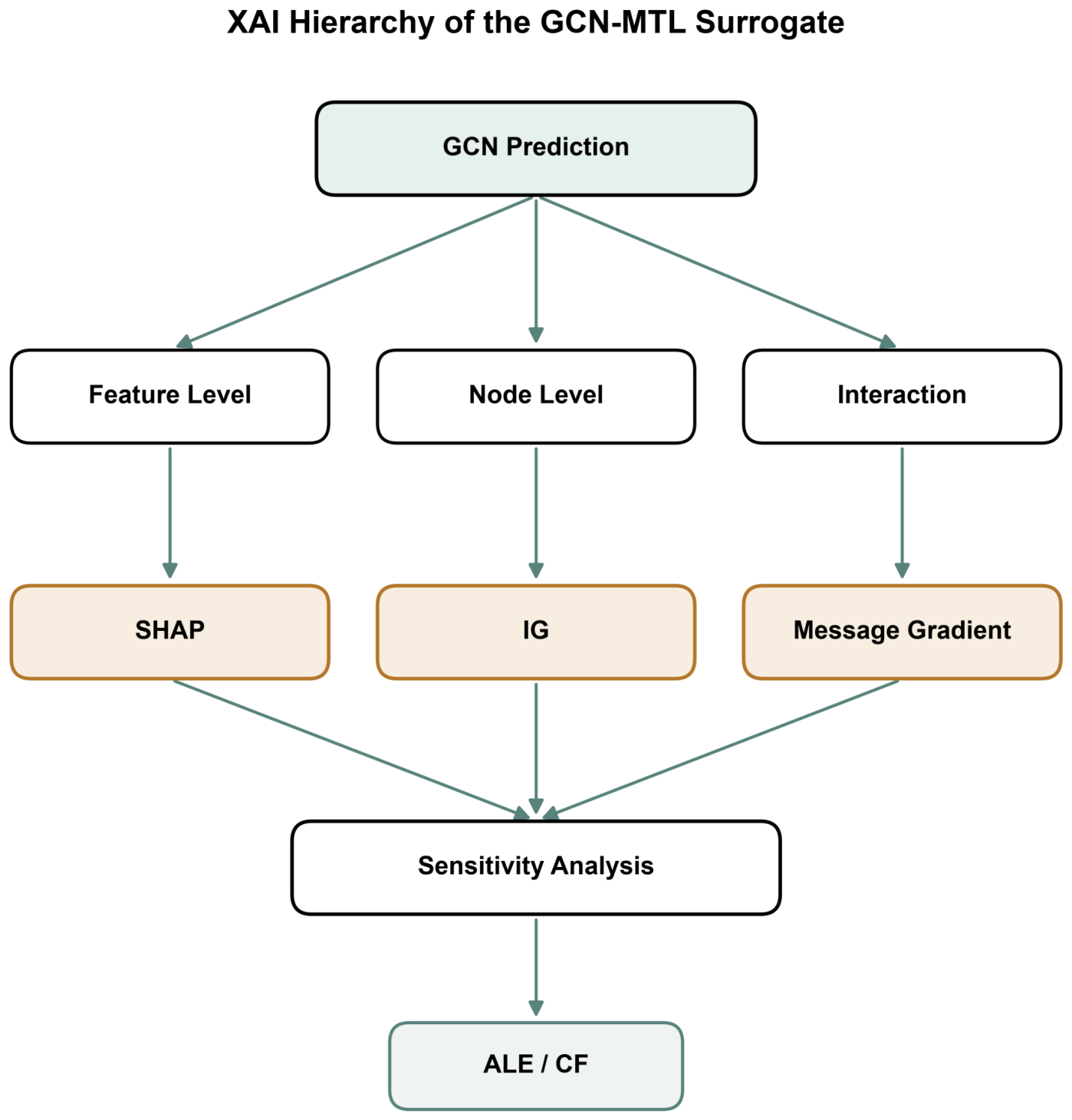
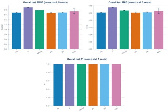
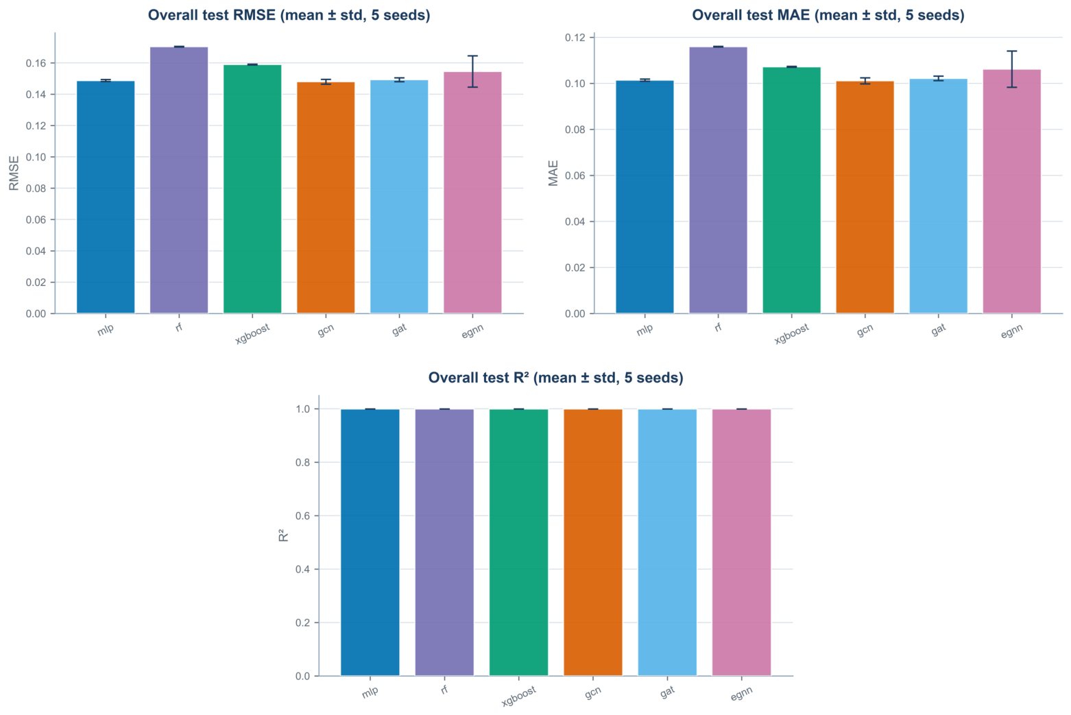
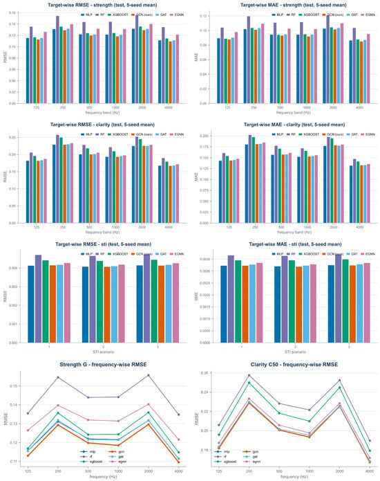
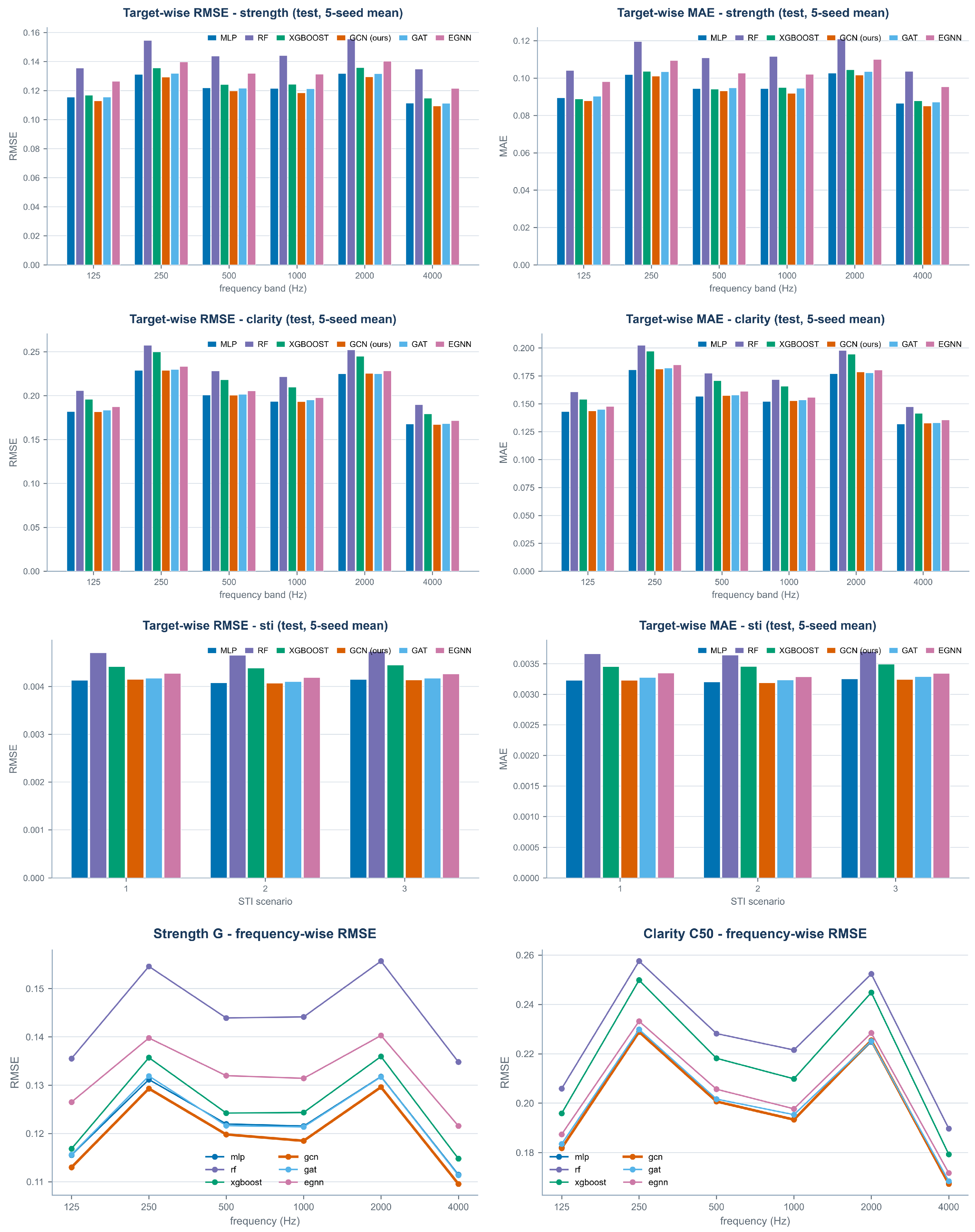
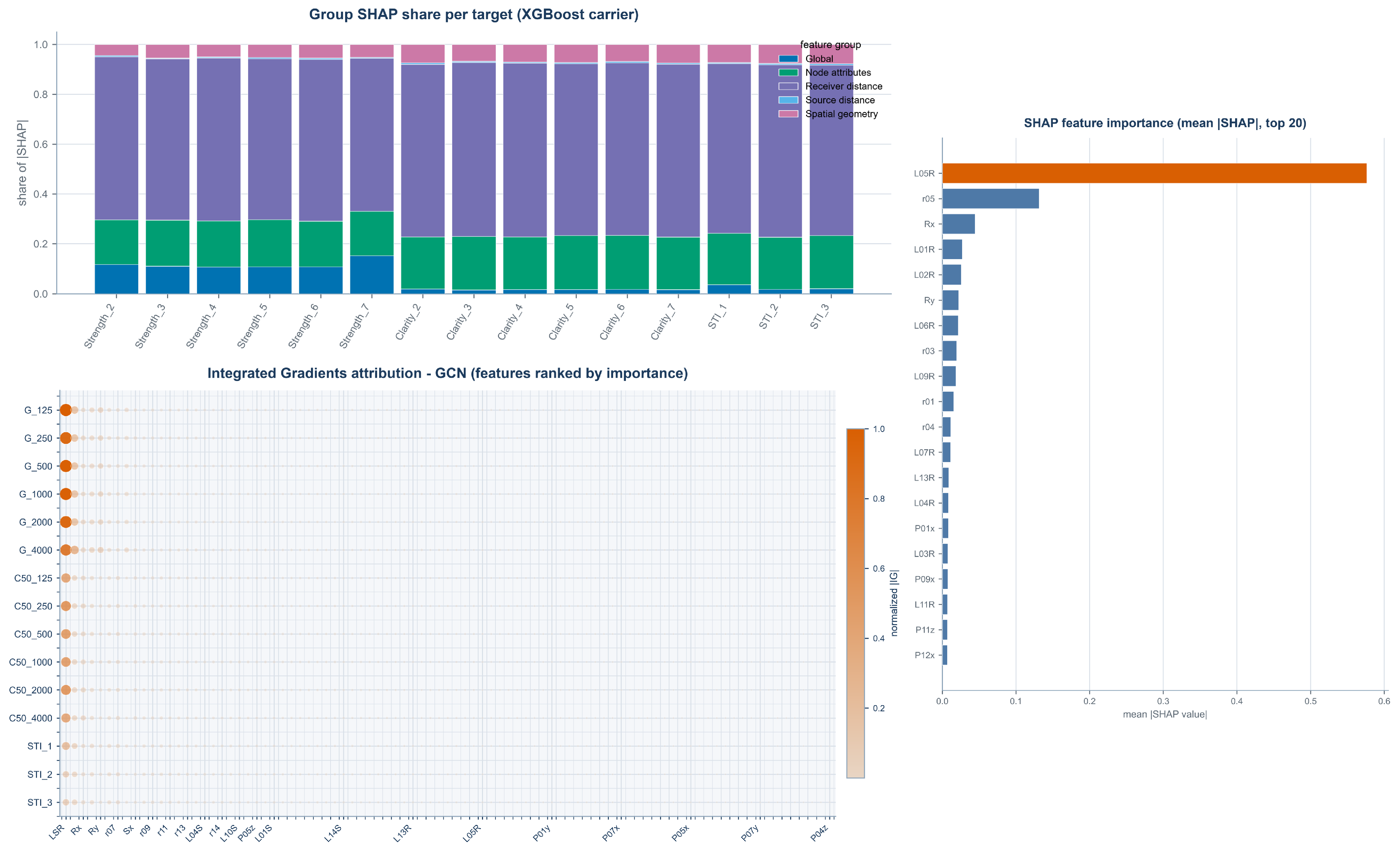
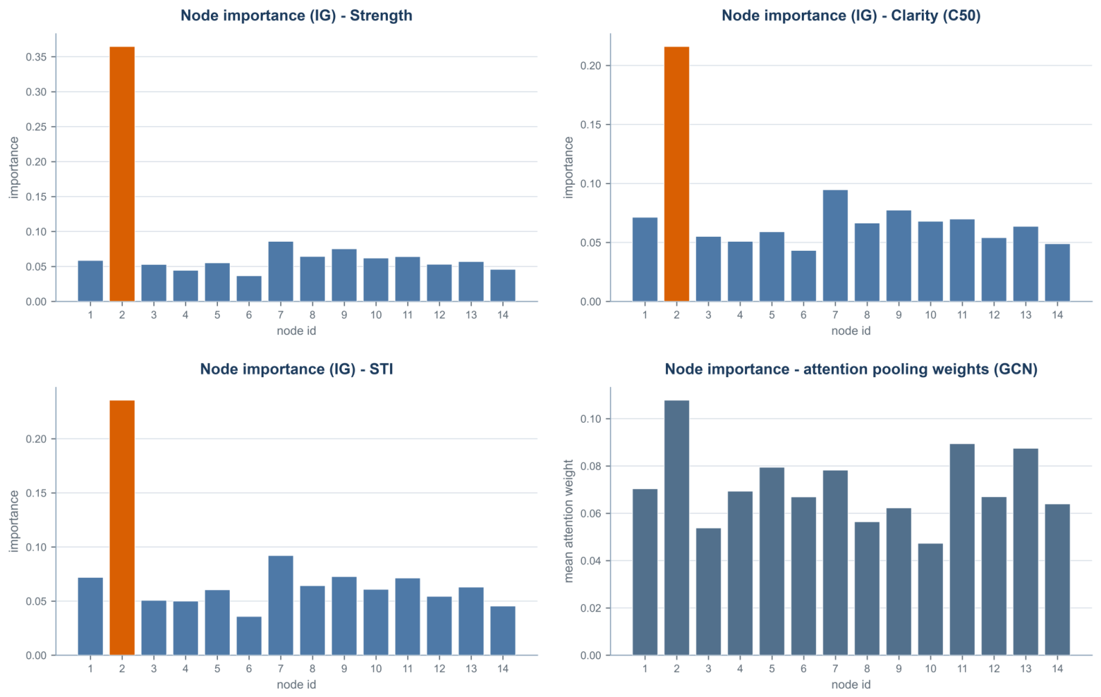
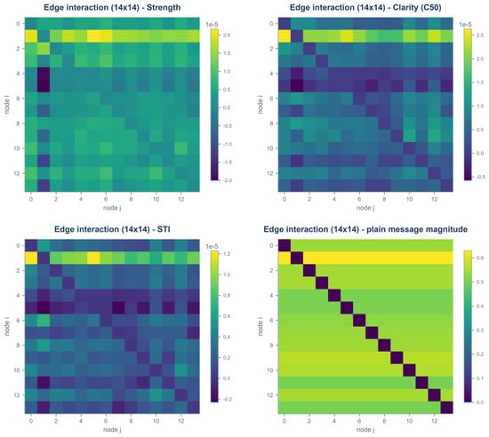
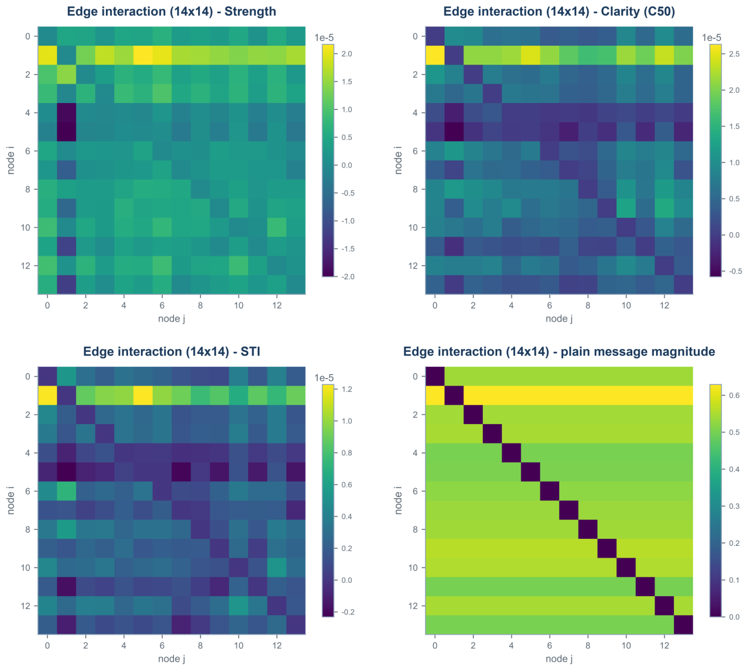
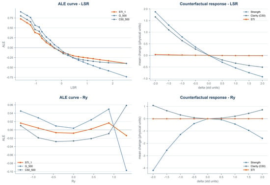
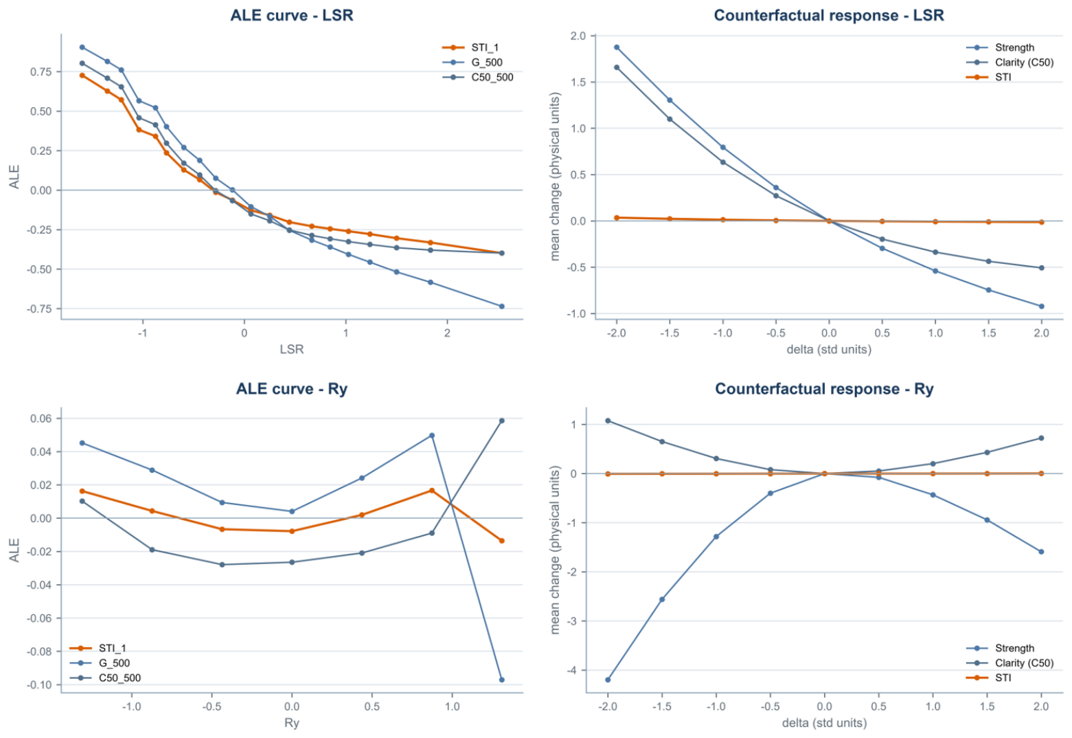
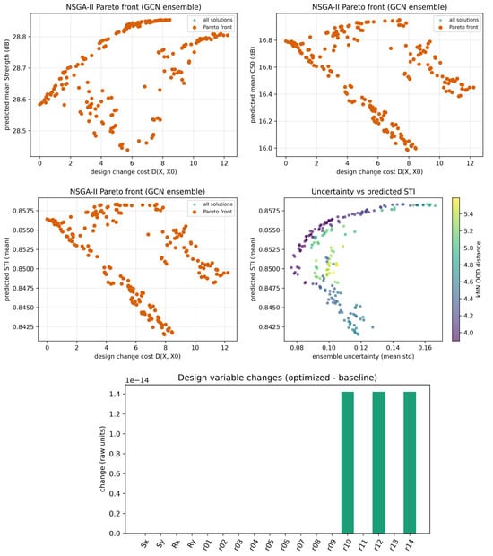
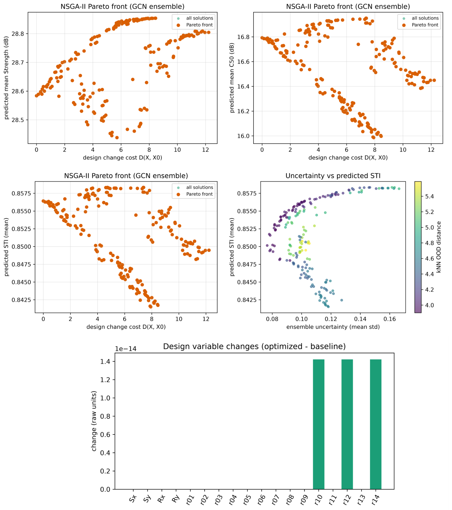

Disclaimer/Publisher’s Note: The statements, opinions and data contained in all publications are solely those of the individual author(s) and contributor(s) and not of MDPI and/or the editor(s). MDPI and/or the editor(s) disclaim responsibility for any injury to people or property resulting from any ideas, methods, instructions or products referred to in the content. |
© 2026 by the authors. Licensee MDPI, Basel, Switzerland. This article is an open access article distributed under the terms and conditions of the Creative Commons Attribution (CC BY) license.