


Abstract
Design errors carried over into construction lead to rework, material waste, and avoidable embodied carbon. Rule-based compliance checking in Building Information Modelling (BIM) can identify explicit design issues. However, current rule-based engines struggle to capture complex spatial arrangements and contextual geometric relationships among surrounding components. Artificial intelligence (AI) offers a promising alternative by learning tacit, geometry-dependent conventions of expert practice directly from BIM data. Yet existing AI approaches either learn from 2D representations or rely on handcrafted geometric features that presuppose the target rules. We conduct a controlled study on a parametric benchmark derived from a single apartment plan. A graph transformer predicts where a masked door belongs along a known host wall. It learns from BIM topology and pose-conditioned neural signed distance function (SDF) embeddings, without explicit coordinate features. On unseen rigid transforms, the model achieves 79.1% side accuracy. A graph attention baseline reaches 68.9%, and a message-passing baseline stays at chance. On a second plan with a different topology, it reaches 68.2%. Doubling the training data does not raise this. Without retraining, the first plan’s model reaches 74.0% on the second. Performance on an unseen room-semantic configuration falls to chance. This is a necessary step towards learning tacit design conventions.
1. Introduction
The sustainability of the built environment is conventionally framed around two carbon accounts: the embodied carbon of the materials that constitute a building [1,2] and the operational carbon consumed over its service life [3,4]. A third account, however, is neither small nor well controlled, namely the material and energy expended during the construction process itself but never embodied in the finished asset [5]. Construction and demolition activities generate one of the largest solid waste streams of any industrial sector [6], yet much of it is not an unavoidable by-product of building but the residue of rework [7,8]. A substantial share of rework originates in the design phase, in the form of design errors, omissions, and late changes [9,10]. The consequences of a design error differ qualitatively from those of an on-site coordination lapse. Once an erroneous specification has propagated to fabrication, components are manufactured with dimensions or interfaces that prevent their installation. The affected elements are then scrapped or stockpiled; replacements are produced from virgin material and transported to the site as an additional delivery. Each of these steps carries its own embodied and transport emissions [7,11,12], so a single error committed at negligible marginal cost in the design office is amplified into a physical and irreversible material loss downstream. Studies of project performance repeatedly identify design-originated defects as a leading contributor to rework cost and, by extension, to avoidable waste [9,13,14]. The quality of the design deliverable is therefore a sustainability variable, not merely a commercial one [15].
Traditionally, design quality is assured through manual review, in which experienced engineers and checkers inspect drawings and models against codes, standards, and established conventions of practice [16]. This mechanism has two structural limitations. First, the resource is scarce and does not scale. Competent review rests on expertise accumulated over years of practice [17], and that expertise is being lost faster than it is replaced [18]. Meanwhile, a single discipline model may carry tens of thousands of components. Second, even unlimited attention would not guarantee correctness because manual checking is labour-intensive and susceptible to human error and oversight [16]. Review is therefore bounded on both sides by how much of a model can be examined and by how reliably any part of it is examined.
Automated compliance checking has become the industry’s expected remedy, and the dominant implementations are rule-based, in that clauses are transcribed into explicit logical or numerical predicates that are then evaluated against the model [19]. This paradigm performs well where the clause is itself explicit and quantitative, for example, a minimum clear width, a maximum travel distance, or a required fire rating [20]. It degrades sharply in two situations. Where a provision is qualitative or discretionary, using terms such as adequate, suitable, or where practicable, there is no faithful translation into a predicate, and the encoding necessarily substitutes the encoder’s interpretation for the clause itself [17,21]. Where a requirement is geometry-dependent, the space of admissible configurations must be enumerated by hand. Because that enumeration is effectively unbounded, any finite rule set covers only the cases its author anticipated [22,23]. Moreover, much of what governs good design is never written down at all. It is a tacit convention, learned by apprenticeship, and thus lies entirely outside the reach of a transcription-based approach [24,25,26]. Rule-based automated compliance checking is consequently accurate but not comprehensive.
Artificial intelligence (AI) offers a complementary route, in that it infers latent regularities directly from data rather than requiring them to be stated in advance. It has demonstrated this capability across domains where the governing rules resist explicit formulation, from architectural layout generation to structure–property relations in materials science that admit no closed-form statement [27,28]. What remains unclear is how the information encoded in digital building data, principally Building Information Modelling (BIM), should be extracted and presented to such a model. One established strategy reduces the three-dimensional model to two-dimensional plan representations [29,30,31]. It applies mature image- or layout-based architectures, which have produced strong results in floor plan generation and analysis. Because the projection discards the geometry that distinguishes one component from another in section and elevation, however, the achievable performance of this family of methods is bounded above by the information the representation retains [32]. A second strategy preserves relational structure by treating the model as a graph and learning over the connections between components with graph neural networks [33,34,35]. Here, the limitation lies not in the topology but in the node features. Attributes are typically hand-specified, so the model is only permitted to discover relationships expressible in terms of quantities that the designer of the feature set already deemed relevant. The representation thereby presupposes the rule to be learned, and correlations lying outside the chosen feature space remain inaccessible [36,37].
This paper addresses that question experimentally. We construct a parametric benchmark from a real apartment model exported to Industry Foundation Classes (IFC), in which a single door is deleted and replaced with a placeholder node carrying no geometry of its own. The position that door should occupy is governed by three predefined placement rules of increasing complexity, namely a threshold rule keyed on the length of an adjacent wall, a label-conditioned chirality rule keyed on the side of the plan a named room occupies, and a relational rule keyed on the position of a uniquely typed window. A graph transformer is then asked to recover that position from the pose-conditioned signed distance function (SDF) embeddings of the surrounding components and the topology of the IFC model alone. No explicit coordinate features are presented as input, although the embeddings are pose-conditioned and therefore encode pose implicitly. Performance is measured only on rigid transforms of the whole plan that were withheld from both embedding fitting and training, so that what is tested is the recovery of relative geometry rather than the recall of a familiar scene.
The rules are predefined by construction: we wrote them in order to generate a decidable ground truth. The study therefore does not show that tacit conventions can be discovered from expert practice. It tests a necessary condition for that goal, namely whether the chosen representation and architecture can support the classes of inference that such conventions demand: reading a derived length against a threshold, reading which side of the plan a labelled space occupies, and composing a correspondence between components. A failure on rules known to be present would make the learning of unwritten rules an unrealistic prospect, and only formally specified rules provide the ground truth and the derivability ceiling against which a learning gap can be measured. The task is also deliberately narrow: it is a single door-placement inference, studied in depth on one apartment topology and repeated on a second (Section 4.11), not design knowledge in general and not a complete design-review workflow (Section 5.2).
The contributions of this study are threefold:
- Methodological. We introduce an evaluation protocol for pure embeddings. It pairs a shortcut audit with a probe-based derivability ceiling to separate the recovery of relative geometry from memorisation and feature leakage, applied to the embedding stage as well as to the graph model. In addition, we build a controlled parametric benchmark. In this benchmark, the model must recover three predefined placement rules (threshold, label-conditioned chirality, and relational) from geometry, topology, and room labels, without explicit coordinate features. Finally, we propose a probe-then-distil procedure that turns this diagnostic ceiling into an effective training intervention. We report uncertainty over the twelve independent holdout transforms and across seeds as two separate sources, with paired tests between models. The core experiment is then repeated on a second apartment plan with a different room and door topology, and a model trained on one plan is evaluated on the other (Section 4.11).
- Technical. We design a transform-invariant output parameterisation, which we selected after systematically falsifying three alternative approaches. Using this parameterisation, a graph transformer learns to infer component placement solely from IFC topology and pose-conditioned neural SDF embeddings. We also incorporate an auxiliary pose-distillation loss, which improves unseen-transform side accuracy by 8.4 percentage points (95% CI 3.7–13.5) over three matched seeds.
- Substantive. We provide controlled evidence that three predefined, geometry-dependent placement rules can be recovered from pose-conditioned three-dimensional geometry and topology under unseen rigid transforms, on the plan studied in depth and, at lower accuracy, on a second plan of different topology, together with a map of where this fails: an unseen room-semantic configuration, near-threshold wall lengths, and rule composition. A model trained on the plan studied in depth also transfers to the second plan without retraining. This is a necessary condition for, rather than a demonstration of, learning tacit design conventions, and it indicates that learned models could complement rule engines for conventions that are hard to transcribe.
The remainder of this paper is organised as follows. Section 2 reviews the related work and states the research gap. Section 3 details the benchmark, representations, architecture, and training protocol. Section 4 reports eleven experiments. Section 5 discusses the implications, the limitations, and the directions they open, and Section 6 concludes this paper.
2. Literature Review
The Introduction identified two limits on current practice: rule-based automated compliance checking reaches only those provisions that can be transcribed into explicit predicates, and the learning-based alternatives proposed so far either discard the three-dimensional geometry that BIM carries or hand-specify the features through which that geometry is read. This section examines the four bodies of work on which those claims rest and closes by stating the three gaps the present study addresses.
2.1. Automated Compliance Checking and the Tacit-Knowledge Bottleneck
Automated compliance checking has evolved along a consistent trajectory: from procedural checks hard-coded to a specific schema, through explicit, machine-interpretable rule representations, to the semi-automated derivation of rules from regulatory text. Ontological formalisation of building data supports the middle of that progression by giving clauses a vocabulary to bind to [38], and natural-language processing now extracts candidate rules from the text of codes themselves, reducing but not eliminating the manual transcription step [39]. The direction of travel across all three phases is the same. Each advance automates more of the work of getting a written requirement into executable form. None of them changes what happens to a requirement that was never written.
Progress across this trajectory is unevenly distributed with respect to the kind of rule being checked. Established classifications of checking rules separate clauses that require only the comparison of a stored attribute from those requiring derived geometry, extended data structures, or a solution procedure of their own, and the proportion of clauses that current tools handle falls sharply along that ordering [40]. The remaining provisions are not simply harder instances of the same problem. A clause requiring a minimum clear width states its own test; a convention holding that a service door belongs at the short end of a corridor, or that a sanitary compartment’s door should not open towards a living space, states no test at all. It is held as practitioner experience and applied without being articulated [24], and there is consequently no text for a transcription pipeline to consume, however capable that pipeline becomes. The bottleneck is therefore one of knowledge rather than of tooling.
Artificial intelligence has entered this pipeline mainly at the text end. A recent review maps AI and large language model (LLM) work on compliance checking since 2022 onto rule interpretation, model preparation, rule execution, reporting, and decision support [41]. Transformer models align IFC concepts with regulatory terms [42]; LLMs combined with deep learning and ontologies interpret clauses and generate checks [43]; and LLMs connected to authoring tools generate the scripts that perform the check [44]. Where LLMs are asked to handle geometry directly, spatial errors appear, and recent frameworks therefore delegate geometric verification to a deterministic kernel [45]. A smaller body of work learns from the model rather than from the text: graph neural networks have been trained to check accessibility requirements from BIM graphs in place of hard-coded rules [46], and semantic alignment by a language model has been combined with graph neural networks to predict the compliance of IFC components [47]. In most of this work, the geometric content of a check is either computed by hand-written procedures or supplied to the learner as engineered attributes. The present study addresses the part these approaches leave open, namely whether the relational geometry on which a placement convention depends can itself be learned from component geometry. It is complementary to them: a learned placement scorer of this kind would sit at the rule-execution stage, beside rule engines, for conventions that have no text to interpret.
Learning the rules from a corpus of designs rather than from a corpus of text is the obvious way past this. It does not, however, dissolve the difficulty so much as relocate it. Once the governing regularity is to be induced from models rather than stated in advance, what determines whether it can be induced at all is how the design is presented to the learner, and that is a question about representation.
2.2. Graph Representations of BIM and Graph Neural Networks in Architecture, Engineering, and Construction
The IFC schema is natively graph-structured. Building products are entities, and the IfcRelationship hierarchy supplies typed relations between them, so graph learning carries an inductive bias that matches the data without requiring it to be reshaped first [34]. Work in this direction clusters into three groups: generative and retrieval models over the adjacency graphs of two-dimensional floor plans [48,49]; classification, enrichment, and completion of IFC elements [36,50]; and space- or graph-level prediction over whole models [51,52]. Two studies sit closest to the present one. BIGNet pretrains a graph network that embeds semantic, spatial, and topological BIM data into reusable node representations [33], and Xiao et al. reason over BIM graphs to automate geometry-intensive compliance checking [23]. Neither poses the question asked here, namely whether relative geometry can be recovered from learned geometric embeddings when coordinates are withheld from the input and evaluation is confined to unseen rigid transforms. The present study is therefore complementary to both, and the protocol of Section 3 could be applied to either.
Across all three groups, component geometry is handled in one of two ways. It is either discarded, leaving the topology and categorical attributes to carry out the task, or supplied directly as coordinates, bounding-box dimensions, or scalar descriptors computed from the solid [51]. Both choices are appropriate to the tasks for which they were made, and the results reported on those tasks are not in question. Neither, however, permits the question asked here to be posed. The first removes the geometric evidence that a placement rule depends on; the second supplies, as an input, the coordinate frame in which the answer is expressed, so a model may reproduce the correct position without performing any spatial reasoning at all. The reported accuracy cannot distinguish the two cases.
Equally consequential is what the evaluation protocols typically omit. Among the works reviewed above, holdouts constructed from rigid transforms of an entire scene are not reported, and neither are audits of the input features for identity leakage. Since BIM datasets are ordinarily derived from a small number of real projects, and the same scene therefore recurs across many training instances, an accuracy figure obtained without those controls cannot separate genuine geometric understanding from memorisation of a fixed scene.
2.3. Neural Implicit Geometry Representations
Neural implicit representations encode a shape as a continuous function rather than as an explicit mesh or point set. The auto-decoder formulation of DeepSDF represents each shape as a latent code optimised jointly with a shared decoder, so that a fixed-length vector stands for a complete continuous surface [53]; occupancy- and radiance-field formulations established the generality of the idea shortly afterwards [54,55]. Multi-resolution hash encodings later reduced the cost of fitting such representations by orders of magnitude [56], which is what makes per-instance encoding of a large component inventory practical rather than merely possible.
Latent codes obtained this way have been used as features for downstream tasks, including shape retrieval and robotic manipulation [57], thereby establishing that they retain geometric information that a subsequent model can act on. Their application to building components is more recent and remains limited [58]. The pose-conditioned auto-decoder used here is the one introduced by the present authors in [58], where it was developed to give IFC components compact geometric descriptors retaining real-world scale, position, and orientation, and was evaluated on the representation of modular components. That work contributed the representation; what the present study adds is the relational question built on it, namely whether many such latents arranged on a graph support inference across components under a protocol that withholds explicit coordinate features, together with the shortcut audit and derivability ceiling that make the answer interpretable. The use of the latents here departs from the wider implicit-geometry literature in two respects, both deliberate. First, components are not normalised to a canonical frame: pose is baked into the latent. This inverts the standard practice of normalising shape before encoding and is why the central question here is empirical rather than assumed; if pose were normalised away and reintroduced as an explicit coordinate, the question of whether the network could recover relative geometry would never be tested. Second, the latents serve as node features supporting relational inference across many components, rather than as a substrate for reconstructing or generating a single shape.
Both departures carry a cost, which we state here. Declining to normalise pose means the encoder must spend capacity representing where a component sits as well as its shape. Hence, reconstruction fidelity per unit of latent width is lower than that which a canonicalised encoder would achieve on the same inventory. That trade is accepted deliberately here: the study measures whether relative geometry can be recovered from the latent, and a canonicalising encoder answers that question by construction rather than by evidence. What the trade forecloses is any claim about reconstruction quality, which is accordingly not among the results reported.
2.4. Graph Transformers, Shortcut Learning, and Evaluation Integrity
Message passing is the default paradigm for graph learning, and its expressive power is characterised by the Weisfeiler–Lehman test [59]. Its practical limitation is over-squashing: information from distant nodes is compressed into fixed-width representations, and adding depth does not reliably relieve the bottleneck [60]. On graphs as small as those used here, reach is not the binding constraint, and Section 4.5 matches it explicitly rather than relying on it. Graph transformers respond by replacing local aggregation with dense attention and reintroducing graph structure through encodings rather than through the message-passing topology. Graphormer combines centrality and shortest-path encodings as attention biases, which makes any pair of nodes reachable in a single attention step [61]. Section 4.5 contributes a controlled instance of this comparison in which the receptive field is explicitly matched, so that reach can be excluded as the explanation of any difference that remains.
A second body of methodological work bears directly on how the present results are to be read. Deep networks frequently succeed by exploiting superficial regularities that correlate with the label but not with the capability being attributed to them, a failure mode documented across vision, language, and scientific applications and termed shortcut learning [62]. BIM data is unusually exposed to this risk for three compounding reasons. Component names routinely carry family identifiers, instance numbers, and, in some export settings, dimensional suffixes; datasets are typically derived from a small number of real projects, so scenes repeat across instances; and coordinates are commonly supplied as node features, as noted in Section 2.2. Each of these, on its own, is a sufficient channel for a model to produce correct answers without performing the reasoning credited to it. The consequence for evaluation is that an accuracy figure is uninterpretable unless the channels through which it could have been obtained have been closed and shown to be closed.
Probing classifiers are the standard instrument for asking whether a given piece of information is present in a learned representation [63]. Still, the method carries a known caveat: linear decodability establishes that information is available, not that the downstream model uses it [64]. The caveat is usually treated as a limitation on what probing can conclude. We treat it instead as a measurement opportunity because the two quantities it separates can both be measured. The gap between a probe-established ceiling and end-to-end performance is itself a number, and it distinguishes a data problem from a learning problem: where the probe reaches a level the trained network does not, the information is demonstrably present, and the shortfall lies in the optimisation rather than in the representation or the benchmark. Since auxiliary objectives are an established means of shaping intermediate representations [65], distilling the readout that the probe indicates turns that diagnosis into an intervention, and the size of the gap it closes is the test of whether the diagnosis was correct.
2.5. Research Gaps
Three gaps follow. First, BIM graph-learning research lacks an evaluation protocol that excludes coordinate inputs and identity leakage, so the reported accuracies cannot distinguish the recovery of relative geometry from memorisation of a repeated scene (Section 2.2 and Section 2.4). Second, it has not yet been verified whether latent representations of neural implicit geometry can support relational inference across multiple components arranged on a graph, as opposed to reconstructing a single shape (Section 2.3). Third, the methodological literature establishes that information demonstrably present in a representation need not be used by the model built on it but offers no closed loop from that diagnosis to a corrective intervention (Section 2.4). This study addresses the three in sequence: a pure-embedding protocol with de-identified features and unseen rigid-transform holdouts applied to the embedding stage as well as to the graph model; a controlled benchmark in which three predefined placement rules of increasing complexity must be inferred from pose-conditioned SDF embeddings and topology; and a linear probe that establishes a derivability ceiling, followed by a pose-distillation auxiliary loss that closes part of the distance to it.
3. Methodology
3.1. Problem Statement and Pipeline Overview
Given an IFC building model in which one door has been removed and replaced with a geometry-free placeholder node, the task is to predict the world position that door should occupy. The prediction must be made from two sources only: learned geometric embeddings of the other components and the topology of the IFC model. Node coordinates are withheld from the input by protocol: no coordinate, bounding-box, or length feature is supplied, although the SDF embeddings are pose-conditioned and therefore encode pose implicitly (Section 3.3).
Formally, each sample is a heterogeneous graph G = (V,E). Every node v ∈ V carries a latent code zv ∈ ℝ128 produced by an SDF auto-decoder (Section 3.3), together with categorical attributes (IFC class, de-identified family name, object type) and no explicit coordinate features. The latent of the target door node is set to zero. The model emits a scalar , which is composed into world coordinates outside the network (Section 3.6).
The pipeline comprises four stages: (1) parametric IFC variant generation and rigid-transform augmentation; (2) SDF sampling and embedding training on the training copies, with the embeddings of the holdout copies fitted afterwards against the frozen decoder (Section 3.3); (3) graph extraction from IFC with write-back of the learned embeddings as node features; and (4) Graphormer training and holdout evaluation. Figure 1 summarises the arrangement and, in particular, the asymmetric role of coordinates: they enter the pipeline solely as evaluation ground truth and as auxiliary training targets, never as model inputs.
Figure 1.
Overview of the four-stage pipeline: parametric IFC variant generation and rigid-transform augmentation; SDF sampling and embedding training on the 149 training copies, with the holdout embeddings fitted afterwards against the frozen decoder; graph extraction with write-back of the learned embeddings as node features; and Graphormer training and holdout evaluation. Coordinates are used only as evaluation ground truth and as auxiliary training targets. (Colors are used for visual clarity/highlighting only).
Scope of the reasoning under test. The benchmark varies pose, room semantics, and component dimensions over a fixed graph skeleton: within a plan, every sample shares the same topology and the same component inventory (in the main plan, 30 to 32 nodes per graph, drawn from an inventory of 52 encoded component instances per transform copy; in the second plan of Section 4.11, 38 to 40 nodes and 60 instances). What is therefore placed under test is relational geometry within a fixed topology, namely the recovery of relative pose, extent, and correspondence between components, evaluated under rigid transforms withheld from both embedding training and graph-model training. Generalisation across differing topologies is tested only in a limited form: Experiment 11 reruns the pipeline on a second plan with a different room and door topology and component inventory and evaluates a model trained on one plan on the other. Generalisation across plan types and real project models is not addressed, and the figures reported below should not be read as applying to arbitrary BIM models. Two further consequences follow. First, the 129,444 graphs (71,877 training, 23,959 validation, 23,960 seen-test, and 9648 holdout graphs; Table A4) are numerous but not independent: they are parametric variants of one base model, and within the holdout, they are clustered by transform, so the effective number of independent holdout units is twelve (Section 3.7). Second, the rigid-transform holdout tests generalisation to unseen pose only; Section 4.9 adds a configuration-level holdout within the same topology, which tests generalisation to unseen room-semantic, metric, and relational configurations and gives a markedly different answer.
3.2. Parametric Benchmark with Three Predefined Placement Rules
Base model and combinatorial sweep. A real apartment model, authored in Revit and exported to IFC, is swept along the axes in Table 1; a second plan, used only in Experiment 11, is described at the end of this section.
Table 1.
The five sweep axes, their state counts, and the resulting graph counts.
The axes are not fully crossed. The window state is swept only in the 16 wall combinations in which neither wall is effective, that is, the case governed by the six-window rule; in the remaining 105 wall combinations, the TYPE2 window is fixed by the hash, and each combination contributes a single graph. Table 2 gives the resulting counts.
Table 2.
How the 129,444 graphs are made up. A wall combination is one of the 11 × 11 pairings of left and right wall length; a wall is effective when it is present and longer than 1 m, which holds for the seven lengths from 1200 to 3000 mm.
The 300 mm step is deliberate: it places several wall lengths immediately on either side of the 1 m rule threshold defined below, which is what makes the failure analysis of Section 4.6 possible.
Three placement rules. The ground-truth door position is a slot along the host wall, parameterised by the along-wall scalar s over six discrete slots, indexed P1 to P6, spaced 0.95 m apart. Which slot is correct is decided by the rules of Table 3. The rules are predefined by the authors to give a decidable ground truth; they are stylised proxies for three kinds of placement convention, not reproductions of real ones (see Relation to practice, below). All three are keyed on whether each variable-length wall is effective, meaning present and longer than 1 m. Figure 2 illustrates the three rules.
Table 3.
The three predefined placement rules, the condition that selects each, and the capability each demands of the model. Shares are of the training data.
Figure 2.
The three predefined placement rules. (a) Single-wall (threshold); (b) semantic (label-conditioned chirality); (c) six-window (relational). Dotted arrows denote decision outcomes as example.
Relation to practice. The rules are stylised rather than realistic, and their status is stated here explicitly. The single-wall rule is, in form, an explicit numerical clause of the kind that rule engines already check. It is included not as an example of tacit knowledge but because the wall length is not an input feature and must be derived from the embeddings, so it tests whether a metric decision can be read out of learned geometry. The semantic rule conditions on a room label that is given as an input, so it does not test semantic inference; it tests whether the model can read which side of the plan a labelled space lies on, the kind of judgement behind wet-area and door-swing conventions [66,67]. The six-window rule requires a correspondence between two components, of the kind that governs the alignment of openings [68,69]. Real conventions are softer than these rules: they have exceptions, they interact, and they often admit several acceptable solutions (Section 5.3). The benchmark therefore measures whether three classes of inference that such conventions need are supported by the representation; it does not claim that the rules themselves are realistic.
Second plan. To test whether the method, rather than a trained model, carries over to a different topology, a second apartment model was authored in Revit from the first and exported to IFC (Section 4.11). It measures 10 m by 12 m and has seven spaces instead of six, 15 walls, 9 doors, and 8 windows, and its door graph differs. In the main plan, spaces 100 and 101 open onto space 102, which reaches the living room 103 only through the target door, and 103 opens onto 104 and 105. In the second plan, the target door joins the living room 103 to a new bedroom 106 that is otherwise reached only from space 101; the corridor 102 is a short passage between spaces 100 and 101, and the living room opens directly onto spaces 100, 104, and 105. The three rules, their components (the two variable-length walls, the two template doors, and the six far-end windows), and the sweep axes of Table 1 are unchanged; the four room-semantic states place the toilet in space 100, 101, 104, or 105, two on the west and two on the east side of the plan. Each copy therefore again yields 804 graphs, now from 60 encoded component instances and with 38 to 40 nodes per graph. The six slots lie 0.99 m apart (0.95 m in the main plan), symmetric about the midpoint of the two template doors, which the data pipeline supplies as the host-wall anchor exactly as in the main plan. The second plan is generated with 81 copies, of which 69 are training and 12 are holdout transforms (55,476 training-copy and 9648 holdout graphs), and with 161 copies (149 training and 12 holdout transforms) as a scale control.
Anti-leakage design. The three measures of Table 4 close the non-geometric channels through which the answer could otherwise reach the model.
Table 4.
Anti-leakage measures.
3.3. Pose-Conditioned SDF Embeddings
The geometry of each component is encoded by an auto-decoder trained on SDF samples drawn from all components of the 149 training transform copies; the 12 holdout copies are handled separately, as described below. Following the auto-decoding formulation of DeepSDF [53] with the multi-resolution hash-grid coordinate encoding of Instant-NGP [56], a shared hash encoding (16 levels, 2 features per level, table size 219, base resolution 16 growing geometrically to 512) feeds a 3-layer multilayer perceptron (MLP) of inner width 128, conditioned on a per-instance latent z ∈ ℝ128. The latents are free parameters optimised jointly with the decoder; the raw coordinate is appended to the grid features so that the network retains a smooth global signal alongside the discrete grid. The encoder is the pose-conditioned auto-decoder introduced by the present authors, as described in Section 2.3. We sample points per component mesh at a fixed density per square metre of surface: 80% are surface samples displaced to small offsets from the surface, and 20% are drawn uniformly within the sampling volume; we compute their signed distances from the mesh with point-cloud-utils.
Inductive fitting of holdout embeddings. The embeddings of the 12 holdout copies are not learned jointly with the decoder. After the decoder is trained on the training copies, it is frozen, and one latent per holdout component is optimised against it using the reconstruction loss alone; no pose-probe or centroid term is applied to holdout components at any stage. A quality gate requires the mean absolute reconstruction error of the fitted holdout latents to stay within 1.5 times that of the training copies (achieved: 0.60 times). The evaluation is therefore inductive at both the embedding and the graph stage. An earlier version of this pipeline trained the auto-decoder jointly on all 161 copies and applied the pose-probe term to the true centroids of the holdout copies, so the holdout embeddings were fitted with access to holdout geometry and pose. All results for the final model, the derivability ceiling, and Experiments 3 and 5 to 11 use the corrected, inductive pipeline; Appendix A.3 compares the two pipelines under an otherwise identical protocol, and every accuracy is lower under the corrected one.
Two design choices depart from common practice and warrant explicit defence. The first is that pose is baked into the latent. Components are not normalised to a canonical frame. Each transform copy’s instances are separate training objects, encoded at their world pose. The latent therefore necessarily encodes shape, size, and pose, a property we verified by confirming that instances of identical shape at different poses receive distinct latents. This makes the latent a complete geometric description, from which downstream relational reasoning is in principle possible, and it converts the question of whether the network can read pose out of the latent from an assumption into the central question of the study.
This departure from canonicalisation is forced rather than elective. The placement rules are defined over relations between components: which wall is longer, which side the toilet occupies, and which of six windows carries the marked type. The quantity the task consumes is therefore precisely the relative pose that canonicalisation discards. A canonicalised encoding would oblige us to reintroduce relative geometry through some other channel, and the only channel available is the coordinates that this study withholds by protocol. Pose-conditioned latents are consequently not a self-imposed difficulty but the sole representation consistent with a no-coordinate input protocol. A light pose-probe auxiliary loss (weight 0.1, a linear head mapping z to the instance centroid) regularises the training-copy embeddings towards pose linearity; it is never applied to holdout copies.
The second choice is a shared coordinate grid that cannot memorise the scene. Because all rotated and translated copies overlap around the origin, the grid is forced to act as a generic encoding of space rather than as a lookup table for one plan. Instance identity therefore lives only in z.
Training is batched SDF regression with a batch of 524k sample points and a learning rate of 10−3 under exponential decay (rate 0.95 every 50 steps). L2 regularisation is applied at 10−4 on the latents and 10−6 on the hash-table entries, the latter pulling sample-free cells towards zero. Training is stopped early when the rolling mean absolute error falls below 0.0045, a threshold reached at epoch 40 when training on the 149 training copies (Appendix A.2). Grid features are held in float32 throughout, since they are sensitive to quantisation noise. The converged latents are written back into the IFC-derived graphs as node features under a “LatentCode” property set.
3.4. Graph Construction and Input Protocol
Nodes are IFC products: walls, doors, windows, spaces, and fixtures. Each transform copy carries 52 SDF-encoded component instances: 31 walls (11 base walls and 20 wall-length variants), 8 windows, 6 doors, 6 spaces, and 1 slab. The inventory holds every instance the sweep of Table 1 can produce, of which any one graph instantiates a subset. A graph instantiates at most one wall-length variant per side, so it carries 30 to 32 nodes and 69 to 75 typed edges, 74 on average. A 32-node graph comprises 11 walls (9 fixed walls and the two variable-length walls), 8 windows, 5 doors (4 real doors and the synthetic target node), 6 spaces together with a virtual exterior-space node, and 1 slab; the count falls to 31 and then to 30 as one and then both variable-length walls become absent. Of the 9648 holdout graphs, 6960 carry 32 nodes, 2400 carry 31, and 288 carry 30. The graphs of the second plan (Section 4.11) use the same node and edge types; each of its copies carries 60 encoded component instances, and each graph carries 38 to 40 nodes. Edges are typed relations taken directly from the IFC relationship hierarchy. Five types are used: SEPARATES, CONNECTS, HAS_DOOR, HAS_WINDOW, and INTERNAL_TO. A wall is linked by SEPARATES to every space it bounds when it bounds two or more, and by INTERNAL_TO to the single space it bounds otherwise; bounding is established by a planar proximity test between the wall faces and the space boundary (within 5 cm), and external walls, identified by Pset_WallCommon.IsExternal, also bound the virtual exterior-space node. HAS_DOOR and HAS_WINDOW link a host wall to the openings it contains, traced through IfcRelFillsElement and IfcRelVoidsElement. CONNECTS links each door and window to the spaces it opens onto, taken from IfcRelSpaceBoundary. Appendix A.4 documents how the graphs are partitioned.
Every node exposes the same attribute record rather than a type-specific one: the SDF latent, which is set to zero for the target door, together with the eight categorical and four numeric fields set out in Table 5. Fields that do not apply to a given node type are zero-filled, so that every node presents an identical, fixed-width record and a single encoder can serve all node types.
Table 5.
The node attribute record. Every node carries the same record; a field that does not apply to a node type is zero-filled rather than omitted.
These fields are heterogeneous in kind and in magnitude: the categorical identifiers are discrete labels carrying no metric, the flag is binary, and the dimensions are millimetre-scale quantities in the thousands. Summing or concatenating them as raw values would therefore be ill-posed, since they share no common unit, and the large-magnitude fields would dominate the node representation. The encoder follows the TabTransformer design [70] and instead treats each field as a separate token: every categorical field receives its own embedding table, and every numeric field its own linear projection followed by layer normalisation, so that all fields enter the node representation at a comparable scale. The pooled output is a 256-dimensional vector, matching the width of the projected SDF latent, to which it is added.
No coordinates, bounding boxes, or wall-length attributes appear anywhere as explicit input features. The only numeric attributes are the nominal dimensions of the door and window families, 850 × 2100 mm and 600 × 1100 mm, respectively; they are identical in every layout of the benchmark, and walls, slabs, and spaces carry zeros in these fields, so no numeric input varies with the quantity to be predicted. Coordinates exist in the data pipeline in exactly two roles. They serve as evaluation ground truth and as auxiliary targets for the pose-distillation loss in Section 3.6. The network never sees them at inference. The protocol is therefore one of inference without explicit coordinate features, not without positional information: the SDF latents are pose-conditioned by design and encode pose implicitly (Section 3.3), and the final model is trained with centroid supervision through the pose-distillation loss, although centroids are never an input.
3.5. Graphormer Architecture
The graph encoder is a standard Graphormer [61]: dense self-attention over all node pairs, with node-centrality (in-degree and out-degree) encodings added to the node representations, shortest-path spatial encodings applied as attention biases, and edge features accumulated along shortest paths.
The configuration is 8 attention heads, 4 Graphormer layers stacked on a 2-layer heterogeneous node encoder, a feed-forward dimension of 512, an edge-feature dimension of 64, a maximum shortest-path distance of 10, maximum in- and out-degrees of 50, and a dropout of 0.1.
The message-passing baseline of Section 4.5 replaces only this encoder. It uses the Graph Isomorphism Network (GIN) extended with edge features (referred to hereafter as GINE [59,71]) at depth 8, with degree-normalised mean aggregation and bidirectional message passing. All GINE results in Section 4.5 use this architecture; the tuning variants are listed there. The node encoder, output head, losses, and data split are left identical, so that the comparison isolates the graph encoder. Mean rather than GIN’s canonical sum aggregation is used because hub nodes in these graphs reach degree 50, at which summed messages overwhelm the input scale of the update MLP; a sum-aggregation variant stalled at the predict-the-mean solution while the Graphormer trained successfully on identical data. A second baseline replaces the encoder with a graph attention network (GAT) [72] in its GATv2 form [73], also at depth 8: local multi-head attention over graph neighbours, with edge features entering the attention keys, which separates attention as such from the dense, structurally encoded attention of the Graphormer. The Graphormer has 15.6 M parameters in total, of which 9.6 M are in the graph encoder; GINE at depth 8 has 8.3 M (2.3 M in the graph encoder), and GAT has 9.9 M.
3.6. Transform-Invariant Output Parameterisation and Auxiliary Losses
The first output component of the model, produced by the head denoted scalar_s, is interpreted as the along-wall scalar . World coordinates are composed outside the model as
where cw is the host wall’s centre and its unit axis, both taken from the public data pipeline rather than predicted. The axis sign is canonicalised rotation-covariantly, by requiring the plan centroid to lie to the left of the axis, so that s is a rigid-transform invariant.
This head is the outcome of the ablation reported in Section 4.1, not an a priori choice. Every head that requires the model to internalise the copy’s global rotation fails on unseen transforms: direct regression of world coordinates, prediction of a 2D offset from the wall centre, and, most instructively, the product-trap variant in which the model must emit and therefore predict the world axis itself. Under the parameterisation of Equation (1), the training loss, mean squared error (MSE) on the composed position, reduces to MSE on s. The distinction from the failed axis-product variant is that the axis enters the composition once rather than twice. Under the axis-product form, in which the composed position is cw + (aw · pred) aw, the axis does not cancel from the loss, and the model must therefore emit a vector aligned with the copy’s world orientation. Under Equation (1), it cancels entirely, and what the model emits is the invariant scalar itself.
Scope of the output. The model therefore does not localise the door in free space. The host wall is identified by the topology, and its centre and axis are supplied by the data pipeline; the model answers a single one-dimensional question: where along an already known wall does the door belong? The correct answer is one of six discrete slots. For the single-wall and semantic rules, only the two end slots occur, so side accuracy on those graphs is a binary decision; only the six-window rule uses all six slots. The millimetre-scale errors reported below describe the precision of this constrained placement, not free three-dimensional localisation, and because a wrong slot misses by a multiple of the 0.95 m slot spacing, the error distribution is bimodal and exact-slot accuracy is a more informative summary than the median (Section 4.6).
The pose-distillation auxiliary loss is formed by a linear head on the final node states, which predicts each real node’s 2D centroid with the synthetic door node masked out. The auxiliary mean squared error, at weight w = 0.3 (Section 4.3 compares it with w = 0), is added to the training loss only; validation, early stopping, and every reported metric remain pure door loss.
The rationale is diagnostic rather than heuristic. A linear probe indicates that a transform-generalising centroid readout is present in the latents, with a mean error of about 9 cm (Section 3.7 and Section 4.2), yet the door loss alone does not cause the network to internalise it. Distilling that readout into the node states makes relative geometry directly available to attention. Because coordinates appear here as targets and never as inputs, the input protocol of Section 3.4 remains intact. The final model is nonetheless trained with centroid supervision, and the protocol is described accordingly (Section 3.4).
3.7. Training and Evaluation Protocol
Optimisation uses Adam with global-norm gradient clipping at 1.0 and a warm-up plus cosine-decay schedule (peak learning rate 2 × 10⁻⁴, warm-up of 10% of total steps capped at 500), batch size 64 with no gradient accumulation, and a cap of approximately 100 epochs under validation-loss early stopping (rolling 5-epoch mean below 10−3, corresponding to roughly 3 cm root-mean-square error). These choices are not incidental: without clipping and warm-up, the identical model oscillates indefinitely at the predict-the-mean saddle. Each configuration is run with seed 42; the final model is repeated with five seeds (42 and 1–4) and its undistilled counterpart with three (42, 1, and 2). Data exceeding the video random-access memory (VRAM) budget is streamed host-to-device per batch. The hardware and software environment, and the wall-clock cost of each pipeline stage, are recorded in Appendix A.
Beyond a conventional 60/20/20 split of seen-transform graphs, the final 12 of the 161 rigid-transform copies are excluded entirely from both SDF decoder training and graph-model training: every graph belonging to those copies constitutes the unseen-transform holdout. All headline results reported in Section 4 are holdout results. Seen-test performance is near-perfect (1–16 mm) in every Graphormer configuration tested and is reported only as a sanity check. Because the seen-test split shares transform copies with the training split, it is not evidence of transform generalisation (Appendix A.4).
The reported metrics are side accuracy (correctness of signs); exact-slot accuracy (nearest of the six slots), the two carrying chance levels of 50% and 16.7%, respectively; median and mean Euclidean error; the share of errors exceeding 0.5 m; and the per-copy distribution of side accuracy across holdout transforms. Uncertainty is reported from two separate sources. Graphs within a holdout transform share its pose and are correlated, so the independent unit of the holdout is the transform, and the effective sample size is 12, not 9648. Cross-transform uncertainty is reported as a cluster bootstrap over the 12 transforms (10,000 resamples, percentile 95% confidence interval, CI) [74]; a naive per-graph binomial interval would be about six times narrower and is not used. Cross-seed uncertainty is reported as the mean ± standard deviation (SD) over independent seeds, with a t-based 95% interval, and differences are given in percentage points (pp). Differences between two models are tested on the 12 paired per-transform accuracies, with an exact two-sided sign-flip permutation test over all 4096 sign patterns and a paired cluster-bootstrap interval of the mean difference; with 12 transforms, the smallest attainable p-value is 2/4096 ≈ 0.0005. The compositional cuts of Section 4.9 compare two subsets within one model and are tested with a paired t-test across the twelve transforms.
Two frozen-model analyses are run alongside training to establish the derivability ceiling that serves as the audit instrument of this study. First, a ridge probe mapping z to the instance centroid is fitted on training copies only and evaluated on holdout copies, where it attains a mean centroid error of 8.7 cm at R2 = 0.9995. Second, a hand-coded pipeline that applies the three rules to the probe centroids, the topology, and the permitted categorical features selects the correct slot on 90.7% of holdout graphs, and on 100% when the true wall lengths are substituted for the probe-derived ones. Because this pipeline already encodes the benchmark rules, the analysis establishes task-specific recoverability by one fixed readout, not a general information-theoretic ceiling: an end-to-end result below 90.7% indicates a learning shortfall relative to this readout.
4. Results
Eleven experiments are reported. Experiments 1 and 2 establish the protocol; Experiments 3 and 4 apply the method-side and data-side levers that produce the final model; Experiment 5 compares architectures; Experiment 6 dissects the residual error correlationally; Experiment 7 probes the resulting hypothesis by intervention while establishing per-rule capability bounds; Experiment 8 separates the contributions of geometry, graph structure, and structural encoding; Experiment 9 tests generalisation to configurations absent from training; Experiment 10 tests robustness to perturbed inputs; and Experiment 11 repeats the core experiment on a second plan topology and tests whether a trained model transfers between plans. Unless stated otherwise, all experiments share the configuration of Section 3. Experiments 3 and 5 to 10 are conducted on the final 161-copy dataset of the main plan, and Experiment 11 on the second plan. Table 6 summarises the series. The head ablation of Experiment 1, the leaked runs of Experiment 2, and the scaling comparison of Experiment 4 were run during development, under an earlier embedding pipeline in which the holdout embeddings were fitted jointly with the training embeddings (Section 3.3); their conclusions concern the output parameterisation, feature leakage, and data scale and do not depend on that detail. All results for the final model, the derivability ceiling, and Experiments 3 and 5 to 11 use the corrected, inductive pipeline.
Table 6.
Overview of the eleven experiments. All metrics are unseen-transform holdout results; uncertainty is reported as described in Section 3.7.
4.1. Experiment 1: Prediction-Head Ablation Falsifies the Coordinate-System Hypothesis
Three prediction heads were retrained on identical embeddings and graphs: absolute, regressing world coordinates directly; offset, predicting the wall centre plus a 2D residual; and an early axis-product variant of scalar_s. All three fall below 0.09 m on the seen test, and all three collapse to 3.4–4.0 m on unseen transforms, a gap of 44–82 times. In every case, the predictions degenerate either to a constant or to an exact mirror of the truth; the axis-product variant attains an s correlation of −0.999, which is to say it learned the answer with the sign reversed. Figure 3 shows the gap between seen and holdout performance for the three heads. Appendix B, Table A5, gives the seen and holdout metrics of all three heads in full.
Figure 3.
Seen-test versus unseen-transform error for the three prediction heads.
The network cannot reconstruct a global coordinate system from pose-conditioned embeddings; it memorises the finite set of training transforms instead. Any output composition that forces the model to read out the copy’s rotation implicitly fails, including multiplication of an invariant scalar by a predicted axis, the product trap, which stalls stochastic gradient descent at the conditional mean. All subsequent experiments therefore adopt the fully transform-invariant parameterisation of Equation (1).
4.2. Experiment 2: Shortcut Audit and the Derivability Ceiling
The first results obtained under the six-window benchmark looked excellent but were misleading: 100% on both the six-window and single-wall rules, alongside exactly chance performance (49.7%) on the semantic rule. That pattern, two rules perfect and one at chance, is itself the diagnostic. An audit of the input features revealed that the categorical Name attribute carried Revit instance numbers and literal _L#### length suffixes, so that the two apparently solved rules were pure vocabulary lookups requiring no geometry at all, while the semantic rule, having no lexical correlate, was left at chance. The 49.7% quoted above is obtained with the magnitude-and-side output head; a second head in use at the time gives 50.0% on the same data, and both give 100% on the other two rules (Appendix B, Table A6).
After de-identification (Section 3.2), the two rules fall to 70.1% and 76.6%, the actual geometric capability at that data scale, while the semantic rule, aided by a doubling of rotation copies, rises to 64.5%, the first above-chance chirality generalisation observed in this study. The leaked runs were conducted at 41 transform copies, giving three holdout transforms, and the de-identified run at 81 copies, giving six, so the comparison is one of pattern rather than of matched samples (Appendix B.2). Figure 4 shows the per-rule breakdown before and after de-identification. Appendix B, Table A6, sets the leaked and de-identified runs side by side.
Figure 4.
Per-rule accuracy before and after removal of identity-bearing categorical features.
The derivability ceiling (Section 3.7) is established on the same de-identified data. Under the corrected embeddings, the ridge probe reaches a mean centroid error of 8.7 cm at R2 = 0.9995 on the twelve holdout transforms, and the hand-coded pipeline consuming probe centroids, topology, and permitted categorical features selects the correct slot on 90.7% of the 9648 holdout graphs (side accuracy 93.8%). The probe is fitted with the coordinate supervision that the model itself is denied, and this is not circular. Linear decodability is a property of the representation, so the probe establishes that the information is present in the model’s own inputs; fitting the decoder that reads it out is a separate act, and one that requires supervision.
How a centroid error of several centimetres translates into rule accuracy depends on which derived quantity a rule consumes. The single-wall and six-window rules turn on whether a variable wall is longer than 1 m, and the pipeline obtains that length from the positions of recovered centroids. A wall’s centroid moves by 0.5 mm per millimetre of length, so a 900 mm wall, 100 mm below the threshold, lies only 5 cm from the decision boundary in centroid space. The probe reads 900 mm walls on average 52 mm too long, and 41.7% of them are classified as effective, whereas walls of 1200 mm are never misclassified. Substituting the true wall lengths while keeping every other probe centroid restores 100%, so the entire shortfall of the fixed readout lies in this one derived quantity; the semantic rule, which needs no length, is reproduced on all of its graphs. Adding Gaussian noise of increasing magnitude to the true centroids shows the same dependence: slot accuracy falls as the noise approaches the centroid margin of the near-threshold walls.
Two findings follow, one negative and one enabling. First, in the absence of a shortcut audit, headline numbers on a BIM learning benchmark say nothing about geometric reasoning; our own first-round results would have been reported as two rules solved. Second, the task is recoverable to 90.7% by a fixed readout of the permitted inputs, so a model without distillation, at about 70% (Section 4.3), falls short because of learning rather than because the information is absent. That conclusion motivates Experiment 3 directly.
4.3. Experiment 3: Pose-Distillation Auxiliary Loss
Since a transform-generalising linear pose readout is demonstrably present in the latents but is not exploited by a model trained on door loss alone, the natural intervention is to distil it. Training with and without the pose-distillation auxiliary loss (w = 0.3 against w = 0), on identical inductive embeddings and graphs and over three matched seeds, gives the results in Table 7. Figure 5 shows the effect on holdout accuracy and convergence.
Table 7.
Pose distillation on (w = 0.3) and off (w = 0) over three matched seeds. All values are unseen-transform holdout metrics on the final 161-copy dataset.
Figure 5.
Effect of pose distillation (w = 0.3 against w = 0) on unseen-transform holdout accuracy over three matched seeds; thin lines are individual seeds and thick lines their means. (a) Side accuracy by rule; (b) six-window exact-slot accuracy. (Line colors distinguish categories; line dimensions, thickness, and end markers (dots/circles) convey no semantic information).
The holdout comprises 9648 graphs over 12 unseen transforms at 161 copies: six-window n = 4608, single-wall n = 2688, and semantic n = 2352. Seeds 3 and 4 of the distilled configuration, which have no undistilled counterpart, reach 81.1% and 78.7% (five-seed mean 79.1% ± 1.8 pp). Early stopping triggers at epochs 42, 50, and 43 without distillation and at 35, 36, and 32 with it.
Distillation raises overall side accuracy in every matched seed by 7.8, 5.1, and 12.3 pp, a mean gain of 8.4 pp. A paired t-test on the three seed-level differences is underpowered (df = 2, p = 0.057); a two-level cluster bootstrap that resamples seeds and, within each seed, the twelve holdout transforms gives a 95% CI of 3.7 to 13.5 pp, which excludes zero. Distillation also accelerates convergence rather than trading accuracy for training time (early stopping at epochs 32–36 against 42–50), and it stabilises the semantic rule, whose side accuracy ranges from 67.1% to 98.2% across undistilled seeds but from 87.5% to 99.7% with distillation. Under the earlier embedding pipeline, the same comparison had suggested a gain of 16 to 18 pp from single runs; the corrected, multi-seed estimate is smaller but statistically robust.
Distilling a probe-indicated readout into the representation is an effective and inexpensive intervention. The recipe it instantiates (prove the ceiling with a probe, locate the gap, then distil it) is transferable beyond this task and is taken up again in Section 5.1.
4.4. Experiment 4: Rotation-Diversity Scaling and the Final Model
Under the earlier embedding pipeline (Section 3.3), holding the configuration fixed at scalar_s with distillation weight 0.3 and scaling the number of rigid-transform copies from 81 to 161 (with holdout transforms scaled proportionally from 6 to 12) moves overall side accuracy from 88.2% to 92.7%. That difference of 4.5 pp rests on single runs and is not interpreted on its own. The two configurations are also evaluated on different holdout draws, six transforms against twelve different ones, so the comparison is between conditions rather than between matched evaluation sets. The effect is carried instead by the tail and the worst copy: the share of errors exceeding 0.5 m falls from 19.3% to 10.8%, and the worst per-copy accuracy rises from 72% to 81%. Returns are visibly diminishing, and per-copy variance remains the dominant source of uncertainty: performance on an individual unseen transform ranges from 80.8% to 100%. Treating the rigid transform as the independent unit, the copy-level mean side accuracy is 92.7% with a bias-corrected bootstrap 95% confidence interval of 89.4% to 95.9% over the twelve holdout copies, and the copy-level mean share of errors above 0.5 m is 10.8% with an interval of 6.4% to 15.4%. Figure 6 shows the per-copy distribution at both scales. This scaling comparison was not repeated under the corrected pipeline; the final configuration uses all 161 copies.
Figure 6.
Per-copy holdout side accuracy at 81 and 161 rotation copies under the earlier embedding pipeline.
This 161-copy configuration, with inductively fitted embeddings, constitutes the final model of the study: over five seeds, its holdout side accuracy is 79.1% ± 1.8 pp (range 77.0–81.1%, t-based 95% CI 76.9–81.3%). For seed 42, which Experiments 6 to 10 analyse, side accuracy is 80.8% (cluster-bootstrap 95% CI 76.3–85.4% over the twelve transforms), exact-slot accuracy is 70.8% (63.7–78.1%), median Euclidean error is 22.2 mm, and the share of errors above 0.5 m is 28.8% (21.5–36.0%); per-rule side accuracy is 71.2/80.8/99.7% for the six-window, single-wall, and semantic rules. The two sources of uncertainty differ by a factor of almost five: side accuracy varies with an SD of 1.8 pp across seeds but 8.5 pp across the twelve holdout transforms (range 67.7–93.4%). An independent retraining with seed 42 reached 79.4%, within the seed spread. Experiments 5 to 10 analyse this model.
4.5. Experiment 5: Message-Passing and Graph-Attention Baselines—A Controlled Architecture Comparison
Only the graph encoder is replaced with GINE at depth 8 (a receptive field that effectively covers the whole graph) with mean aggregation and bidirectional messages. The node encoder, output head, pose distillation, and data split are unchanged, and hyperparameters are selected on validation loss only, never on the holdout. The GINE baseline was tuned in three stages. Eight configurations (learning rates of 2 × 10⁻⁴, 5 × 10⁻⁴, and 10−3 at depths 4 and 8, and two parameter-matched configurations with a feed-forward width of 2048, giving 8.7 M graph-encoder parameters against 9.6 M for the Graphormer) were each trained for 40 epochs, and all eight remained at the predict-the-mean saddle (validation MSE ≈ 4.2). Because the configuration that converged left the saddle only after 36 to 43 epochs, this short sweep shows that no configuration left the saddle early; it does not rank them. The parameter-matched configuration at a learning rate of 5 × 10⁻⁴ was then run to a 300-epoch cap and never left the saddle (side accuracy 50.0% on the seen test and 50.1% on the holdout). Finally, the configuration of the original comparison (learning rate 2 × 10⁻⁴, depth 8, feed-forward width 512) was run to a 200-epoch cap with seeds 42, 1, and 2. As a second family, a graph attention network at depth 8 (Section 3.5) replaces message passing with local attention over the same neighbourhoods, run to a 200-epoch cap with seed 42. Table 8 compares the Graphormer with the converged GINE configuration, and Section 4.8 gives paired tests against every baseline.
Table 8.
Controlled architecture comparison on the final 161-copy dataset. Only the graph encoder differs. GINE is shown in the configuration of the original comparison, run to convergence (seed 42).
The GINE baseline in the configuration of the original comparison leaves the predict-the-mean saddle after 36–43 epochs, where the Graphormer does so within the first 11, and it then converges: it triggers early stopping at epochs 148, 172, and 124 (seeds 42, 1, and 2) and fits the seen test almost perfectly (99.97–100% side accuracy, 2.3–4.9 mm median error). Its failure is therefore not one of optimisation but of generalisation across rigid transforms: on the holdout, its side accuracy is 49.2%, 51.3%, and 50.5% for the three seeds, at chance, and in each seed, four to eight of the twelve holdout copies fall below chance, the whole-copy mirroring signature of Experiment 1. The GAT baseline, which replaces message passing with local attention over the same neighbourhoods, also fits the seen test (100%) but generalises only partly to 68.9% side accuracy (95% CI 64.9–72.8) and 55.6% exact-slot accuracy; it left the saddle only after about 100 epochs and reached the 200-epoch cap without triggering early stopping. The parameter-matched GINE of the tuning sweep, run to 300 epochs, never left the saddle. Figure 7 shows the validation curves.
Figure 7.
Validation curves of the Graphormer (seed 42), the GINE baseline (seeds 42, 1, and 2; seeds 1 and 2 thin), and the GAT baseline (seed 42) on the corrected embeddings, with identical node encoder, losses, and data. All three fit the training transforms; only the Graphormer generalises to the unseen ones (Section 4.5).
Since the receptive field is matched and the fixed readout of Section 3.7 is architecture-independent, the difference lies in how each architecture generalises what it fits. Dense attention with shortest-path and edge-path encodings places multi-hop relations (the toilet’s side, the TYPE2 window’s slot, a wall length against a threshold) one attention hop away and expresses them relative to the graph structure; message passing at the same depth instead fits a solution that is specific to the training transforms, much as the output heads of Experiment 1 did. In paired tests over the twelve transforms, the Graphormer is ahead of GINE on every transform and ahead of GAT on eleven (difference 11.9 pp, 95% CI 8.7–15.3, p = 0.001; Section 4.8). The claim remains bounded to the configurations tested: it is not that message passing cannot solve the task, but that the tuned configurations here did not generalise across rigid transforms. Two earlier GINE configurations (sum aggregation at depth 4, and mean aggregation at depth 8 stopped at 12 epochs) are described in Appendix B.6.
4.6. Experiment 6: Failure Anatomy—Threshold Ambiguity Rather than Rotation Interpolation
Per-graph attribution across all 9648 holdout graphs of the final model (seed 42) yields three findings.
- The failure rate depends on the deciding wall lengths but differs for each rule (Table A7). For the six-window rule, it rises monotonically with the length of the shortest variable wall present, from 6.9% when neither variable wall is present to 40.8%, 56.9%, and 66.1% for 300, 600, and 900 mm; combinations containing a 900 mm wall, 100 mm below the threshold, fail on 65.7% of graphs against 35.1% for combinations without one. For the single-wall rule, it is roughly constant, at 20–25% for every effective-wall length from 1200 to 3000 mm, and for the semantic rule, it is 2.2% at 1200 mm and zero from 1500 mm upwards. In total, 54.1% of all errors above 0.5 m fall in near-threshold configurations (six-window graphs containing a 900 mm wall, or single-wall and semantic graphs whose shortest effective wall is at most 1500 mm).
- When the model fails, it chooses a wrong slot; it does not place the door imprecisely. All 2779 errors above 0.5 m lie in a wrong slot, and two-thirds of them lie on the wrong side; 78.9% come from the six-window rule, 20.5% from the single-wall rule, and 0.5% from the semantic rule. Only 27.9% of wrong-slot predictions are adjacent to the true slot, so most failures are not near misses, and they are concentrated in a few transforms: five of the twelve account for 59.7% of the errors above 0.5 m. A 6 × 6 slot confusion matrix and per-rule side confusion matrices are released with the evaluation reports.
- Rotation interpolation is ruled out. The 149 training copies comprise 148 randomly drawn rotations and the unrotated base plan, and they leave every holdout rotation within 1.55° of some training rotation. Per-copy side accuracy is unrelated to the angular distance to the nearest training rotation (r = −0.13, p = 0.69); the worst copy, at 67.7%, lies 0.80° from a training rotation, while the best, at 93.4%, lies 0.28° away (Table A9). Figure 8 collects the three views of the failure anatomy. Appendix B, Table A9, lists the twelve holdout transforms individually.Figure 8. Failure anatomy of the final model. (a) Slot error rate against the deciding wall’s length, relative to the 1 m rule threshold; (b) slot confusion matrix for the six-window rule (color denotes intensity); (c) per-copy accuracy against angular distance to the nearest training rotation.
Under unseen transforms, the latent-based wall-length readout is biased: read through the probe of Section 4.2, 900 mm walls appear on average 52 mm longer than they are, and 41.7% of them cross the 1 m boundary. For the six-window rule, whose branch requires every variable wall present to be read as ineffective, this is consistent with a failure rate that grows as the wall present approaches the threshold. It does not explain everything: six-window graphs with a 300 mm wall, far from the threshold, still fail at 40.8%, and the flat 20–25% failure of the single-wall rule is unrelated to threshold distance. Both point to interference between the rules in the joint model. In practical terms, errors of this model are concentrated where a hard metric threshold must be read from learned geometry, which is where a deployed scorer would need calibrated uncertainty and deferral to a reviewer (Section 5.2). All of this is correlational evidence; Experiment 7 tests it by intervention.
4.7. Experiment 7: Single-Rule Ablation, Interventional Test, and Capability Upper Bounds
The training pool is partitioned by rule and balanced down to the smallest rule’s size, giving 29,204 graphs each, 24% of the joint model’s training pool. One model per rule is retrained under the identical final configuration, with the inductive embeddings and seed 42, and evaluated on the per-rule holdout subsets, with results comparable graph for graph with those of the joint model. The balancing target coincides with the semantic rule’s total, so the semantically isolated model sees exactly the same semantic graphs as the joint model. That coincidence makes the semantic comparison a controlled contrast, although isolating a rule still changes both the task and the composition of the training data; a volume-matched control is reported below. Table 9 reports the outcome. Figure 9 compares the joint and isolated models rule by rule.
Table 9.
Single-rule ablation. Each isolated model is trained on 24% of the joint model’s training pool and evaluated on the identical per-rule holdout subset.
Figure 9.
Per-rule accuracy of the joint model against rule-isolated models.
- Every rule in isolation is learned to 97.8–98.2% side accuracy from a quarter of the data and transfers to unseen transforms: six-window 97.8% (cluster-bootstrap 95% CI 94.4–100), single-wall 98.2% (97.2–99.3), and semantic 97.9% (93.8–100). The two rules that are weakest in the joint model recover the most: the six-window rule from 71.2% and the single-wall rule from 80.8%. The semantic rule, already at 99.7% in the joint model, does not improve, and its isolated errors are spread evenly over wall lengths and concentrated in a few transforms rather than near the threshold (Table A7). The joint model’s shortfall therefore reflects the cost of rule composition, not the difficulty of any individual rule.
- The threshold mechanism is supported by intervention. In the joint model, the six-window failure rate rises from 6.9% with no variable wall present to 66.1% when the shortest wall present is 900 mm; in the isolated six-window model, it is flat at 6.9–8.3% across the same groups, and the single-wall failure rate falls from 20–25% to 0–5% (Table A7). We call this interventional rather than causal evidence because isolating a rule changes both the task and the composition of the training data. The data-volume component of that confound is controlled directly: a fourth model, trained on a random mixed-rule sample of the same 29,204 graphs, reaches 80.6% holdout side accuracy (median error 27.7 mm), indistinguishable from the full joint model. Matching the data volume while keeping the rules mixed therefore reproduces the joint model, whereas isolating a rule removes most of the error, which locates the gain in the removal of rule composition rather than in the change of data volume. Figure 10 contrasts the joint and isolated error rates, and Appendix B gives the curves for all three rules (Table A7) and the training scale and seen-test behaviour of the isolated models (Table A8).Figure 10. Slot error rate against the deciding wall’s length: joint model versus rule-isolated models.
- Data volume and rule discrimination are distinct axes. The isolated single-wall and semantic models place the door less precisely within the correct slot than the joint model (median errors of 23.4 and 21.8 mm against 14.6 and 12.1 mm) because they train on fewer graphs; what joint training costs is rule discrimination, not positional precision.
The residual error of the joint model is therefore located in rule selection under composition, which depends on reading derived lengths near the threshold. The targeted next step, outside this paper’s scope, is a length- or extent-distillation auxiliary head structurally analogous to the pose distillation of Section 3.6.
4.8. Experiment 8: Where the Performance Comes from
Four ablation arms separate the contributions of geometry, graph structure, and the Graphormer’s structural encodings, holding the embeddings, schema, training protocol, and seed fixed; together with the architecture comparison of Experiment 5 and the distillation comparison of Experiment 3, they separate representation, architecture, and optimisation effects. In the topology-only arm, every SDF latent is zeroed while the categorical attributes and the real graph links are kept. In the geometry-only arm, the latents are kept, but the links are replaced with a uniform, fully connected structure over the same nodes, so that the centrality and shortest-path biases carry no information. The categorical-only arm removes both. The structural-encoding arm keeps real geometry and real structure but removes the shortest-path and edge-path attention biases. Table 10 reports these arms alongside the architecture baselines, each as a paired comparison with the final model over the twelve holdout transforms.
Table 10.
Paired comparison of the final model with every ablation and baseline arm on the twelve unseen transforms (seed 42 unless stated). Differences are final model minus arm, in percentage points.
Geometry is necessary and carries most of the performance. With real latents but no informative structure, the model reaches 73.6%, whereas with real structure but no geometry, it reaches 55.1% on the holdout despite 71.2% on the seen test, and without either, it is at chance. Graph structure adds a real increment over geometry alone (+7.2 pp), of which the specific shortest-path and edge-path encodings account for a smaller part (+5.2 pp for seed 42, +3.5 pp against the five-seed mean). Architecture matters beyond these components: a local attention encoder with access to the same geometry and structure reaches 68.9%, and message passing, although it fits the seen test, does not generalise at all (Section 4.5). Pose distillation, an optimisation-side intervention on the same architecture and representation, accounts for 7.8 pp for this seed (Section 4.3).
4.9. Experiment 9: Compositional Holdout Within the Fixed Topology
The rigid-transform holdout of Section 4.1 to Section 4.8 withholds pose, but every room-semantic state, wall-length pair, and window configuration appears in training under other poses. To test generalisation to configurations absent from training, three models were retrained with one configuration withheld from the training data entirely, and each was evaluated on the standard twelve-transform holdout, split into graphs with the withheld configuration and graphs with trained ones. The metric cut withholds the length pair 1500/2100 mm and its mirror, which fall under the semantic rule; the relational cut withholds the configurations in which the TYPE2 window occupies slot 3; the semantic cut withholds room-semantic state 4, in which the toilet occupies space 105. Table 11 reports the outcome.
Table 11.
Compositional holdout. Each model is trained without one configuration and evaluated on the twelve unseen transforms; side accuracy with cluster-bootstrap 95% intervals.
Generalisation beyond the pose holdout is uneven. An unseen length combination is handled at least as well as trained ones, so the threshold judgement transfers to new lengths. An unseen window configuration costs 16.8 pp but stays well above chance. An unseen room-semantic state falls to chance: the model does not transfer its reading of which side a labelled space lies on to an arrangement of rooms it has not seen, which indicates that its solution is tied to the room-semantic configurations seen in training. The rigid-transform holdout cannot detect this because every room state appears in training under other poses. The headline results of this paper therefore establish generalisation to unseen pose within a fixed topology, not to unseen semantic configurations and not to new designs (Section 5.3).
4.10. Experiment 10: Robustness to Perturbed Inputs
The benchmark is regular, whereas real models contain noise and missing elements. To test sensitivity to such imperfections, the final configuration was retrained with seed 42 and, in the same process, evaluated on the clean holdout and on five perturbed copies of it: Gaussian noise added to every latent except that of the target node (σ = 0.05, 0.1, and 0.2, about 25%, 50%, and 100% of the latent standard deviation), and random deletion of 10% or 20% of the non-target nodes together with their links. The clean evaluation of this independent retraining reaches 79.4%, within the seed spread of Section 4.4. Table 12 reports the outcome.
Table 12.
Holdout performance of the final configuration under test-time perturbations (seed 42, independent retraining).
Performance degrades gradually rather than collapsing. Noise at a quarter of the latent scale costs 3 pp, and noise as large as the signal leaves 63.5%, still above chance. Node deletion is more damaging because a deleted node may be the host wall, an effective wall, or the marked window on which the rule depends, which removes the evidence rather than blurring it. The test covers noise and missing components only; distractor components, modelling inconsistencies such as misclassified or duplicated elements, and genuinely ambiguous configurations were not generated and remain untested (Section 5.3). As a first step towards uncertainty handling, the five seeds of the final model were combined by majority vote, which reaches 80.6% against a single-seed mean of 79.1%; disagreement between seeds correlates only weakly with error (r = 0.19), so it is not yet a reliable signal for deferring uncertain cases to a reviewer.
4.11. Experiment 11: A Second Plan Topology
Experiments 1 to 10 use one plan, so they cannot separate what the method does from what one topology allows. Experiment 11 asks two questions on the second plan of Section 3.2 (Figure 11). The first is whether the method replicates on a different topology. The complete pipeline is rerun on the second plan without any change of hyperparameters: the SDF decoder is trained on the 69 training copies, the holdout latents are fitted afterwards against the frozen decoder, and the final Graphormer configuration, with pose distillation at w = 0.3, is trained with seeds 42, 1, and 2, together with an undistilled control (w = 0, seed 42). The second question is whether a trained model transfers between plans. The two plans have separately trained decoders whose latent spaces are not aligned, so the twelve holdout copies of the second plan are fitted against the frozen decoder of the main plan instead; the final configuration of the main plan is then retrained (seed 42) and evaluated, in the same process, on its own holdout and on these 9648 graphs. Room labels and component types of the second plan that do not occur in the main plan, such as the corridor, are encoded as unknown categories.
Figure 11.
The second plan. (a) Layout with spaces 100 to 106, the two variable-length walls, the six far-end windows, and the six slots on the host wall of the target door. In each room-semantic state, the toilet occupies one of spaces 100, 101, 104, and 105, and the other three are stores. (b) Door graphs of the main and the second plans. The dashed edge is the target door. (Colors visually link corresponding elements between the floor plan and the graph).
The second plan is run at 81 copies, half the scale of the main plan, so its accuracy is not directly comparable with 79.1%: under the earlier pipeline, halving the copies lowered side accuracy from 92.7% to 88.2% (Experiment 4). A run at 161 copies (seed 42), with 149 training and 12 newly drawn holdout transforms, controls for scale. Embedding quality is not a confound: the fitted holdout latents of the second plan reach 0.61 times the training reconstruction error against its own decoder (0.58 at 161 copies; 0.60 for the main plan) and 0.68 times against the main plan’s decoder, within the quality gate in both cases. Table 13 reports the outcome.
Table 13.
The second plan topology. Holdout metrics on twelve unseen transforms, with cluster-bootstrap 95% intervals in brackets; per-rule side accuracy in the order six-window/single-wall/semantic.
The method carries over, at lower accuracy. On the second plan, the final configuration reaches 68.2% ± 3.6 pp side accuracy over three seeds (seed 42: 67.0%, 95% CI 61.2–72.4; exact slot 43.2%) while fitting the seen test to 100%. Per-transform side accuracy for seed 42 ranges from 49.9% to 80.5% (SD 10.4 pp), against 67.7–93.4% in the main plan. The shortfall is one of generalisation to unseen transforms, not of fitting, but unlike GINE in Section 4.5, the model stays well above chance. Pose distillation adds 7.8 pp on this plan over three seeds (95% CI 3.1–12.6; p = 0.0098), against 8.4 pp in the main plan. The loss is also distributed differently. In the main plan, the semantic rule was almost solved (99.7%), and the error lay in the six-window and single-wall rules near the threshold; on the second plan, the semantic rule falls to 69.6% for seed 42, level with the six-window rule (69.8%), and the single-wall rule is lowest at 59.9%. The semantic loss is one-sided: for seed 42, the rule is solved when the toilet lies on the west side of the plan (89.8% and 95.2% for spaces 100 and 104) and at chance when it lies on the east side (47.3% and 46.3% for spaces 101 and 105). Seed 1 shows the same pattern, and seed 2 is better on the east side (76.2% and 70.6%), but its accuracy is still lower than on the west side. Per-transform accuracy is not significantly related to the angular distance to the nearest training rotation (r = −0.14 to −0.42 over the three seeds, p ≥ 0.18).
A model trained on the main plan transfers to the second plan without retraining. Retrained with seed 42, the final configuration of the main plan reaches 81.6% on its own holdout, close to the 80.8% of the original seed 42 run. On the holdout of the second plan, it reaches 74.0% side accuracy (95% CI 71.5–76.9) and 58.7% exact-slot accuracy. This is above all three models trained on the second plan itself. The gain lies in the semantic rule. The transferred model predicts the correct side on every semantic graph, whereas the models trained on the second plan reach 66.1–81.3% on this rule. The semantic rule can therefore be read on the second topology, and the semantic losses above are not caused by the topology itself. The six-window and single-wall rules reach 64.7% and 67.3%, close to those of the models trained on the second plan (67.5–69.8% and 59.9–69.4%). This test cannot tell whether these two rules are harder on the second plan or are affected by the unknown categories and the different geometry. Placement is also less precise. The median error is 0.14 m, against 9 mm on the main plan’s own holdout.
The embeddings carry over between the plans. The main plan’s decoder reconstructs the components of the second plan about as accurately as its own decoder does (0.68 against 0.61 times the training error). The model therefore meets familiar component geometry in a new arrangement of rooms and doors, and it still reads the rules in most graphs. Two caveats apply. The main-plan model was trained on 149 copies, about twice the 69 copies of the second-plan models. The two plans also share their rule components because the second was derived from the first.
At 161 copies, the scale of the main plan, the second plan reaches 64.4% (seed 42, 95% CI 58.6–69.9). This is no higher than the three seeds at 81 copies (65.3–72.2%). It is 16.4 pp below the 80.8% of the main plan for the same seed. More training transforms therefore do not close the gap. The model trained on the main plan reads the semantic rule on the second plan without error. The second topology therefore does not stop the rules from being read. The shortfall comes from training on the second plan, and this study does not show why.
Experiment 11 thus shows that the method, retrained on a different topology, recovers the three rules above chance but below the main plan, even at equal scale. It also shows that a model trained on the main plan transfers to the second plan without retraining. Two plans, the second derived from the first and sharing its rule components, are not a sample of plan types; the experiment bounds the topology claim rather than establishing generalisation across buildings (Section 5.3).
4.12. Summary of Findings
Capability boundary. Under a strict pure-embedding protocol with shortcut auditing, a Graphormer cannot rebuild a global coordinate frame from pose-conditioned embeddings (Experiments 1 and 2). Given a transform-invariant output parameterisation and inductively fitted embeddings, however, it recovers the three predefined placement rules on unseen rigid transforms at 79.1% ± 1.8 pp side accuracy over five seeds and 70.8% exact-slot accuracy (Experiment 4), against 90.7% for a fixed readout of the same inputs (Experiment 2). The host wall is identified by topology, and its centre and axis are supplied by the data pipeline (Section 3.6), so every positional error reported in this paper is the composition of a one-degree-of-freedom prediction along a known line.
Method. Pose distillation transfers a probe-indicated linear readout into the representation for a gain of 8.4 pp (95% CI 3.7–13.5, three matched seeds; Experiment 3).
Architecture. With the node encoder, losses, and data held fixed, a GINE baseline either stays at the predict-the-mean saddle (eight short configurations) or, once converged, fits the training transforms almost perfectly (99.97–100%) while remaining at chance on unseen ones (49.2–51.3% over three seeds); a GAT baseline reaches 68.9%, and the Graphormer is ahead of both on 11 or 12 of the 12 transforms (Experiments 5 and 8). We do not claim that message passing is incapable of the task, only that under these configurations, it did not generalise across rigid transforms.
Error attribution. Correlational (Experiment 6) and interventional (Experiment 7) evidence locate the residual error in rule selection under composition, which depends on reading derived lengths near a hard threshold; a volume-matched control rules out data volume as the explanation. Per-rule capability is 97.8–98.2% at 24% of the data.
Sources of performance. Geometry is necessary and carries most of the performance, graph structure adds a real increment, and the specific structural encodings add a smaller one (Experiment 8).
Scope of generalisation. Generalisation to an unseen length combination is complete, to an unseen window configuration partial, and to an unseen room-semantic state absent, so the headline results hold for unseen pose, not for unseen semantic configurations (Experiment 9). Performance degrades gradually under latent noise and more sharply when components are missing (Experiment 10). On a second plan topology, the method, retrained from scratch, reaches 68.2% ± 3.6 pp, below the main plan even at equal scale, and a model trained on the main plan reaches 74.0% on the second plan without retraining (Experiment 11).
Honest evaluation. Leakage checks must cover every stage that is trained, including representation learning, and uncertainty must be reported over the twelve independent transforms and across seeds as separate sources; a per-graph count or a two-run noise band overstates the evidence on a holdout of this size.
5. Discussion
5.1. Implications for Learning Design Knowledge from BIM
The three placement rules are stylised, predefined proxies, one rule for each of three kinds of judgement a reviewer makes in practice: whether a dimension passes a threshold, which way a component should face, and whether two components agree with one another. All three can be recovered from pose-conditioned geometry, topology, and room labels without explicit coordinate features, with 97.8–98.2% side accuracy when each rule is learned on its own and 79.1% when the three are learned jointly, under unseen pose within one topology; rerun on a second topology, the method reaches 68.2% (Section 4.11).
This needs to be stated precisely because the natural paraphrase overstates it. The study shows that a model of this kind can support three classes of inference that tacit conventions demand. It does not show that tacit rules have been discovered: the rules used here were written down in advance so that the ground truth would be decidable, for the reasons given in the Introduction. The title accordingly speaks of predefined rules, and the task is one door-placement inference, not design knowledge in general.
How results are reported decides what they can be taken to mean. Without the shortcut audit, this study would have claimed two of three rules solved at 100%, from a model that could do no geometry at all; without the transform holdout, it would have reported memorisation as generalisation, with Experiment 1’s gap invisible on the seen test. Without a leakage check on the embedding stage, a graph-level holdout alone would have hidden a transductive advantage that inflated every headline figure (Section 3.3 and Appendix A.3). We therefore propose a minimum reporting standard for work claiming spatial or geometric inference in BIM: no explicit coordinate features in the inputs when the task is positional; categorical features carrying identity stripped, and the stripping recorded; a holdout built from rigid transforms of the whole scene, not a random split, applied to every stage that is trained, including representation learning; and uncertainty reported over the independent holdout units and across seeds, with paired tests between models.
The probe-and-distil sequence makes interpretation something that can be acted on rather than only described. It has three steps: use the probe to show that what the model needs is already inside it; use the gap between probe and finished model to show it is not being used; then add a training signal that puts it to use. None of this is particular to door placement; it applies wherever a quantity can be shown to be present but goes unused. The ceiling must be measured with the same care as the model: here, it is 90.7%, not 100%, because a fixed readout of the derived wall lengths is itself imperfect near the threshold.
5.2. Implications for Digital Transformation and Sustainability in the Built Environment
Returning to the chain set out in the Introduction: if predefined placement conventions can be recovered from model data under the controls used here, and if the result extends to conventions that are not written down, then the part of design review that now depends on manual expertise becomes open in principle to automation. That part is also the slowest, the most dependent on experience, and the first to be dropped when the programme tightens. The value lies in catching errors early: one caught in the design office costs a revision, while the same one caught on site costs material, transport, and programme time, as documented in the rework literature cited in the Introduction.
A second implication concerns the cost of adoption. Models of this kind run on existing BIM assets, namely IFC geometry and IFC relationships. They need no extra survey, no instrumentation, and no sensors, and so their data requirements are met by existing BIM deliverables, although integration into a review workflow remains open (see below). Because the practical barrier to digital tools is more often the data than the model, this is a substantive rather than an incidental advantage.
From capability to review workflow. The benchmark is a controlled test of one inference, not a design-review workflow, and three gaps separate the two. First, the model is told that a door is missing, and the host wall of the missing door is given in the graph; it neither detects that a door is absent or misplaced nor identifies which of many components requires review. Second, it assumes a single correct slot, whereas real placement problems often admit several acceptable solutions; most of its errors are not near misses (Section 4.6), so relaxing the criterion to adjacent slots would change the picture little, and a set-valued formulation that scores every acceptable position remains to be built. Third, its output is a position, not a rationale that a reviewer could audit.
The capability is better seen as one component of a future review system, a placement-plausibility scorer. In such a system, a model trained on accepted designs would score the position of each opening in a model exported as IFC from the authoring tool, flag positions that disagree strongly with its prediction, and pass the flagged components, with their scores and the evidence behind them, to a reviewer who accepts or rejects them; defects would be detected by comparing the existing placement with the predicted one, not by the model itself. Two findings of this study bear directly on that design. The error tail is not negligible: for the final model, 28.8% of predictions miss by more than 0.5 m, concentrated in near-threshold configurations and in a few transforms (Section 4.6), so a deployed scorer would need calibrated uncertainty and should defer rather than decide near thresholds. Seed disagreement is only a weak uncertainty signal (Section 4.10), so better-calibrated uncertainty estimates are a prerequisite rather than a refinement. Such a scorer would complement rule engines, which remain the right tool for clauses that can be written down (Section 2.1), rather than replace them. Relative to the LLM- and graph-based checkers reviewed in Section 2.1 [41,42,43,44,45,46,47], which interpret regulatory text or consume engineered geometric attributes, such a scorer would sit at the rule-execution stage and handle conventions that have no text to interpret; combining the two, with a language model routing clauses and a geometric scorer judging placement, is a natural next step.
A boundary must nonetheless be drawn: this study measures capability, not impact. No sustainability outcome is quantified because there is no life-cycle assessment, no controlled comparison of rework rates, and no deployment on a live project. The link to rework, material waste, and carbon drawn in the Introduction is a motivation, not a finding. This study provides no evidence of avoided rework or material savings, and realising that link depends on conditions this paper does not address: extension to many plans and to real regulatory clauses, integration into design workflows, and the cost of a wrong prediction. The accuracy figures reported here should not be converted into carbon or cost savings.
One consequence is directly actionable for practice. Experiment 2 shows that a model can appear perfectly correct while doing no geometry at all, so any BIM learning system proposed for deployment should be asked, at procurement and at acceptance, to demonstrate a rigid-transform holdout and a feature-leakage audit applied to every trained stage of the pipeline. That is the most practical recommendation this study offers to industry, and it costs nothing to adopt.
5.3. Limitations
The 129,444 graphs of the main plan are numerous but rest on a single plan topology: all samples share a single node set and a single relational structure, varying only along the axes of pose, room semantics, and component dimensions. What is measured there is therefore the recovery of relational geometry within a fixed topology under unseen pose. Within this topology, the configuration-level holdout of Section 4.9 shows that generalisation does not extend uniformly to unseen configurations: an unseen room-semantic state falls to chance. The graphs are parametric variants of one base model, and the effective number of independent holdout units is twelve. Experiment 11 adds a second plan with a different room and door topology: retrained on it, the method reaches 68.2%, below the main plan even at equal scale, and a model trained on the main plan reaches 74.0% on the second without retraining. Two related plans, the second derived from the first and sharing its rule components, are not a sample of plan types: generalisation across building types, component inventories, and real project models remains untested, and the reported figures should not be extrapolated to arbitrary BIM models. This is the principal limitation of the study (Section 5.4).
The rules were formalised in advance to obtain a decidable ground truth, and this necessity is argued in the Introduction. The cost is that this paper cannot claim to have discovered a convention that had never been articulated. Such a claim would require a different experimental design, namely a corpus of real designs and rule discovery rather than rule learning, and, more fundamentally, a different evaluation instrument, since in the absence of ground truth, it is not obvious how correctness would be adjudicated. The rules are also simpler and more deterministic than real conventions, which are soft, interact, have exceptions, and often admit several acceptable solutions.
The rule-composition gap persists. The joint model achieves 79.1% (80.8% for seed 42), compared with 97.8–98.2% for the isolated rules. The metric-precision problem underlying rule selection has been located but not solved; length distillation is the proposed next step, not a completed one.
The baseline comparison is limited to the configurations tested: eight short GINE configurations and the original configuration, which converged and was repeated over three seeds with the same outcome, and one GAT configuration run with a single seed. A wider architecture search, with other aggregations, virtual nodes, or structural encodings added to message passing, might narrow the gap. No published BIM learning or compliance-checking system addresses this task under a no-coordinate protocol, so none could be run as a baseline; a rule engine given the rules and exact geometry solves the task by construction, and the fixed readout of Section 4.2, which applies the rules to geometry read from the embeddings, is the relevant rule-based reference. On the second plan, the final configuration has three seeds at 81 copies and one at 161 copies, and the undistilled control and the zero-shot test have one each.
Seed repetition is uneven: the final model has five seeds, and the undistilled comparison has three, but the ablations, the compositional cuts, and GAT have one each, so their paired tests capture variation across transforms but not across seeds. Transform variation (SD 8.5 pp) dominates seed variation (SD 1.8 pp) for the final model, which suggests that more holdout transforms would narrow the intervals more than more seeds. The scaling comparison of Experiment 4 was not repeated under the corrected pipeline.
As stated in Section 5.2, no sustainability outcome is quantified in this work. This point is repeated here so that the boundary is visible to a reader who consults only the limitations.
The robustness test covers latent noise and missing components only (Section 4.10). Distractor components, modelling inconsistencies such as misclassified or duplicated elements, and genuinely ambiguous configurations were not generated, so robustness to the imperfections of real BIM models is only partly tested.
Attention and gradient attribution would show which nodes the model consults in its decision-making, complementing the behavioural attribution in Experiments 6 and 7. Such an analysis is listed below as future work. The per-field tokenisation of the node encoder described in Section 3.4 is a natural attachment point for such an analysis, since attention over attribute tokens can be read out without architectural change; no such readout is implemented or reported here.
5.4. Future Work
Six directions follow from the above. First, a length- or extent-distillation auxiliary head, structurally analogous to pose distillation, aimed directly at the threshold ambiguity isolated in Experiment 7. Second, extension beyond the two related plans of Experiment 11 to further apartment and building types and to real project models, with compositional holdouts over their configurations, and training on several plans jointly to test whether a model that has seen more than one topology transfers to an unseen one; this is the route to the cross-topology generalisation that Section 5.3 identifies as untested. Third, attention and attribution analysis, both as a diagnostic and as the basis of an interactive design-review interface in which a flagged component can be traced to the evidence that flagged it. Fourth, generalisation of the probe-ceiling-then-distil recipe to other BIM reasoning tasks such as clash prediction and accessibility checking. Fifth, empirical evaluation following integration into a design workflow, including quantification of error-interception rates and rework impact, that is, supplying the impact layer that Section 5.2 deliberately leaves open. Sixth, a review-workflow prototype along the lines of Section 5.2, with set-valued targets for placements that admit several acceptable solutions, calibrated uncertainty, and robustness tests with distractors and modelling inconsistencies.
6. Conclusions
This paper asked whether a graph transformer can infer where along its host wall a masked building component belongs, purely from pose-conditioned neural SDF embeddings and BIM topology, with no explicit coordinate features, identities stripped, and evaluation restricted to rigid transforms never seen during embedding fitting or training, on one apartment plan and on a second plan of different topology. The answer is a qualified yes, and the qualifications are the contribution. A naive reading of our own early results would have reported two of three placement rules as solved when they were vocabulary lookups. A fixed readout of the embeddings recovers the rules on 90.7% of holdout graphs, while the end-to-end model without distillation reaches about 70%. Distilling the probe’s readout into the network closed part of that gap, by 8.4 pp, to 79.1% side accuracy and 70.8% exact-slot accuracy, against 68.9% for a graph attention baseline and chance level for a converged message-passing baseline that fits the training transforms almost perfectly. The residual error was traced, correlationally and then by intervention, to rule selection under composition near a hard metric threshold, with every rule individually learnable to about 98% from a quarter of the data. Generalisation holds for unseen pose but not for an unseen room-semantic configuration, on which performance falls to chance. Rerun on a second plan of different topology, the method reaches 68.2%, below the main plan even at equal scale, while a model trained on the main plan reaches 74.0% on the second without retraining. Generalisation across building types and real project models is untested and is the principal limitation of the study (Section 5.3).
Beyond the specific task, the study offers a template for honest capability measurement on BIM learning problems: audit the shortcuts at every trained stage, measure the ceiling, distil the gap, attribute what remains, and report uncertainty over independent holdout units. For the wider digital transformation agenda, the practical implication is twofold. Three classes of inference that tacit placement conventions demand, namely a metric threshold, a label-conditioned chirality judgement, and a relational correspondence, are supportable, to a bounded degree, on the geometry and topology that IFC models already carry, requiring no additional data capture. That is a necessary condition for automating the most judgement-intensive part of design review, the part that operates upstream of where material and schedule commitments are made; it is not a sufficient one, since the rules examined here were specified in advance, and extending the result to conventions that have never been articulated remains open. However, the same evidence also shows that a model can appear to perform this task perfectly without recovering any relative geometry. Transform holdouts and leakage audits are therefore not academic refinements. They are the minimum condition under which claims that a model has learned design conventions can be believed. No sustainability outcome is measured in this study; the link to rework and material waste remains a motivation.
Author Contributions
Conceptualisation, S.D. and L.H.; methodology, S.D.; software, S.D.; validation, S.D.; formal analysis, S.D.; investigation, S.D.; data curation, S.D.; writing—original draft preparation, S.D.; writing—review and editing, L.H. and G.Z.; visualisation, S.D.; supervision, L.H. and G.Z.; project administration, L.H. All authors have read and agreed to the published version of the manuscript.
Funding
This research received no external funding.
Data Availability Statement
The parametric benchmark generator, the two base IFC apartment models with their plan configurations, the 129,444 IFC-derived graphs and the graphs of the second plan (65,124 at 81 copies and 129,444 at 161 copies) together with the random seed sufficient to regenerate them, the inductive embedding-fitting code, the trained checkpoints for the final model (five seeds) and for the ablation, baseline, compositional, and rule-isolated models, the per-graph evaluation reports with the split lists, the evaluation and figure scripts, the training logs referred to in Section 4.5 and Appendix B.6, and the scripts for the derivability analysis and the statistical tests are available at https://github.com/Preston2jager/bim-implicit-rules (accessed on 21th October 2026).
Conflicts of Interest
L.H. is a Guest Editor of the Special Issue to which this manuscript is submitted and will not be involved in, or have access to, any part of the editorial handling or peer review of this manuscript, which will be handled independently by an Editorial Board member. The authors declare no other conflict of interest.
Abbreviations
The following abbreviations are used in this manuscript:
| AI | Artificial intelligence |
| BIM | Building Information Modelling |
| CI | Confidence interval |
| CRC32 | 32-bit cyclic redundancy check |
| GAT | Graph attention network |
| GIN | Graph Isomorphism Network |
| GINE | Graph Isomorphism Network with edge features |
| IFC | Industry Foundation Classes |
| LLM | Large language model |
| MLP | Multilayer perceptron |
| MSE | Mean squared error |
| pp | Percentage points |
| RMSE | Root-mean-square error |
| SD | Standard deviation |
| SDF | Signed distance function |
| VRAM | Video random-access memory |
Appendix A
Every result reported in this paper was produced on a single desktop workstation; no cluster, cloud, or multi-GPU resources were used. Table A1 records the environment and Table A2 the wall-clock cost of each stage of the final 161-copy round, so that the reported figures can be reproduced and the cost of reproducing them assessed. Appendix A.3 compares the earlier and the corrected embedding pipelines, and Appendix A.4 documents the partitioning of the data.
Appendix A.1. Hardware and Software Environment
Table A1.
Hardware and software environment in which all reported experiments were run.
Appendix A.2. Wall-Clock Cost of the Final Round
Table A2.
Wall-clock cost of the 161-copy round that produced the final model, in the environment of Table A1.
In the corrected pipeline, the SDF auto-decoder stopped at epoch 40, when the rolling five-epoch mean absolute reconstruction error on the training copies reached 4.49 × 10⁻³; the holdout latents, fitted against the frozen decoder, reached 2.48 × 10⁻³ after 6 epochs, 0.60 times the training-copy reference of 4.14 × 10⁻³. The Graphormer stage (seed 42) crossed its own early-stopping threshold at epoch 35, with a best validation mean squared error of 2.0 × 10⁻⁴.
Appendix A.3. Transductive Versus Inductive Embedding Fitting
An earlier version of the pipeline trained the SDF auto-decoder jointly on all 161 transform copies, including the 12 used as the holdout, and applied the pose-probe auxiliary term (weight 0.1) to the true centroids of all copies. The graph model never saw holdout graphs, but the embeddings it consumed for holdout components had been fitted with access to holdout geometry and pose. Table A3 compares that pipeline with the corrected, inductive one under an otherwise identical protocol.
Table A3.
Effect of fitting the holdout embeddings inductively, with the graph model and protocol otherwise identical.
Appendix A.4. Partitioning of the Data
Table A4 sets out how the 161 rigid-transform copies and their graphs are partitioned and which stages see each part. Each copy contributes 804 graphs (Table 2), and each graph carries 30 to 32 nodes (Section 3.4).
Table A4.
Partitioning of the 129,444 graphs.
Appendix B
This appendix reports in full the quantities that Section 4 cites in summary. Unless stated otherwise, all figures are unseen-transform holdout results. Table A5 and Table A6 document development-stage runs under the earlier embedding pipeline; Table A7, Table A8 and Table A9 report the corrected pipeline (seed 42).
Appendix B.1. Experiment 1: The Prediction-Head Ablation in Full
Table A5.
Prediction-head ablation (Experiment 1). Seen-test and unseen-transform errors for the three output compositions.
Appendix B.2. Experiment 2: The Leaked and De-Identified Runs Side by Side
Table A6.
Per-rule holdout performance before and after removal of identity-bearing categorical features.
Appendix B.3. Experiments 6 and 7: The Threshold Curves in Full
Table A7.
Slot error rate against the deciding wall length for the joint model and for the rule-isolated models of Experiment 7 on the identical per-rule holdout subsets.
Appendix B.4. Experiment 7: The Rule-Isolated Models
Table A8.
Training scale, convergence, and seen-test behaviour of the three rule-isolated models and of the joint final model.
Appendix B.5. Experiment 6: The Twelve Holdout Transforms Individually
Table A9.
Per-copy holdout performance of the final model against the angular distance from each holdout transform to its nearest training rotation.
Appendix B.6. The Two Earlier GINE Configurations
Section 4.5 reports one message-passing baseline and notes two configurations that preceded it. Both were run under the earlier embedding pipeline. The first used the canonical sum aggregation of GIN at depth 4; the second used degree-normalised mean aggregation at depth 8 but was stopped at epoch 12. Neither left the predict-the-mean saddle: validation mean squared error held at approximately 4.2 throughout, whereas the converged depth-8 baseline of Section 4.5 reaches 4.5 × 10⁻⁴ and the Graphormer 2.0 × 10⁻⁴. The sum-aggregation failure is the more instructive of the two. Hub nodes in these graphs reach degree 50, so summed messages arrive at a scale for which the update network’s inputs are not conditioned, and the model does not recover within the budget. The baseline reported in Section 4.5 therefore uses mean aggregation, which is the configuration favourable to it. The logs of these runs and of the tuning runs of Section 4.5 are retained with the released data.
References
- Duan, Z.; Omrany, H.; Zuo, J. Exploring Embodied Greenhouse Gas (GHG) Emissions of Mass Timber Construction: A Comparative Study of Life Cycle Assessment Databases. Resour. Conserv. Recycl. 2025, 223, 108491. [Google Scholar] [CrossRef] [Scilit]
- Röck, M.; Balouktsi, M.; Saade, M.R.M. Embodied Carbon Emissions of Buildings and How to Tame Them. One Earth 2023, 6, 1458–1464. [Google Scholar] [CrossRef] [Scilit]
- O’Hegarty, R.; Kinnane, O. Whole Life Carbon Quantification of the Built Environment: Case Study Ireland. Build. Environ. 2022, 226, 109730. [Google Scholar] [CrossRef] [Scilit]
- Železná, J.; Felicioni, L.; Růžička, J.; Diviš, J.; Fořtová, K.; Nehasilová, M.; Trubina, N.; Vlasatá, B.; Veselka, J. Whole Life Carbon Assessment of Czech Building Typologies: Analysis of 170 Representative Case Studies towards the Definition of National Benchmarks. Build. Environ. 2026, 297, 114556. [Google Scholar] [CrossRef] [Scilit]
- Chen, Y.; Wu, Y.; Chen, N.; Kang, C.; Du, J.; Luo, C. Calculation of Energy Consumption and Carbon Emissions in the Construction Stage of Large Public Buildings and an Analysis of Influencing Factors Based on an Improved STIRPAT Model. Buildings 2022, 12, 2211. [Google Scholar] [CrossRef] [Scilit]
- Rex Ashokkumar, A.D.; Karunasena, G.; Udawatta, N.; Liu, C. Stakeholder Behaviour in the Circular Economy Adoption for Construction and Demolition Waste Management: A Systematic Literature Review. In Proceedings of the International Conference of Sustainable Development and Smart Built Environments; Springer: Berlin/Heidelberg, Germany, 2024; pp. 1449–1463. [Google Scholar]
- Mahamid, I. Impact of Rework on Material Waste in Building Construction Projects. Int. J. Constr. Manag. 2022, 22, 1500–1507. [Google Scholar] [CrossRef] [Scilit]
- Karunasena, G.; Gurmu, A.; Shooshtarian, S.; Udawatta, N.; Ranthika Perera, C.S.; Maqsood, T. Effect of Construction Defects on Construction and Demolition Waste Management in Building Construction: A Systematic Literature Review. Integr. Environ. Assess. Manag. 2025, 21, 233–244. [Google Scholar] [CrossRef] [Scilit] [PubMed]
- Gunduz, M.; Naji, K.K.; Daneshvar, M.S. Modelling the Structural Drivers of Rework in Construction Projects: An Integrated Structural Equation Modelling Approach. Buildings 2026, 16, 1590. [Google Scholar] [CrossRef] [Scilit]
- Love, P.E.; Sing, C.-P. Determining the Probability Distribution of Rework Costs in Construction and Engineering Projects. Struct. Infrastruct. Eng. 2013, 9, 1136–1148. [Google Scholar] [CrossRef] [Scilit]
- Sandagomika, H.; Bazli, M.; Arashpour, M. Quantifying Embodied Carbon Reductions through Mixed Reality Integration in Prefabrication: A Monte Carlo–Enhanced Life Cycle Approach. J. Constr. Eng. Manag. 2026, 152, 04026051. [Google Scholar] [CrossRef] [Scilit]
- Agyemang, P.O.; Botchway, B.; Baah-Sekyere, S.; Antwi-Afari, P.; Ghansah, F.A. Investigating the Factors of Waste Generation in Modular Construction Projects: A Developing-Country Context. Buildings 2026, 16, 1568. [Google Scholar] [CrossRef] [Scilit]
- Abdallah, A.; Assaf, S.; Hassanain, M.A. Assessment of the Consequences of Deficiencies in Design Documents in Saudi Arabia. Archit. Eng. Des. Manag. 2019, 15, 282–296. [Google Scholar] [CrossRef] [Scilit]
- Assaf, S.; Hassanain, M.A.; Abdallah, A. Review and Assessment of the Causes of Deficiencies in Design Documents for Large Construction Projects. Int. J. Build. Pathol. Adapt. 2018, 36, 300–317. [Google Scholar] [CrossRef] [Scilit]
- Aldeeri, B.; Touqan, B. Waste Management in the Construction Industry in Dubai—UAE. In Proceedings of the BUiD Doctoral Research Conference; Springer: Berlin/Heidelberg, Germany, 2024; pp. 513–529. [Google Scholar]
- Karmakar, A.; Delhi, V.S.K. Requirements of Machine Learning and Semantic Enrichment for BIM-Based Automated Code Compliance Checking: A Focus Group Study. In Proceedings of the International Conference on Computing in Civil and Building Engineering; Springer: Berlin/Heidelberg, Germany, 2022; pp. 65–74. [Google Scholar]
- Fitkau, I.; Hartmann, T. An Ontology-Based Approach of Automatic Compliance Checking for Structural Fire Safety Requirements. Adv. Eng. Inform. 2024, 59, 102314. [Google Scholar] [CrossRef] [Scilit]
- Sengupta, R.; Sparkling, A.E. Integration of Virtual Technology as a Pedagogical Tool in Construction Knowledge Transfer. In Proceedings of the Construction Research Congress 2022; ASCE Library: Reston, VA, USA, 2022; pp. 1–9. [Google Scholar]
- Mirhosseini, N.; Shojaei, D.; Sabri, S. A Systematic Review of Methods for Interpreting Building Code Regulations in Automated Compliance Systems. Build. Res. Inf. 2026. ahead of print. [Google Scholar] [CrossRef] [Scilit]
- Raitviir, C.-R.; Peet, P.-R.; Lill, I.; Puust, R. BIM-Based Building Permit: Semi-Automated Code-Compliance Checks in Estonia. In Digital Transformation of Building Permitting; Routledge: London, UK, 2026; pp. 293–308. [Google Scholar]
- Deng, H.; Zhuang, D. BIM-Based Hybrid Knowledge Graph Based on DSL for Computational Design Rule Formalization. In Proceedings of the 43rd International Symposium on Automation and Robotics in Construction, ISARC 2026; International Association for Automation and Robotics in Construction (IAARC): Cambridge, UK, 2026; pp. 1793–1800. [Google Scholar]
- Kurzawa, M.; Kirchner, J. GRC: A Schema for the Analysis of the Complexity of Geometry-Based Rule Checks. In EG-ICE 2025; University of Strathclyde Publishing: Glasgow, UK, 2025. [Google Scholar] [CrossRef]
- Xiao, Z.; Koh, P.T.; Ma, J.; Cheng, J.C. Automating Geometry-Intensive Compliance Checking in BIM: Graph-Based Semantic Reasoning Framework. Autom. Constr. 2026, 189, 107038. [Google Scholar] [CrossRef] [Scilit]
- Fong, P.S. Leveraging Storytelling for Effective Tacit Knowledge Capture and Management in the Construction Industry: Framework Development and Empirical Validation. Int. J. Constr. Manag. 2026, 26, 3398–3417. [Google Scholar] [CrossRef] [Scilit]
- Negara, K.P.; Suryo, E.A. Exploring Tacit Knowledge Sharing in State-Owned Construction Enterprises. In Proceedings of the International Conference on Smart Cities; Springer: Berlin/Heidelberg, Germany, 2024; pp. 205–213. [Google Scholar]
- Spišáková, M.; Mandičák, T.; Mésároš, P. Prediction of Construction Waste Generation as Part of Sustainable and Circular Construction. In Proceedings of the International Conference on Structural and Physical Aspects of Construction Engineering; Springer: Berlin/Heidelberg, Germany, 2025; pp. 435–445. [Google Scholar]
- Chen, R.; Zhao, J.; Yao, X.; Jiang, S.; He, Y.; Bao, B.; Luo, X.; Xu, S.; Wang, C. Generative Design of Outdoor Green Spaces Based on Generative Adversarial Networks. Buildings 2023, 13, 1083. [Google Scholar] [CrossRef] [Scilit]
- Vassey, M.; Ma, L.; Kämmerling, L.; Mbadugha, C.; Trindade, G.F.; Figueredo, G.P.; Pappalardo, F.; Hutchinson, J.; Markus, R.; Rajani, S.; et al. Innate Immune Cell Instruction Using Micron-Scale 3D Objects of Varied Architecture and Polymer Chemistry: The ChemoArchiChip. Matter 2023, 6, 887–906. [Google Scholar] [CrossRef] [Scilit]
- Tang, H.; Shao, L.; Sebe, N.; Van Gool, L. Graph Transformer GANs with Graph Masked Modeling for Architectural Layout Generation. IEEE Trans. Pattern Anal. Mach. Intell. 2024, 46, 4298–4313. [Google Scholar] [CrossRef] [Scilit] [PubMed]
- Wang, L.; Zhou, X.; Liu, J.; Cheng, G. Automated Layout Generation from Sites to Flats Using GAN and Transfer Learning. Autom. Constr. 2024, 166, 105668. [Google Scholar] [CrossRef] [Scilit]
- Shim, J.; Moon, J.; Kim, H.; Hwang, E. FloorDiffusion: Diffusion Model-Based Conditional Floorplan Image Generation Method Using Parameter-Efficient Fine-Tuning and Image Inpainting. J. Build. Eng. 2024, 95, 110320. [Google Scholar] [CrossRef] [Scilit]
- Jing, S.; Li, X.; Cha, G.; Choi, J.; Park, S. Tri-Modal Unified Representation–Driven IFC Element Classification. Adv. Eng. Inform. 2026, 76, 105040. [Google Scholar] [CrossRef] [Scilit]
- Han, J.; Lu, X.-Z.; Lin, J.-R. BIGNet: Pretrained Graph Neural Network for Embedding Semantic, Spatial, and Topological Data in BIM Models. arXiv 2025, arXiv:2509.11104. [Google Scholar] [CrossRef] [Scilit]
- Kayhani, N.; McCabe, B.; Sankaran, B. Semantic-Aware Quality Assessment of Building Elements Using Graph Neural Networks. Autom. Constr. 2023, 155, 105054. [Google Scholar] [CrossRef] [Scilit]
- Buruzs, A.; Šipetić, M.; Blank-Landeshammer, B.; Zucker, G. IFC BIM Model Enrichment with Space Function Information Using Graph Neural Networks. Energies 2022, 15, 2937. [Google Scholar] [CrossRef] [Scilit]
- Chen, Y.; Jiang, H. Optimized Graph Neural Networks for Spatial Recognition to Support Automatic Building Information Model Semantic Enrichment-Exploring Node Features Enhancing Strategies. Eng. Appl. Artif. Intell. 2025, 147, 110365. [Google Scholar] [CrossRef] [Scilit]
- Chen, Y.; Jiang, H. Optimization Strategy for Node Feature Enhancement in Graph Neural Networks for BIM-Based Spatial Recognition and Classification. J. Geo-Inf. Sci. 2025, 27, 2802–2817. [Google Scholar] [CrossRef]
- Zheng, Z.; Zhou, Y.-C.; Lu, X.-Z.; Lin, J.-R. Knowledge-Informed Semantic Alignment and Rule Interpretation for Automated Compliance Checking. Autom. Constr. 2022, 142, 104524. [Google Scholar] [CrossRef] [Scilit]
- Xue, X.; Wu, J.; Zhang, J. Semiautomated Generation of Logic Rules for Tabular Information in Building Codes to Support Automated Code Compliance Checking. J. Comput. Civ. Eng. 2022, 36, 04021033. [Google Scholar] [CrossRef] [Scilit]
- Solihin, W.; Eastman, C. Classification of Rules for Automated BIM Rule Checking Development. Autom. Constr. 2015, 53, 69–82. [Google Scholar] [CrossRef] [Scilit]
- Senousy, Y.; Cheung, F.; Beach, T.; Elezaj, O.; Vakaj, E. Automated Compliance Checking in AEC in the Era of AI and LLMs: A Review (2022–2025). Autom. Constr. 2026, 191, 107165. [Google Scholar] [CrossRef] [Scilit]
- Zhang, R.; El-Gohary, N. Transformer-Based Approach for Automated Context-Aware IFC-Regulation Semantic Information Alignment. Autom. Constr. 2023, 145, 104540. [Google Scholar] [CrossRef] [Scilit]
- Chen, N.; Lin, X.; Jiang, H.; An, Y. Automated Building Information Modeling Compliance Check through a Large Language Model Combined with Deep Learning and Ontology. Buildings 2024, 14, 1983. [Google Scholar] [CrossRef] [Scilit]
- Madireddy, S.; Gao, L.; Din, Z.U.; Kim, K.; Senouci, A.; Han, Z.; Zhang, Y. Large Language Model-Driven Code Compliance Checking in Building Information Modeling. Electronics 2025, 14, 2146. [Google Scholar] [CrossRef] [Scilit]
- Mirhosseini, N.; Shojaei, D.; Sabri, S. From Ambiguity to Execution: An Agentic Neuro-Symbolic Framework for Transforming Building Regulations into Deterministic Constraints. Buildings 2026, 16, 3432. [Google Scholar] [CrossRef] [Scilit]
- Bloch, T.; Borrmann, A.; Pauwels, P. Graph-Based Learning for Automated Code Checking–Exploring the Application of Graph Neural Networks for Design Review. Adv. Eng. Inform. 2023, 58, 102137. [Google Scholar] [CrossRef] [Scilit]
- Chen, Y.; Jiang, H. A BERT-Based Intelligent Framework for Automated Compliance Checking of IFC Building Model- Exploring Semantic Alignment of Heterogeneous Ontology. Expert Syst. Appl. 2026, 318, 131858. [Google Scholar] [CrossRef] [Scilit]
- Zheng, Z.; Petzold, F. Neural-Guided Room Layout Generation with Bubble Diagram Constraints. Autom. Constr. 2023, 154, 104962. [Google Scholar] [CrossRef] [Scilit]
- Luo, G.; Zhou, X.; Liao, Y.; Ding, Y.; Liu, J.; Xia, Y.; Qi, H. Automated Residential Bubble Diagram Generation Based on Dual-Branch Graph Neural Network and Variational Encoding. Appl. Sci. 2025, 15, 4490. [Google Scholar] [CrossRef] [Scilit]
- Collins, F.C.; Ringsquandl, M.; Braun, A.; Hall, D.M.; Borrmann, A. Shape Encoding for Semantic Healing of Design Models and Knowledge Transfer to Scan-to-BIM. Proc. Inst. Civ. Eng.-Smart Infrastruct. Constr. 2022, 175, 160–180. [Google Scholar] [CrossRef] [Scilit]
- Liu, H.; Tam, K.-M.M.; Huang, C.; Lai, C.Y.; Schuldenfrei, E. Spatial-Temporal CO2 Concentration Prediction in Education Facilities with Dynamic Layouts Based on BIM and Graph Neural Networks. Build. Environ. 2026, 297, 114528. [Google Scholar] [CrossRef] [Scilit]
- Li, K.; Gan, V.J.; Li, M.; Gao, M.Y.; Tiong, R.L.; Yang, Y. Automated Generative Design and Prefabrication of Precast Buildings Using Integrated BIM and Graph Convolutional Neural Network. Dev. Built Environ. 2024, 18, 100418. [Google Scholar] [CrossRef] [Scilit]
- Park, J.J.; Florence, P.; Straub, J.; Newcombe, R.; Lovegrove, S. Deepsdf: Learning Continuous Signed Distance Functions for Shape Representation. In Proceedings of the 2019 IEEE/CVF Conference on Computer Vision and Pattern Recognition (CVPR); IEEE: Piscataway, NJ, USA, 2019; pp. 165–174. [Google Scholar]
- Mescheder, L.; Oechsle, M.; Niemeyer, M.; Nowozin, S.; Geiger, A. Occupancy Networks: Learning 3d Reconstruction in Function Space. In Proceedings of the 2019 IEEE/CVF Conference on Computer Vision and Pattern Recognition (CVPR); IEEE: Piscataway, NJ, USA, 2019; pp. 4455–4465. [Google Scholar]
- Mildenhall, B.; Srinivasan, P.P.; Tancik, M.; Barron, J.T.; Ramamoorthi, R.; Ng, R. Nerf: Representing Scenes as Neural Radiance Fields for View Synthesis. Commun. ACM 2021, 65, 99–106. [Google Scholar] [CrossRef] [Scilit]
- Müller, T.; Evans, A.; Schied, C.; Keller, A. Instant Neural Graphics Primitives with a Multiresolution Hash Encoding. ACM Trans. Graph. 2022, 41, 1–15. [Google Scholar] [CrossRef] [Scilit]
- Joho, D.; Schwinn, J.; Safronov, K. Neural Implicit Swept Volume Models for Fast Collision Detection. In Proceedings of the 2024 IEEE International Conference on Robotics and Automation (ICRA); IEEE: Piscataway, NJ, USA, 2024; pp. 15402–15408. [Google Scholar]
- Du, S.; Hou, L.; Zhang, G.K.; Zou, Y.; Chen, H. Enabling AI-Driven Modular Building Design: An Auto-Decoder Approach for IFC 3D Geometry Representation. Adv. Eng. Inform. 2026, 71, 104326. [Google Scholar] [CrossRef] [Scilit]
- Xu, K.; Hu, W.; Leskovec, J.; Jegelka, S. How Powerful Are Graph Neural Networks? arXiv 2018, arXiv:1810.00826. [Google Scholar] [CrossRef] [Scilit]
- Alon, U.; Yahav, E. On the Bottleneck of Graph Neural Networks and Its Practical Implications. arXiv 2020, arXiv:2006.05205. [Google Scholar] [CrossRef] [Scilit]
- Ying, C.; Cai, T.; Luo, S.; Zheng, S.; Ke, G.; He, D.; Shen, Y.; Liu, T.-Y. Do Transformers Really Perform Badly for Graph Representation? Adv. Neural Inf. Process. Syst. 2021, 34, 28877–28888. [Google Scholar] [CrossRef] [Scilit]
- Geirhos, R.; Jacobsen, J.-H.; Michaelis, C.; Zemel, R.; Brendel, W.; Bethge, M.; Wichmann, F.A. Shortcut Learning in Deep Neural Networks. Nat. Mach. Intell. 2020, 2, 665–673. [Google Scholar] [CrossRef] [Scilit]
- Belinkov, Y. Probing Classifiers: Promises, Shortcomings, and Advances. Comput. Linguist. 2022, 48, 207–219. [Google Scholar] [CrossRef] [Scilit]
- Hewitt, J.; Liang, P. Designing and Interpreting Probes with Control Tasks. In Proceedings of the 2019 Conference on Empirical Methods in Natural Language Processing and the 9th International Joint Conference on Natural Language Processing (EMNLP-IJCNLP); Association for Computational Linguistics: Stroudsburg, PA, USA, 2019; pp. 2733–2743. [Google Scholar]
- Romero, A.; Ballas, N.; Kahou, S.E.; Chassang, A.; Gatta, C.; Bengio, Y. Fitnets: Hints for Thin Deep Nets. arXiv 2014, arXiv:1412.6550. [Google Scholar] [CrossRef] [Scilit]
- Kim, S.; Lee, J.; Jeong, K.; Lee, J.; Hong, T.; An, J. Automated Door Placement in Architectural Plans through Combined Deep-Learning Networks of ResNet-50 and Pix2Pix-GAN. Expert Syst. Appl. 2024, 244, 122932. [Google Scholar] [CrossRef] [Scilit]
- Yang, F.; Zhang, J.; Nicholas, H. A Design Information Extraction Method for Architectural Drawings to Support Automated Building Code Compliance Checking. In Proceedings of the Computing in Civil Engineering 2025; American Society of Civil Engineers: Reston, VA, USA, 2026; pp. 720–729. [Google Scholar]
- Li, Y.; He, J.; Ye, S.; Yang, J.; Zhang, S.; Qin, Z. Fine-Grained 3-D Reconstruction of Urban Building Façades via Window-Driven Semantic Parsing. IEEE J. Sel. Top. Appl. Earth Obs. Remote Sens. 2026, 19, 2755–2766. [Google Scholar] [CrossRef] [Scilit]
- Yao, D.; He, B.; Zhao, X. MLLMto3D: An MCP-Driven Closed-Loop Framework for Architectural 3D Generation. Buildings 2026, 16, 2437. [Google Scholar] [CrossRef] [Scilit]
- Huang, X.; Khetan, A.; Cvitkovic, M.; Karnin, Z. Tabtransformer: Tabular Data Modeling Using Contextual Embeddings. arXiv 2020, arXiv:2012.06678. [Google Scholar] [CrossRef] [Scilit]
- Hu, W.; Liu, B.; Gomes, J.; Zitnik, M.; Liang, P.; Pande, V.; Leskovec, J. Strategies for Pre-Training Graph Neural Networks. arXiv 2019, arXiv:1905.12265. [Google Scholar]
- Veličković, P.; Cucurull, G.; Casanova, A.; Romero, A.; Lio, P.; Bengio, Y. Graph Attention Networks. arXiv 2017, arXiv:1710.10903. [Google Scholar]
- Brody, S.; Alon, U.; Yahav, E. How Attentive Are Graph Attention Networks? In Proceedings of the Tenth International Conference on Learning Representations (ICLR 2022), Online, 25–29 April 2022. [Google Scholar]
- Field, C.A.; Welsh, A.H. Bootstrapping Clustered Data. J. R. Stat. Soc. Ser. B Stat. Methodol. 2007, 69, 369–390. [Google Scholar] [CrossRef] [Scilit]
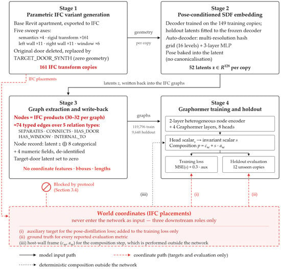
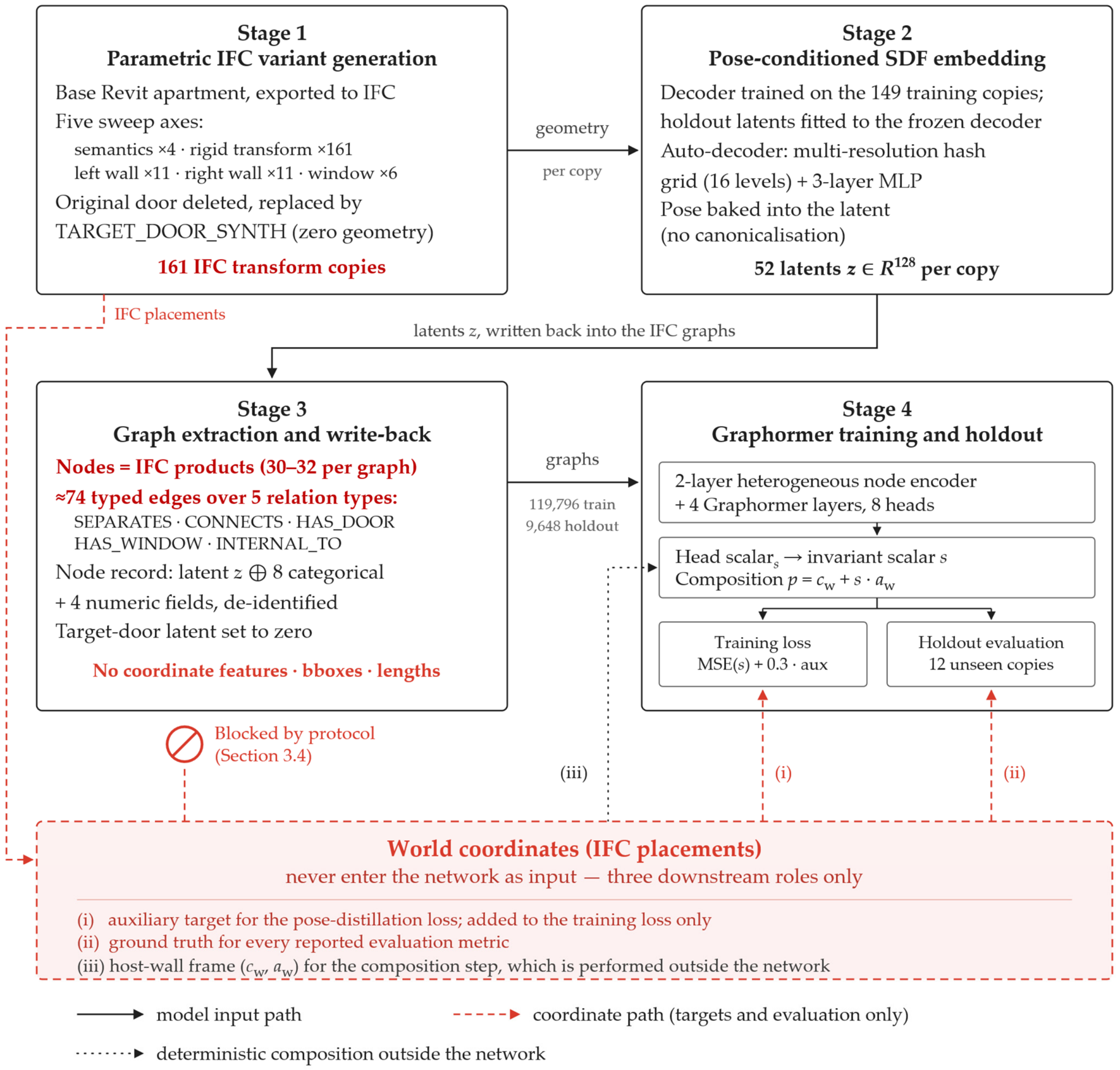
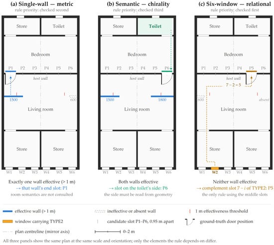
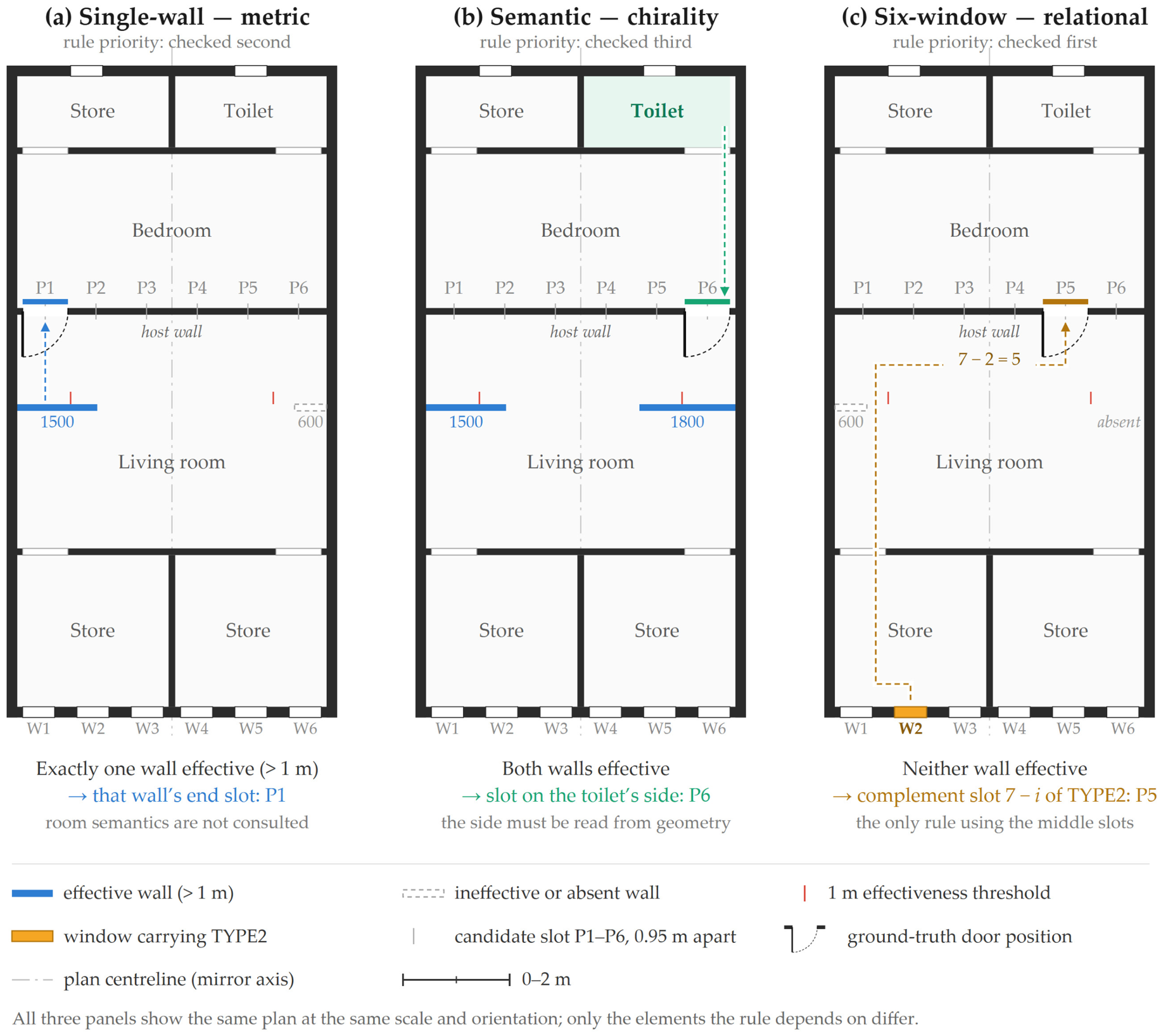
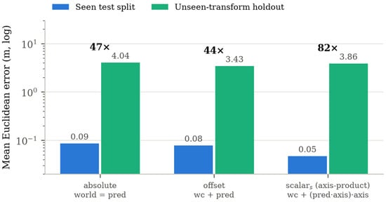
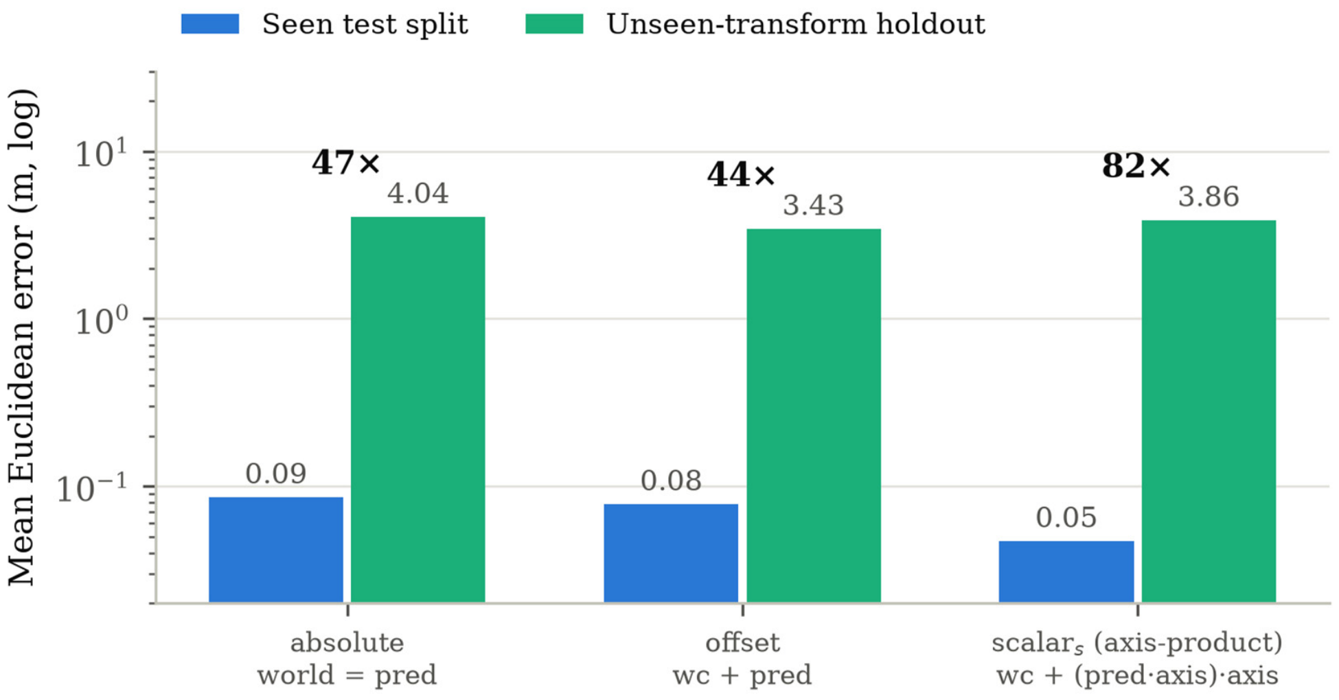
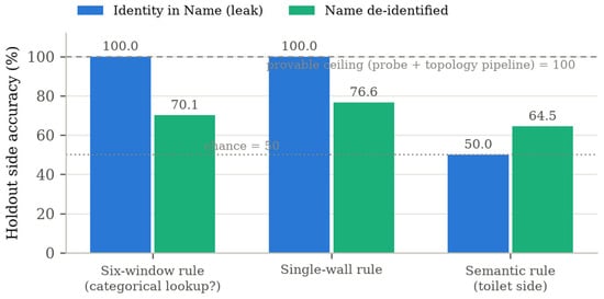
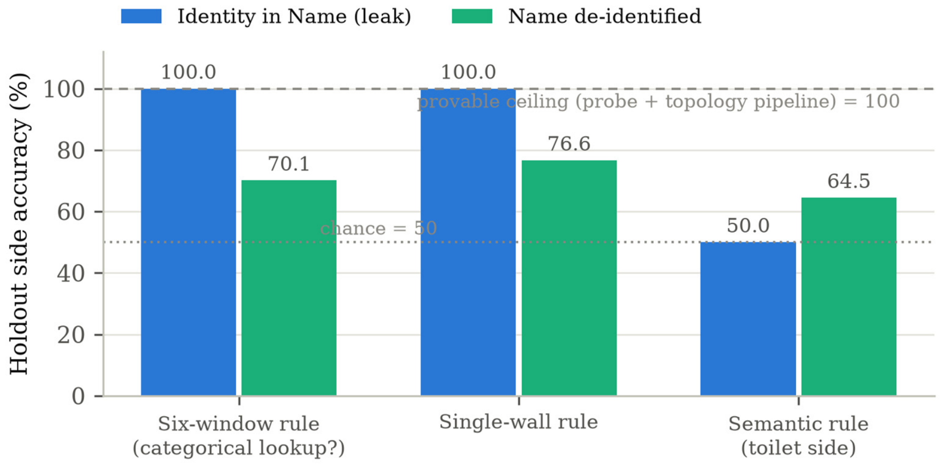
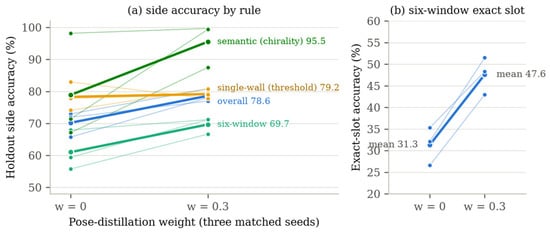
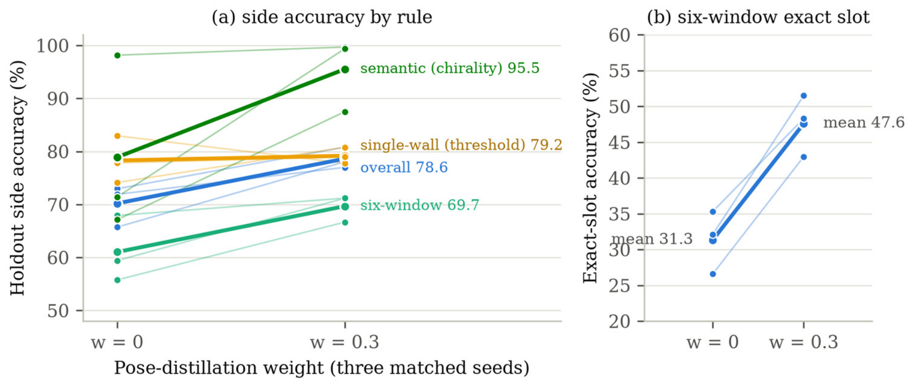
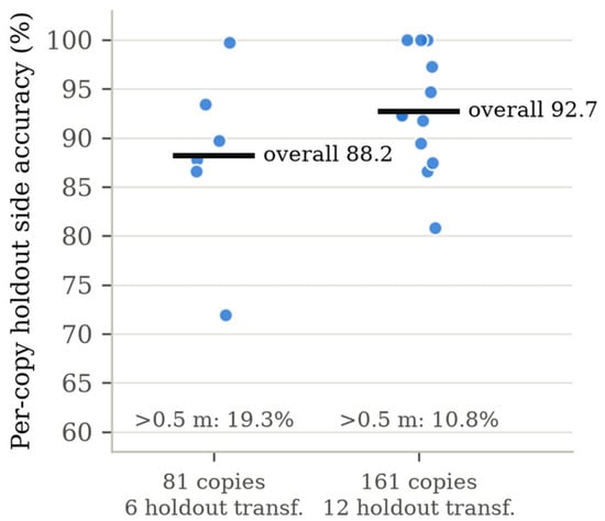
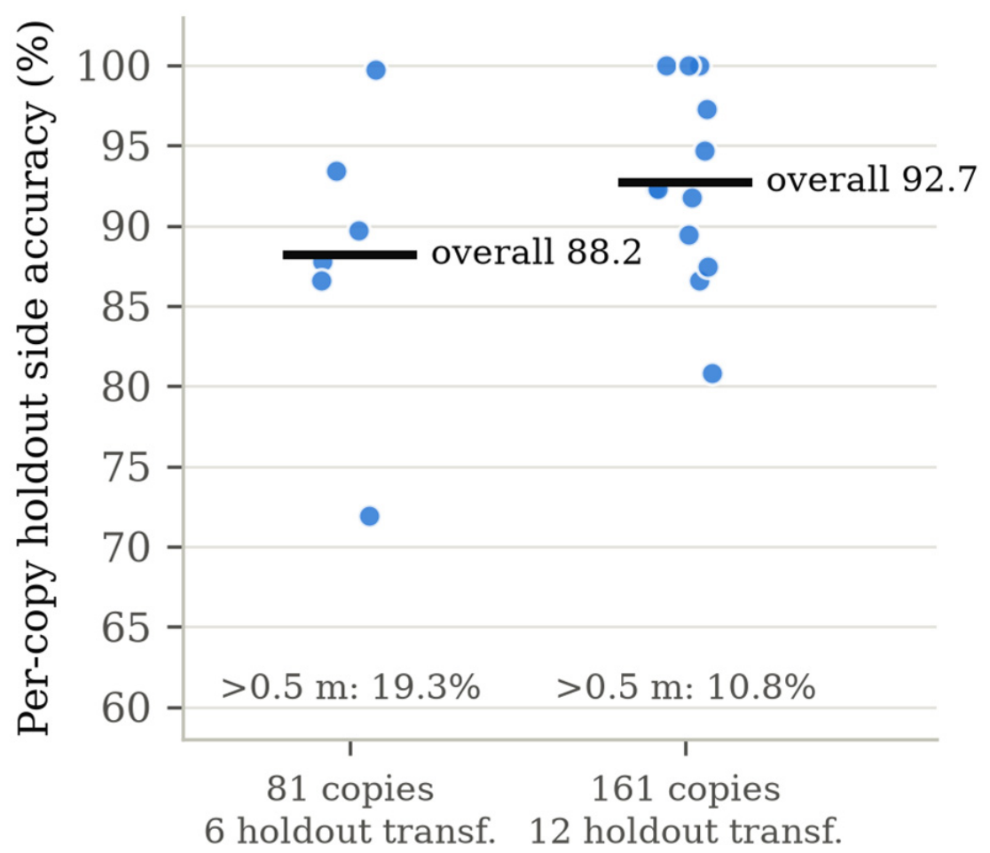
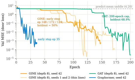
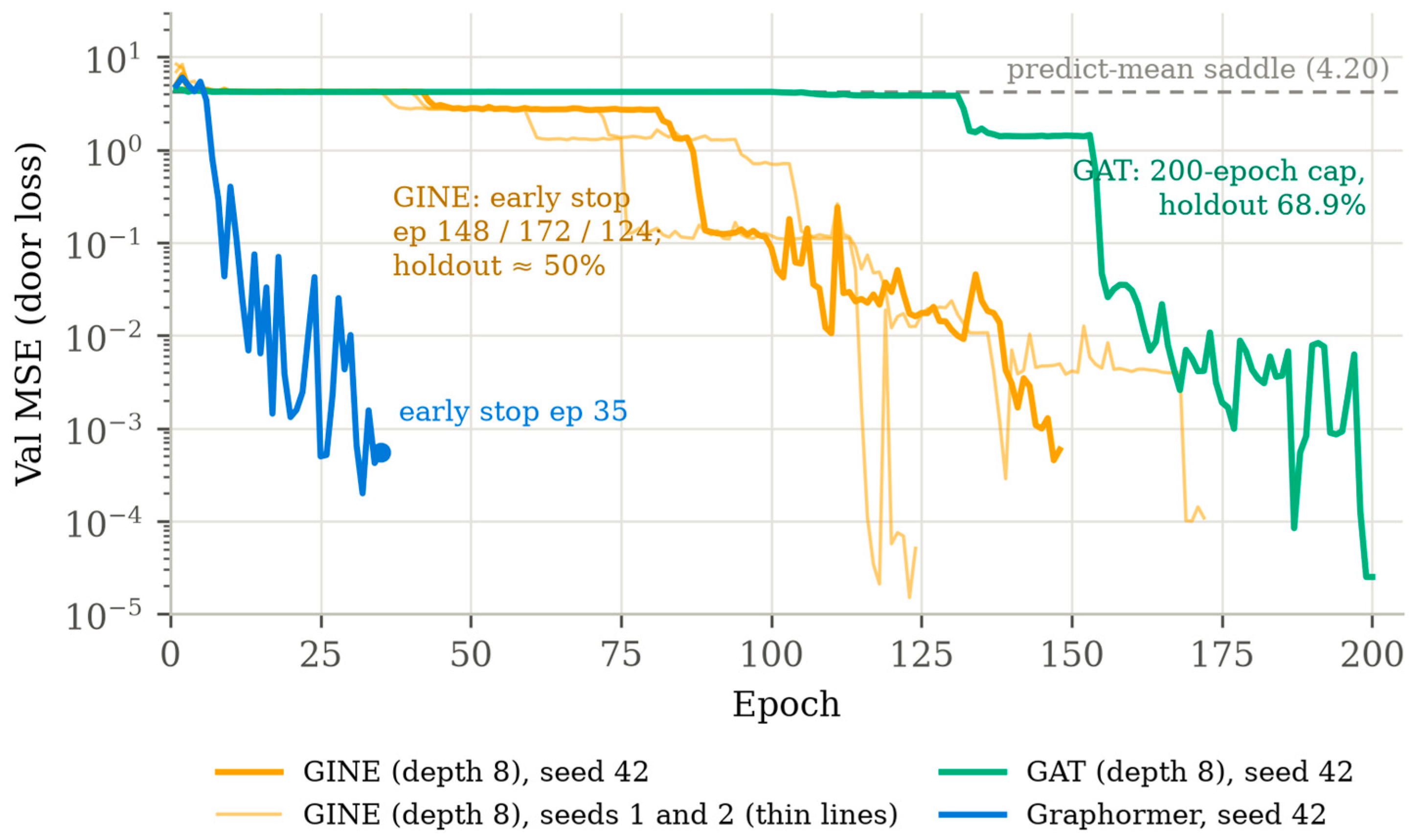
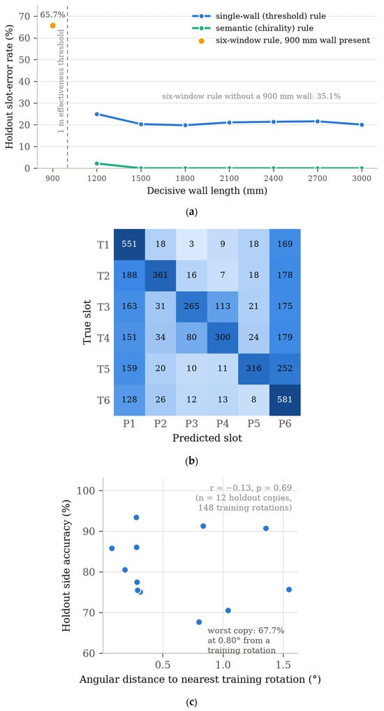
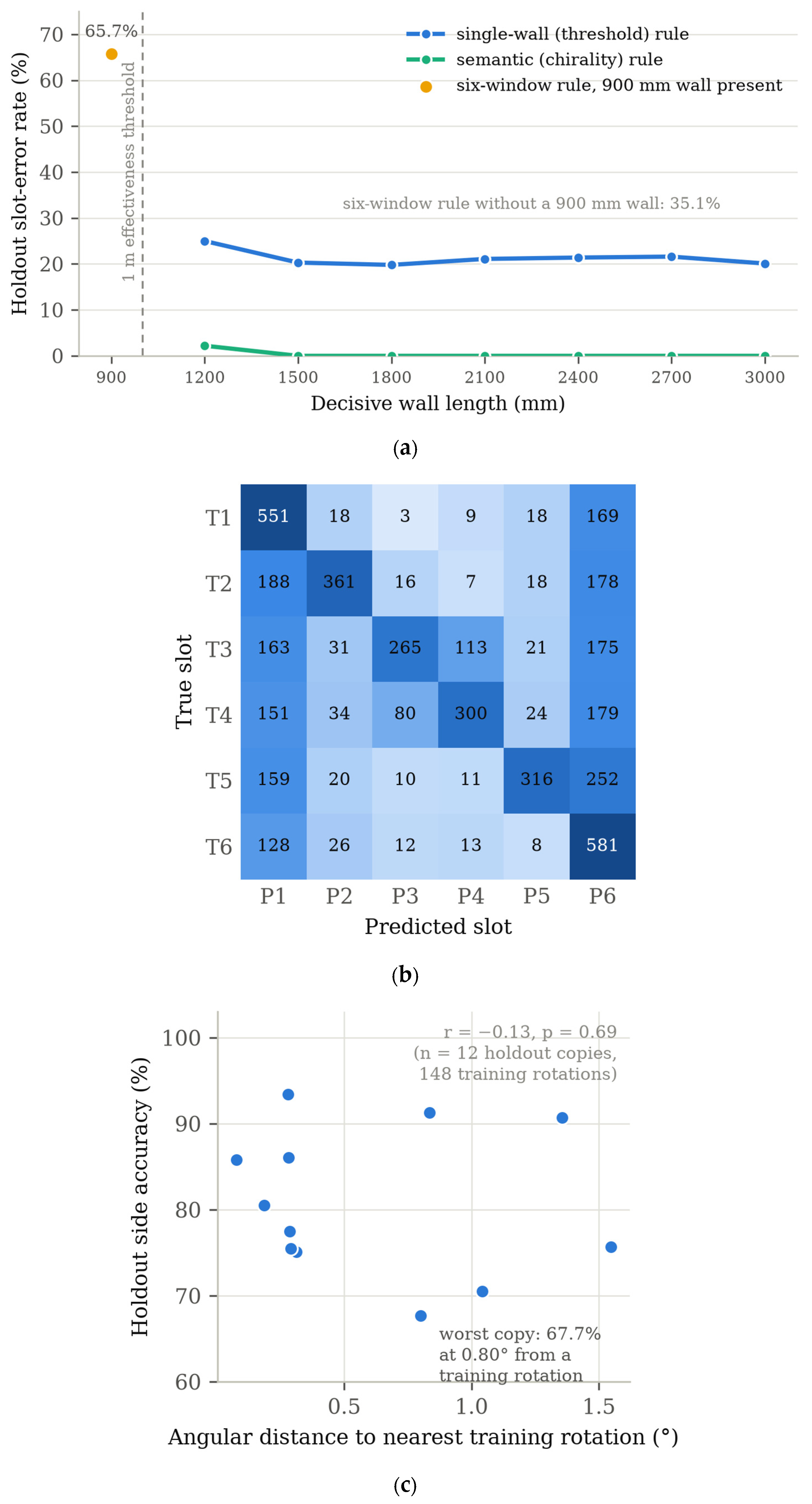
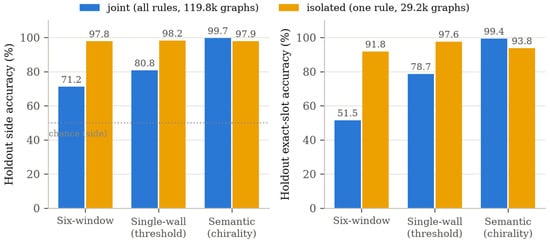
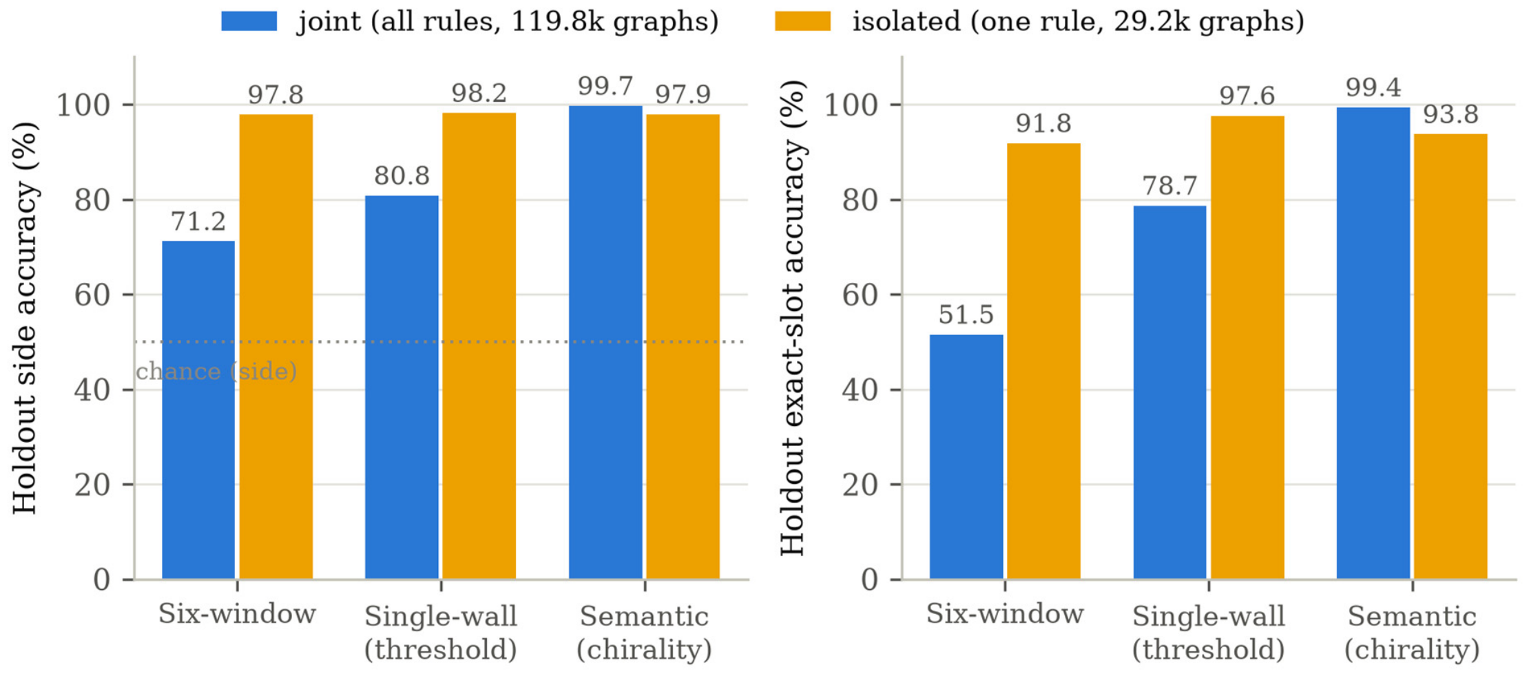
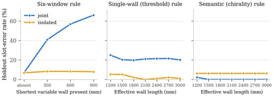
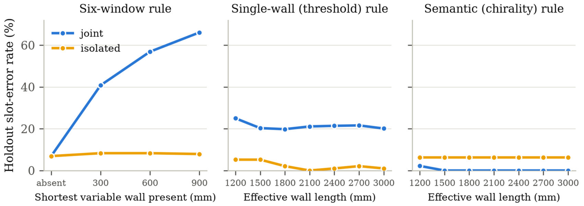
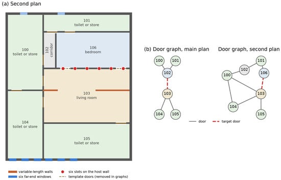
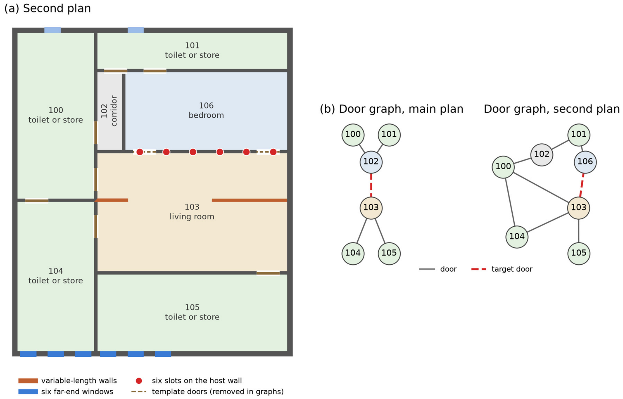

Disclaimer/Publisher’s Note: The statements, opinions and data contained in all publications are solely those of the individual author(s) and contributor(s) and not of MDPI and/or the editor(s). MDPI and/or the editor(s) disclaim responsibility for any injury to people or property resulting from any ideas, methods, instructions or products referred to in the content. |
© 2026 by the authors. Licensee MDPI, Basel, Switzerland. This article is an open access article distributed under the terms and conditions of the Creative Commons Attribution (CC BY) license.