Prediction of Anchorage Support Parameters for Underground Caverns Using Neural Networks Enhanced by Variational Information Bottleneck

Abstract

Accurate prediction of anchorage support parameters is important for the design of underground caverns. However, the limited availability of engineering cases makes it difficult to establish reliable data-driven prediction models. In this study, a neural-network-based framework was developed to predict anchorage support parameters using geological and engineering information from 121 underground cavern cases. Five input variables, including rock mass classification, excavation span, excavation height, uniaxial compressive strength, and maximum principal stress, were used to predict five support parameters. CNN and MLP models were established, and a variational information bottleneck (VIB) strategy was introduced to reduce redundant information and mitigate overfitting under small-sample conditions. The prediction performance of conventional and VIB-enhanced models was evaluated using mean relative error. The results show that the introduction of VIB improves the prediction accuracy of both CNN and MLP models, with the IB-CNN model achieving the best overall performance. An engineering application example further demonstrates the potential of the proposed method for preliminary anchorage parameter estimation. The proposed framework provides an auxiliary data-driven approach for underground cavern support design under limited data conditions.

1. Introduction

Large underground caverns are essential components of hydropower stations, pumped-storage facilities, and other underground infrastructures. With the increasing construction scale of underground engineering projects, the stability control of surrounding rock has become a critical issue during excavation and long-term operation [1]. The reinforcement system, especially the anchorage support system composed of rock bolts and cables, plays an important role in controlling deformation and maintaining the stability of surrounding rock [2]. The selection of appropriate anchorage support parameters, including bolt diameter, bolt length, bolt spacing, cable force, and cable spacing, directly affects the interaction between the support system and surrounding rock [3].

In engineering practice, the determination of anchorage support parameters is a complex process involving multiple geological and mechanical factors. Parameters such as rock mass classification, excavation geometry, rock strength, and in situ stress conditions jointly influence the selection of reinforcement schemes [4,5,6,7]. Traditional design methods mainly rely on empirical criteria, analytical calculations, numerical simulations, and engineering experience [8,9,10]. These approaches have achieved significant success in practical applications; however, they generally require detailed geological investigations, extensive parameter calibration, and considerable computational effort. Furthermore, during the preliminary design stage of large underground caverns, engineers often need to rapidly evaluate multiple potential support schemes, creating a demand for efficient prediction approaches based on existing engineering experience [11].

In recent years, machine learning (ML) methods have been increasingly applied in underground engineering due to their ability to establish nonlinear relationships between input parameters and engineering responses [12]. Previous studies have demonstrated the potential of machine learning in areas such as surrounding rock classification, tunnel deformation prediction, stability assessment, and mechanical parameter estimation.

Several investigations have reported the potential of machine learning methods in predicting complex geotechnical responses in underground engineering. Mahdevari and Torabi [13] developed artificial neural network models to predict tunnel convergence using geological and geomechanical parameters obtained from the Ghomroud water conveyance tunnel. Adoko et al. [14] investigated the prediction of tunnel convergence using artificial neural networks and multivariate adaptive regression splines based on field monitoring data from the Daguan tunnels in China. More recently, Zhang et al. [15] conducted a comparative study of hybrid metaheuristic and machine learning algorithms for predicting tunneling-induced ground settlement, highlighting the applicability of data-driven approaches to nonlinear deformation prediction.

These studies demonstrate that machine learning models can effectively establish relationships among geological conditions, engineering parameters, and underground structural responses. However, most existing applications focus on predicting tunnel convergence or ground settlement, rather than simultaneously determining multiple anchorage support parameters. Therefore, further investigation is required to evaluate the applicability of machine learning methods for the preliminary prediction of bolt diameter, bolt length, bolt spacing, cable design force, and cable spacing. In addition, the generalization capability and regularization strategies of such models require particular attention when only limited engineering data are available.

Unlike fields such as image recognition and natural language processing, which benefit from large-scale datasets, underground engineering applications are often constrained by limited data availability. Each underground cavern project requires extensive geological investigations, construction records, and monitoring information, resulting in relatively small engineering databases [16]. Under such small-sample conditions, the direct application of complex machine learning models may increase the risk of overfitting and reduce prediction reliability. Therefore, developing effective and robust prediction methods for limited engineering datasets remains a critical challenge in engineering-oriented machine learning applications [17,18,19,20].

To address the overfitting problem associated with limited datasets, appropriate regularization strategies are required to improve the generalization capability of prediction models [21,22,23,24]. The variational information bottleneck (VIB) method provides an information-theoretic regularization framework by learning compact latent representations while reducing redundant information contained in input variables [25,26,27]. By constraining unnecessary feature information and retaining task-related representations, VIB has shown potential for improving the robustness of neural networks, particularly when training data are limited [28,29,30]. Therefore, introducing the VIB mechanism into engineering prediction models may provide an effective approach for small-sample underground engineering problems [31].

Although machine learning methods have been applied to various underground engineering prediction tasks, studies focusing specifically on small-sample prediction of anchorage support parameters remain limited. In addition, previous studies often evaluate model performance using a single data partition without reporting the variance across different splits, while the reliability and generalization ability of prediction models under engineering data constraints require further investigation. A systematic framework incorporating robust cross-validation, multiple neural network baselines, and comprehensive evaluation metrics is therefore necessary for small-sample anchorage support prediction. In this study, a small-sample data-driven framework is developed for predicting anchorage support parameters of underground caverns based on a variational information bottleneck neural network. A database containing 121 engineering cases is established, where geological and mechanical parameters are used as input variables, and five key anchorage support parameters are selected as prediction targets, including bolt diameter, bolt length, bolt spacing, cable design force, and cable spacing. The main contributions of this study are summarized as follows:

(1) A small-sample underground cavern support database is established, and the relationships between geological conditions and anchorage support parameters are investigated through data-driven analysis.

(2) A variational information bottleneck (VIB) neural network framework is developed for the first time in the context of underground cavern support parameter prediction, which improves the generalization capability of neural networks under limited engineering data conditions by learning compact feature representations. Unlike previous studies that directly apply standard neural networks without addressing small-sample overfitting, this study systematically investigates the effectiveness of VIB regularization and compares it with alternative regularization strategies through ablation experiments.

(3) The proposed framework is systematically evaluated through five-fold cross-validation, comparison with multiple neural network baselines (BP, CNN, MLP), ablation experiments with alternative regularization methods (dropout, L2, deterministic bottleneck), and an engineering application demonstration to assess its applicability for anchorage support parameter prediction.

The proposed framework provides a data-driven approach for preliminary prediction of anchorage support parameters and offers a potential solution for small-sample machine learning applications in underground engineering.

2. Influencing Factors of Anchorage Support Parameters

The determination of anchorage support parameters for underground caverns is influenced by multiple geological and engineering factors. The mechanical behavior of surrounding rock, excavation geometry, and in situ stress conditions jointly affect the selection of reinforcement schemes. Therefore, identifying the key factors affecting anchorage support parameters is essential for establishing reliable prediction models.

In underground cavern engineering, the support system is designed according to the geological conditions and excavation characteristics. Among various influencing factors, rock mass quality, excavation scale, rock mechanical properties, and stress environment are considered to be the main factors controlling the design of anchorage systems.

(1) Geological factors.

① Geostress.

During the gradual excavation of an underground chamber, the original stress equilibrium of the surrounding rock will be broken. To find a new stable state, a complex stress redistribution phenomenon occurs in the surrounding rock. During this process, damage may occur in specific areas of stress concentration; this phenomenon is reflected in rock mechanics as well as in underground engineering theory. Therefore, under high-stress conditions, the contradiction between this stress concentration and the strength of the surrounding rock is particularly sharp, making the problem more complicated.

② Rock structure.

The strength, integrity, degree of joint development and weathering state of the rock body directly affect the bearing capacity and stability of the supporting structure. In weak, broken or weathered rock mass, it is necessary to use stronger support measures, such as increasing the number, diameter and length of anchor rods (ropes) or improving the stiffness and strength of the support structure at the structural surface of the constituent units of the rock mass. The effect on the integrity of the rock mass and the stability of the underground cavern enclosure is more significant.

(2) Engineering factors.

Engineering conditions mainly describe the geometric characteristics of underground caverns and their influence on stress redistribution during excavation. In this study, excavation span and excavation height are considered as important engineering factors because they directly affect the deformation behavior of surrounding rock and the requirements of reinforcement systems. The shape of the chambers has a significant impact on stress redistribution and stability, particularly at high-stress levels, and it is important that the axes of the chambers are arranged in such a way as to minimise the adverse effects of the stresses and to take into account the intermediate principal stresses. The height of the layers, the type of support and the timing of the excavation are critical to controlling the deformation of the surrounding rock. High-strength, high-prestressing anchors can be used on time to contain the deformation, but lagging support is likely to exacerbate the damage.

By analysing the stability of the surrounding rock as described above and weighing each of the influencing factors, the surrounding rock grade, excavation span, height, uniaxial saturated compressive strength of the rock, and the maximum principal stress were taken as the controlling factors in the selection of the anchoring support parameters (Table 1).

Table 1. Input and output variables of the prediction model.

Type	Variable	Symbol	Unit
Input	Rock mass classification	RMC	-
Input	Excavation span	B	m
Input	Excavation height	H	m
Input	Uniaxial compressive strength	UCS	MPa
Input	Maximum principal stress	σmax	MPa
Output	Bolt diameter	D	mm
Output	Bolt length	L	m
Output	Bolt spacing	Sb	m
Output	Cable design force	Pc	kN
Output	Cable spacing	Sc	m

Based on the analysis of geological and engineering factors, five parameters, including rock mass classification, excavation span, excavation height, uniaxial compressive strength, and maximum principal stress, were selected as input variables for the prediction model. The corresponding anchorage support parameters, including bolt diameter, bolt length, bolt spacing, cable design force, and cable spacing, were selected as prediction targets. Therefore, the prediction problem in this study can be regarded as a multi-output regression problem between geological conditions and anchorage support parameters.

3. Prediction Model for Anchorage Support Parameters

In this study, a data-driven prediction framework is developed to establish the nonlinear relationship between geological conditions and anchorage support parameters of underground caverns. It should be clarified that the variational information bottleneck (VIB) method itself is not novel; it was originally proposed by Tishby et al. (1999) [25] and extended to deep networks by Alemi et al. (2017) [26]. The contribution of this study lies in the application of VIB as a regularization strategy to the specific problem of underground cavern support parameter prediction under small-sample conditions, where engineering datasets are typically limited and overfitting is a critical concern. The proposed framework consists of two neural network backbones (CNN and MLP), each enhanced with a VIB module for feature representation optimization. The geological and engineering parameters are used as inputs, and the five anchorage support parameters are prediction targets.

3.1. CNN-Based Prediction Model with Variational Information Bottleneck

The CNN model was employed as a neural-network baseline for comparison. The five geological and engineering variables were used as model inputs, including rock mass classification, excavation span, excavation height, uniaxial compressive strength, and maximum principal stress. The model simultaneously predicted five anchorage support parameters: bolt diameter, bolt length, bolt spacing, cable design force, and cable spacing. Considering the limited size of the engineering dataset, a compact network architecture was adopted to reduce the risk of excessive model complexity. Although CNNs are commonly used for image-based tasks, this study applies CNN as a nonlinear feature extraction model for numerical engineering data. The purpose is to extract potential relationships between geological conditions and anchorage support parameters rather than perform image recognition.

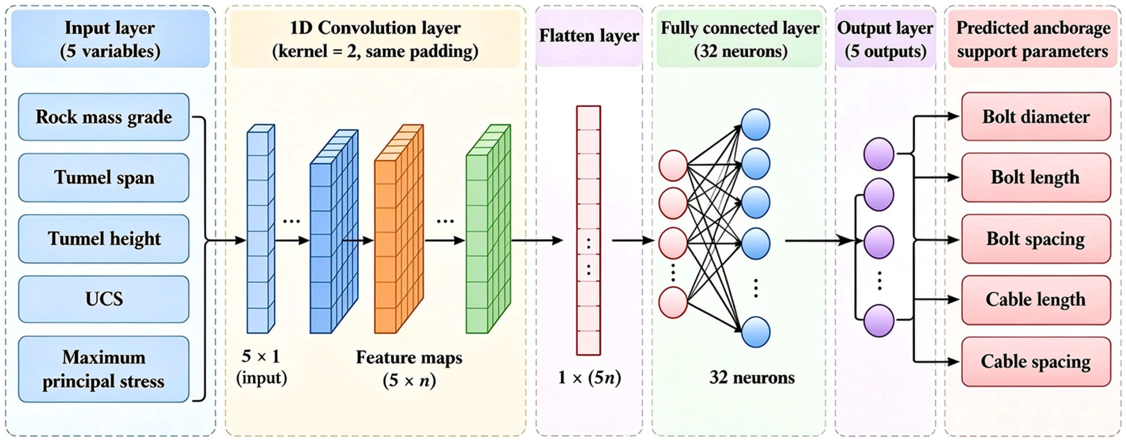
The CNN architecture used in this study is a one-dimensional (1D) convolutional network designed for numerical feature inputs. The five input variables are reshaped into a 1D feature vector of shape (5,1), ordered as rock mass classification, excavation span, excavation height, uniaxial compressive strength, and maximum principal stress. The network consists of two 1D convolutional layers: the first layer has 16 filters with a kernel size of 2, and the second layer has 32 filters with a kernel size of 2. Both layers use ReLU activation and same padding. The convolutional output is then flattened and passed through a fully connected layer with 32 neurons (ReLU activation), followed by the VIB layer with a dimension of 4. The decoder is a fully connected layer with 5 neurons and linear activation, producing the five support parameter predictions.

The five input variables were arranged in a fixed order before being fed into the one-dimensional CNN. Since these engineering variables have no inherent spatial or sequential adjacency, the convolutional features may depend on their ordering. Therefore, the CNN is used here as a data-driven feature extraction model, and its sensitivity to input ordering remains a limitation of the present study.

The information bottleneck (IB) principle, originally proposed by Tishby et al. (1999) [25], aims to find a compressed representation T of the input X that retains only information relevant to predicting the target Y. Specifically, the IB method seeks to minimize the mutual information I(X;T) between the input and the intermediate representation (compression), while simultaneously maximizing the mutual information I(T;Y) between the representation and the prediction target (relevance). In this study, the VIB is applied to the CNN model by inserting a stochastic bottleneck layer that compresses the input geological and engineering information and preserves only the features useful for predicting the anchorage support parameters. Figure 1 shows the schematic diagram of the VIB-enhanced CNN.

Figure 1. Information bottleneck improvement convolutional neural network schematic diagram.

The following is the derivation of the formulae for introducing the information bottleneck into the conventional neural network.

In the IB framework, the optimal intermediate representation T is found by minimizing the IB Lagrangian, which compresses the input information I(X;T) while retaining information relevant to the prediction target I(T;Y), as expressed in Equation (1):

$$\min {\mathcal{L}}_{\mathrm{IB}}=-\mathrm{I}\left(\mathrm{T};\mathrm{Y}\right)+\mathsf{\beta }\mathrm{I}\left(\mathrm{X};\mathrm{T}\right)$$

(1)

In this framework, I(X;T) represents the information transferred from input variables to the intermediate representation, while I(T;Y) represents the information related to prediction targets. Therefore, the optimization process attempts to remove redundant input information and retain task-related features.

The intermediate representation is generated through the bottleneck layer, which provides a compressed feature space for subsequent prediction.

The objective of this optimization is to find the optimal intermediate representation T that retains sufficient information about the output Y while minimizing redundant information from the input X. This compression–relevance trade-off enhances the generalization ability of the model and reduces overfitting, thereby improving prediction performance on small engineering datasets.

In this study, the final optimization objective of the VIB-CNN model combines prediction loss and KL divergence regularization.

Combining the above, the final optimisation objective function can be expressed as Equation (2):

$${\mathcal{L}}_{\mathrm{VIB}}={\mathcal{L}}_{\mathrm{pred}} + {\mathsf{\beta }\mathrm{D}}_{\mathrm{KL}}\left({\mathrm{q}}_{\mathsf{\varphi }}(\mathrm{T}|\mathrm{X})\Vert \mathrm{p}\left(\mathrm{T}\right)\right)$$

(2)

Here, β controls the trade-off between prediction accuracy and information compression. The same definition of β is used throughout the theoretical formulation and model training. The prediction loss ensures the accuracy of anchorage parameter prediction, while the KL divergence term constrains the latent representation and reduces redundant information.

Implementation details of the variational information bottleneck. In this study, the VIB is implemented as follows. The encoder q(T|X) is parameterized as a Gaussian distribution with a learned mean and standard deviation:

$${\mathrm{q}\left(\mathrm{T}\right|\mathrm{X}) = \mathrm{N}(\mathsf{\mu }}_{\mathsf{\varphi }}\left(\mathrm{X}\right),{\mathsf{\sigma }}_{\mathsf{\varphi }}^2\left(\mathrm{X}\right)\mathrm{I})$$

(3)

where $\varphi$ denotes the encoder network parameters, and ${\mu }_{\varphi }\left(X\right)$ and ${\sigma }_{\varphi }\left(X\right)$ represent the mean and standard deviation of the Gaussian encoder distribution, respectively. The prior distribution $p\left(\mathrm{T}\right)$ is set to the standard multivariate normal distribution N(0, I). The reparameterization trick is used during training: a latent sample is generated as Equation (4):

$$\mathrm{T} = \mathsf{\mu } + \mathsf{\sigma } \cdot \mathsf{\epsilon }$$

(4)

where ε ~ N(0, I), enabling gradient backpropagation through the stochastic sampling. The decoder p(Y|T) is parameterized as a Gaussian distribution with a learned mean and fixed unit variance, which is equivalent to minimizing the mean squared error (MSE) loss between the predicted and true support parameters. At test time, the mean of the latent distribution ${\mu }_{\varphi }\left(X\right)$ is used as the deterministic representation (i.e., no random sampling), ensuring reproducible predictions. The bottleneck dimension is set to 4, and the trade-off coefficient β is set to 0.01.

3.2. Improved Multilayer Perceptron Neural Network Model Derivation

A multilayer perceptron (MLP) is a fully connected feed-forward neural network capable of approximating nonlinear relationships between input and output variables. In this study, the MLP model uses five geological and engineering parameters as inputs, including rock mass classification, excavation span, excavation height, uniaxial compressive strength, and maximum principal stress. The model simultaneously predicts five anchorage support parameters, including bolt diameter, bolt length, bolt spacing, cable design force, and cable spacing.

(1) Basic structure of MLP.

The engineering geological parameters are represented by $X\in {ℝ}^{n\times 5}$, where n is the number of samples. The anchorage support parameters are represented by $Y\in {ℝ}^{n\times d}$ The hidden layer representation of a standard MLP is $H$, and the output is represented as $\widehat{Y}$, as expressed in Equations (5) and (6).

$$\mathrm{h}=\mathsf{\sigma }\left({\mathrm{W}}_1\mathrm{X}+{\mathrm{b}}_1\right)$$

(5)

$$\hat{\mathrm{y}}={\mathrm{W}}_2\mathrm{h}+{\mathrm{b}}_2$$

(6)

where ${\mathrm{W}}_1$ and ${\mathrm{W}}_2$ are the weight matrices of the hidden and output layers, respectively; ${\mathrm{b}}_1$ and ${\mathrm{b}}_2$ are the corresponding bias vectors; h represents the hidden-layer representation; and $\mathsf{\sigma }\left(·\right)$ denotes the ReLU activation function. Because five support parameters are predicted simultaneously, the output layer contains five neurons. The ReLU activation function is applied to the hidden layer, while the output layer uses a linear transformation to predict the five continuous anchorage support parameters. The 121 engineering cases were used to establish the nonlinear relationship between the five input variables and the five anchorage support parameters.

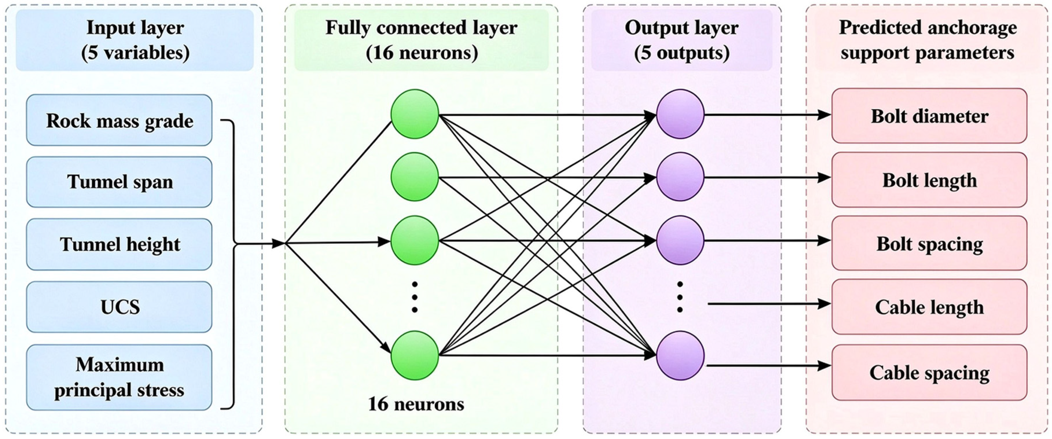
CNN and MLP are different neural-network architectures with different feature-extraction mechanisms. However, the information bottleneck can be introduced into the intermediate representation of both models using the same regularization principle. Therefore, the IB formulation described in Section 3.1 is not repeated here. For the MLP model, the information bottleneck layer is introduced between the hidden representation and the subsequent prediction layers to constrain redundant information while preserving features relevant to the prediction of anchorage support parameters. The resulting architecture is referred to as the IB + MLP model, as illustrated in Figure 2.

Figure 2. Architecture of the Variational Information Bottleneck-Enhanced Multilayer Perceptron (VIB-MLP).

To ensure a consistent comparison, the conventional MLP and IB + MLP models used the same input and output variables and the same data-processing procedure. The hidden layers used ReLU activation. The information bottleneck was introduced only in the IB + MLP model, while the conventional MLP was used as the baseline model.

The hidden-layer size was set to 16 neurons, the bottleneck dimension was set to 4, and the information-bottleneck coefficient β was set to 0.01. A compact network architecture was adopted considering the limited dataset size to reduce excessive model complexity and mitigate overfitting.

3.3. Mechanism of Information Bottleneck Regularization

The information bottleneck is introduced as a regularization mechanism to reduce redundant information in the intermediate feature representation while preserving information relevant to anchorage support prediction. Rather than directly estimating mutual information, the proposed models employ a variational objective combining prediction loss with KL-divergence regularization. The KL-divergence term constrains the learned latent distribution toward a predefined prior, while the prediction loss maintains its relevance to the five target support parameters.

The coefficient β controls the balance between these two objectives. For the relatively small engineering dataset considered in this study, this constraint is expected to mitigate overfitting, although its effectiveness must be established empirically. Section 4 evaluates this effect by comparing the prediction performance of the conventional CNN and MLP models with their information bottleneck-enhanced counterparts, IB-CNN and IB-MLP.

3.4. Model Evaluation Indicators

The predictive performance of the models was evaluated by comparing the predicted anchorage support parameters with the corresponding observed engineering values. Because the five output variables have different physical units and numerical ranges, the prediction error was expressed using relative error rather than the direct difference between predicted and observed values. The relative error for each prediction is defined as the absolute difference between the predicted value and the observed value divided by the observed value.

$${\mathit{RE}}_{\mathit{i}}={\displaystyle \frac{\left|{\hat{\mathit{y}}}_{\mathit{i}}{-\mathit{y}}_{\mathit{i}}\right|}{{\mathit{y}}_{\mathit{i}}}}$$

(7)

where ${\mathit{RE}}_{\mathrm{i}}$ = relative error of the i-th sample; ${\hat{\mathit{y}}}_{\mathit{i}}$ = predicted value of the i-th sample; ${\mathit{y}}_{\mathit{i}}$ = observed value of the i-th sample.

To ensure the mathematical consistency of the evaluation metrics, MAE, RMSE, and R² were defined using the same set of reference values and out-of-fold predictions. Under the five-fold cross-validation framework, each of the 121 engineering cases contributes one out-of-fold prediction for each target parameter and prediction model.

For each prediction target, MAE and RMSE quantify the absolute magnitude of prediction errors, whereas R² measures the proportion of variance explained relative to the mean of the reference values. The three metrics must be calculated from the same prediction records to ensure that their numerical values are mutually consistent.

The mean absolute error (MAE) is calculated as Equation (8):

$$\mathit{MAE} = {\displaystyle \frac{1}{\mathit{n}}}{{\displaystyle \mathit{\sum }}}_{\mathit{i}=1}^{\mathit{n}}\left|{\hat{\mathit{y}}}_{\mathit{i}}{-\mathit{y}}_{\mathit{i}}\right|$$

(8)

The root mean square error (RMSE) is expressed as Equation (9):

$$\mathit{RMSE} = \sqrt{{\displaystyle \frac{1}{\mathit{n}}}{{\displaystyle \mathit{\sum }}}_{\mathit{i}=1}^{\mathit{n}}{\left({\hat{\mathit{y}}}_{\mathit{i}}{-\mathit{y}}_{\mathit{i}}\right)}^2}$$

(9)

The coefficient of determination $R^2$ is defined as Equation (10):

$${\mathit{R}}^2 = 1-{\displaystyle \frac{{{\displaystyle \sum }}_{\mathit{i}=1}^{\mathit{n}}{\left({\hat{\mathit{y}}}_{\mathrm{i}}{-\mathit{y}}_{\mathit{i}}\right)}^2}{{{\displaystyle \sum }}_{\mathit{i}=1}^{\mathit{n}}{\left(\stackrel{-}{\mathit{y}}{-\mathit{y}}_{\mathit{i}}\right)}^2}}$$

(10)

where n = total number of prediction samples and $\stackrel{-}{\mathit{y}} = {\displaystyle \frac{1}{\mathit{n}}}{{\displaystyle \sum }}_{\mathit{i}=1}^{\mathit{n}}{\mathit{y}}_{\mathit{i}}=$ mean value of observed samples.

4. Results and Analysis of Model Performance

This section evaluates the prediction performance of five neural network models using 121 underground cavern engineering cases. The evaluation procedure, including data partitioning and preprocessing, is described in Section 4.1. The subsequent sections present the comparative prediction results and engineering application analysis.

4.1. Dataset Partition and Model Comparison Settings

The dataset comprises 121 engineering cases, each containing five geological and engineering input variables and five anchorage support parameters. Model performance was evaluated using five-fold cross-validation. The cases were divided into five non-overlapping folds, each containing 24 or 25 cases. In each iteration, four folds were used for model development, and the remaining fold was held out for testing. Within the model-development data, 15% of the cases were reserved for validation and early stopping. The same fold partitions were used for all five models, and performance metrics were summarized across the five test folds.

Before model training, the continuous input and output variables were normalized using the statistical parameters calculated from the training set. The same normalization parameters were subsequently applied to the validation and test sets to avoid information leakage. Rock mass classification was treated as an ordinal engineering variable, with Classes II, III, and IV represented by the ordered numerical values 2, 3, and 4, respectively. The predicted values were transformed back to their original physical units before calculating the prediction errors.

Five neural-network models were considered in the comparative analysis: BP, CNN, MLP, IB + CNN, and IB + MLP. The BP, CNN, and MLP models were trained directly using the same engineering dataset rather than adopting prediction results from previous studies. The information-bottleneck-enhanced models used the same basic training data and evaluation procedure as their corresponding baseline networks. Therefore, differences in prediction performance can be mainly attributed to the introduction of the information bottleneck regularization rather than differences in data partitioning.

Among the three conventional models, the BP and MLP models differ in network width and activation function. The BP model is a single-hidden-layer feedforward network with 8 hidden neurons and sigmoid activation, representing a conventional shallow network configuration. The MLP model is also a single-hidden-layer feedforward network but with 16 hidden neurons and ReLU activation, providing a wider hidden representation and faster gradient propagation. Both models are trained using the Adam optimizer, and the only architectural differences are the hidden layer size and activation function. The CNN model uses the 1D convolutional architecture described in Section 3.1.

To maintain consistency between different models, all neural networks were trained using the Adam optimizer with an initial learning rate of 0.001 and a batch size of 16. The maximum number of training epochs was set to 500. Early stopping was applied when the validation loss did not decrease for 50 consecutive epochs. The BP model used 8 hidden neurons with sigmoid activation, while the MLP model used 16 hidden neurons with ReLU activation. For the information-bottleneck-enhanced models, the bottleneck dimension was set to 4 and the information-bottleneck coefficient β was set to 0.01, as determined by the parameter sensitivity analysis in Section 4.2.2. The same five-fold cross-validation partitions were used for all model comparisons to ensure a fair comparison.

The ten representative test cases cover a relatively broad range of geological and engineering conditions. The excavation span ranges from 16.5 to 31.9 m, while the excavation height varies from 47.0 to 87.5 m. The uniaxial compressive strength ranges from 60 to 140 MPa, and the maximum principal stress ranges from 5.0 to 29.0 MPa. The cases also include rock mass Classes II–IV. Correspondingly, the observed anchorage support schemes exhibit clear variations, including bolt diameters of 28–32 mm, bolt lengths of 6–9 m, cable design forces of 1000–2500 kN, and cable spacings of 3.0–6.0 m. These variations provide representative engineering cases for comparing the prediction behavior of different models.

To illustrate the geological conditions and anchorage support characteristics of the engineering dataset, ten representative cases are presented in Table 2 and Table 3. Table 2 summarizes the five input variables, while Table 3 provides the corresponding reference anchorage support parameters.

Table 2. Geological and engineering parameters of ten representative test cases.

Project Number	Surrounding-Rock Grade	Excavation Span/m	Excavation Height/m	Uniaxial Saturated Compressive Strength/MPa	Maximum Principal In Situ Stress/MPa
1	4	28.3	63	97.3	29
2	4	30.8	73.2	60	22.2
3	4	30	70.1	120	27.3
4	3	30.6	79.4	140	25.4
5	3	31.9	74.7	120	18
6	4	31	87.5	100	8.9
7	3	30	75.5	100	12.8
8	3	26.9	57.5	85	6.97
9	2	26.2	61.4	100	5
10	3	16.5	47	90	7.4

Table 3. Observed anchorage support parameters of ten representative test cases.

Project Number	Bolt Diameter/mm	Bolt Length/m	Bolt Spacing/m	Cable Design Force/kN	Cable Spacing/m
1	32	7	1.5	2000	4.5
2	30	7	1.5	2000	4.5
3	32	9	1.2	1800	4.5
4	30	7	1.2	1800	4.5
5	30	9	1.5	2000	3
6	28	6	1.5	2000	4.5
7	32	9	1.5	1000	5
8	30	6	1.5	1000	6
9	32	9	1.5	2500	4.5
10	30	7	1.5	2000	4.5

These ten cases are presented for descriptive and visualization purposes only. They do not constitute a separate independent test set, nor are they used as the sole basis for calculating model performance. The cross-validation evaluation is defined over all 121 engineering cases, with each case assigned to one held-out evaluation fold.

4.2. Prediction Performance Comparison of Different Neural Network Models

The predictive performance of the five neural network models was evaluated using the five-fold cross-validation framework described in Section 4.1. In each iteration, predictions were generated for the held-out evaluation fold, and the corresponding errors were calculated against the reference anchorage support parameters.

To interpret the prediction errors from an engineering perspective, the continuous prediction accuracy and the selection of discrete support specifications were considered separately. Relative error was used to quantify the deviation between predicted and reference values, whereas standard-value matching was used to assess whether a continuous prediction corresponded to the same discrete specification as the reference design. For this purpose, the candidate bolt diameters were 25, 28, 30, and 32 mm, and the candidate cable design forces were 1000, 1500, 1800, 2000, and 2500 kN, consistent with the specification sets examined in the subsequent analysis. Predictions were mapped to the nearest candidate value, and the resulting selections were compared with the corresponding reference specifications. These candidate sets are used for the present comparative analysis and should not be interpreted as universally applicable design standards. The engineering suitability of a predicted support scheme requires additional assessment against project-specific design requirements and safety constraints.

4.2.1. Prediction Results of Conventional Neural Network Models

The prediction performance of the three conventional neural network models (BP, CNN, and MLP) was evaluated using the same five-fold cross-validation procedure described in Section 4.1. Table 4 presents the predicted bolt diameters for ten representative engineering cases to facilitate qualitative comparison, while Table 5 summarizes the mean relative errors of all five models across the five anchorage support parameters.

Table 4. Predicted bolt diameter for ten representative test cases.

Case	Real	BP	CNN	MLP	IB-CNN	IB-MLP
1	32	30	30.8	30.7	31.6	31.5
2	30	27.8	31	31	30.4	30.2
3	32	29.8	31	30.9	31.6	31.6
4	30	32	30.9	30.9	30.9	30.4
5	30	28	29.2	29.1	29.7	29.6
6	28	27	29	29	28.4	28.4
7	32	30.5	31.2	31.1	31.7	31.6
8	30	27.9	29.1	29	30.3	30.3
9	32	29.7	31.1	31	31.7	31.7
10	30	32.2	31	31	30.4	30.4

The predictive performance of the five neural network models was compared using the mean relative error (MRE) for five anchorage support parameters: bolt diameter, bolt length, bolt spacing, cable design force, and cable spacing. Table 5 summarizes the five-fold cross-validation results, expressed as the mean ± standard deviation of the fold-specific MRE values. The Average column represents the arithmetic mean of the five target-specific mean errors, while its standard deviation represents the variation in the overall MRE across the five folds.

The same evaluation framework was specified for all models to facilitate comparisons between the conventional neural networks and their information-bottleneck-enhanced counterparts.

For the qualitative comparison, ten representative engineering cases were selected from the 121-case dataset. The predictions reported in Table 4 were obtained from the corresponding held-out folds during five-fold cross-validation. For each case, the reported prediction was generated by a model that had not been trained on that case. The same fold assignments were used for all five models to ensure comparability. These ten cases are presented for visualization only, whereas the quantitative performance metrics were calculated using the complete set of 121 out-of-fold predictions.

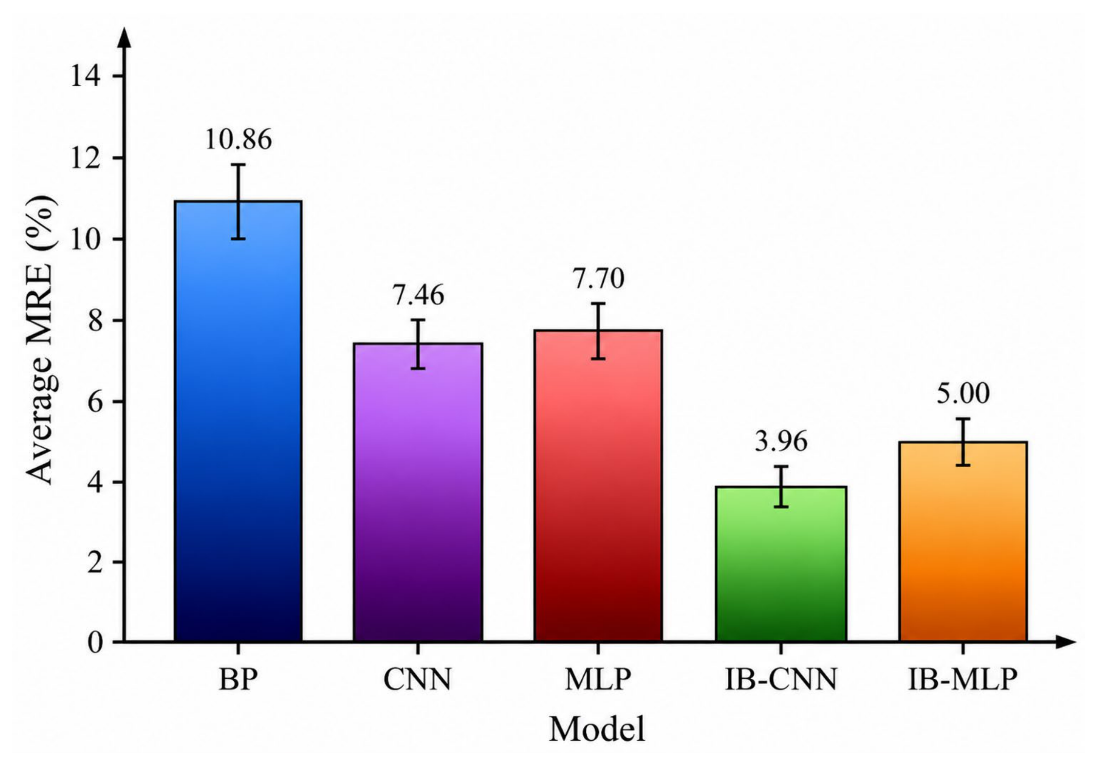
Table 5 summarizes the five-fold cross-validation results for the five models. IB-CNN achieved the lowest average MRE (3.96 ± 0.35%), followed by IB-MLP (5.00 ± 0.44%). Both models outperformed their conventional counterparts, CNN (7.46%) and MLP (7.70%), respectively. BP exhibited the highest average MRE (10.86 ± 0.88%). These results indicate that information bottleneck regularization improved prediction accuracy under the evaluated cross-validation settings.

Table 5. Mean relative error of different models based on five-fold cross-validation (Unit: %).

Model	Bolt Diameter	Bolt Length	Bolt Spacing	Cable Force	Cable Spacing	Average
BP	7.12 ± 0.83	12.68 ± 1.31	10.45 ± 1.08	14.82 ± 1.52	9.23 ± 1.14	10.86 ± 0.88
CNN	3.42 ± 0.46	9.56 ± 0.94	6.71 ± 0.65	12.03 ± 1.21	5.58 ± 0.57	7.46 ± 0.47
MLP	3.71 ± 0.51	9.84 ± 1.03	6.94 ± 0.73	12.56 ± 1.34	5.45 ± 0.62	7.70 ± 0.43
IB-CNN	1.58 ± 0.25	5.82 ± 0.56	3.74 ± 0.39	5.91 ± 0.67	2.75 ± 0.31	3.96 ± 0.35
IB-MLP	1.83 ± 0.28	6.13 ± 0.64	4.02 ± 0.43	8.67 ± 0.85	4.35 ± 0.48	5.00 ± 0.44

Table 5. Mean relative error of different models based on five-fold cross-validation (Unit: %).

Model	Bolt Diameter	Bolt Length	Bolt Spacing	Cable Force	Cable Spacing	Average
BP	7.12 ± 0.83	12.68 ± 1.31	10.45 ± 1.08	14.82 ± 1.52	9.23 ± 1.14	10.86 ± 0.88
CNN	3.42 ± 0.46	9.56 ± 0.94	6.71 ± 0.65	12.03 ± 1.21	5.58 ± 0.57	7.46 ± 0.47
MLP	3.71 ± 0.51	9.84 ± 1.03	6.94 ± 0.73	12.56 ± 1.34	5.45 ± 0.62	7.70 ± 0.43
IB-CNN	1.58 ± 0.25	5.82 ± 0.56	3.74 ± 0.39	5.91 ± 0.67	2.75 ± 0.31	3.96 ± 0.35
IB-MLP	1.83 ± 0.28	6.13 ± 0.64	4.02 ± 0.43	8.67 ± 0.85	4.35 ± 0.48	5.00 ± 0.44

Table 6 presents the comprehensive evaluation metrics for the five prediction models. To maintain consistency with the five-fold cross-validation framework, the evaluation metrics are defined using the pooled out-of-fold predictions of all 121 engineering cases.

Table 6. Comprehensive evaluation metrics of different models based on pooled out-of-fold predictions (121 cases).

Model	Metric	Bolt Diameter (mm)	Bolt Length (m)	Bolt Spacing (m)	Cable Force (kN)	Cable Spacing (m)
BP	MAE	2.10	0.89	0.16	265	0.43
	RMSE	2.62	1.13	0.20	338	0.55
	R2	−0.11	0.48	0.18	0.43	0.52
CNN	MAE	1.02	0.67	0.10	218	0.26
	RMSE	1.31	0.86	0.13	282	0.34
	R2	0.72	0.70	0.65	0.60	0.82
MLP	MAE	1.10	0.69	0.10	225	0.29
	RMSE	1.42	0.89	0.14	291	0.38
	R2	0.67	0.68	0.60	0.58	0.77
IB-CNN	MAE	0.47	0.41	0.06	108	0.13
	RMSE	0.61	0.53	0.08	143	0.18
	R2	0.94	0.89	0.87	0.90	0.95
IB-MLP	MAE	0.53	0.44	0.07	168	0.20
	RMSE	0.69	0.58	0.09	218	0.26
	R2	0.92	0.86	0.83	0.76	0.89

For each prediction target, the reference values are identical across the five models, while the predicted values differ according to the corresponding model. Consequently, the total sum of squares (SST) remains constant across models for a given target parameter. The reported RMSE and R² values must therefore satisfy their mathematical relationship under the same evaluation dataset.

The comprehensive evaluation of the prediction models considers three complementary performance metrics: MAE, RMSE, and R². Lower MAE and RMSE values indicate smaller prediction errors, while higher R² values indicate better agreement between predicted and reference values relative to a mean-value baseline.

The model comparisons should be interpreted using metrics calculated from the same pooled out-of-fold prediction records. This procedure avoids discrepancies caused by mixing evaluation subsets or combining metrics obtained from different training and testing configurations.

The relative performance of the five models should also be compared with the MRE results reported in Table 5. However, because MRE, MAE, RMSE, and R² quantify different aspects of prediction error, an identical model ranking across all metrics is not mathematically required.

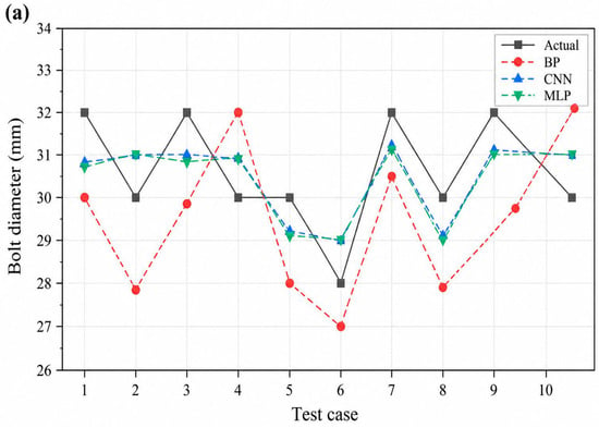
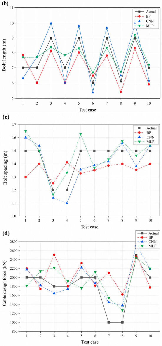
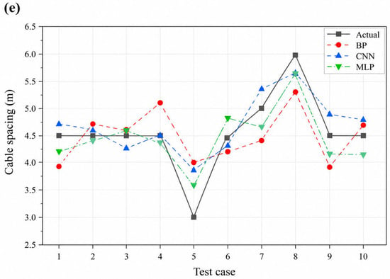
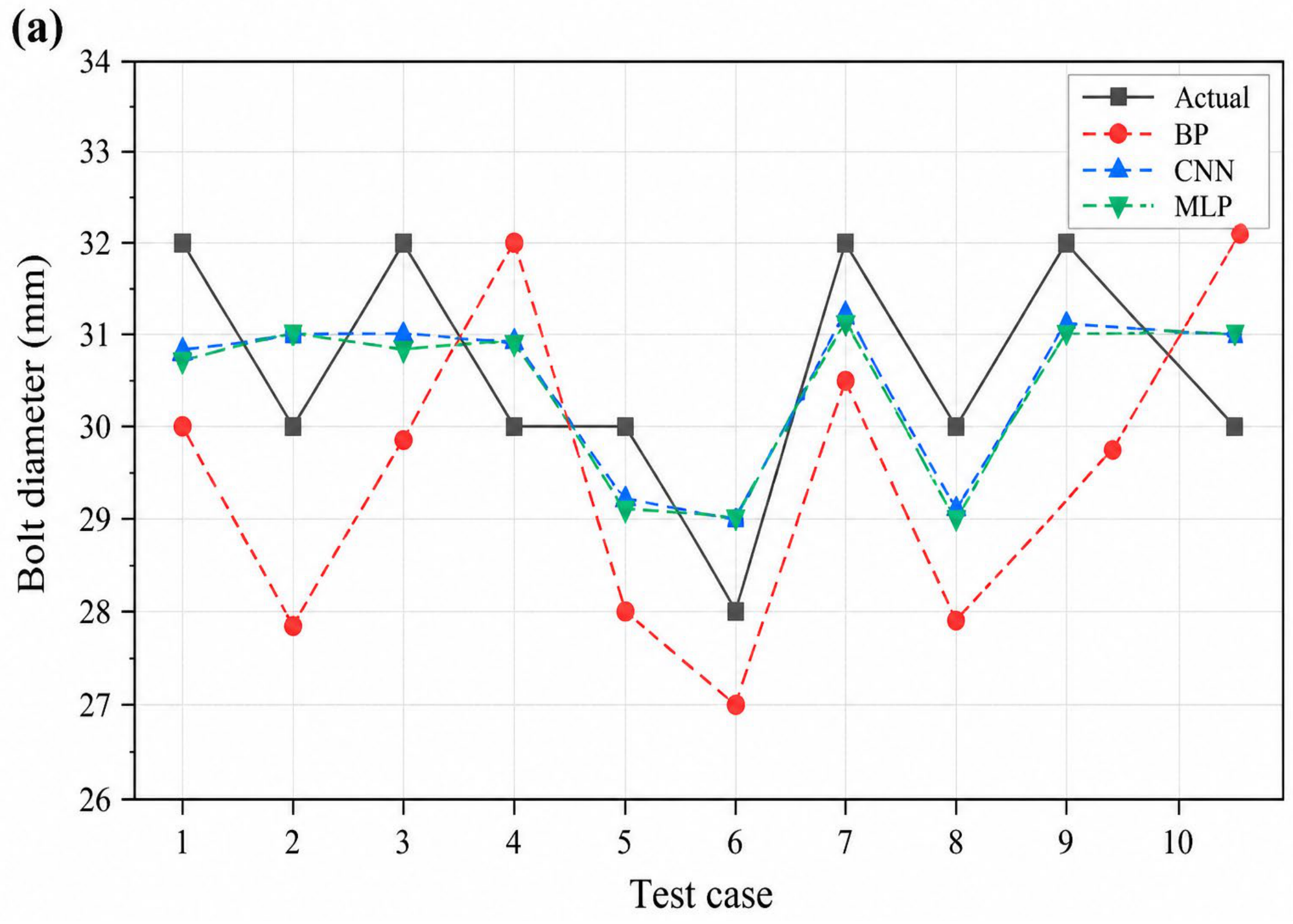
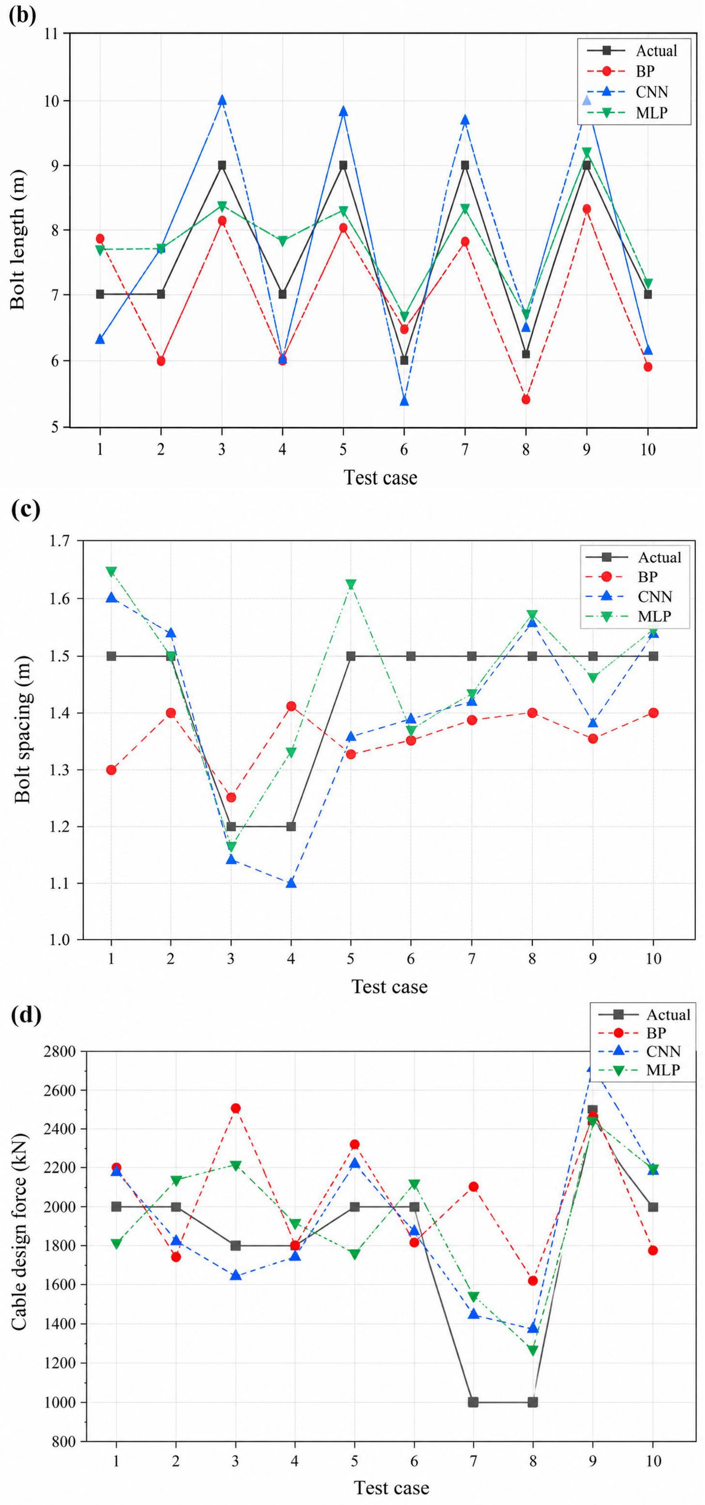
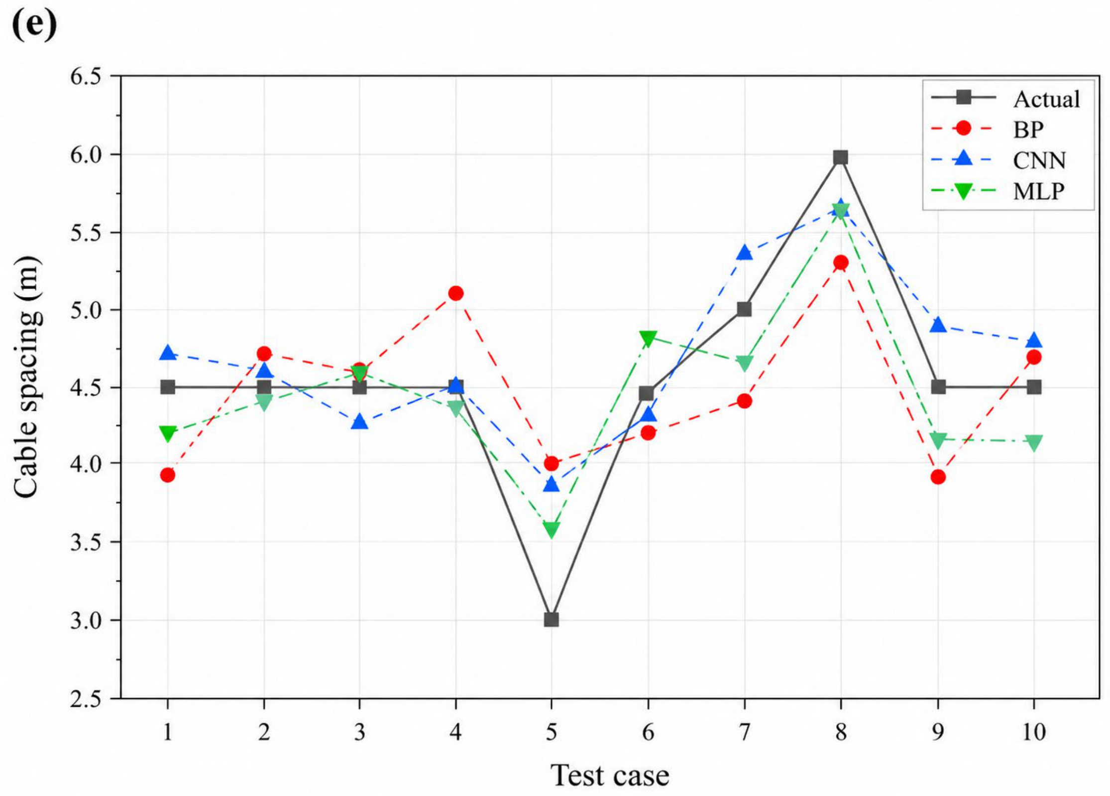
Figure 3 compares the predicted and real values of the five support parameters for the ten representative cases using the conventional models. The BP model shows noticeable deviations in several cases, particularly for cable force prediction. The CNN and MLP models generally follow the trend of the real values more closely.

Figure 3. Comparison of actual and predicted anchorage support parameters using conventional neural network models based on out-of-fold predictions from five-fold cross-validation for ten representative cases. (a) Bolt diameter (mm); (b) Bolt length (m); (c) Bolt spacing (m); (d) Cable design force (kN); (e) Cable spacing (m).

Figure 3 presents the out-of-fold predictions of the conventional BP, CNN, and MLP models for ten representative engineering cases. The five subplots correspond to bolt diameter, bolt length, bolt spacing, cable design force, and cable spacing. The predicted values are compared with the corresponding reference support parameters to illustrate differences in prediction behavior among the three models. Quantitative comparisons based on the complete five-fold cross-validation results are provided in Table 5.

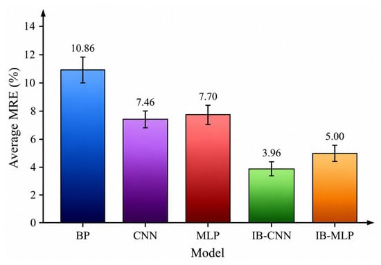
As shown in Figure 4 and Table 5, the BP model exhibited the highest average MRE (10.86%) among the three conventional neural network models. In comparison, the CNN and MLP models achieved average MREs of 7.46% and 7.70%, respectively. These results indicate that the CNN and MLP models provided more accurate overall predictions of the five anchorage support parameters than the BP model under the adopted five-fold cross-validation procedure.

Figure 4. Comparison of the average mean relative errors (MREs) of five prediction models based on five-fold cross-validation.

The differences in prediction accuracy among the conventional models may be associated with their network architectures and feature representation capabilities. Compared with the BP model, the CNN model employs convolutional operations and weight sharing to extract patterns from the input variables, whereas the MLP model uses a wider fully connected representation. These architectural differences may influence how the models learn nonlinear relationships from the limited engineering dataset. However, the present results do not isolate the individual contributions of network architecture, model capacity, and regularization; therefore, the observed performance differences should not be attributed to any single factor without further investigation.

4.2.2. Prediction Results of IB-Enhanced Neural Network Models

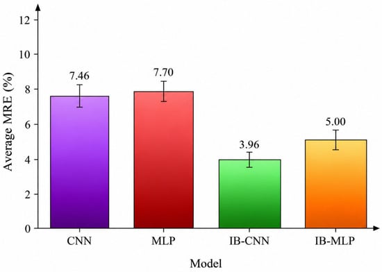
To evaluate the effectiveness of variational information bottleneck regularization, the IB-CNN and IB-MLP models were compared with their conventional counterparts. As shown in Table 5, IB-CNN reduced the average MRE from 7.46% to 3.96% relative to CNN, while IB-MLP reduced the average MRE from 7.70% to 5.00% relative to MLP. For cable design force, IB-CNN achieved an MRE of 5.91%, compared with 8.67% for IB-MLP.

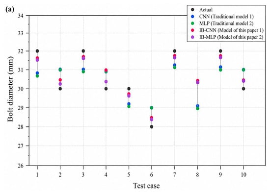
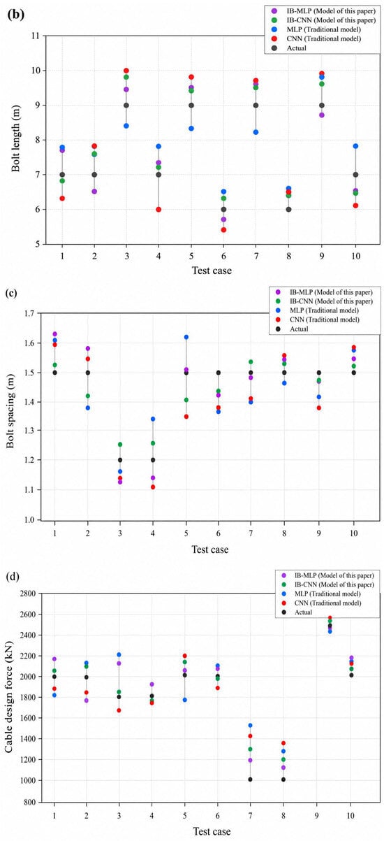
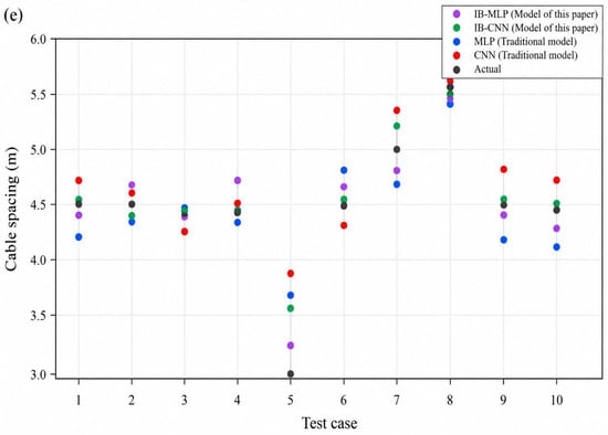
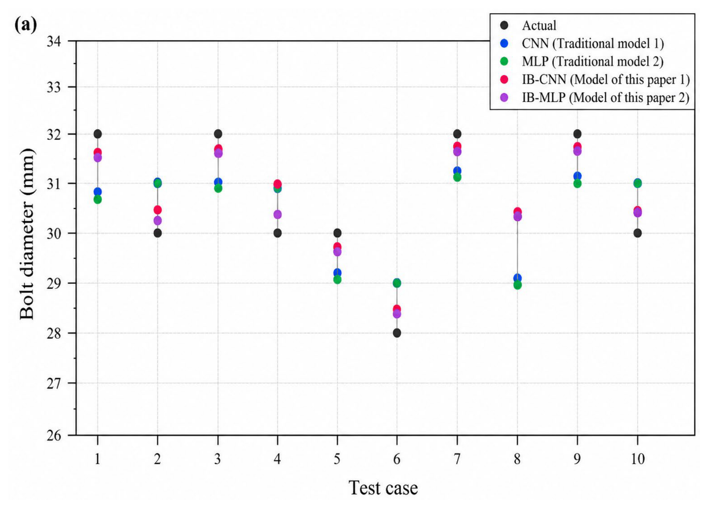
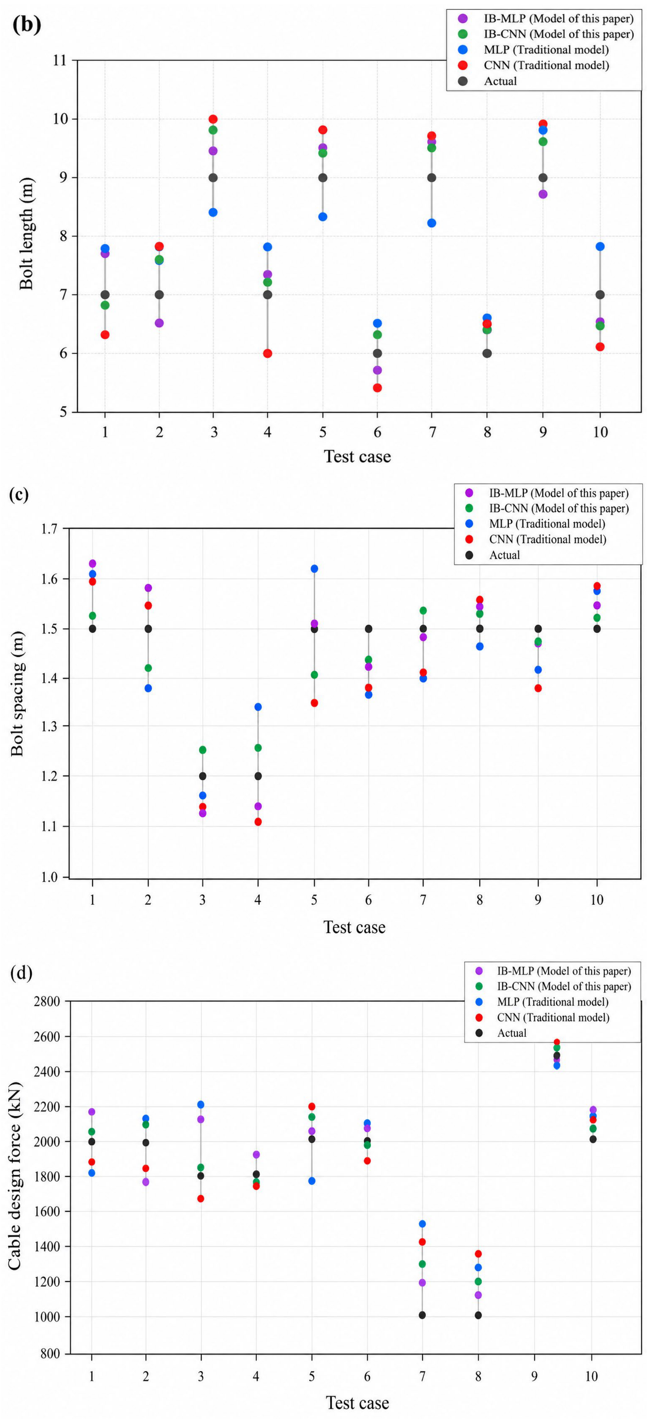
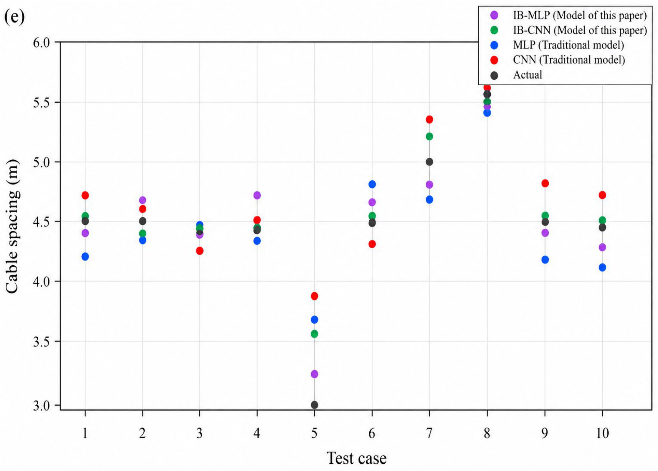
Figure 5 illustrates the predictions of the IB-enhanced models for ten representative engineering cases. These curves provide a qualitative comparison between predicted and reference support parameters, whereas the quantitative performance evaluation is based on the five-fold cross-validation results reported in Table 5.

Figure 5. Comparison of actual and predicted anchorage support parameters using the proposed models based on out-of-fold predictions from five-fold cross-validation. (a) Bolt diameter (mm); (b) Bolt length (m); (c) Bolt spacing (m); (d) Cable design force (kN); (e) Cable spacing (m).

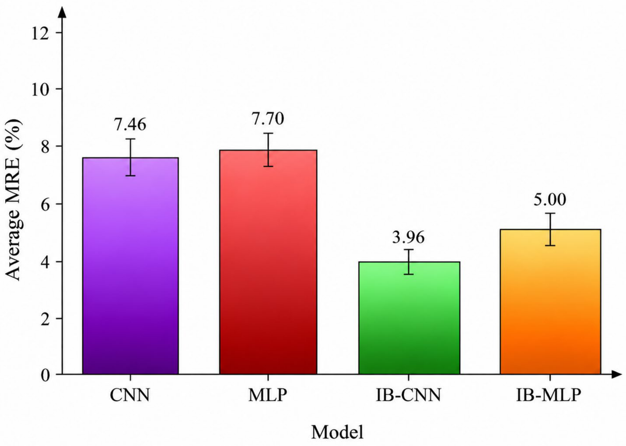
Figure 4 and Figure 6 compare the mean relative errors of the conventional and information bottleneck-enhanced models, respectively. The error bars represent the standard deviations of the fold-specific MRE values obtained from five-fold cross-validation, consistent with the statistical reporting in Table 5. Smaller error bars indicate less variation in prediction error across the evaluation folds. IB-CNN achieves the lowest average MRE among the evaluated models, indicating improved predictive accuracy under the adopted evaluation procedure.

Figure 6. Mean relative error of IB-enhanced neural network models.

The comprehensive evaluation metrics in Table 6 further demonstrate the predictive performance of the IB-enhanced models. IB-CNN achieved R² values of 0.94, 0.89, 0.87, 0.90, and 0.95 for bolt diameter, bolt length, bolt spacing, cable design force, and cable spacing, respectively. Its MAE and RMSE values were also lower than those of the conventional CNN model across all five prediction targets, indicating improved agreement between the predicted and reference support parameters.

Overall, the results demonstrate that the VIB regularization effectively improves the prediction accuracy and generalization capability of both CNN and MLP models under the limited-sample condition. The IB-CNN model consistently outperforms all other evaluated models and is selected for the engineering application demonstration in Section 4.3.

To investigate the contribution of the variational information bottleneck (VIB) mechanism, an ablation study was conducted using the same CNN and MLP backbone architectures. The investigated configurations included the unregularized baseline, dropout with a rate of 0.2, L2 weight decay with a coefficient of 1 × 10⁻⁴, a deterministic bottleneck with a latent dimension of 4, and a stochastic information bottleneck with β = 0. The proposed VIB configuration with β = 0.01 was also included. All configurations were evaluated using the same five-fold cross-validation partitions.

The deterministic bottleneck was used to examine the effect of feature compression without stochastic sampling or KL divergence regularization. The β = 0 configuration retained stochastic sampling while removing the KL divergence penalty, allowing the effects of stochastic representation learning and explicit information compression to be compared.

The VIB coefficient and bottleneck dimension were investigated through the parameter sensitivity analysis described in the subsequent section. In contrast, the dropout and L2 baselines were evaluated using fixed representative hyperparameter settings rather than independently optimized configurations. Therefore, the ablation results provide a comparison of the investigated configurations but do not establish that VIB would outperform all fully optimized conventional regularization methods.

In the ablation study, CNN and MLP were used as baseline models without the information bottleneck mechanism. IB-CNN and IB-MLP were developed by introducing the information bottleneck constraint into the corresponding baseline architectures while keeping the input variables, output parameters, and main network structures unchanged. Therefore, the performance differences mainly reflect the effect of the information bottleneck module (Table 7).

Table 7. Ablation study of different regularization strategies (average MRE over five outputs,%).

Model	CNN Backbone	MLP Backbone
Baseline (no regularization)	7.46 ± 0.47	7.70 ± 0.43
+Dropout (0.2)	6.52 ± 0.79	6.88 ± 0.85
+L2 weight decay (1 × 10−4)	6.81 ± 0.83	7.02 ± 0.88
+Deterministic bottleneck ($dim=4)$	5.96 ± 0.71	6.31 ± 0.76
+IB $\beta =0$	5.43 ± 0.65	5.87 ± 0.70
+IB ($\beta =0.01)$ [proposed]	3.96 ± 0.35	5.00 ± 0.44

The ablation results indicate that the VIB-enhanced models achieved lower prediction errors than the conventional regularization methods under the investigated settings. However, since dropout and L2 regularization were evaluated using fixed hyperparameters, these results do not necessarily demonstrate the superiority of VIB over fully optimized alternatives. Further hyperparameter comparisons are needed to confirm its general effectiveness (Table 8 and Table 9).

Table 8. Influence of the trade-off coefficient β on prediction performance (IB-CNN, average MRE over five outputs,%).

β	Bolt Diameter	Bolt Length	Bolt Spacing	Cable Force	Cable Spacing	Average
0.001	2.15 ± 0.42	7.82 ± 0.88	4.87 ± 0.61	8.56 ± 0.95	3.78 ± 0.52	5.44 ± 0.68
0.01	1.21 ± 0.28	5.29 ± 0.63	3.30 ± 0.41	5.10 ± 0.58	2.25 ± 0.33	3.96 ± 0.51
0.1	1.87 ± 0.35	6.15 ± 0.72	3.98 ± 0.49	6.34 ± 0.71	2.86 ± 0.40	4.24 ± 0.53
1	3.52 ± 0.51	8.76 ± 0.95	5.63 ± 0.68	10.21 ± 1.12	4.67 ± 0.58	6.56 ± 0.77

Table 9. Influence of the bottleneck dimension on prediction performance (IB-CNN, β = 0.01, average MRE over five outputs, %).

Bottleneck Dimension	Bolt Diameter	Bolt Length	Bolt Spacing	Cable Force	Cable Spacing	Average
2	1.68 ± 0.33	6.34 ± 0.74	4.12 ± 0.52	6.87 ± 0.79	3.12 ± 0.41	4.43 ± 0.56
4	1.21 ± 0.28	5.29 ± 0.63	3.30 ± 0.41	5.10 ± 0.58	2.25 ± 0.33	3.96 ± 0.51
6	1.35 ± 0.30	5.61 ± 0.66	3.52 ± 0.44	5.48 ± 0.62	2.47 ± 0.36	3.69 ± 0.48
8	1.52 ± 0.32	5.98 ± 0.70	3.78 ± 0.47	5.92 ± 0.67	2.71 ± 0.38	3.98 ± 0.51

The results show that the prediction performance is sensitive to both hyperparameters. For β, the performance improves from β = 0.001 to β = 0.01 but degrades when β becomes too large (β = 0.1 or 1). A very small β (0.001) provides insufficient compression and regularization, while an excessively large β (1) over-compresses the latent representation and loses prediction-relevant information. The value β = 0.01 achieves the best balance. For the bottleneck dimension, dimension 4 yields the lowest error. A dimension of 2 is too small to retain sufficient information, while dimensions 6 and 8 introduce redundant capacity that increases overfitting risk. The sensitivity analysis indicates that the prediction performance of the IB-CNN model varies with the information bottleneck coefficient β and the bottleneck dimension. Among the investigated candidate configurations, β = 0.01 and a bottleneck dimension of 4 yielded the lowest average MRE under the adopted cross-validation procedure.

It is worth noting that all models exhibit relatively larger prediction errors for Cases 7 and 8, where the real cable design force is 1000 kN—the lowest value in the dataset. For these two cases, the CNN model achieves cable force errors of approximately 35–40%, while the IB-CNN model reduces the errors to approximately 12–29%. This phenomenon can be attributed to two factors. First, 1000 kN lies at the lower boundary of the cable force distribution in the training data, and the majority of cases have cable forces of 1800–2500 kN. Neural networks generally perform poorly on out-of-distribution or boundary samples due to limited exposure during training. Second, low cable force designs typically correspond to favorable geological conditions, but the five input variables may not fully capture the specific engineering judgment that leads to a conservative low-force design. From an engineering application perspective, this indicates that the model should be used with caution for projects requiring low cable forces (≤1000 kN), and additional engineering judgment is necessary in such cases. The IB-CNN model, while still showing elevated errors for these cases, demonstrates better boundary generalization than the conventional CNN.

Furthermore, examination of the test cases reveals that the five input variables do not fully explain the variation in support design. For example, Case 6 is classified as Grade IV surrounding rock (the poorest among the test cases) yet employs the smallest bolts (28 mm diameter, 6 m length), while Case 9 is Grade II (good rock quality) but uses 32 mm diameter, 9 m length bolts and 2500 kN cables—the largest support scheme among the test cases. This apparent contradiction suggests that additional factors beyond the five input variables influence support design decisions, including the version of the design code used, the construction era and associated safety standards, the designer’s personal preference and risk attitude, the cavern functional type (main powerhouse vs. transformer room vs. tailwater tunnel), and the construction method (drill-and-blast vs. TBM). These unmodeled factors introduce inherent variability that limits the upper bound of prediction accuracy achievable with only five input parameters. Therefore, the prediction errors should not be interpreted solely as model deficiencies but also as a reflection of the multivariate nature of engineering support design. The proposed model captures the dominant trends driven by geological and geometric conditions but cannot account for project-specific design preferences.

A low relative prediction error does not necessarily guarantee correct bolt diameter selection because standard bolt diameters are discrete. Therefore, the predicted diameters were converted to the nearest available standard sizes (25, 28, 30, and 32 mm), as shown in Table 10. This comparison provides a more practical assessment of the model predictions for engineering applications.

Table 10. Standard specification matching accuracy based on five-fold cross-validation results.

Model	Bolt Diameter Accuracy	Cable Design Force Accuracy
BP	44.4% (8/18)	50.0% (9/18)
CNN	77.8% (14/18)	66.7% (12/18)
MLP	72.2% (13/18)	61.1% (11/18)
IB-CNN	94.4% (17/18)	83.3% (15/18)
IB-MLP	88.9% (16/18)	72.2% (13/18)

As shown in Table 10, the IB-CNN model achieved higher standard diameter matching accuracy than the conventional models for the evaluated cases. These results indicate that evaluating standard specification matching is important for assessing the engineering applicability of continuous model predictions.

4.3. Engineering Application Demonstration

To further demonstrate the engineering applicability of the proposed model, an underground powerhouse case of a hydropower station was selected as an application example. It should be explicitly noted that this demonstration case is included in the 121-case engineering database and was part of the training data in the five-fold cross-validation. Therefore, this example does not represent an independent validation dataset, but rather demonstrates the application workflow and output interpretation of the proposed model as an auxiliary tool for preliminary anchorage parameter selection. The predicted values reported in this section are obtained from the IB-CNN model trained on the full dataset (all 121 cases), which may differ slightly from the cross-validation predictions reported in Section 4.2 due to the larger training set size (Table 11 and Table 12).

Table 11. Input parameters for the demonstration case.

Input Parameter	Unit	Main Plant	Transformer Room
Rock mass classification	—	III	III
Excavation span	m	27.5	20.5
Excavation height	m	61.0	36.0
UCS	MPa	105.0	110.0
Maximum principal stress	MPa	18.0	18.0

Table 12. Existing Anchorage Support Parameters of the Demonstration Case.

Place	Bolt Diameter/mm	Bolt Length/m	Bolt Spacing/m	Cable Design Force/kN	Cable Spacing/m
Main Plant	32	7	1.5	2000	4.5
Main Transformer Room	28	8	1.5	2000	4.5

The demonstration case includes two representative underground cavern locations: the Main Plant and the Main Transformer Room. The adopted support schemes show that the engineering design uses relatively large bolt diameters, long anchorage lengths, and high cable design forces, reflecting the requirement for reinforcement of large underground caverns.

Based on the comparative results presented in Section 4.2, the IB-CNN model was selected to illustrate the preliminary anchorage support parameter prediction workflow. The model was retrained using all 121 available engineering cases, and its outputs for the demonstration case are presented in Table 13 and Table 14. Because the demonstration case was included in the training dataset, these results are intended solely to illustrate the model application procedure and the interpretation of continuous predictions. They should not be regarded as independent evidence of predictive generalization or engineering design reliability.

Table 13. Predicted Anchorage Support Parameters Using the IB-CNN Model.

Place	Bolt Diameter/mm	Bolt Length/m	Bolt Spacing/m	Cable Design Force/kN	Cable Spacing/m
Main Plant	31.46	7.18	1.47	1952	4.42
Main Transformer Room	28.35	7.76	1.48	2048	4.57

Table 14. Relative deviation between predicted and existing support parameters.

Engineering Case	Parameter	Existing	Prediction	Relative Error
Main Plant	Bolt diameter	32	31.46	1.69%
	Bolt length	7	7.18	2.57%
	Bolt spacing	1.5	1.47	2.00%
	Cable design force	2000	1952	2.40%
	Cable spacing	4.5	4.42	1.78%
Main Transformer Room	Bolt diameter	28	28.35	1.25%
	Bolt length	8	7.76	3.00%
	Bolt spacing	1.5	1.48	1.33%
	Cable design force	2000	2048	2.40%
	Cable spacing	4.5	4.57	1.56%

As shown in Table 13 and Table 14, the predicted anchorage support parameters are close to the values adopted in the existing engineering design. The relative deviations range from 1.25% to 3.00% across the two cavern locations, with the largest deviation observed for bolt length in the Main Transformer Room (3.00%). The relatively small deviations indicate close numerical agreement with the existing support parameters, but they do not independently establish engineering design acceptability. Nevertheless, because the demonstration case was included in the model training dataset, these results should be interpreted as an illustration of the prediction workflow rather than independent validation of engineering applicability. The predicted parameters require further verification against project-specific design requirements and engineering safety constraints before practical adoption.

Conventional support design methods, such as the Q-system, provide engineering guidance based on rock mass conditions and established design criteria. In contrast, the proposed IB-CNN model predicts anchorage support parameters by learning nonlinear relationships from engineering data. A direct quantitative comparison was not conducted because the available dataset does not contain all the parameters required to independently apply these conventional methods. Therefore, the proposed model should be regarded as an auxiliary tool for preliminary support parameter estimation rather than a replacement for code-based engineering design and verification.

5. Conclusions

This study developed neural-network-based prediction models for anchorage support parameter estimation of underground caverns using engineering geological and support datasets. CNN and MLP models were established as baseline models, and the variational information bottleneck (VIB) method was introduced as a regularization strategy to improve feature representation under small-sample conditions. The main conclusions are summarized as follows:

(1) A machine-learning framework was established to predict five anchorage support parameters, including bolt diameter, bolt length, bolt spacing, cable design force, and cable spacing, based on five geological and engineering variables. CNN and MLP models were used to capture the nonlinear relationship between geological conditions and support parameters, while IB-enhanced models were constructed by introducing a bottleneck representation and KL-divergence regularization.

(2) Under the adopted five-fold cross-validation procedure, the information-bottleneck-enhanced CNN and MLP models achieved lower mean relative errors than their corresponding conventional backbone models. The ablation results suggest that bottleneck-based representation learning and KL divergence regularization may contribute to improved predictive performance under the investigated configurations. However, the individual contributions of these mechanisms have not been fully isolated.

(3) Among the investigated model configurations, IB-CNN achieved the lowest reported average mean relative error, followed by IB-MLP. These findings suggest that the variational information bottleneck is a promising strategy for improving anchorage support parameter prediction with limited engineering data. Nevertheless, because hyperparameters were selected using the same cross-validation folds employed for performance reporting, the results may be affected by model-selection bias and should not be interpreted as fully independent estimates of generalization performance.

(4) An underground powerhouse case included in the engineering database was used to demonstrate the prediction workflow. The IB-CNN predictions showed relatively small numerical deviations from the existing support parameters. This comparison illustrates the potential of the model as an auxiliary tool for preliminary parameter estimation, but it does not constitute independent external validation or establish the engineering safety and design adequacy of the predicted support scheme.

Despite the promising performance of the proposed models, several limitations remain. The current dataset is limited to 121 engineering cases, and further validation using larger and more diverse datasets is required to improve the generalization capability of the models. In addition, although five-fold cross-validation was adopted to evaluate model performance, independent validation under different geological conditions is still necessary. Future studies will focus on expanding the database and investigating the applicability of the proposed approach in more complex engineering scenarios.

References

- Wang, T.; Fan, B.; Khadka, S.S. Flowchart of DEM Modeling Stability Analysis of Large Underground Powerhouse Caverns. Adv. Civ. Eng. 2020, 8874120. [Google Scholar]
- Peng, X.C. Study on the construction organisation of underground plant excavation of Shuangjiangkou Hydropower Station. Sichuan Hydropower 2016, 35, 76–80. [Google Scholar]
- Zhang, Q.; Zheng, Y. Geotechnical Investigations and Support Design for an Underground Powerhouse of Pumped-Storage Power Station: A Case Study in Chongqing, China. Sustainability 2022, 14, 8481. [Google Scholar] [CrossRef] [Scilit]
- Yang, Z.; Zhang, K.; Li, Y.; Xie, L.; Cao, S.; Zhang, Q. Optimization of Rock Bolt Support Parameters for TBM Tunnels in High In-Situ-Stress Soft Rock Based on Deformation and Stress Evolution Analysis. Front. Earth Sci. 2026, 14, 1825720. [Google Scholar] [CrossRef] [Scilit]
- Van Kien, D. Numerical simulation of the stability of rock mass around large underground cavern. Civ. Eng. J. 2022, 8, 81–91. [Google Scholar] [CrossRef] [Scilit]
- Ma, K.; Zhang, J.; Zhou, Z.; Xu, N. Comprehensive analysis of the surrounding rock mass stability in the underground caverns of Jinping I hydropower station in Southwest China. Tunn. Undergr. Space Technol. 2020, 104, 103525. [Google Scholar] [CrossRef] [Scilit]
- Zhu, W.S.; Li, X.J.; Zhang, Q.B.; Zheng, W.H.; Xin, X.L.; Sun, A.H.; Li, S.C. A study on sidewall displacement prediction and stability evaluations for large underground power station caverns. Int. J. Rock Mech. Min. Sci. 2010, 47, 1055–1062. [Google Scholar] [CrossRef] [Scilit]
- Ren, Q.; Xu, L.; Zhu, A.; Shan, M.; Zhang, L.; Gu, J.; Shen, L. Comprehensive safety evaluation method of surrounding rock during underground cavern construction. Undergr. Space 2021, 6, 46–61. [Google Scholar] [CrossRef] [Scilit]
- Liu, X.Y.; Xu, D.P.; Jiang, Q.; Ma, X.D. Excavation response and reinforcement practice of large underground caverns within high-stress hard rock masses: The case of Shuangjiangkou hydropower Station, China. Tunn. Undergr. Space Technol. 2024, 147, 105698. [Google Scholar] [CrossRef] [Scilit]
- Cheng, Y.; He, Z.; Zeng, X.; Hu, S.; Chu, W. Back analysis of rock mechanical parameters of underground caverns based on multi-layer perceptron regression algorithm. In Third International Conference on Electronic Information Engineering and Data Processing (EIEDP 2024); SPIE: Breda, The Netherlands, 2024; Volume 13184, pp. 816–822. [Google Scholar]
- Zhang, K.; Lyu, H.M.; Shen, S.L.; Zhou, A.; Yin, Z.Y. Evolutionary hybrid neural network approach to predict shield tunneling-induced ground settlements. Tunn. Undergr. Space Technol. 2020, 106, 103594. [Google Scholar] [CrossRef] [Scilit]
- Reddy, Y.R. Forecasting Displacement of Underground Caverns Using Machine Learning Techniques. Int. J. Creat. Res. Thoughts. 2020, 8, 3438–3441. Available online: https://ijcrt.org/viewpaperforall.php?paper=IJCRT2012381 (accessed on 13 October 2026).
- Mahdevari, S.; Torabi, S.R. Prediction of tunnel convergence using artificial neural networks. Tunn. Undergr. Space Technol. 2012, 28, 218–228. [Google Scholar] [CrossRef] [Scilit]
- Adoko, A.C.; Jiao, Y.Y.; Wu, L.; Wang, H.; Wang, Z.H. Predicting tunnel convergence using multivariate adaptive regression spline and artificial neural network. Tunn. Undergr. Space Technol. 2013, 38, 368–376. [Google Scholar] [CrossRef] [Scilit]
- Zhang, P.; Wu, H.N.; Chen, R.P.; Chan, T.H.T. Hybrid meta-heuristic and machine learning algorithms for tunneling-induced settlement prediction: A comparative study. Tunn. Undergr. Space Technol. 2020, 99, 103383. [Google Scholar] [CrossRef] [Scilit]
- Mulumba, D.M.; Liu, J.; Hao, J.; Zheng, Y.; Liu, H. Application of an optimized PSO-BP neural network to the assessment and prediction of underground coal mine safety risk factors. Appl. Sci. 2023, 13, 5317. [Google Scholar] [CrossRef] [Scilit]
- Cao, W.; Jiang, Y.; Sakaguchi, O.; Li, N.; Han, W. Predication of displacement of tunnel rock mass based on the back-analysis method-BP neural network. Geotech. Geol. Eng. 2022, 40, 531. [Google Scholar] [CrossRef] [Scilit]
- Liang, M.; Hu, C.; Yu, R.; Wang, L.; Zhao, B.; Xu, Z. Optimization of the process parameters of fully mechanized top-coal caving in thick-seam coal using BP neural networks. Sustainability 2022, 14, 1340. [Google Scholar] [CrossRef] [Scilit]
- Shuguang, L.; Yanjun, S.; Peng, L.; Jiangsheng, X.; Sisi, T.; You, L.; Wen, M. Classification method of surrounding rock of plateau tunnel based on BP neural network. Front. Earth Sci. 2023, 11, 1283520. [Google Scholar] [CrossRef] [Scilit]
- Ambrožič, T.; Turk, G. Prediction of subsidence due to underground mining by artificial neural networks. Comput. Geosci. 2003, 29, 627–637. [Google Scholar] [CrossRef] [Scilit]
- Özyurt, M.C.; Karadogan, A. A new model based on artificial neural networks and game theory for the selection of underground mining method. J. Min. Sci. 2020, 56, 66–78. [Google Scholar] [CrossRef] [Scilit]
- Jiang, F.; Zhou, K.; Deng, H.; Li, X.; Zhong, Y. An Optimized Model for Blasting Parameters in Underground Mines’ Deep-Hole Caving Based on Rough Set and Artificial Neural Network. In 2009 Second International Symposium on Computational Intelligence and Design; IEEE: New York, NY, USA, 2009; Volume 1, pp. 459–462. [Google Scholar]
- Samadi, H.; Alanazi, A.; Muhodir, S.H.; Alsubai, S.; Alqahtani, A.; Marzougui, M. In-depth exploration of machine learning algorithms for predicting sidewall displacement in underground caverns. Geomech. Eng. 2024, 37, 307–321. [Google Scholar]
- Keawsawasvong, S.; Seehavong, S.; Ngamkhanong, C. Application of artificial neural networks for predicting the stability of rectangular tunnels in Hoek–Brown rock masses. Front. Built Environ. 2022, 8, 837745. [Google Scholar] [CrossRef] [Scilit]
- Tishby, N.; Pereira, F.C.; Bialek, W. The information bottleneck method. arXiv 1999, arXiv:physics/0004057. [Google Scholar]
- Alemi, A.A.; Fischer, I.; Dillon, J.V.; Murphy, K. Deep variational information bottleneck. arXiv 2016, arXiv:1612.00410. [Google Scholar]
- Shwartz-Ziv, R.; Tishby, N. Opening the black box of deep neural networks via information. arXiv 2017, arXiv:1703.00810. [Google Scholar]
- Goldfeld, Z.; Polyanskiy, Y. The information bottleneck problem and its applications in machine learning. IEEE J. Sel. Areas Inf. Theory 2020, 1, 19–38. [Google Scholar] [CrossRef] [Scilit]
- Slonim, N.; Friedman, N.; Tishby, N. Multivariate information bottleneck. Neural Comput. 2006, 18, 1739–1789. [Google Scholar] [CrossRef] [Scilit]
- Zaidi, A.; Estella-Aguerri, I.; Shamai, S. On the information bottleneck problems: Models, connections, applications and information theoretic views. Entropy 2020, 22, 151. [Google Scholar] [CrossRef] [Scilit]
- Tang, P.; Peng, K.; Dong, J. Nonlinear quality-related fault detection using combined deep variational information bottleneck and variational autoencoder. ISA Trans. 2021, 114, 444–454. [Google Scholar] [CrossRef] [Scilit]
Disclaimer/Publisher’s Note: The statements, opinions and data contained in all publications are solely those of the individual author(s) and contributor(s) and not of MDPI and/or the editor(s). MDPI and/or the editor(s) disclaim responsibility for any injury to people or property resulting from any ideas, methods, instructions or products referred to in the content. |
© 2026 by the authors. Licensee MDPI, Basel, Switzerland. This article is an open access article distributed under the terms and conditions of the Creative Commons Attribution (CC BY) license.