


Abstract
Accurately reconstructing consecutive missing measurement segments presents a major challenge in bridge structural health monitoring, due to the inherent complexity and non-stationary nature of the collected signals. To address this, a hybrid data recovery framework is developed by integrating Improved Complete Ensemble Empirical Mode Decomposition with Adaptive Noise, Permutation Entropy, Long Short-Term Memory networks, and the Informer model (ICEEMDAN-PE-LSTM-Informer). The process begins by employing ICEEMDAN-PE to decompose the raw monitoring data into multiscale intrinsic mode components with distinct temporal characteristics. Subsequently, a parallel LSTM-Informer architecture is designed to forecast each decomposed component independently. This dual-branch design combines the local temporal modeling capability of LSTM with the long-range dependency modeling capability of Informer, and the extracted features are fused through a fully connected layer before prediction. The final recovered data sequence is obtained by linearly aggregating the predicted results from all components. The proposed method is evaluated using complete bearing-displacement and strain records from an operational bridge SHM system. Because the original datasets contain no missing observations, consecutive missing intervals are artificially constructed in the test sequences by controlled masking, allowing the original measurements to serve as ground truth for quantitative evaluation. Experimental results demonstrate improved reconstruction accuracy for the two bridge-monitoring datasets considered in this study. Specifically, for the longest prediction horizon of 72 steps, corresponding to a 12 h consecutive missing interval, the RMSE values for recovering bearing displacement and strain data are decreased by 54.06% and 44.11%, respectively, compared to a standard LSTM model, and by 46.06% and 31.47% compared to the standalone Informer model. These findings indicate that the proposed ICEEMDAN-PE-LSTM-Informer framework provides improved reconstruction performance over the considered baseline models for the two structural-response datasets investigated in this study.
1. Introduction
Throughout their operational lifespan, bridges experience a diverse range of environmental and mechanical stresses, such as temperature variations, vehicular traffic, wind forces, and additional dynamic influences. These cumulative effects result in the progressive deterioration of structural integrity, thereby introducing significant safety concerns. As a pivotal solution, Structural Health Monitoring (SHM) systems provide continuous, real-time surveillance of bridge conditions, allowing for the early identification of possible structural impairments and operational anomalies [1]. However, monitoring data is often distorted or lost due to sensor deterioration, storage failures, and other issues [2,3]. Missing data leads to inaccurate evaluations of structural performance and undermines the effectiveness of safety decisions [4,5]. Therefore, accurate and complete measurement data are crucial for the safety assessment of bridge structures, highlighting the necessity to develop an efficient and feasible method for data recovery.
The reconstruction of incomplete measurement data mainly relies on two approaches: finite element model-based techniques and data-driven methodologies [6]. The former adjusts an initial finite element model by incorporating available measured data to infer missing information. For instance, Li et al. [7] utilized seismic response monitoring data from a continuous straight highway bridge in Chile to update the bridge’s initial finite element model and subsequently reconstructed responses not captured during the earthquake. Hu et al. [8] introduced an integrated framework for multi-sensor placement and structural response reconstruction. Through experiments on a cantilever beam instrumented with multiple sensor types, they optimized sensor locations and successfully reconstructed responses at critical structural positions. Furthermore, Li et al. [9] proposed a two-degree multiscale finite element model based on singular value decomposition theory, which effectively reconstructed both displacement and strain–stress responses of the structure. These studies confirm that the finite element-based approach possesses clear practical relevance and physical interpretability, enabling accurate data recovery. Nevertheless, its applicability is often constrained due to the high dependency of reconstruction accuracy on parameters defined in the finite element model. Uncertainties and simplifications inherent in the modeling process—such as assumptions regarding boundary conditions and material properties—can compromise the model’s predictive reliability. Consequently, research employing this method tends to focus on relatively simpler bridge configurations [10,11]. In comparison, data-driven methods do not require detailed modeling of the underlying physical mechanisms. Instead, they restore missing data by extracting patterns from large volumes of monitoring records. This modeling paradigm offers greater flexibility and adaptability, providing notable advantages in addressing the practical intricacies associated with real-world bridge structures and their monitoring systems [12].
Broadly speaking, data-driven approaches for missing data recovery can be categorized into three groups: methods based on sparse representation [13], those relying on statistical analysis [14], and techniques employing deep learning [15]. Thanks to the rapid progress in computing and artificial intelligence, current research increasingly favors deep learning-based strategies. For example, Oh et al. [16] designed a convolutional neural network (CNN) that effectively reconstructed the strain response of a failed sensor by utilizing only strain data from other functioning sensors. Similarly, Lu et al. [17] adopted the concept of high-frequency bridge dynamics and applied a back-propagation artificial neural network (BP-ANN) to rebuild the bridge’s high-frequency response. In recent years, recurrent neural networks (RNNs) and their variants—such as long short-term memory (LSTM) and gated recurrent unit (GRU) networks—have gained popularity for data recovery tasks. Their ability to retain temporal dependencies makes them particularly effective for addressing sequential data issues [18,19]. To further improve prediction precision, various researchers have focused on optimizing these network architectures [20,21]. Nevertheless, even these advanced models are limited by inherent memory mechanisms that can lead to information decay and difficulty in capturing long-range dependencies. As a result, their effectiveness in long-term forecasting scenarios remains constrained.
To overcome these constraints, encoder–decoder architectures have gained growing interest. In 2017, Vaswani et al. [22] proposed the Transformer model, which re-duces the difficulties of capturing long-range sequence dependencies faced by conventional RNNs through the use of residual connections and layer normalization. However, this architecture also presents drawbacks such as significant computational overhead, reduced efficiency, and the accumulation of stepwise errors during inference. In response, Zhou et al. [23] later presented an enhanced variant called Informer, which tackles these shortcomings by integrating a Sparse Self-Attention Mechanism with Probabilistic Constraints, a self-attention distilling operation, and a generative decoding strategy applied in a single forward pass. These improvements make Informer more capable of handling long-sequence time series forecasting [24,25]. As a result, researchers have begun investigating its potential for reconstructing missing data. For example, Wang et al. [26] proposed a Bidirectional Penalty-Informer model for recovering lengthy missing sequences in forest ecological data, evaluating it under both univariate and multivariate missing scenarios. Their results showed that this model achieved greater prediction accuracy and robustness compared to existing methods. Despite Informer’s strong performance in long-term forecasting, its effectiveness in short-term prediction tasks is often limited and can even fall short of that achieved by LSTM models [24]. Given this shortcoming, researchers have explored hybrid approaches that integrate Informer with other deep learning architectures, applying these combined models to various time series forecasting problems [25,27,28]. Empirical outcomes confirm that such integrated frameworks perform effectively, consistently surpassing the prediction accuracy of the standalone Informer model.
While the models mentioned previously deliver notable predictive performance, they often exhibit limitations in handling nonlinear data patterns [29]. In light of this, researchers have increasingly turned to integrating signal processing methods with deep learning frameworks, adopting hybrid modeling strategies to enhance time series forecasting accuracy, with promising outcomes reported [30,31,32]. Recognizing the strengths of these integrated approaches, several studies have applied them to missing data recovery. By framing the data reconstruction task as a sequential prediction problem, various hybrid models have been introduced, such as EMD-LSTM [33], TVFEMD-CNN-GRU [34], and TVFEMD-ED-LSTM [15]. Although decomposition techniques utilized in these studies can improve the performance of prediction models to some degree, certain methods—including Empirical Mode Decomposition (EMD) and Ensemble EMD (EEMD)—still suffer from mode mixing issues. To address this, an enhanced approach termed Improved Complete Ensemble Empirical Mode Decomposition with Adaptive Noise (ICEEMDAN) has been proposed [35]. ICEEMDAN effectively reduces residual noise in each decomposed component through adaptive noise regulation, thereby partially mitigating the problem of mode mixing. Its robust performance has led to growing application in areas such as time series forecasting and fault diagnosis [36,37]. Nevertheless, the use of ICEEMDAN in reconstructing missing bridge monitoring data remains underexplored, indicating a clear need for further investigation and adaptation of this technique within the field of bridge structural health monitoring.
As summarized in Table 1, previous decomposition-assisted recovery methods have demonstrated the effectiveness of combining signal decomposition with recurrent or convolution–recurrent predictors. However, the comparison also highlights three issues that remain relevant to long consecutive missing-data reconstruction. First, decomposition quality directly affects downstream prediction, while some EMD-family methods remain susceptible to mode mixing or decomposition uncertainty. Second, most decomposition-assisted workflows predict individual modal components directly, without an explicit complexity-guided regrouping stage to reduce the heterogeneity of the prediction targets. Third, recurrent or convolution–recurrent predictors primarily emphasize local and sequential dependence, whereas long consecutive gaps also require effective modeling of longer-range temporal relationships. These observations motivate the coordinated use of ICEEMDAN decomposition, PE-guided component regrouping, and parallel LSTM-Informer modeling adopted in this study.
Table 1.
Comparison of representative data recovery methods relevant to long consecutive missing measurements.
From the perspective of long consecutive missing-data reconstruction, the above approaches exhibit distinct strengths and limitations. Conventional interpolation, statistical, and sparse-representation methods are generally computationally inexpensive and interpretable and can be effective for isolated or relatively short missing intervals. However, their performance can deteriorate when a long consecutive block is unavailable because few or no observations exist inside the gap to constrain the reconstruction, and assumptions of local smoothness, stationarity, or sparse correlation may no longer adequately represent nonlinear and non-stationary bridge responses. Recurrent models such as LSTM and GRU can learn nonlinear temporal dependencies directly from monitoring data and are therefore more suitable for sequential recovery, but their finite-memory mechanism may weaken the transmission of information as the missing horizon increases. Transformer-based models alleviate this limitation through attention mechanisms that capture longer-range dependencies; however, conventional Transformers incur relatively high computational cost, and attention-based models may not be equally effective at representing short-term local fluctuations. Decomposition-based methods provide another strategy by separating a nonlinear and non-stationary monitoring signal into simpler multiscale components before prediction, thereby reducing the learning difficulty of the downstream model. Nevertheless, decomposition itself does not reconstruct the missing sequence, and its effectiveness depends on the decomposition quality; EMD-family methods may suffer from mode mixing, while decomposition-assisted frameworks also introduce additional computational cost. Existing hybrid models attempt to combine these complementary advantages, but their increased structural complexity makes it difficult to determine whether performance gains arise from the decomposition stage, component regrouping, or the subsequent predictor. These limitations become particularly relevant for long consecutive missing intervals, for which both local temporal variations and long-range dependencies must be preserved while avoiding excessive preprocessing and modeling uncertainty.
These observations indicate that no single existing modeling paradigm simultaneously addresses all of the challenges associated with long consecutive missing-data reconstruction. For bridge-monitoring signals, recurrent models are advantageous for local and short-term temporal dependence, whereas attention-based models are more suitable for longer-range relationships. Meanwhile, decomposition can reduce the non-stationarity and multiscale complexity of the original signal, but its contribution should be separated from that of the prediction architecture. Therefore, an effective recovery framework for long consecutive gaps should combine multiscale preprocessing with complementary local- and long-range temporal modeling, while allowing the contribution of each major component to be evaluated explicitly.
To address the above limitations, this study develops an ICEEMDAN-PE-LSTM-Informer framework for the reconstruction of consecutive missing measurements in bridge SHM. The original monitoring sequence is first decomposed using ICEEMDAN, and permutation entropy is then employed to reorganize the resulting IMFs into components with different temporal characteristics. For each reconstructed component, LSTM and Informer are arranged in parallel so that local/short-term temporal dependence and long-range dependence can be extracted simultaneously, after which the two feature representations are fused to produce the component prediction. Finally, the predicted components are superimposed to obtain the reconstructed monitoring sequence. The framework is evaluated using bearing-displacement and strain records from the Badahe Bridge SHM system.
The main contributions of this study are summarized as follows:
- (1)
- A complexity-guided multiscale preprocessing strategy is developed to reduce the heterogeneity of decomposed bridge-monitoring signals. Rather than directly predicting each IMF independently, ICEEMDAN is followed by PE-based regrouping so that IMFs with similar temporal complexity are combined into a fixed number of reconstructed components. This design also allows correspondence between independently decomposed training and test sequences to be established at the reconstructed-component level, even when the numbers of original IMFs differ.
- (2)
- A parallel LSTM-Informer architecture is introduced for each reconstructed component to address the different temporal scales involved in long consecutive-gap recovery. The LSTM branch emphasizes local and short-term temporal evolution, whereas the Informer branch captures longer-range dependencies through ProbSparse self-attention. Their features are fused before output rather than relying on a single predictor to model both temporal regimes.
- (3)
- The contribution and practical characteristics of the proposed framework are evaluated from multiple perspectives rather than prediction accuracy alone. In addition to comparisons with LSTM, CNN-LSTM, Informer, LSTM-Informer, and CEEMDAN-PE-LSTM-Informer, the revised study includes component-wise ablation analysis, sequence-length sensitivity analysis, and computational-cost evaluation. The method is examined using two different structural response records from the same operational bridge and under multiple consecutive missing-data lengths.
1.1. ICEEMDAN Algorithm
ICEEMDAN is developed based on CEEMDAN [35]. As a key improvement over CEEMDAN, the ICEEMDAN method incorporates the k-th modal component of white noise subsequent to the implementation of EMD, which can efficiently tackle the defects of residual noise and spurious modes inherent in the original CEEMDAN framework. The specific decomposition procedure is described as follows:
We define as the target signal for decomposition. Here, refers to the modal component obtained via the EMD approach, and stands for the local average value of the original signal generated through the EMD method.
Step 1: Adding a set of Gaussian white noise to the original signal gives a new signal as:
where is the standard deviation of Gaussian white noise added during the first signal decomposition.
Step 2: When , the first residual and the first modal component are obtained:
Step 3: When , the local mean of is calculated by EMD plus Gaussian white noise, and the second residual value and the second modal component are obtained:
Step 4: Similarly, when , the residual and the modal component are obtained:
where is the standard deviation of Gaussian white noise added during the signal decomposition.
Step 5: Repeat Step 4 until the decomposition is complete to obtain all modal components and residual components.
1.2. PE Algorithm
PE [38] can effectively measure the complexity of time series. This algorithm does not require a long sequence length and has good anti-noise ability. For a given time series of length , the detailed calculation procedures are presented as follows:
Step 1: Set the embedding dimension and the delay time .
Step 2: Through the phase space reconstruction of the original time series, several subsequences are obtained, such as .
Step 3: By comparing the values of the internal elements, is arranged in ascending order according to the rule of , and a set of symbol sequences is obtained.
Step 4: Compute the probability of the occurrence of the symbol sequence, and further compute the PE of the time series , where .
Step 5: The calculated PE is normalized: . The closer the value is to 0, the more regular the time series.
In the present framework, PE is not used to determine the absolute frequency of an IMF. The IMFs generated by ICEEMDAN are intrinsically arranged from relatively high-frequency/short-scale components to low-frequency/long-scale components. PE is instead employed as a quantitative indicator of the temporal complexity of each IMF and is used to determine the boundaries for component regrouping.
After calculating the normalized PE value of each IMF, the difference between two adjacent frequency-ordered IMFs is calculated as . The two largest adjacent PE differences are selected as the two regrouping boundaries and . The reconstructed components are consequently defined as
This criterion is data-adaptive and therefore does not require fixed empirical PE thresholds. The same calculation procedure and PE parameters ( and ) are applied independently to all datasets. Consequently, the numerical PE values and the number of IMFs within each reconstructed component may differ among datasets, while the regrouping criterion remains unchanged.
1.3. Prediction Model Based on LSTM-Informer
1.3.1. LSTM Model
Recurrent Neural Network (RNN) refers to a neural network architecture characterized by state memory capability, where the network’s output at any given moment is associated not only with the current input but also with the input from the preceding time step. For this reason, RNNs are widely employed in tasks related to sequence recognition and temporal prediction. Nevertheless, during the training phase, this model is prone to issues like gradient vanishing or gradient exploding, which impede its ability to capture long-term historical data information [39]. To tackle these above-mentioned drawbacks, a distinctive “gate” mechanism is incorporated to control the flow of information, thereby giving rise to the Long Short-Term Memory (LSTM) network [40].
As illustrated in Figure 1, the core principle of the LSTM model lies in the adoption of three gating mechanisms—the input gate, forget gate, and output gate—to govern the transmission of information.
Figure 1.
Model and modules of the LSTM.
The forget gate takes the previous hidden state and the current input as inputs. A sigmoid activation maps the output to the interval , thereby controlling the proportion of information retained from the previous cell state. The forget gate is calculated as
In this context, stands for the sigmoid activation function, with and being the weight matrix and bias vector of the forget gate, respectively.
The input gate performs selective updates on information and then stores the updated content in the cell state, whose corresponding expression is given as follows:
where is the input gate, is the candidate memory unit, is a hyperbolic tangent activation function, and are the weight parameter matrices, and are bias vectors.
The output gate leverages the sigmoid function to decide which specific information is to be incorporated into the computation of the subsequent time step. The formula for the output gate is as shown:
where and are the weight parameter matrix and bias vector of the output gate, respectively.
Finally, the current moment memory unit state and hidden state are updated based on the results of the forget gate, input gate, and output gate, as shown in Equations (12) and (13).
1.3.2. Informer Model
As an efficient forecasting model derived from the Transformer architecture, the Informer is designed to address the issue of excessive computational complexity inherent in the self-attention mechanism while boosting the model’s predictive performance [23]. In contrast to the original Transformer model, the Informer incorporates two key mechanisms: the ProbSparse self-attention mechanism and the self-attention distilling mechanism. These components serve to cut down the computational complexity of time series processing and elevate the overall computational efficiency of the model. Moreover, the Informer adopts a generative decoder, which enables the acquisition of all predicted values in a single forward pass. This design not only accelerates the forecasting speed but also alleviates the propagation of cumulative errors during the prediction process. The architectural framework of the Informer model is depicted in Figure 2.
Figure 2.
The structure of the Informer model.
- (1)
- Input of the Informer
Unlike the input representation in the Transformer, the Informer retains the scalar value encoding and local time encoding from the Transformer while incorporating global time encoding. This design enhances the model’s ability to extract periodic patterns and evolving trends from time series data. Specifically, scalar value encoding employs 1D convolution to execute scalar projection on the input sequence. Local time encoding utilizes fixed-position coding in the Transformer, which encodes information using sine and cosine terms to retain local information. Additionally, global time encoding considers the temporal patterns in the data and extracts features such as month, week, hour, and minute from the data timestamp to construct the global time feature. Finally, the above features extracted by the three encoding approaches are summed as the input of the Informer.
- (2)
- Multi-head ProbSparse self-attention mechanism
The quadratic increase in computational complexity with sequence length in standard self-attention can dilute the model’s focus on critical information [41]. To address this, the Informer employs a novel ProbSparse self-attention mechanism, leveraging the long-tail distribution observed in attention feature maps. During the computation process, it selectively focuses on the significant components of the query vector to calculate attention, while the remaining parts of the query vector are allocated directly to the mean.
Based on the above principle, the Informer uses Kulback–Leibler divergence to measure the distribution distance, and a larger value indicates greater importance of the corresponding component. Consequently, the sparsity of the query vector can be measured by the following formula:
The formulation consists of two parts: the first computes the Log-Sum-Exp of the query over all keys; the second is simply the arithmetic mean.
For ease of calculation, Equation (14) can be further simplified as:
According to Equation (15), a series of query vectors with the highest score are selected to participate in self-attention calculation. The ProbSparse self-attention mechanism is formalized by the following equation:
where , and represent the query, key, and value matrices, respectively, and denotes the input dimension.
The remaining queries are excluded from the dot-product computation and are directly assigned the average value.
To capture richer feature representations, the model utilizes a multi-head ProbSparse self-attention mechanism [42]. This architecture facilitates parallel processing of diverse attention patterns, allowing each head to focus on different input subsequences from unique perspectives. Structurally (Figure 3), the inputs , , and are first linearly projected into independent heads for subsequent computation. Then, the corresponding attention matrix is calculated separately for each attentional head, and the heads are calculated in parallel. Ultimately, the calculation results of all attention heads are spliced together, and the final output representation is obtained by linear transformation.
Figure 3.
The structure of the multi-head ProbSparse self-attention mechanism.
- (3)
- Self-attention distilling mechanism
The encoder of the Informer incorporates a self-attention distilling mechanism to distill key attention features. This design streamlines the model by reducing both dimensionality and parameters, thereby improving computational efficiency [43], enhancing long-term dependency modeling, and boosting overall performance. Specifically, the output of each multi-head ProbSparse self-attention block undergoes a sequential transformation: a convolution, ELU activation, and max-pooling. The distillation operation from layer to layer is formulated as:
where is a 1D convolution operation, is an attention block that is centered around a multi-head ProbSparse self-attention mechanism.
- (4)
- One-time generative decoder
In contrast to the Transformer’s autoregressive decoder, the Informer adopts a one-shot generative decoder to directly output the entire prediction sequence in a single forward pass. This avoids the error accumulation caused by the traditional decoder’s gradual recursive generation and improves prediction efficiency.
In order to achieve prediction, the input of the decoder module consists of two parts: one is the real value of intercepted at the end of the input sequence. And the other is the value of to be predicted, which is occupied with 0. The input sequence of the decoder is calculated as follows:
1.3.3. LSTM-Informer Model
The LSTM model capitalizes on its gating mechanism to effectively capture local, short-term dependencies within sequences [44]. Conversely, the Informer model demonstrates superior efficiency in processing long-range series and extracting global dependencies. To synergize these complementary strengths, we implement a dual-branch, parallel architecture. In this design, the input time series is processed independently by both models, and their respective outputs are then fused to produce the final prediction.
As illustrated in Figure 4, the proposed LSTM-Informer model adopts a dual-branch parallel architecture. The same input sequence is simultaneously supplied to the LSTM and Informer branches. In the LSTM branch, two stacked LSTM layers containing 64 and 128 hidden units, respectively, are used to extract local and relatively short-term temporal dependencies. The hidden representation from the second LSTM layer is retained as the branch feature . In the Informer branch, the encoder–decoder architecture with extracts long-range temporal dependencies, and its final feature representation is denoted as .
Figure 4.
The structure of the LSTM-Informer model.
The two branches are fused by feature concatenation rather than weighted summation. Specifically, where . The concatenation strategy preserves the complementary information extracted independently by the two branches without imposing an a priori weighting coefficient. The fused 256-dimensional feature vector is subsequently mapped to the required prediction horizon through a linear fully connected layer: where , , and denotes the prediction horizon (pred_len = 1, 12, 24, 36, 48, or 72). Accordingly, the final fusion layer is implemented as Linear(256, pred_len).
The 128-dimensional feature size of each branch was selected to maintain dimensional consistency between the two parallel pathways. In the LSTM branch, this dimension corresponds to the hidden size of the second stacked LSTM layer, whereas in the Informer branch it is identical to . Consequently, neither branch is assigned a larger feature dimensionality before fusion, and the concatenated representation contains 256 features. This design also avoids introducing an additional projection layer solely for dimensional alignment.
The effectiveness of retaining both branches is further examined through branch-level ablation experiments in Section 3.3, where the Informer and LSTM branches are removed separately while the ICEEMDAN-PE preprocessing procedure and the remaining network settings are kept unchanged.
1.4. The ICEEMDAN-PE-LSTM-Informer Hybrid Model
This work presents a hybrid model that synergistically combines ICEEMDAN, PE, LSTM, and Informer to recover missing data in bridge monitoring, and the model operates through a systematic process of “decomposition—recombination—prediction—integration.” This model integrates neural networks with data decomposition technology to enhance stability and improve prediction accuracy. The overall forecasting process utilizing this model is shown in Figure 5. In ICEEMDAN-PE, the preprocessed data undergoes a standard split into training and test sets. Subsequently, ICEEMDAN is applied to decompose the already-partitioned training and test sets into their respective Intrinsic Mode Functions (IMFs). This order of operations—partitioning first, then decomposing—is critical to prevent information leakage from the test set into the training process [45,46].
Figure 5.
The prediction process of the ICEEMDAN-PE-LSTM-Informer model.
It should be noted that ICEEMDAN is an adaptive decomposition method, and therefore the number of IMFs is not prescribed a priori. The number of extracted modes may vary with the length and temporal characteristics of the analyzed sequence. Consequently, the training and test datasets are not required to produce identical numbers of IMFs. In the present framework, consistency is imposed at the level of the reconstructed components rather than at the level of individual IMFs.
Specifically, after independent ICEEMDAN decomposition, the frequency-ordered IMFs of each dataset are regrouped using the same PE-based criterion into three reconstructed components, denoted as , , and . The three component-specific prediction models trained using , , and are subsequently applied to the corresponding , , and components of the test dataset. Therefore, the prediction framework does not require a one-to-one correspondence between individual training and test IMFs; instead, it requires consistency in the number and temporal-complexity level of the reconstructed components.
A strategy in which the complete time series is decomposed first and subsequently divided into training and test subsets was not adopted because the decomposition of the training portion would then depend on information contained in the subsequent test portion, thereby compromising the independence of the training and testing procedures. Similarly, artificially forcing ICEEMDAN to produce an identical number of IMFs for sequences with different lengths and temporal characteristics would conflict with its adaptive decomposition mechanism and could lead to unnecessary splitting or merging of modal components. For these reasons, independent decomposition followed by PE-based three-component alignment was adopted in this study.
For practical application, the present framework does not require preliminary interpolation of a missing interval. When a consecutive interruption begins after time t, ICEEMDAN and PE-based regrouping are applied only to the measurements observed up to t. The most recent samples of the resulting reconstructed components are then supplied to the pretrained component-specific LSTM-Informer models to forecast the subsequent unavailable sequence. For an online terminal interruption, this procedure naturally uses the latest available monitoring history. For a retrospective internal gap, the same forward-recovery procedure can be applied from the left boundary of the gap; observations after the gap are not used in the present framework. Therefore, the proposed method should be interpreted as a unidirectional consecutive-gap recovery framework rather than a bidirectional interpolation method. The present validation covers missing intervals up to 72 samples (12 h); recovery performance for substantially longer interruptions has not been established and remains outside the validated scope of this study.
Additionally, the PE values of each IMF are calculated individually. Each data set is subsequently reconstructed into high-frequency (IMFH), medium-frequency (IMFM), and low-frequency (IMFL) components based on the proximity of their PE. Finally, these reconstructed components are substituted into the established LSTM-Informer model for prediction, and the predicted values of each component are linearly combined to yield the final prediction result. The computational procedure is detailed stepwise:
Step 1: Data preparation and partitioning. After the initial data-quality check, the monitoring sequence is chronologically partitioned into model-development and test datasets. The preprocessing operations described in Section 2.2 are then performed without using information from subsequent partitions. In particular, all normalization parameters are estimated only from the corresponding training data and are subsequently fixed for validation and testing.
Step 2: The ICEEMDAN technology decomposes the training dataset into subsequences. Subsequently, the PE value of each sequence is calculated, and based on these values, the aforementioned subsequences are reconstructed into IMFH_a, IMFM_a, and IMFL_a. Then, an individual LSTM-Informer model is established and trained for each reconstructed component. Prior to training, the input-output samples for each component are constructed using a sliding window with a step size of 1 to augment the training data. The structure of the resulting training samples is depicted in Figure 6a.
Figure 6.
Construction of the training and test samples. denotes the input-window length and denotes the prediction horizon. In the test set, the window is advanced by , and each target block is evaluated as an independent missing-data event; predictions from one block are not recursively used as inputs to the next block.
Step 3: The test set is similarly decomposed into three bands (IMFH_b, IMFM_b, IMFL_b) via ICEEMDAN-PE. Each band is fed into the corresponding LSTM-Informer model (trained in Step 2) to obtain component-wise predictions. These predictions are then aggregated via linear superposition and inversely normalized to produce the final forecast. Crucially, as illustrated in Figure 6b, the sliding window for the test set is constructed with a step size equal to the prediction horizon, differing from the training construction.
Step 4. The final step involves a quantitative performance assessment using the evaluation metrics introduced in Section 2.4. The computed results are presented visually to facilitate direct comparison among the models.
2. Application
2.1. Badahe Bridge and SHM System
The Badahe Bridge is a crucial connection between Yunnan Province (Xilin County) and Guangxi Province (Luoping County), with a total length of 1167 m. This length distinguishes between the main bridge section and the approach bridge section. The dataset utilized in this research was sourced from the main span segment of the Badahe Bridge (hereafter abbreviated as Badahe Bridge). This particular bridge is categorized as a prestressed concrete extradosed cable-stayed structure, which features a central cable plane with a variable height. The main bridge is 480 m, and the span arrangement is (125 + 230 + 125) m.
A structural health monitoring (SHM) system integrated with a diverse array of sensors has been installed on this bridge to conduct real-time surveillance of its service environment and structural safety. The monitoring data primarily include ambient temperature and humidity, bearing displacement, deflection, strain, and cable force, and the monitoring system performs data processing and logging on sensor-collected information at 10 min intervals. The arrangement of the laser displacement meter and the vibrating string strain gauge for the SHM of the Badahe Bridge, as involved in data acquisition, is shown in Figure 7. In this figure, the uppercase bold letters indicate the locations of the cross sections where the sensors are positioned, while the numbers in parentheses represent the number of sensors in each section (the names of the sensors are provided in Figure 7). Among them, the structural strain is measured using vibrating string strain gauges, with three sections designated as K, L, and M being monitored. Each section is equipped with 8 vibrating string strain gauges evenly distributed on both sides of the main beam. Additionally, the bearing displacement is measured using a laser displacement meter, with two sections, J and N, under monitoring. Each section is equipped with two sensors positioned along the central line of the left and right segments of the main beam.
Figure 7.
Layout of bearing displacement and strain sensors for SHM of the Badahe Bridge.
2.2. Data Source and Preprocessing
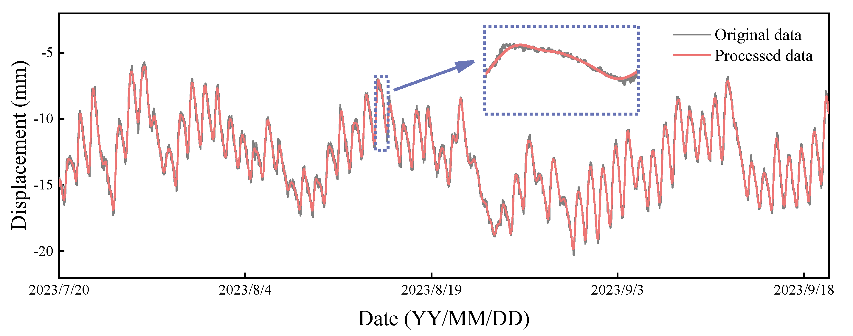
This study collects the measured data from the laser displacement meter DIS-03 and the vibrating string strain gauge RSG-03 to conduct follow-up research. The collection time of bearing displacement is from 20 July 2023 to 19 September 2023, and the collection time of strain is from 15 October 2023 to 15 December 2023, with a data collection interval of 10 min. Using the measurement data from the laser displacement meter DIS-03 for illustrative purposes, Figure 8 and Figure 9 illustrates the curve of bearing displacement over time. Notably, the data collected in this paper contains no missing values or outliers. Each response dataset therefore covers an observation period of approximately two months rather than a complete annual monitoring cycle. Consequently, the present data do not capture the full range of seasonal variability or longer-term structural and environmental evolution.
Figure 8.
The raw data from the laser displacement meter DIS-03.
The archived monitoring records available for this study do not contain documented sensor-failure-induced missing intervals. Therefore, controlled masking of complete measured sequences was adopted to construct consecutive missing-data cases. This strategy allows the original measurements within the masked intervals to serve as ground truth for quantitative evaluation. It should be emphasized that the purpose of this procedure is not to reproduce all possible sensor failure mechanisms, but to evaluate the proposed model under controlled consecutive data-interruption scenarios.
To avoid information leakage, the Savitzky-Golay filtering was performed only after chronological data partitioning and was never applied across the development/test boundary. During test-time recovery, for each consecutive missing interval beginning after time , the filtering operation was restricted to the observations available up to . No sample belonging to the masked interval was included in the filtering window or otherwise used during preprocessing. Thus, although the Savitzky-Golay filter uses neighboring observations within the available historical sequence, it does not access future target values beyond the forecast origin.
The preprocessing procedure was performed in a fixed sequence. First, the completeness and quality of the monitoring records were checked. No missing observations or abnormal outliers were identified in either the bearing-displacement or strain records used in this study; therefore, no outlier-removal or replacement operation was applied. Second, the bearing-displacement record was denoised using a Savitzky-Golay filter with a third-order polynomial and a window length of 11 samples. Considering the 10 min sampling interval, the smoothing window corresponds to 110 min. No additional denoising operation was applied to the strain record. Third, the monitoring data were normalized before model training and prediction using min-max normalization. For each response quantity, the minimum and maximum values used for normalization were determined from the model-development dataset and were subsequently fixed when transforming the validation and test data. The normalization is expressed as where and denote the minimum and maximum values of the corresponding response in the model-development dataset. After prediction, the reconstructed values were transformed back to their original physical units using
The inverse-transformed displacement and strain sequences were then used to calculate all reported evaluation metrics.
Figure 9.
Comparison between the original bearing displacement curve and the curve after noise reduction.
2.3. Model Preparation
The bearing-displacement sequence was first divided chronologically into a model-development dataset and an independent test dataset. The preprocessing operations described in Section 2.2 were then applied within the corresponding data partitions without crossing the partition boundary. The first 70% of the sequence, containing 6250 samples, was used for model development, whereas the remaining 30%, containing 2679 samples, was retained exclusively for final testing. The test dataset was not used for hyperparameter selection or model checkpoint selection.
For hyperparameter tuning, the 6250-sample development dataset was further divided chronologically into an internal training subset and a validation subset at a ratio of 80:20. Accordingly, the first 5000 samples were used for parameter optimization and the subsequent 1250 samples were used for validation. After the hyperparameters had been determined, the model was retrained using the complete 6250-sample development dataset and subsequently evaluated once on the untouched 2679-sample test dataset. This chronological hold-out strategy was adopted instead of random splitting in order to avoid disrupting the temporal dependence of the bridge-monitoring sequence.
Hyperparameter selection was performed using a structured two-stage coarse-to-fine search rather than relying solely on an unconstrained trial-and-error procedure. In the first stage, architecture-related parameters, including the number and hidden dimensions of the LSTM layers, Informer sequence length, decoder label length, encoder/decoder depth, model dimension, feed-forward dimension, and number of attention heads, were screened within predefined candidate ranges. In the second stage, training-related parameters, including the learning rate, batch size, optimizer, and maximum number of training epochs, were examined while the architecture selected in the first stage was retained.
Candidate configurations were evaluated using the chronologically separated validation subset. Because the same architecture was subsequently employed for different missing-data lengths, the parameter configuration was selected according to its overall validation behavior rather than being separately optimized for each prediction horizon. Representative short-, medium-, and long-horizon tasks (pred_len = 1, 24, and 72) were considered during parameter screening, and the configuration showing the most stable overall validation performance was retained. Except for pred_len, the same final hyperparameter configuration was subsequently used for the six recovery horizons of 1, 12, 24, 36, 48, and 72 points. The candidate ranges and selected values are summarized in Table 2.
Table 2.
Values of main hyperparameters in the LSTM-Informer model.
The sequence-length parameters of the Informer were further examined considering the temporal resolution of the monitoring data. Since the sampling interval is 10 min, the encoder input length of 30 corresponds to a 5 h historical observation window. The decoder label length of 15 corresponds to 2.5 h of known historical context supplied to the generative decoder and should not be confused with the prediction horizon, which is independently controlled by pred_len. The selection of seq_len = 30 and label_len = 15 is not intended to imply a unique physical periodicity of the bridge response. Instead, these values were determined by balancing the amount of historical information available to the model against the additional computational and modeling complexity associated with longer input sequences. A sensitivity analysis of these two parameters is provided in Section 3.4.
Based on the above validation procedure, the final learning rate was set to , the batch size was 32, and Adam was adopted as the optimizer. MSE was used as the training loss function. Each candidate model was trained for a maximum of 50 epochs, and the checkpoint corresponding to the lowest validation MSE was retained. Importantly, model selection was based exclusively on the internal validation subset rather than on the independent test dataset. After the final hyperparameter configuration was determined, the model was retrained using the complete 6250-sample development dataset before evaluation on the 2679-sample test sequence.
No Bayesian optimization, particle swarm optimization, or conventional random -fold cross-validation was employed in this study. Because the monitoring observations form a temporally ordered sequence, random cross-validation could disrupt temporal dependence and permit future observations to enter training folds preceding earlier validation observations. A chronological hold-out validation strategy was therefore adopted. Bayesian optimization and other automated search strategies may provide a more efficient exploration of larger hyperparameter spaces and will be investigated in future work.
The experimental platform consisted of Windows 11, MATLAB R2023b for ICEEMDAN-PE processing, and Python 3.9 with PyTorch for neural-network training and inference. The computations were performed using an AMD Ryzen 7 7735H CPU and an NVIDIA GeForce RTX 4060 Laptop GPU( Lenovo, Beijing, China).
The missing-data simulation adopted in this study follows a controlled block-masking protocol. First, the measured sequence is chronologically divided into training and test sets at a ratio of 70% and 30%, respectively. Second, model training is performed using the available training sequence. Third, consecutive blocks in the test sequence are treated as unavailable measurements, with block lengths of 1, 12, 24, 36, 48, and 72 samples. For the 10 min sampling interval used in the Badahe Bridge SHM system, these block lengths correspond to missing durations ranging from 10 min to 12 h.
For each missing-data length, the evaluation was not based on a single artificially selected missing segment. Instead, the test sequence was traversed using a sliding window whose step size was equal to the prediction horizon. Consequently, multiple non-overlapping target blocks distributed throughout the test period were evaluated for each horizon. The performance metrics reported in this study were calculated by aggregating predictions over all eligible test windows for the corresponding horizon, rather than from a single selected gap. This procedure exposes the models to missing intervals occurring at different temporal locations and response states within the test sequence.
These missing lengths were selected as controlled benchmark horizons rather than being derived from an empirical distribution of sensor-failure durations in the Badahe Bridge SHM system. The one-step case represents the shortest possible single-record loss, while the 12-, 24-, 36-, and 48-step cases provide progressively increasing 2 h increments, and the 72-step case extends the evaluation to a 12 h interruption. This design was intended to examine how reconstruction accuracy changes from short to relatively long consecutive gaps under a consistent experimental protocol. Because the archived records available for this study do not contain documented sensor-failure events with reliable duration labels, the considered 2–12 h outages should not be interpreted as an empirically established failure-duration distribution for the investigated SHM system.
Finally, the model-reconstructed values are compared with the originally measured values retained as ground truth using MSE, RMSE, MAE, MAPE, and R2. This protocol is designed specifically for consecutive measurement interruptions and is not intended to represent irregular pointwise missingness or corrupted sensor measurements.
The artificial missing segments were generated systematically from the independent test sequence rather than being manually selected. For each prediction horizon , each recovery sample consisted of a 30-sample observed historical window followed immediately by an -sample target block that was treated as consecutively missing. During testing, the starting position of successive windows was advanced by samples; therefore, the target missing blocks did not overlap. Each test window was treated as an independent recovery case. After one target block had been evaluated, the next input window was constructed from the original measured test sequence. Therefore, the true measurements belonging to the preceding target block could appear as historical inputs in the subsequent test window. The predicted values from one block were not recursively fed into the next block. Consequently, the present experiment evaluates multiple independent consecutive missing intervals of a prescribed length \( H\) , rather than a single continuously expanding missing interval. For a test sequence containing 2679 samples, the number of complete recovery blocks was calculated as
Accordingly, 2649, 220, 110, 73, 55, and 36 missing segments were evaluated for prediction horizons of 1, 12, 24, 36, 48, and 72 samples, respectively. Any residual samples at the end of the test sequence that were insufficient to form a complete input–target pair were excluded. Thus, no missing interval was manually selected according to prediction performance. For , the evaluation uses all regularly generated non-overlapping target blocks with a stride of , rather than every possible overlapping window.
The missing-data simulation adopted in this study is specifically designed for consecutive measurement interruptions that can be formulated as forward multi-step prediction from the observations available immediately before the interruption. Therefore, the framework is directly applicable to terminal consecutive missing sequences, such as temporary acquisition or communication outages for which the most recent measurements are available but the subsequent observations are temporarily unavailable. An internal consecutive missing interval can also be treated in a forward-prediction manner using the observations preceding the gap; however, the present framework does not exploit observations available after the missing interval and should therefore not be interpreted as a bidirectional interpolation method. Irregularly distributed or intermittent pointwise missing values were not specifically considered in this study. Although the one-step case represents the limiting case of a single consecutive missing observation, it does not constitute validation for general intermittent missingness.
2.4. Prediction Model
To evaluate the proposed model’s effectiveness and robustness, we selected several comparison models, including LSTM, CNN-LSTM, Informer, LSTM-Informer, and CEEMDAN-PE-LSTM-Informer, to compare with the ICEEMDAN-PE-LSTM-Informer model. A comprehensive summary of all the models involved in this study is provided in Table 3. It is important to note that both the LSTM and CNN-LSTM models employ a direct output prediction strategy, meaning that all predicted values are generated simultaneously. Moreover, the CNN-LSTM model initially extracts features from the input sequence through 1D convolution, subsequently feeding these extracted features into the LSTM model for prediction. Owing to its unique and effective structural design, this model has been widely adopted across the specialized domain of bridge engineering [47,48,49,50]. It is worth noting that the experimental environment used by the above comparison model is consistent with that of the ICEEMDAN-PE-LSTM-Informer model.
Table 3.
Comparison models and their roles in the experimental design.
The comparison models were selected according to a controlled, component-oriented strategy rather than with the intention of constructing an exhaustive benchmark of all available time-series architectures. Each baseline was included to answer a specific methodological question related to the proposed framework. LSTM was selected as the recurrent baseline because it constitutes one branch of the proposed architecture and is widely used for temporal prediction and missing-data reconstruction in SHM. Informer was selected as the attention-based baseline because it constitutes the second branch of the proposed framework and is specifically designed for efficient long-sequence forecasting. Their direct comparison therefore clarifies the respective behavior of recurrent and attention-based temporal modeling.
LSTM-Informer was included to evaluate whether combining the two prediction mechanisms improves reconstruction relative to the corresponding single-branch models. CNN-LSTM was selected as a representative convolution–recurrent hybrid architecture that has been applied to nonlinear bridge-monitoring response prediction, thereby providing a structurally different deep-learning baseline. CEEMDAN-PE-LSTM-Informer was included for a different purpose: because ICEEMDAN is developed from the CEEMDAN family, replacing only ICEEMDAN with CEEMDAN while retaining PE regrouping and the same LSTM-Informer predictor enables a relatively controlled evaluation of the contribution of the decomposition strategy. Finally, comparison between the complete model and LSTM-Informer without decomposition provides an assessment of the overall contribution of the signal decomposition and regrouping stage.
Accordingly, the selected baselines cover four aspects of the proposed method: (1) recurrent temporal modeling (LSTM); (2) attention-based long-range modeling (Informer); (3) hybrid temporal-feature extraction (CNN-LSTM and LSTM-Informer); and (4) decomposition-assisted prediction (CEEMDAN-PE-LSTM-Informer). This design allows the principal architectural choices in the proposed framework to be examined under the same data partition, prediction horizons, training protocol, and evaluation metrics.
For fairness, all prediction models used exactly the same chronological development/test partition and the same artificial missing-data windows for each prediction horizon. Hyperparameter selection for each baseline was performed independently using the same internal chronological training/validation split described in Section 2.3, without access to the independent test set. Model-specific architectural parameters were tuned within predefined candidate ranges appropriate to each architecture, whereas the optimization protocol was kept comparable across models. In particular, all models used MSE as the optimization objective, Adam as the optimizer, a batch size of 32, a maximum training budget of 50 epochs per candidate configuration, and validation MSE for checkpoint selection. Thus, the comparison used a common validation and training budget rather than selecting baseline settings according to test-set performance. Because the architectures differ in parameter count and computational complexity, identical wall-clock training times were neither expected nor enforced.
Other representative methods, including Transformer, GRU, TCN, GAN-based reconstruction, VMD-based hybrid models, and TVFEMD-based approaches, were also considered when defining the benchmark scope. However, they were not all included as numerical baselines because the objective of the present comparison is to isolate the main design choices of the proposed framework under a unified experimental protocol. A conventional Transformer was not separately included because Informer is a Transformer-derived architecture and is the attention-based branch directly employed in the proposed model; including Informer therefore provides a more direct controlled comparison for the present architecture. Similarly, GRU belongs to the same recurrent-gated modeling family as LSTM, whereas LSTM was selected because it is the recurrent branch actually used in the proposed framework. TCN represents another valuable temporal-convolutional architecture, but CNN-LSTM was retained as the convolution–recurrent baseline in order to limit the number of architectures while maintaining a structurally different comparison model.
GAN-based methods formulate missing-data reconstruction as a generative-learning problem and generally require a different training objective and data-generation strategy from the direct multi-step forecasting framework adopted here. Therefore, a numerical GAN comparison would not constitute a strict one-component-at-a-time comparison under the present prediction protocol. With respect to signal decomposition, VMD and TVFEMD represent important alternatives to EMD-family methods and have been combined with subsequent intelligent-analysis models in different structural and time-series applications. For example, Wu et al. [51] incorporated VMD into an array-ultrasonic inspection framework to suppress signal noise before SAFT imaging, followed by deep-learning-based identification of internal concrete defects. This study illustrates the usefulness of VMD as a signal-preprocessing tool for enhancing subsequent feature extraction and intelligent structural-condition assessment. Nevertheless, CEEMDAN was retained as the primary numerical decomposition baseline in the present study because it is methodologically more directly related to ICEEMDAN, thereby allowing the decomposition strategy to be changed while PE regrouping and the downstream LSTM-Informer architecture remain unchanged. Thus, Model 1 versus Model 2 provides a more controlled decomposition comparison than replacing the entire preprocessing framework with a method requiring different decomposition parameters and component structures.
The omission of these methods from the numerical benchmark should therefore not be interpreted as indicating that they are inferior. Rather, the present comparison was designed to prioritize controlled attribution of performance differences to the principal components of the proposed framework. Broader benchmarking against additional recurrent, convolutional, generative, and decomposition-based architectures remains valuable for future cross-model evaluation.
To further isolate the contribution of the main components of the proposed framework, three additional ablation variants were constructed. In the first variant, PE-based regrouping was removed while ICEEMDAN decomposition and the LSTM–Informer prediction architecture were retained. In the second and third variants, the Informer and LSTM branches were removed separately while the ICEEMDAN-PE preprocessing procedure remained unchanged. Together with the existing CEEMDAN-PE-LSTM-Informer and LSTM-Informer models, these variants enable the effects of the decomposition strategy, PE-based regrouping, and parallel neural-network architecture to be assessed individually. The corresponding results are presented in Section 3.3.
2.5. Model Evaluation Metrics
To conduct a more comprehensive evaluation of the predictive capability of the proposed model, a suite of commonly adopted error assessment metrics was introduced, including mean squared error (MSE), root mean square error (RMSE), mean absolute error (MAE), mean absolute percentage error (MAPE), and the coefficient of determination (R2). Lower numerical values of MSE, RMSE, MAE and MAPE are indicative of superior accuracy in the generated prediction outcomes. In contrast, a value of (R2) that approaches 1 more closely signifies more favorable predictive performance of the model. The mathematical formulas for calculating the above-mentioned error assessment metrics are presented as follows:
All evaluation metrics in this study are calculated after the predicted sequences have been transformed back from the normalized scale to their original physical scale. Therefore, for bearing displacement, RMSE and MAE are expressed in millimeters (mm), while MSE is expressed in mm2. For the strain dataset, RMSE and MAE are expressed in microstrain (με), and MSE is expressed in (με)2. is dimensionless, whereas MAPE is reported as a percentage. This evaluation procedure ensures that the reported errors can be directly interpreted in terms of the measured structural responses rather than in normalized units.
MAPE is calculated as
where and denote the measured and reconstructed values in the original physical units, respectively. The absolute value is applied to the relative error; therefore, negative displacement or strain values do not themselves cause a sign problem. However, MAPE becomes unstable when the measured value approaches zero. In the two monitoring datasets considered in this study, the evaluated displacement and strain sequences remain sufficiently separated from zero, and no zero-valued observations occur in the evaluated intervals. Nevertheless, because of this inherent limitation, MAPE is used only as a supplementary relative-error indicator, while RMSE, MAE, and are emphasized in the interpretation of model performance.
3. Results and Discussion
3.1. Data Set Preparation
Take the recovery of the missing bearing displacement data in the Badahe Bridge’s SHM system as an example. Initially, the bearing displacement was proportionally divided into the training and test data sets (refer to Section 2.3). Subsequently, the ICEEMDAN technology was used to decompose each of these data sets separately. Among them, the training dataset was divided into 12 modal components, while the test dataset was divided into 10 modal components, as shown in Figure 10a,b. The decomposition results indicate that the decomposed subsequences exhibit greater regularity compared to the original sequences, effectively capturing the characteristics of the sequences across different time scales.
Figure 10.
The IMFs obtained by ICEEMDAN decomposition.
In addition, the normalized permutation entropy (PE) of each IMF was calculated using an embedding dimension of and a delay time of . It should be noted that PE was not used to directly determine the frequency of an IMF. The IMFs obtained by ICEEMDAN are inherently arranged from relatively high-frequency/short-scale components to low-frequency/long-scale components, whereas PE was employed to quantify their temporal complexity and to determine the regrouping boundaries.
Specifically, the difference in normalized PE between two adjacent IMFs was calculated as where denotes the normalized PE of the -th IMF. The two largest adjacent PE differences were selected as the regrouping boundaries. The same PE parameters and regrouping criterion were applied independently to both the training and test datasets, without introducing dataset-specific fixed thresholds. The calculated PE values and resulting group assignments are summarized in Table 4.
Table 4.
Normalized permutation entropy of the ICEEMDAN components.
For the training dataset, the two most pronounced changes in PE occurred between IMF4–IMF5 and IMF7–IMF8. Therefore, IMF1–4, IMF5–7, and IMF8–12 were reconstructed as , , and , respectively. The same grouping boundaries were identified for the test dataset, resulting in IMF1–4, IMF5–7, and IMF8–10 being reconstructed as , , and , respectively. Although the training and test datasets contained different numbers of IMFs, the same PE calculation parameters and grouping criterion were used.
As shown in Table 3, the normalized PE generally decreases with increasing IMF order, reflecting a gradual transition from highly irregular short-scale components to more regular long-scale components. For the training dataset, the two largest adjacent PE differences are observed between IMF4–IMF5 () and IMF7–IMF8 (). Accordingly, these positions are selected as the two regrouping boundaries. A similar PE distribution is observed for the test dataset, where the corresponding adjacent differences are 0.147 and 0.216. Therefore, despite the different total numbers of IMFs obtained from the training and test datasets, the same data-adaptive grouping criterion produces consistent boundaries at IMF4–IMF5 and IMF7–IMF8.
Table 5 further illustrates the consistency of the reconstructed components despite the different numbers of original IMFs. ICEEMDAN produces 12 IMFs from the 6250-point training sequence and 10 IMFs from the 2679-point test sequence. After applying the same PE-based regrouping criterion, however, both datasets are represented by exactly three reconstructed components. The mean normalized PE values of the high-, medium-, and low-frequency groups are 0.9005, 0.6803, and 0.3532 for the training dataset and 0.9043, 0.6907, and 0.4050 for the test dataset, respectively. Thus, the three reconstructed groups preserve the same descending complexity hierarchy in both datasets despite the different numbers of constituent IMFs.
Table 5.
Consistency of PE-based component reconstruction between the training and test datasets.
This result indicates that correspondence between the training and test data is established at the reconstructed-component level rather than through one-to-one matching of individual IMFs. Consequently, the high-, medium-, and low-frequency predictors trained on the training dataset retain the same functional correspondence when applied to the independently decomposed test dataset. The reconstructed components are shown in Figure 11.
Figure 11.
The result of frequency division recombination of two data sets.
3.2. Example of the Data Recovery
This study specifically focuses on consecutive missing measurements caused by temporary interruption of data acquisition or transmission. The recovery task is formulated as forward multi-step prediction: the observations available immediately before an interruption are used to reconstruct the subsequent unavailable sequence. This formulation directly represents terminal missing sequences during an ongoing interruption and can also be applied to an internal consecutive gap by forecasting forward from its left boundary. In the latter case, measurements available after the gap are not used by the present model. Therefore, the experiments should be interpreted as evaluating unidirectional consecutive-gap recovery rather than general bidirectional interpolation or irregular/intermittent missing-data imputation. Six missing-data lengths, namely 1, 12, 24, 36, 48, and 72 consecutive samples, were considered. Given the 10 min sampling interval of the SHM system, these cases correspond to interruption durations of 10 min, 2 h, 4 h, 6 h, 8 h, and 12 h, respectively. Therefore, the present evaluation covers consecutive data interruptions from short gaps to relatively long-duration outages, rather than all possible forms of sensor failure. Here, each missing interval is evaluated independently; therefore, the 72-step case represents direct reconstruction of an individual 12 h consecutive gap and should not be interpreted as recursive recovery of a continuously expanding outage beyond 12 h.
Under each operational condition, the decomposed and reorganized components described in Section 3.1 were subjected to individual predictive analysis using the proposed LSTM-Informer model. Prediction results derived from each component were then combined via linear superposition to generate the overall forecasting outcomes. In addition, to validate the effectiveness of the model proposed herein, the comparison models constructed in Section 2.4 (Models 2~6) were juxtaposed against the core model of this study (Model 1). The evaluation metrics for each model under different forecast time steps are tabulated in Table 6. To streamline the presentation, Figure 12, Figure 13, Figure 14 and Figure 15 present the results for prediction horizons of 1, 24, 48, and 72 steps, corresponding to consecutive missing-data durations of 10 min, 4 h, 8 h, and 12 h, respectively.
Table 6.
Evaluation metrics of Models 1–6 under consecutive missing-data durations ranging from 10 min (1 step) to 12 h (72 steps).
Figure 12.
Reconstruction results for a 1-step (10 min) consecutive missing interval.
Figure 13.
Reconstruction results for a 24-step (4 h) consecutive missing interval.
Figure 14.
Reconstruction results for a 48-step (8 h) consecutive missing interval.
Figure 15.
Reconstruction results for a 72-step (12 h) consecutive missing interval.
As shown in Figure 12, when the predicted time step is set to 1, all models perform better, with the predicted curve nearly overlapping the actual curve. However, as the time step increases (Figure 13, Figure 14 and Figure 15), Model 1 exhibits superior accuracy in predicting bearing displacement compared to the other models. It shows a better overall fitting effect, aligning more closely with the true values, and possesses a stronger capacity to capture both long-term and local dependence relationships. Especially for the peak and trough positions of the actual curve, the prediction error of Model 1 is notably smaller when compared against the true values. However, for other models, such as Model 6, when the time step is long, the divergence between the predicted curve and the measured curve is found to be substantial, especially at the peaks and troughs of the curve.
By analyzing the error values of each model in Table 5 under different predicted time steps, the following observations can be summarized:
- (a)
- By comparing the recovery performance of Model 4 and Model 6 across various predicted time steps, we observe that LSTM excels in short-term predictions. In contrast, Informer demonstrates superior performance in long-term predictions. Specifically, when the predicted time step is set to 1, LSTM outperforms Informer, reducing the RMSE by 60.24% compared to Informer. However, Informer demonstrates superior performance over LSTM at time steps 12, 24, 36, 48, and 72, with RMSE reductions of 10.22%, 10.50%, 15.74%, 13.49%, and 14.83%, respectively. The results show that LSTM performs better than Informer at the one-step horizon, whereas Informer achieves lower RMSE values than LSTM for the longer prediction horizons considered in this study. One possible explanation is related to the different architectural characteristics of the two models. LSTM employs recurrent gating to propagate temporal information sequentially, whereas Informer uses a ProbSparse self-attention mechanism designed to model dependencies over longer sequences more efficiently. These architectural differences are consistent with the observed horizon-dependent performance. However, the present experiments do not directly examine gradient propagation, attention distributions, or internal feature representations, and therefore the performance differences should not be interpreted as direct evidence that gradient attenuation or ProbSparse attention is the specific causal mechanism responsible for the observed results.
- (b)
- By comparing the recovery performance of Models 3, 4, 5, and 6 across different predicted time steps, it is readily apparent that the LSTM-Informer model exhibits superior performance over the other comparative models across the majority of test scenarios. For example, when the predicted time steps are 1, 12, 24, 36, 48, and 72, the RMSE of LSTM-Informer decreases by 18.91%, 40.55%, 21.66%, 18.05%, 24.05%, and 19.11% compared to LSTM. Compared to Informer, the RMSE decreases by 67.75%, 33.78%, 12.47%, 2.74%, 12.20%, and 5.02%. This shows that the parallel combination of LSTM and Informer is practical. Moreover, the performance of CNN-LSTM surpasses that of LSTM-Informer when the predicted time step is set to 1, with its RMSE being 19.94% lower than that of LSTM-Informer. However, for time steps 12, 24, 36, 48, and 72, the prediction accuracy of CNN-LSTM is inferior to that of LSTM-Informer. Specifically, the RMSE of LSTM-Informer is 6.81%, 18.16%, 15.19%, 15.60%, and 12.02% lower than that of CNN-LSTM, respectively. The outcomes of the analysis reveal that the CNN-LSTM model yields enhanced predictive performance when contrasted with the standalone LSTM model; however, its overall predictive effectiveness and applicability do not surpass those of the LSTM-Informer. Therefore, the LSTM-Informer is the most suitable model architecture, as it is more effective in recovering missing data within the SHM system.
- (c)
- In most cases, the recovery performance of all hybrid models surpasses that of their single-model counterparts across varying prediction time steps. For instance, for a predicted time step of 72, the RMSE of ICEEMDAN-PE-LSTM-Informer is 54.06%, 50.14%, 46.06%, and 43.21% lower than that of LSTM, CNN-LSTM, Informer, and LSTM-Informer, respectively. Similarly, the RMSE of CEEMDAN-PE-LSTM-Informer is 19.49%, 12.61%, 5.47%, and 0.47% lower than that of LSTM, CNN-LSTM, Informer, and LSTM-Informer, respectively. The root reason for this phenomenon lies in the distinctive functionality of decomposition technology within the mixed model to effectively capture the diverse features present in the sequence, thereby mitigating the interference of nonlinear components from the original sequence on model predictions. Consequently, introducing decomposition technology during the data preprocessing stage can significantly enhance the effectiveness of missing data recovery.
- (d)
- In hybrid modeling frameworks, the LSTM-Informer model integrated with ICEEMDAN decomposition demonstrates superior predictive performance compared to its counterpart combined with CEEMDAN decomposition. For example, for a predicted time step of 72, the RMSE, MSE, MAE, and MAPE of ICEEMDAN-PE-LSTM-Informer are 42.94%, 67.45%, 47.08%, and 46.92% lower than those of CEEMDAN-PE-LSTM-Informer, respectively. Additionally, the R2 is 11.73% higher than that of CEEMDAN-PE-LSTM-Informer. This is because although CEEMDAN represents an advancement over EMD and EEMD, it remains susceptible to mode aliasing issues. By incorporating adaptive noise and enhancing noise processing techniques, ICEEMDAN can more effectively mitigate mode aliasing and produce a more consistent multiscale decomposition and reduce residual mode-mixing effects. Thus, the ICEEMDAN-PE-LSTM-Informer hybrid model can efficiently tackle the technical challenge associated with missing data restoration during the structural health monitoring (SHM) of bridge structures.
- (e)
- As the length of the prediction time step expands, the predictive precision of every individual model tends to decline gradually. Specifically, for predicted time steps 12, 24, 36, 48, and 72, the RMSE of ICEEMDAN-PE-LSTM-Informer increases by 0.057, 0.1615, 0.2455, 0.4242, and 0.4959, respectively, compared to the RMSE at a predicted time step of 1. Similarly, the RMSE of LSTM rises by 0.1724, 0.3208, 0.4148, 0.6106, and 1.0785 when compared to the RMSE at a predicted time step of 1. This finding aligns with the conclusions of Xin et al. [15] and Hao et al. [34] regarding missing data prediction in the SHM of bridges. Furthermore, as the prediction horizon increases, the reconstruction error of the LSTM model rises more rapidly than that of the proposed model. Under the investigated prediction horizons, the ICEEMDAN-PE-LSTM-Informer framework exhibits a comparatively slower degradation in reconstruction accuracy. This result indicates relatively favorable horizon-dependent performance, but it should not be interpreted as a comprehensive robustness assessment because explicit perturbation tests were not conducted in the present study. This observation reflects its relative stability across the investigated prediction horizons, rather than statistical robustness with respect to different random initializations.
From an engineering perspective, the reported errors are expressed directly in displacement units after inverse normalization. For example, for the most challenging 72-step case, corresponding to a 12 h consecutive missing interval, the proposed model yields an RMSE of 0.5156 mm and an MAE of 0.3578 mm. Thus, the characteristic reconstruction error remains at the sub-millimeter level, while the mean absolute deviation between reconstructed and measured bearing displacement is approximately 0.36 mm. This physical-unit interpretation is more informative for engineering assessment than the normalized prediction error alone.
RMSE assigns greater weight to relatively large local deviations and is therefore useful for identifying deterioration in the reconstruction of peaks and troughs, whereas MAE directly represents the average absolute discrepancy between reconstructed and measured responses in physical units.
3.3. Ablation Study
To further quantify the independent contributions of the major components in the proposed ICEEMDAN-PE-LSTM-Informer framework, an ablation study was conducted based on the bearing displacement dataset. Unlike the general benchmark comparisons presented in Section 3.2, the present analysis modifies one principal component at a time while retaining the remaining parts of the framework as consistently as possible. In this way, the effects of the decomposition strategy, PE-based regrouping, and the parallel LSTM-Informer architecture can be examined separately.
Six model configurations were considered. A0 denotes the complete ICEEMDAN-PE-LSTM-Informer model. In A1, ICEEMDAN was replaced by CEEMDAN, while the subsequent PE regrouping and LSTM-Informer prediction architecture remained unchanged. This configuration corresponds to the CEEMDAN-PE-LSTM-Informer model already considered in Section 3.2 and is used to evaluate the influence of the decomposition strategy. In A2, the PE-guided regrouping procedure was removed. Specifically, the IMFs generated by ICEEMDAN were retained in their intrinsic high-to-low frequency order and divided into three approximately equal groups according to their IMF indices, without calculating permutation entropy. This fixed grouping preserves the same three-component prediction structure as the complete model, thereby allowing the effect of PE-guided regrouping to be evaluated without changing the number of prediction branches. In A3, the Informer branch was removed and the ICEEMDAN-PE components were predicted only by the LSTM network. Conversely, in A4, the LSTM branch was removed and only the Informer network was retained. Finally, A5 corresponds to the LSTM-Informer model without ICEEMDAN decomposition and PE regrouping, and therefore provides an additional reference for evaluating the overall contribution of the decomposition-and-regrouping preprocessing stage.
The RMSE results obtained for the six configurations under prediction horizons of 1, 12, 24, 36, 48, and 72 steps, corresponding to missing-data durations of 10 min, 2 h, 4 h, 6 h, 8 h, and 12 h, respectively are summarized in Table 7. Overall, the complete model maintains the lowest reconstruction error across the investigated prediction horizons. However, the performance degradation caused by removing or replacing individual components is not uniform with increasing prediction length, indicating that the different modules play complementary rather than identical roles in the reconstruction process.
Table 7.
RMSE results of the ablation study under different prediction horizons and corresponding consecutive missing-data durations.
First, the comparison between A0 and A1 isolates the influence of the decomposition method because the PE regrouping strategy and the subsequent LSTM-Informer architecture are identical in the two models. At the 72-step prediction horizon, replacing ICEEMDAN with CEEMDAN increases the RMSE from 0.5156 to 0.9036. Equivalently, the use of ICEEMDAN reduces the RMSE by 42.94% relative to the CEEMDAN-based configuration. The difference is smaller at some intermediate horizons, such as the 48-step case, indicating that the advantage of ICEEMDAN is dependent on the prediction horizon rather than being uniformly large under all conditions. Nevertheless, the overall results suggest that the improved decomposition strategy contributes to reducing reconstruction error, particularly for relatively long missing intervals. This observation is consistent with the design objective of ICEEMDAN, which seeks to alleviate residual noise and spurious modal components during signal decomposition. Because the present comparison is based primarily on downstream reconstruction performance, the decomposition-level mechanism itself is not independently established here.
Second, comparison between A0 and A2 demonstrates the contribution of PE-based regrouping. When PE-guided regrouping is replaced by the fixed IMF-index grouping strategy, the RMSE increases from 0.5156 to 0.5984 at the 72-step prediction horizon, corresponding to an RMSE reduction of approximately 13.84% after PE-based regrouping is introduced. Similar but relatively moderate improvements can also be observed at the shorter prediction horizons. These results indicate that the role of PE is mainly to provide a more appropriate organization of decomposed components according to their temporal complexity, rather than to directly perform prediction. By grouping IMFs with similar complexity characteristics, PE reduces the heterogeneity within each reconstructed component and provides more structured inputs for the subsequent prediction networks.
Third, A3 and A4 were used to assess the individual roles of the Informer and LSTM branches within the parallel prediction architecture. At the one-step horizon, removing the Informer branch only increases the RMSE from 0.0197 to 0.0210, whereas removing the LSTM branch increases it to 0.0325. This result indicates that the LSTM branch makes a particularly important contribution to short-horizon reconstruction. In contrast, as the prediction horizon increases, the effect of the Informer branch becomes increasingly evident. At the 72-step horizon, the RMSE values of the models without the Informer and LSTM branches are 0.7423 and 0.6649, respectively, compared with 0.5156 for the complete model. Relative to the corresponding single-branch variants, the complete parallel architecture reduces RMSE by approximately 30.54% and 22.45%, respectively. This horizon-dependent behavior is consistent with the intended complementary roles of the two branches. The recurrent LSTM branch is designed to model local and relatively short-term temporal dependencies, whereas the Informer branch incorporates ProbSparse self-attention for efficient long-range dependency modeling. The present ablation results support the usefulness of retaining both branches, but they do not directly identify the internal mechanism responsible for the observed performance differences.
The role of the complete decomposition-and-regrouping stage can also be observed by comparing A0 with A5. At the 72-step horizon, the RMSE decreases from 0.9079 for the LSTM-Informer model without decomposition to 0.5156 for the complete model, corresponding to a reduction of 43.21%. This result indicates that the improvement of the proposed framework cannot be attributed solely to the neural-network architecture. The decomposition and regrouping procedure substantially reduces the modeling difficulty associated with the nonlinear and non-stationary characteristics of the original monitoring sequence before temporal prediction is performed.
Taken together, the ablation results demonstrate that the performance improvement of the proposed framework arises from the combined effects of several complementary components rather than from a single processing stage. ICEEMDAN improves the representation of the original non-stationary signal, PE provides an adaptive criterion for reorganizing decomposed components, and the parallel LSTM-Informer architecture combines local temporal modeling with long-range dependency extraction. Importantly, the magnitude of the performance degradation caused by each ablation varies with the prediction horizon. Therefore, the present results should not be interpreted as assigning a fixed relative importance to each component; instead, they demonstrate that all three design choices make measurable contributions to the reconstruction performance under the investigated consecutive missing-data conditions.
3.4. Sensitivity Analysis of Sequence-Length Parameters
The input sequence length and decoder label length determine the amount of historical information supplied to the Informer and therefore may influence the reconstruction performance. Considering the 10 min sampling interval of the bridge SHM system, the adopted encoder sequence length of 30 corresponds to a 5 h historical observation window, while the decoder label length of 15 provides 2.5 h of known historical context before generation of the prediction sequence. To examine whether these settings unduly affect the reported performance, a sensitivity analysis was conducted for seq_len and label_len.
The two parameters were varied independently while all other network settings, training procedures, and data partitions were kept unchanged. First, seq_len was set to 24, 30, 48, and 72, corresponding to historical windows of 4, 5, 8, and 12 h, respectively, while label_len was fixed at 15. Second, label_len was varied among 5, 10, 15, 20, and 25 while seq_len was fixed at 30. The 24-step (4 h) and 72-step (12 h) reconstruction tasks were selected to represent medium- and long-duration consecutive missing-data recovery, respectively. The corresponding RMSE values are summarized in Table 8 and Table 9.
Table 8.
Sensitivity of seq_len.
Table 9.
Sensitivity of label_len.
As shown in Table 8, increasing the encoder input length from 24 to 30 improves the reconstruction accuracy for both prediction horizons. For the 72-step case, the RMSE decreases from 0.5468 to 0.5156. However, further increasing the input window to 48 and 72 samples does not result in additional improvement; instead, the RMSE increases slightly to 0.5279 and 0.5524, respectively. A similar trend is observed for the 24-step prediction. These results indicate that simply increasing the amount of historical information does not necessarily improve reconstruction accuracy. A relatively short input may provide insufficient temporal context, whereas an excessively long sequence may introduce redundant or weakly relevant historical information and increase the modeling burden. Under the present dataset and network configuration, seq_len = 30 provides a favorable balance between temporal context and prediction accuracy.
The decoder label length exhibits a similar moderate sensitivity. Increasing label_len from 5 to 15 progressively reduces the RMSE, indicating that an adequate amount of recent historical information is beneficial for initializing the generative decoder. At the 72-step horizon, the lowest RMSE is obtained at label_len = 15. Further increasing the known decoder context to 20 or 25 samples does not produce a consistent additional improvement. Therefore, label_len = 15, which corresponds to one half of the encoder input length, was retained in the final model.
Overall, the sensitivity analysis indicates that the performance of the proposed model is not dependent on an arbitrarily selected single input-window setting. Although the reconstruction accuracy varies with the amount of historical context, the results exhibit a relatively stable region around the adopted configuration. Consequently, seq_len = 30 and label_len = 15 were selected for the subsequent experiments. It should be emphasized that these values represent empirically suitable settings for the monitoring datasets considered in this study rather than universal optimal parameters for all bridge SHM applications.
3.5. Computational Cost and Practical Applicability
In addition to reconstruction accuracy, computational cost is an important consideration for the practical deployment of data recovery methods in bridge structural health monitoring systems. The proposed ICEEMDAN-PE-LSTM-Informer framework contains both signal-processing and neural-network prediction stages and is therefore computationally more complex than a standalone forecasting model. To quantitatively examine this additional computational burden, the computational requirements of the proposed method and the benchmark models were evaluated in terms of the number of trainable parameters, serialized model size, training time, neural-network inference time, preprocessing time, end-to-end recovery time, and peak GPU memory consumption.
All neural-network models were evaluated under the same hardware and software environment described in Section 2.3. The training time was obtained from three independent runs and is reported as the mean ± standard deviation. For inference-time measurement, the models were first executed for 20 warm-up iterations to reduce initialization effects, after which 100 forward predictions were performed and the mean execution time was recorded. GPU synchronization was applied before and after timing to ensure that asynchronous CUDA operations did not bias the reported inference time. The serialized model size was measured from the stored model parameter files rather than estimated solely from the theoretical memory required by floating-point parameters.
From the perspective of theoretical computational complexity, the principal cost of an LSTM layer scales approximately as , where denotes the sequence length, is the input dimension, and denotes the hidden-state dimension. In contrast, the ProbSparse self-attention mechanism adopted by the Informer reduces the attention-related complexity from approximately for conventional self-attention to approximately . Since ICEEMDAN is based on iterative empirical mode decomposition and repeated noise-assisted sifting, its computational cost depends on the signal length, the number of realizations, and the convergence behavior of the sifting procedure, and therefore cannot be adequately characterized by a single fixed analytical expression. For this reason, the computational cost of ICEEMDAN-PE was evaluated experimentally in terms of actual execution time.
It should also be noted that the complete ICEEMDAN-PE-LSTM-Informer framework contains three independently trained LSTM-Informer predictors corresponding to the reconstructed high-, medium-, and low-frequency components. Therefore, the reported parameter number and model size of the complete model include all three component predictors. By contrast, ICEEMDAN and PE do not introduce trainable neural-network parameters, and their computational contribution is reflected separately through the preprocessing time. The total recovery latency can therefore be expressed as , where is the signal decomposition and regrouping time and denotes the forward-inference time of the three trained prediction networks.
As summarized in Table 10, the computational requirements increase progressively from the standalone prediction models to the complete hybrid framework. The standalone LSTM contains approximately 0.31 million trainable parameters and requires 2.74 ± 0.11 min for training, whereas the Informer contains approximately 0.96 million parameters and requires 4.39 ± 0.17 min. In comparison, the complete ICEEMDAN-PE-LSTM-Informer framework contains approximately 3.81 million trainable parameters and requires 18.96 ± 0.52 min for training. Thus, the parameter count of the complete framework is approximately 12.29 and 3.97 times those of the standalone LSTM and Informer, respectively, while its training time is approximately 6.92 and 4.32 times longer. The peak GPU memory consumption also increases from 612 MB for LSTM and 846 MB for Informer to 1308 MB for the complete framework, corresponding to approximately 2.14 and 1.55 times the memory requirements of the two single models, respectively.
Table 10.
Computational cost of different prediction models.
A similar increase is observed for neural-network inference. The mean inference times of LSTM and Informer are 0.34 ± 0.03 and 0.71 ± 0.05 ms per prediction sample, respectively, whereas the three component-specific LSTM-Informer predictors in the complete framework require approximately 3.10 ± 0.12 ms in total. Therefore, the neural-network inference cost of the proposed framework is approximately 9.12 times that of LSTM and 4.37 times that of Informer. These results confirm that the improved reconstruction accuracy of the proposed framework is accompanied by increased computational and memory requirements and should therefore be interpreted as an explicit accuracy–computation trade-off rather than as a computationally lighter alternative to the standalone models.
For practical deployment, however, model training and online data recovery should be distinguished. Model training can be performed offline after sufficient historical monitoring data have been collected and therefore does not directly determine the latency of an individual recovery operation. During deployment, the principal computational operations are ICEEMDAN-PE preprocessing and forward inference through the three trained component-specific prediction networks. As shown in Table 10, neural-network inference requires only approximately 3.10 ms, whereas ICEEMDAN-PE preprocessing requires approximately 5.37 s. Consequently, the total end-to-end recovery time is approximately 5.373 s, indicating that signal decomposition and regrouping, rather than deep-learning inference, dominate the online computational latency.
Under the monitoring configuration investigated in this study, the sampling interval is 10 min (600 s). The measured end-to-end recovery latency of 5.373 s therefore corresponds to only approximately 0.90% of one sampling interval and is about 112 times shorter than the interval between two consecutive measurements. From the perspective of computational latency, the proposed method can therefore complete a recovery operation well before the next scheduled measurement under the present low-frequency SHM configuration. Accordingly, the results support its computational feasibility for near-real-time data recovery in the monitoring scenario considered in this study.
Nevertheless, this conclusion should not be interpreted as demonstrating universal real-time applicability. In monitoring systems with substantially higher sampling frequencies, larger datasets, or more extensive sensor networks, the ICEEMDAN preprocessing stage may become a computational bottleneck. Future work should therefore investigate accelerated or incremental decomposition strategies, unified implementation of the preprocessing and prediction stages, parallel computation of the reconstructed components, and model compression to reduce recovery latency without substantially sacrificing reconstruction accuracy.
3.6. Evaluation on a Different Structural Response Dataset
To further examine whether the proposed framework can be applied to a structural-response type different from the bearing-displacement data used in the primary evaluation, the strain measurements from sensor RSG-03 of the same Badahe Bridge SHM system were used as an additional dataset. This evaluation is intended to assess the model across two different response types within the same monitored structure rather than to establish cross-bridge, cross-sensor, or cross-season generalization.
For ease of analysis, Figure 16 shows the recovery effect of the ICEEMDAN-PE-LSTM-Informer model under different predicted time steps. As illustrated in the figure, the model’s prediction error tends to increase gradually with the extension of the time step. However, in terms of predictive effectiveness, the model developed herein demonstrates a superior ability to precisely predict the fluctuation patterns reflected by the curve. Additionally, the model performs well in predicting both the peaks and troughs of the curve, making it suitable for recovering missing data within the SHM system.
Figure 16.
ICEEMDAN-PE-LSTM-Informer model predicted the recovery effect at time steps of 1, 12, 24, 36, 48, and 72.
To further evaluate the performance of different models in recovering missing strain data, we visualize the assessment metric results of Models 1 through 6 across varying prediction time steps, as illustrated in Figure 17. With the exception of a small number of slightly inferior metrics, the evaluation indices of the model proposed in this study outperform those of all other comparative models. The main results obtained are consistent with those presented in Section 3.2, specifically: (1) For short-term predictions, LSTM outperforms Informer, whereas Informer demonstrates superior performance in long-term predictions; (2) In comparison with other individual models, the integrated LSTM-Informer model demonstrates superior performance levels; (3) The hybrid model utilizing decomposition technology outperforms the single models; (4) Among the various hybrid models investigated, the ICEEMDAN-PE-LSTM-Informer model stands out with the superior performance in data recovery tasks; (5) As the prediction time step expands, the forecasting accuracy of all involved models experiences a decline; however, the ICEEMDAN-PE-LSTM-Informer model maintains the optimal stability level. These experimental results confirm that the model put forward in this paper possesses excellent universality and robustness across a range of datasets and prediction time steps, which plays a vital role in effectively resolving complex missing data scenarios in actual engineering implementations.
Figure 17.
Performance comparison of Models 1 to 6 in different predicted time steps: (a) RMSE; (b) MSE; (c) MAE; (d) MAPE; (e) R2.
The present findings should also be interpreted in the broader context of data-driven SHM reliability. Recent vibration-based studies have demonstrated that machine-learning models can effectively establish nonlinear relationships between measured dynamic characteristics and structural condition indicators when supported by experimental and/or numerical validation [52,53]. However, recent reviews have also emphasized that high prediction accuracy on a given dataset does not by itself guarantee reliable deployment under different structures, sensing conditions, or operational environments; data availability and quality, computational complexity, model interpretability, and domain knowledge remain important challenges for AI-based SHM [54,55]. These considerations are particularly relevant to the present study because the proposed framework is evaluated using two response channels from the same bridge and controlled consecutive missing segments generated from quality-controlled monitoring records. Therefore, the current results demonstrate reconstruction performance under the investigated datasets and missing-data conditions, rather than universal generalization to arbitrary bridges or sensor-failure mechanisms. Validation using documented field sensor failures, additional bridges, and different environmental and operational conditions will be necessary to establish broader applicability.
A further limitation is the relatively short monitoring duration. The bearing-displacement and strain datasets each span approximately two months and therefore do not cover a complete annual cycle. Seasonal effects associated with temperature, humidity, traffic patterns, and other environmental or operational changes, as well as longer-term structural evolution, are not fully represented in the present evaluation. Accordingly, the current results should be interpreted as validation within the observed monitoring periods rather than evidence of temporal robustness over multiple seasons or years. Future work should evaluate the framework using longer-term monitoring records covering multiple seasons and, ideally, multiple years.
To further assess the applicability of the proposed framework to a different structural response type, quantitative comparisons were conducted using the strain measurements from sensor RSG-03. The RMSE, MSE, MAE, MAPE, and values of the six models under prediction horizons of 1, 12, 24, 36, 48, and 72 steps are summarized in Table 11. Figure 17 provides a complementary graphical representation of the same results.
Table 11.
Quantitative comparison of different models for strain-data recovery under different prediction horizons.
As the prediction horizon increases, the reconstruction errors of all models generally increase, indicating that longer consecutive missing intervals impose a progressively greater challenge on strain-data recovery. Nevertheless, the proposed ICEEMDAN-PE-LSTM-Informer model maintains comparatively favorable performance over the investigated horizons. For example, at the 12-step horizon, its RMSE is 0.642 , which is 49.61% lower than that of the standalone LSTM model and 30.29% lower than that of the Informer model. At the 48-step horizon, the RMSE of the proposed model is 3.590 με, corresponding to reductions of 41.16%, 39.81%, 26.88%, and 23.08% relative to LSTM, CNN-LSTM, Informer, and LSTM-Informer, respectively.
The advantage becomes particularly evident for the longest missing interval considered in this study. At the 72-step horizon, corresponding to a 12 h consecutive missing period, the proposed model achieves an RMSE of 4.817 , an MAE of 3.288 με, a MAPE of 3.548%, and an of 0.893. Compared with the standalone LSTM and Informer models, the RMSE is reduced by 44.11% and 31.48%, respectively. Relative to CNN-LSTM and LSTM-Informer, the corresponding reductions are 41.71% and 29.83%. In addition, replacing ICEEMDAN with CEEMDAN increases the 72-step RMSE from 4.817 to 6.088 , indicating that the decomposition strategy also contributes to the recovery performance for relatively long missing intervals.
The MAE and MAPE results show similar trends. At the 72-step horizon, the MAE of the proposed model is 39.29% lower than that of LSTM and 24.47% lower than that of Informer, while the MAPE is reduced by 38.81% and 24.67%, respectively. Meanwhile, the value remains at 0.893, compared with 0.660 for LSTM and 0.774 for Informer. These results indicate that the improvement is reflected consistently across both absolute-error and goodness-of-fit metrics rather than in RMSE alone.
It is also noteworthy that the performance differences among the decomposition-based models are not uniformly large at all horizons. For example, the RMSE difference between ICEEMDAN-PE-LSTM-Informer and CEEMDAN-PE-LSTM-Informer is relatively small at the 24- and 36-step horizons, whereas a clearer separation emerges at 72 steps. Therefore, the present results suggest a horizon-dependent contribution of the decomposition strategy rather than a uniformly dominant advantage under every condition.
Overall, the strain-data results exhibit trends broadly consistent with those obtained for bearing displacement: decomposition-assisted hybrid models generally outperform the corresponding standalone predictors, and the parallel LSTM-Informer architecture provides lower reconstruction errors than its individual branches for medium- and long-horizon recovery. Because the strain and displacement records originate from different sensors but from the same Badahe Bridge, these findings should be interpreted as cross-response validation within the investigated SHM system rather than as evidence of universal generalization across different bridges or sensing environments.
3.7. Limitations and Future Work
Several limitations of the present study should be considered when interpreting the results. First, the two response datasets were obtained from bearing-displacement and strain sensors on the same Badahe Bridge. Therefore, although they provide cross-response validation within one operational SHM system, they do not establish generalization across different bridges, structural types, sensor systems, or environmental and operational conditions. Cross-bridge validation will be necessary before broader applicability can be established.
Second, each response dataset covers only approximately two months of monitoring. Consequently, the present evaluation does not represent a complete annual cycle and does not fully capture seasonal variations or longer-term structural and environmental evolution. Longer monitoring records covering multiple seasons and, ideally, multiple years should be considered in future studies.
Third, the original monitoring records used in this study are complete quality-controlled sequences, and documented field sensor failures with reliable reference measurements were unavailable. Consecutive missing intervals were therefore introduced synthetically so that the original observations could serve as ground truth. The present validation should thus be interpreted as a controlled missing-data benchmark rather than direct validation on naturally occurring sensor failures. Future studies should investigate documented field missing events when reference information can be obtained from redundant sensors, adjacent channels, or other independent measurements.
Fourth, the present study focuses specifically on consecutive missing intervals ranging from 10 min to 12 h. Irregular pointwise missingness, intermittent failures, sensor drift, measurement bias, and other corrupted-data patterns were not investigated. In addition, although multiple test windows are evaluated for each prediction horizon, the present analysis does not explicitly stratify missing intervals according to response regimes such as peaks, troughs, rapid transitions, or relatively stable segments.
Fifth, the reported reconstruction metrics were obtained from single model-training realizations. Although all models were evaluated under the same data partitions, prediction horizons, and training protocol, stochastic variability arising from network initialization and mini-batch optimization was not quantified. Therefore, relatively small numerical differences between models should not be interpreted as statistically significant. Repeated training with multiple random seeds and reporting mean ± standard deviation or confidence intervals would provide a more rigorous assessment of model variability.
Sixth, the benchmark set was designed primarily to isolate the principal components of the proposed framework and is therefore not exhaustive. The selected models represent recurrent, attention-based, convolution–recurrent, hybrid, and decomposition-assisted forecasting approaches, but additional recent sequence-modeling, statistical, and missing-data-specific methods were not included. Accordingly, the comparative conclusions are restricted to the evaluated baselines.
Finally, the proposed framework introduces greater computational complexity than standalone forecasting models because it requires ICEEMDAN-PE preprocessing and three component-specific LSTM-Informer predictors. Although the measured end-to-end latency remains shorter than the 10 min acquisition interval used in the investigated SHM system, this result should not be interpreted as evidence of universal real-time suitability. Future work should focus on accelerating the decomposition stage, reducing model complexity, broadening the benchmark set, conducting multi-seed evaluations, and validating the framework using longer-term and multi-bridge field datasets.
An important priority for future work is external validation of the proposed framework. The present study evaluates two response channels from a single bridge, and therefore does not establish transferability to unseen structures or sensing systems. Future studies should evaluate the model on monitoring data from multiple bridges with different structural forms, sensor types, acquisition systems, environmental conditions, and monitoring durations. Longer-term records covering multiple seasons should also be considered. In addition, the validation should be extended beyond controlled consecutive masking to different missing-data mechanisms, including intermittent missingness, irregular gaps, sensor drift, measurement bias, and naturally occurring sensor outages. Where actual missing intervals are considered, reliable reference responses should be established using redundant sensors, adjacent channels, or other independent measurements whenever possible. In particular, external validation in which a model developed on one bridge is evaluated on previously unseen bridge data, with and without limited recalibration or fine-tuning, will be important for determining the actual transferability of the proposed framework.
4. Conclusions
In this study, an ICEEMDAN-PE-LSTM-Informer framework was developed for the reconstruction of consecutive missing measurements in bridge structural health monitoring. In the prediction stage, LSTM and Informer are arranged in parallel to extract complementary temporal information: the LSTM branch characterizes local and relatively short-term dependencies, whereas the Informer branch captures longer-range dependencies through the ProbSparse self-attention mechanism. In the preprocessing stage, ICEEMDAN and permutation entropy are employed to decompose and reorganize the original monitoring sequence into components with different temporal characteristics before component-wise prediction. The framework was evaluated using bearing-displacement and strain records obtained from the Badahe Bridge SHM system and compared with LSTM, CNN-LSTM, Informer, LSTM-Informer, and CEEMDAN-PE-LSTM-Informer models under different consecutive missing-data lengths.
- (1)
- The LSTM-Informer model demonstrates the most effective prediction performance among the single models. For instance, in the bearing displacement recovery experiment, the RMSE of LSTM-Informer is 19.11% lower than that of LSTM when predicting a time step of 72, and it is also 5.02% lower than that of Informer. This observation suggests that the parallel integration of LSTM and Informer architectures can effectively improve the quality of predictive outcomes.
- (2)
- These results reveal that the forecasting performance of integrated models, which incorporates a decomposition technology module, surpasses that of the single model. Furthermore, compared to CEEMDAN-PE, ICEEMDAN-PE decomposes and reorganizes the original nonlinear and non-stationary sequence into multiscale components with reduced temporal heterogeneity, thereby facilitating subsequent component-wise prediction. This technology effectively mitigates issues including mode aliasing and further enhances the model’s overall robustness. For example, in the bearing displacement recovery experiment, when the predicted time step is set to 72, the RMSE of the ICEEMDAN-PE-LSTM-Informer is 0.39 lower than that of the CEEMDAN-PE-LSTM-Informer, representing a reduction of 42.94%.
- (3)
- Relative to the baseline models evaluated under the same experimental protocol, the proposed architecture achieved lower reconstruction errors across the investigated prediction horizons. For example, in the bearing-displacement recovery experiment, when the prediction horizon is 24 steps, the RMSE of the proposed model is 50.32%, 48.10%, 44.49%, 36.58%, and 22.99% lower than those of LSTM, CNN-LSTM, Informer, LSTM-Informer, and CEEMDAN-PE-LSTM-Informer, respectively. At the 72-step horizon, the corresponding RMSE reductions are 54.06%, 50.14%, 46.06%, 43.21%, and 42.94%. Together with the additional strain-response results, these findings demonstrate the effectiveness of the proposed framework for the two structural response datasets and the controlled consecutive missing-data conditions investigated in this study.
Several limitations of the present study should also be acknowledged. First, the monitoring datasets used in this study are complete quality-controlled records, and documented sensor-failure events with reliable reference measurements were unavailable. Consequently, the evaluation was conducted by synthetically masking consecutive segments of the measured sequences. Although the considered missing lengths span from 10 min to 12 h and can represent controlled short- to relatively long-duration data interruptions, they do not reproduce the full complexity of field sensor failures. In particular, irregular pointwise missingness, intermittent failures, sensor drift, and measurement bias were not investigated in the present study. Moreover, the present validation is based on one bearing-displacement sensor (DIS-03) and one strain sensor (RSG-03) from the same bridge, with each monitoring record covering approximately two months. Therefore, the present results demonstrate the performance of the proposed framework only for the two response datasets and monitoring periods investigated here and should not be interpreted as evidence of universal generalization across different sensors, bridges, seasons, or operating environments. Cross-sensor, cross-bridge, and cross-season validation will be considered in future work.
Author Contributions
X.W.: Methodology, Conceptualization, Supervision, Validation. G.X.: Methodology, Software, Writing—original draft. T.X.: Supervision, Visualization, Writing—Review & Editing. Z.H.: Methodology, Writing—Review & Editing. H.K.: Supervision, Writing—Review & Editing, Funding acquisition. All authors have read and agreed to the published version of the manuscript.
Funding
The authors would like to acknowledge the financial support given by the Youth Project of the Basic Research Program of the Qinghai Provincial Science and Technology Plan (No. 2025 ZJ 921Q).
Data Availability Statement
The authors will make the raw data supporting this article’s conclusions available on request. Due to privacy concerns, the data are not publicly available.
Conflicts of Interest
The authors declare that they have no known competing financial interests or personal relationships that could have appeared to influence the work reported in this paper.
References
- Catbas, N.; Avci, O. A review of latest trends in bridge health monitoring. Proc. Inst. Civ. Eng.-Bridge Eng. 2023, 176, 76–91. [Google Scholar] [CrossRef] [Scilit]
- Hasni, H.; Jiao, P.; Alavi, A.H.; Lajnef, N.; Masri, S.F. Structural health monitoring of steel frames using a network of self-powered strain and acceleration sensors: A numerical study. Autom. Constr. 2018, 85, 344–357. [Google Scholar] [CrossRef] [Scilit]
- Lei, X.; Sun, L.; Xia, Y. Lost data reconstruction for structural health monitoring using deep convolutional generative adversarial networks. Struct. Health Monit. 2021, 20, 2069–2087. [Google Scholar] [CrossRef] [Scilit]
- Zhang, Z.; Luo, Y. Restoring method for missing data of spatial structural stress monitoring based on correlation. Mech. Syst. Signal Process. 2017, 91, 266–277. [Google Scholar] [CrossRef] [Scilit]
- Zhang, J.; Huang, M.; Wan, N.; Deng, Z.; He, Z.; Luo, J. Missing measurement data recovery methods in structural health monitoring: The state, challenges and case study. Measurement 2024, 231, 114528. [Google Scholar] [CrossRef] [Scilit]
- Wang, Z.; Lu, X.; Zhang, W.; Fragkoulis, V.C.; Beer, M.; Zhang, Y. Deep learning-based reconstruction of missing long-term girder-end displacement data for suspension bridge health monitoring. Comput. Struct. 2023, 284, 107070. [Google Scholar] [CrossRef] [Scilit]
- Li, Y.; Astroza, R.; Conte, J.P.; Soto, P. Nonlinear FE model updating and reconstruction of the response of an instrumented seismic isolated bridge to the 2010 Maule Chile earthquake. Earthq. Eng. Struct. Dyn. 2017, 46, 2699–2716. [Google Scholar] [CrossRef] [Scilit]
- Hu, R.-P.; Xu, Y.-L.; Zhan, S. Multi-type sensor placement and response reconstruction for building structures: Experimental investigations. Earthq. Eng. Eng. Vib. 2018, 17, 29–46. [Google Scholar] [CrossRef] [Scilit]
- Li, Y.; Huang, H.; Zhang, W.; Sun, L. Structural full-field responses reconstruction by the SVD and pseudo-inverse operator-estimated force with two-degree multi-scale models. Eng. Struct. 2021, 249, 112986. [Google Scholar] [CrossRef] [Scilit]
- Sun, L.; Li, Y.; Zhu, W.; Zhang, W. Structural response reconstruction in physical coordinate from deficient measurements. Eng. Struct. 2020, 212, 110484. [Google Scholar] [CrossRef] [Scilit]
- Zhu, T.; Tian, W.; Weng, S.; Ge, H.; Xia, Y.; Wang, C. Sensitivity-Based Finite Element Model Updating Using Dynamic Condensation Approach. Int. J. Struct. Stab. Dyn. 2018, 18, 1840004. [Google Scholar] [CrossRef] [Scilit]
- Chen, C.; Tang, L.; Lu, Y.; Zhou, L.; Liu, Z.; Liu, Y.; Jiang, Z.; Yang, B. Temperature-induced response reconstruction method based on DL-AR model and attention mechanism. Structures 2023, 50, 359–372. [Google Scholar] [CrossRef] [Scilit]
- Wang, C.; Zhang, P. A combined method of autoregressive model and matrix factorization for recovery and forecasting of cyclic structural health monitoring data. Mech. Syst. Signal Process. 2023, 202, 110703. [Google Scholar] [CrossRef] [Scilit]
- Chen, Z.; Bao, Y.; Li, H.; Spencer, B.F. LQD-RKHS-based distribution-to-distribution regression methodology for restoring the probability distributions of missing SHM data. Mech. Syst. Signal Process. 2019, 121, 655–674. [Google Scholar] [CrossRef] [Scilit]
- Xin, J.; Zhou, C.; Jiang, Y.; Tang, Q.; Yang, X.; Zhou, J. A signal recovery method for bridge monitoring system using TVFEMD and encoder-decoder aided LSTM. Measurement 2023, 214, 112797. [Google Scholar] [CrossRef] [Scilit]
- Oh, B.K.; Glisic, B.; Kim, Y.; Park, H.S. Convolutional neural network–based data recovery method for structural health monitoring. Struct. Health Monit. 2020, 19, 1821–1838. [Google Scholar] [CrossRef] [Scilit]
- Lu, X.; Sun, L.; Xia, Y. Reconstruction of High-Frequency Bridge Responses Based on Physical Characteristics of VBI System with BP-ANN. Appl. Sci. 2024, 14, 6757. [Google Scholar] [CrossRef] [Scilit]
- Ju, H.; Deng, Y.; Zhai, W.; Li, A. Recovery of Abnormal Data for Bridge Structural Health Monitoring Based on Deep Learning and Temporal Correlation. Sens. Mater. 2022, 34, 4491. [Google Scholar] [CrossRef] [Scilit]
- Liu, H.; Ding, Y.-L.; Zhao, H.-W.; Wang, M.-Y.; Geng, F.-F. Deep learning-based recovery method for missing structural temperature data using LSTM network. Struct. Monit. Maint. 2020, 7, 109–124. [Google Scholar] [CrossRef]
- Chen, C.; Tang, L.; Lu, Y.; Wang, Y.; Liu, Z.; Liu, Y.; Zhou, L.; Jiang, Z.; Yang, B. Reconstruction of long-term strain data for structural health monitoring with a hybrid deep-learning and autoregressive model considering thermal effects. Eng. Struct. 2023, 285, 116063. [Google Scholar] [CrossRef] [Scilit]
- Li, Y.; Bao, T.; Chen, H.; Zhang, K.; Shu, X.; Chen, Z.; Hu, Y. A large-scale sensor missing data imputation framework for dams using deep learning and transfer learning strategy. Measurement 2021, 178, 109377. [Google Scholar] [CrossRef] [Scilit]
- Vaswani, A.; Shazeer, N.; Parmar, N.; Uszkoreit, J.; Jones, L.; Gomez, A.N.; Kaiser, Ł.; Polosukhin, I. Attention Is All You Need. In Proceedings of the 31st Conference on Neural Information Processing Systems (NIPS 2017), Long Beach, CA, USA, 4–9 December 2017; pp. 5998–6008. [Google Scholar]
- Zhou, H.; Zhang, S.; Peng, J.; Zhang, S.; Li, J.; Xiong, H.; Zhang, W. Informer: Beyond Efficient Transformer for Long Sequence Time-Series Forecasting. Proc. AAAI Conf. Artif. Intell. 2021, 35, 11106–11115. [Google Scholar] [CrossRef] [Scilit]
- Cao, Y.; Liu, G.; Luo, D.; Bavirisetti, D.P.; Xiao, G. Multi-timescale photovoltaic power forecasting using an improved Stacking ensemble algorithm based LSTM-Informer model. Energy 2023, 283, 128669. [Google Scholar] [CrossRef] [Scilit]
- Gong, M.; Yan, C.; Xu, W.; Zhao, Z.; Li, W.; Liu, Y.; Li, S. Short-term wind power forecasting model based on temporal convolutional network and Informer. Energy 2023, 283, 129171. [Google Scholar] [CrossRef] [Scilit]
- Wang, Y.; Zhao, Y.; Song, R.; Zhao, Y.; Han, Q. Forest ecological long sequence missing data imputation method based on BiP-Informer. Measurement 2024, 225, 113972. [Google Scholar] [CrossRef] [Scilit]
- Wu, Z.; Pan, F.; Li, D.; He, H.; Zhang, T.; Yang, S. Prediction of Photovoltaic Power by the Informer Model Based on Convolutional Neural Network. Sustainability 2022, 14, 13022. [Google Scholar] [CrossRef] [Scilit]
- Wang, H.-K.; Song, K.; Cheng, Y. A Hybrid Forecasting Model Based on CNN and Informer for Short-Term Wind Power. Front. Energy Res. 2022, 9, 788320. [Google Scholar] [CrossRef] [Scilit]
- Cui, S.; Lyu, S.; Ma, Y.; Wang, K. Improved informer PV power short-term prediction model based on weather typing and AHA-VMD-MPE. Energy 2024, 307, 132766. [Google Scholar] [CrossRef] [Scilit]
- Fu, J.; Wu, C.; Wang, J.; Haque, M.M.; Geng, L.; Meng, J. Lithium-ion battery SOH prediction based on VMD-PE and improved DBO optimized temporal convolutional network model. J. Energy Storage 2024, 87, 111392. [Google Scholar] [CrossRef] [Scilit]
- Li, F.; Wan, Z.; Koch, T.; Zan, G.; Li, M.; Zheng, Z.; Liang, B. Improving the accuracy of multi-step prediction of building energy consumption based on EEMD-PSO-Informer and long-time series. Comput. Electr. Eng. 2023, 110, 108845. [Google Scholar] [CrossRef] [Scilit]
- Huang, X.; Han, Y.; Yan, J.; Zhou, X. Hybrid forecasting model of building cooling load based on EMD-LSTM-Markov algorithm. Energy Build. 2024, 321, 114670. [Google Scholar] [CrossRef] [Scilit]
- Li, L.; Zhou, H.; Liu, H.; Zhang, C.; Liu, J. A hybrid method coupling empirical mode decomposition and a long short-term memory network to predict missing measured signal data of SHM systems. Struct. Health Monit. 2021, 20, 1778–1793. [Google Scholar] [CrossRef] [Scilit]
- Hao, C.; Liu, B.; Li, Y.; Zhuo, Y.; Ma, Y. A data recovery method for extra-long-span railway bridge health monitoring based on TVFEMD and CNN-GRU. Meas. Sci. Technol. 2024, 35, 086139. [Google Scholar] [CrossRef] [Scilit]
- Colominas, M.A.; Schlothauer, G.; Torres, M.E. Improved complete ensemble EMD: A suitable tool for biomedical signal processing. Biomed. Signal Process. Control 2014, 14, 19–29. [Google Scholar] [CrossRef] [Scilit]
- Zhao, H.; Huang, X.; Xiao, Z.; Shi, H.; Li, C.; Tai, Y. Week-ahead hourly solar irradiation forecasting method based on ICEEMDAN and TimesNet networks. Renew. Energy 2024, 220, 119706. [Google Scholar] [CrossRef] [Scilit]
- Xiao, M.; Wang, Z.; Zhao, Y.; Geng, G.; Dustdar, S.; Donta, P.K.; Ji, G. A new fault feature extraction method of rolling bearings based on the improved self-selection ICEEMDAN-permutation entropy. ISA Trans. 2023, 143, 536–547. [Google Scholar] [CrossRef] [Scilit]
- Bandt, C.; Pompe, B. Permutation Entropy: A Natural Complexity Measure for Time Series. Phys. Rev. Lett. 2002, 88, 174102. [Google Scholar] [CrossRef] [Scilit]
- Santra, A.S.; Lin, J.-L. Integrating Long Short-Term Memory and Genetic Algorithm for Short-Term Load Forecasting. Energies 2019, 12, 2040. [Google Scholar] [CrossRef] [Scilit]
- Hochreiter, S.; Schmidhuber, J. Long Short-Term Memory. Neural Comput. 1997, 9, 1735–1780. [Google Scholar] [CrossRef] [Scilit]
- Peng, T.; Fu, Y.; Wang, Y.; Xiong, J.; Suo, L.; Nazir, M.S.; Zhang, C. An intelligent hybrid approach for photovoltaic power forecasting using enhanced chaos game optimization algorithm and Locality sensitive hashing based Informer model. J. Build. Eng. 2023, 78, 107635. [Google Scholar] [CrossRef] [Scilit]
- Meng, L.; Ding, J.; Dong, Z.; Sun, J.; Zhang, D.; Gou, J. Prediction of roll wear and thermal expansion based on informer network in hot rolling process and application in the control of crown and thickness. J. Manuf. Process. 2023, 103, 248–260. [Google Scholar] [CrossRef] [Scilit]
- Shi, Z.; Li, J.; Jiang, Z.; Li, H.; Yu, C.; Mi, X. WGformer: A Weibull-Gaussian Informer based model for wind speed prediction. Eng. Appl. Artif. Intell. 2024, 131, 107891. [Google Scholar] [CrossRef] [Scilit]
- Feng, Z.; Zhang, J.; Jiang, H.; Yao, X.; Qian, Y.; Zhang, H. Energy consumption prediction strategy for electric vehicle based on LSTM-transformer framework. Energy 2024, 302, 131780. [Google Scholar] [CrossRef] [Scilit]
- Zuo, G.; Luo, J.; Wang, N.; Lian, Y.; He, X. Decomposition ensemble model based on variational mode decomposition and long short-term memory for streamflow forecasting. J. Hydrol. 2020, 585, 124776. [Google Scholar] [CrossRef] [Scilit]
- Yao, J.; Chen, S.; Ruan, X. Interpretable CEEMDAN-FE-LSTM-transformer hybrid model for predicting total phosphorus concentrations in surface water. J. Hydrol. 2024, 629, 130609. [Google Scholar] [CrossRef] [Scilit]
- Schmid, M.; Rath, D.; Diebold, U. Why and How Savitzky–Golay Filters Should Be Replaced. ACS Meas. Sci. Au 2022, 2, 185–196. [Google Scholar] [CrossRef] [Scilit]
- Li, J.; Wang, J.; Zhang, H.; Li, Z. An innovative combined model based on multi-objective optimization approach for forecasting short-term wind speed: A case study in China. Renew. Energy 2022, 201, 766–779. [Google Scholar] [CrossRef] [Scilit]
- Zhao, H.; Ding, Y.; Li, A.; Sheng, W.; Geng, F. Digital modeling on the nonlinear mapping between multi-source monitoring data of in-service bridges. Struct. Control Health Monit. 2020, 27, e2618. [Google Scholar] [CrossRef] [Scilit]
- Huang, M.; Zhang, J.; Hu, J.; Ye, Z.; Deng, Z.; Wan, N. Nonlinear modeling of temperature-induced bearing displacement of long-span single-pier rigid frame bridge based on DCNN-LSTM. Case Stud. Therm. Eng. 2024, 53, 103897. [Google Scholar] [CrossRef] [Scilit]
- Wu, Y.; Wang, Y.; Li, D.; Zhang, J. Two-step detection of concrete internal condition using array ultrasound and deep learning. NDT E Int. 2023, 139, 102945. [Google Scholar] [CrossRef] [Scilit]
- Khatir, A.; Oulad Brahim, A.; Capozucca, R.; Khatir, S.; Noori, M.; Sarhosis, V.; Bhowmik, B.; Cuong-Le, T. Structural recovery and damage prediction in GFRP-BFRP patched plates using hybrid SSA-SCA-XGBoost model and vibration data. Compos. Struct. 2026, 393, 120638. [Google Scholar] [CrossRef] [Scilit]
- Oulad Brahim, A.; Khatir, A.; Khatir, S.; Magagnini, E.; Cuong-Le, T.; Capozucca, R. Prediction in percentage variation of frequencies on damaged pipe repaired by composite materials GFRP, CFRP, and BFRP. Int. J. Press. Vessel. Pip. 2026, 222, 105768. [Google Scholar] [CrossRef] [Scilit]
- Khatir, A.; Capozucca, R.; Khatir, S.; Magagnini, E.; Le Thanh, C.; Riahi, M.K. Advancements and emerging trends in integrating machine learning and deep learning for SHM in mechanical and civil engineering: A comprehensive review. J. Braz. Soc. Mech. Sci. Eng. 2025, 47, 419. [Google Scholar] [CrossRef] [Scilit]
- Khatir, A.; Capozucca, R. Artificial, convolutional, and deep neural networks for structural health monitoring: A review. HCMCOU J. Sci.-Adv. Comput. Struct. 2026, 16, 7–50. [Google Scholar] [CrossRef] [Scilit]
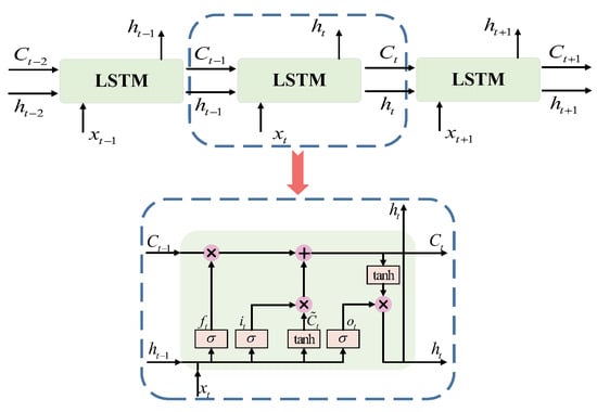
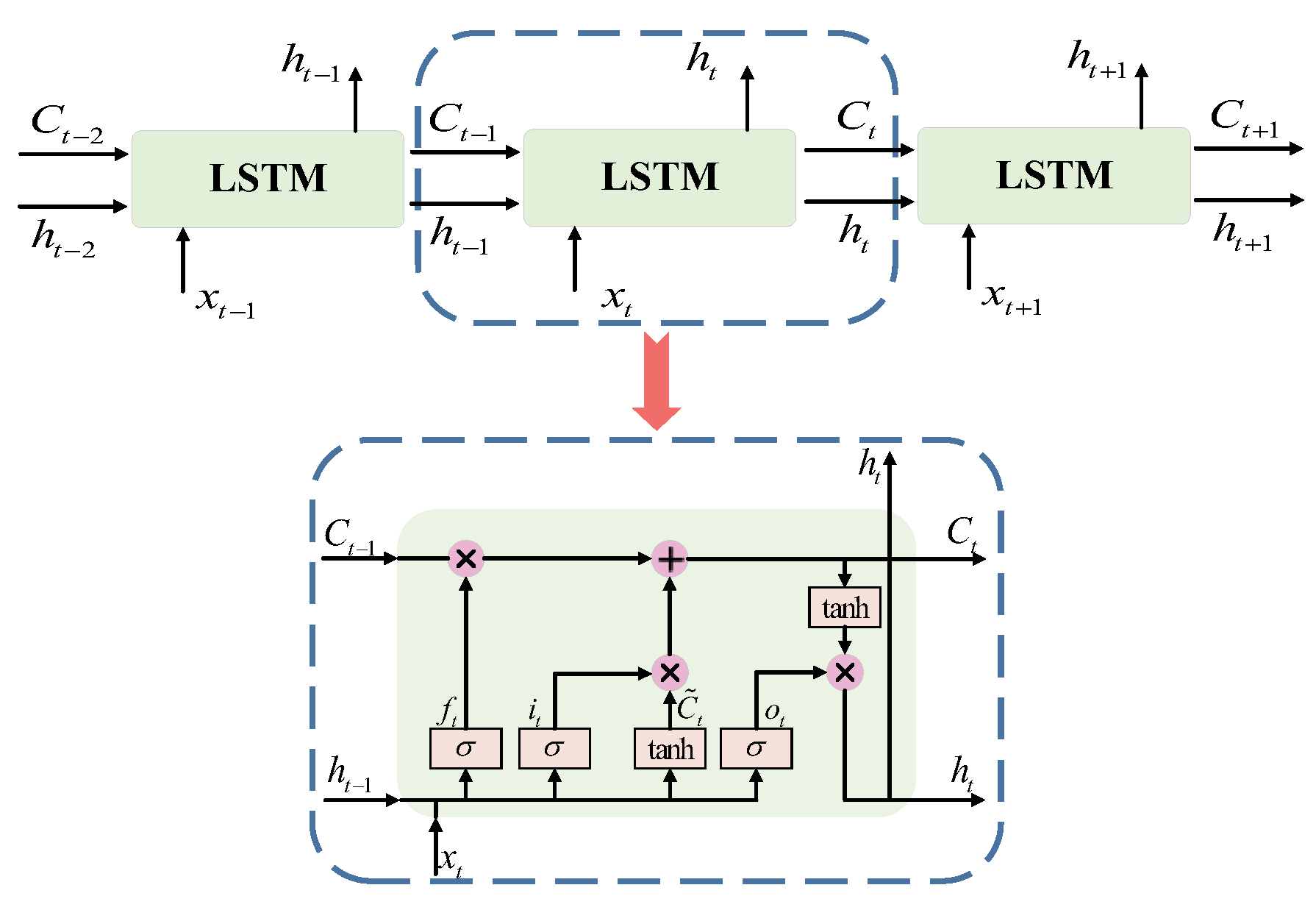
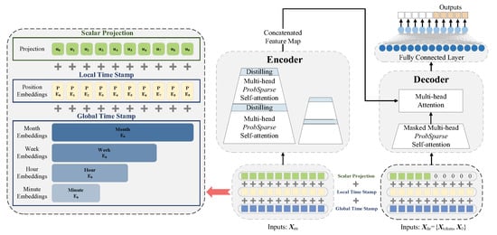
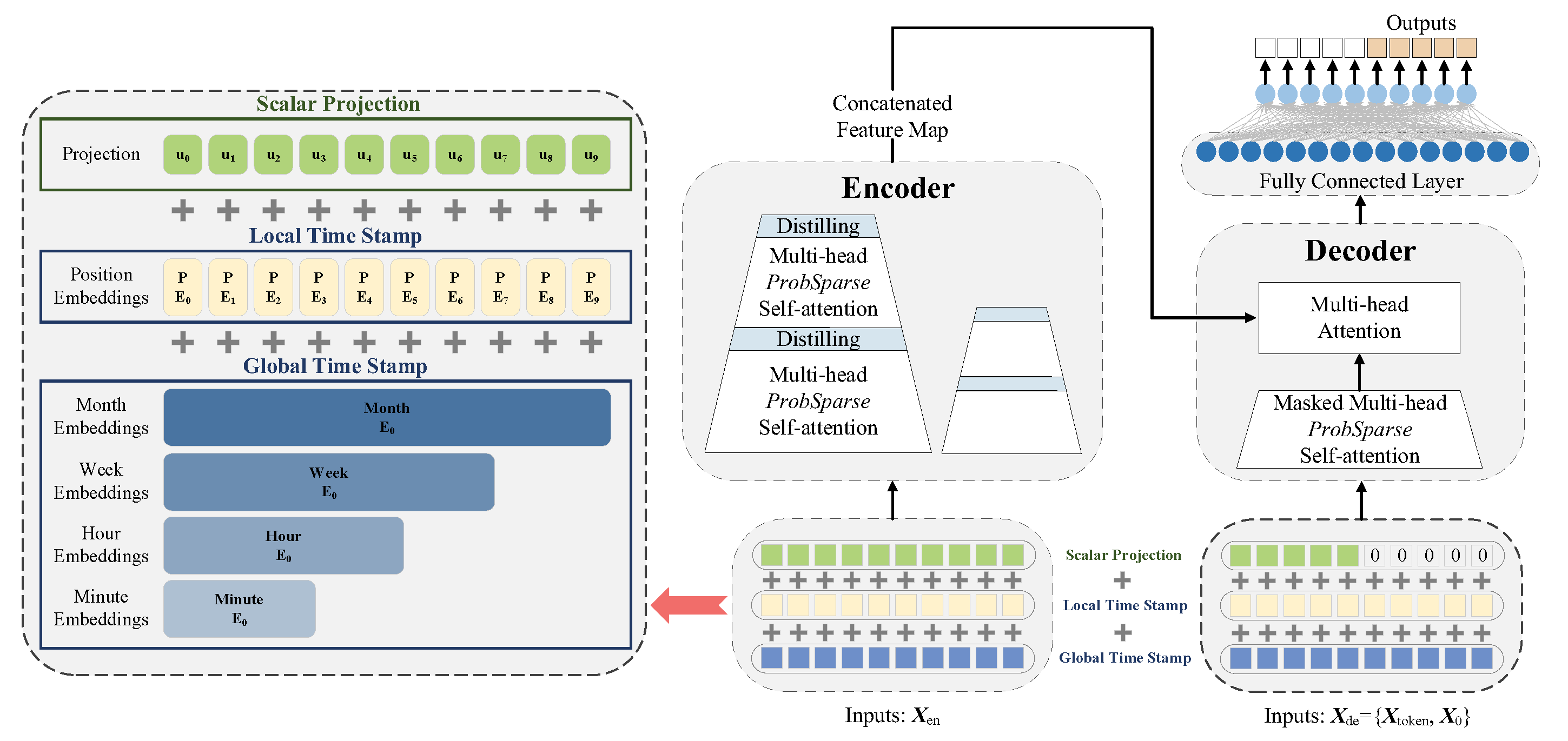
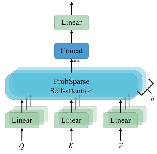
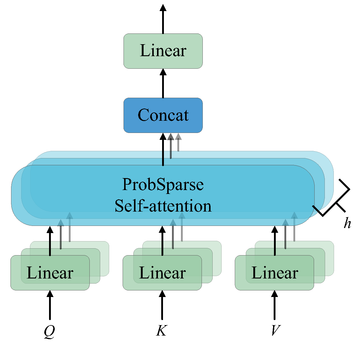
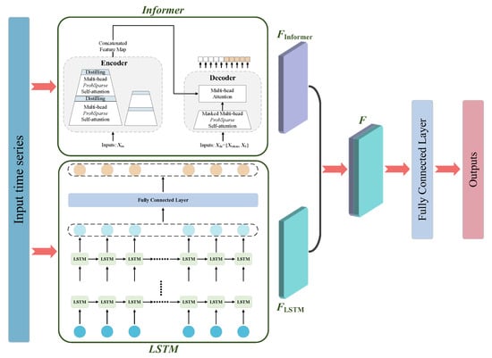
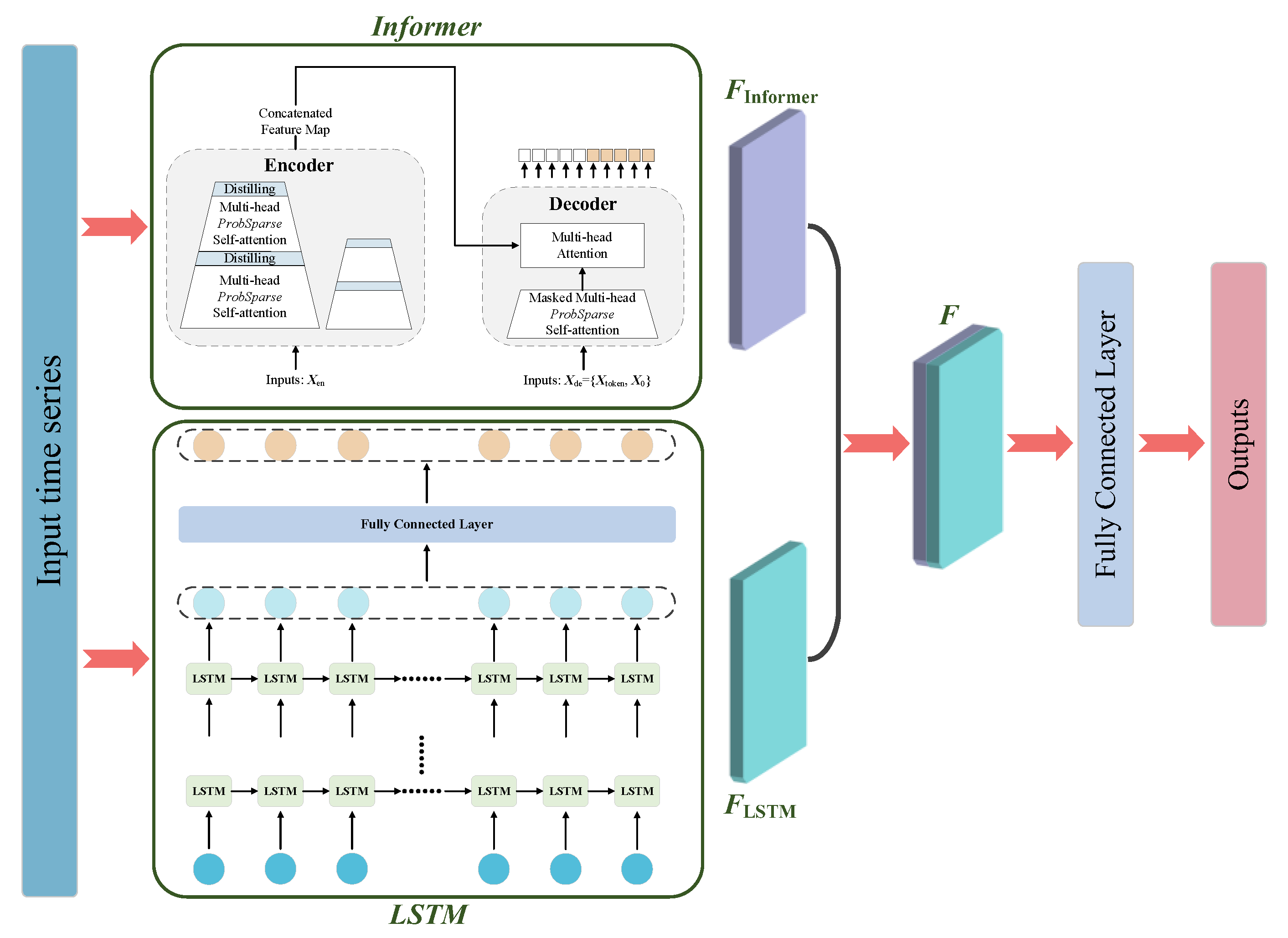
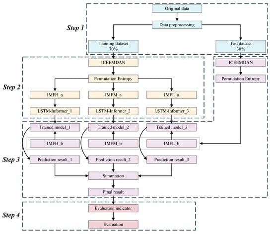
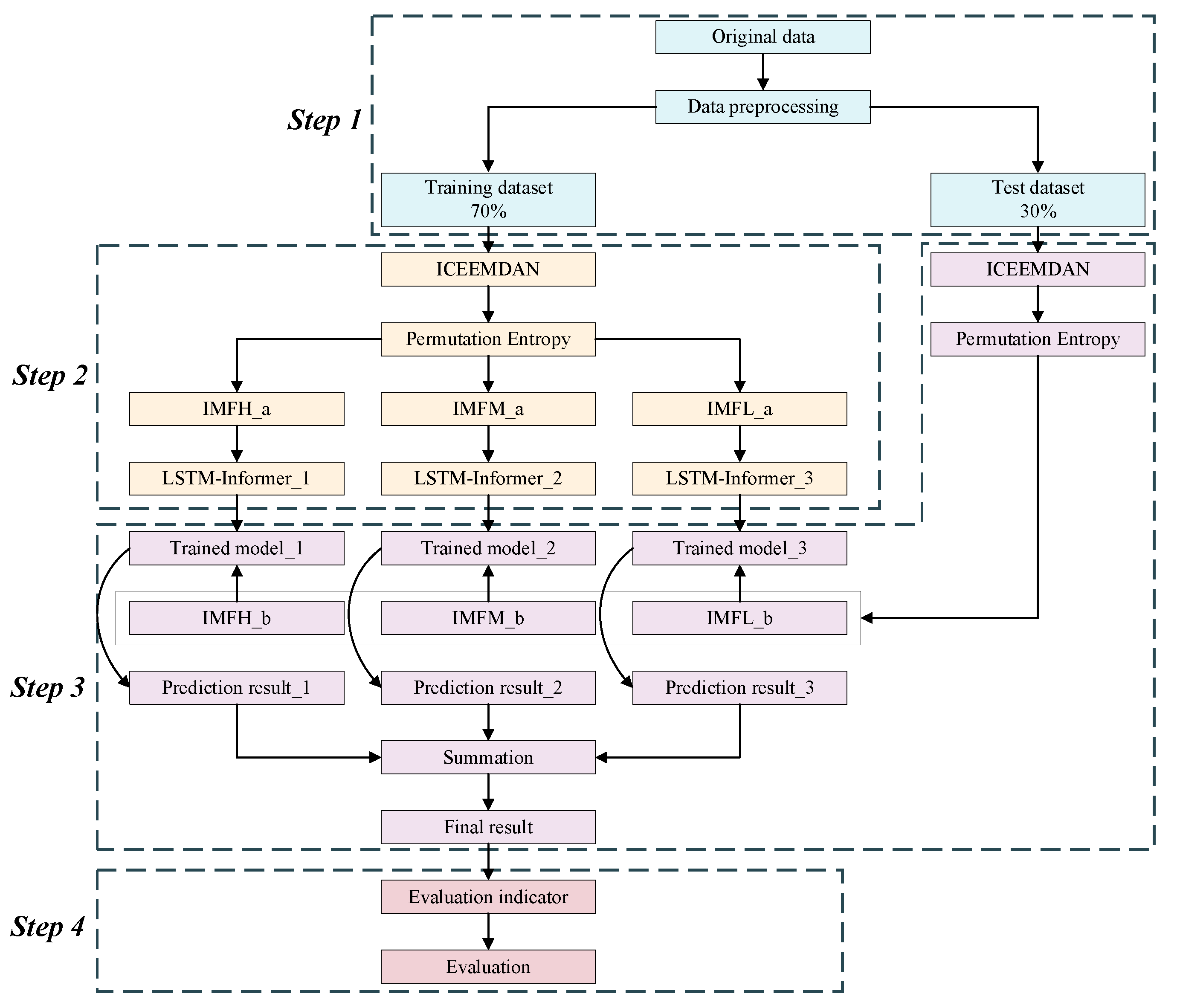
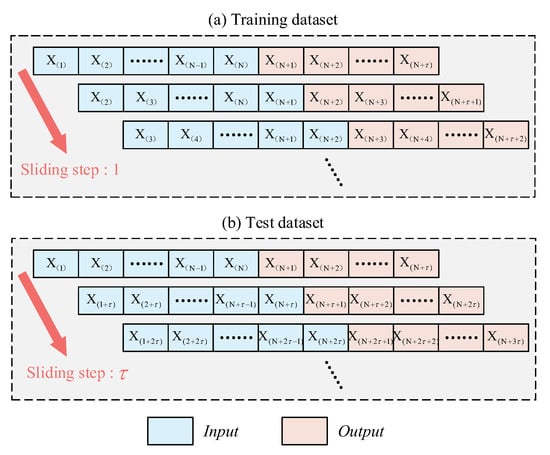
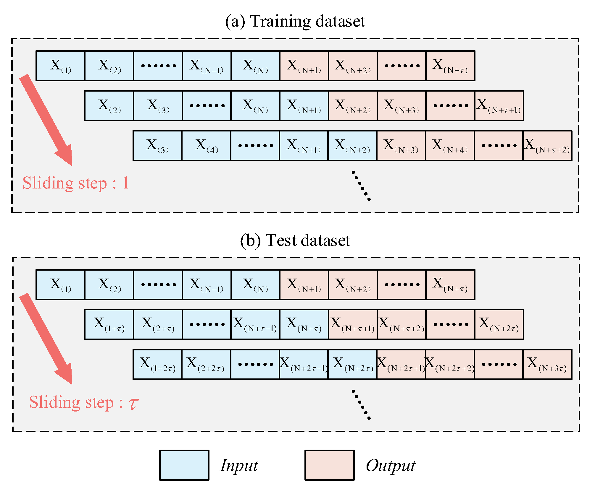
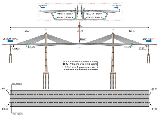
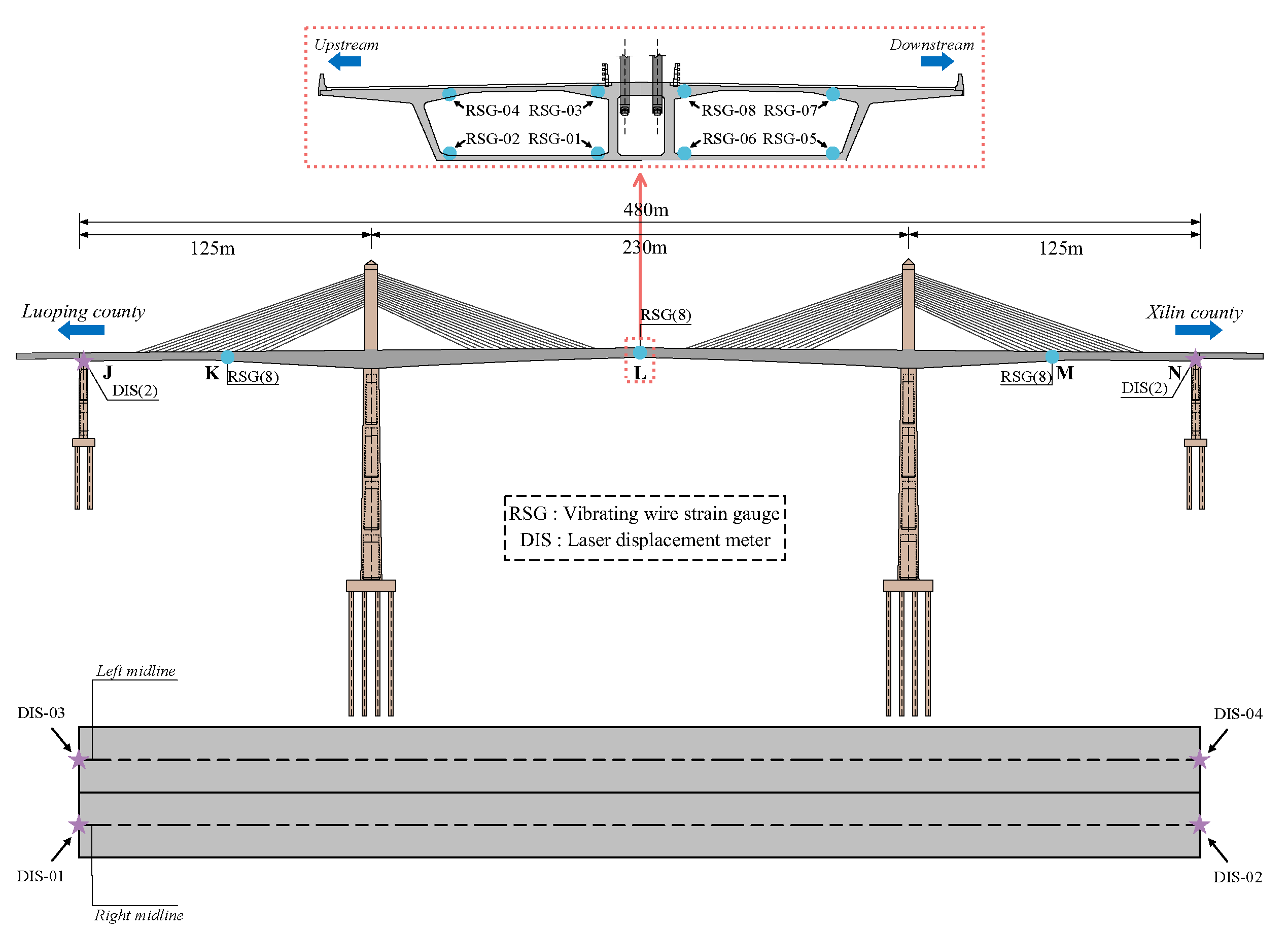
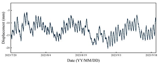
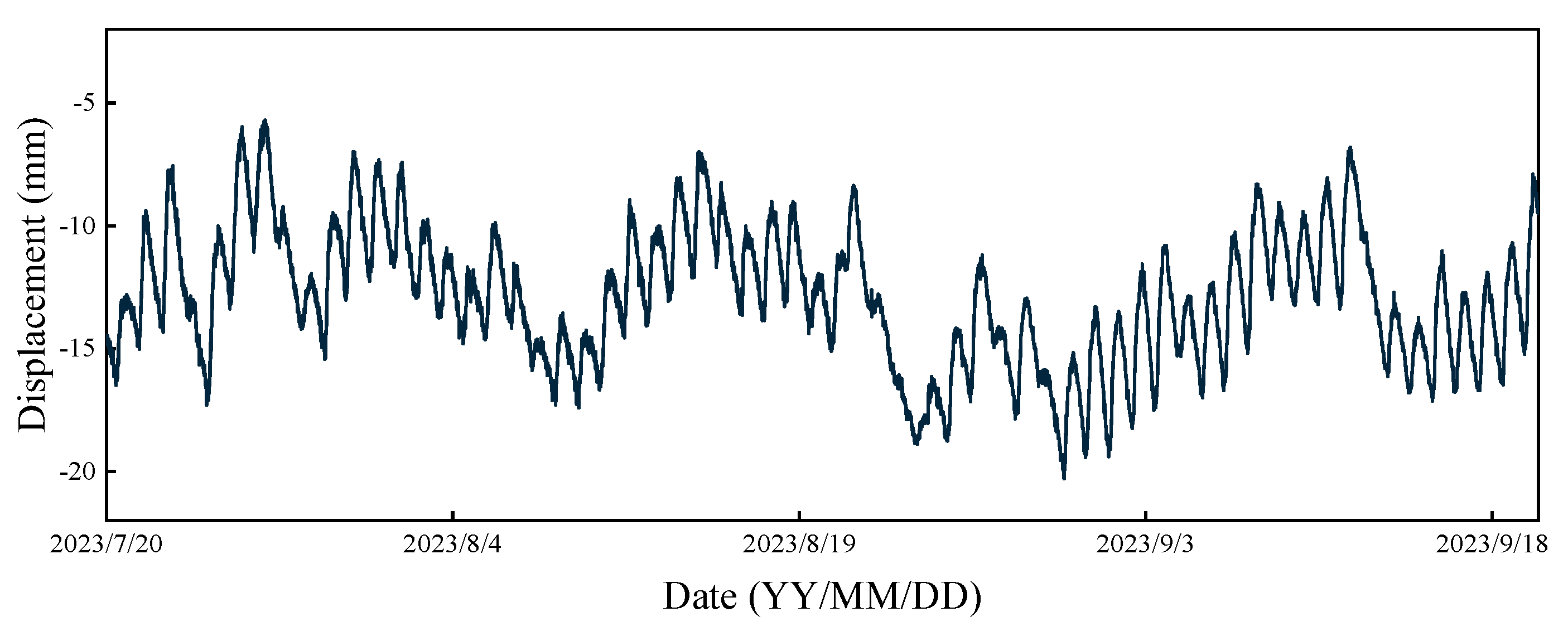
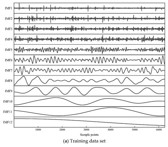
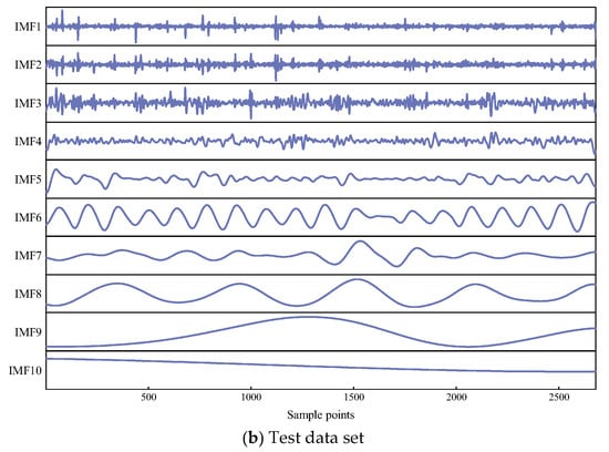
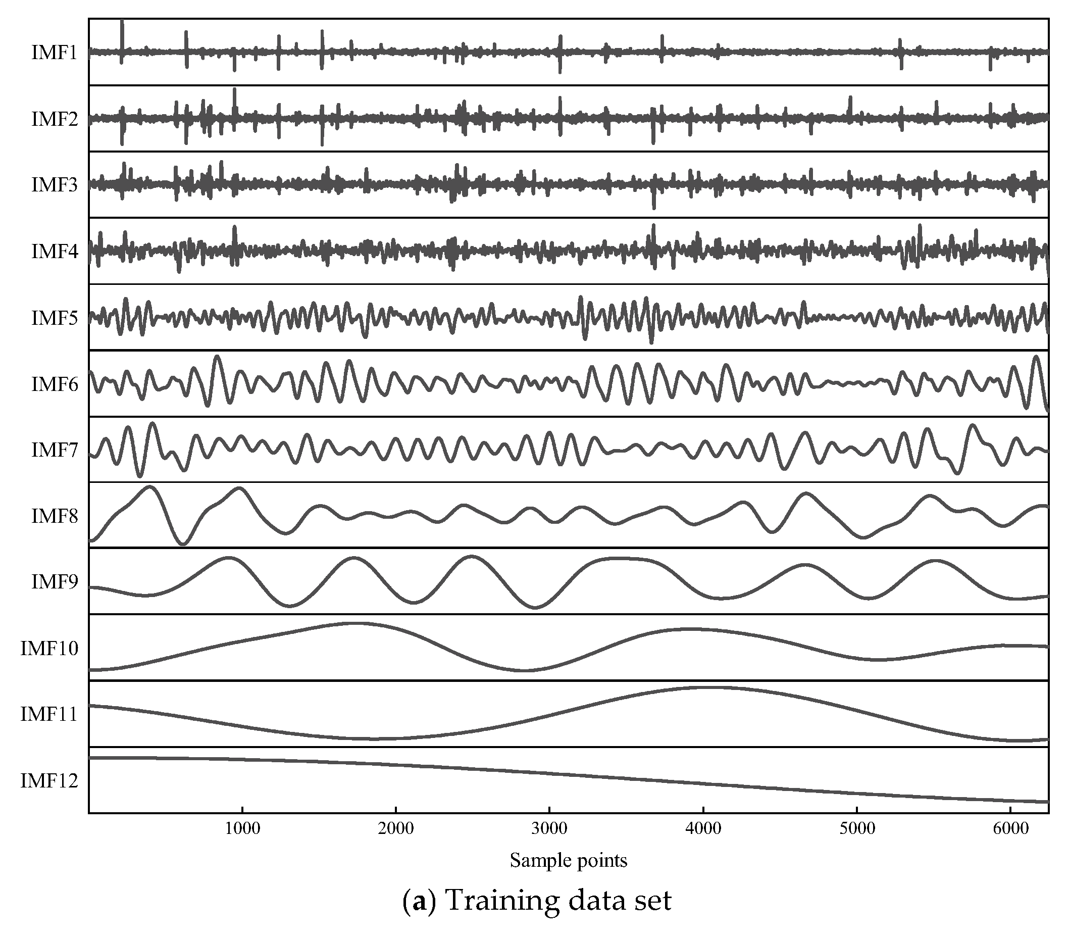
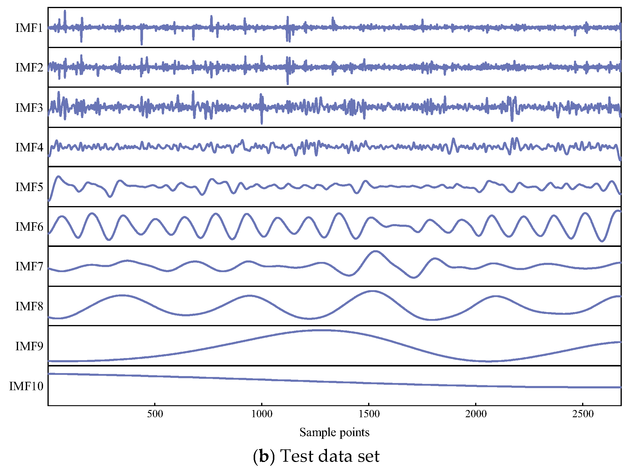
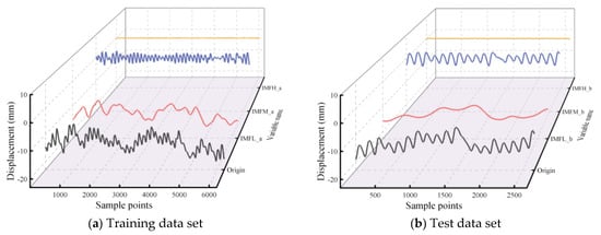
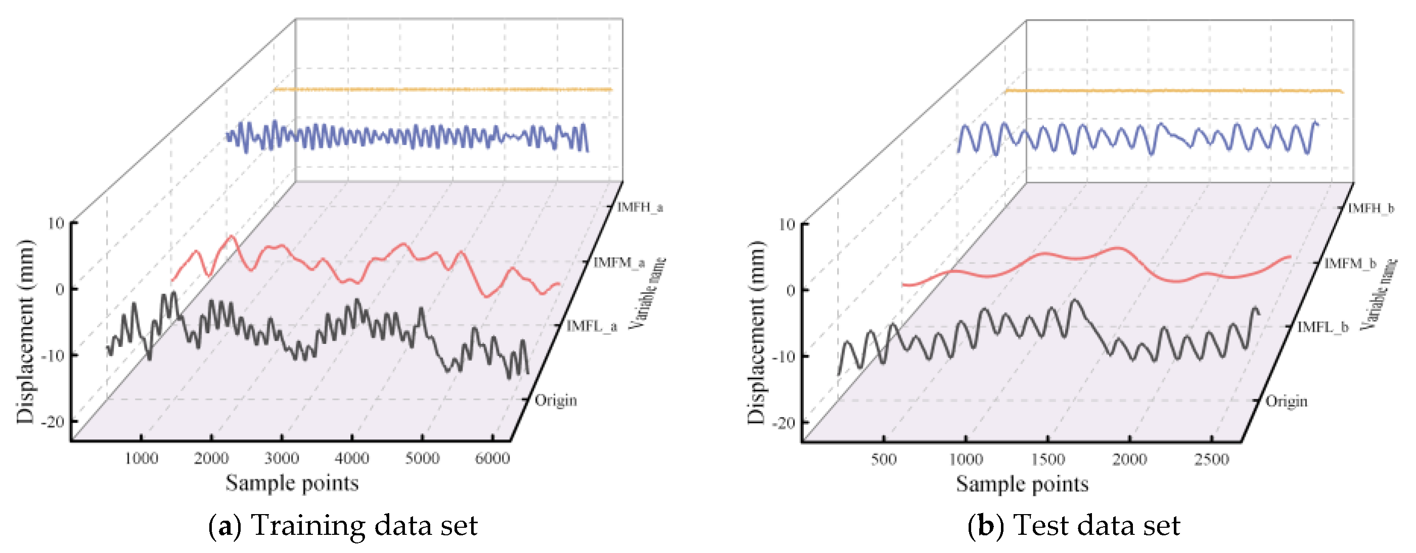
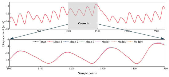
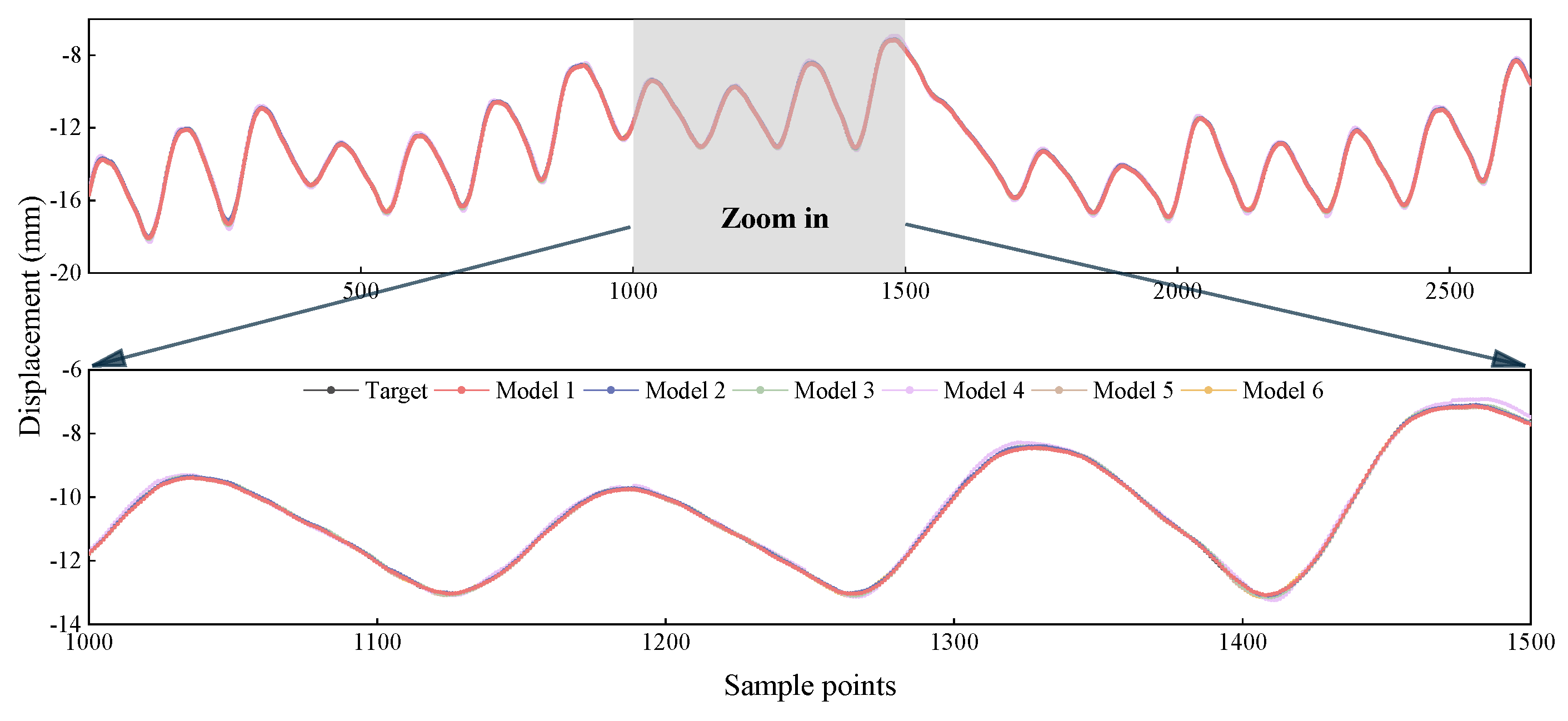
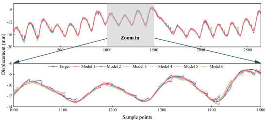
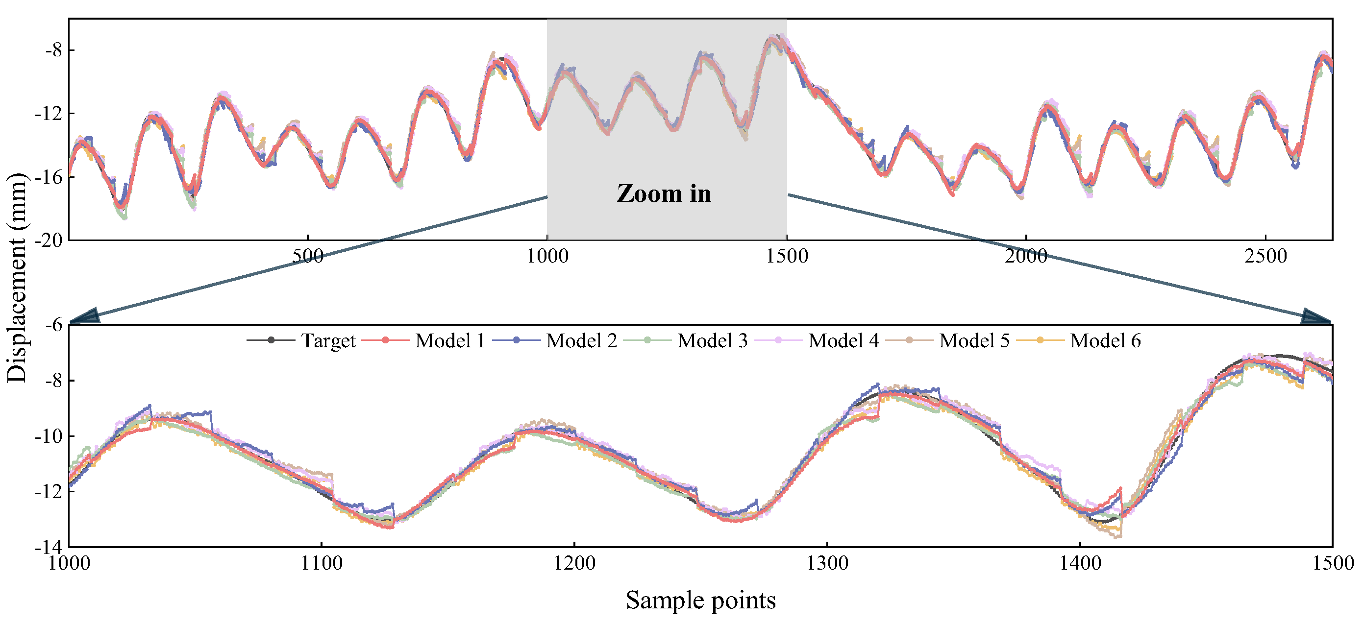
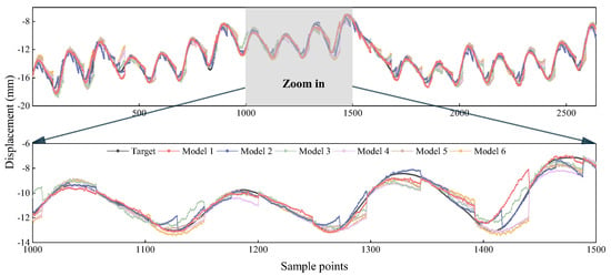
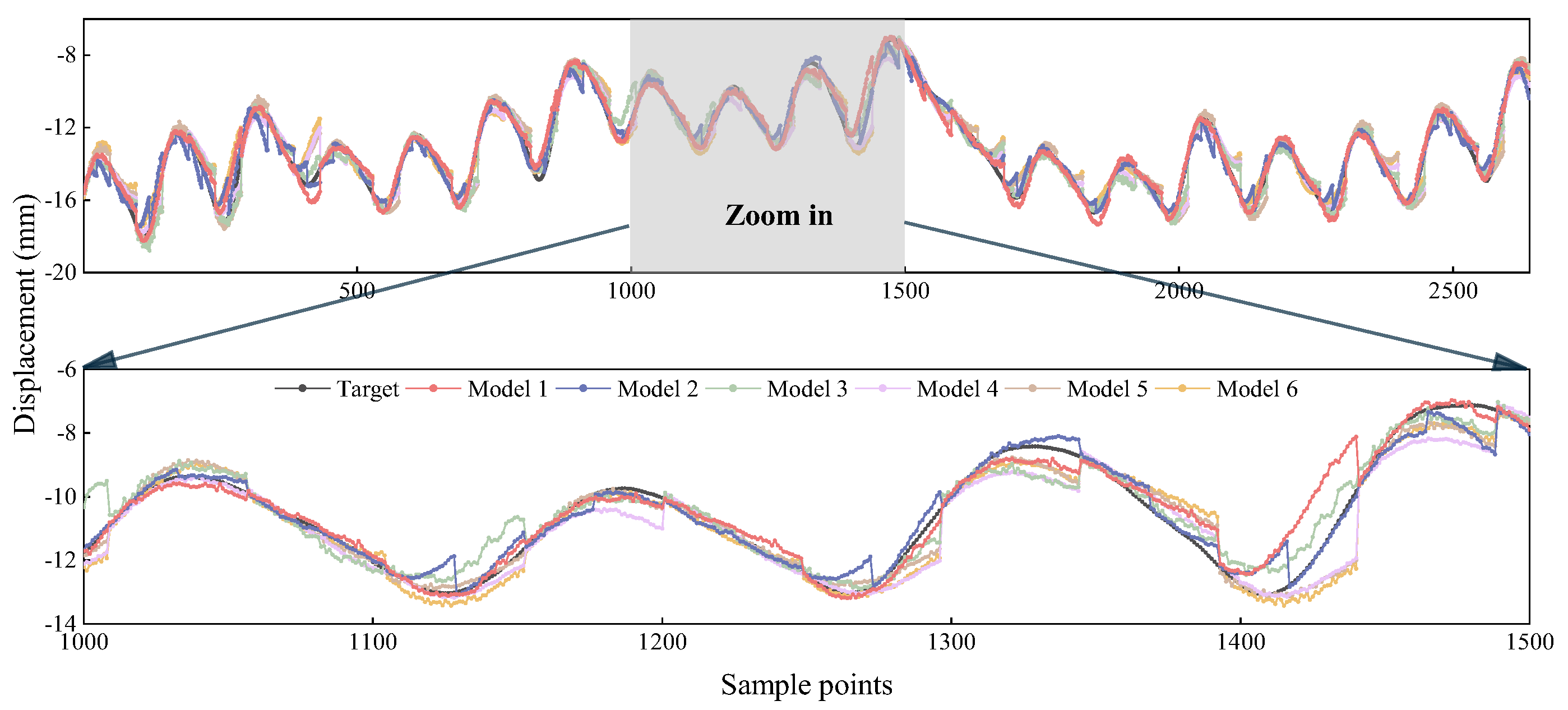
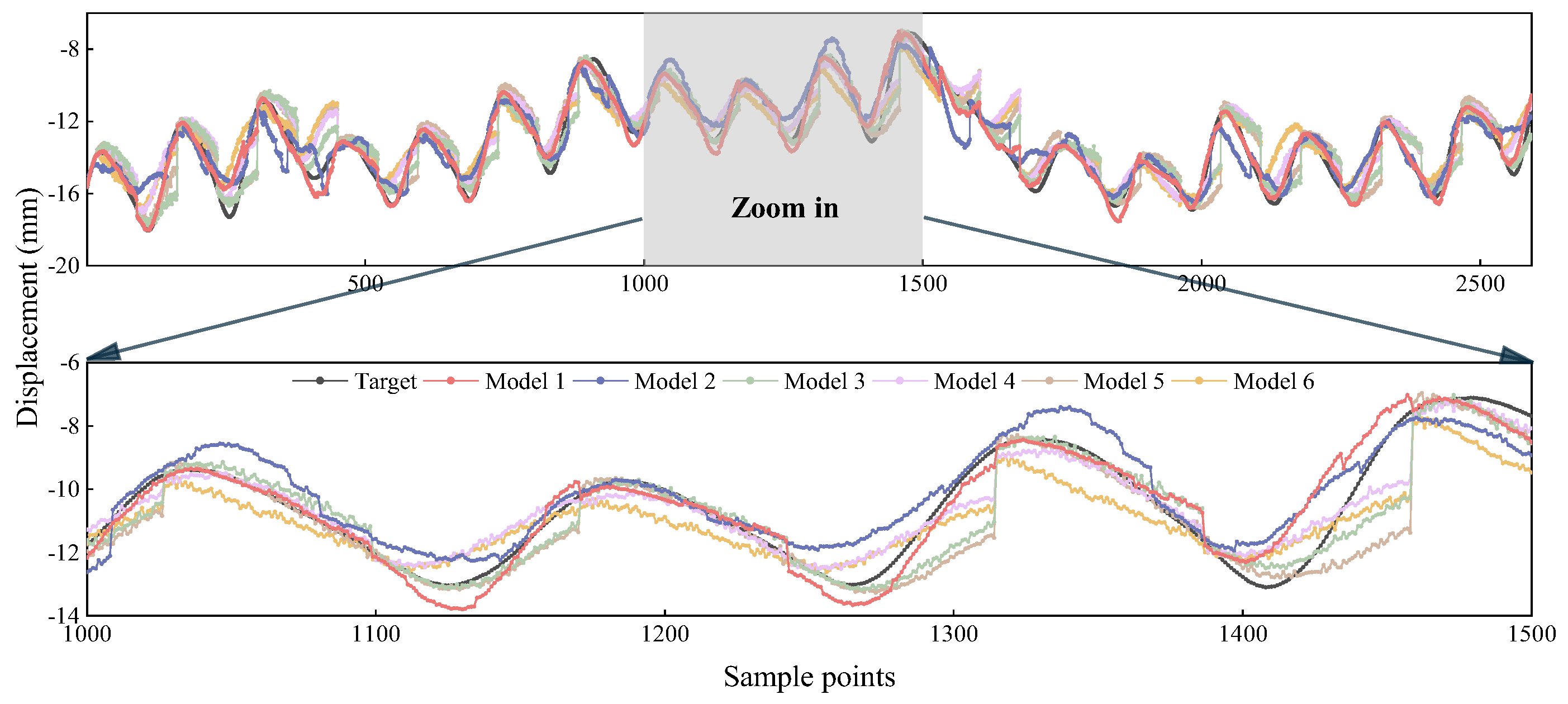
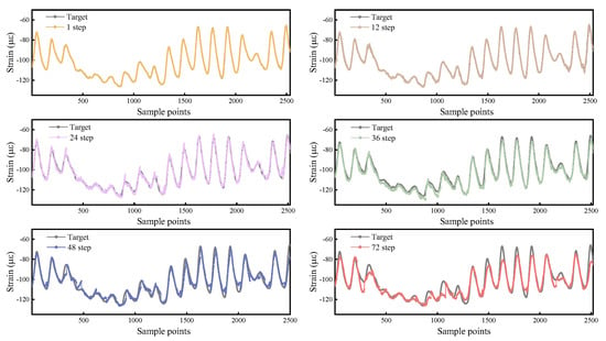
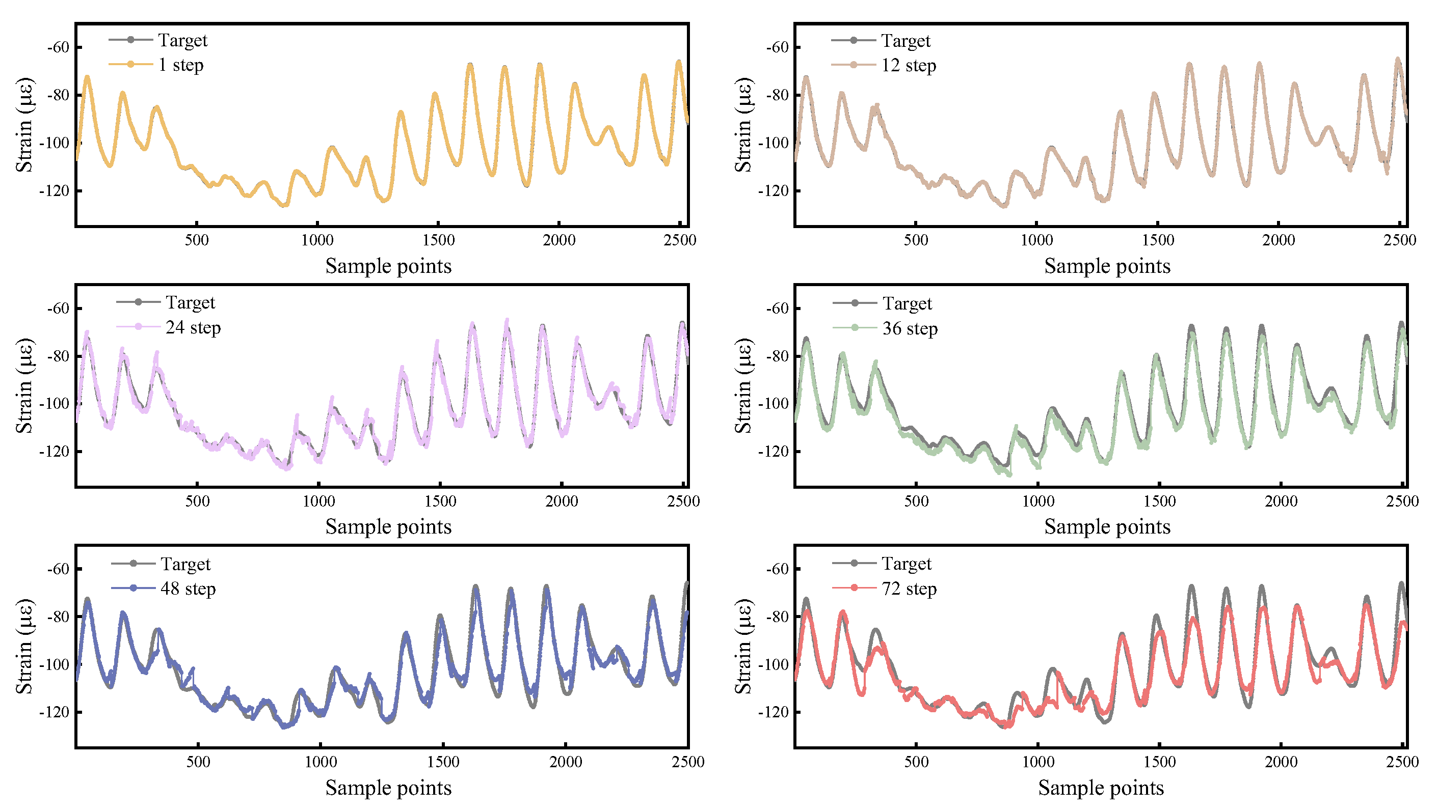
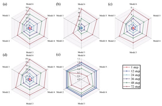
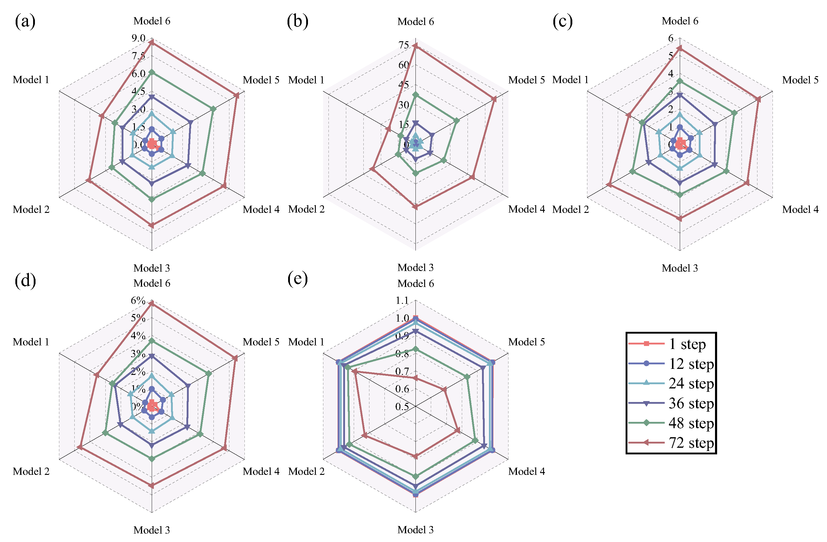

Disclaimer/Publisher’s Note: The statements, opinions and data contained in all publications are solely those of the individual author(s) and contributor(s) and not of MDPI and/or the editor(s). MDPI and/or the editor(s) disclaim responsibility for any injury to people or property resulting from any ideas, methods, instructions or products referred to in the content. |
© 2026 by the authors. Licensee MDPI, Basel, Switzerland. This article is an open access article distributed under the terms and conditions of the Creative Commons Attribution (CC BY) license.