Foreground-Guided and Geometry-Confusion-Aware Transformer for Damaged Component Detection in Urban Buildings

Abstract

To address the need for detecting damaged regions that develop during the long-term service of urban landscape buildings, existing vision-based detection methods are easily affected by background interference such as shadows, decorative textures, and component joints in complex scenes. They also face substantial inter-class visual similarity and pronounced intra-class variations in target scale, aspect ratio, and appearance. To address these challenges, this paper proposes a Foreground-Guided and Geometry-Confusion-Aware Network (FGCNet). First, a foreground-guided wavelet modulation module constructs foreground–background contrast statistics for individual wavelet subbands and performs spatially constrained band modulation to enhance damage-related features with low visual contrast. Second, a Geometry-Confusion Aware Networkare class-prototype contrast branch mines hard negative classes using online confusion relationships from the base classifier, thereby improving discrimination between visually similar classes. Finally, a geometry-aware intra-class multi-prototype mechanism jointly exploits query appearance and predicted bounding-box geometry to adaptively model latent patterns within the same class. Experiments are conducted on an urban landscape building dataset containing 10 categories of damaged regions. The results show that FGCNet improves mAP_50:95 and mAP₅₀ over the baseline by 2.6 and 3.7 percentage points, respectively. The proposed method can provide technical support for visual inspection and damage-information recording in complex urban landscape building scenes.

1. Introduction

Urban landscape buildings play an important role in shaping the urban image, representing regional culture, and maintaining the integrity of landscape spaces. Because they remain exposed to open environments over long service periods, they are susceptible to rainfall erosion, temperature variation, biological attachment, visitor contact, and inadequate maintenance. Unlike sudden post-disaster damage [1,2], deterioration in these buildings may gradually accumulate and propagate during long-term service. If cracks, finish spalling, component corrosion, or connection damage are not detected in a timely manner, they may not only degrade the visual quality of the built landscape but also create public-safety hazards such as falling finishes or components. For pavilions, towers, memorial archways, and other structures with historical character and cultural significance, material deterioration may additionally cause irreversible losses of historical information and artistic value [3,4]. Therefore, this capability is crucial for accurately detecting damaged components in urban landscape buildings.

Research on the digital inspection of historic buildings and cultural heritage provides important references for damage analysis of urban landscape buildings. Galantucci et al. used digital photogrammetry to construct two- and three-dimensional models of historic buildings and extracted information on cracks, material loss, erosion, and other deterioration through three-dimensional surface analysis, demonstrating that non-contact measurement can support quantitative recording and multi-temporal comparison of building surface conditions [5]. Pathak et al. formulated cracks and spalling in cultural heritage buildings as an object-detection task, analyzed two-dimensional images using Faster R-CNN, and mapped the detection results to three-dimensional point-cloud models, enabling damage localization and visualization under complex architectural texture backgrounds [6]. Samhouri et al. employed convolutional neural networks to identify erosion, material loss, stone discoloration, and human-induced damage on historic building facades and further attempted to measure the extent of deterioration [7]. For wooden architectural heritage, Lee and Yu established an on-site image dataset, compared multiple convolutional neural networks, and used class activation mapping to interpret the regions attended to by the models [8]; for stone buildings, Idjaton et al. combined YOLOv5 with a Transformer architecture using highly overlapping images acquired during three-dimensional surveying to automatically identify limestone spalling [9].

With the rapid development of artificial intelligence and computer vision, together with the continuing evolution of architectural-conservation concepts, building damage inspection has gradually shifted from conventional contact-based inspection toward efficient and non-destructive non-contact approaches [10]. Non-contact techniques such as infrared imaging and digital image processing [11,12,13,14,15] have been widely applied to the conservation of urban landscape buildings and provide important technical support for automated damage detection from visual information. Uysal et al. constructed digital-twin models of cultural heritage buildings through UAV photogrammetry and automatically detected and measured cracks in highly textured three-dimensional models, providing a technical route for non-contact inspection of inaccessible areas [16]. Xu and Chen focused on ancient towers and combined UAV imagery, photogrammetry, an improved object-detection algorithm, and a digital-twin platform to identify cracks and corrosion damage from multiple viewpoints [17]. Huang et al. further integrated image classification, semantic segmentation, and scale calibration to identify surface cracks in cultural heritage while calculating their actual lengths [18]. From the broader perspective of infrastructure operation and maintenance, digital twins can associate building geometry, damage-detection results, historical inspection records, and dynamic monitoring information, thereby providing a unified data carrier for damage-evolution analysis and maintenance management [19]. Existing studies have therefore established a technical evolution path from two-dimensional image classification, object detection, and pixel-level segmentation to three-dimensional reconstruction, spatial mapping, and digital-twin management.

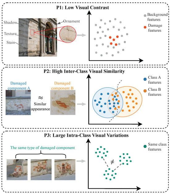
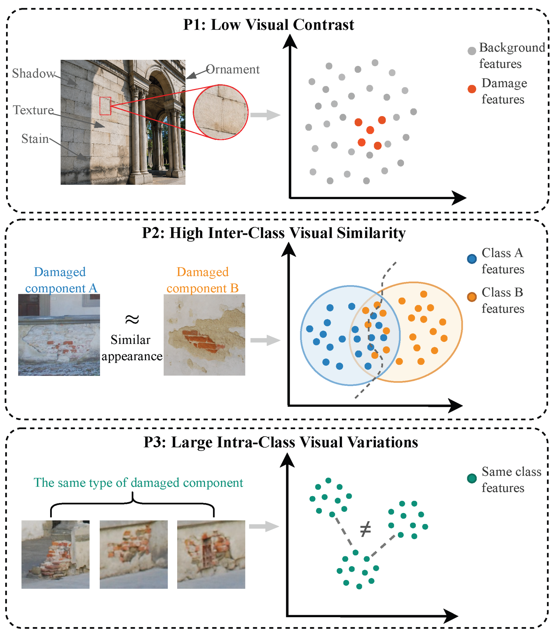
However, directly applying the above methods to damaged components in urban landscape buildings remains challenging due to the following reasons. These challenges can be summarized into three aspects, as shown in Figure 1. (1) Low visual contrast. There is low visual contrast between damaged components and the surrounding normal components. Urban landscape buildings commonly contain multiple materials, including wood, stone, brick, concrete, and finishing materials. Their surfaces may simultaneously exhibit decorative textures, component joints, natural aging traces, and environmental attachments while also being affected by illumination changes, shadows, vegetation occlusion, and visitor activity [8,9,16,17,18,19,20]. Fine cracks, early-stage corrosion, and slight spalling are often manifested only as subtle local variations in color, texture, or edges, with limited grayscale and texture differences from surrounding material surfaces. (2) High inter-class visual similarity. Damaged components of different categories exhibit similar visual damage features. For example, slender cracks and component joints both exhibit linear edge characteristics, while material spalling and surface weathering may both appear as irregular regions with abrupt texture changes. When different damage classes share similar local shape, texture, and color cues, their deep features can overlap in representation space, preventing the model from forming clear and stable class decision boundaries and consequently causing class confusion. Although existing methods can classify or localize cracks, spalling, corrosion, and other deterioration, their ability to represent fine-grained differences between visually similar categories remains limited. (3) Large intra-class visual variations. The same type of damaged component can exhibit diverse visual damage features. For cracks, width, length, orientation, continuity, and branching morphology vary with material type, damage stage, and imaging scale. Spalling may likewise exhibit markedly different colors, boundaries, and textures depending on the substrate material, development stage, and illumination conditions. Consequently, samples belonging to the same class may be widely dispersed in feature space, making stable class representations difficult to learn. Accordingly, this study proposes a method for detecting and assessing damaged regions in urban landscape buildings.

Figure 1. Three major challenges in damage detection for urban landscape buildings.

• We construct an image dataset of architectural damage in urban landscapes and propose FGCNet, an end-to-end framework for automatically identifying and localizing damaged components in complex scenes.
• We propose a foreground-guided wavelet modulation method that enhances edge and texture responses in damaged regions through spatially constrained frequency-band modulation, thereby reducing interference from complex architectural backgrounds during feature extraction.
• We develop a collaborative discriminative mechanism composed of Confusion-Aware Class-Prototype Contrast (CAPC) and Geometry-Aware Intra-class Multi-Prototype (GAMP) to address visual similarity between different building components and large intra-class variations in scale, aspect ratio, and appearance.

The paper is organized as follows. Section 2 presents the details of the proposed algorithm. Section 3 assesses the performance of the solution and presents the numerical results. Finally, the conclusions remarks are given in Section 4.

2. Proposed Method

2.1. Method Overview

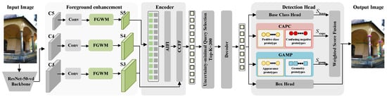
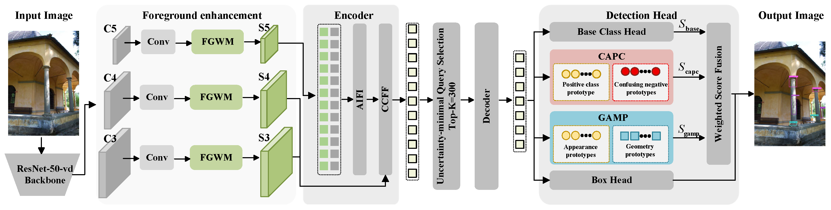
We propose a Foreground-Guided and Geometry-Confusion-Aware Network (FGCNet) for damage detection in urban landscape buildings, as illustrated in Figure 2. The network adopts RT-DETR-R50-vd [21] as the base detector and is specifically designed around three key challenges in urban landscape building damage detection. First, the visual contrast between damaged regions and shadows, joints, or decorative textures is often low, which can lead to insufficient foreground responses. To address this issue, Foreground-Guided Wavelet Modulation (FGWM) is introduced before the multi-scale projected features enter the Hybrid Encoder. FGWM uses predicted foreground weights to construct foreground–background contrast statistics for each wavelet subband and enhances damage-related information through spatially constrained band modulation. Second, different damage classes may share similar local textures and edges, resulting in ambiguous inter-class decision boundaries. Therefore, Confusion-Aware Class-Prototype Contrast (CAPC) is introduced at the classification stage of the final Decoder queries. CAPC mines hard negative classes using online confusion relationships and enlarges the margins between easily confused categories in the class-prototype space. Finally, damage instances of the same class can vary substantially in scale, aspect ratio, and appearance, such that a single class center cannot adequately cover the intra-class distribution. To address this issue, Geometry-Aware Intra-class Multi-Prototype (GAMP) uses paired appearance–geometry prototypes to represent latent modes within a class and adaptively aggregates the matching modes according to the current query. FGWM operates on the encoder input features, whereas CAPC and GAMP provide complementary logits to the classification head. The three modules are not simply cascaded, and the original Box Head remains unchanged.

Figure 2. Overall architecture of FGCNet. The input image is processed by ResNet-50-vd to extract three-scale features, which are projected to 256 channels and then enhanced by the shared FGWM in a foreground-guided manner. The RT-DETR Hybrid Encoder and a six-layer Deformable Transformer Decoder generate 300 queries. The final queries are fed in parallel to the base classification head, CAPC, and GAMP. The three sets of class logits are fused using weighted score fusion and combined with the output of the independent Box Head to produce NMS-free detection results.

Given an RGB image of a building surface $\mathbf{I}\in {\mathbb{R}}^{3\times H_0\times W_0}$, its annotation set is denoted as

$$\mathcal{Y}={\left\{(y_j,{\mathbf{b}}_j)\right\}}_{j=1}^G,{\mathbf{b}}_j=[x_j,y_j,w_j,h_j],$$

(1)

where $y_j\in \{1,\dots ,N\}$ denotes the class of the damaged component, ${\mathbf{b}}_j$ is the normalized bounding box, and N excludes the background class. FGCNet outputs a set prediction corresponding to $K=300$ queries,

$$\widehat{\mathcal{Y}}={\left\{({\widehat{\mathbf{s}}}_i,{\widehat{\mathbf{b}}}_i)\right\}}_{i=1}^K,{\widehat{\mathbf{s}}}_i\in {\mathbb{R}}^N,{\widehat{\mathbf{b}}}_i\in {[0,1]}^4.$$

(2)

The model adopts the one-to-one Hungarian matching and end-to-end set prediction of RT-DETR and does not perform NMS during inference. FGCNet outputs the damage class and its location but does not directly predict damage severity or maintenance decisions; the latter two are independent assessment tasks conducted after detection.

2.2. Overall Architecture of FGCNet

For an input image of size $640\times 640$, ResNet-50-vd outputs $C_3$, $C_4$, and $C_5$ features with strides of 8, 16, and 32, respectively. Three $1\times 1$ convolutions unify the channel dimension to $C=256$, after which the features are separately fed into FGWM modules with a shared structure:

$$\begin{array}{cc}\hfill {\mathbf{F}}^{\ell }& ={\mathrm{Conv}}_{1\times 1}\left({\mathbf{C}}^{\ell }\right),\hfill \\ \hfill {\mathbf{F}}_{\mathrm{fg}}^{\ell }& =\mathrm{FGWM}\left({\mathbf{F}}^{\ell }\right),\ell \in \{3,4,5\}.\hfill \end{array}$$

(3)

At the illustrated resolution, the three feature maps have sizes of $256\times 80\times 80$, $256\times 40\times 40$, and $256\times 20\times 20$, respectively. The enhanced features are fed into the original RT-DETR Hybrid Encoder, in which AIFI operates on the highest-level feature to model long-range dependencies at the same scale, while CCFF performs cross-scale fusion through top-down and bottom-up pathways. The encoder outputs are flattened and concatenated as

$$\begin{array}{cc}\hfill \mathbf{E}& =\mathrm{Flatten}\left({\mathbf{E}}_3\right)\parallel \mathrm{Flatten}\left({\mathbf{E}}_4\right)\hfill \\ \hfill & \parallel \mathrm{Flatten}\left({\mathbf{E}}_5\right)\in {\mathbb{R}}^{8400\times 256}.\hfill \end{array}$$

(4)

where $8400=80\times 80+40\times 40+20\times 20$. Following the uncertainty-minimal Top-K query selection of RT-DETR, $K=300$ initial queries and reference boxes are selected from the encoder candidates. A six-layer Deformable Transformer Decoder then produces the final queries $\mathbf{Q}$ and Box Head predictions $\mathbf{B}$:

$$\mathbf{Q}\in {\mathbb{R}}^{300\times 256},\mathbf{B}\in {\mathbb{R}}^{300\times 4}.$$

(5)

The backbone, Hybrid Encoder, query selection, Decoder, and Box Head are inherited from RT-DETR-R50-vd. The modifications introduced in this study are concentrated in FGWM and the two complementary classification branches.

The final queries are simultaneously fed into the base classification head, the CAPC branch, and the GAMP branch to obtain ${\mathbf{S}}_{\mathrm{base}}$, ${\mathbf{S}}_{\mathrm{capc}}$, and ${\mathbf{S}}_{\mathrm{gamp}}\in {\mathbb{R}}^{300\times N}$. The three sets of logits are combined through residual weighted fusion:

$${\mathbf{S}}_{\mathrm{final}}={\mathbf{S}}_{\mathrm{base}}+{\eta }_1{\mathbf{S}}_{\mathrm{capc}}+{\eta }_2{\mathbf{S}}_{\mathrm{gamp}}.$$

(6)

where ${\eta }_1=0.3$ and ${\eta }_2=0.2$ are fixed logit-fusion coefficients and are not learned during training. Equation (6) fuses logits rather than averaging probabilities. The Box Head output $\mathbf{B}$ does not participate in score fusion, and the final result is composed of $({\mathbf{S}}_{\mathrm{final}},\mathbf{B})$.

2.3. FGWM: Foreground-Guided Wavelet Modulation

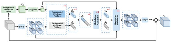
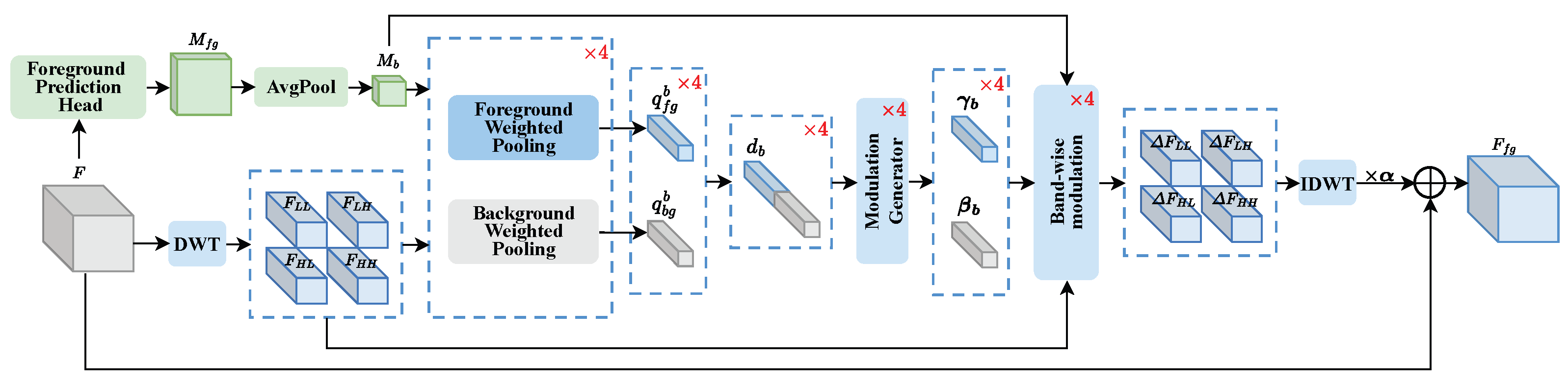
Shadows, joints, decorative textures, and non-uniform illumination on building surfaces can simultaneously produce low-frequency appearance variations and high-frequency edge responses. Indiscriminately enhancing high-frequency information can cause weak damage cues to be overwhelmed by background textures. FGWM is placed after the three-scale projection and before the Hybrid Encoder. It uses foreground weights obtained through weak box supervision to separately summarize foreground and background responses within each wavelet subband and performs spatially constrained modulation only at locations with high foreground probability, as illustrated in Figure 3.

Figure 3. Structure of FGWM. The input feature $\mathbf{F}$ is processed by a lightweight Foreground Prediction Head to obtain the foreground weight ${\mathbf{M}}_{\mathrm{fg}}$ and is also decomposed into four wavelet subbands using DWT. Foreground/background weighted pooling is performed for each wavelet subband to generate band-specific modulation parameters. The enhanced feature ${\mathbf{F}}_{\mathrm{fg}}$ is then obtained through spatially constrained increments, IDWT, and a residual connection.

For an input feature $\mathbf{F}\in {\mathbb{R}}^{C\times H\times W}$ at any scale, the Foreground Prediction Head forms a lightweight branch using a $3\times 3$ convolution, normalization, SiLU, and a $1\times 1$ convolution, and outputs a continuous foreground weight

$$\begin{array}{cc}\hfill {\mathbf{H}}_{\mathrm{fg}}& =\mathrm{SiLU}\left(\mathrm{Norm}\left({\mathrm{Conv}}_{3\times 3}\left(\mathbf{F}\right)\right)\right),\hfill \\ \hfill {\mathbf{M}}_{\mathrm{fg}}& =\sigma \left({\mathrm{Conv}}_{1\times 1}\left({\mathbf{H}}_{\mathrm{fg}}\right)\right)\in {[0,1]}^{1\times H\times W}.\hfill \end{array}$$

(7)

During training, XML bounding boxes are rasterized into a box-derived target ${\mathbf{T}}_{\mathrm{fg}}$, with locations covered by a bounding box assigned a value of 1 and all other locations assigned 0. This target only indicates that regions inside the box have a higher probability of being damage foreground and is not a pixel-accurate segmentation mask. The foreground-branch loss is

$${\mathcal{L}}_{\mathrm{fg}}^{\ell }=\mathrm{FocalBCE}({\mathbf{M}}_{\mathrm{fg}}^{\ell },{\mathbf{T}}_{\mathrm{fg}}^{\ell }),{\mathcal{L}}_{\mathrm{fg}}={\displaystyle \sum _{\ell =3}^5}{\mathcal{L}}_{\mathrm{fg}}^{\ell }.$$

(8)

During inference, ${\mathbf{M}}_{\mathrm{fg}}$ is predicted entirely from the input features and does not access XML annotations or Ground Truth.

A one-level two-dimensional discrete wavelet transform decomposes $\mathbf{F}$ into a low-frequency structural component and three directional high-frequency wavelet subbands:

$$\begin{array}{cc}\hfill {\left\{{\mathbf{F}}_b\right\}}_{b\in \mathcal{B}}& =\mathrm{DWT}\left(\mathbf{F}\right),\hfill \\ \hfill \mathcal{B}& =\{LL,LH,HL,HH\},\hfill \\ \hfill {\mathbf{F}}_b& \in {\mathbb{R}}^{C\times H/2\times W/2}.\hfill \end{array}$$

(9)

where $LL$ preserves overall structural and appearance information, whereas $LH$, $HL$, and $HH$ describe edges and textures in different directions. Average pooling with both kernel size and stride equal to 2 is applied once to align the foreground weight with the wavelet subband resolution:

$${\mathbf{M}}_b={\mathrm{AvgPool}}_{2\times 2}\left({\mathbf{M}}_{\mathrm{fg}}\right)\in {[0,1]}^{1\times H/2\times W/2}.$$

(10)

For any wavelet subband $b\in \{LL,LH,HL,HH\}$, normalized weighted pooling is performed using ${\mathbf{M}}_b$ and $1-{\mathbf{M}}_b$, respectively:

$$\begin{array}{cc}\hfill q_{\mathrm{fg}}^b\left(c\right)& ={\displaystyle \frac{{\sum }_{x,y}{M}_b(x,y)F_b(c,x,y)}{{\sum }_{x,y}{M}_b(x,y)+\epsilon }},\hfill \end{array}$$

(11)

$$\begin{array}{cc}\hfill q_{\mathrm{bg}}^b\left(c\right)& ={\displaystyle \frac{{\sum }_{x,y}(1-M_b(x,y))F_b(c,x,y)}{{\sum }_{x,y}(1-M_b(x,y))+\epsilon }},\hfill \end{array}$$

(12)

Let ${\mathbf{d}}_b=[{\mathbf{q}}_{\mathrm{fg}}^b;{\mathbf{q}}_{\mathrm{bg}}^b]\in {\mathbb{R}}^{2C\times 1\times 1}$. The Modulation Generator uses ${\mathbf{d}}_b$ to generate band-specific channel scaling ${\gamma }_b$ and bias ${\mathit{\beta }}_b$:

$$[{\gamma }_b,{\mathit{\beta }}_b]={\mathcal{G}}_b\left({\mathbf{d}}_b\right),{\gamma }_b,{\mathit{\beta }}_b\in {\mathbb{R}}^{C\times 1\times 1},$$

(13)

$$\Delta {\mathbf{F}}_b={\mathbf{M}}_b\odot \left({\gamma }_b\odot {\mathbf{F}}_b+{\mathit{\beta }}_b\right).$$

(14)

The four incremental wavelet subbands are restored to the original spatial resolution by the inverse wavelet transform and written back to the input in residual form:

$$\begin{array}{cc}\hfill \Delta {\mathbf{F}}_w& =\mathrm{IDWT}\left({\{\Delta {\mathbf{F}}_b\}}_{b\in \mathcal{B}}\right),\hfill \\ \hfill {\mathbf{F}}_{\mathrm{fg}}& =\mathbf{F}+\alpha \Delta {\mathbf{F}}_w.\hfill \end{array}$$

(15)

where $\alpha$ controls the initial perturbation magnitude. DWT itself is not an independent contribution of this study. Instead, FGWM uses the weakly box-supervised foreground map to construct foreground–background contrast statistics within each band, generate band-specific modulation, and suppress complex background interference through spatially constrained incremental reconstruction.

2.4. CAPC: Confusion-Aware Class-Prototype Contrast

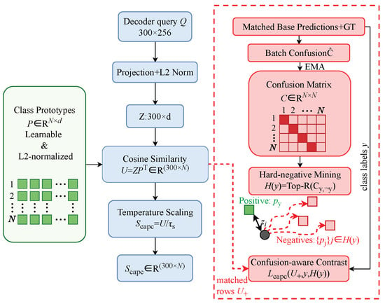
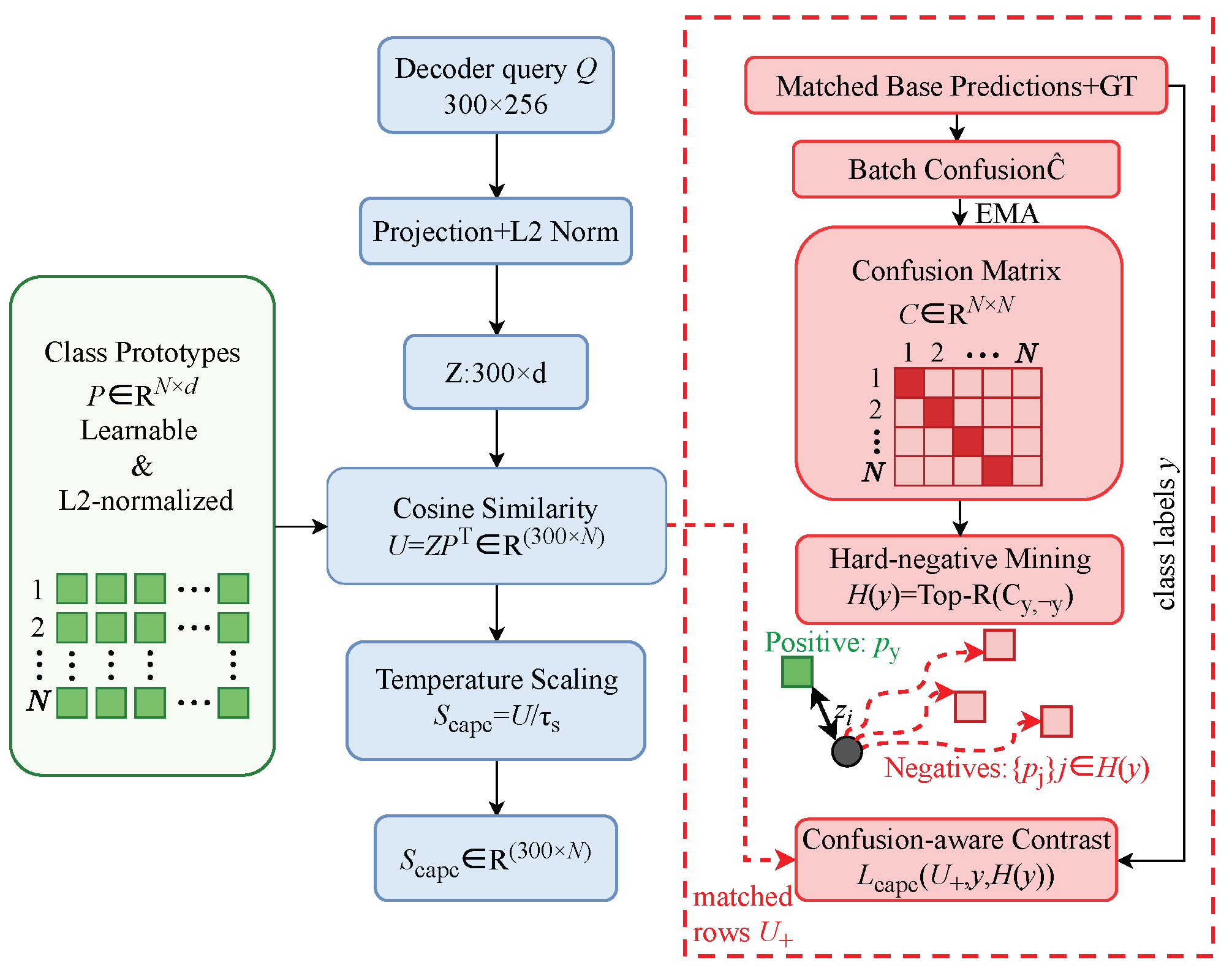
Different types of damage may share similar local textures and edges, making it difficult for a simple linear classification head to explicitly identify the negative classes that are most easily confused with the current class. CAPC retains the base classification head, projects the final Decoder queries into a normalized class-prototype space, and selects hard negative prototypes using confusion relationships accumulated online from the base predictions, as illustrated in Figure 4. The prototype branch of CAPC is retained during both training and inference, whereas matching, the confusion matrix, and the contrastive loss are used only during training.

Figure 4. Structure of CAPC. The class prototypes and query projections on the left jointly produce CAPC classification logits. On the right, only during training, matched base predictions and Ground Truth are used to update an EMA confusion matrix, which is then used to mine hard negative classes for the prototype contrastive loss.

Let ${\mathrm{Proj}}_c(·)$ denote the CAPC query projection head. The query embeddings and learnable class-prototype bank are defined as

$$\begin{array}{cc}\hfill \mathbf{Z}& =\mathrm{L2Norm}\left({\mathrm{Proj}}_c\left(\mathbf{Q}\right)\right)\in {\mathbb{R}}^{300\times d},\hfill \end{array}$$

(16)

$$\begin{array}{cc}\hfill \mathbf{P}& =[{\mathbf{p}}_1;\dots ;{\mathbf{p}}_N]\in {\mathbb{R}}^{N\times d},{\overline{\mathbf{p}}}_c={\displaystyle \frac{{\mathbf{p}}_c}{\parallel {\mathbf{p}}_c{\parallel }_2+\epsilon }}.\hfill \end{array}$$

(17)

The class prototypes are model parameters rather than statistics temporarily generated from a single image or from per-class dataset means. The cosine similarities between queries and prototypes and the temperature-scaled logits are

$$\begin{array}{cc}\hfill \mathbf{U}& =\mathbf{Z}{\overline{\mathbf{P}}}^{\mathsf{T}}\in {\mathbb{R}}^{300\times N},\hfill \end{array}$$

(18)

$$\begin{array}{cc}\hfill {\mathbf{S}}_{\mathrm{capc}}& =\mathbf{U}/{\tau }_s\in {\mathbb{R}}^{300\times N}.\hfill \end{array}$$

(19)

To avoid circular dependence caused by defining hard negative classes using CAPC’s own scores, the confusion statistics are obtained from the matched base-classification predictions. Let ${\mathcal{I}}_c$ denote the set of matched query indices whose Ground Truth class is c in the current batch, and let $p_{\mathrm{base}}(i,j)=\mathrm{sigmoid}\left(S_{\mathrm{base}}(i,j)\right)$. The batch-wise soft confusion matrix is then

$${\widehat{C}}_{cj}={\displaystyle \frac{{\sum }_{i\in {\mathcal{I}}_c}{p}_{\mathrm{base}}(i,j)}{|{\mathcal{I}}_c|+\epsilon }},j\ne c,{\widehat{C}}_{cc}=0.$$

(20)

The confusion matrix $\mathbf{C}\in {\mathbb{R}}^{N\times N}$ is maintained as a gradient-free state and updated using an exponential moving average:

$${\mathbf{C}}^{\left(t\right)}=\mu {\mathbf{C}}^{(t-1)}+(1-\mu ){\widehat{\mathbf{C}}}^{\left(t\right)}.$$

(21)

Given the true class y, its hard negative set is $\mathcal{H}\left(y\right)=\mathrm{error}\{C_{yj}\mid j\ne y\}$. The true label determines only the positive prototype ${\mathbf{p}}_y$, whereas the confusion matrix determines only the set of negative prototypes to be pushed away.

The CAPC auxiliary loss is computed only for foreground queries after Hungarian matching. Let the number of these queries be $K_{+}$ and their true classes be $y_i$; then

$$\begin{array}{cc}\hfill {\mathcal{D}}_i& =\exp (u_{i,y_i}/{\tau }_c)\hfill \\ \hfill & +\sum _{j\in \mathcal{H}\left(y_i\right)}\exp (u_{ij}/{\tau }_c),\hfill \\ \hfill {\mathcal{L}}_{\mathrm{capc}}& =-{\displaystyle \frac{1}{K_{+}}}{\displaystyle \sum _{i=1}^{K_{+}}}\log {\displaystyle \frac{\exp (u_{i,y_i}/{\tau }_c)}{{\mathcal{D}}_i}}.\hfill \end{array}$$

(22)

where ${\tau }_c$ is the temperature for the contrastive loss and is independent of the inference temperature ${\tau }_s$. This loss pulls each query toward the prototype of its true class while pushing it away from the prototypes of the classes with the highest online confusion. Unmatched queries do not participate in this loss, but they still serve as background negatives under the standard classification supervision.

2.5. GAMP: Geometry-Aware Intra-Class Multi-Prototype

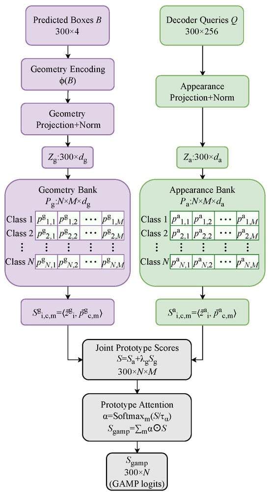
Damage instances of the same class may exhibit different areas, aspect ratios, spatial extents, and texture patterns across different building components and imaging scales. GAMP establishes M paired appearance and geometry prototypes for each class and performs soft selection among intra-class modes according to the query appearance and predicted-box geometry. GAMP receives the final Decoder queries $\mathbf{Q}$ and their corresponding Box Head predictions $\mathbf{B}$. By default, gradients through $\mathbf{B}$ are stopped before it is fed into GAMP to prevent the auxiliary classification loss from interfering with box regression, as illustrated in Figure 5.

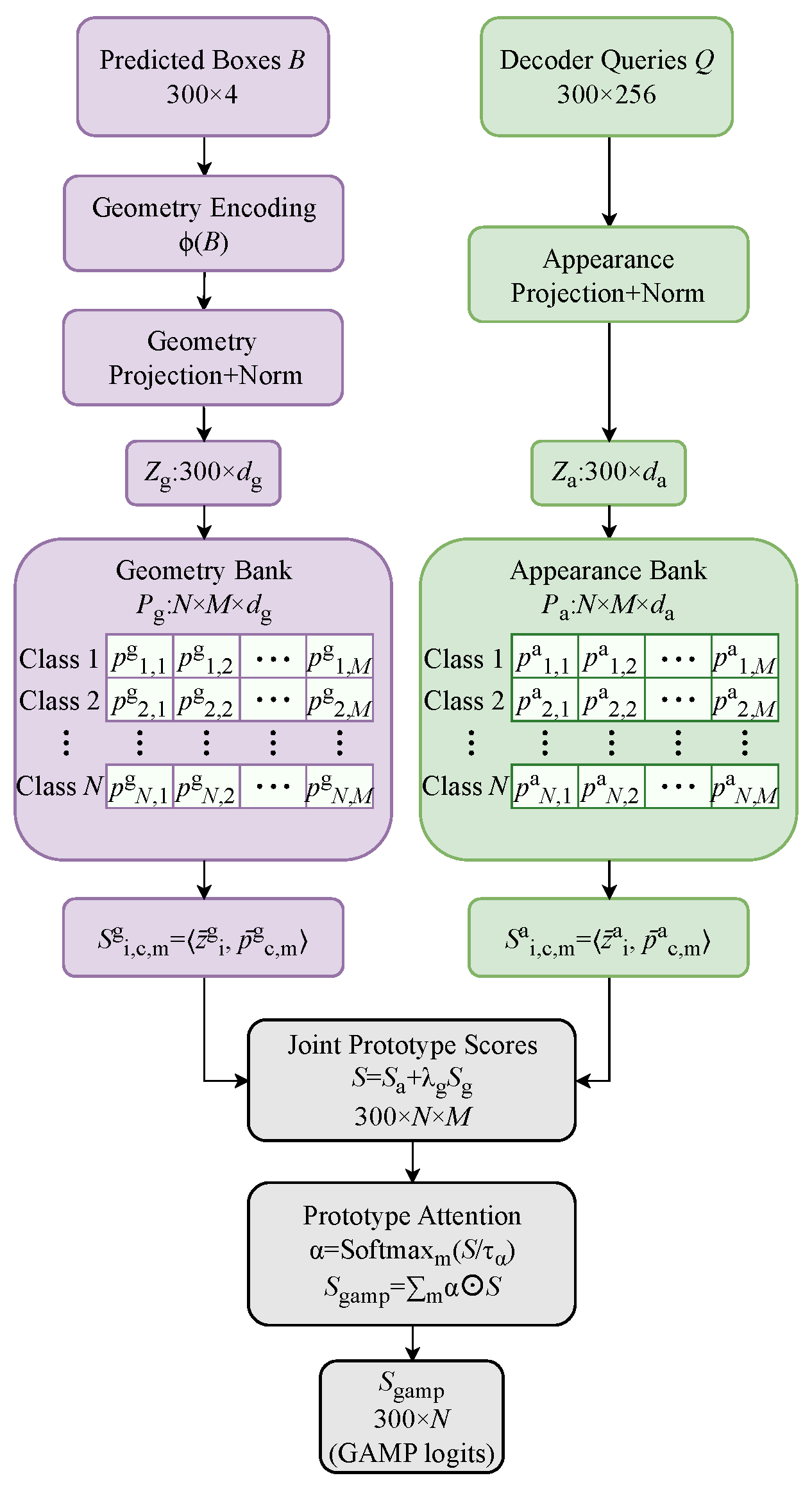
Figure 5. Structure of GAMP. Query appearance and predicted-box geometry are projected into paired appearance/geometry multi-prototype banks, forming joint scores under the same class–mode indices. Prototype Attention aggregates the M modes within each class and outputs ${\mathbf{S}}_{\mathrm{gamp}}$.

The query appearance embedding and the geometric descriptor of the normalized box are defined as

$$\begin{array}{cc}\hfill {\mathbf{Z}}_a& =\mathrm{L2Norm}\left({\mathrm{Proj}}_a\left(\mathbf{Q}\right)\right)\in {\mathbb{R}}^{300\times d_a},\hfill \end{array}$$

(23)

$$\begin{array}{cc}\hfill \mathit{\varphi }\left({\mathbf{b}}_i\right)& =[x_i,y_i,w_i,h_i,w_i{h}_i,w_i/(h_i+\epsilon )],\hfill \end{array}$$

(24)

$$\begin{array}{cc}\hfill {\mathbf{Z}}_g& =\mathrm{L2Norm}\left({\mathrm{Proj}}_g\left(\mathit{\varphi }\left(\mathrm{stopgrad}\left(\mathbf{B}\right)\right)\right)\right)\in {\mathbb{R}}^{300\times d_g}.\hfill \end{array}$$

(25)

The geometric descriptor includes position, scale, area, and aspect ratio, but it is not equivalent to a pixel-level contour, crack topology, or structural-mechanics attribute. GAMP encodes projected box geometry rather than physical dimensions. Increasing camera distance generally reduces projected width, height, and area, whereas oblique views alter aspect ratio and box extent through foreshortening and perspective distortion. Coordinate normalization removes the effect of uniform image resizing but not changes in distance, zoom, or viewpoint. Consequently, the same component can have different geometric descriptors across images. GAMP combines these view-dependent cues with query appearance to select intra-class prototypes; it does not provide camera-pose invariance or metric measurements. Recovering actual component dimensions or damage extent requires additional information, such as camera calibration combined with depth or a known reference scale.

For N classes and M latent modes per class, GAMP establishes two independent prototype banks that are paired under the same $(c,m)$ index:

$${\mathbf{P}}_a\in {\mathbb{R}}^{N\times M\times d_a},{\mathbf{P}}_g\in {\mathbb{R}}^{N\times M\times d_g}.$$

(26)

The mode index m does not correspond to a manually defined subclass; instead, it emerges automatically during training through prototype competition and attention assignment.

The similarities between a query and the paired prototypes, the joint mode score, and the mode attention are respectively defined as

$$\begin{array}{cc}\hfill S_{i,c,m}^a& =⟨{\overline{\mathbf{z}}}_i^a,{\overline{\mathbf{p}}}_{c,m}^a⟩,S_{i,c,m}^g=⟨{\overline{\mathbf{z}}}_i^g,{\overline{\mathbf{p}}}_{c,m}^g⟩,\hfill \end{array}$$

(27)

$$\begin{array}{cc}\hfill S_{i,c,m}& =S_{i,c,m}^a+{\lambda }_g{S}_{i,c,m}^g,\hfill \end{array}$$

(28)

$$\begin{array}{cc}\hfill {\alpha }_{i,c,m}& ={\mathrm{Softmax}}_m(S_{i,c,m}/{\tau }_a),\hfill \end{array}$$

(29)

$$\begin{array}{cc}\hfill S_{\mathrm{gamp}}(i,c)& ={\displaystyle \sum _{m=1}^M}{\alpha }_{i,c,m}{S}_{i,c,m},{\mathbf{S}}_{\mathrm{gamp}}\in {\mathbb{R}}^{300\times N}.\hfill \end{array}$$

(30)

where ${\lambda }_g$ controls the weight of geometric evidence and ${\tau }_a$ controls the sharpness of mode selection. The Softmax is normalized only over the M modes within the same class.

During training, the sample–prototype compactness loss is computed only for matched foreground queries:

$$\begin{array}{cc}\hfill {\mathcal{L}}_{\mathrm{cmp}}& ={\displaystyle \frac{1}{K_{+}}}{\displaystyle \sum _{i=1}^{K_{+}}}{\displaystyle \sum _{m=1}^M}{\alpha }_{i,y_i,m}\hfill \\ \hfill & \times \left[(1-S_{i,y_i,m}^a)+{\lambda }_g(1-S_{i,y_i,m}^g)\right].\hfill \end{array}$$

(31)

To prevent the M prototypes within the same class from collapsing, a cosine-margin diversity constraint is imposed:

$$\begin{array}{cc}\hfill {\rho }_{c,m,n}^r& =\cos ({\mathbf{p}}_{c,m}^r,{\mathbf{p}}_{c,n}^r), r\in \{a,g\},\hfill \\ \hfill {\mathcal{L}}_{\mathrm{div}}& ={\mathrm{Mean}}_{c,m\ne n}[\max (0,{\rho }_{c,m,n}^a-{\delta }_a)\hfill \\ \hfill & +\max (0,{\rho }_{c,m,n}^g-{\delta }_g)].\hfill \end{array}$$

(32)

The GAMP auxiliary constraint can be written as ${\mathcal{L}}_{\mathrm{gamp}}={\lambda }_{\mathrm{cmp}}{\mathcal{L}}_{\mathrm{cmp}}+{\lambda }_{\mathrm{div}}{\mathcal{L}}_{\mathrm{div}}$. During inference, the appearance/geometry projections, paired prototypes, and Prototype Attention are retained, while matching, Ground Truth, and auxiliary losses are not computed. CAPC models inter-class confusion, whereas GAMP models latent intra-class modes; their prototype banks and training constraints are independent of one another.

2.6. Joint Optimization Objective and Inference Procedure

FGCNet follows the one-to-one set matching of RT-DETR, where the matching permutation is jointly determined by the class cost and bounding-box cost. The final-layer classification loss directly supervises the fused ${\mathbf{S}}_{\mathrm{final}}$:

$$\widehat{\sigma }=\underset{\sigma \in {\mathfrak{S}}_K}{\arg \min }\sum _j{\mathcal{C}}_{\mathrm{match}}(y_j,{\mathbf{b}}_j;{\widehat{\mathbf{s}}}_{\sigma \left(j\right)},{\widehat{\mathbf{b}}}_{\sigma \left(j\right)}).$$

(33)

$$\begin{array}{cc}\hfill {\mathcal{L}}_{\det }& ={\mathcal{L}}_{\mathrm{cls}}\left({\mathbf{S}}_{\mathrm{final}}\right)+{\lambda }_{\mathrm{L}1}{\mathcal{L}}_{\mathrm{L}1}\left(\mathbf{B}\right)\hfill \\ \hfill & +{\lambda }_{\mathrm{GIoU}}{\mathcal{L}}_{\mathrm{GIoU}}\left(\mathbf{B}\right)+{\mathcal{L}}_{\mathrm{aux}}+{\mathcal{L}}_{\mathrm{dn}}.\hfill \end{array}$$

(34)

where ${\mathcal{L}}_{\mathrm{aux}}$ and ${\mathcal{L}}_{\mathrm{dn}}$ denote the Decoder auxiliary supervision and contrastive denoising supervision, respectively. Intermediate Decoder layers continue to use the base RT-DETR classification head.

Combining the detection objective and the module-specific constraints, the total loss of FGCNet is

$${\mathcal{L}}_{\mathrm{total}}={\mathcal{L}}_{\det }+{\lambda }_{\mathrm{fg}}{\mathcal{L}}_{\mathrm{fg}}+{\lambda }_{\mathrm{capc}}{\mathcal{L}}_{\mathrm{capc}}+{\lambda }_{\mathrm{cmp}}{\mathcal{L}}_{\mathrm{cmp}}+{\lambda }_{\mathrm{div}}{\mathcal{L}}_{\mathrm{div}}.$$

(35)

All auxiliary losses are used only during training. At the beginning of training, the detection loss and FGWM foreground supervision are enabled. After the matched queries become stable, the CAPC confusion matrix, the CAPC contrastive loss, and the GAMP prototype constraints are gradually activated. The confusion matrix is updated as a gradient-free EMA state, the prototype-loss weights use a warm-up strategy, and M, R, the temperatures, fusion coefficients, and loss weights are determined on the validation set. the fixed fusion coefficients are also selected on this set. The ${\lambda }_{\mathrm{cmp}}$ and ${\lambda }_{\mathrm{div}}$ terms in Equation (35) weight their corresponding constraints only once.

Given a test image, ResNet-50-vd extracts $C_3$–$C_5$ features and projects them to 256 channels. The shared FGWM enhances the three-scale features according to its own predicted ${\mathbf{M}}_{\mathrm{fg}}$. The Hybrid Encoder, Top-K query selection, and six-layer Decoder generate $\mathbf{Q}$ and $\mathbf{B}$. The base classification head then produces ${\mathbf{S}}_{\mathrm{base}}$; CAPC uses the learned class prototypes to produce ${\mathbf{S}}_{\mathrm{capc}}$; and GAMP uses $\mathbf{Q}$, the current predicted boxes, and the learned paired prototypes to produce ${\mathbf{S}}_{\mathrm{gamp}}$. The three sets of logits are fused according to Equation (6). The model directly outputs high-confidence detections corresponding to $({\mathbf{S}}_{\mathrm{final}},\mathbf{B})$ without accessing Ground Truth, updating the confusion matrix, or performing NMS, thereby preserving the end-to-end set-prediction property of RT-DETR.

3. Experimental Results and Analysis

3.1. Datasets and Experimental Settings

(1) Dataset: To verify the effectiveness of the proposed method in real urban landscape building damage scenarios, we construct an urban landscape building damage dataset. The dataset contains 1000 images with resolutions of $3872\times 2592$ or $2592\times 3872$ pixels, all acquired with a professional handheld camera. The data cover a variety of real scenes, including indoor spaces, outdoor environments, corridors, and building facades, and include building components and damaged regions under different shooting distances, viewpoints, illumination conditions, and complex backgrounds. Unlike datasets focusing on a single material or a single damage form, this dataset deliberately preserves variations in building structure, scale, texture, and spatial location found in real urban landscape environments in order to evaluate the applicability and robustness of detection models under complex scenes.

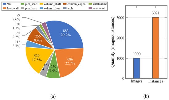
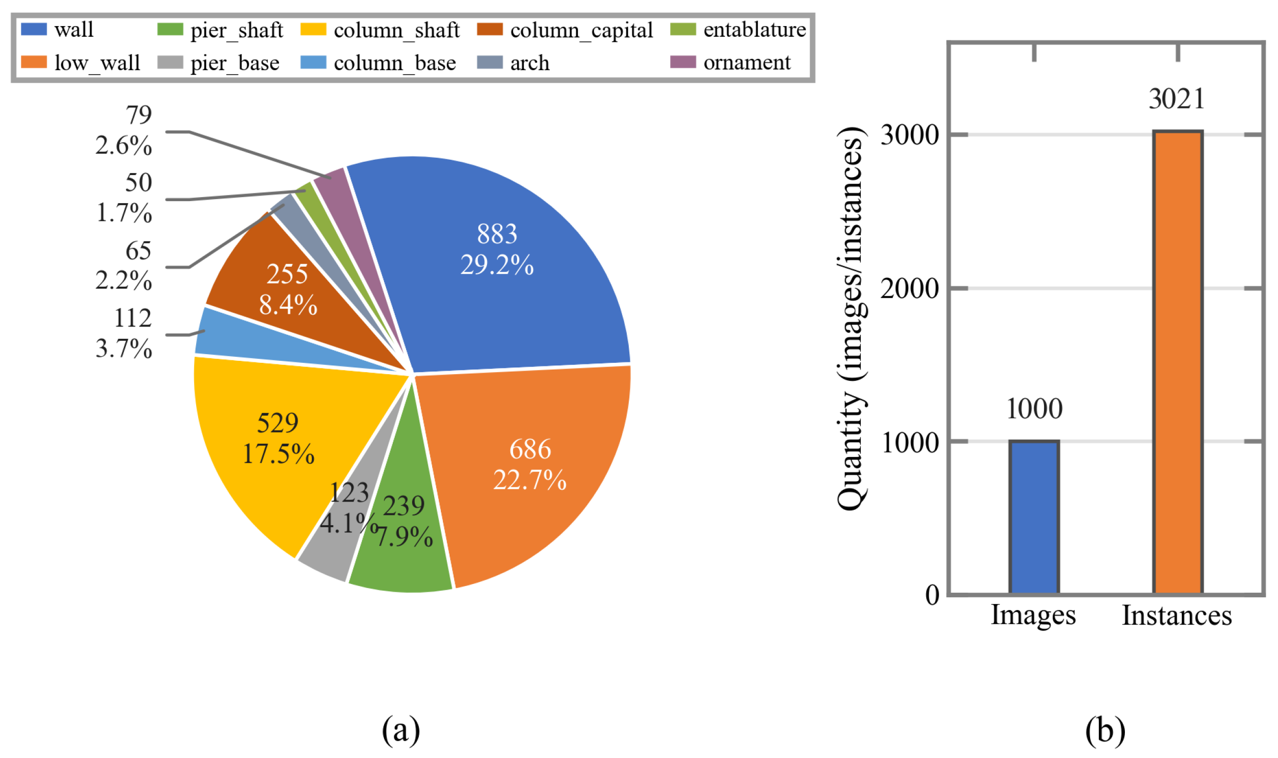
Because building damage is typically associated with different structural locations, and because structural shape, scale, and surface texture directly affect the visual appearance of damaged regions, the categories in this study are defined according to the building structure on which the damage occurs rather than by further distinguishing component materials. The dataset contains 10 categories of damaged components: wall, low_wall, pier_shaft, pier_base, column_shaft, column_base, column_capital, arch, entablature, and ornament. As shown in Figure 6a, these categories contain 883, 686, 239, 123, 529, 112, 255, 65, 50, and 79 annotated bounding-box instances, respectively, for a total of 3021 annotated instances. The overall dataset scale is shown in Figure 6.

Figure 6. Category distribution and overall scale of the urban landscape building damage dataset. (a) Number of annotated instances for each category. (b) Overall dataset scale.

The class distribution shows that wall and low_wall account for 29.2% and 22.7% of all annotated instances, respectively, whereas categories such as ornament, arch, and entablature contain relatively few samples, indicating a certain degree of class imbalance. This natural frequency distribution was retained; limited samples for rare classes remain a dataset limitation to be addressed through targeted future collection. There are also clear scale differences between components: walls and low walls generally occupy large visible regions, whereas local components such as column bases and ornaments occupy relatively small pixel areas. In addition, occlusion, perspective deformation, complex decorative textures, and illumination and shadow variations further increase the difficulty of localizing damaged regions and determining their categories. Thus, the dataset reflects several important challenges in real urban landscape building damage detection, including complex backgrounds, inter-class visual similarity, and intra-class morphological variation.

For data annotation, LabelImg was used to manually annotate the building-component regions containing damage with bounding boxes, and category labels were created according to the 10 structural classes described above. The 1000 images were divided by physical building into training, validation, and test sets at a ratio of 7:2:1 (700, 200, and 100 images, respectively). Images of different facades or viewpoints of the same building remain in the same set, so no building is shared across sets. The training set is used to learn model parameters, the validation set for model selection and hyperparameter tuning, and the independent test set only for final performance evaluation.

(2) Experimental Settings: All models were trained or tested under the same software and hardware environment to ensure fair comparisons among different methods. Python 3.10 was used as the programming language, and the experiments were implemented using the PyTorch 2.3.1 deep-learning framework. The operating system was Linux, with an NVIDIA RTX3090 GPU, an Intel Core i7-12700H CPU, 64 GB of RAM, and CUDA 12.2. The training settings are an input image size of $640\times 640$, batch size of 4, 300 epochs, an initial learning rate of 0.005 decayed by a factor of 0.01, and the AdamW optimizer. The detailed experimental environment is listed in Table 1. Except for differences inherent to the model architectures, all comparison experiments used the same dataset and evaluation configuration for performance statistics.

Table 1. Hardware and software configurations.

Configuration	Model Number/Version
Programming language	Python
Deep learning framework	PyTorch
Operating system	Linux
GPU	NVIDIA RTX3090
CPU	Intel Core i7-12700H
RAM	64 GB
CUDA	12.2

3.2. Evaluation Metrics

To comprehensively evaluate the classification and localization performance of the models on the urban landscape building damage detection task, Precision (P), Recall (R), Average Precision (AP), mean Average Precision (mAP), Average Recall (AR), and Frames Per Second (FPS) are used as evaluation metrics. P and R, respectively, reflect the accuracy of the predictions and the model’s ability to detect Ground Truth targets and are calculated as

$$P={\displaystyle \frac{TP}{TP+FP}},$$

(36)

$$R={\displaystyle \frac{TP}{TP+FN}},$$

(37)

where $TP$ denotes the number of correctly detected targets, $FP$ denotes the number of incorrect predictions, and $FN$ denotes the number of Ground Truth targets that are not detected.

To further measure overall detection performance under different confidence thresholds, AP is calculated from the Precision–Recall curve as

$$AP={\displaystyle \sum _{i=1}^N}P\left(i\right)\Delta R\left(i\right),$$

(38)

where $P\left(i\right)$ is the Precision at the ith recall position, and $\Delta R\left(i\right)$ denotes the change in Recall between adjacent thresholds. For a dataset containing C classes, mAP is defined as the mean AP over all classes:

$$mAP={\displaystyle \frac{1}{C}}{\displaystyle \sum _{c=1}^C}A{P}_c.$$

(39)

We report ${\mathrm{mAP}}_{50}$, ${\mathrm{mAP}}_{75}$, and ${\mathrm{mAP}}_{50:95}$. Here, ${\mathrm{mAP}}_{50}$ and ${\mathrm{mAP}}_{75}$ denote mean Average Precision at IoU thresholds of 0.50 and 0.75, respectively, while ${\mathrm{mAP}}_{50:95}$ is averaged over IoU thresholds from 0.50 to 0.95 with a step size of 0.05. To measure target coverage, ${\mathrm{AR}}_1$ and ${\mathrm{AR}}_{100}$ are also reported, representing Average Recall when at most 1 and 100 detections per image are retained, respectively. FPS is used to measure inference speed, with a higher value indicating stronger real-time detection capability.

3.3. Comparisons with State-of-the-Art Methods

To verify the effectiveness of the proposed method, we compare it on the urban landscape building damage dataset with several representative object detectors, including Cascade R-CNN [22], RetinaNet [23], Grid R-CNN [24], Dynamic R-CNN [25], Sparse R-CNN [26], TOOD [27], RTMDet [28], YOLOv5s, YOLOv8s [29], YOLOv9s [30], and YOLOv10s [31]. The class-wise comparison additionally includes YOLOv11s [32] and YOLOv12s [33]. RT-DETR is used as the baseline model, while the complete proposed model is denoted as FGCNet. To analyze performance from different perspectives, we report the class-wise ${\mathrm{AP}}_{50}$ for each damaged-component category, together with the overall metrics ${\mathrm{mAP}}_{50:95}$, ${\mathrm{mAP}}_{50}$, ${\mathrm{mAP}}_{75}$, ${\mathrm{AR}}_1$, ${\mathrm{AR}}_{100}$, and FPS. The results are presented in Table 2 and Table 3, respectively.

Table 2. Class-wise detection performance comparison on the urban landscape building damage dataset.

Method	${\mathit{AP}}_{50}$ Wall	${\mathit{AP}}_{50}$ Low Wall	${\mathit{AP}}_{50}$ Pier Shaft	${\mathit{AP}}_{50}$ Pier Base	${\mathit{AP}}_{50}$ Column Shaft	${\mathit{AP}}_{50}$ Column Base	${\mathit{AP}}_{50}$ Column Capital	${\mathit{AP}}_{50}$ Arch	${\mathit{AP}}_{50}$ Entablature	${\mathit{AP}}_{50}$ Ornament
Cascade R-CNN	37.5	19.4	13.3	71.9	42.5	42.8	19.8	18.1	58.4	34.4
RetinaNet	27.8	22.8	19.0	58.0	38.5	31.5	22.5	20.1	44.0	27.5
Grid R-CNN	44.4	36.8	15.6	73.9	39.2	36.2	22.6	11.9	50.5	42.8
Dynamic R-CNN	42.7	33.3	13.4	80.5	46.9	38.4	31.4	16.6	58.6	44.6
Sparse R-CNN	34.9	21.8	12.9	77.2	42.1	42.8	23.1	20.2	59.6	35.6
TOOD	51.7	39.6	19.0	82.1	44.1	36.0	26.3	14.7	55.3	48.2
RTMDet	49.4	43.3	41.8	73.5	50.1	43.3	31.9	22.3	57.8	45.6
YOLOv5s	44.5	35.2	14.3	80.5	46.1	36.7	29.9	17.2	56.0	46.8
YOLOv8s	47.0	36.9	16.9	81.0	47.1	40.9	31.6	17.6	57.9	49.1
YOLOv9s	46.8	37.2	18.4	81.4	49.8	42.2	34.4	18.0	62.6	49.9
YOLOv10s	49.1	38.0	19.3	82.5	50.0	44.5	34.5	18.4	65.6	51.9
YOLOv11s	50.6	39.2	19.8	83.1	50.7	43.9	35.2	18.9	64.7	52.6
YOLOv12s	51.4	40.1	20.4	83.8	51.3	45.0	35.8	19.2	66.3	53.2
RT-DETR (Baseline)	53.3	42.8	16.9	84.6	49.4	38.8	30.5	19.8	56.7	52.5
FGCNet (Ours)	56.1	46.0	20.7	85.8	52.9	41.7	35.4	20.6	66.1	57.0

Note: All AP values are reported in %; bold values indicate the best result in each category.

Table 3. Overall detection performance comparison on the urban landscape building damage dataset.

Method	${\mathbf{mAP}}_{50:95}$	${\mathbf{mAP}}_{50}$	${\mathbf{mAP}}_{75}$	${\mathbf{AR}}_1$	${\mathbf{AR}}_{100}$	FPS
Cascade R-CNN	25.6	35.8	26.8	18.9	34.7	49.0
RetinaNet	27.7	31.2	29.1	19.8	35.9	59.3
Grid R-CNN	26.2	37.4	27.0	19.0	35.2	47.5
Dynamic R-CNN	25.9	40.6	25.7	18.6	34.8	46.8
Sparse R-CNN	28.2	37.0	29.3	20.5	37.2	32.7
TOOD	21.4	41.7	20.6	15.8	30.1	48.9
RTMDet	28.2	45.9	28.8	20.3	37.6	47.6
YOLOv5s	24.0	40.7	23.7	17.6	33.3	44.6
YOLOv8s	25.6	42.6	25.4	18.7	35.1	44.6
YOLOv9s	27.1	44.1	27.4	19.7	36.5	45.9
YOLOv10s	28.0	45.4	28.4	20.2	37.4	48.2
RT-DETR (Baseline)	28.2	44.5	28.5	19.7	36.8	78.3
FGCNet (Ours)	30.8	48.2	31.7	22.4	40.6	68.2

Note: Detection metrics are reported in %, except FPS; bold values indicate the best result.

The class-wise ${\mathrm{AP}}_{50}$ results reveal clear differences in detection difficulty among building components. FGCNet achieves the best result in 7 of the 10 categories: wall, low_wall, pier_base, column_shaft, column_capital, entablature, and ornament. Compared specifically with YOLOv12s, it has higher ${\mathrm{AP}}_{50}$ in 7 of the 10 categories. The ${\mathrm{AP}}_{50}$ for pier_base reaches 85.8%, making it the best-performing category for the proposed method; entablature, ornament, wall, and column_shaft achieve 66.1%, 57.0%, 56.1%, and 52.9%, respectively. These categories generally have relatively stable structural outlines or distinctive local-region characteristics, enabling the model to produce more reliable localization and classification results. In contrast, FGCNet obtains ${\mathrm{AP}}_{50}$ values of 20.7% and 20.6% for pier_shaft and arch, respectively, indicating that these two categories remain difficult in the current dataset.

Compared with the baseline, FGCNet achieves positive improvements in all 10 categories. The gains for wall, low_wall, pier_shaft, pier_base, column_shaft, column_base, column_capital, arch, entablature, and ornament are 2.8, 3.2, 3.8, 1.2, 3.5, 2.9, 4.9, 0.8, 9.4, and 4.5 percentage points, respectively. The largest gain is observed for entablature, reaching 9.4 percentage points, while column_capital and ornament improve by 4.9 and 4.5 percentage points, respectively. These results indicate that the performance gains of the proposed method do not arise solely from a small number of easy-to-detect classes but extend across multiple damaged-component categories with different scales, textures, and morphologies.

It should be noted that the proposed method does not achieve the best performance in every category. RTMDet obtains ${\mathrm{AP}}_{50}$ values of 41.8% and 22.3% for pier_shaft and arch, respectively, both higher than those of FGCNet. YOLOv12s achieves the best result of 45.0% for column_base, whereas FGCNet obtains 41.7%. YOLOv12s also scores 35.8% for column_capital, compared with 35.4% for FGCNet. In particular, RTMDet performs substantially better than the other models on pier_shaft, indicating that different detectors still vary in their ability to model specific scales, textures, or geometric structures.

FGCNet trails RTMDet by 21.1 percentage points for pier_shaft and 1.7 for arch. These categories contain 239 and 65 instances, respectively, although sample count alone cannot explain the performance gap. Visual similarity between pier_shaft and other vertical components can complicate classification under occlusion and perspective changes, while curved boundaries and repeated neighboring structures can make arch localization ambiguous. FGWM uses rectangular foreground supervision that may include background, and GAMP describes box geometry without explicitly modeling contours or structural relationships. These representations may therefore be insufficient to distinguish similar vertical components or capture arch shapes. Despite improving over RT-DETR by 3.8 and 0.8 percentage points, respectively, FGCNet retains these category-specific weaknesses.

In terms of overall detection performance, FGCNet achieves the best results on all five accuracy and recall metrics, namely, ${\mathrm{mAP}}_{50:95}$, ${\mathrm{mAP}}_{50}$, ${\mathrm{mAP}}_{75}$, ${\mathrm{AR}}_1$, and ${\mathrm{AR}}_{100}$, reaching 30.8%, 48.2%, 31.7%, 22.4%, and 40.6%, respectively. Compared with the baseline, ${\mathrm{mAP}}_{50:95}$ increases from 28.2% to 30.8%, a gain of 2.6 percentage points; ${\mathrm{mAP}}_{50}$ increases from 44.5% to 48.2%, a gain of 3.7 percentage points; and ${\mathrm{mAP}}_{75}$ increases from 28.5% to 31.7%, a gain of 3.2 percentage points. Notably, the improvement in ${\mathrm{mAP}}_{75}$ remains clear under the stricter IoU threshold, indicating that the proposed method improves not only target detection but also bounding-box localization quality.

For recall performance, FGCNet improves ${\mathrm{AR}}_1$ from 19.7% to 22.4% and ${\mathrm{AR}}_{100}$ from 36.8% to 40.6%, corresponding to gains of 2.7 and 3.8 percentage points, respectively. The increase in ${\mathrm{AR}}_1$ indicates that the model can more accurately identify key targets when only a small number of high-confidence predictions are retained. The improvement in ${\mathrm{AR}}_{100}$ shows that, when more candidate boxes are allowed, the model further improves its coverage of targets across different classes and scales. Thus, the overall improvement of the proposed method is reflected in both localization accuracy and missed-detection suppression.

Among the remaining comparison methods, RTMDet and Sparse R-CNN both achieve ${\mathrm{mAP}}_{50:95}=28.2\%$, the highest result apart from FGCNet; FGCNet improves this value by 2.6 percentage points. For ${\mathrm{mAP}}_{50}$, RTMDet obtains 45.9%, while FGCNet further improves it by 2.3 percentage points. For ${\mathrm{mAP}}_{75}$, Sparse R-CNN ranks first among the other comparison methods at 29.3%, whereas FGCNet remains 2.4 percentage points higher. Regarding recall, Sparse R-CNN achieves ${\mathrm{AR}}_1=20.5\%$ and RTMDet achieves ${\mathrm{AR}}_{100}=37.6\%$, while FGCNet reaches 22.4% and 40.6%, respectively. These results demonstrate that the proposed method maintains a relatively stable overall advantage over different types of detectors.

In terms of inference efficiency, the baseline model achieves the highest speed at 78.3 FPS, whereas FGCNet runs at 68.2 FPS. After introducing the proposed modules, FGCNet decreases by 10.1 FPS relative to the baseline, corresponding to a reduction of approximately 12.9%, indicating that the performance improvement incurs additional computational overhead. Nevertheless, FGCNet remains faster than all other comparison models. RetinaNet, the fastest model apart from the baseline, reaches 59.3 FPS, while FGCNet is 8.9 FPS faster. Therefore, under the current experimental platform and evaluation configuration, the proposed method retains good real-time detection performance while improving detection accuracy and recall.

The additional complexity comparison in Table 4 shows that FGCNet adds 1.60 M parameters and 3.6 G FLOPs relative to RT-DETR at $640\times 640$ input resolution. YOLOv12s is smaller and has fewer FLOPs, while its measured speed is 46.30 FPS under the reported evaluation setup.

Table 4. Model complexity and inference speed at an input size of $640\times 640$.

Model	Parameters (M)	FLOPs (G)	FPS
RT-DETR	32.15	103.8	78.30
FGCNet	33.75	107.4	68.24
YOLOv12s	9.26	23.2	46.30

RT-DETR and FGCNet were each repeated with five training seeds (0, 42, 2025, 2026, and 1248). Table 5 and Table 6 report the mean, standard deviation, and individual results. Across seeds, FGCNet improves mean ${\mathrm{mAP}}_{50}$ by 3.73 percentage points, with standard deviations of 0.37 and 0.44 percentage points for RT-DETR and FGCNet, respectively.

Table 5. Five-seed results: mean, standard deviation (SD), and mean difference. All detection metrics and differences are in percentage points; FPS is in frames/s.

Metric	RT-DETR Mean	RT-DETR SD	FGCNet Mean	FGCNet SD	Difference
Precision	51.59	0.32	54.50	0.35	+2.91
Recall	43.80	0.29	46.71	0.30	+2.91
${\mathrm{mAP}}_{50:95}$	28.22	0.21	30.81	0.30	+2.59
${\mathrm{mAP}}_{50}$	44.53	0.37	48.26	0.44	+3.73
${\mathrm{mAP}}_{75}$	28.50	0.34	31.70	0.34	+3.20
${\mathrm{AR}}_1$	19.71	0.30	22.42	0.34	+2.71
${\mathrm{AR}}_{100}$	36.81	0.38	40.60	0.38	+3.79
FPS	78.30	0.16	68.24	0.21	−10.06

Table 6. Results of individual training seeds. Detection metrics are in %; FPS is in frames/s.

Model	Seed	Precision	Recall	${\mathbf{mAP}}_{50:95}$	${\mathbf{mAP}}_{50}$	${\mathbf{mAP}}_{75}$	${\mathbf{AR}}_1$	${\mathbf{AR}}_{100}$	FPS
RT-DETR	0	51.17	43.52	28.10	44.16	28.11	19.38	36.33	78.1
RT-DETR	42	51.88	43.91	28.38	44.72	28.76	19.95	37.08	78.5
RT-DETR	2025	51.42	43.82	28.17	44.31	28.36	19.57	36.81	78.2
RT-DETR	2026	51.94	44.21	28.49	45.08	28.95	20.09	37.27	78.3
RT-DETR	1248	51.54	43.54	27.96	44.38	28.32	19.56	36.56	78.4
FGCNet	0	54.03	46.34	30.46	47.74	31.22	21.94	40.05	68.0
FGCNet	42	54.74	46.89	31.08	48.61	31.97	22.67	40.84	68.5
FGCNet	2025	54.47	46.57	30.64	48.02	31.53	22.25	40.62	68.1
FGCNet	2026	54.93	47.11	31.16	48.82	32.06	22.78	41.03	68.4
FGCNet	1248	54.31	46.66	30.73	48.12	31.72	22.46	40.46	68.2

Taken together, the class-wise and overall results show that FGCNet not only achieves the best overall $\mathrm{mAP}$ and $\mathrm{AR}$ metrics but also obtains the highest ${\mathrm{AP}}_{50}$ in 5 of the 10 categories and improves over the baseline in every category. This indicates that the overall performance gain has a broad class basis rather than being driven by a single easy-to-detect category. At the same time, pier_shaft, column_base, and arch still leave room for further improvement, suggesting that complex textures, local scale variation, and fine-grained discrimination between similar structures remain important challenges for future work.

To validate the superiority of our proposed wavelet-based FGWM over existing wavelet-based approaches, we further compare FGWM with three representative wavelet-based modules, namely, WTConv [34], HWAB [35], and WAT [36]. For a fair comparison, all modules are evaluated using the same baseline architecture and evaluation protocol. The corresponding results are reported in Table 7.

Table 7. Performance comparison of FGWM and alternative wavelet modules on the urban landscape building damage dataset.

Model	Precision	Recall	${\mathbf{mAP}}_{50:95}$	${\mathbf{mAP}}_{50}$
Baseline	51.6	43.8	28.2	44.5
Baseline+WTConv [34]	51.8	42.6	28.3	45.2
Baseline+HWAB [35]	52.4	43.2	27.8	44.5
Baseline+WAT [36]	51.8	43.4	28.5	45.4
Baseline+FGWM	52.1	44.9	29.0	45.9

Note: All metric values are reported in %; bold values indicate the best result.

Compared with the baseline, the alternative wavelet modules yield mixed changes across the four metrics. WTConv improves Precision, ${\mathrm{mAP}}_{50:95}$, and ${\mathrm{mAP}}_{50}$ by 0.2, 0.1, and 0.7%, respectively, but decreases Recall by 1.2%. HWAB achieves the highest Precision of 52.4%, whereas its Recall and ${\mathrm{mAP}}_{50:95}$ are 0.6% and 0.4% below the baseline, respectively. The FGWM provides the strongest AP results among the three alternative modules, reaching 29.0% ${\mathrm{mAP}}_{50:95}$ and 45.9% ${\mathrm{mAP}}_{50}$. This indicates that FGWM can effectively improve the detection performance of RT-DETR in terms of both precision and recall. In contrast, FGWM achieves a more favorable balance between prediction reliability and target coverage. This indicates that FGWM does not uniformly enhance frequency-domain responses; instead, it leverages foreground–background contrast statistics to generate subband-specific modulation.

3.4. Visual Comparison of Different Model Detection Results

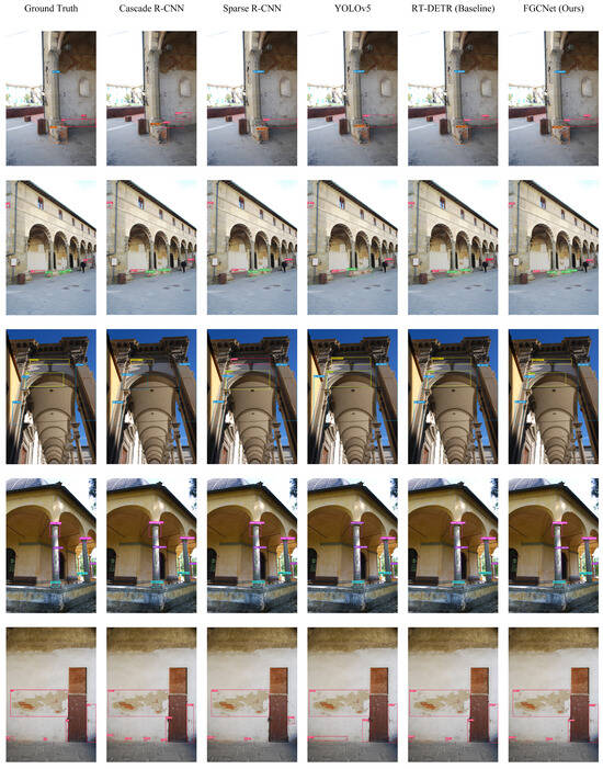
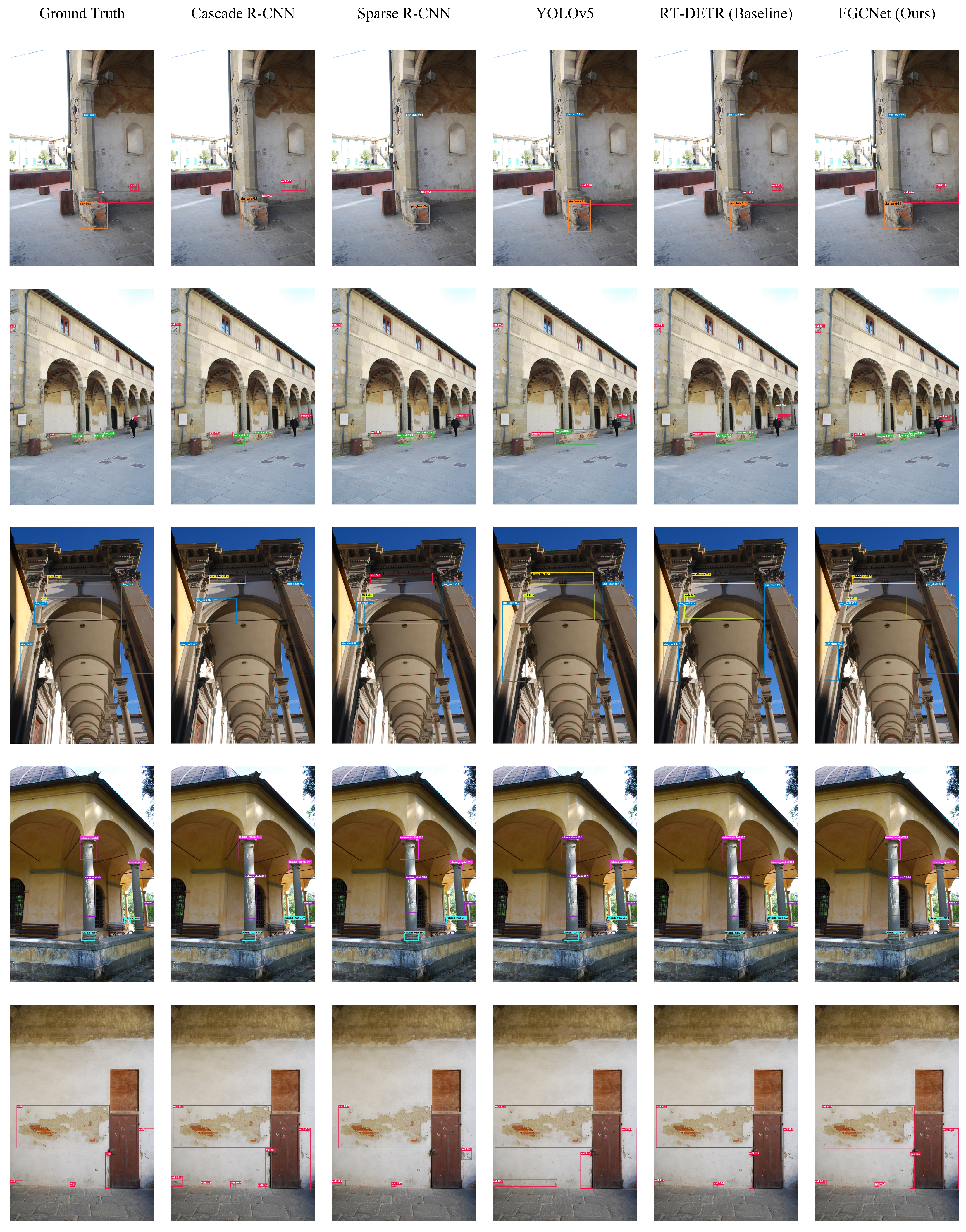
To visually examine the detection differences among different models in real urban landscape building scenes, representative samples are selected from the test set, and FGCNet is compared with Cascade R-CNN, Sparse R-CNN, YOLOv5, and the baseline. The results are shown in Figure 7. The selected samples cover different architectural scenes, including walls, corridors, arches, column components, and large-area finishes, and include cases with multiple coexisting targets, repeated structural textures, scale variations, and background interference.

Figure 7. Visual comparison of different detection models on the urban landscape building damage dataset. From left to right: Ground Truth, Cascade R-CNN, Sparse R-CNN, YOLOv5, RT-DETR (Baseline), and FGCNet (Ours).

As shown in Figure 7, the predictions of FGCNet are generally more consistent with the Ground Truth and are more stable in terms of target count, class determination, and bounding-box spatial extent. By comparison, Cascade R-CNN and Sparse R-CNN produce redundant predictions, missed targets, or inaccurate box extents in some scenes. YOLOv5 and the baseline also exhibit localization offsets or incomplete detections when complex textures, small local components, and multiple adjacent targets occur simultaneously. FGCNet maintains more complete target responses across different viewpoints and structural scales. In particular, for repeated arches, slender column components, and large wall damage regions, the correspondence between predicted boxes and the Ground Truth regions is more stable. These visualization results are consistent with the quantitative results in Table 2 and Table 3, demonstrating that the proposed method improves the identification and localization quality of damaged components under complex urban landscape backgrounds.

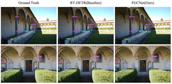
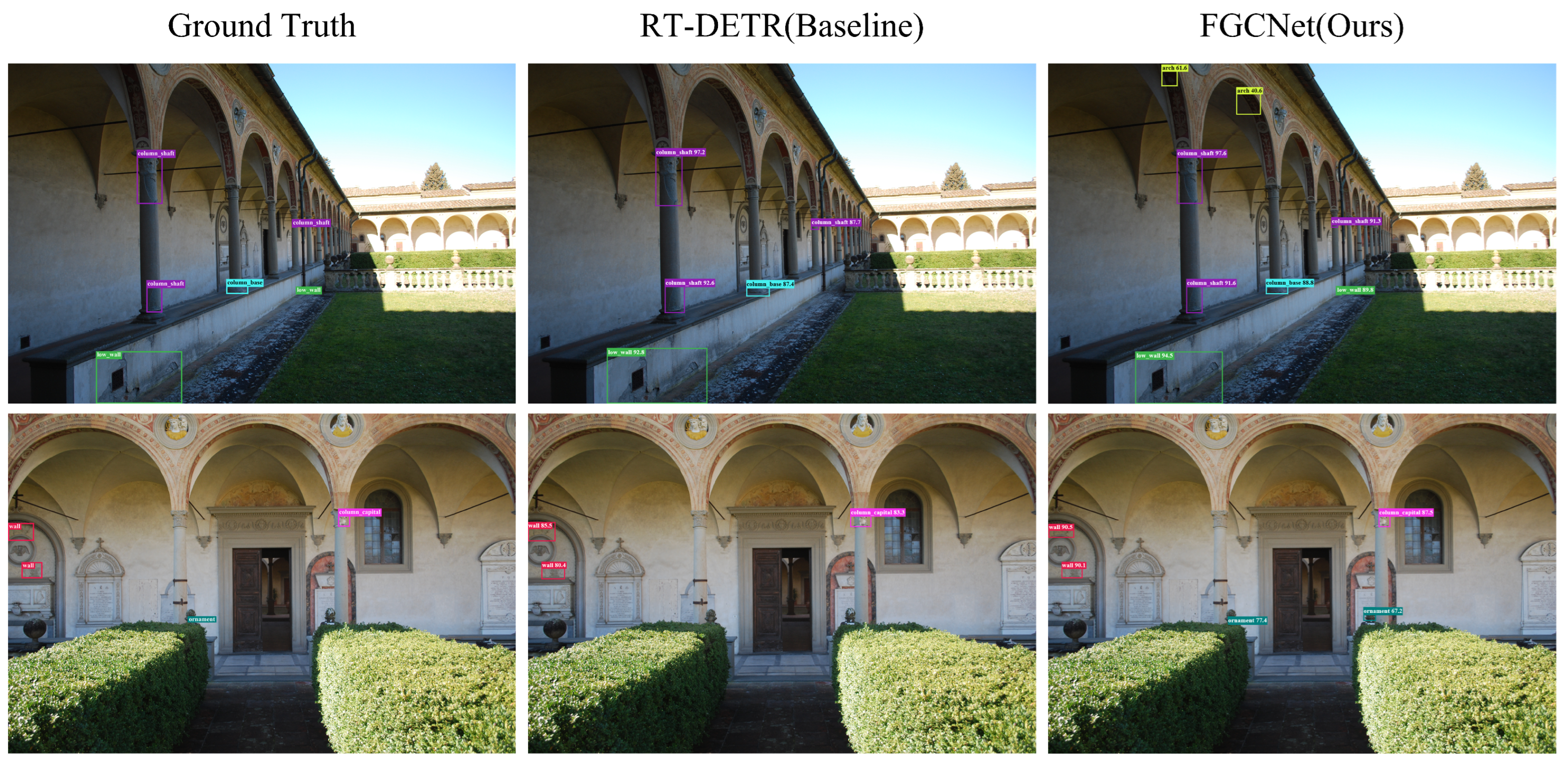
Figure 8 shows two failure cases. In the first row, FGCNet detects most column and low-wall targets but falsely predicts an arch in a decorated region under strong illumination variation. In the second row, ornament-like textures and vegetation occlusion cause extra predictions despite improved target response. Similar textures and geometry, shadows, occlusion, and scarce arch samples remain challenges.

Figure 8. Typical failure cases of FGCNet on the urban landscape building damage dataset. From left to right: Ground Truth, RT-DETR (Baseline), and FGCNet (Ours).

3.5. Ablation Experiments

To verify the independent contributions and complementary effects of FGWM, CAPC, and GAMP, ablation experiments are conducted under the same dataset and experimental configuration. Precision, Recall, ${\mathrm{mAP}}_{50:95}$, and ${\mathrm{mAP}}_{50}$ are compared by introducing each individual module, all pairwise module combinations, and the complete combination of all three modules. The results are shown in Table 8.

Table 8. Detection performance comparison using different components on the urban landscape building damage dataset.

Model	FGWM	CAPC	GAMP	Precision	Recall	${\mathbf{mAP}}_{50:95}$	${\mathbf{mAP}}_{50}$
Baseline				51.6	43.8	28.2	44.5
Baseline	✓			52.1	44.9	29.0	45.9
Baseline		✓		52.8	43.6	28.9	45.7
Baseline			✓	52.3	44.7	28.8	45.6
Baseline	✓	✓		53.4	45.1	29.7	46.8
Baseline		✓	✓	52.9	46.1	29.9	47.1
Baseline	✓		✓	53.6	45.5	30.0	47.3
Baseline	✓	✓	✓	54.5	46.7	30.8	48.2

Note: A checkmark indicates that the corresponding component is included in the model, while a blank cell indicates that it is not included. All metric values are reported in %; bold values indicate the best result.

As shown in Table 8, the baseline achieves Precision, Recall, ${\mathrm{mAP}}_{50:95}$, and ${\mathrm{mAP}}_{50}$ values of 51.6%, 43.8%, 28.2%, and 44.5%, respectively. Introducing FGWM alone increases Recall by 1.1 percentage points and improves ${\mathrm{mAP}}_{50:95}$ and ${\mathrm{mAP}}_{50}$ by 0.8 and 1.4 percentage points, respectively. This indicates that foreground-guided wavelet modulation can strengthen edge and texture responses in weakly damaged regions and reduce interference from complex backgrounds and illumination changes during feature extraction.

Introducing CAPC alone increases Precision from 51.6% to 52.8%, a gain of 1.2 percentage points, while Recall decreases slightly from 43.8% to 43.6%. This overall result is consistent with the intended role of CAPC, but it does not by itself establish a reduction in confusion between any specific pair of classes. Introducing GAMP alone increases Recall by 0.9 percentage points and improves ${\mathrm{mAP}}_{50:95}$ and ${\mathrm{mAP}}_{50}$ by 0.6 and 1.1 percentage points, respectively, showing that geometry-aware intra-class multi-prototype modeling helps describe variations in scale, aspect ratio, and morphology within the same class.

For two-module combinations, using FGWM and CAPC together improves Precision, Recall, ${\mathrm{mAP}}_{50:95}$, and ${\mathrm{mAP}}_{50}$ by 1.8, 1.3, 1.5, and 2.3 percentage points, respectively. Combining CAPC and GAMP increases Recall by 2.3 percentage points and raises ${\mathrm{mAP}}_{50}$ to 47.1%. Combining FGWM and GAMP achieves a Precision of 53.6% and an ${\mathrm{mAP}}_{50}$ of 47.3%. These results show that the modules improve feature representation from complementary perspectives, including foreground-detail enhancement, inter-class discrimination, and modeling of intra-class geometric variation.

When FGWM, CAPC, and GAMP are all introduced, the complete FGCNet achieves the best results. Precision and Recall reach 54.5% and 46.7%, respectively, both 2.9 percentage points higher than the baseline; ${\mathrm{mAP}}_{50:95}$ and ${\mathrm{mAP}}_{50}$ reach 30.8% and 48.2%, corresponding to gains of 2.6 and 3.7 percentage points. These results show that the joint use of the three modules effectively combines local damage-detail enhancement, separation of visually similar classes, and modeling of geometric variations within the same class, thereby producing more stable representations of building damage.

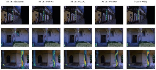
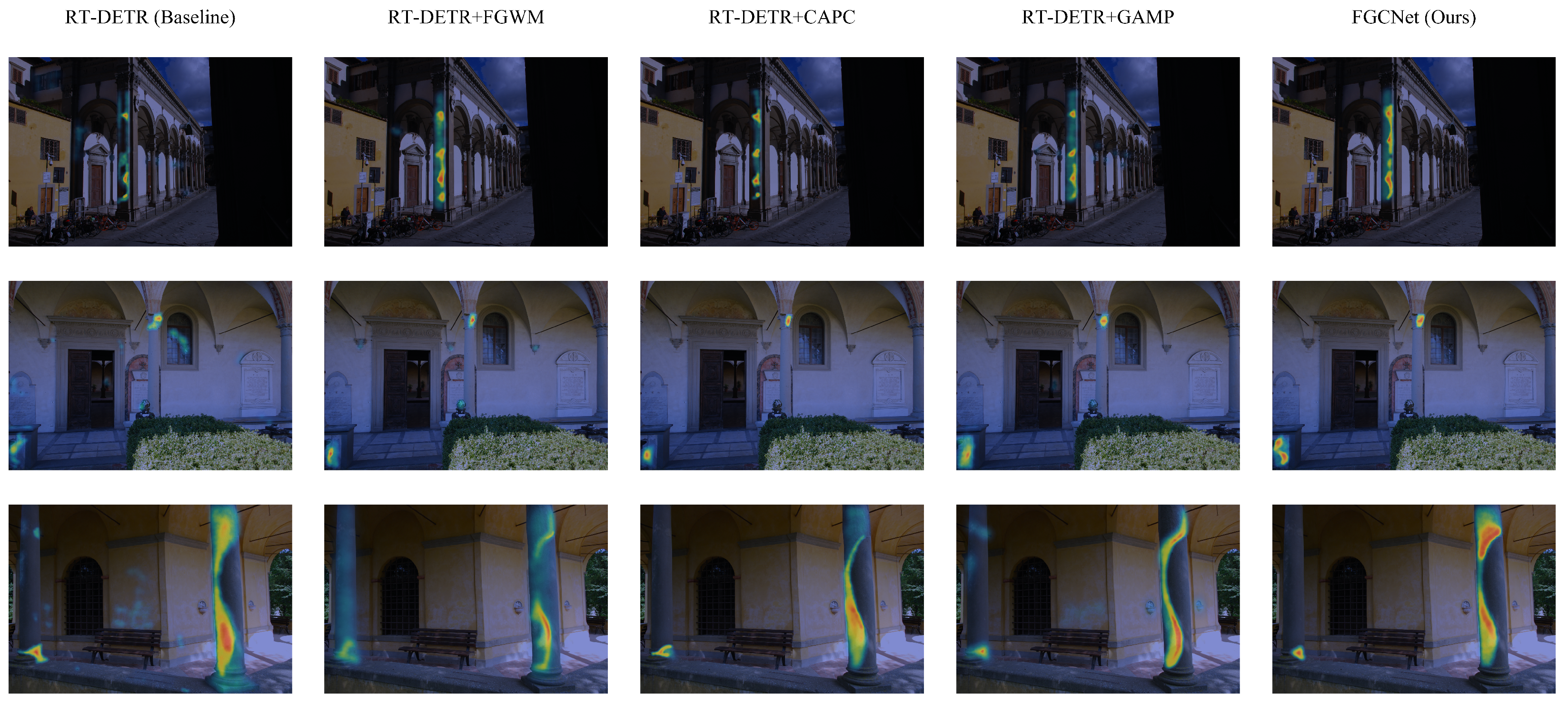
To further analyze the independent effects and combined behavior of the three modules at the feature-response level, three representative groups of test samples with different scales, viewpoints, and background complexities are selected. Feature heatmaps are visualized for the baseline, the models with FGWM, CAPC, or GAMP introduced individually, and the complete FGCNet. The results are shown in Figure 9.

Figure 9. Visualization results of feature responses for different module configurations on the urban landscape building damage dataset. From left to right: RT-DETR (Baseline), RT-DETR+FGWM, RT-DETR+CAPC, RT-DETR+GAMP, and FGCNet (Ours). Within each heatmap, warmer colors indicate stronger feature responses.

From the overall response distribution, the baseline model responds to the main building components and their local features, but the hotspot regions are generally scattered, and some responses extend to adjacent walls, window openings, or decorative textures. After introducing FGWM, CAPC, or GAMP individually, the feature responses improve to different degrees in spatial concentration, edge integrity, and geometric continuity. The complete FGCNet produces more compact and structurally consistent response regions in all three sample groups, indicating that the three modules improve the baseline model’s feature perception from different perspectives.

In the first-row facade and corridor scene, the detection regions mainly consist of slender vertical components. The baseline model produces several separated local hotspots only in the upper, middle, and lower parts of the component, resulting in insufficient response continuity. After FGWM is introduced, the response range expands substantially along the longitudinal direction, and the component edges and local texture regions are more fully activated, indicating that the module enhances low-contrast structural edges and fine-grained texture information. CAPC further contracts the hotspots toward local regions that are more discriminative for the class and reduces response diffusion into adjacent arches and wall areas. GAMP produces more clearly continuous longitudinal responses, indicating that it can build a more complete feature representation according to the geometry of slender components. With all three modules combined, the FGCNet hotspots are more continuously distributed along the main body of the vertical component, and the correspondence between the activated regions and the spatial extent of the component is more stable.

The second-row sample contains both upper architectural details and a local structure in the lower-left region, requiring the model to respond to multiple spatially separated salient regions. The baseline model forms a broad hotspot around the upper component with some overlap into an adjacent window opening. After FGWM is introduced, the upper response becomes more concentrated along the component edges. CAPC further narrows the hotspot extent, indicating a clearer selection of locally discriminative regions. GAMP better preserves responses at different spatial positions while reducing unnecessary diffusion between hotspots. FGCNet not only forms a compact response around the upper local component but also retains effective activation in the lower-left region, showing that the combined model can suppress adjacent background interference while maintaining coverage of multiple candidate target regions.

In the third-row close-up sample of a column component, the baseline model can perceive the column region, but its response is broad and scattered activations appear on the left wall and near the base. After FGWM is introduced, the hotspots begin to distribute along the column edges and lower texture regions, indicating enhanced foreground details and local edge features. CAPC concentrates the responses more strongly on salient regions in the middle and lower portions of the column and reduces scattered responses on the surrounding wall. The hotspots generated by GAMP are continuously distributed along the longitudinal contour of the column, providing more complete coverage of the slender geometry. By comparison, FGCNet produces more compact and continuous responses on the main column body and its key local regions while substantially reducing irrelevant activation on the surrounding wall, demonstrating better target focusing and geometric-structure perception.

Regarding the roles of the individual modules, FGWM mainly enhances responses to target edges, abrupt texture changes, and low-contrast regions, thereby expanding the model’s effective perception range for difficult targets. CAPC makes the activated regions more selective; these heatmaps alone do not quantify class-to-class confusion. GAMP helps preserve response completeness for targets with different scales, aspect ratios, and morphologies and shows particularly strong geometric adaptability for slender column components. FGCNet combines these advantages and achieves a better balance among target coverage, response concentration, and structural continuity.

These visualization patterns are consistent with the quantitative results in Table 8. Introducing FGWM alone increases Recall from 43.8% to 44.9%, indicating that the module expands coverage of difficult target regions. CAPC increases Precision from 51.6% to 52.8% while slightly reducing Recall, indicating that its feature responses are more selective. GAMP increases Recall to 44.7%, reflecting improved adaptability to targets with different geometric forms. When the three modules are used jointly, FGCNet achieves a Precision of 54.5%, Recall of 46.7%, ${\mathrm{mAP}}_{50:95}$ of 30.8%, and ${\mathrm{mAP}}_{50}$ of 48.2%. Together, the heatmaps and ablation results support complementary contributions to overall detection performance, while a confusion-matrix analysis would be needed to quantify changes between specific class pairs.

4. Conclusions

To address the low contrast between foreground damage and complex backgrounds, visual similarity between different categories, and large morphological variations among targets of the same class in urban landscape building damage detection, we propose a Foreground-Guided and Geometry-Confusion-Aware Network (FGCNet). Based on RT-DETR-R50-vd, the method introduces three complementary modules: FGWM strengthens edge and texture responses of weak targets through foreground-guided wavelet subband modulation; CAPC selects hard negative class prototypes according to online confusion relationships to improve discrimination between similar categories; and GAMP uses paired appearance–geometry multi-prototypes with attention aggregation to improve adaptability to different scales, aspect ratios, and appearance patterns.

On the constructed urban landscape building damage image dataset, FGCNet improves multiple evaluation metrics over the baseline. Among the 10 building-damage categories, the proposed model achieves the best result in five categories and improves over the baseline in all categories. The ablation experiments and feature-response visualizations further show that the three modules, respectively, improve foreground-detail perception, inter-class feature separation, and intra-class geometric modeling and that their joint use yields more stable detection performance. The improved performance incurs some inference overhead, with speed decreasing from 78.3 FPS for the baseline to 68.2 FPS for FGCNet. In addition, pier_shaft, arch, and some low-sample categories remain difficult to detect. With an ${\mathrm{mAP}}_{50}$ of 48.2%, FGCNet is intended to assist in locating candidate damaged components for human review and maintenance recording, while its component-level boxes do not quantify fine-crack width or damage area. The reported 68.2 FPS applies to the RTX3090 test platform; deployment on embedded UAV devices such as NVIDIA Jetson requires separate assessment of throughput and resource requirements. Evaluation on a single dataset characterizes performance within the sampled scenes but does not establish generalization to independent buildings or different seasons, cameras, and lighting conditions. Moreover, the failure cases also show false positives around decorative textures and partially occluded targets. The single self-constructed dataset and limited rare-class samples restrict the scope of the present generalization claim. Future work will expand samples of difficult and underrepresented categories, develop fine-grained damage quantification, optimize and benchmark inference on embedded devices, and evaluate generalization using independent datasets covering different buildings and acquisition conditions.

References

- Dong, C.Z.; Catbas, F.N. A review of computer vision–based structural health monitoring at local and global levels. Struct. Health Monit. 2021, 20, 692–743. [Google Scholar] [CrossRef] [Scilit]
- Spencer, B.F., Jr.; Hoskere, V.; Narazaki, Y. Advances in computer vision-based civil infrastructure inspection and monitoring. Engineering 2019, 5, 199–222. [Google Scholar] [CrossRef] [Scilit]
- Meng, Z.; Wang, F.; Qi, G.; Cui, X.; Ma, J. Stability monitoring and deformation laws of the Yuanjue Cave in the influence zone of the unloading zone. Geofluids 2021, 2021, 6696030. [Google Scholar] [CrossRef] [Scilit]
- Zhang, J.; Li, Z.; Li, L.; Liu, J.; Liu, D.; Shao, M. Study on weathering mechanism of sandstone statues in Southwest China: Example from the sandstone of Niche of Sakyamuni Entering Nirvana at Dazu Rock Carvings. Nat. Hazards 2021, 108, 775–797. [Google Scholar] [CrossRef] [Scilit]
- Galantucci, R.A.; Fatiguso, F. Advanced damage detection techniques in historical buildings using digital photogrammetry and 3D surface analysis. J. Cult. Herit. 2019, 36, 51–62. [Google Scholar] [CrossRef] [Scilit]
- Pathak, R.; Saini, A.; Wadhwa, A.; Sharma, H.; Sangwan, D. An object detection approach for detecting damages in heritage sites using 3-D point clouds and 2-D visual data. J. Cult. Herit. 2021, 48, 74–82. [Google Scholar] [CrossRef] [Scilit]
- Samhouri, M.; Al-Arabiat, L.; Al-Atrash, F. Prediction and measurement of damage to architectural heritages facades using convolutional neural networks. Neural Comput. Appl. 2022, 34, 18125–18141. [Google Scholar] [CrossRef] [Scilit]
- Lee, J.; Yu, J. Automatic surface damage classification developed based on deep learning for wooden architectural heritage. In ISPRS Annals of the Photogrammetry, Remote Sensing and Spatial Information Sciences; Copernicus Publications: Göttingen, Germany, 2023; pp. 151–157. [Google Scholar]
- Idjaton, K.; Janvier, R.; Balawi, M.; Desquesnes, X.; Brunetaud, X.; Treuillet, S. Detection of limestone spalling in 3D survey images using deep learning. Autom. Constr. 2023, 152, 104919. [Google Scholar] [CrossRef] [Scilit]
- Hatır, M.E. Determining the weathering classification of stone cultural heritage via the analytic hierarchy process and fuzzy inference system. J. Cult. Herit. 2020, 44, 120–134. [Google Scholar] [CrossRef] [Scilit]
- Fais, S.; Cuccuru, F.; Ligas, P.; Casula, G.; Bianchi, M.G. Integrated ultrasonic, laser scanning and petrographical characterisation of carbonate building materials on an architectural structure of a historic building. Bull. Eng. Geol. Environ. 2017, 76, 71–84. [Google Scholar] [CrossRef] [Scilit]
- Biscarini, C.; Catapano, I.; Cavalagli, N.; Ludeno, G.; Pepe, F.; Ubertini, F. UAV photogrammetry, infrared thermography and GPR for enhancing structural and material degradation evaluation of the Roman masonry bridge of Ponte Lucano in Italy. NDT E Int. 2020, 115, 102287. [Google Scholar] [CrossRef] [Scilit]
- Puy-Alquiza, M.J.; Ordaz Zubia, V.Y.; Aviles, R.M.; Salazar-Hernández, M.D.C. Damage detection historical building using mapping method in music school of the University of Guanajuato, Mexico. Mech. Adv. Mater. Struct. 2021, 28, 1049–1060. [Google Scholar] [CrossRef] [Scilit]
- Hu, R.; Oyediran, I.A.; Gao, W.; Zhang, X.; Li, L.H. “Plagioclase solution degree index”: A new index to evaluate the weathering degree of granite. Bull. Eng. Geol. Environ. 2014, 73, 589–594. [Google Scholar] [CrossRef] [Scilit]
- Hatır, M.E.; Ince, I.; Bozkurt, F. Investigation of the effect of microclimatic environment in historical buildings via infrared thermography. J. Build. Eng. 2022, 57, 104916. [Google Scholar] [CrossRef] [Scilit]
- Yiğit, A.Y.; Uysal, M. Automatic crack detection and structural inspection of cultural heritage buildings using UAV photogrammetry and digital twin technology. J. Build. Eng. 2024, 94, 109952. [Google Scholar] [CrossRef] [Scilit]
- Xu, S.; Chen, H. Deep learning and digital twin integration for structural damage detection in ancient pagodas. Sci. Rep. 2025, 15, 28408. [Google Scholar] [CrossRef] [Scilit] [PubMed]
- Huang, W.C.; Luo, Y.S.; Liu, W.C.; Liu, H.M. Deep learning-based crack detection on cultural heritage surfaces. Appl. Sci. 2025, 15, 7898. [Google Scholar] [CrossRef] [Scilit]
- Jiang, F.; Ma, L.; Broyd, T.; Chen, K. Digital twin and its implementations in the civil engineering sector. Autom. Constr. 2021, 130, 103838. [Google Scholar] [CrossRef] [Scilit]
- Cha, Y.J.; Choi, W.; Büyüköztürk, O. Deep learning-based crack damage detection using convolutional neural networks. Comput.-Aided Civ. Infrastruct. Eng. 2017, 32, 361–378. [Google Scholar] [CrossRef] [Scilit]
- Zhao, Y.; Lv, W.; Xu, S.; Wei, J.; Wang, G.; Dang, Q.; Liu, Y.; Chen, J. Detrs beat yolos on real-time object detection. In Proceedings of the 2024 IEEE/CVF Conference on Computer Vision and Pattern Recognition (CVPR); IEEE: New York, NY, USA, 2024; pp. 16965–16974. [Google Scholar]
- Cai, Z.; Vasconcelos, N. Cascade R-CNN: Delving into high quality object detection. In Proceedings of the IEEE Conference on Computer Vision and Pattern Recognition, Salt Lake City, UT, USA, 18–22 June 2018; pp. 6154–6162. [Google Scholar]
- Lin, T.Y.; Goyal, P.; Girshick, R.; He, K.; Dollár, P. Focal loss for dense object detection. In Proceedings of the IEEE International Conference on Computer Vision, Venice, Italy, 22–29 October 2017; pp. 2980–2988. [Google Scholar]
- Lu, X.; Li, B.; Yue, Y.; Li, Q.; Yan, J. Grid R-CNN. In Proceedings of the IEEE/CVF Conference on Computer Vision and Pattern Recognition, Long Beach, CA, USA, 15–20 June 2019; pp. 7363–7372. [Google Scholar]
- Zhang, H.; Chang, H.; Ma, B.; Wang, N.; Chen, X. Dynamic R-CNN: Towards high quality object detection via dynamic training. In Proceedings of the Computer Vision–ECCV 2020: 16th European Conference, Glasgow, UK, 23–28 August 2020; Proceedings, 766 Part XV 16; Springer: Berlin/Heidelberg, Germany, 2020; pp. 260–275. [Google Scholar]
- Sun, P.; Zhang, R.; Jiang, Y.; Kong, T.; Xu, C.; Zhan, W.; Tomizuka, M.; Li, L.; Yuan, Z.; Wang, C.; et al. Sparse R-CNN: End-to-end object detection with learnable proposals. In Proceedings of the IEEE/CVF Conference on Computer Vision and Pattern Recognition, Nashville, TN, USA, 20–25 June 2021; pp. 14454–14463. [Google Scholar]
- Feng, C.; Zhong, Y.; Gao, Y.; Scott, M.R.; Huang, W. TOOD: Task-aligned one-stage object detection. In Proceedings of the 2021 IEEE/CVF International Conference on Computer Vision (ICCV); IEEE Computer Society: New York, NY, USA, 2021; pp. 3490–3499. [Google Scholar]
- Lyu, C.; Zhang, W.; Huang, H.; Zhou, Y.; Wang, Y.; Liu, Y.; Zhang, S.; Chen, K. RTMDet: An empirical study of designing real-time object detectors. arXiv 2022, arXiv:2212.07784. [Google Scholar]
- Yaseen, M. What is YOLOv8: An in-depth exploration of the internal features of the next-generation object detector. arXiv 2024, arXiv:2408.15857. [Google Scholar]
- Wang, C.Y.; Yeh, I.H.; Liao, H.Y.M. YOLOv9: Learning what you want to learn using programmable gradient information. In Proceedings of the European Conference on Computer Vision; Springer: Berlin/Heidelberg, Germany, 2024; pp. 1–21. [Google Scholar]
- Wang, A.; Chen, H.; Liu, L.; Chen, K.; Lin, Z.; Han, J.; Ding, G. YOLOv10: Real-time end-to-end object detection. Adv. Neural Inf. Process. Syst. 2024, 37, 107984–108011. [Google Scholar] [CrossRef] [Scilit]
- Khanam, R.; Hussain, M. Yolov11: An overview of the key architectural enhancements. arXiv 2024, arXiv:2410.17725. [Google Scholar]
- Tian, Y.; Ye, Q.; Doermann, D. Yolov12: Attention-centric real-time object detectors. Adv. Neural Inf. Process. Syst. 2026, 38, 78433–78457. [Google Scholar]
- Finder, S.E.; Amoyal, R.; Treister, E.; Freifeld, O. Wavelet convolutions for large receptive fields. In Proceedings of the European Conference on Computer Vision; Springer: Berlin/Heidelberg, Germany, 2024; pp. 363–380. [Google Scholar]
- Fan, C.M.; Liu, T.J.; Liu, K.H. Half wavelet attention on M-Net+ for low-light image enhancement. In Proceedings of the 2022 IEEE International Conference on Image Processing (ICIP); IEEE: New York, NY, USA, 2022; pp. 3878–3882. [Google Scholar]
- Wang, C.; Gan, M. Wavelet attention network for the segmentation of layer structures on OCT images. Biomed. Opt. Express 2022, 13, 6167–6181. [Google Scholar] [CrossRef] [Scilit] [PubMed]
Disclaimer/Publisher’s Note: The statements, opinions and data contained in all publications are solely those of the individual author(s) and contributor(s) and not of MDPI and/or the editor(s). MDPI and/or the editor(s) disclaim responsibility for any injury to people or property resulting from any ideas, methods, instructions or products referred to in the content. |
© 2026 by the authors. Licensee MDPI, Basel, Switzerland. This article is an open access article distributed under the terms and conditions of the Creative Commons Attribution (CC BY) license.