


Abstract
Reliable interpretation of distributed fiber optic sensing (DFOS) data from large building foundations requires accounting for thermal effects, temporal response, and structural context while preserving distributed spatial resolution. This study develops a machine-learning-assisted framework for pointwise screening and engineering interpretation of DFOS measurements from a reinforced-concrete piled-raft foundation. The workflow integrates temperature compensation, reference-profile comparison, deterministic engineering screening, structural-zone mapping, and Isolation Forest analysis using analysis strain, reference-relative strain change, and temperature change as ML inputs. The framework was demonstrated using 11 sequential profiles comprising 77,990 pointwise observations from the Block R Y-direction sensing segment. Two observations, at chainages 148.82 m and 367.94 m, shared the maximum Isolation Forest anomaly score. Independent post-processing showed that only the 148.82 m observation fell within the configured chainage-based screening neighborhood of R-Y-Z01. This result illustrates the value of combining response-based anomaly screening with independently retained structural context for engineering prioritization. The framework is intended to support engineering review rather than validated damage diagnosis; its current limitations include the short monitoring interval, route-based structural mapping, an adopted temperature-compensation coefficient, and the absence of independently labeled damage states.
1. Introduction
The performance of a building foundation directly influences the serviceability, durability, and long-term structural behavior of the entire building system. In high-rise construction, foundation response is rarely spatially uniform because load transfer from the superstructure interacts with raft stiffness, pile behavior, soil conditions, construction sequence, groundwater variation, and environmental effects. These interactions may cause differential settlement, the redistribution of internal forces, local bending, and spatially concentrated strain response within the foundation.
Pile-raft and raft foundations are particularly sensitive to such spatially variable behavior because concentrated loads from columns and core walls must be redistributed through the raft to the piles and supporting ground. As a result, the structural response close to columns, core regions, boundaries, and stiffness-transition zones may differ substantially from the response observed elsewhere in the foundation. Monitoring strategies based only on a limited number of discrete sensors may therefore be insufficient for characterizing local response over a large foundation area.
Distributed fiber optic sensing (DFOS) provides an alternative monitoring approach in which the optical fiber acts as a continuous sensing medium. Instead of measuring response only at discrete sensor positions, DFOS enables strain- and temperature-related information to be obtained along extended sensing routes. This spatial continuity is particularly relevant for large reinforced-concrete foundations, where localized strain concentrations may develop over relatively short distances and may not coincide with predefined point-sensor locations.
Previous investigations of the high-raised building piled-raft foundation demonstrated the practical applicability of DFOS for monitoring localized foundation response. Buranbayeva et al. evaluated distributed fiber optic measurements obtained from the pile–raft foundation of a high-rise building and showed that the monitored strain field was spatially non-uniform, with localized response occurring in structurally significant regions [1]. A subsequent experimental study evaluated fixed-point DFOS cables for reinforced-concrete monitoring and confirmed their ability to capture local structural response [2]. These studies provide the field and experimental background for the analytical framework developed in the present work.
The use of distributed optical fiber sensing in civil engineering has been investigated extensively. Barrias et al. reviewed distributed optical fiber sensors for civil-engineering applications [3], while Bado and Casas summarized their use in structural health monitoring [4]. Kishida et al. discussed long-term monitoring applications of distributed optical fiber sensors in civil infrastructure [5]. Applications in geotechnical and structural engineering have also demonstrated the ability of DFOS systems to capture spatially distributed ground and structural response [6,7,8].
Although DFOS provides dense spatial information, the resulting monitoring datasets introduce substantial challenges for engineering interpretation. A single distributed profile may contain thousands of sensing observations, while repeated measurements produce spatial–temporal datasets. In practical monitoring projects, these data are frequently stored in spreadsheets or reviewed through separate static plots. Such formats are suitable for reporting but are less effective for comparing multiple monitoring periods, tracking local response evolution, identifying the influence of temperature, or relating unusual measurements to specific structural regions.
Temperature sensitivity represents an additional challenge in Brillouin-based distributed sensing. The measured Brillouin frequency shift depends on both mechanical strain and temperature variation [3,5,9]. Consequently, changes caused by thermal conditions may be interpreted incorrectly as structural deformation if temperature effects are not considered. For foundations and other underground structural components, this issue is relevant during construction, commissioning, and subsequent operation because thermal conditions may change with time and may vary spatially along the installed sensing route.
A further difficulty is the relationship between the one-dimensional DFOS chainage coordinate and the structural geometry of the foundation. A strain response located near a heavily loaded column or core-related region has a different engineering context from a similar response occurring farther from a concentrated load-transfer zone. Accordingly, interpretation based solely on strain magnitude and cable chainage does not make full use of the available structural information.
The present framework addresses this issue through chainage-based structural mapping. Each DFOS observation is associated with the nearest mapped structural-response zone, and the corresponding distance along the sensing-route chainage is calculated automatically. Structural-zone identity and chainage-based proximity are calculated and retained within the common pointwise dataset but are not supplied to the machine learning model. They are used only after the ML anomaly flag and anomaly score have been generated, thereby providing an independent engineering-context layer for interpretation. This enables the sensing data to retain direct structural context and reduces repeated manual comparison between distributed monitoring plots and separate structural documentation.
The structural proximity used in the current framework should, however, be distinguished from an exact geometric distance. It represents a one-dimensional distance along the DFOS sensing route rather than a two-dimensional Euclidean distance between the sensing cable and a physical structural element. The approach is therefore intended for route-based structural screening and does not replace verified CAD/BIM or as-built geometric mapping.
Another important requirement is the assessment of temporal response. Absolute strain magnitude alone does not indicate whether a localized feature is stable or developing. A sensing location may exhibit a comparatively large strain while remaining nearly unchanged throughout a monitoring interval, whereas another location may display a more moderate strain level but a substantial change relative to an earlier measurement. Reference-profile comparison therefore provides complementary information by describing pointwise response evolution within a selected monitoring period.
In the present implementation, the first strain profile within the user-selected period is used as the analytical reference. The resulting reference-relative strain change is retained for each sensing observation. This reference is deliberately treated as a period-specific analytical state rather than as a permanent zero-load, installation, or commissioning baseline.
Machine learning methods offer an additional means of screening high-density monitoring data. Data-driven approaches have increasingly been used for anomaly detection and structural-health-monitoring applications [10,11,12,13]. However, real field datasets often lack comprehensive labels indicating which individual sensing observations correspond to normal structural behavior, cracking, excessive deformation, or other physical mechanisms. This restricts the direct application of supervised damage-classification methods.
Under such conditions, unsupervised anomaly detection is appropriate for identifying observations whose characteristics differ from the dominant behavior of the analyzed dataset [13]. Isolation Forest is particularly suitable for this purpose because it identifies atypical observations through recursive partitioning of the multivariate feature space [14]. Importantly, an Isolation Forest anomaly represents statistical atypicality rather than a predefined physical damage state.
For this reason, the present study separates machine learning anomaly detection from deterministic engineering screening. The rule-based screening layer classifies the magnitude of the analysis strain according to configured Normal, Warning, and Critical levels, whereas the Isolation Forest evaluates the combined characteristics of several pointwise variables. Neither the deterministic response category nor the structural-zone proximity is used as a machine learning input. The ML prediction does not modify the deterministic response classification, and structural mapping is applied only after ML inference to provide an independent engineering context.
This separation is important because the two analytical procedures answer different questions. Deterministic screening identifies observations exceeding configured strain-magnitude ranges, while Isolation Forest identifies observations that are statistically atypical in a multivariate feature space. A sensing point may therefore be statistically anomalous without exceeding a Critical strain threshold, while an elevated strain response may not necessarily be statistically unusual relative to the selected dataset.
In the developed framework, the machine learning representation is constructed at the level of individual DFOS observations. No spatial-interval aggregation is performed before model fitting. Each observation is represented by three response-related variables: analysis strain, reference-relative strain change, and temperature change. These variables respectively describe the current response magnitude, temporal evolution relative to the selected reference profile, and thermal condition of the sensing observation. Structural-zone proximity is deliberately excluded from the machine learning feature vector. It is calculated and retained independently and is used only after ML inference as an engineering-context variable.
The preservation of pointwise resolution is intentional. Localized foundation response may occur over short sensing lengths, particularly near columns and core-related regions. Aggregating the data into predefined spatial intervals before analysis could reduce the apparent magnitude of such local features or shift their apparent position. Retaining the original pointwise observations also preserves direct traceability between any ML anomaly and the corresponding sensing chainage, acquisition time, strain response, temperature condition, and structural location.
The machine learning output is interpreted conservatively. The present framework does not attempt to classify observations as cracked, damaged, or failed. An ML anomaly indicates only that the corresponding combination of mechanical, temporal, and thermal response variables differs statistically from the dominant distribution of the selected monitoring dataset. Its engineering significance must therefore be assessed together with the original measured response and the independently retained structural information.
The analytical framework is implemented in an interactive Streamlit application that integrates data import, numerical preprocessing, temperature compensation, reference-profile comparison, structural mapping, deterministic screening, pointwise Isolation Forest analysis, and visualization. One-dimensional sensing profiles, structural-zone markers, deterministic screening results, ML anomaly scores, diagnostic tables, and a graphical Plan View are retained within a common pointwise data structure.
The aim of this study is therefore to develop and demonstrate an interactive machine-learning-assisted framework for pointwise interpretation of DFOS measurements from a building foundation while preserving a clear distinction between statistical anomaly screening and structural damage diagnosis.
The specific objectives of the study are as follows:
- To organize distributed strain and temperature data into a consistent pointwise spatial–temporal representation;
- To implement numerical validation, chainage-based strain–temperature matching, and pointwise temperature compensation;
- To associate each DFOS observation with the nearest mapped structural-response zone and retain the resulting chainage-based proximity as an independent engineering-context variable excluded from ML fitting and scoring;
- To retain deterministic Normal, Warning, and Critical engineering screening independently of machine learning analysis;
- To construct a three-variable pointwise ML representation containing analysis strain, reference-relative strain change, and temperature change;
- To apply Isolation Forest for unsupervised pointwise anomaly screening while retaining the original sensing chainage and acquisition time;
- To integrate the resulting mechanical, temporal, thermal, structural, deterministic, and statistical information within an interactive visualization environment.
Accordingly, the contribution of this study lies in the integration of DFOS preprocessing, temperature compensation, reference-based temporal comparison, deterministic screening, unsupervised anomaly detection, structural-context mapping, and interactive visualization within a single traceable engineering workflow. The proposed framework is intended for screening and prioritization of monitoring observations rather than for validated structural damage detection or autonomous diagnosis.
The principal methodological contribution is the preservation of pointwise DFOS information while keeping response-based anomaly detection independent from structural-zone proximity. This separation allows statistically atypical observations to be prioritized and subsequently interpreted within a structural context without embedding that context in the ML feature vector.
2. Materials and Methods
2.1. General Monitoring Concept
The proposed framework follows a sequential analytical workflow that transforms distributed optical measurements into structured engineering information for foundation performance assessment. The analytical workflow comprises (1) numerical data import and validation; (2) pointwise strain–temperature matching and temperature compensation; (3) reference-profile comparison; (4) deterministic strain-magnitude screening and calculation of structural-context variables; (5) construction of a three-dimensional response-feature matrix that excludes structural proximity; (6) pointwise Isolation Forest assessment; and (7) integrated post-processing, visualization, and engineering review in which the ML outputs are examined together with the independently retained structural context.
The Isolation Forest is fitted using only analysis strain, reference-relative strain change, and temperature change. Structural-zone identity, structural-zone proximity, screening radius, deterministic response category, and thermal-reclassification status are not used during ML fitting or scoring. These variables are joined to the ML outputs only during post-processing.
The monitored foundation is instrumented with distributed fiber optic sensing lines installed along selected foundation routes. The optical interrogator records spatially distributed strain- and temperature-related measurements as a function of cable chainage. The sensing-route chainage provides the common spatial reference used throughout the subsequent processing and interpretation.
Following data import and numerical validation, the strain and temperature measurements are processed within a common spatial–temporal structure. Where valid temperature information is available, thermal effects are accounted for before the strain response is used for subsequent engineering and machine learning assessment.
A reference-profile comparison is then performed to characterize response evolution within the user-selected monitoring period. The resulting pointwise strain change is retained as an independent descriptor of temporal response.
Structural context is calculated independently by associating each DFOS sensing coordinate with the nearest mapped structural-response zone and determining the corresponding chainage-based proximity. These quantities are retained in the pointwise dataset but withheld from the ML feature matrix.
The processed observations are evaluated through two complementary analytical layers. The deterministic layer uses configured strain-response thresholds and structural adjacency. The unsupervised layer evaluates statistical atypicality using only analysis strain, reference-relative strain change, and temperature change. Their outputs are brought together only during engineering review.
The machine learning layer operates at the level of individual sensing observations and preserves the original pointwise DFOS resolution. An Isolation Forest model is used to identify observations that are statistically atypical relative to the multivariate distribution of the selected monitoring dataset. The resulting ML anomaly output is used for screening and prioritization rather than as a direct diagnosis of cracking, settlement, or structural damage. Its engineering significance is assessed together with the measured strain response, temporal evolution, temperature conditions, and structural location.
The final stage consists of interactive visualization and engineering review. The developed Streamlit application integrates one-dimensional DFOS profiles, structural-zone information, deterministic screening results, machine learning anomaly outputs, diagnostic tables, and a two-dimensional Plan View within a common interface. The Plan View is used as a graphical engineering aid and is not treated as a geometrically verified CAD/BIM representation.
Accordingly, the proposed framework preserves the pointwise character of the distributed measurements while progressively enriching each sensing observation with thermal, temporal, structural, deterministic, and statistical information. The resulting workflow is designed to support traceable engineering interpretation rather than automatic structural damage diagnosis.
The complete analytical workflow is summarized in Figure 1. The framework proceeds from distributed strain and temperature acquisition through numerical validation, route selection, pointwise thermo-mechanical processing, reference-profile comparison, independent structural-context calculation, three-variable response-feature construction, deterministic screening, Isolation Forest assessment, and integrated post-processing visualization for engineering review.
Figure 1.
Overall DFOS foundation monitoring framework integrating distributed strain and temperature measurements, numerical preprocessing, temperature compensation, reference-profile comparison, structural mapping, deterministic engineering screening, pointwise multivariate feature construction, Isolation Forest anomaly detection, and interactive visualization.
The general monitoring concept defines the complete analytical chain from distributed optical measurement to engineering review. The interpretation of the processed data, however, depends on the arrangement of the sensing cable within the foundation and on the relationship between the one-dimensional chainage coordinate and the physical structural layout. Therefore, the monitored foundation and DFOS sensing configuration are described in Section 2.2 before the detailed processing and analytical procedures are introduced.
2.2. Monitored Foundation and Sensing Layout
The monitored structural system is the reinforced-concrete piled-raft foundation of Block R, the 75-story residential tower of the complex. The tower extends above four basement levels, with B4 representing the lowest basement level and the principal raft-foundation monitoring level considered in this study. Previous investigations of the same foundation demonstrated that distributed fiber optic sensing could capture the spatial variation of strain within the raft and identify localized response in the vicinity of columns and other concentrated load-transfer regions [1].
The DFOS monitoring network was installed within the foundation system at B4 level and connected through the basement structure to an OZ Optics distributed strain and temperature sensing (DSTS) interrogator (OZ Optics Ltd., Ottawa, ON, Canada) located at B1. The documented sensing route includes the connection from the optical interrogator to the B1 ceiling, the vertical transition from B1 to B4, and the subsequent horizontal routing toward Block R. The sensing line then extends across the B4 foundation level through the monitored foundation zones before returning to the interrogator. The monitoring system used a DiTeSt SMARTprofile distributed strain and temperature sensing cable, model 11.1030 (Smartec SA, Manno, Switzerland). The cable incorporates two strain-sensing and two temperature-sensing single-mode optical fibers within a polyethylene profile.
The monitoring system used a fixed-point distributed fiber-optic strain-sensing configuration based on single-mode optical fiber and Brillouin interrogation. The fixed-point cable architecture employed internal mechanical fixity at approximately 2.0 m intervals, while the Brillouin measurement configuration provided a nominal spatial resolution of approximately 0.5 m [1,2,15]. The cable was installed within shallow channels formed in the upper part of the raft, lightly tensioned before fixation so that both tensile and compressive response could be registered, and subsequently protected within the channel. Cable integrity was checked by optical time-domain reflectometry after installation [1,15]. The monitoring route was generally arranged with approximately 0.5 m separation from vertical reinforced-concrete elements such as walls and columns, subject to the project routing constraints [1].
The fixed-point strain-transfer concept has been examined independently in controlled reinforced-concrete testing using the same sensing principle [2]. That study demonstrated stable distributed response, repeatable unloaded baselines, and close agreement of long-gauge DFOS response with conventional strain instrumentation. These experimental results support the strain-transfer capability of the fixed-point architecture; however, they should not be interpreted as a direct repeatability calibration of the particular 11 field profiles analyzed in the present study.
According to the DFOS Detailed Design Report [15], two principal sensing-route segments are distinguished within Block R according to their orientation in the foundation layout. The Block R Y-direction segment has a nominal route length of 568 m and corresponds to the chainage interval 117–685 m, while the Block R X-direction segment has a nominal route length of 681 m and corresponds to the chainage interval 1357–2038 m [15]. These two sensing segments are treated separately in the developed application because they represent different portions of the installed DFOS route and provide distinct spatial views of the foundation response. The same design documentation indicates that the complete documented sensing route, including the connecting sections between the monitored foundation zones, has a total nominal length of 2155 m before allowance for installation excess [15].
The distributed measurement coordinate is expressed as chainage measured continuously along the sensing cable from the interrogator reference. The chainage ranges used for Block R route assignment in the developed application were defined from the documented DFOS routing information [15]. Accordingly, each strain and temperature observation is associated with a one-dimensional position along the installed sensing route, and the Block R Y- and X-direction segments can be selected independently during analytical processing and visualization (Table 1).
Table 1.
Block R sensing-route segments used in the analytical framework.
The structural significance of the sensing layout is particularly important for Block R because the foundation response is not expected to be spatially uniform. The project monitoring methodology identified differential behavior between the tower core and perimeter columns as an important component of raft performance and therefore emphasized measurements in the vicinity of column- and core-related load-transfer regions. This provides the structural basis for linking the one-dimensional DFOS chainage to mapped column-related and other structurally significant response zones in the analytical framework developed in this study.
Accordingly, the sensing layout serves two functions within the proposed framework. First, it defines the spatial path along which the distributed strain and temperature measurements are recorded. Second, it provides the reference required to associate individual chainage positions with structurally relevant regions of the foundation. This relationship is subsequently used by the structural-mapping procedure to identify the nearest mapped response zone and calculate the corresponding chainage-based proximity for each sensing observation. The monitoring layout is summarized in Figure 2. Figure 2a shows the general B4 DFOS monitoring network, including the sensing-cable route through Blocks R, Y, and Z and the riser connection to the optical interrogator at B1. Figure 2b provides a simplified schematic plan of the Block R Y-direction sensing segment, in which the DFOS route is overlaid with the six mapped structural-response zones used in the present analysis. The mapped zone positions are shown according to their one-dimensional sensing-route chainages and are intended to clarify the route-based structural correspondence used in the analytical framework. The schematic is not to scale and does not represent geometrically verified as-built CAD/BIM coordinates.
Figure 2.
Schematic DFOS monitoring layout used in the analytical framework: (a) general B4 monitoring network showing the sensing-cable route through Blocks R, Y, and Z and the riser connection to the optical interrogator at B1; and (b) simplified schematic representation of the Block R Y-direction DFOS sensing segment and mapped structural-response zones. The analyzed sensing-route chainage extends from 117 to 685 m. The mapped zones R-Y-Z01–R-Y-Z06 are located at chainages 150, 250, 355, 420, 510, and 620 m, respectively. Zone positions are defined according to one-dimensional DFOS sensing-route chainage; the diagram is schematic and not to scale.
For the present case study, the structural mapping is focused primarily on column- and core-related load-transfer regions. These locations are used as engineering reference zones for evaluating whether localized DFOS response occurs in the chainage neighborhood of concentrated load-transfer areas. The detailed structural-mapping and screening procedure is described in the following methodological sections.
2.3. Input Dataset and Numerical Preprocessing
The developed framework processes distributed monitoring data supplied in an Excel workbook. The workbook contains a mandatory Raw Strain worksheet and, when available, a Temperature worksheet containing distributed temperature measurements. In both worksheets, the first column represents sensing-route chainage, while the remaining columns correspond to sequential monitoring measurements. This structure provides a common spatial coordinate for organizing strain and temperature observations before subsequent thermo-mechanical, structural, and machine learning analyses. The general input structure is illustrated schematically in Table 2.
Table 2.
General structure of the input strain and temperature monitoring worksheets.
The application automatically identifies the monitoring columns available in the Raw Strain worksheet and presents them to the user as selectable measurement times. When a Temperature worksheet is available, the corresponding temperature measurement columns are identified independently. Monitoring times common to both datasets are subsequently determined so that strain and temperature observations acquired under compatible measurement labels can be processed together.
The user defines the monitoring period to be analyzed by selecting the first and last available strain measurements. All profiles within the selected range are retained for subsequent processing. This selection determines the spatial–temporal subset used for reference-profile comparison, engineering screening, and machine learning assessment.
Before analytical calculations are performed, the imported chainage and measurement columns are subjected to numerical preprocessing. Conventional and non-breaking spaces are removed, decimal commas are converted to decimal points, typographical dash characters are converted to a standard minus sign, and the resulting entries are coerced to numeric form. Values that cannot be converted reliably are treated as missing values, while rows without a valid chainage coordinate are excluded from further processing.
This preprocessing step is necessary because field-monitoring spreadsheets may contain mixed numeric formats, text-formatted measurements, non-standard minus signs, or spacing characters introduced during data export or manual editing. Performing numerical normalization before thermo-mechanical calculations prevents formatting artifacts from propagating into temperature compensation, reference-profile comparison, engineering screening, or machine learning analysis. Following numerical conversion, broad software sanity filters are applied to identify clearly implausible imported values. In the current implementation, strain values with are treated as missing, while temperature values below or above are excluded from temperature matching. These bounds are used only as data-import sanity filters and should not be interpreted as structural damage thresholds, sensor-calibration limits, or project-specific engineering action criteria. Rows without a valid numerical chainage are excluded because they cannot be associated with a sensing location.
After numerical validation, the wide-format monitoring tables are transformed into a pointwise spatial–temporal representation. Each valid record contains at least the sensing-route chainage, acquisition time, and corresponding measured strain value. When temperature data are available, the corresponding temperature information is subsequently associated with the strain observations during the processing stage described in Section 2.4.
Following preprocessing, each sensing observation is assigned to a predefined monitoring-route segment according to its chainage. For the Block R implementation, observations falling within the chainage ranges specified in Section 2.2 are assigned to the Y- or X-direction segment, while observations outside these ranges remain unassigned. This route identity is retained as part of the processed record and is subsequently used for filtering, structural mapping, deterministic screening, machine learning analysis, and visualization.
Temperature data are treated as an additional input rather than as a mandatory requirement for the complete analytical workflow. When a valid Temperature worksheet and compatible monitoring times are available, the data are passed to the temperature-compensation procedure described in Section 2.4. If valid temperature information is unavailable, the strain dataset remains available for subsequent processing, with the uncompensated strain retained explicitly as the analysis basis. The input data structure and numerical preprocessing procedures implemented in the framework are summarized in Table 3.
Table 3.
Input data structure and numerical preprocessing implemented in the developed framework.
The output of the preprocessing stage is therefore a numerically validated pointwise monitoring dataset in which each observation retains its original chainage, acquisition time, measured strain value, and route identity. Where compatible temperature data are available, the corresponding temperature measurements are passed to the thermo-mechanical processing stage. Temperature compensation and reference-profile comparison are described in Section 2.4.
2.4. Temperature Compensation and Reference-Profile Comparison
The thermo-mechanical processing stage was introduced to distinguish the temperature-related contribution to the Brillouin-based DFOS response from the strain component subsequently used for engineering interpretation. Brillouin-based distributed sensing is inherently sensitive to both mechanical strain and temperature variation [3,5,9]. In simplified form, the change in Brillouin frequency shift can be expressed as
where is the change in Brillouin frequency shift, is the strain variation, is the temperature variation, is the strain coefficient, and is the temperature coefficient.
For the monitoring configuration considered in the present study, the strain and temperature sensitivity coefficients previously reported for the DFOS measurements at the same high-rise building’s foundation were adopted as = 0.054 MHz/με and = 1.113 MHz/°C, respectively [1].
The corresponding temperature-to-strain coefficient was calculated as
which gives
The coefficient is implemented in the current software configuration to estimate the strain-equivalent contribution associated with temperature variation. It is treated as an adopted processing coefficient for the present monitoring dataset rather than as a project-specific calibration parameter derived from the installed sensing system. Consequently, the temperature-compensated strain values should be interpreted within the uncertainty associated with the adopted coefficient. For quantitative long-term structural assessment, project-specific calibration of using the actual sensing cable, interrogator configuration, installation condition, and representative temperature range would be preferable.
For each sensing location s and monitoring time t, the temperature change is determined relative to a selected reference temperature profile:
where T(s,t) is the current temperature at sensing-route chainage s and T(s, ) is the temperature associated with the selected reference temperature measurement.
Because strain and temperature observations may not be recorded at exactly identical chainage coordinates, the two datasets are spatially matched using nearest-neighbor chainage matching. For each strain observation, the application searches for the nearest valid current-temperature observation and the nearest valid reference-temperature observation within a prescribed chainage tolerance. The default matching tolerance implemented in the application is 0.10 m.
Only temperature values that can be converted to numeric form and fall within the implemented software sanity range of to are retained for temperature matching. Missing, non-numeric, or out-of-range temperature entries are excluded from the matching dataset. Because nearest-neighbor matching is subsequently performed within the prescribed chainage tolerance, exclusion of an individual temperature value does not necessarily result in loss of the corresponding strain observation if another valid temperature measurement is available sufficiently close along the sensing route.
For observations with a valid pair of current and reference temperature values, the strain-equivalent thermal contribution is calculated as
and the temperature-compensated strain is then obtained from
where is the strain measurement before temperature correction and is the corresponding temperature-compensated strain.
The strain quantity subsequently used throughout the analytical workflow is denoted as the analysis strain, . When a valid temperature correction is available for a sensing observation
If the temperature correction cannot be calculated because the required temperature information is unavailable or invalid, the corresponding raw strain value is retained:
This pointwise fallback procedure retains the observation for deterministic engineering review and visualization when temperature information is unavailable. However, an observation processed using uncompensated raw strain because of missing or invalid temperature data is not considered eligible for the three-variable Isolation Forest analysis unless valid information is also available. This separation prevents temperature-corrected and uncorrected observations from being mixed within the same ML feature representation.
In addition to temperature compensation, the framework evaluates changes in the monitored strain response relative to a selected strain reference state. Within each user-defined analysis period, the first selected strain profile is automatically used as the reference profile. The reference is based on the same analysis-strain definition given in Equations (7) and (8); consequently, the reference profile contains temperature-compensated strain where valid compensation is available and raw strain where it is not.
Because the chainage coordinates of repeated DFOS profiles may not coincide exactly, the reference profile is matched to the subsequent observations using nearest-chainage matching. A tolerance of 0.10 m is applied in the current implementation. For every successfully matched sensing observation, the reference-relative strain change is calculated as
where denotes the first strain profile within the user-selected monitoring period and is the corresponding reference analysis strain.
The resulting quantity is stored as delta_strain and provides the temporal-response component subsequently included in the machine learning feature space.
The resulting represents the change in local DFOS response relative to the beginning of the selected analysis interval. It therefore provides information on short-term or stage-specific response evolution that cannot be obtained from the absolute strain magnitude alone. A sensing location may, for example, exhibit a comparatively large but stable strain value while showing only a small , whereas another location may have a lower absolute strain magnitude but show a pronounced change relative to the selected reference profile.
It is important to distinguish the reference profile used in the current implementation from a permanent installation, zero-load, or commissioning baseline. The value corresponds specifically to the first profile in the monitoring period selected by the user. Consequently, describes response evolution relative to that analytical reference state and should not be interpreted automatically as deformation accumulated since sensor installation.
Because the reference-relative strain change is subsequently used as one of the Isolation Forest input features, the anomaly assessment is conditional on the selected analytical reference profile. Selecting a different reference profile would modify the numerical values of and could therefore alter the position of observations within the three-dimensional ML feature space and potentially affect their anomaly ranking. In the present study, the first profile of the selected interval was used consistently as the reference, and no alternative reference-selection sensitivity analysis was performed.
The thermo-mechanical and reference-profile processing stage therefore produces, for each valid observation, the raw strain, current and reference temperature values where available, temperature change , thermal strain contribution , compensated strain , final analysis strain , reference analysis strain, and reference-relative strain change . These variables are subsequently combined with structural-zone information in Section 2.5 and form part of the pointwise multivariate representation used for machine learning analysis in Section 2.6.
2.5. Structural Mapping and Rule-Based Engineering Screening
Following temperature compensation and reference-profile comparison, structural context is introduced into the pointwise DFOS dataset. The purpose of this stage is to relate each sensing observation to the corresponding foundation layout and to determine whether an elevated response occurs within the sensing-route neighborhood of a structurally significant region. Particular attention is given to column- and core-related load-transfer zones because previous monitoring of the same piled-raft foundation demonstrated that localized tensile-strain response may develop in the vicinity of concentrated structural loads [1].
The structural correspondence is implemented through a chainage-based mapping procedure. The application can read an external structural-mapping file, Structural_Mapping_Block_R.csv, containing the structural-zone identifier, monitored block, sensing direction, grid reference, mapped DFOS chainage, screening radius, and structural-zone type. The corresponding database fields are Zone_ID, Block, Direction, Grid_ID, DFOS_chainage_m, Radius_m, and Zone_type.
The structural mapping is applied separately to the Block R Y- and X-direction sensing segments defined in Section 2.2. For every sensing observation assigned to one of these segments, the application searches the structural-mapping records associated with the same sensing direction and identifies the mapped response zone having the smallest absolute chainage difference. The spatial relationship between the Block R Y-direction DFOS route and the mapped structural-response zones is illustrated schematically in Figure 2b.
For a sensing observation located at chainage s, the chainage-based distance to the nearest mapped structural-response zone is defined as
where sz is the mapped chainage of the nearest structural-response zone.
ds = |s − sz|,
The resulting structural attributes include the nearest zone identifier, mapped zone chainage, grid information, zone type, screening radius, and chainage offset. In the software implementation these quantities are stored as nearest_column_id, nearest_column_m, grid_id, zone_type, zone_radius_m, and distance_to_column_m, respectively.
Although some software variable names contain the term column, the structural-mapping procedure is not restricted exclusively to individual columns. Depending on the mapping database, the associated locations may represent column-adjacent regions, core-interaction zones, boundaries, or other structurally relevant response areas. For this reason, the more general term structural-response zone is used throughout the methodological description.
The calculated quantity ds is a one-dimensional distance measured along the DFOS sensing-route chainage. It does not represent the Euclidean distance between a sensing point and the physical center of a column or other structural element on the foundation plan. This distinction is important because the current analytical procedure operates in the sensing-route coordinate system rather than in a geometrically verified two-dimensional CAD/BIM coordinate system.
The accuracy of the chainage-to-structure correspondence used in the present study was not independently validated against surveyed cable coordinates or a geometrically verified as-built CAD/BIM model. Therefore, the calculated value ds should be interpreted as a route-based chainage offset relative to the mapped analytical zone rather than as a measurement of true physical separation from a structural element. The mapping is sufficiently defined for preliminary screening within the sensing-route coordinate system, but it does not establish geometric positioning accuracy in two or three dimensions.
Each mapped structural-response zone is assigned a screening radius (R_z). When a valid zone-specific value is available in the structural-mapping database, that value is used directly. If no individual radius is defined, the current software configuration applies a nominal default value of 2.0 m. This default value was adopted as a practical and configurable route-based engineering-screening parameter for preliminary interpretation of the DFOS observations. Its magnitude is of the same order as the local spatial scale of the installed fixed-point DFOS monitoring configuration documented for the project [15]. The 2.0 m value was selected on the basis of engineering judgement and was not derived from the true geometric dimensions of the structural zones, a formally calibrated positioning-accuracy criterion, or a mechanically validated influence radius of a column, core, or other structural element. Rather, it defines a conservative one-dimensional chainage interval within which a sensing observation is considered sufficiently close to a mapped structural-response zone to warrant explicit engineering review. Where verified project-specific geometry, sensing-route coordinates, installation tolerances, or calibrated monitoring criteria are available, the default value may be replaced by a zone-specific screening radius. Accordingly, the 2.0 m value should not be interpreted as a validated positional-accuracy tolerance or as the physical influence radius of a column or core zone. In the present framework, it serves only as a configurable chainage-based neighborhood for screening observations that occur close to a mapped reference location. Verification or replacement of this value using surveyed cable geometry, as-built structural coordinates, or project-specific calibration is required before quantitative spatial interpretation. A sensing observation is therefore classified as structurally adjacent when
where Rz is the screening radius assigned to the nearest mapped structural zone.
Structural-zone proximity is calculated before model execution so that it remains available in the common pointwise dataset. However, neither , zone identity, zone type, nor structural-adjacency status is included in the Isolation Forest feature matrix. These quantities are used only for deterministic screening and post-ML engineering interpretation.
Accordingly, the screening radius should be interpreted only within the one-dimensional DFOS chainage coordinate. It does not represent an exact physical influence radius or a two-dimensional distance from the sensing cable to a structural element.
If an external structural-mapping file is unavailable, the application can operate using an internal working mapping dataset. Such fallback locations are intended to maintain software functionality and to support preliminary analytical testing. They should not be interpreted as a substitute for verified installation records, structural drawings, CAD/BIM coordinates, or as-built positioning. For project-level engineering deployment, the structural mapping should preferably be derived from validated documentation linking cable chainage to the corresponding structural elements.
After structural mapping, the pointwise observations are subjected to deterministic engineering screening. This procedure is independent of the machine learning analysis described in Section 2.7. The screening is based on the absolute magnitude of the strain response and is applied separately to both the raw strain and the final analysis strain defined in Section 2.4.
In the current software configuration, the analysis-strain response is classified using the following screening levels:
and
The same numerical limits are also applied independently to the raw-strain response before temperature compensation. This parallel classification allows the software to determine whether the engineering-screening result changes after removal of the temperature-related contribution.
The threshold values of 100 and 300 µε were adopted primarily as pragmatic, configurable screening values to demonstrate the deterministic prioritization functionality of the proposed framework. They were not derived from project-specific structural acceptance criteria, experimentally verified crack-initiation limits, or a prescribed reinforced-concrete limit state. Their purpose in the present implementation is to separate lower-magnitude, intermediate, and elevated strain observations in a transparent and reproducible manner so that the interaction between deterministic screening, temperature compensation, structural context, and ML-based anomaly assessment can be demonstrated. Accordingly, the labels Normal, Warning, and Critical should be interpreted as software screening categories only. In particular, the term Critical denotes exceedance of the configured upper screening threshold and does not represent a verified structural limit state or confirmation of damage. For operational deployment, these thresholds should be calibrated using project-specific design criteria, long-term monitoring records, structural analysis, and independent inspection evidence.
Within the independent deterministic screening layer, structural adjacency and strain magnitude are evaluated jointly to identify observations requiring increased engineering attention. In the current implementation, the software variable critical_near_column is set when two conditions are satisfied simultaneously: the observation is classified as Critical according to the final analysis strain, and the sensing location lies within the screening radius of the nearest mapped structural-response zone.
Conceptually, the condition can be expressed as
The critical_near_column flag therefore represents the coincidence of an elevated deterministic strain response and structural-zone proximity. It is retained as a deterministic engineering-screening flag because an elevated strain response occurring within the chainage neighborhood of a mapped column-, core-, or other load-transfer zone may warrant additional review. It is not a damage classification or structural-failure criterion.
However, this flag does not constitute confirmation of cracking or structural damage. It identifies a location where the measured response and structural context jointly justify further engineering review. Confirmation of the physical mechanism would require additional evidence such as structural drawings, construction records, visual inspection, complementary instrumentation, or structural analysis.
The application also evaluates the influence of temperature compensation on the deterministic screening result. For this purpose, the raw-strain classification and the final analysis-strain classification are retained separately. An observation is identified as a thermal_reclassification case when it satisfies the Critical-plus-structural-proximity condition using the raw strain but no longer satisfies the corresponding condition after temperature compensation.
Accordingly, thermal reclassification indicates that the apparent severity of an observation is reduced after the estimated temperature-related strain contribution has been removed. This provides a direct diagnostic check on whether a location identified as critical from the uncorrected response remains critical after thermo-mechanical processing.
The thermal-reclassification flag should not be interpreted as evidence that the original measurement was erroneous. Rather, it indicates that temperature variation had a sufficient contribution to alter the deterministic screening category and should therefore be considered explicitly during engineering interpretation.
The structural-mapping and screening logic is summarized schematically in Figure 3. The figure illustrates how the one-dimensional DFOS chainage is linked to mapped structural-response zones, how the structural proximity ds is evaluated against the corresponding screening radius Rz, and how the strain-based Normal, Warning, and Critical classifications are combined with structural adjacency and temperature-compensation status.
Figure 3.
Structural mapping and deterministic engineering-screening procedure. Each DFOS sensing observation is associated with the nearest mapped structural-response zone according to sensing-route chainage. Structural adjacency is evaluated using , , while analysis strain is classified independently using the configured Normal, Warning, and Critical screening levels. Critical observations occurring within the structural-zone screening radius are retained for engineering review, and thermal reclassification is evaluated by comparing the raw- and temperature-compensated screening results.
The output of this stage is therefore a pointwise dataset in which each observation contains both structural and deterministic engineering information. In addition to the thermo-mechanical and reference-relative variables generated in Section 2.4, the record includes the nearest structural-zone identifier, mapped zone chainage, structural-zone type, screening radius, chainage-based proximity, raw-strain response level, final analysis-strain response level, structural-adjacency status, critical_near_column flag, and thermal-reclassification status.
These quantities remain independent from the machine learning output. In particular, the Normal, Warning, and Critical categories are determined only from the configured strain-response thresholds, whereas structural adjacency is determined from the chainage-based mapping procedure. The machine learning model introduced in the subsequent sections does not generate or modify these deterministic classifications.
The structural-zone proximity generated in this stage is retained as an independent engineering-context variable. Together with zone identity, zone type, screening radius, structural-adjacency status, and deterministic response category, it remains available for visualization and post-ML interpretation but is not supplied to the Isolation Forest model.
2.6. Pointwise Multivariate Feature Representation
The machine learning representation was formulated at the level of individual DFOS sensing observations in order to preserve the original distributed spatial resolution of the monitoring data. No subdivision of the sensing route into predefined spatial intervals is introduced before machine learning analysis. Accordingly, each valid observation remains directly associated with its original sensing-route chainage s and acquisition time t. This pointwise representation was selected because localized foundation response may develop over relatively short portions of the sensing route, particularly in the vicinity of columns, core-related regions, and other concentrated load-transfer zones. Aggregation over fixed spatial intervals could reduce the apparent magnitude of a localized response or alter its apparent spatial position. Therefore, interval means, interval standard deviations, slopes, ranges, and other spatially aggregated statistical descriptors are not used as input variables in the current implementation. Because the stored DFOS sampling interval is smaller than the nominal sensing resolution and the same route is measured repeatedly, pointwise observations should not be assumed to be statistically independent. To characterize this dependence descriptively, Pearson correlation coefficients were calculated between adjacent analysis-strain observations within each monitoring profile and between consecutive complete profiles evaluated at corresponding chainage positions. These correlations were used only to quantify spatial and temporal dependence in the case dataset and were not included as machine learning features.
Following temperature compensation and reference-profile comparison, each valid DFOS observation is represented for machine learning analysis by three response-related variables. For an observation located at chainage and recorded at time , the ML feature vector is defined as
where is the analysis strain, is the strain change relative to the first selected reference profile, and is the temperature change relative to the selected temperature reference. These variables represent current response magnitude, short-term temporal evolution, and thermal condition, respectively.
The three variables represent complementary response-related components of the monitored state: current strain magnitude, reference-relative temporal evolution, and thermal condition. Structural location is intentionally not encoded in the ML representation.
The first feature is the strain value used for the principal engineering analysis. As defined in Section 2.4, when valid temperature compensation is available,
where is the temperature-compensated strain.
If the required temperature information is unavailable or invalid for a particular observation, the raw strain value is retained as the analysis strain:
Analysis strain is retained as the principal response quantity for deterministic assessment; only observations with a complete three-variable feature set are eligible for Isolation Forest analysis.
Reference-relative strain change is calculated as
where denotes the acquisition time of the first selected strain profile. It describes response evolution within the selected analytical period rather than deformation accumulated since installation.
Temperature change is defined as
and retains the thermal condition associated with each sensing observation.
Although is used to calculate the thermal strain contribution, it is retained separately in the ML representation to preserve the thermal condition associated with each observation. This enables numerically similar strain responses recorded under different temperature changes to occupy different positions in the response-feature space. Temperature change is not interpreted independently as evidence of structural deterioration.
Structural-zone proximity is not an ML feature. It is calculated independently according to Section 2.5 and retained together with zone identity, zone type, screening radius, and structural-adjacency status. These variables are used during deterministic screening and post-ML engineering interpretation but are excluded from model fitting and anomaly scoring.
This separation prevents structural location from influencing Isolation Forest partitioning. Consequently, any subsequent correspondence between an ML anomaly and a mapped structural-response zone is evaluated independently rather than being embedded in the feature design.
The resulting feature matrix for n valid sensing observations can therefore be written as
Each row corresponds to one pointwise DFOS observation at a specific sensing-route chainage and acquisition time, and each column corresponds to one of the three response-related ML variables.
The three ML features describe complementary response-related aspects of each observation: current response magnitude, temporal evolution within the selected period, and thermal context.
Two observations may have similar values of while occupying different positions in the three-dimensional response-feature space because of differences in or . The model therefore evaluates response magnitude together with temporal and thermal context rather than strain magnitude alone. Their relationship to mapped structural zones is evaluated independently after ML inference.
This multivariate representation is intended to preserve these differences without assigning predefined physical damage classes. In particular, no single feature is treated as a direct indicator of cracking, settlement, or structural failure. The feature vector provides a structured description of each observation that can subsequently be evaluated for statistical atypicality.
Before model fitting, the three ML input variables are checked for finite valid values. Only observations for which , , and are all available are included in the three-dimensional Isolation Forest feature matrix. Observations retained through the raw-strain fallback because of unavailable temperature data remain available for deterministic and graphical engineering review but are excluded from ML fitting and scoring. No synthetic temperature information is introduced through median replacement for such observations.
No additional normalization or standardization is applied to the three-dimensional response-feature matrix in the current software implementation before Isolation Forest analysis. This processing choice reflects the implemented workflow and is therefore reported explicitly rather than being introduced as a general methodological requirement.
The variables used in the pointwise feature representation are summarized in Table 4.
Table 4.
Pointwise variables used for the three-dimensional machine learning representation.
The resulting three-dimensional feature matrix is supplied to the Isolation Forest procedure described in Section 2.7. Each ML record retains direct correspondence with its original chainage and acquisition time, while deterministic and structural information remains available separately within the common analytical dataset.
2.7. Isolation-Forest-Based Pointwise Anomaly Detection
The three-dimensional pointwise response-feature matrix defined in Section 2.6 is supplied to an unsupervised Isolation Forest model. The method is used to identify statistical atypicality rather than confirmed structural damage because labeled observations representing verified damage states are unavailable.
In the present implementation, the model operates directly on the pointwise feature matrix
as defined in Section 2.6. Each row of X therefore corresponds to one valid DFOS observation at a specific sensing-route chainage and acquisition time.
The model is fitted to the valid observations contained within the monitoring subset selected for analysis. No independently labeled training dataset is used, and the current implementation does not train the model exclusively on a predefined normal, undamaged, or commissioning baseline. Consequently, the resulting anomaly assessment is relative to the multivariate distribution of the selected analytical dataset rather than to an independently established population of structurally normal observations.
Before model fitting, the feature matrix is restricted to observations containing valid finite values of all three ML inputs. Observations lacking valid temperature change are retained elsewhere in the analytical dataset but are not supplied to Isolation Forest. No additional normalization or standardization is applied before model fitting. A fixed random state of 42 is used to provide reproducible output for identical input data and analytical settings.
For reproducibility, the principal Isolation Forest configuration used 100 trees (n_estimators = 100), max_samples = ‘auto’, corresponding to 256 observations per tree for the present dataset, all three input features (max_features = 1.0), and sampling without replacement (bootstrap = False). The principal case-study analysis used contamination = 0.03 and random_state = 42. These settings are reported explicitly to ensure that the model configuration can be reproduced independently.
To evaluate the sensitivity of the stochastic Isolation Forest procedure to the random seed, the principal contamination = 0.03 analysis was additionally repeated using random states 0–9 and 42. The same 77,990 observations, the same three-variable feature matrix , and identical Isolation Forest hyperparameters were retained in all runs. This analysis was used to determine whether the reported anomaly-score magnitude and leading chainages were robust to the random subsampling involved in constructing the Isolation Forest ensemble.
The Isolation Forest produces two outputs for every analyzed DFOS observation. The first is a binary prediction that distinguishes model inliers from statistically atypical observations. In the implemented software, the standard Isolation Forest prediction convention is retained:
Observations assigned a prediction of −1 are labeled as ML anomaly, whereas observations assigned +1 are retained as ML inlier within the machine learning output. The term ML anomaly refers only to statistical atypicality in the feature space and does not indicate a confirmed crack, excessive settlement, or other physical damage mechanism.
The second output is a continuous anomaly score. In the developed application, the value returned by the Isolation Forest score_samples function is multiplied by −1 so that larger displayed values correspond to greater statistical atypicality:
The reported continuous anomaly score is calculated directly from the Scikit-learn score_samples output and not from the decision_function. Specifically, the software reports , so that larger displayed values correspond to greater statistical atypicality. In Scikit-learn, the binary decision function is determined separately using the model offset, which depends on the contamination setting. Consequently, when the feature matrix, Isolation Forest hyperparameters, and random state are held constant, changing contamination modifies the binary decision threshold and anomaly membership but does not modify the underlying score_samples values or their ranking.
The continuous score is retained because it provides a more informative ranking than the binary anomaly flag alone. It allows individual sensing observations to be compared according to their relative atypicality and enables local maxima in the ML response to be examined along the sensing-route chainage.
The Isolation Forest was implemented with a contamination parameter of 0.03. In the present study, contamination = 0.03 was adopted as an exploratory model setting for demonstration and screening of the high-density DFOS dataset rather than as a value calibrated specifically for the monitored structure. The value was selected to retain a relatively small subset of the most statistically atypical observations for subsequent engineering review while preserving the continuous anomaly score for ranking all observations. The selected value is therefore an analytical screening parameter rather than a physically derived damage threshold.
In Isolation Forest, the contamination parameter is used to determine the decision threshold separating inliers from anomalies and should not be interpreted as the proportion of structurally damaged observations. Accordingly, contamination = 0.03 does not imply that 3% of the foundation is damaged, that 3% of the measurements correspond to cracking, or that the structural probability of failure is 3%. To assess the sensitivity of the binary anomaly classification to this user-defined threshold, the Isolation Forest analysis was additionally repeated using contamination values of 0.01, 0.03, and 0.05. In all three runs, the same 77,990 observations, the same three-variable feature matrix , and the same random state of 42 were retained; only the contamination parameter was changed. The purpose of this comparison was not to identify an optimal contamination value in the absence of labeled damage data but to determine whether the highest-ranked observations remained prioritized under more restrictive and more inclusive binary decision thresholds. Because the reported continuous anomaly score is based on rather than on the contamination-dependent decision threshold, its numerical values and ranking remain unchanged across the contamination = 0.01, 0.03, and 0.05 runs when the feature matrix, Isolation Forest hyperparameters, and random state are held constant. Only the binary anomaly threshold and resulting anomaly membership change.
The machine learning output is kept separate from deterministic screening and structural-context variables. Isolation Forest evaluates only , , and ; deterministic category, , structural adjacency, and thermal-reclassification status do not influence the prediction or anomaly score.
Deterministic screening and Isolation Forest answer different questions. The first evaluates analysis-strain magnitude against configured thresholds, whereas the second identifies statistical atypicality in the three-dimensional response-feature space. An observation may therefore be statistically atypical without reaching the Critical threshold, while an elevated deterministic response need not be unusual relative to the selected dataset.
The ML result is therefore interpreted as an additional screening variable rather than as a replacement for engineering judgement. An observation identified as statistically atypical becomes more relevant for engineering review when the anomaly coincides with physically meaningful evidence such as elevated or developing tensile strain, substantial change relative to the selected reference profile, or proximity to a mapped column- or core-related structural zone. Nevertheless, such coincidence still does not establish the presence of structural damage.
Because the model operates on the original pointwise observations, the ML prediction and anomaly score retain direct correspondence with the sensing-route chainage and acquisition time of each observation. This preserves traceability between the statistical result and the original DFOS response and allows the anomaly output to be reviewed together with strain profiles, reference-relative response, temperature information, and structural mapping.
No spatial averaging or interval-level aggregation is introduced before model fitting. Therefore, a localized observation remains an individual analytical unit within the Isolation Forest feature space. This pointwise approach is particularly relevant to foundation monitoring because localized response near columns or other concentrated load-transfer regions may occur over short sensing-route segments and could be partially obscured by prior spatial averaging.
At the same time, isolated ML anomalies are interpreted conservatively. A statistically atypical point may reflect measurement variability, an unusual but physically acceptable combination of features, an environmental condition, or another data-related effect. For this reason, individual ML anomalies are not automatically converted into predefined physical response classes or damage states.
The analytical sequence implemented in the machine learning stage can therefore be summarized as follows:
Three-dimensional response-feature validation → complete-case ML subset → Isolation Forest fitting → binary anomaly prediction and continuous anomaly score → independent structural-context overlay → engineering review.
This sequence is used strictly for statistical anomaly screening. The final engineering interpretation remains based on the combined review of the ML result and the independent deterministic, structural, thermal, and temporal information produced by the preceding stages of the framework. The complete pointwise machine learning procedure is presented in Figure 4. The three-dimensional response-feature matrix is restricted to observations containing valid values for all three features and is subsequently supplied to Isolation Forest, producing an independent binary ML prediction and continuous anomaly score for every ML-eligible observation.
Figure 4.
Pointwise Isolation Forest anomaly-detection and independent structural-context procedure. The ML model uses the three-dimensional response-feature representation . Only observations containing valid values for all three ML features are supplied to Isolation Forest; no temperature-derived feature is synthetically reconstructed when temperature information is unavailable. Structural-zone proximity , zone identity, deterministic screening, structural adjacency, and thermal-reclassification status are excluded from ML fitting and scoring and are introduced only during post-processing and engineering interpretation.
The resulting pointwise anomaly flag and SML score are subsequently transferred to the software-visualization layer described in Section 2.8, where they can be examined together with the original strain response, structural-zone locations, engineering-screening results, and plan-based visualization.
2.8. Software Implementation and Interactive Visualization
The analytical framework described in Section 2.3, Section 2.4, Section 2.5, Section 2.6 and Section 2.7 was implemented as an interactive Python 3.13.5-based application using Streamlit. The purpose of the software implementation is to integrate monitoring-data import, numerical preprocessing, temperature compensation, reference-profile comparison, structural mapping, deterministic engineering screening, pointwise Isolation Forest analysis, and visualization within a single working environment while preserving the traceability of the original DFOS observations.
The application is organized as a sequential analytical pipeline rather than as a collection of independent plotting functions. Monitoring data are first imported and validated according to Section 2.3. Temperature compensation and reference-profile comparison are then performed as described in Section 2.4, followed by structural mapping and rule-based engineering screening according to Section 2.5. The resulting pointwise observations are converted into the three-dimensional response-feature representation defined in Section 2.6. Structural-context variables remain available within the common pointwise dataset but are excluded from the Isolation Forest input. After the binary ML prediction and continuous anomaly score have been generated, the ML outputs are displayed together with the independently retained deterministic and structural information.
The analytical application was implemented in Python 3.13.5 using NumPy 2.3.5, Pandas 2.2.3, Scikit-learn 1.8.0, Plotly 6.5.2, and Streamlit 1.57.0. Pandas and NumPy were used for numerical and tabular processing, Scikit-learn for implementation of the Isolation Forest algorithm [16], Plotly for interactive graphical visualization, and Streamlit for the web-based user interface. Reporting the software versions together with the model configuration provides a reproducible computational environment for the presented case study.
The application preserves a common pointwise data structure throughout the analytical workflow. Each processed observation remains associated with its sensing-route chainage and acquisition time together with the derived variables generated during the preceding stages. Depending on data availability and analytical status, these variables include raw strain, current and reference temperature, temperature change, temperature-compensated strain, analysis strain, reference strain, reference-relative strain change, route assignment, nearest structural-zone information, structural-zone proximity, deterministic engineering category, structural-adjacency status, thermal-reclassification status, ML anomaly flag, and continuous ML anomaly score.
Maintaining these quantities within the same pointwise dataset enables the software to move between mechanical, thermal, structural, deterministic, and statistical views without reconstructing sensing positions from separate files or aggregated spatial intervals. A sensing observation identified during engineering or ML screening can therefore be traced directly to the corresponding chainage, monitoring time, measured response, structural context, and analytical result.
The user first uploads the monitoring workbook and selects the monitoring interval to be analyzed. The available strain measurements are identified from the Raw Strain worksheet, while compatible temperature measurements are detected from the optional Temperature worksheet. Where valid temperature data are available, the interface allows the temperature reference and matching settings described in Section 2.4 to be applied. The resulting analysis strain is then used consistently by the subsequent deterministic and machine learning stages.
For the Block R case study, the user can select the relevant sensing-route segment according to the chainage ranges defined in Section 2.2. The selected route defines the analytical subset used for structural mapping, engineering screening, pointwise feature construction, and Isolation Forest fitting. Although structural mapping is calculated for the same route-specific subset, its outputs are not included in the ML feature matrix. This ordering is important because the ML model is intended to characterize the multivariate distribution of the same monitoring subset that is being interpreted by the user, rather than a broader dataset containing unrelated sensing-route sections.
The principal one-dimensional visualization displays analysis strain as a function of sensing-route chainage. Multiple monitoring profiles can be displayed simultaneously to support sequential comparison, while structural-response-zone markers can be superimposed on the same chainage coordinate. This enables localized response features to be examined directly in relation to mapped column-, core-, and other load-transfer regions.
The interface also supports reference-profile interpretation by displaying response evolution relative to the first selected strain profile. Because the reference-relative quantity is calculated pointwise, local changes can be reviewed at the same spatial coordinates used for the absolute strain profiles. This allows the user to distinguish observations that exhibit comparatively large but stable responses from those that develop substantially relative to the selected analytical reference.
Deterministic engineering-screening results are displayed separately from the machine learning output. Observations classified as Normal, Warning, or Critical are identified according to the configured strain thresholds described in Section 2.5. Structural-adjacency information and the critical_near_column flag can be reviewed independently so that elevated strain occurring within the chainage neighborhood of mapped structural-response zones can be prioritized for engineering inspection.
The software also retains the effect of temperature compensation on engineering screening. Where the raw-strain assessment satisfies the Critical-plus-structural-proximity condition but the final compensated analysis strain does not, the observation is identified as a thermal-reclassification case. This allows the user to determine whether an apparently elevated response remains significant after the estimated thermal contribution has been removed.
Machine learning results are presented through a separate anomaly-assessment view. The Isolation Forest output includes both a binary ML anomaly flag and the continuous anomaly score SML defined in Equation (18). The continuous score is plotted against sensing-route chainage so that statistically atypical observations can be localized spatially and compared with the corresponding strain, reference-relative, and temperature information and subsequently interpreted against the independently retained structural context. Structural proximity appears in the ML result table and hover information only as post-processing context and does not influence the anomaly score.
The terminology used in the interface distinguishes machine learning output from deterministic engineering categories. Observations predicted as +1 by the Isolation Forest are treated as ML inliers, whereas predictions of −1 are identified as ML anomalies. This distinction prevents the term Normal from being used simultaneously for a deterministic strain-response category and for an Isolation Forest prediction.
Because every ML result retains the original chainage and acquisition-time coordinates, the anomaly-score visualization can be cross-referenced directly with the one-dimensional strain profiles and structural-zone information. A high anomaly score can therefore be examined together with the corresponding analysis strain, , T, ds, deterministic response category, and structural-adjacency status. The software does not convert these variables into a combined weighted damage index.
In addition to the one-dimensional plots, the application provides a two-dimensional Plan View for approximate spatial interpretation of the monitoring results. In this representation, individual sensing observations are assigned display coordinates along a predefined graphical representation of the DFOS route and overlaid on the foundation plan. The Plan View enables observations identified during one-dimensional analysis to be located approximately within the monitored foundation layout.
Interactive information associated with the displayed points may include sensing-route chainage, monitoring time, analysis strain, deterministic response level, route segment, nearest mapped structural-response zone, structural-zone proximity, and ML anomaly information. The Plan View therefore serves as a graphical link between the one-dimensional sensing coordinate and the physical foundation layout.
The Plan View is not used for quantitative structural-distance calculation. The current implementation does not reconstruct the exact installed sensing-cable geometry from verified CAD/BIM coordinates and does not calculate Euclidean distances between sensing points and structural elements. Structural proximity remains defined by the chainage-based quantity ds described in Section 2.5. Accordingly, the Plan View should be interpreted as an engineering visualization aid rather than as a geometrically verified CAD/BIM representation.
For large monitoring datasets, the number of observations rendered graphically may be reduced to maintain interactive performance. This graphical downsampling is applied only after the analytical calculations have been completed and does not reduce the full-resolution pointwise dataset used for temperature compensation, reference-profile calculation, structural mapping, deterministic screening, feature construction, or Isolation Forest analysis.
Before graphical reduction, observations already identified as analytically relevant are retained preferentially. These include Warning and Critical observations, observations located within mapped structural-zone screening radii, thermal-reclassification cases, and ML anomalies. Graphical subsampling is then applied primarily to the remaining observations in order to maintain interactive performance. The current application uses a target visualization limit of 50,000 observations, while the complete full-resolution dataset remains available for analytical calculations and diagnostic review.
This separation between full-resolution analysis and reduced-density visualization is important for preserving localized response. Graphical optimization therefore does not alter the temperature-compensation results, feature matrix supplied to the machine learning model, deterministic screening results, structural mapping, or ML anomaly assessment. Downsampling affects only the number of observations rendered in the interactive interface.
The application also provides diagnostic tables that retain the numerical values associated with individual sensing observations. These tables allow locations identified during graphical review to be examined in greater detail and preserve direct traceability between visualization and the underlying processed dataset. In this way, the graphical interface supports engineering interpretation without replacing the numerical information required for subsequent assessment.
For computational reproducibility, the complete Python 3.13.5 implementation used for numerical preprocessing and the case-study analysis is provided as Supplementary File S1. The supplied code includes numerical normalization and sanity filtering, route selection, pointwise strain–temperature matching, temperature compensation, reference-profile construction, complete-case ML feature selection, Isolation Forest fitting and scoring, contamination-sensitivity analysis, and random-seed sensitivity assessment.
The user interface of the developed application is shown in Figure 5.
Figure 5.
Main user interface of the developed Streamlit-based DFOS monitoring system, showing the monitoring-data controls and principal analytical outputs. The complete application additionally provides structural mapping, deterministic screening, pointwise Isolation Forest assessment, and diagnostic tables.
The resulting software implementation therefore provides an integrated analytical environment rather than a standalone visualization tool. Its principal function is to preserve the original pointwise DFOS measurements while progressively linking them to thermal, temporal, structural, deterministic, and statistical information. This enables localized monitoring observations to be reviewed within a common interface while maintaining a clear distinction between automated data processing, statistical anomaly screening, and final engineering judgement.
3. Results
3.1. Case Dataset and Preprocessing Results
The developed framework was applied to a multi-profile DFOS dataset obtained from the reinforced-concrete piled-raft foundation of Block R. The present subsection summarizes the characteristics of the analyzed case dataset and the results of the preprocessing and route-assignment procedures described in Section 2.2 and Section 2.3.
The monitoring workbook contained distributed strain measurements recorded along the sensing-route chainage and sequential monitoring profiles acquired at different measurement times. The analyzed dataset included eleven strain profiles, identified from 17_0115 to 17_0255. These profiles were recorded on 17 May 2024 between 01:15 and 02:55.
After import and numerical validation, the original wide-format spreadsheet structure was transformed into a pointwise spatial–temporal dataset in which each valid observation retained its sensing-route chainage, acquisition time, and measured strain value. This transformation preserved the original distributed spatial resolution of the monitoring profiles.
The imported demonstration data covered an approximate chainage interval of 111.06–694.98 m. According to the route-assignment procedure defined in Section 2.2, the Block R Y-direction sensing segment corresponded to chainage 117–685 m. Observations outside this interval were retained in the processed dataset but were not assigned to the Block R Y-direction analytical subset.
The selected Block R Y-direction dataset comprised 11 monitoring profiles and 77,990 pointwise observations, corresponding to 7090 sensing observations per profile. Within the selected Block R Y-direction dataset, the median chainage increment between consecutive stored observations was approximately 0.08 m. This numerical sampling interval is smaller than the nominal optical spatial resolution of the Brillouin-based sensing configuration and should therefore not be interpreted as an independent 0.08 m physical sensing resolution. Consecutive stored observations represent an oversampled distributed response and are expected to exhibit substantial spatial dependence.
The principal characteristics of the analyzed case dataset are summarized in Table 5.
Table 5.
Characteristics of the analyzed Block R Y-direction case dataset.
Numerical validation of the imported dataset showed that all 53,694 chainage entries in the Raw Strain worksheet were valid and that none of the 590,634 strain values from the 11 profiles was missing, non-numeric, or outside the implemented software sanity range. Consequently, no strain observations were removed by numerical or sanity filtering. Route selection subsequently retained 77,990 observations for the Block R Y-direction analysis, corresponding to 7090 sensing locations in each of the 11 profiles. Observations outside the 117–685 m route interval were excluded from the present case-study subset because of route selection rather than because of data invalidity.
The preprocessing stage therefore produced a numerically validated pointwise dataset while preserving the original sensing-route chainage and acquisition-time coordinates of the DFOS measurements. This dataset was subsequently used for temperature compensation and reference-profile comparison, the results of which are presented in Section 3.2.
3.2. Results of Temperature Compensation and Reference-Profile Comparison
Distributed temperature measurements corresponding to the selected monitoring period were processed together with the Block R Y-direction strain profiles where compatible temperature observations were available. Strain and temperature measurements were matched according to sensing-route chainage using the procedure described in Section 2.4. Temperature compensation was therefore applied pointwise only where valid current and reference temperature values could be associated with the corresponding strain observation.
Within the selected Block R Y-direction dataset, the 11 temperature profiles contained 77,990 source temperature values. Numerical validation identified 26 missing or non-numeric entries and 8 additional values outside the implemented −50 to software sanity range. These 34 source values were excluded from temperature matching. However, nearest-neighbor matching within the 0.10 m chainage tolerance provided valid current and reference temperature values for all 77,990 strain observations. Consequently, temperature compensation was applied to the complete analyzed subset, and no observation required the raw-strain fallback because of unavailable temperature data.
Temperature compensation was active for the analyzed Block R Y-direction dataset. Valid temperature matching was obtained for all 77,990 pointwise observations so that the analysis strain corresponded to the temperature-compensated strain throughout the selected analytical subset. The mean temperature over the processed observations was 5.52 °C, while the maximum absolute temperature change relative to the selected temperature reference reached 9.80 °C. Following thermo-mechanical processing, the analysis-strain values ranged from −205.5 to 57.9 µε. Because the maximum absolute temperature change reached 9.80 °C, the adopted temperature-compensation coefficient has a non-negligible influence on the calculated analysis strain and should therefore be considered an important source of uncertainty in quantitative interpretation.
Comparison of the raw and temperature-compensated responses showed that the thermal correction modified the strain response at individual sensing locations while preserving the original DFOS chainage coordinate. The raw and compensated quantities were retained separately in the processed dataset, allowing the effect of thermal correction to remain traceable for individual observations.
The comparison between raw and temperature-compensated strain along the sensing route is presented in Figure 6a. Differences between the two profiles vary with chainage, showing that the effect of the thermal correction varies with chainage rather than appearing as a uniform offset along the complete sensing segment. Consequently, the temperature-compensated response was used as the principal analysis strain wherever valid temperature information was available, while the raw strain remained available for comparison.
Figure 6.
Temperature compensation and sequential DFOS response for the Block R Y-direction sensing segment: (a) comparison between raw and temperature-compensated strain along the sensing-route chainage; (b) distributed temperature profiles for the 11 monitoring measurements recorded on 17 May 2024 between 01:15 and 02:55; and (c) sequential analysis-strain profiles for the same monitoring interval. The analyzed segment covered chainage 117–685 m and contained 7090 sensing observations per monitoring profile. Valid temperature matching was obtained for all 77,990 analyzed observations; the mean temperature was 5.52 °C, and the maximum absolute temperature change was 9.80 °C.
Following thermo-mechanical processing, the first strain profile within the selected monitoring interval, 17_0115, was used as the reference strain profile. This profile corresponds to the measurement recorded at 01:15 on 17 May 2024. The remaining ten profiles, extending to 17_0255 at 02:55, were compared pointwise with this reference state.
Reference-profile matching was performed along the sensing-route chainage using the procedure defined in Section 2.4. For every successfully matched sensing observation, the reference-relative strain change was calculated according to Equation (9). The resulting quantity therefore represents the change in analysis strain at a given sensing location relative to the corresponding value recorded in profile 17_0115.
The reference-relative representation provides information complementary to the absolute analysis-strain profiles. Locations at which the response remained close to the first selected profile are characterized by comparatively small values of , whereas larger positive or negative values indicate a greater change relative to the beginning of the analyzed monitoring interval. This distinction enables temporal response evolution to be examined independently of the absolute magnitude of the local strain response.
The selected reference profile should be interpreted as an analytical reference for the monitoring interval considered in this case study. Profile 17_0115 does not represent an independently established installation, zero-load, or permanent commissioning baseline. Consequently, the calculated values describe changes relative to the beginning of the selected monitoring period rather than deformation accumulated over the complete monitoring history of the foundation.
The eleven sequential profiles also enable the temporal consistency of localized response features to be examined along the sensing route. Features appearing repeatedly at similar chainage positions can be distinguished from deviations occurring only in individual profiles. In the present analysis, this sequential behavior is retained as descriptive engineering information; it is not converted into an additional response class and is not introduced as a separate machine learning feature beyond the pointwise reference-relative strain variable defined in Section 2.6.
The analyzed Block R Y-direction dataset contained 7090 sensing observations per monitoring profile over the chainage range of 117–685 m. Because the same chainage reference is preserved throughout thermo-mechanical processing and reference-profile comparison, changes observed in the sequential profiles can be related directly to their original sensing locations. Their structural correspondence is assessed separately through the structural-mapping and deterministic-screening procedure presented in Section 3.3.
The temperature-compensation and sequential-profile results are summarized in Figure 6. Figure 6a compares raw and temperature-compensated strain, Figure 6b shows the distributed temperature profiles for the 11 monitoring times, and Figure 6c presents the corresponding sequential analysis-strain profiles over the Block R Y-direction chainage interval.
The combined thermo-mechanical and reference-profile processing therefore produced two complementary pointwise representations of the monitored response: the analysis strain , describing the strain quantity used for subsequent assessment, and the reference-relative strain change , describing response evolution relative to the beginning of the selected monitoring interval. These quantities form the response-related ML representation, while structural-zone information is retained separately for deterministic screening and post-ML interpretation.
3.3. Results of Structural Mapping and Rule-Based Engineering Screening
Following temperature compensation and reference-profile comparison, the processed Block R Y-direction observations were associated with the structural-response-zone mapping defined in Section 2.5. The mapping preserved the one-dimensional DFOS chainage as the common spatial reference and enabled each sensing observation to be related to the nearest mapped structural-response zone.
For the Block R Y-direction segment, six structural-response zones, illustrated schematically relative to the DFOS route in Figure 2b, were represented in the analytical mapping: R-Y-Z01, R-Y-Z02, R-Y-Z03, R-Y-Z04, R-Y-Z05, and R-Y-Z06. Their mapped chainages were 150, 250, 355, 420, 510, and 620 m, respectively. A screening radius of 2.0 m was assigned to the mapped zones in the current implementation as the default route-based engineering-screening neighborhood defined in Section 2.5. The mapping also retained the corresponding grid identifiers and structural-zone types, including column-adjacent and column/core-interaction regions.
The structural mapping used in the present implementation is illustrated in Figure 7a. The table generated by the application provides a direct correspondence between structural-zone identifiers, sensing direction, mapped DFOS chainage, screening radius, grid reference, and zone type. This correspondence allows the structural context of individual sensing observations to be retrieved automatically rather than established repeatedly through manual comparison with separate drawings.
Figure 7.
Structural mapping and deterministic engineering screening for the Block R Y-direction sensing segment: (a) structural-response-zone mapping implemented in the application, showing zone identifiers, sensing direction, grid references, mapped DFOS chainages, 2.0 m screening radii, and structural-zone types; (b) spatial distribution of analysis strain along the sensing-route chainage with mapped structural-response-zone locations and deterministic Normal, Warning, and Critical screening categories. The analysis-strain values ranged from −205.5 to 57.9 µε, and no observations satisfied the combined Critical-plus-structural-proximity condition.
For each valid Block R Y-direction observation, the nearest mapped response zone was identified, and the chainage-based proximity was calculated according to Equation (10). Structural adjacency was then evaluated using the criterion defined in Equation (11). Because the mapping is expressed in the sensing-route coordinate system, the resulting proximity represents distance along the DFOS chainage and not a two-dimensional Euclidean distance on the foundation plan.
The mapped structural zones were subsequently superimposed on the analysis-strain distribution, as shown in Figure 7b. This representation makes it possible to inspect the measured response together with the corresponding structural-zone locations and deterministic engineering categories within the same chainage coordinate.
For the analyzed Block R Y-direction dataset, the analysis strain ranged from −205.5 to 57.9 µε. Normal and Warning observations were present in the selected dataset, while no observation reached the configured Critical threshold. The minimum value of −205.5 µε fell within the Warning range because its absolute magnitude was between 100 and 300 µε. A Warning-level observation is visible in the vicinity of the first mapped Y-direction zone, R-Y-Z01.
No analyzed observation reached the configured Critical threshold of Consequently, no observation satisfied the combined condition of a Critical analysis-strain response and structural-zone adjacency. The application therefore reported zero Critical observations within the structural-zone screening neighborhoods. This result is consistent with the statistical summary generated by the application for the selected Block R Y-direction dataset.
The absence of Critical observations near mapped structural zones is an important result of the deterministic screening stage. It indicates that none of the 77,990 pointwise observations in the analyzed dataset simultaneously exceeded the configured Critical strain threshold and occurred within the prescribed screening neighborhood of a mapped structural-response zone. This conclusion refers specifically to the software screening criteria used in the present study and should not be interpreted as a general confirmation of the absence of all localized foundation response.
The basic Normal, Warning, and Critical categories were determined independently of structural mapping because they were assigned solely from analysis-strain magnitude. Structural proximity was then used separately to determine whether an elevated deterministic response occurred within a mapped zone neighborhood.
This distinction can be observed directly in Figure 7b. Structural-zone markers remain visible along the complete Block R Y-direction route, whereas the strain observations retain their independent deterministic response categories. The combination of the two outputs therefore enables the engineer to determine whether a Warning or Critical response occurs in the chainage neighborhood of a mapped structurally significant location without incorporating structural proximity into the strain classification itself.
A Warning-level response was visible in the chainage neighborhood of R-Y-Z01 and was therefore retained for engineering review. However, its magnitude remained below the configured Critical threshold and consequently did not activate the critical_near_column flag.
The current structural mapping should be interpreted as the mapping dataset used for the analytical implementation. The mapped chainages and grid references provide the route-based structural correspondence required by the software, but they are not treated in the present study as geometrically verified CAD/BIM coordinates. This distinction is maintained when interpreting both the structural-zone markers and the calculated chainage-based proximity.
The combined structural-mapping and deterministic-screening results are presented in Figure 7. Figure 7a documents the implemented response-zone mapping, while Figure 7b relates the mapped zone locations to the analysis-strain distribution and the independent Normal, Warning, and Critical screening categories.
The structural-mapping and deterministic-screening stage therefore added two independent forms of information to each pointwise DFOS observation: continuous chainage-based structural proximity and a strain-magnitude-based engineering category. For the selected Block R Y-direction dataset, the deterministic procedure identified no Critical observations near mapped structural zones, while Warning-level response remained available for further review together with its structural location.
The continuous structural-zone proximity generated at this stage is retained as an independent engineering-context variable. It is not included in the pointwise ML feature matrix examined in Section 3.4.
3.4. Three-Dimensional Pointwise Dataset for Machine Learning Analysis
The selected Block R Y-direction dataset comprised 77,990 pointwise observations from 11 monitoring profiles. No spatial-interval aggregation was applied before ML analysis, and each record retained its original sensing-route chainage and acquisition time. The 77,990 pointwise records represent high spatial sampling density rather than 77,990 independent structural states. The dataset was formed from 11 sequential DFOS profiles, each containing 7090 sensing observations along the same monitored route, acquired over the relatively short interval from 01:15 to 02:55 on 17 May 2024. Consequently, neighboring sensing observations may exhibit spatial correlation, while repeated observations at the same or nearby chainage positions across sequential profiles are also not statistically independent in the sense of representing separate structural realizations. The large pointwise sample size should therefore be interpreted primarily as spatially dense distributed monitoring data, whereas the temporal diversity of the present case study remains limited to the 11 sequential profiles. This distinction is relevant when interpreting the Isolation Forest results and reinforces the exploratory and framework-demonstration character of the present analysis.
The dependence analysis confirmed that the dense pointwise records are strongly correlated at the smallest sampling separation. Across the 11 analysis-strain profiles, the Pearson correlation between immediately neighboring observations separated by approximately 0.08 m ranged from 0.897 to 0.959, with a mean value of 0.946. At a separation of approximately 0.48 m, close to the nominal 0.5 m optical spatial-resolution scale, the mean correlation decreased to approximately 0.374. Consecutive monitoring profiles evaluated over the same 7090 chainage positions were also strongly related, with profile-to-profile Pearson correlations ranging from 0.865 to 0.926 and a mean of 0.894. These results confirm that the 77,990 records represent a densely sampled spatial–temporal monitoring field rather than an equivalent number of statistically independent structural observations.
Each observation was represented by the three-dimensional response-feature vector:
Analysis strain represented the current temperature-processed response, described change relative to profile 17_0115, and retained thermal context. Structural-zone proximity, zone identity, deterministic response category, critical_near_column, and thermal-reclassification status remained available in the common pointwise dataset but were not supplied to Isolation Forest.
For the analyzed Block R Y-direction dataset, the analysis-strain component ranged from −205.5 to 57.9 µε, as reported in Section 3.2 and Section 3.3. The temperature-related component was derived from the distributed temperature measurements, for which the mean temperature was 5.52 °C, and the maximum absolute temperature change reached 9.80 °C.
For the present Block R Y-direction case study, no missing values remained in analysis strain, reference-relative strain change, or temperature change after preprocessing and spatial matching. Consequently, all 77,990 observations satisfied the complete-feature requirement and were supplied to the Isolation Forest model. No ML feature values were imputed, and no mixture of temperature-compensated and raw-strain fallback observations occurred in the machine learning dataset.
The variables retained in the case-specific machine learning dataset are summarized in Table 6.
Table 6.
Pointwise variables assembled for the Block R Y-direction machine learning dataset.
Note: The feature matrix contained 77,990 pointwise observations. Structural-zone proximity , defined as the one-dimensional sensing-route chainage distance to the nearest mapped zone, was retained as an independent post-processing variable and excluded from ML fitting and scoring. It does not represent two-dimensional Euclidean distance.
The resulting three-dimensional response-feature matrix comprising 77,990 pointwise observations was subsequently supplied to the Isolation Forest model. Structural-zone proximity remained available in the common analytical dataset but was excluded from model fitting and scoring.
3.5. Pointwise Isolation Forest Anomaly Assessment
For the principal case-study run, the Isolation Forest was fitted to 77,990 pointwise observations using analysis strain, reference-relative strain change, and temperature change, with contamination = 0.03 and random_state = 42. The model identified 2340 observations as ML anomalies and 75,650 as ML inliers. In this principal run, two observations at chainages 148.82 m and 367.94 m shared the maximum displayed anomaly score of 0.770908.
Table 7 provides the principal response variables for the five highest-ranked ML anomalies. Two observations shared the maximum anomaly score of 0.770908. The first, at chainage 148.82 m and time 01:45, had an analysis strain of −205.52 µε, a reference-relative strain change of −201.08 µε, and a temperature change of 9.798 °C. The second, at chainage 367.94 m at the same acquisition time, had , Δε = −196.36 µε, and ΔT = 9.798 °C. Both observations remained within the deterministic Warning category rather than Critical.
Table 7.
Response variables, anomaly scores, and post-processing structural context for the five highest-ranked ML anomalies in the principal Isolation Forest run (contamination = 0.03; random_state = 42).
The two co-highest-ranked observations provide a direct illustration of the separation between ML-based statistical screening and structural-context interpretation. Although they received the same anomaly score, the observation at 148.82 m had a chainage offset of 1.18 m from the mapped R-Y-Z01 reference position and therefore fell within the 2.0 m route-based screening radius, whereas the observation at 367.94 m was 12.94 m from R-Y-Z03. This 1.18 m value represents one-dimensional route-based chainage proximity and not a verified two-dimensional physical distance to the structural element. Because structural-zone proximity was excluded from the Isolation Forest feature vector, this difference arises only during independent post-processing. The result therefore demonstrates that the anomaly score represents atypicality in the εa–Δε–ΔT response space rather than structural-zone proximity or deterministic damage severity.
After ML inference, the two observations sharing the maximum anomaly score were compared independently with the structural mapping. For the observation at 148.82 m, the nearest mapped structural-response zone was R-Y-Z01 at chainage 150.00 m, giving a one-dimensional chainage offset of
For the second co-highest-ranked observation at 367.94 m, the nearest mapped zone was R-Y-Z03 at chainage 355.00 m, corresponding to
Thus, only the first of the two observations fell within the configured 2.0 m route-based screening neighborhood. These values represent one-dimensional DFOS chainage offsets rather than verified two- or three-dimensional physical distances.
The observation therefore lay within the configured 2.0 m route-based screening radius of R-Y-Z01. Because structural-zone proximity was excluded from the ML feature vector, this correspondence represents an independent post-processing result and was not imposed by the model. This 1.18 m value should not be interpreted as the true two-dimensional or three-dimensional distance between the sensing location and the physical structural element associated with R-Y-Z01. It represents only the difference between their assigned one-dimensional DFOS chainages. Consequently, the result is used here as a route-based screening correspondence rather than as geometrically validated evidence of physical proximity.
Neither of the two co-highest-ranked ML observations corresponded to a deterministic Critical response; both remained within the Warning category. Across the complete selected dataset, analysis strain ranged from −205.5 to 57.9 µε, and none of the 77,990 observations exceeded the configured Critical threshold of µε. The two maximum-score observations therefore represent statistical atypicality in the three-dimensional response-feature space rather than deterministic Critical strain responses.
The binary anomaly count is directly influenced by the contamination setting and should therefore not itself be interpreted as evidence of structural abnormality or as a measure of screening effectiveness. At the principal case-study setting of contamination = 0.03, 2340 observations were classified as ML anomalies. To assess the sensitivity of this binary classification, the same analysis was repeated at contamination = 0.01 and 0.05 while retaining the same 77,990 observations, the same three ML features, and random_state = 42.
The sensitivity analysis produced 780 ML anomalies at contamination = 0.01, 2340 at contamination = 0.03, and 3900 at contamination = 0.05. Despite this expected change in the size of the binary anomaly subset, the maximum anomaly score remained 0.770908, and the observations at chainages 148.82 m and 367.94 m retained the joint maximum score and remained classified as ML anomalies under all three tested settings. Their high screening priority is therefore stable within the tested contamination range and is not a consequence of the 3% cutoff alone. In contrast, observations entering the anomaly subset only at the less restrictive contamination settings should be interpreted as more sensitive to the selected binary decision threshold.
Random-seed sensitivity was additionally evaluated at the principal contamination setting of 0.03 using random states 0–9 and 42, while the complete feature matrix and all other model parameters were held constant. The exact maximum anomaly score varied across the stochastic realizations, demonstrating that the value 0.770908 obtained for random_state = 42 should not be interpreted as a seed-invariant numerical quantity.
For the observations at chainages 148.82 m and 367.94 m, the anomaly score ranged from 0.738810 to 0.770908 across the 11 tested random states, with a mean of 0.760371 and a standard deviation of 0.009768. Both observations remained classified as ML anomalies in all 11 runs. Moreover, they shared the highest anomaly score in 10 of the 11 random-state configurations. In the remaining run (random_state = 6), an observation at chainage 132.82 m and time 01:25 received the highest score of 0.739963, while the observations at 148.82 m and 367.94 m each retained a score of 0.738810 and were jointly ranked immediately below it. These results indicate strong, although not absolute, stability of the principal high-priority locations with respect to the Isolation Forest random seed.
The score distribution should therefore first be interpreted in relation to the three response-related ML variables and then compared independently with structural context.
Because the original chainage and acquisition-time identifiers were retained after model fitting, every anomaly can be traced back to the corresponding DFOS observation. This makes it possible to inspect a selected ML anomaly together with its analysis strain, reference-relative change, temperature condition, nearest structural-response zone, and chainage-based structural proximity.
The pointwise Isolation Forest results are presented in Figure 8. The figure distinguishes ML anomalies from ML inliers and displays the continuous anomaly score along the original sensing-route chainage, enabling statistically atypical observations to be localized and subsequently compared with the independently mapped structural-response zones.
Figure 8.
Pointwise Isolation Forest anomaly assessment for the Block R Y-direction sensing segment. The model was fitted to 77,990 pointwise observations using three response-related variables: analysis strain, reference-relative strain change, and temperature change. Structural-zone proximity was excluded from model fitting and scoring and was retained only as an independent post-processing engineering-context variable. For the principal run with contamination = 0.03 and random_state = 42, 2340 observations were classified as ML anomalies and 75,650 as ML inliers. Two observations shared the maximum displayed anomaly score of 0.771 at chainages 148.82 m and 367.94 m. An independent structural-context comparison showed that the 148.82 m observation had a 1.18 m chainage offset from R-Y-Z01 and lay within its configured 2.0 m screening neighborhood, whereas the 367.94 m observation had a 12.94 m chainage offset from R-Y-Z03 and lay outside the corresponding neighborhood. Structural-zone proximity was excluded from model fitting and scoring and was used only during independent post-processing. The principal visualization corresponds to contamination = 0.03; the sensitivity results for contamination = 0.01, 0.03, and 0.05 are summarized in Table 8. Random-seed sensitivity of these results is summarized in Table 9.
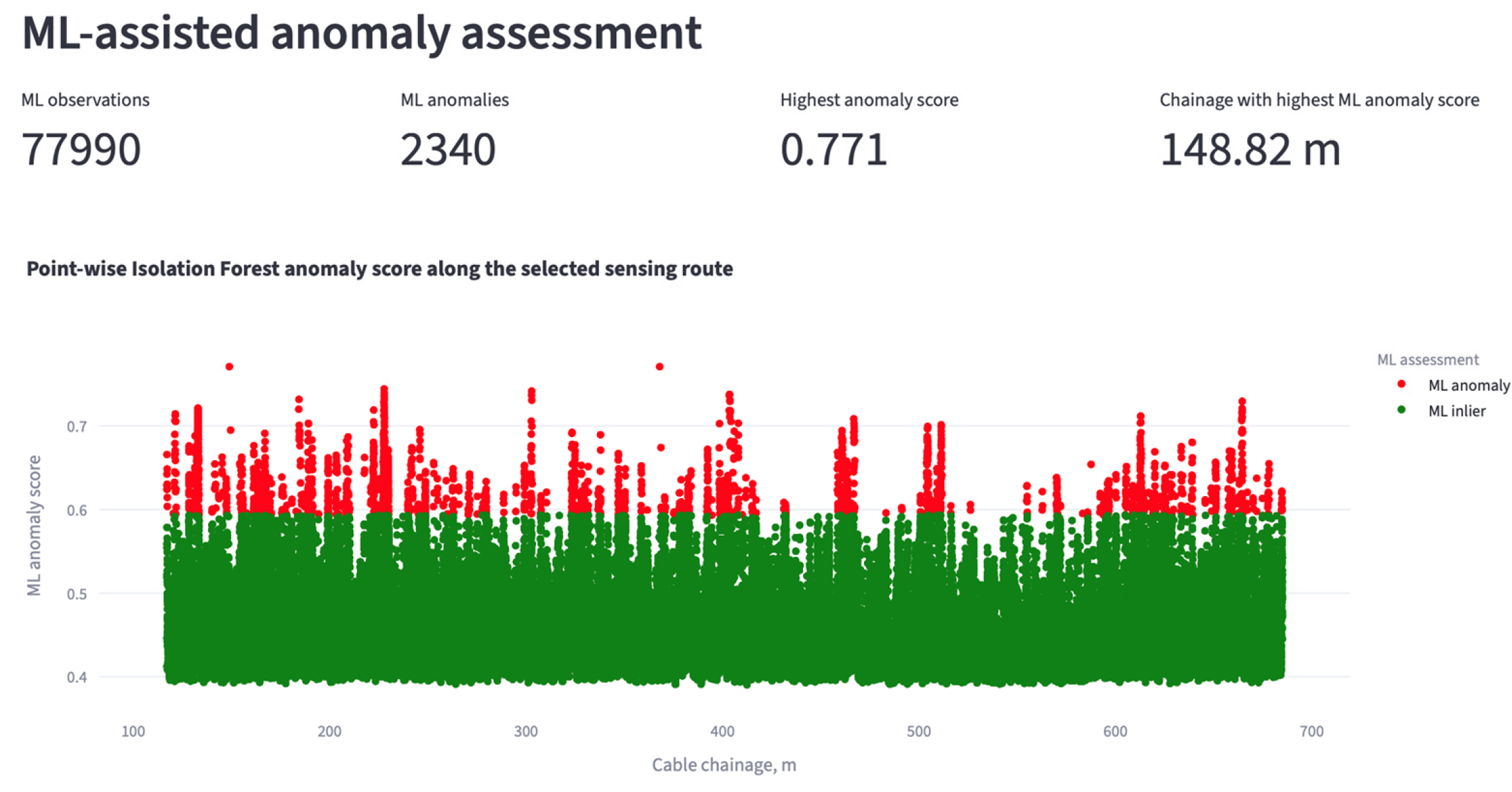
Table 8.
Sensitivity of Isolation Forest screening to the contamination parameter.
Table 9.
Random-seed sensitivity of the highest-ranked Isolation Forest observations.
The pointwise Isolation Forest assessment therefore identified statistically atypical observations while preserving their original spatial correspondence with the DFOS sensing route. The two co-highest-ranked observations demonstrate the value of retaining structural-zone proximity outside the ML representation. Isolation Forest assigned the same maximum anomaly score to observations at 148.82 m and 367.94 m based solely on their response-related variables. Independent structural post-processing subsequently distinguished their route-based context: the first lay within the configured R-Y-Z01 screening neighborhood, whereas the second lay outside the corresponding neighborhood of R-Y-Z03. This comparison shows that structural context provides additional engineering information without influencing the ML anomaly score itself.
Accordingly, the observation at 148.82 m should be treated as a location requiring further engineering assessment because statistical atypicality and route-based structural context coincide there. This correspondence does not constitute evidence of structural deterioration, and its significance must be evaluated together with temporal behavior, strain magnitude, temperature conditions, structural documentation, and independent engineering evidence.
The subsequent Section 3.6 integrates these independent outputs within the interactive visualization environment and examines how the processed DFOS response, structural context, deterministic screening, and ML anomaly assessment can be reviewed jointly for engineering interpretation.
3.6. Interactive Visualization and Integrated Engineering Interpretation
The final stage of the case study consisted of reviewing the processed DFOS results within the integrated Streamlit-based visualization environment described in Section 2.8. The purpose of this stage was not to introduce an additional automated response class but to demonstrate how the mechanical, temporal, thermal, structural, deterministic, and machine learning outputs generated in Section 3.1, Section 3.2, Section 3.3, Section 3.4 and Section 3.5 can be examined together while preserving direct traceability to the original sensing observations.
The application retains the pointwise analytical structure throughout visualization. Each displayed observation remains associated with its sensing-route chainage and acquisition time together with the corresponding analysis strain, reference-relative strain change, temperature information, structural-zone mapping, deterministic screening result, and machine learning output. This common data structure allows the user to move between different analytical views without reconstructing the sensing position from separate files or independently generated plots.
For the Block R Y-direction case study, the interface provides one-dimensional profiles of the processed strain response along the chainage range 117–685 m. The sequential profiles can be compared directly, while mapped structural-response zones are displayed on the same chainage coordinate. This enables localized strain features to be interpreted relative to the six structural-response-zone locations used in the present implementation.
The deterministic screening output is visualized independently from the machine learning results. Observations are shown according to the configured Normal, Warning, and Critical strain-response categories, while the mapped structural zones remain visible as separate spatial references. In the analyzed Block R Y-direction dataset, Warning-level observations were present at selected locations, whereas no observation reached the configured Critical threshold. Consequently, no Critical-plus-structural-proximity condition was identified.
The machine learning view provides a complementary representation of the same monitoring subset. ML inliers and ML anomalies are displayed independently from the deterministic engineering categories, while the continuous anomaly score is retained as a separate variable. This allows statistically atypical observations to be reviewed without implying that they correspond to the deterministic Warning or Critical response levels.
In the principal random_state = 42 analysis reported in Section 3.5, the maximum ML anomaly score was shared by observations at chainages 148.82 m and 367.94 m. Because structural attributes were retained independently of the ML feature matrix, the two observations could subsequently be compared with the mapped response zones. The 148.82 m observation had a chainage offset of 1.18 m from R-Y-Z01 and fell within its configured 2.0 m screening neighborhood, whereas the 367.94 m observation had a chainage offset of 12.94 m from R-Y-Z03 and therefore lay outside the corresponding screening neighborhood.
This association was established only after the ML prediction and anomaly score had been generated. The Isolation Forest model had no information concerning zone identity, zone proximity, screening radius, deterministic response category, or structural-adjacency status. The agreement between the highest-ranked ML chainage and the R-Y-Z01 neighborhood therefore represents an independent engineering context.
Despite this spatial agreement, the observation should not be classified automatically as damaged. The deterministic analysis identified no Critical responses, and the ML score expresses relative statistical atypicality rather than physical damage severity. Further interpretation should consider the corresponding analysis strain, reference-relative change, temperature condition, neighboring observations, temporal persistence, structural documentation, and independent inspection evidence.
This example demonstrates the principal role of the integrated visualization framework. The ML result alone indicates statistical atypicality, while the structural mapping provides information on the location of that observation relative to the mapped foundation response zones. The deterministic screening further shows that the same analyzed dataset did not contain a Critical strain response. These three outputs can therefore be examined jointly without being merged into a single numerical damage index or response class.
In practical engineering use, an ML anomaly should be treated as the starting point for a structured review rather than as a final diagnosis. First, its temporal behavior should be examined to determine whether the response is persistent or isolated. The corresponding analysis strain, reference-relative strain change, and temperature variation should then be reviewed together with the deterministic screening category. Structural-zone proximity should subsequently be checked as an independent contextual factor. If several indicators consistently suggest an unusual local response, the location should be prioritized for further engineering assessment, including comparison with structural documentation, targeted inspection, complementary instrumentation, or structural analysis where warranted.
The integrated interface also preserves the reference-profile information generated in Section 3.2. For a selected sensing observation, the user can examine not only the current analysis strain but also its change relative to the first selected monitoring profile. This enables the response characteristics associated with statistical atypicality—current strain magnitude, reference-relative change, and temperature variation—to be reviewed first, after which the observation can be compared independently with structural proximity and deterministic screening information.
Temperature information is retained in the same analytical workflow. For the present Block R Y-direction dataset, valid temperature matching was available for all 77,990 observations, and the displayed analysis strain therefore corresponded to the temperature-compensated strain throughout the selected analytical subset. The raw strain and temperature-related variables remain available for diagnostic comparison, allowing the user to determine whether a local response changes substantially after thermal correction.
The visualization therefore does not replace the numerical processing described in Section 2.3, Section 2.4, Section 2.5, Section 2.6 and Section 2.7. Instead, it provides a common interface through which the outputs of those procedures can be inspected at their original sensing locations. This is particularly important for localized DFOS response because the engineering interpretation of an observation depends on the coincidence of several independent variables rather than on a single plotted quantity.
In addition to the one-dimensional chainage-based views, the application provides a graphical Plan View for approximate spatial interpretation of the monitored response. The Plan View maps sensing observations onto a predefined representation of the foundation and DFOS route so that locations identified during one-dimensional review can be examined in relation to the broader structural layout.
The Plan View should be interpreted as a visualization aid rather than as a geometrically verified structural model. The displayed positions are not used to calculate the structural-zone proximity ds, which remains defined exclusively from one-dimensional sensing-route chainage. Consequently, the graphical representation does not replace verified CAD/BIM or as-built geometry and should not be used for quantitative distance assessment.
The application also distinguishes between full-resolution analytical processing and graphical rendering. The complete pointwise dataset is retained for temperature compensation, reference-profile comparison, structural mapping, deterministic screening, feature construction, and Isolation Forest analysis. Graphical reduction may be applied only after these calculations have been completed in order to maintain interactive performance.
This distinction is relevant to the present Block R dataset because the analytical subset contains 77,990 pointwise observations. The visualization layer may therefore display a reduced number of points without altering the underlying analytical results. Observations already identified as relevant by deterministic screening, structural adjacency, thermal reclassification, or ML anomaly detection can be retained preferentially in the graphical representation.
The integrated visualization also preserves direct traceability between an observation selected in the interface and the corresponding numerical record. A sensing point identified for further review can therefore be traced to its chainage, acquisition time, analysis strain, reference-relative strain change, temperature condition, nearest mapped structural-response zone, structural proximity, deterministic response category, and ML anomaly output.
This traceability represents an important practical advantage of the developed framework. In conventional spreadsheet-based processing, the engineer may need to compare several separate files and plots to determine whether an unusual sensing value coincides with a structural feature or a particular monitoring time. In the present application, the same information is retained within a common pointwise analytical record and can be reviewed through linked graphical and tabular views. The integrated visualization results are summarized in Figure 9.
Figure 9.
Integrated visualization of the Block R Y-direction DFOS monitoring results within the developed Streamlit application: (a) analysis-strain distribution with deterministic engineering-screening categories and mapped structural-response-zone locations; (b) pointwise Isolation Forest anomaly assessment, including ML inliers, ML anomalies, and the continuous anomaly score along the sensing-route chainage; (c) statistical and temperature-processing summary for the full-resolution analytical dataset; and (d) graphical Plan View for approximate spatial interpretation of the selected sensing-route section and mapped structural-response zones. The analytical calculations were performed using the complete pointwise dataset, whereas graphical rendering may use a reduced number of observations for interactive performance. The Plan View is used as an engineering visualization aid and does not represent a geometrically verified CAD/BIM mapping.
The integrated interpretation demonstrated in the application therefore remains evidence-based rather than automatically diagnostic. A sensing observation becomes more relevant for engineering review when several independent outputs coincide, for example when statistical atypicality occurs together with an elevated or changing strain response and proximity to a mapped structural zone. However, the software does not convert such coincidence into a predefined crack, damage, or failure class.
For the present case study, this distinction is illustrated particularly clearly by the two observations sharing the maximum ML anomaly score. Although both were equally atypical according to Isolation Forest, only the observation at 148.82 m fell within the configured chainage-based screening neighborhood of a mapped structural-response zone. The interface therefore supports prioritization of this location for further review without assigning an unsupported structural damage diagnosis.
The results of Section 3.1, Section 3.2, Section 3.3, Section 3.4, Section 3.5 and Section 3.6 demonstrate that the developed framework can preserve the original pointwise DFOS measurements while integrating temperature compensation, temporal comparison, structural context, deterministic screening, unsupervised anomaly detection, and interactive visualization. The resulting system provides a traceable environment for engineering review of high-density foundation-monitoring data and forms the basis for the broader interpretation discussed in Section 4.
4. Discussion
The results of the present study demonstrate that the practical value of distributed fiber optic sensing for foundation monitoring depends not only on the density of the acquired measurements but also on the ability to preserve their spatial–temporal resolution while adding the contextual information required for engineering interpretation. The developed framework addresses this requirement by maintaining the original pointwise DFOS observations throughout preprocessing, thermo-mechanical correction, reference-profile comparison, structural mapping, deterministic screening, and machine learning analysis. In contrast to workflows based on spatial averaging or interval-level descriptors, each observation remains linked to its original sensing-route chainage and acquisition time. This is particularly important for piled-raft foundations, where local response may develop over relatively short sensing lengths close to columns, core-related regions, and other concentrated load-transfer zones.
The case application to the Block R Y-direction sensing segment confirmed that the proposed workflow can process a comparatively large monitoring dataset without reducing the original spatial resolution. The analyzed subset contained 77,990 pointwise observations from 11 sequential profiles distributed over the chainage range 117–685 m. This pointwise representation is consistent with one of the main advantages of DFOS reported in previous civil-engineering applications, namely its ability to capture distributed response along extended structural regions rather than at isolated instrumented points [3,4,5,6,7,8]. The present study extends this concept from sensing alone to data interpretation by retaining the distributed coordinate throughout all subsequent analytical stages.
An important result of the case study concerns the influence of temperature processing on the monitored response. Temperature compensation was active for the selected Block R dataset, with a mean measured temperature of 5.52 °C and a maximum absolute temperature change of 9.80 °C relative to the selected reference. The resulting analysis strain ranged from −205.5 to 57.9 µε. The comparison between raw and compensated profiles showed that the effect of the temperature correction varied with chainage rather than appearing as a uniform shift along the sensing route. This observation confirms the importance of treating temperature correction as a pointwise operation rather than applying a single global offset to an entire DFOS profile. Such an approach is consistent with the fundamental temperature sensitivity of Brillouin-based distributed sensing [3,5,9].
At the same time, the temperature-compensation procedure used in the present framework should be interpreted within the limits of the adopted processing model. The coefficient was derived from previously reported sensitivity coefficients and was not obtained from a dedicated calibration of the installed sensing system used in the present analysis. This limitation is particularly relevant because the maximum absolute temperature change in the analyzed dataset reached 9.80 °C. Therefore, for quantitative long-term structural assessment, project-specific calibration of the temperature correction coefficient against the actual sensing cable, interrogator configuration, installation condition, and representative environmental range would be preferable.
The reference-profile comparison provides a second important analytical dimension. Profile 17_0115, recorded at 01:15 on 17 May 2024, was used as the first profile of the selected analytical interval, and the remaining ten profiles were compared pointwise with this state. This enables the framework to distinguish between the current magnitude of the measured response and its change relative to the beginning of the selected monitoring period. Such a distinction is important because a location may exhibit a comparatively high absolute strain while remaining temporally stable, whereas another location may show a smaller absolute strain but a larger relative change.
The use of the first selected profile as the reference also introduces an important interpretive limitation. In the present implementation, the reference profile is not an independently verified installation, zero-load, or permanent commissioning baseline. Consequently, characterizes response evolution only within the selected analytical period. It should not be interpreted as the total deformation accumulated since the installation of the sensing system. For long-term monitoring, the framework would benefit from explicit management of several reference states associated with defined structural stages, such as installation, construction, commissioning, and operation.
A further contribution of the framework is the explicit introduction of structural context into the pointwise DFOS dataset. Six mapped response zones were used for the Block R Y-direction analysis at chainages 150, 250, 355, 420, 510, and 620 m. Rather than requiring repeated manual comparison between strain plots and structural drawings, the software automatically calculates the chainage-based distance between each sensing observation and the nearest mapped structural zone. This provides a direct means of determining whether a local response occurs in the neighborhood of a column-, core-, or other structurally significant load-transfer region.
The importance of this structural correspondence is supported by previous monitoring of the same piled-raft foundation [1]. That study demonstrated that the strain field within the raft is spatially non-uniform and that localized tensile response may occur close to concentrated load-transfer regions. The present framework does not transfer physical damage labels from the earlier study to the current dataset; instead, it uses the previous observations to justify why the spatial relationship between distributed strain response and structural location should be retained during interpretation.
The current structural mapping should therefore be regarded as a route-based analytical approximation. The reported values quantify only differences along the one-dimensional DFOS chainage coordinate and do not establish true spatial distance to physical columns, core walls, or other structural elements. In particular, the 1.18 m offset associated with R-Y-Z01 reflects chainage correspondence rather than independently verified geometric proximity. Likewise, the default 2.0 m screening radius is a configurable software-level neighborhood introduced for prioritization and has not been validated as a positional-accuracy tolerance or structural influence radius. For project-level quantitative interpretation, both the chainage-to-structure mapping and the screening radius should be verified using surveyed cable coordinates, as-built documentation, CAD/BIM geometry, or other independent spatial calibration.
The importance of measurement location and structural context has also been demonstrated in related structural-health-monitoring studies. Mao et al. [17] showed that damage sensitivity can be used to guide strain-sensor placement, with measurements obtained at highly sensitive locations providing more reliable damage-identification results. Xiao et al. [18] demonstrated that structural damage identification can also be performed using partial structural models and stiffness-separation concepts, reducing the need for a complete global model. Although these studies concern steel truss bridges and use different identification methodologies, they support the broader principle that monitoring interpretation depends on both informative measurements and their structural context.
The deterministic screening results illustrate the need to separate software-based prioritization from structural damage criteria. The configured thresholds classify observations as Normal for µε, Warning for µε, and Critical for µε. For the selected Block R Y-direction dataset, the minimum analysis strain of −205.5 µε fell within the Warning range, while no observation reached the Critical threshold. Accordingly, the application reported zero observations satisfying the combined Critical-plus-structural-proximity condition.
This result should not be interpreted as a general statement that no localized foundation response was present. It indicates only that none of the analyzed observations satisfied the particular configured Critical criterion. The thresholds of 100 and 300 µε are software screening parameters introduced to organize monitoring observations and are not presented as universal reinforced-concrete failure limits, validated crack-initiation thresholds, or project-specific structural action levels. Their principal role is to provide a transparent and reproducible deterministic screening layer. Establishment of formal engineering action thresholds would require calibration against structural design criteria, long-term DFOS records, independent inspection evidence, and, where appropriate, numerical structural analysis.
Although the framework was demonstrated using a piled-raft foundation, the proposed workflow can also be applied to other foundation systems instrumented with DFOS. However, the strain-response ranges used for deterministic Normal, Warning, and Critical screening should be adapted to the specific foundation type, structural system, material properties, loading conditions, and monitoring configuration. Therefore, the threshold values adopted in the present study should not be transferred directly to other foundation systems without project-specific engineering justification.
The machine learning analysis provided a complementary response-based perspective. Isolation Forest was fitted to 77,990 observations using analysis strain, reference-relative strain change, and temperature change. Structural-zone proximity was deliberately excluded from model fitting and scoring. With contamination set to 0.03, the model identified 2340 ML anomalies. Two observations, at chainages 148.82 m and 367.94 m, shared the maximum displayed anomaly score of 0.770908.
Excluding structural-zone proximity from the ML vector preserves the independence of subsequent structural interpretation. If proximity was used both as a model input and as evidence during interpretation, correspondence between an anomaly and a mapped zone would be partly embedded in the feature design. In the adopted workflow, Isolation Forest evaluates only mechanical, temporal, and thermal response variables. Structural-zone identity and proximity are introduced only after ML inference as an independent engineering-context layer.
Independent post-processing distinguished the structural context of the two co-highest-ranked observations. The observation at 148.82 m had a chainage offset of 1.18 m from R-Y-Z01 and fell within its configured 2.0 m screening neighborhood, whereas the observation at 367.94 m had a 12.94 m chainage offset from R-Y-Z03 and lay outside the corresponding neighborhood. Because structural-zone proximity was excluded from the feature vector, this difference in structural context was not embedded in the Isolation Forest scores and emerged only during independent post-processing.
This result is methodologically informative but does not establish structural damage. The model was not trained using labeled damaged and undamaged states, and deterministic screening identified no Critical observations. The response at 148.82 m should therefore be treated as a statistically atypical observation located within an independently mapped structural neighborhood. Its physical significance requires a review of strain magnitude, reference-relative evolution, temperature condition, temporal persistence, structural documentation, and independent engineering evidence.
The spatial coincidence between the independently detected ML anomaly and R-Y-Z01 is therefore interpreted as a useful engineering-screening result rather than as independent verification of damage. It demonstrates the value of combining response-based anomaly detection with separately retained structural context, while the physical condition of the foundation can only be established through additional engineering assessment and independent evidence.
This distinction between statistical anomaly and physical damage is particularly important in structural health monitoring, where labeled field damage data are frequently unavailable [10,11,12,13,19]. Under such conditions, unsupervised learning can provide a useful means of reducing the volume of measurements requiring immediate inspection, but it cannot by itself establish the underlying structural mechanism. The role of Isolation Forest in the present study is therefore screening and prioritization rather than diagnosis.
The contamination parameter should be regarded as a binary screening setting rather than as a calibrated structural parameter. The sensitivity analysis performed at contamination values of 0.01, 0.03, and 0.05 confirmed that the size of the binary anomaly subset depends directly on the selected decision threshold: 780, 2340, and 3900 observations were classified as ML anomalies, respectively. Consequently, the number of binary anomaly labels should not itself be interpreted as evidence of structural abnormality or as an independent measure of screening performance.
More importantly, the relative anomaly-score ranking remained stable across the tested settings. The observations at chainages 148.82 m and 367.94 m retained the joint maximum anomaly score of 0.770908 and remained within the binary anomaly subset even under the most restrictive tested setting of contamination = 0.01. This indicates that their high screening priority is not attributable solely to the principal 3% decision threshold. Observations closer to the binary classification boundary are more sensitive to the selected contamination value and should consequently be interpreted with greater caution.
The sensitivity analysis does not establish an optimal contamination value. Because independently labeled damaged and undamaged observations are unavailable, none of the tested values can presently be validated as a structure-specific decision threshold. The value of 0.03 is therefore retained as the principal exploratory screening configuration, while the 0.01 and 0.05 analyses are used to assess the robustness of the highest-priority observations to the selected binary cutoff.
The random-seed sensitivity assessment further showed that the exact numerical Isolation Forest score is stochastic and should not be treated as a fixed physical quantity. The principal value of 0.770908 corresponds specifically to random_state = 42. Across the 11 tested random states, the observations at 148.82 m and 367.94 m remained classified as ML anomalies in every run and were jointly highest ranked in 10 runs. In one realization, random_state = 6, an observation at 132.82 m received a marginally higher score, while the 148.82 m and 367.94 m observations remained jointly second highest. The results therefore support strong but not absolute stochastic stability of the principal high-priority locations. This reinforces the need to interpret the ML output through ranking patterns and an independent engineering context rather than through a single anomaly-score value from one stochastic realization.
The pointwise nature of the machine learning procedure is another relevant aspect of the proposed framework. No spatial interval aggregation was applied before Isolation Forest fitting. Consequently, local observations remain visible within the anomaly-score distribution rather than being smoothed by neighboring measurements. This is advantageous where local response is expected over relatively short portions of the cable. At the same time, pointwise analysis increases the sensitivity to isolated measurement fluctuations. Individual ML anomalies should therefore be interpreted with particular caution when they are not accompanied by repeatable temporal behavior or meaningful structural context.
An additional consideration in machine-learning-based monitoring is the complexity of the input representation. Feature-selection studies have shown the importance of limiting irrelevant or redundant information when working with high-dimensional datasets [20]. In an image-based convolutional neural network application, Kabir and Garg [21] further discussed input-data complexity in relation to Kolmogorov complexity and demonstrated that conversion of natural images to simpler binarized representations reduced computational demand and improved model convergence, stability, and predictive performance. Although these studies address image-based learning problems that differ substantially from the present pointwise DFOS application, the underlying principle supports the use of compact and physically interpretable input representations. In the present framework, the Isolation Forest input is deliberately restricted to three response-related variables—analysis strain, reference-relative strain change, and temperature change—while structural, deterministic, and visualization variables are retained outside the ML feature space. However, no formal Kolmogorov-complexity metric or feature-selection optimization was applied in the present study, and the absence of independently labeled damage states prevents the attribution of a quantitative accuracy improvement to reduced input complexity. Future work could therefore examine whether alternative compact feature representations or formal complexity-control approaches improve computational efficiency and robustness while preserving physically meaningful DFOS information.
For this reason, the present framework intentionally retains the deterministic, structural, thermal, temporal, and ML outputs as independent quantities rather than combining them into a weighted response index. No numerical weights are assigned to strain magnitude, , temperature variation, structural proximity, or anomaly score. This avoids introducing an arbitrary composite indicator whose physical meaning would be difficult to validate. Instead, engineering attention increases when several independent observations support the same sensing location. Accordingly, the framework is intended to support a staged engineering review in which ML-based statistical screening is followed by an examination of temporal persistence, strain magnitude, thermal influence, deterministic screening, structural context, and, where justified, independent inspection or structural analysis.
The developed visualization environment is also important to this interpretation. The one-dimensional profiles, structural-zone markers, deterministic response categories, temperature information, reference-relative variables, and ML anomaly scores remain linked through a common pointwise dataset. This allows a statistically atypical observation to be traced directly to its original chainage and acquisition time and then examined together with the corresponding mechanical and environmental quantities. Such traceability is a practical advantage over workflows in which strain, temperature, structural location, and anomaly results are analyzed in separate files or plots.
The graphical Plan View extends this traceability by providing an approximate two-dimensional representation of the sensing results relative to the foundation layout. However, its role remains qualitative. The current implementation does not reconstruct the exact installed cable geometry from verified CAD/BIM coordinates, and the Plan View is not used to calculate structural proximity. It should therefore be considered an engineering visualization aid rather than a geometrically validated digital model.
Although the present case study was demonstrated on a reinforced-concrete piled-raft foundation, the overall analytical workflow is not intrinsically restricted to this foundation type. The same sequence of pointwise DFOS preprocessing, temperature compensation, reference-profile comparison, response-based anomaly detection, deterministic screening, and post-ML structural interpretation could be applied to other instrumented foundation systems, provided that strain and, where required, temperature measurements can be expressed within a consistent sensing-route coordinate system. Potential applications may include raft foundations, strip or combined footings, pile caps, and other foundation systems instrumented with distributed sensing.
Several limitations of the present case study should be acknowledged. First, the reported analysis is based on 11 sequential profiles collected over a relatively short monitoring interval and on a single Block R Y-direction sensing segment. The results demonstrate the operation of the complete analytical framework but do not constitute long-term validation of the anomaly patterns or structural response. Longer monitoring periods are required to determine whether the identified features persist under different construction, commissioning, seasonal, and operational conditions. Reference-state selection represents an additional source of analytical sensitivity because is included in the Isolation Forest feature vector. Different reference profiles may lead to different values and, consequently, to changes in anomaly ranking. Future long-term implementations should therefore evaluate reference-selection sensitivity and consider the use of physically defined reference states associated with installation, commissioning, or representative operational conditions.
Second, independent validation of the ML anomalies is not available for every pointwise observation. The current dataset does not include labels identifying confirmed cracking, excessive deformation, or other physical mechanisms. Consequently, model performance cannot presently be expressed through conventional supervised-classification metrics such as accuracy, precision, recall, or F1-score. Future validation should therefore compare the ML outputs with visual inspection, conventional instrumentation, structural analysis, and documented construction events.
Third, the current structural mapping should be replaced by verified installation-based mapping for project-level deployment. Integration of as-built DFOS chainage information with structural drawings or BIM coordinates would allow the present one-dimensional proximity measure to be supplemented by geometrically meaningful two-dimensional or three-dimensional spatial relationships.
Fourth, the workflow remains file-based. Data are imported from Excel workbooks rather than streamed directly from the optical interrogator. This configuration is suitable for research analysis, commissioning review, and periodic monitoring, but a fully operational real-time system would require automated interrogator connectivity, structured database storage, continuous data-quality control, event handling, and automated updating of analytical outputs.
Future development should therefore focus on validation against independent engineering evidence, longer-term reference-state management, evaluation of model stability over extended monitoring periods, temporal tracking of repeated anomalies, broader validation of the Isolation Forest configuration, verification of structural mapping using CAD/BIM or as-built information, direct connection to monitoring databases, and comparison of identified anomalies with independent structural observations. Integration with BIM- and digital-twin-based environments would provide a natural extension because the present framework already organizes the sensing data according to spatial, temporal, structural, and analytical attributes [22,23,24].
Overall, the results indicate that the main benefit of the proposed approach lies in combining high-density DFOS data with interpretable structural and statistical context while preserving the original sensing resolution. The framework does not replace structural engineering judgement and does not convert ML output directly into damage labels. Instead, it reduces the volume of distributed monitoring information requiring manual examination and provides a traceable basis for identifying locations where mechanical response, temporal evolution, thermal conditions, structural proximity, and statistical atypicality warrant further investigation.
5. Conclusions
Based on the developed analytical framework and its application to the Block R Y-direction segment of the piled-raft foundation, the following conclusions can be drawn:
- An interactive machine-learning-assisted DFOS framework was developed for building foundation monitoring. The framework integrates numerical preprocessing, strain–temperature matching and compensation, reference-profile comparison, structural mapping, deterministic engineering screening, pointwise multivariate analysis, Isolation Forest anomaly detection, and interactive visualization. The principal methodological feature is the preservation of the original pointwise spatial and temporal coordinates throughout the complete analytical workflow.
- The framework was demonstrated using 11 sequential DFOS monitoring profiles recorded on 17 May 2024 between 01:15 and 02:55. The analyzed Block R Y-direction segment covered chainages of 117–685 m and comprised 77,990 pointwise observations, corresponding to 7090 observations per profile. Valid temperature matching was obtained for all observations. The mean temperature was 5.52 °C, and the maximum absolute temperature change relative to the selected reference reached 9.80 °C. Following thermo-mechanical processing, the analysis strain ranged from −205.5 to 57.9 µε. The spatial variation between raw and compensated strain confirmed that temperature correction should be applied pointwise rather than as a uniform adjustment over the complete DFOS profile.
- Reference-profile comparison and structural mapping provided temporal and structural context for each sensing observation. Profile 17_0115 was used as the analytical reference for evaluating short-term strain evolution and should be interpreted as a period-specific reference rather than an installation, zero-load, or permanent commissioning baseline. Six structural-response zones were mapped at chainages 150, 250, 355, 420, 510, and 620 m. The calculated proximity represents a one-dimensional chainage-based distance to the nearest mapped structural zone and not a two-dimensional Euclidean distance to a physical column or core element.
- Deterministic engineering screening identified Warning-level responses but no Critical observations. The minimum analysis strain of −205.5 µε remained within the Warning range, while no observation reached the configured Critical threshold of |ε| ≥ 300 µε. Consequently, none of the 77,990 observations satisfied the combined Critical-plus-structural-proximity condition. The adopted thresholds should be interpreted as configurable software screening parameters rather than universal reinforced-concrete failure or crack-initiation criteria.
- Isolation Forest provided an independent statistical screening layer complementary to deterministic strain-based assessment. The model used three response-related input variables: analysis strain, reference-relative strain change, and temperature change. Structural-zone proximity was excluded from fitting and scoring and retained only for post-ML engineering interpretation. With contamination set to 0.03, the model identified 2340 ML anomalies. Sensitivity analysis using contamination values of 0.01, 0.03, and 0.05 produced 780, 2340, and 3900 binary ML anomalies, respectively, confirming that the size of the flagged subset depends on the selected binary decision threshold. However, the observations at chainages 148.82 m and 367.94 m retained the joint maximum anomaly score of 0.770908 and remained classified as ML anomalies under all three settings. Their screening priority was therefore stable within the tested contamination range, although this stability should not be interpreted as validation of structural damage. Random-seed analysis using random states 0–9 and 42 further showed that the exact anomaly-score magnitude varied between model realizations. Nevertheless, the observations at 148.82 m and 367.94 m remained ML anomalies in all 11 runs and were jointly highest ranked in 10 of them. Thus, the principal high-priority locations showed strong, although not absolute, stochastic stability, while the specific maximum score of 0.770908 should be associated with the principal random_state = 42 realization. Independent post-processing showed that the first had a 1.18 m chainage offset from R-Y-Z01 and fell within its configured 2.0 m route-based screening neighborhood, whereas the second had a 12.94 m chainage offset from R-Y-Z03 and lay outside the corresponding neighborhood. Because structural proximity was not supplied to the model, this difference represents an independent engineering context rather than an effect of ML feature selection. The ML results nevertheless represent statistical atypicality and should not be interpreted directly as evidence of cracking, excessive settlement, or structural damage.
- The framework should be regarded as an engineering decision-support and prioritization tool rather than an autonomous damage detection system. Current limitations include the short monitoring interval, analysis of one route segment, route-based rather than geometrically verified mapping, an adopted temperature-compensation coefficient, and the absence of labeled damage observations. Future work should address longer-term validation, validation of the contamination setting against independent engineering evidence, independent inspection evidence, verified CAD/BIM or as-built mapping, multiple reference states, and direct connection to the monitoring database and optical interrogator.
Supplementary Materials
The following supporting information can be downloaded at https://www.mdpi.com/article/10.3390/buildings16204054/s1: Supplementary File S1 contains the complete Python source code used for numerical preprocessing, temperature compensation, reference-profile comparison, feature construction, Isolation Forest analysis, contamination-sensitivity assessment, random-seed sensitivity analysis, and visualization of the presented case study.
Author Contributions
Conceptualization, A.B. and B.P.T.; software, A.B. and I.Z.; formal analysis, A.S. and L.D.G.; investigation, I.Z. and B.P.T.; resources, A.S. and L.D.G.; writing—original draft, A.B. and B.P.T.; writing—review and editing, A.S.; visualization, I.Z. and B.P.T.; supervision, A.B.; project administration, A.B.; funding acquisition, A.B. All authors have read and agreed to the published version of the manuscript.
Funding
This work was funded by Committee of Science of the Ministry of Science and Higher Education of the Republic of Kazakhstan (Grant No. AP22688230).
Data Availability Statement
The raw data supporting the conclusions of this article will be made available by the authors on request.
Acknowledgments
The authors gratefully acknowledge Smart Sensing Technology Sdn Bhd (Shah Alam, Malaysia) for their technical advice and cooperation, in particular B.P.T. for his assistance related to DFOS installation and signal interpretation. The experimental work was supported by the field engineering team and subcontractors involved in the DFOS cable installation, bonding, and load testing procedures. Their practical expertise and on-site coordination greatly contributed to the successful execution of the test program.
Conflicts of Interest
Author Mr. Bun Pin Tee was employed by the company Smart Sensing Technology Sdn Bhd. The remaining authors declare that the research was conducted in the absence of any commercial or financial relationships that could be construed as a potential conflict of interest.
References
- Buranbayeva, A.; Zhussupbekov, A.; Sarsembayeva, A.; Omarov, A. Evaluation of the Structural Health Monitoring Results of the Applied Fiber Optics in the Pile-Raft Foundations of a High-Rise Building. Appl. Sci. 2022, 12, 11728. [Google Scholar] [CrossRef] [Scilit]
- Buranbayeva, A.; Sarsembayeva, A.; Tee, B.P.; Zhumadilov, I.; Orazbekova, G. Performance Evaluation of Fixed-Point DFOS Cables for Structural Monitoring of Reinforced Concrete Elements. Infrastructures 2025, 10, 349. [Google Scholar] [CrossRef] [Scilit]
- Barrias, A.; Casas, J.R.; Villalba, S. A Review of Distributed Optical Fiber Sensors for Civil Engineering Applications. Sensors 2016, 16, 748. [Google Scholar] [CrossRef] [Scilit]
- Bado, M.F.; Casas, J.R. A Review of Recent Distributed Optical Fiber Sensors Applications for Civil Engineering Structural Health Monitoring. Sensors 2021, 21, 1818. [Google Scholar] [CrossRef] [Scilit]
- Kishida, K.; Imai, M.; Kawabata, J.; Guzik, A. Distributed Optical Fiber Sensors for Monitoring of Civil Engineering Structures. Sensors 2022, 22, 4368. [Google Scholar] [CrossRef] [Scilit]
- Minardo, A.; Zeni, L.; Coscetta, A.; Catalano, E.; Zeni, G.; Damiano, E.; De Cristofaro, M.; Olivares, L. Distributed Optical Fiber Sensor Applications in Geotechnical Monitoring. Sensors 2021, 21, 7514. [Google Scholar] [CrossRef] [Scilit]
- Mohamad, H.; Soga, K.; Pellew, A.; Bennett, P.J. Performance Monitoring of a Secant-Piled Wall Using Distributed Fiber Optic Strain Sensing. J. Geotech. Geoenviron. Eng. 2011, 137, 1236–1243. [Google Scholar] [CrossRef] [Scilit]
- Soga, K.; Luo, L. Distributed Fiber Optics Sensors for Civil Engineering Infrastructure Sensing. J. Struct. Integr. Maint. 2018, 3, 1–21. [Google Scholar] [CrossRef] [Scilit]
- Bao, X.; Chen, L. Recent Progress in Distributed Fiber Optic Sensors. Sensors 2012, 12, 8601–8639. [Google Scholar] [CrossRef] [Scilit]
- Farrar, C.R.; Worden, K. An Introduction to Structural Health Monitoring. Philos. Trans. R. Soc. A Math. Phys. Eng. Sci. 2007, 365, 303–315. [Google Scholar] [CrossRef] [Scilit]
- Figueiredo, E.; Park, G.; Farrar, C.R.; Worden, K.; Figueiras, J. Machine Learning Algorithms for Damage Detection under Operational and Environmental Variability. Struct. Health Monit. 2011, 10, 559–572. [Google Scholar] [CrossRef] [Scilit]
- Salehi, H.; Burgueño, R. Emerging Artificial Intelligence Methods in Structural Engineering. Eng. Struct. 2018, 171, 170–189. [Google Scholar] [CrossRef] [Scilit]
- Eltouny, K.; Gomaa, M.; Liang, X. Unsupervised Learning Methods for Data-Driven Vibration-Based Structural Health Monitoring: A Review. Sensors 2023, 23, 3290. [Google Scholar] [CrossRef] [Scilit]
- Liu, F.T.; Ting, K.M.; Zhou, Z.-H. Isolation Forest. In Proceedings of the 2008 IEEE International Conference on Data Mining, Pisa, Italy, 15–19 December 2008; pp. 413–422. [Google Scholar] [CrossRef] [Scilit]
- Golder Associates (HK) Limited. Distributed Fibre Optic Strain Sensing System for Basement Slab: Detailed Design Submission; Project Technical Report No. 178112027-007R. Astana, Kazakhstan. Unpublished project document, 2019.
- Pedregosa, F.; Varoquaux, G.; Gramfort, A.; Michel, V.; Thirion, B.; Grisel, O.; Blondel, M.; Prettenhofer, P.; Weiss, R.; Dubourg, V.; et al. Scikit-learn: Machine Learning in Python. J. Mach. Learn. Res. 2011, 12, 2825–2830. [Google Scholar]
- Mao, Y.; Xiao, F.; Tian, G.; Xiang, Y. Sensitivity Analysis and Sensor Placement for Damage Identification of Steel Truss Bridge. Structures 2025, 73, 108310. [Google Scholar] [CrossRef] [Scilit]
- Xiao, F.; Mao, Y.; Tian, G.; Chen, G.S. Partial-Model-Based Damage Identification of Long-Span Steel Truss Bridge Based on Stiffness Separation Method. Struct. Control Health Monit. 2024, 2024, 5530300. [Google Scholar] [CrossRef] [Scilit]
- Sony, S.; Laventure, S.; Sadhu, A. A Literature Review of Next-Generation Smart Sensing Technology in Structural Health Monitoring. Struct. Control Health Monit. 2019, 26, e2321. [Google Scholar] [CrossRef] [Scilit]
- Bolon-Canedo, V.; Remeseiro, B. Feature Selection in Image Analysis: A Survey. Artif. Intell. Rev. 2020, 53, 2905–2931. [Google Scholar] [CrossRef] [Scilit]
- Kabir, H.; Garg, N. Machine Learning Enabled Orthogonal Camera Goniometry for Accurate and Robust Contact Angle Measurements. Sci. Rep. 2023, 13, 1497. [Google Scholar] [CrossRef] [Scilit]
- Boje, C.; Guerriero, A.; Kubicki, S.; Rezgui, Y. Towards a Semantic Construction Digital Twin: Directions for Future Research. Autom. Constr. 2020, 114, 103179. [Google Scholar] [CrossRef] [Scilit]
- Torzoni, M.; Tezzele, M.; Mariani, S.; Manzoni, A.; Willcox, K.E. A Digital Twin Framework for Civil Engineering Structures. Comput. Methods Appl. Mech. Eng. 2024, 418, 116584. [Google Scholar] [CrossRef] [Scilit]
- Buranbayeva, A.; Sarsembayeva, A.; Mussakhanova, S.T. Geomonitoring of the foundation of a high-rise building applied fiber optics. In Smart Geotechnics for Smart Societies; CRC Press: Boca Raton, FL, USA, 2023; ISBN 978-1-003-29912-7. [Google Scholar] [CrossRef] [Scilit]
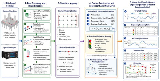
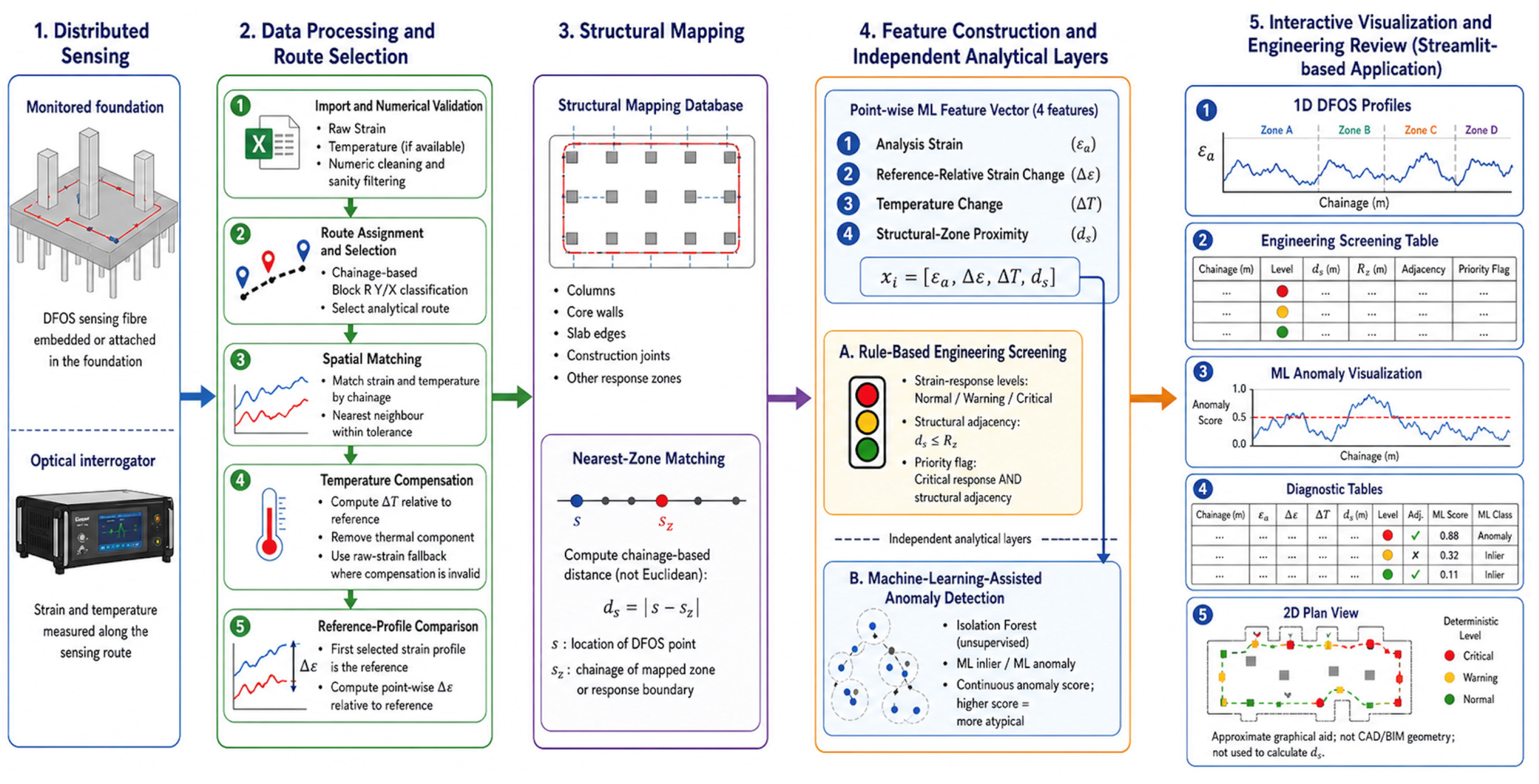
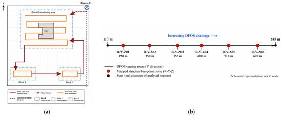
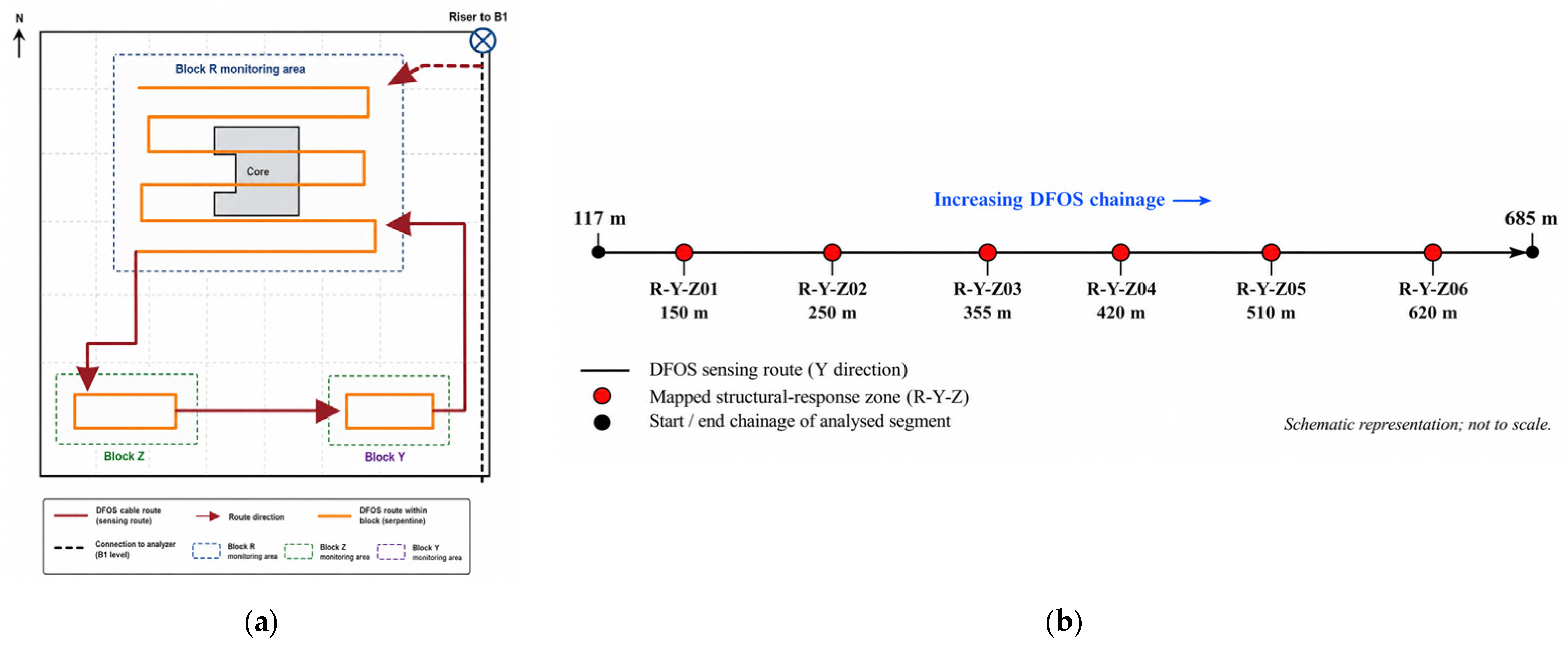
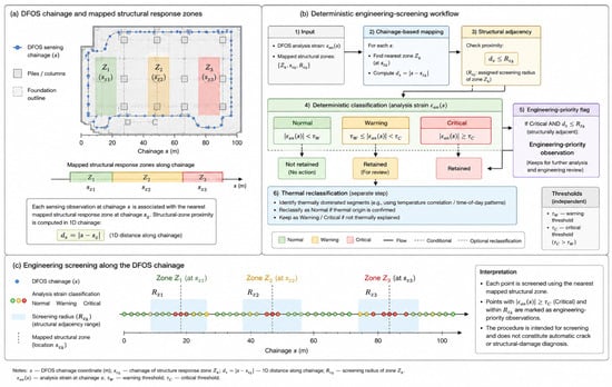
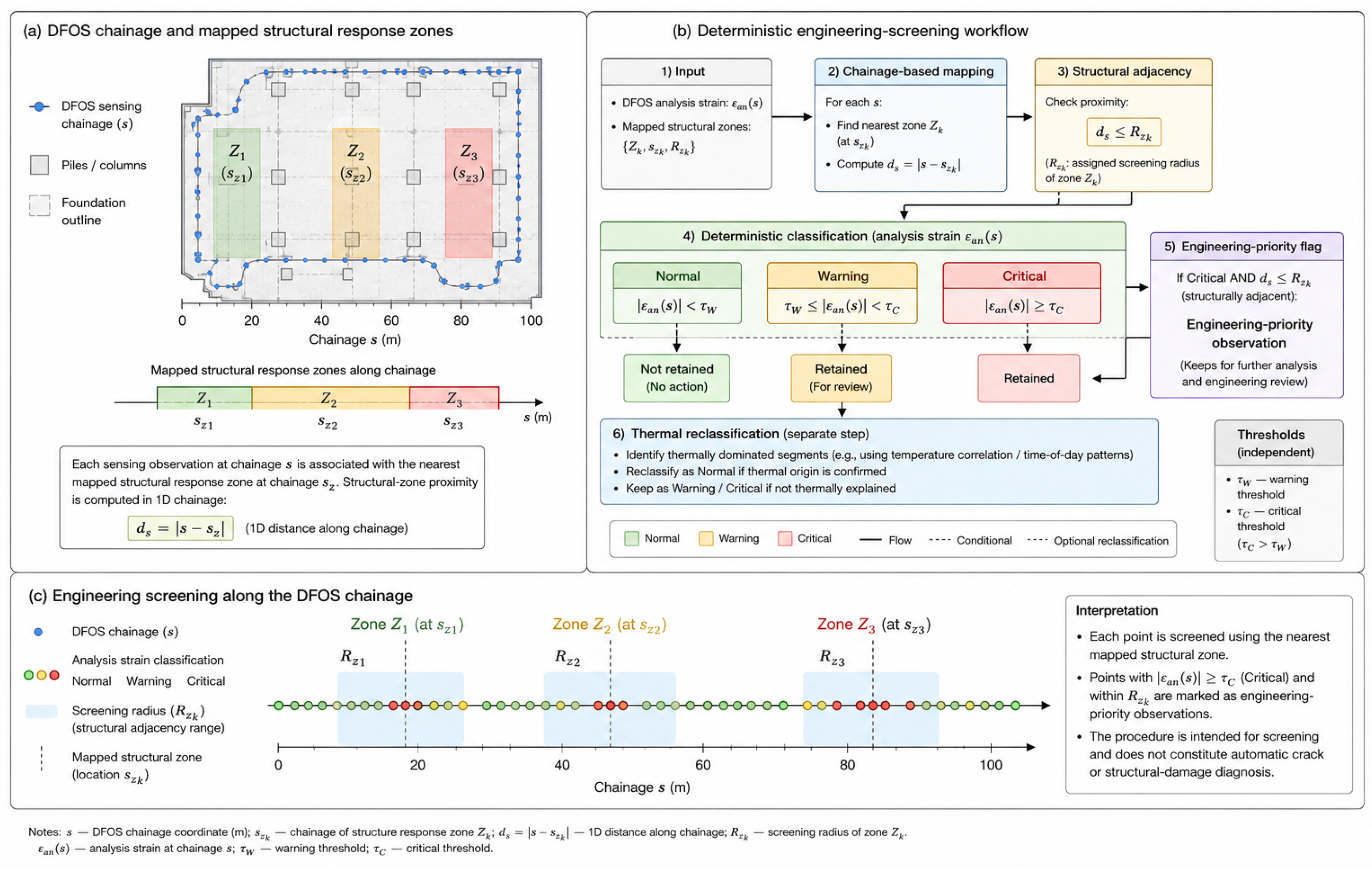
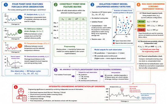
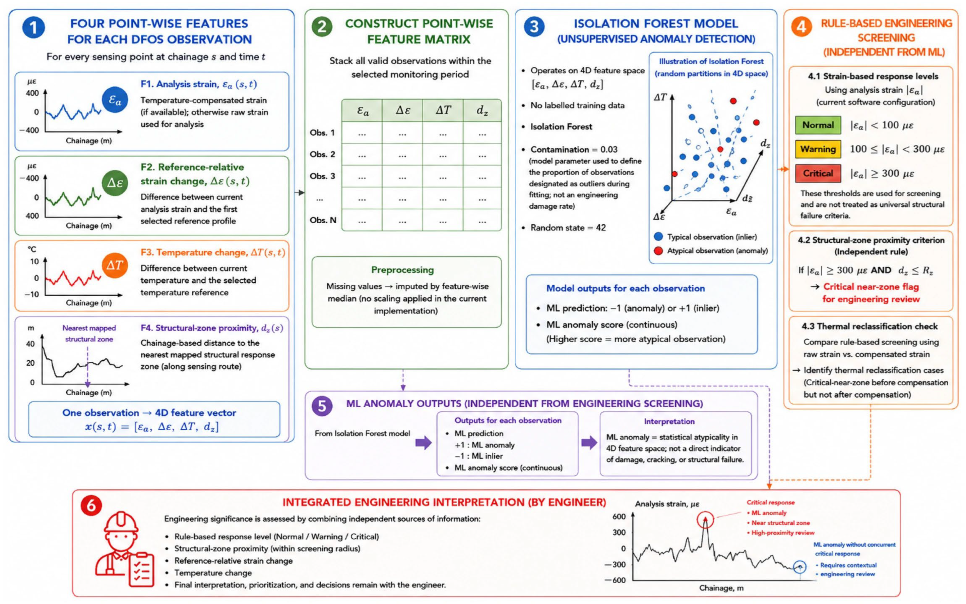
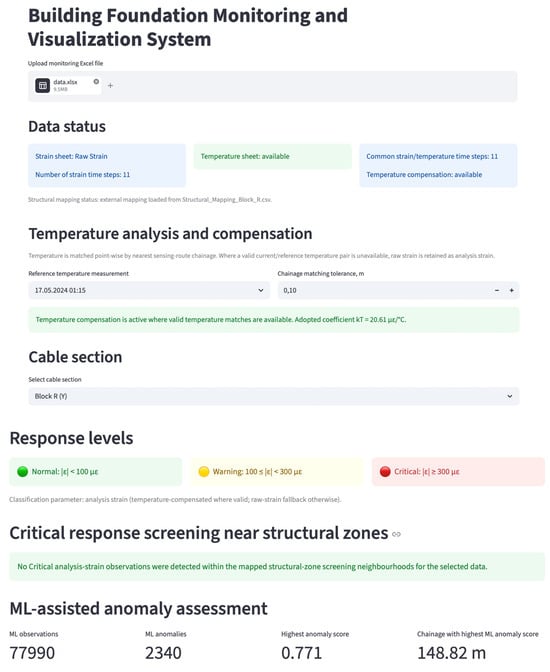
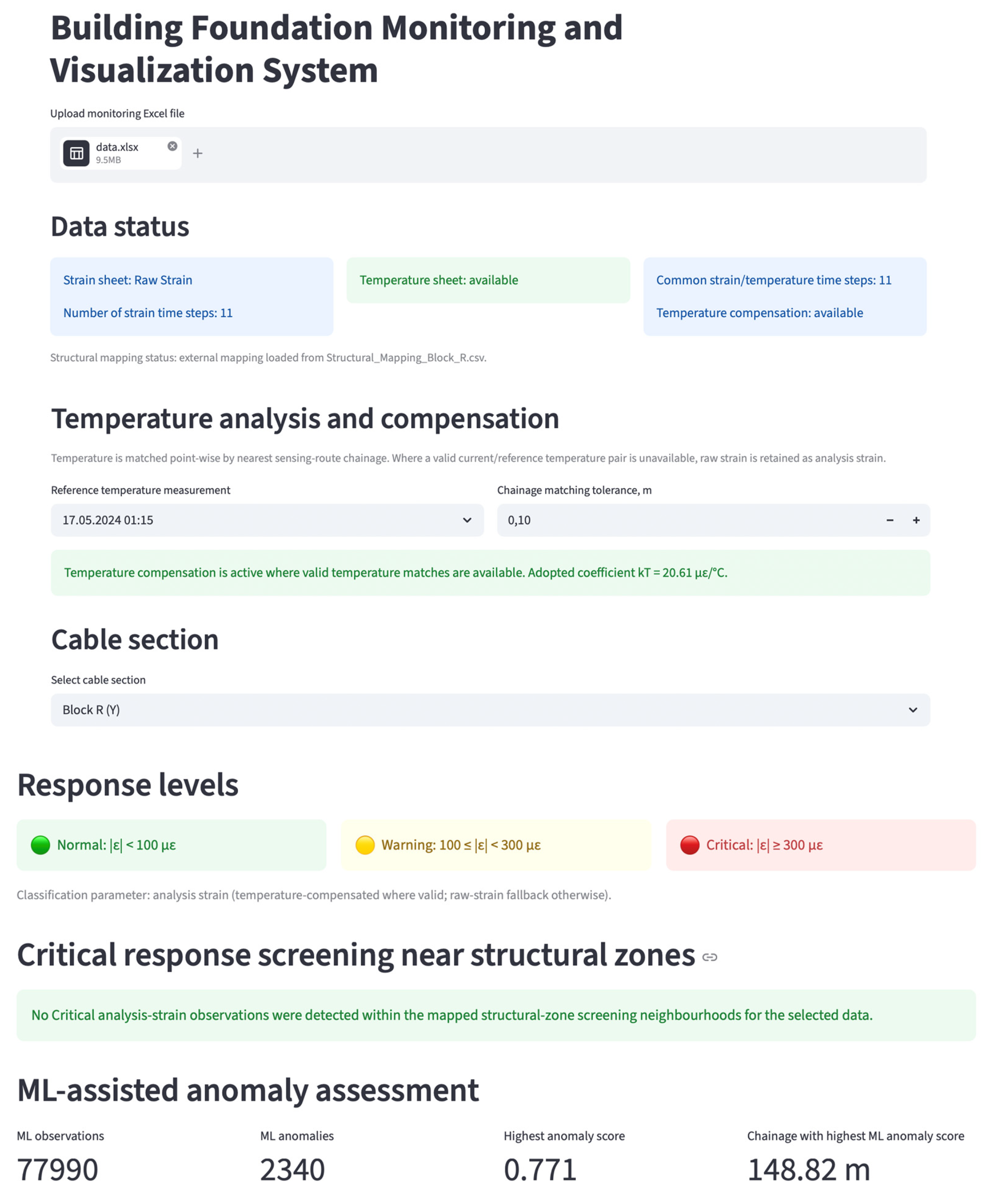
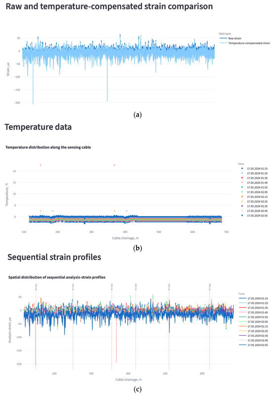
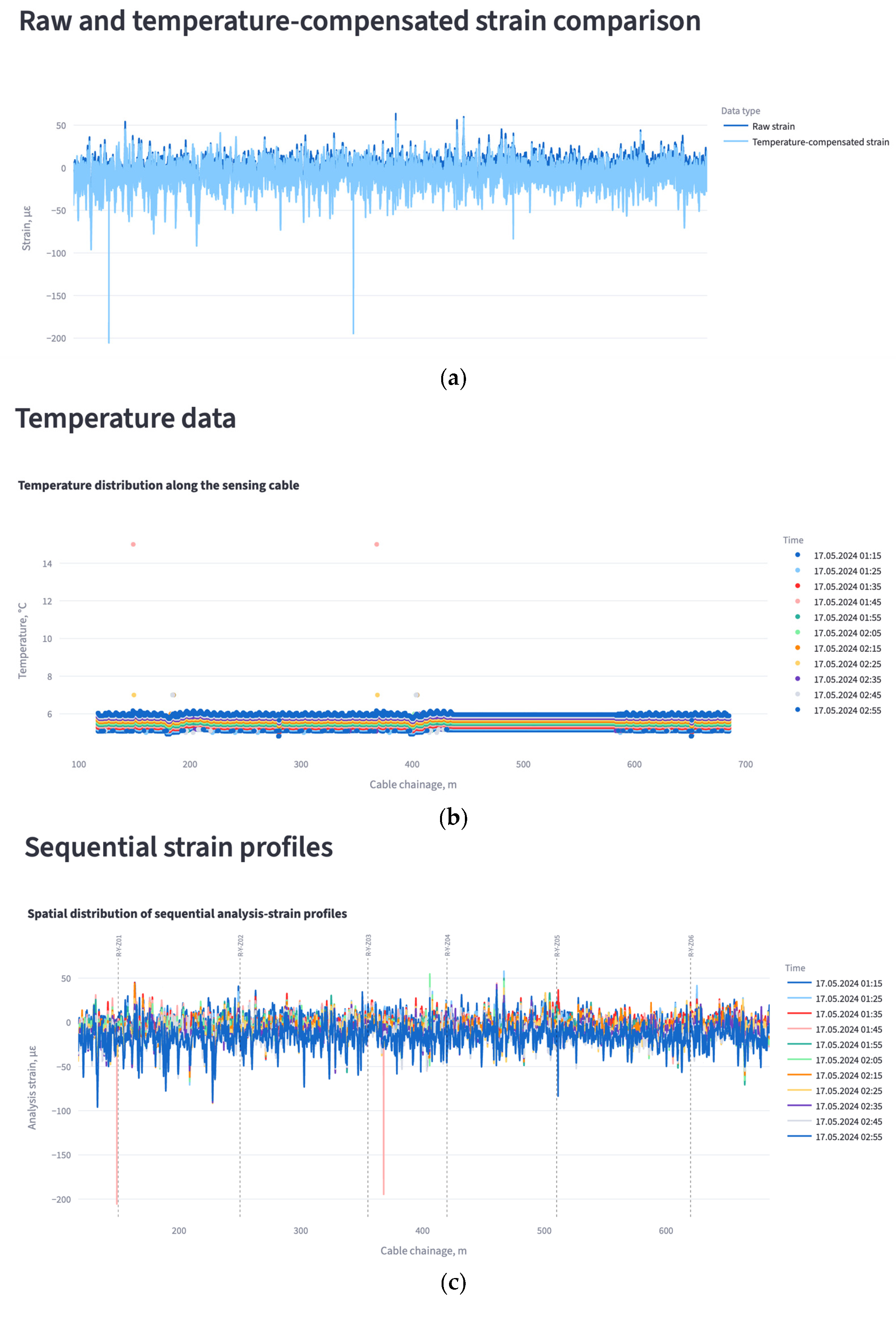
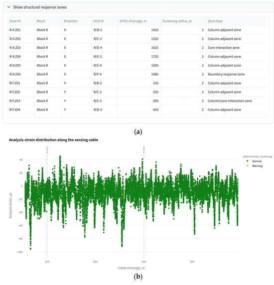
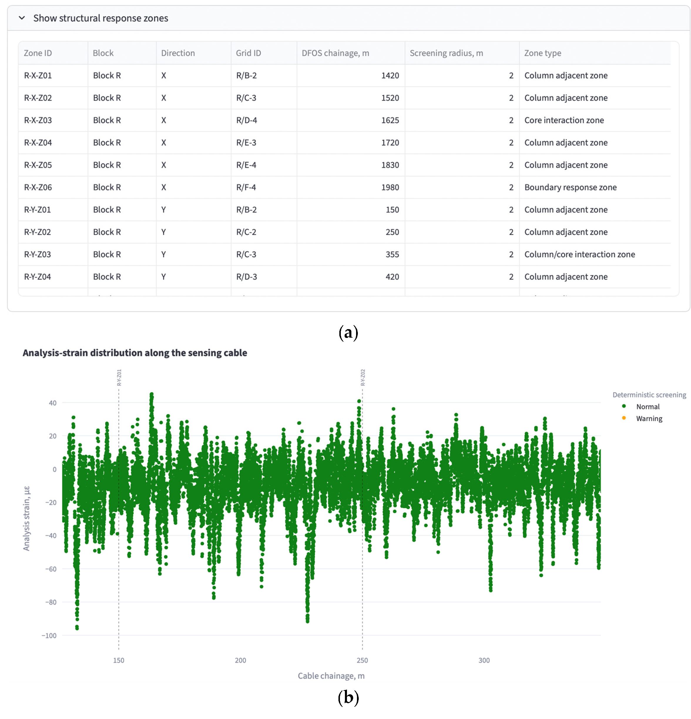
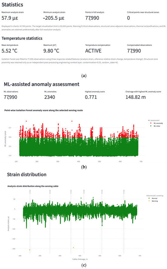
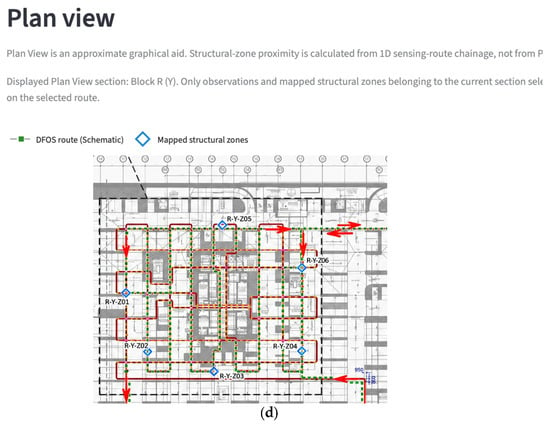
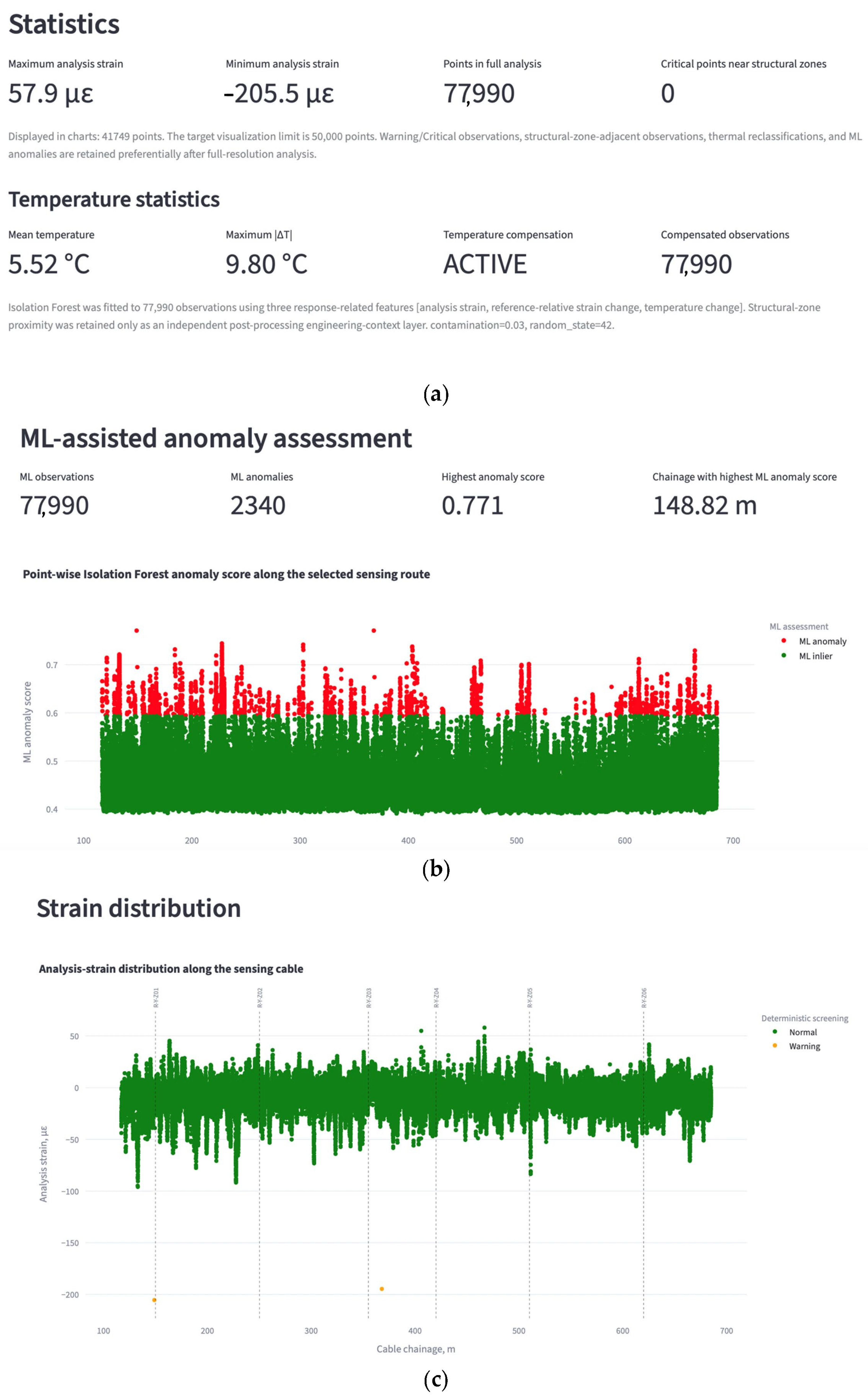
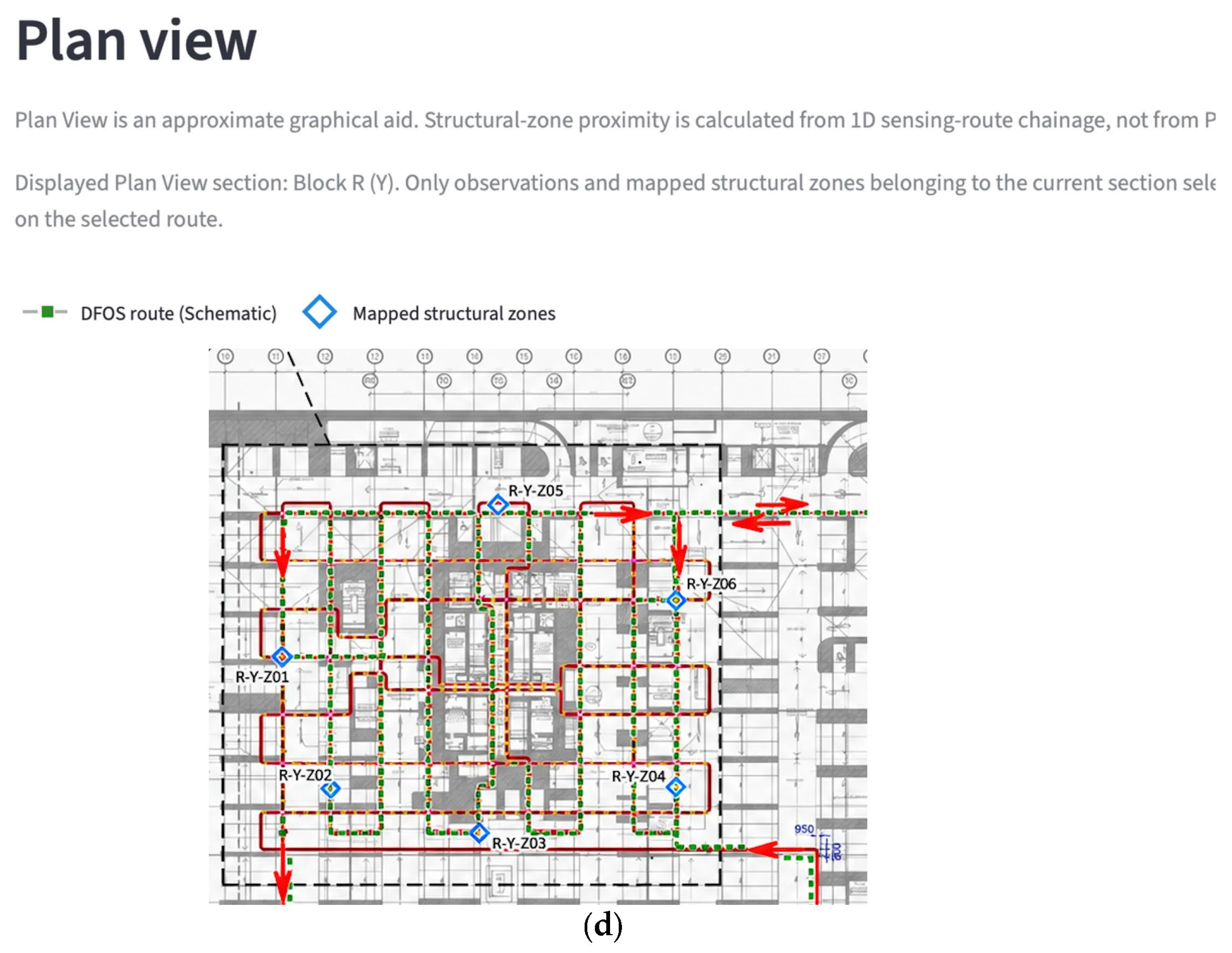

Disclaimer/Publisher’s Note: The statements, opinions and data contained in all publications are solely those of the individual author(s) and contributor(s) and not of MDPI and/or the editor(s). MDPI and/or the editor(s) disclaim responsibility for any injury to people or property resulting from any ideas, methods, instructions or products referred to in the content. |
© 2026 by the authors. Licensee MDPI, Basel, Switzerland. This article is an open access article distributed under the terms and conditions of the Creative Commons Attribution (CC BY) license.