


Abstract
Large-scale building load prediction is essential for efficient energy management in smart and low carbon cities. However, the heterogeneity of buildings and sensor-generated noise pose significant challenges to prediction accuracy. To address these challenges, this study proposes an adaptive clustering and deep learning-based model that integrates noise reduction, adaptive clustering, and advanced time-series modeling incorporating both static and dynamic information. The denoising module employs the Savitzky–Golay filter to remove data noise, the clustering module considers the AFW-K-means-based adaptive clustering to group buildings, and the prediction module utilizes the temporal fusion transformers algorithm that includes static and dynamic features. The proposed model was validated using real-world data collected from 182 buildings over three months in Shenzhen, China. Model comparisons show that the proposed model can reduce RMSE by up to 12.28% compared with traditional models. Compared with constructing individual models for each building, the proposed model improves prediction performance by up to 8.22% while reducing prediction time by 99.12%. Feature importance analysis reveals that historical load and time-domain, time-related, and environmental features are the main predictors, reflecting strong diurnal and climatic effects. These findings characterize the performance of the proposed approach for heterogeneous multi-building load forecasting within the investigated Shenzhen dataset. Its generalizability across seasons, years and geographical regions requires further validation.
1. Introduction
The global demand for energy has increased by 15% from 2013 to 2023, reaching 8 exajoules [1], 30% of global final energy consumption, and 26% of global energy-related emissions are consumed by building operation [2]. Reducing the energy consumption of building operation is significant for achieving carbon neutrality and alleviating the environmental pressures caused by carbon emissions, including the exacerbation of natural disasters. The development of smart cities leverages information and communication technologies to enhance urban functionality and sustainability [3]. In this context, large-scale building management is significant in smart cities because people spend 90% of their time in buildings [4]. Effective building management supports demand response, operation management and urban policymaking to improve efficiency and reduce carbon emission [5,6,7]. The foundation of urban-scale building operation management is accurate large-scale building load prediction. However, predicting building loads on a large scale is significantly more challenging than single-building predictions due to three main factors: (i) heterogeneity between buildings leads to different load distribution, which causes low accuracy when using one model for prediction [8]; (ii) constructing individual models for each building requires substantial computing resources and often overlooks similarities between buildings, potentially reducing prediction performance [9]; and (iii) sensors installed in buildings can encounter massive noise when collecting load data, causing prediction models to focus on disordered noise rather than the underlying load patterns [10].
Early studies on building load prediction primarily focus on physical and statistical methods. Physical methods utilize simulation software such as EnergyPlus, DeST, and eQUEST based on the physical principles of thermodynamic equilibrium and heat equations [11]. EnergyPlus simulates whole-building energy use, including heating, cooling, ventilation and lighting [12]. DeST supports the simulation of building thermal behavior and heating, ventilation and air-conditioning systems [13]. eQUEST provides a graphical interface to DOE-2 for evaluating building energy use and comparing design options [14]. But using physical methods leads to unsatisfied accuracy because they require detailed information about the buildings; these data are hard to collect for large-scale buildings. Statistical methods such as linear regression and autoregressive integrated moving average build simple regression relationships using historical load data for prediction [15]. Statistical methods are less dependent on detailed building information compared with physical methods, but their prediction accuracy is generally lower than that of advanced data-driven approaches.
The advancement of intelligent computation has promoted the application of data-driven models for building load prediction. Data-driven models for building load prediction can be broadly categorized into non-temporal prediction models and time-series prediction models. Non-temporal prediction models refer to computational techniques designed to predict outcomes based on independent input variables without considering the sequential or time-dependent nature of data. These models assume that the data points are independently and identically distributed (i.i.d.), focusing solely on the relationships between input features and target variables. Wang et al. [16] combined an artificial neural network with the radiant time series method and Fourier’s law to predict the cooling load of a building in Hong Kong, using history load, dry bulb temperature, relative humidity and occupancy schedule as inputs. Zhang et al. [4] applied the random forest algorithm to predict monthly building load, incorporating both static and time-related features, including physical, environmental, and social factors of buildings. Importance analysis was used to rank the significance of each input. Although non-temporal prediction models can incorporate both static and time-varying features, they are inherently limited in their ability to capture temporal dependencies. Yao et al. [17] proposed a short-term load prediction model using feature selection and error correction to improve generalization ability and accuracy. History load and timestamp were used as feature inputs, the maximal information coefficient was firstly applied to screen features, and another selection of features was finished by LightGBM and XGBoost. LightGBM and XGBoost are gradient-boosted, decision-tree models that combine multiple trees to learn nonlinear relationships between input variables and a prediction target [18,19]. In building load forecasting, they can use engineered features, such as historical load and calendar variables, to predict future loads. The selected features were as inputs to LightGBM and XGBoost for prediction. Non-temporal prediction models can consider both static and time-related features, but they are inherently limited in their ability to effectively manage sequential or time-dependent data.
Time-series prediction models have been proposed to deal with the drawback of non-temporal prediction models. They are specialized computational approaches designed to predict future values based on historical data that are sequentially ordered over time. These models leverage the temporal dependencies, trends, and patterns inherent in time series data to generate accurate predictions. Wang et al. [20] proposed a physics-guided long short-term memory (LSTM) model to improve heat load prediction accuracy of a school building. The model incorporates a physical process that uses predicted heat load to calculate the indoor temperature of the building, and the loss of LSTM is the sum of heat load loss and in-door temperature loss. The inputs of LSTM are time-related features including time, ambient surrounding conditions and indoor air temperatures. Muhammad et al. [21] considered the gated recurrent units (GRUs) model, a simplified alternative to LSTM, offering comparable performance with fewer parameters. Convolution neural network (CNN) was integrated with GRUs to predict building load of an airport, where a CNN was used to extract features which are inputs to the GRUs model. Time-related data including history building load, outside temperature, pressure, outside humidity, wind speed and visibility were selected as features. Results show that CNN-GRUs provides better performance than CNN-LSTM. Anil et al. [22] applied neural hierarchical interpolation for time series (N-HiTS) forecasting, an advanced deep learning architecture specifically designed for efficient and accurate time series forecasting, to predict the building load of a residential building. Comparative analysis demonstrated that N-HiTS achieved superior performance compared to GRUs and Informer in terms of mean absolute error and mean squared error. Most studies consider using time series prediction models for single-building load prediction. However, applying such models to large-scale building load prediction faces significant challenges. Constructing separate models for each building is computationally expensive, and it overlooks the potential to leverage similarities in operational patterns shared across different buildings. Vipul et al. [23] addressed this by proposing a dual-channel encoded bidirectional LSTM to predict building load of 15 buildings within a campus; the encoder–decoder scheme was introduced to extract global and local temporal information, and the proposed method provided better performance than CNN-LSTM and ResNet. Tian et al. [24] combined EnergyPlus and a generative adversarial network (GAN) to develop E-GAN for large-scale building load prediction. EnergyPlus was used to simulate typical buildings, and GAN was applied for large-scale building load generation.
However, the buildings in previous studies are generally considered homogeneous; these buildings share similar operation patterns that enable the prediction model to learn common knowledge for accuracy improvement. In the practical building operation management in the city, the presence of heterogeneous buildings with diverse operational characteristics presents a significant challenge. These buildings are difficult to predict using a single model, as they differ substantially in structure, usage, and load patterns. Furthermore, most time-series prediction models primarily utilize dynamic features, while static features, such as building structure and type, also have a substantial impact on building load prediction. Multi-building load forecasting requires a decision on how prediction models are shared among buildings. A global model pools observations from all buildings, allowing information to be shared across the building population. Individual models represent each building separately but require a larger number of models to be maintained. Clustering-based approaches provide an intermediate strategy by sharing a prediction model within each group of buildings. However, the usefulness of this strategy depends on both the grouping procedure and the information incorporated into the forecasting model. A partition with good clustering validity does not necessarily provide the best forecasting performance.
The contribution of ACDL lies at the framework level rather than in the development of a new filtering, clustering or forecasting algorithm. The framework uses adaptive feature weighting to determine building groups and trains a TFT model for each group using static building attributes and dynamic inputs. The grouping stage determines which buildings share a forecasting model, while the TFT stage represents temporal relationships and differences in the available covariates within each group. SG filtering is included as a preprocessing option whose effects are evaluated empirically. This design provides a basis for examining the relationships among preprocessing, building grouping, multi-source inputs and forecasting performance in a heterogeneous building population.
To address these gaps, this study proposes an adaptive clustering and deep learning (ACDL)-based prediction model to handle the heterogeneity of buildings in large-scale prediction scenarios. The main contribution of this study is summarized as follows:
- An ACDL model for predicting large-scale heterogeneous building load profiles has been proposed that integrates denoising, adaptive clustering, and prediction modules to enhance accuracy and reduce computation time for large-scale building load prediction. The Savitzky–Golay (SG) filter method is used to minimize noise. The adaptive feature-weighted K-means (AFW-K-means) algorithm can divide heterogeneous buildings into several clusters with homogeneous buildings, and is capable to dynamically adjust feature weights to improve clustering performance. The temporal fusion transformer (TFT) algorithm can effectively incorporate both static and dynamic features to improve prediction performance.
- The actual hourly load profile data of 182 buildings over three months in Shenzhen, China, were used to validate the model. These buildings represent a heterogeneous set with diverse building types, physical structures, and locations. Input features included building physical characteristics, weather conditions, occupancy schedules, and both time-domain and frequency-domain features.
- Five models were employed for comparison with the proposed method in terms of accuracy and computation time. Accuracy metrics are root mean square error, mean absolute error and R-squared. Computational efficiency was measured by testing time of each model.
The structure of this paper is organized as follows. In Section 2, the framework of the proposed method is introduced, including the denoising module, the clustering module and the prediction module. In Section 3, information about the study area and collected data are described, and the accuracy and computation time comparisons are represented and discussed. Finally, conclusions and the direction for future work are presented in Section 4.
2. Materials and Methods
The framework of the study shown in Figure 1 is divided into three parts including (1) data collection and preprocessing, (2) adaptive clustering and deep learning-based prediction model, and (3) performance evaluation and analysis. In the first phase, building type, building physical information, and the weather information about temperature, humidity and solar radiation were used. Timestamp data were preprocessed and segmented into month, day and hour data. In the second phase, an ACDL model for predicting large-scale heterogeneous building load profiles was constructed. A denoising module utilizing the Savitzky–Golay (SG) filter was incorporated to reduce noise in the building load data, ensuring greater stability. The stabilized data were then processed through a feature extraction, where both time-domain and frequency-domain features were derived. Key time-domain characteristics such as maximum and minimum values were extracted to capture typical building load variations, while variational mode decomposition (VMD) was applied for frequency-domain feature extraction. The extracted features and building load data were subsequently clustered using adaptive feature-weighted K-means (AFW-K-means) for adaptive clustering processing. For each cluster, seven inputs, including physical information, occupancy schedule, weather, timestamp, building type, time-domain and frequency-domain features, were used as inputs to the load prediction module to predict large-scale building load. Finally, the proposed prediction framework was evaluated against multiple baselines, including individual, SG+TFT, TFT-Only, LSTM and N-HiTS models. Performance was assessed in terms of both prediction accuracy and computational complexity. Feature importance analysis was included to validate and better understand the model’s performance.
Figure 1.
Large-scale building load prediction framework.
2.1. Data Collection and Preprocessing
This study analyzed 182 buildings, all located in Shenzhen, China, encompassing six building types: office, comprehensive, market, hotel/restaurant, education and health. In this study, building heterogeneity refers to differences among buildings in their functions, physical and building-system characteristics, and electricity load profiles. These differences include building use, envelope and air-conditioning characteristics, load magnitude, peak timing, and workday–holiday variations. Heterogeneity therefore encompasses both differences across building types and variability among buildings of the same type. The building load data consisted of hourly electricity consumption recorded from 1 October 2021 to 31 December 2021, resulting in a total of 401,856 records. All buildings have a missing rate of less than 20%. Before imputation and SG filtering, potentially abnormal load observations were screened separately for each building using the interquartile range (IQR) rule. The IQR is the difference between the third and first quartiles. Values below the first quartile minus 1.5 times the IQR or above the third quartile plus 1.5 times the IQR were flagged for further inspection. The thresholds were calculated using only the training observations. Only readings confirmed as measurement or recording errors were treated as missing, while genuine load peaks were retained. Missing values were subsequently imputed using MissForest before causal SG filtering was applied. The MissForest algorithm was employed to impute the missing values, as it has several advantages: it can capture nonlinear relationships among features, and generally provides higher imputation accuracy than traditional methods such as mean or KNN imputation [25]. The data were divided chronologically into training, validation and test sets before fitting the imputation model. MissForest was fitted using only the training subset, excluding observations from the validation and test periods. The fitted imputation model was then applied to the validation and test sets without refitting or updating its parameters. Thus, the same training-derived imputation model was used across the three subsets, while validation and test observations did not contribute to learning the imputation relationships. Missing values in these subsets were estimated using the available predictor values and the relationships learned from the training data. Physical information was collected for each building, including air form, structural characteristics, heating systems, insulation, glass type, window frames, outer walls, and external windows. Weather data including temperature, humidity and solar radiation were collected from MERRA-2 datasets established by National Aeronautics and Space Administration (https://gmao.gsfc.nasa.gov/reanalysis/MERRA-2, accessed on 11 October 2026). These physical and environmental factors have been extensively validated as critical inputs for accurate building load prediction [4].
Building occupancy schedules have been demonstrated to play a crucial role in building load prediction [26]. In this study, mobile signaling data were used to generate an hourly occupancy schedule for each building from 1 October 2021 to 31 December 2021. Building geometry and the location of mobile signaling were gathered to calculate the number of people in buildings at each hour, and Figure 2 illustrates the method to determine whether people are inside a given building; the individual is considered to be inside the building when the latitude and longitude of the mobile signaling data fall within the building geometry. Subsequently, the computed occupancy numbers were normalized to derive the building occupancy rate. Information from all of the collected data is shown in Table 1. The mobile-signaling-derived occupancy variable is used as a proxy for building occupancy rather than a direct measurement of the number of occupants. As described above, signaling locations are spatially matched to building footprints to construct hourly occupancy estimates, which are subsequently normalized. Independent building-level reference observations, such as access-control records or manual counts, were not available for the investigated period. Consequently, the absolute accuracy and systematic bias of these estimates could not be directly quantified.
Figure 2.
The method to calculate the number of people in buildings.
Table 1.
Collected data information.
Several sources of uncertainty should be considered. The population represented in mobile signaling may differ from the actual building population because of differences in mobile-device use, network coverage and signaling activity. Spatial positioning errors may also assign nearby individuals to a building or exclude individuals who are inside it, particularly in areas with closely spaced buildings. In addition, the frequency of signaling records may affect the representation of short visits and hourly occupancy changes. Normalization rescales the estimates but does not remove these sources of bias. The resulting variable therefore represents an estimated temporal pattern of occupancy, whose reliability may vary across buildings and periods.
Uncertainty in this predictor may weaken or distort the relationship learned between occupancy and electrical load. A systematic bias that remains similar during training and testing may also be less apparent in the forecasting errors, while changes in that bias could affect performance in other periods or locations. Therefore, load forecasting accuracy should not be interpreted as validation of the occupancy estimates themselves. Further comparison with independent occupancy observations is needed to quantify their accuracy and assess the sensitivity of the forecasting model to occupancy uncertainty.
Building-level installed electrical capacity was not included in the source data. Therefore, the observed hourly load was used to characterize the load scale and within-type variability of the investigated buildings. Table 2 reports the observed hourly load range, the median and interquartile range (IQR) of the building-level mean and peak loads, and the between-building coefficient of variation (CV) of mean load for each building type.
Table 2.
Load-scale statistics by building type.
The load scale varies substantially within most building types. The between-building CV of mean load is 65.4% for office buildings and ranges from 87.4% to 89.2% for comprehensive, market, hotel/restaurant and education buildings. Comprehensive buildings exhibit the broadest observed hourly load range, from 7.0 to 10,367.3 kW, while office and market buildings also span wide ranges of 25.0–3319.0 kW and 18.0–6185.8 kW, respectively. Health buildings show a lower but still substantial between-building CV of 31.4%. These results indicate that building function alone does not determine load scale and that pronounced heterogeneity remains among buildings of the same type. This within-type variability provides additional diversity for the load-pattern-based clustering analysis.
2.2. Adaptive Clustering and Deep Learning-Based Prediction Model
There are three modules in the proposed model: the denoising module, clustering module and the prediction module. The denoising module applies SG smoothing to reduce short-term fluctuations in building load data and facilitate the representation of daily and weekly patterns. Its effects on forecasting performance and load variability are evaluated in Section 3.2. Feature extraction extracts both frequency-domain and time-domain features to enhance the predictive accuracy of the building load model. Key time-domain characteristics, such as maximum and minimum values are extracted, while VMD is used for frequency-domain analysis. The extracted features are inputs to the clustering module for adaptive clustering; it divides heterogeneous building loads to different clusters; buildings in the same cluster are homogeneous and exhibit a similar load pattern, which improves prediction model performance. Finally, physical information, occupancy schedule rate, weather data, timestamp, building type, and frequency-domain and time-domain features are inputs to the prediction module to enable accurate large-scale building load prediction. To avoid data leakage, time-domain and frequency-domain features used in the prediction model are extracted from the training dataset. The algorithm used in the prediction module is TFT, a transformer-based time-series prediction model.
2.2.1. Denoising Module
Building load data may contain measurement noise together with genuine short-term variations associated with building operation. In this study, the Savitzky–Golay filter is applied as a smoothing preprocessing step. Its forecasting benefit and its effects on peak magnitude, peak timing and load variability are assessed in Section 3.2, rather than assuming that all affected fluctuations represent measurement noise.
The Savitzky–Golay filter [27] is a popular smoothing and differentiation technique used in signal processing and data analysis. It is a type of low-pass filter that performs smoothing by fitting successive polynomials to a window of data points. The method is particularly useful for reducing noise while preserving important features in the data, such as peaks and valleys. It works by applying a moving window over the data. Within this window, a polynomial is fitted to the data points, and the smoothed value for the central point of the window is obtained from the polynomial fit. The degree of the polynomial and the size of the window can be adjusted depending on the application. In this study, the Savitzky–Golay filter is implemented using a causal, one-sided window to smooth the load series while respecting the chronological availability of observations. For each time step t, a second-order polynomial is fitted by least squares to the observations within the window {xt−w+1,…,xt}, where w is the window length in hours. The smoothed value is obtained by evaluating the fitted polynomial at the right endpoint of the window. The filtering operation is expressed as Equation (1):
where xt and denote the load before and after filtering, respectively, and cj denotes the SG coefficient associated with lag j. The coefficients are calculated using the second-order polynomial fit evaluated at the right endpoint. Negative filtered values are set to zero to maintain non-negative electrical loads. For the first w − 1 observations, the original load values are retained because a complete historical window is not yet available. This operation uses only the current and preceding observations. At a forecast origin T, all filtered historical inputs are therefore constructed exclusively from observations available at or before T. The filtering rule remains unchanged across the training and evaluation periods, and the evaluation period can use preceding historical observations to form its initial windows. No future observations or centered-window padding are used to construct the filtered historical inputs.
2.2.2. Feature Extraction
Frequency-domain and time-domain features were extracted through the feature extraction module. Time-domain features of building energy consumption refer to the measurable patterns and characteristics of energy use within a building over time. These features are essential for understanding the dynamics of energy demand and the factors influencing energy usage, and they play a significant role in developing energy efficiency strategies and predictive models [28]. All time-domain features used in this study are extracted from daily building loads of each building. Details of time-domain features are shown in Table 3, and parts of time-domain features are shown in Figure 3.
Table 3.
Time-domain features information.
Figure 3.
Parts of time-domain features.
For frequency-domain features, variational mode decomposition (VMD) was applied. VMD is a modern signal decomposition technique that seeks to address some of the limitations of traditional methods such as empirical mode decomposition (EMD); it is specifically designed to decompose a signal into a finite number of intrinsic mode functions by solving an optimization problem [29]. It has gained popularity for its ability to handle noise, adapt to different types of signals, and avoid the issues of mode mixing often encountered in other decomposition methods. The central idea of VMD is to decompose a given signal into a set of modes, each with a well-defined frequency band. These modes are obtained through an optimization process that minimizes a variational problem, where each mode is represented by a band-limited signal. Unlike EMD, which is data-driven and relies on sifting processes, VMD formulates the decomposition as an optimization problem that provides a more stable and consistent result. Given a signal f(t), the goal of VMD is to decompose it into K modes uk(t) following Equations (2) and (3):
uk(t) = Ak(t)cos(ϕk(t))
To ensure that frequency-domain features are available at the time of prediction, VMD is implemented using a rolling historical window. The maximum length of load sequence is 168 h. Only the value at the right endpoint of each decomposed mode is retained as the frequency-domain feature for time step t. The features associated with earlier time steps are not retrospectively updated using later observations. The number of modes and the bandwidth penalty parameter are fixed at K = 2 and α = 2000, respectively.
At each forecast origin T, the TFT encoder receives the historical sequence of these two VMD features together with the other historical inputs. The VMD features are treated as time-varying unknown variables and are not supplied to the decoder for the subsequent 24 h prediction period. As new load observations become available, the historical window is advanced and the endpoint features are calculated for the newly observed time step. The same procedure is used during training and evaluation. Thus, each VMD feature depends only on load observations available at its corresponding time step, preventing future information leakage through the VMD feature-generation procedure.
In VMD, it is important to determine the value of K; permutation entropy (PE) was used to calculate K in this study [31]. PE is a robust, computationally efficient, and model-free method for quantifying the complexity and dynamics of a time series. It measures the randomness and irregularity in a sequence by analyzing the ordinal patterns of neighboring data points. PE evaluates the frequency distribution of ordinal patterns in a time series. The time series is reconstructed into overlapping embedded vectors using Equation (7):
where xt is the value of the time series being analyzed at sample index t, N is the number of samples in that series, Xt is the embedded vector beginning at t, m is the embedding dimension, and τ is the time delay measured in sampling intervals. The number of embedded vectors is N − (m − 1)τ. In this study, permutation entropy is calculated separately for each decomposed mode. For each embedded vector Xt, the ordinal pattern by ranking the values in ascending order is determined, and the relative frequencies p(πi) of all possible permutations πi of length m are computed. Finally, the normalized Shannon entropy of the ordinal pattern distribution is calculated using Equation (8):
where PE is the normalized permutation entropy, πi is the ith ordinal pattern, p(πi) is its relative frequency among the embedded vectors, and m! is the number of possible ordinal patterns of length m. The index i ranges from 1 to m!, with . The factor 1/log(m!) normalizes the entropy so that 0 ≤ PE ≤ 1. The same logarithm base is used in the numerator and denominator, and zero-probability terms are assigned a value of zero using the convention 0 log 0 = 0. The SG window length was set to 5 h based on the forecasting sensitivity analysis presented in Section 3.2.
Xt = {xt,xt+τ,…,xt+(m−1)τ},t = 1,2,…,N − (m − 1)τ
2.2.3. Adaptive Clustering Module
Heterogeneous buildings have diverse operation patterns, resulting in various load distributions. When a single prediction model is trained on data from all buildings, it must learn multiple distinct load distributions, which can complicate the learning process and reduce prediction accuracy. Conversely, constructing individual models for each building can ignore shared patterns across buildings with similar characteristics. To address this challenge, an adaptive clustering framework was employed, allowing the prediction model to focus on learning similar load curve patterns. The AFW-K-Means method was utilized for clustering different buildings; buildings in the same cluster are homogeneous and exhibit similar load curves.
AFW-K-Means is an extension of the traditional K-means clustering algorithm, designed to improve clustering performance by adaptively adjusting the weight of each feature during the clustering process. This method addresses the problem of feature scaling and heterogeneity in datasets by assigning different weights to features based on their relevance or contribution to the clustering task. It aims to enhance the clustering process by allowing the algorithm to focus more on the most informative features, while down-weighting less relevant or noisy features.
The traditional K-means algorithm assigns each data point to the cluster whose centroid is closest based on the Euclidean distance. However, this approach assumes that all features contribute equally to the distance calculation, which may not be suitable for datasets where certain features are more important than others. AFW-K-Means tackles this limitation by introducing adaptive feature weighting, which adjusts the influence of each feature in the distance computation based on its relevance to the clustering task.
For each candidate number of clusters, the centroids are initialized using K-Means++, and AFW-K-Means is repeated with 30 initializations. Feature weights are initially uniform and are subsequently updated using the AFW procedure. The solution with the smallest unweighted within-cluster sum of squared distances in the fixed normalized feature space is retained. This provides a common criterion for comparing restarts whose learned feature weights may differ. The distance between each data point xi = (xi1,xi2,…,xin) and a centroid ck = (ck1,ck2,…,ckn) during the AFW iteration is calculated using the weighted Euclidean distance in Equation (9):
where wj is the weight of feature j, xij and ckj are the values of feature j for the data point xi and centroid ck, respectively. Each data point xi is assigned to the cluster with the nearest centroid based on the weighted distance. The centroids are recalculated based on the mean of the data points assigned to each cluster, similar to the traditional K-means update step using Equation (10):
where Ck is the set of data points assigned to cluster k, and |Ck| is the number of points in the cluster. The weights for each feature are updated adaptively based on their relevance to the clustering. The adaptive update rule is designed using variance, the calculation to update wj by using a measure of the variance or the inverse of the feature variance across the clusters, with more important features receiving higher weights using Equation (11):
where Varj(Ck) is the variance of feature j within cluster k. The algorithm iterates through distance calculation, cluster assignment, centroid update, and feature weighting update until convergence, which is typically when the centroids no longer change significantly, or the feature weights stabilize.
The silhouette coefficient and Davies–Bouldin index (DBI) were used to determine the number of clusters in AFW-K-means. The silhouette coefficient is a widely used metric for evaluating the quality of clustering results. It measures how similar an object is to its own cluster compared to other clusters [32]. The silhouette coefficient provides insight into the cohesion and separation of the clustering solution. The value of the silhouette coefficient ranges from −1 to +1, where a higher value indicates clusters that are better defined, while a negative value indicates that the points might have been assigned to the wrong clusters. For a given data point i, the silhouette coefficient s(i) is defined using Formula (12):
where a(i) is the average distance from point i to all other points in the same cluster, and b(i) is the smallest average distance from point i to all points in any other cluster. The term a(i) is calculated using Equation (13):
where Ci is the cluster containing point i, |Ci| is the number of points in the cluster, and d(i,j) is the distance between points i and j. b(i) is the minimum average distance between point i and all points in any other cluster. It represents the separation of point i from the nearest cluster that is not its own; it is calculated using Formula (14):
where Ck is any cluster other than Ci, |Ck| is its number of points, and the minimum is taken over all clusters that do not contain point i.
The DBI is a metric used to evaluate the quality of a clustering solution. It quantifies the compactness and separation of clusters in a dataset, providing a single value to compare the performance of different clustering algorithms or configurations [33]. Lower DBI values indicate better clustering, as they suggest tighter clusters and better separation between clusters. The DBI is calculated using Formula (15):
where k is the total number of clusters, i and j are cluster indices with j ≠ i, and Si and Sj are the average intra-cluster distances of clusters i and j, respectively. The term Dij is the distance between the centroids of clusters i and j. The maximum selects the largest ratio for each cluster i, and the DBI is the average of these ratios over all k clusters. The calculation of Si uses Equation (16):
where ci is the centroid of cluster i. Clustering is performed before training the cluster-specific forecasting models. The 48-dimensional clustering representation is calculated using only the load observations from the 74-day training period. For each building, normalization uses its mean load over this period, and the normalized hourly profiles for workdays and holidays are then concatenated. The number of clusters, feature weights, centroids and building assignments are determined without using observations from the subsequent 18-day test period.
For buildings included in model training, the resulting cluster assignments remain fixed throughout testing. At each forecast origin, a building is routed to its assigned cluster-specific TFT model. The historical forecasting inputs are updated using observations available at that origin, but the clustering representation and cluster assignment are not recalculated using test-period loads. Thus, cluster assignment is a training-stage operation, whereas forecasting uses a rolling historical input window.
The present evaluation concerns future loads of buildings represented during model training; it does not evaluate transfer to previously unseen buildings. A possible extension would assign a new building using an initial historical observation period available before its first forecast. The same normalization and workday/holiday profile construction would be applied, and the resulting feature vector would be assigned to the nearest existing centroid using the learned AFW-weighted distance. This procedure would require sufficient historical coverage of both day types. Assignment to a cluster alone does not establish that the corresponding TFT can accurately forecast an unseen building; input encoding, load normalization and any required model adaptation would also need to be addressed and validated. Buildings without an adequate load history are outside the scope of the present approach.
2.2.4. Load Prediction Module
Physical information, occupancy schedule, weather, timestamp, building type, frequency-domain and time-domain features are inputs to temporal fusion transformer (TFT), which is a large-scale building load prediction model. TFT is a state-of-the-art deep learning architecture designed to model time-series data with complex temporal dependencies and high-dimensional multivariate inputs [34]. TFT is particularly effective in scenarios where the input data is multi-modal, includes both static and dynamic features, and exhibits intricate patterns of variation across different time scales. TFT combines the benefits of attention mechanisms, long-term memory retention, and temporal fusion, making it well suited for applications in fields such as forecasting, energy consumption prediction, and financial time series analysis.
The forecasting task uses 168 h of historical observations to predict the subsequent 24 hourly building loads. The same historical input length and forecasting horizon are used across the forecasting experiments, with forecast origins advanced at one-hour intervals during evaluation. Historical load, mobile-signaling-derived occupancy, observed weather and VMD features are supplied to the TFT encoder as time-varying unknown inputs. Calendar variables are known in advance and are supplied for both the historical and prediction periods. The occupancy schedule refers to the historical occupancy series derived from mobile signaling, rather than a predetermined future schedule. Future occupancy observations are not supplied to the decoder, and no future occupancy counts are required when issuing a forecast.
Historical temperature, relative humidity and shortwave radiation are obtained from MERRA-2. For the prediction period, decoder weather inputs are estimated using the mean of the preceding two days at the same hour. At forecast origin t, the weather estimate for hour t + h is calculated as , where h = 1,…,24. Both source observations occur at or before the forecast origin. These estimates are supplied to the decoder instead of the realized future weather values. The same procedure is used during training and evaluation. The retrospective evaluation does not simulate data-release delays; practical deployment would require timely historical weather and occupancy observations.
TFT is capable of processing both static and dynamic variables, which is especially useful in applications where the input data is multivariate and exhibits varying temporal scales. The temporal self-attention mechanism and variable selection network offer increased model transparency by highlighting the most important inputs at each time step, making the model’s predictions more interpretable. TFT excels in multi-step forecasting, where predictions are made over multiple future time steps, and it is resilient to noise and irregularities in the data due to its ability to focus attention on the most relevant information and utilize gating mechanisms to filter out irrelevant data. The structure of TFT is shown in Figure 4.
Figure 4.
Scheme of TFT model.
- Comparison Analysis for Model Verification
Five models were considered to validate the efficiency of the proposed ACDL model. The first one is the proposed ACDL model which incorporates both adaptive clustering and SG mechanisms, the second one is the individual model which constructs a TFT model for each building without using an SG filter and adaptive clustering. The SG+TFT model only applies the SG filter without adaptive clustering. Additionally, both SG and adaptive clustering are not considered in the TFT-Only model. Two models used in previous studies for building load prediction were examined to assess the performance of the proposed model. The compared models are LSTM [35] and N-HiTS [22] Table 4 lists the model comparison information.
Table 4.
Details of module comparison and model comparison.
The comparison metrics consist of accuracy and computation complexity. Accuracy metrics include root mean square error (RMSE), mean absolute error (MAE) and R-squared (R2).
RMSE is a commonly used statistical metric that quantifies the difference between predicted values and actual observed values in a dataset. It is particularly useful in regression analysis, machine learning, and time-series forecasting to evaluate the accuracy of models. RMSE is the square root of the mean-squared prediction error, offering an interpretable measure of how well a model performs. For a dataset with n observations, where yi denotes the actual observed value and represents the predicted value, RMSE is defined as Equation (17).
MAE is a commonly used metric for evaluating the performance of regression and predictive models. It quantifies the average magnitude of errors between predicted and observed values, providing a straightforward and intuitive measure of accuracy. MAE is especially valued for its interpretability and applicability across various domains, including machine learning, forecasting, and data analysis; MAE is mathematically defined as Equation (18).
R2, also known as the coefficient of determination, is a statistical metric used to evaluate the fitting performance of a regression model. It measures the proportion of the variance in the dependent variable that is predictable from the independent variables, providing insight into the model’s explanatory power; the R2 value is calculated as Equation (19).
where is the mean of the observed values.
Model computation time is considered as the complexity metric; it refers to the amount of time required to train, evaluate, or execute a predictive or analytical model. It is a critical metric in assessing the efficiency and practicality of machine learning and data analysis models, particularly in real-time or resource-constrained applications. The computation time used in this study is the testing time.
3. Results and Discussion
3.1. Data Collection
The buildings analyzed in this study are public buildings located in Shenzhen, China, with a total of 182 buildings included in the dataset. Real-world time-series data were collected from 1 October 2021 to 31 December 2021, comprising three months of hourly building loads, occupancy schedules, and weather information. Additionally, static data including building physical characteristics and building type were incorporated. For model training and evaluation, the first 74 days of data from each building were designated as the training dataset, while the last 18 days were used as the testing dataset. Furthermore, 10% of the training set was allocated as the validation set. The SG-window selection analysis used the final 18-day period for early stopping and window selection, as described in Section 3.2. Consequently, this period was not reserved exclusively for independent performance evaluation.
Figure 5 illustrates the distribution of building type; the three types of buildings with the largest number are office, comprehensive and market buildings, which together account for 86.52%. The three types of buildings with the smallest number are health, education and restaurant buildings, which account for 13.48%.
Figure 5.
The distribution of building type.
3.2. Building-Load Noise Reduction
The SG window length determines the historical interval used for local polynomial fitting and may influence forecasting performance. A sensitivity analysis was conducted to compare five conditions: no SG filtering and SG windows of 5, 9, 13 and 19 h. For each SG condition, a second-order polynomial was fitted using a causal, one-sided window, and the filtered value was calculated at the right endpoint. The same window length was applied to all buildings.
The forecasting input variables, TFT hyperparameters, random seed of 111, early-stopping rule and learning-rate reduction schedule were also kept consistent. To speed up training, epoch is set to a maximum of 50 instead of 200. So the performance is less than that reported in Section 3.4. The first 74 days were used for training, while the final 18 days were used for early stopping, window selection and performance reporting. All predictions were evaluated against the same preprocessed load observations before SG filtering. RMSE, MAE and R2 were calculated by pooling predictions across the 182 buildings, forecast origins and 24 hourly prediction steps. The window length was selected according to the lowest pooled RMSE.
As shown in Figure 6, the 5 h window achieved the lowest RMSE and MAE and the highest R2 among the five conditions. Compared with no SG filtering, RMSE decreased from 170.39 to 168.08 kW, MAE decreased from 63.05 to 60.48 kW, and R2 increased from 0.8979 to 0.9006. The corresponding reductions in RMSE and MAE were 1.35% and 4.06%, respectively. These results indicate a modest forecasting benefit from short-window filtering under the investigated configuration.
Figure 6.
Forecasting performance under different SG window lengths, the red shadow indicates the best point.
Longer windows resulted in higher prediction errors, although the deterioration was not monotonic. The 9 and 13 h windows produced RMSE values of 210.73 and 203.70 kW, respectively. The 19 h window showed the poorest performance, with an RMSE of 226.62 kW, an MAE of 115.77 kW and an R2 of 0.8194. A longer window involves observations from a wider historical interval and may alter short-term load variations relevant to subsequent prediction. The results are consistent with this explanation, but the forecasting comparison alone cannot establish whether particular variations represent measurement noise or genuine building operation.
A 5 h window was adopted for the subsequent experiments using SG filtering, with performance reported on the same final 18-day period used for window selection. These results therefore do not constitute a fully independent evaluation of the selected preprocessing configuration.
To further examine the influence of the selected SG window on load variability, the load profiles before and after SG5 filtering were compared. This analysis used the existing preprocessed load before SG filtering as the reference, rather than an independently verified noise-free signal. Daily peak magnitude, peak timing, daily energy and hourly load changes were assessed. The results reported below cover the final 18 days, comprising 3276 building-days across the 182 buildings. The relative change in daily peak magnitude was calculated using the daily maximum before SG filtering as the denominator. When multiple hours shared the daily maximum, the peak time difference was defined as the minimum distance between the sets of peak hours before and after filtering.
Figure 7 presents representative comparisons between the load profiles before and after SG5 filtering. Buildings near the median and the 90th percentile of the building-level median absolute daily peak change were selected for Figure 7a and Figure 7b, respectively. For each building, the highlighted day was selected as the day closest to its median absolute peak change. Figure 7c presents the building-day with the largest absolute relative peak change during the evaluation period. This selection includes both typical filtering effects and an adverse case.
Figure 7.
Representative load profiles before and after SG5 filtering. The grey shaded area highlights the selected day used to calculate the daily peak change reported in each panel title. Blue circles and orange squares indicate the daily peak values before and after filtering, respectively.
Across all 3276 building-days, the median absolute change in daily peak magnitude was 1.40%, and the 95th percentile was 5.54%. Peak changes exceeding 5% occurred in 6.72% of building-days. The daily peak occurred at the same hour in 71.58% of building-days, while the time difference was no greater than 1 h in 88.06%. The median absolute change in daily energy was 0.032%, indicating limited changes in daily aggregate consumption. The median absolute peak change over the first 74 days was similar, at 1.48%. These results indicate that SG5 typically introduced small changes in daily peak magnitude and largely retained daily aggregate consumption.
Nevertheless, some local changes were substantial. The largest daily peak reduction and increase were 13.72% and 23.42%, respectively. In Figure 7c, the daily maximum increased from 671.00 to 828.14 kW because a sharp load increase during the preceding hour influenced the endpoint polynomial fit. This illustrates that a causal SG filter can produce local overshoot as well as attenuation. To assess changes in short-term variability, the sum of absolute differences between hourly load changes before and after filtering was divided by the sum of absolute hourly load changes before filtering for each building. The median value of this normalized discrepancy across buildings was 28.34%. At the timestamps corresponding to the largest 5% of absolute hourly changes in each original load series, the median ratio of the summed absolute filtered changes to the summed absolute original changes was 92.04%.
The distortion analysis therefore qualifies the forecasting benefit observed in the window comparison. Although SG5 provided a modest improvement in prediction accuracy and generally introduced small changes in daily peak magnitude, it also modified some rapid transitions and peak timings.
3.3. Building Load Feature Analysis
The time-domain features are extracted using the methods described in Section 2.2.2. The time-domain feature distribution of each building type is shown in Figure 8. In Figure 8a,b, the distributions of load differences in the morning and afternoon for both workdays and holidays (LDMW, LDMH, LDAW, LDAH) reveal similar patterns. Comprehensive, office, and market buildings exhibit greater load differences compared to other types of buildings. The reason is that the electricity consumption of these buildings has a strong relationship to human activities; office building loads are influenced by work schedules; market building loads are influenced by pedestrian traffic; and comprehensive buildings, which integrate both office and market functions, display the most pronounced load differences. For other types of buildings, the main energy consumption of restaurants is gas instead of electricity, and high-power devices have to operate all day for patients in health buildings. For education buildings, the main high-power device are air conditioners, which must operate all day for customers because Shenzhen is located within a subtropical monsoon climate; the temperature is still high even in autumn.
Figure 8.
Time-feature domain distribution of each building type.
In Figure 8c, the morning rush hours for comprehensive, office and education buildings occur between 7:00 and 9:00, whereas market buildings exhibit morning peaks between 8:00 and 10:00. For other building types, the morning peak is observed before 8:00. In Figure 8d, the afternoon peaks are observed at approximately 18:00 for office buildings, 22:00 for market buildings, and 23:00 for restaurant buildings, while the afternoon peaks for the remaining types of buildings occur after 17:00.
In Figure 8e, VNW and VNH denote noon break. For comprehensive, restaurant, market, health and education buildings which are related to the service industry, there are fewer instances of a noon break compared to office buildings. In Figure 8f, all types of buildings have more days with no valley values than those with valley values in the afternoon. But their distributions vary; the valley load percentages for most buildings are between 10% and 40%, while health buildings do not exhibit any days with a valley value.
In Figure 8g, health buildings exhibit no days with a night-time peak value due to the continuous operation of high-energy devices throughout the day. In contrast, other building types experience night-time peak values on approximately 20% of days. Figure 8h presents the distribution of the ratio between maximum and minimum load; the median ratios of all buildings are between 1.0 and 1.2, but restaurant, market and health buildings are less variable than other buildings.
In Figure 8i, the minimum load values for all buildings are observed during the late night and early morning hours. Comprehensive, office, restaurant, and market buildings typically reach their lowest load levels between 2:00 and 4:00, whereas for other building types, the minimum load occurs before 3:00. In Figure 8j, the peak load times for comprehensive, office, health, and education buildings are predominantly between 9:00 and 15:00, while for other building types the peak load times are evenly distributed between 10:00 and 19:00.
In Figure 8k, minimum load values of market and education buildings are lower than those for comprehensive and office buildings. In Figure 8l, the maximum load values for market and health buildings are higher than those observed in other building types.
As described in Section 2.2.2, the mean of PE, which represents the complexity of time-series data, was used as the metric to determine the K value of VMD, the change of PE with the increase of K number from 2 to 8, as shown in Figure 9. A smaller PE represents a better VMD frequency feature extraction performance, thus K is set as 2.
Figure 9.
The change in PE with the increase in K number.
The number of clusters was examined from two to six, with 30 K-Means++ initializations per fit. As shown in Figure 10, the three-cluster solution achieved both the highest median silhouette coefficient (0.329) and the lowest median DBI (1.134). Thus, three clusters were selected on the basis of the internal clustering indices within the examined range.
Figure 10.
The change in silhouette score and DBI with the increase in cluster number. The blue shaded area represents the mean ± standard deviation, and the red circle indicates the optimal number of clusters corresponding to the highest silhouette coefficient.
Figure 11 shows the normalized daily profiles of the three clusters. Cluster 1 had a low relative night load and maintained its daytime demand on holidays, with a holiday-to-workday mean-load ratio of 1.092. Cluster 2 showed a pronounced workday daytime load and a lower holiday load, with a ratio of 0.631. Cluster 3 had a higher night load and a flatter daily profile, while its holiday and workday mean loads were similar, with a ratio of 0.980. The relative night loads, averaged over 00:00–05:00 on workdays, were 0.324, 0.493 and 0.683, respectively. These patterns distinguish differences in operating schedules and relative base loads within the observed period.
Figure 11.
Normalized load profiles of the three clusters on (a) workdays and (b) holidays.
Cluster stability was examined with respect to initialization, sample composition and time period (Figure 12c). The final partition was obtained using all 74 days of the training period. All ten outer-seed runs produced the same three-cluster partition, yielding pairwise adjusted Rand index (ARI) values of 1.000. In 50 resampling runs retaining approximately 80% of the buildings, the median ARI relative to the full-sample partition was 0.973, with an interquartile range of 0.942–0.986 and a minimum of 0.608. For each run, all 182 buildings were assigned to the learned weighted centroids before calculating ARI. An additional temporal stability analysis was conducted by dividing the training period into two consecutive 37-day periods. The normalized profiles were calculated separately within each period, and the buildings were independently clustered using the same three-cluster configuration. The ARI between these two partitions was 0.588, indicating that cluster assignments varied to some extent across the two periods. Such variation may reflect changes in building operation, weather conditions and the composition of workdays and holidays. These results indicate low sensitivity to initialization and generally high agreement under building resampling, while temporal consistency was more limited. The two 37-day partitions were used only for this stability analysis; the final clustering retained the profiles calculated over the complete 74-day training period.
Figure 12.
Interpretation and stability of the three-cluster solution.
A sensitivity analysis was also conducted to examine the effect of the number of clusters on forecasting performance. Under the same experimental settings, the RMSE values for K = 1, 2, 3 and 4 were 166.42, 163.04, 152.92 and 162.76 kW, respectively, where K = 1 corresponds to the SG+TFT model; K = 3 achieved the lowest RMSE among the evaluated configurations. Increasing K to 4 required an additional TFT model without improving forecasting accuracy. These results provide forecasting-based support for the selection of three clusters in the investigated dataset.
3.4. Model Performance Evaluation and Analysis
3.4.1. Model Performance Analysis
Figure 13 compares the RMSE distributions of each building for the LSTM, N-HiTS and ACDL models. The proposed ACDL model exhibits the best performance distribution, followed by the N-HiTS, and LSTM models. In Figure 13d, the median RMSE value for the ACDL model is the lowest, followed by the N-HiTS and LSTM models. Only the median RMSE value for ACDL model is below 60.
Figure 13.
RMSE distribution of each building for LSTM, N-HiTS and ACDL models.
Figure 14 illustrates the accuracy and computation time comparison between LSTM, N-HiTS and ACDL models. The ACDL model shows the lowest MAE, RMSE and highest R2. Compared with LSTM and N-HiTS, the reductions in MAE are 9.22% and 6.42%, respectively; the decreases in RMSE are 12.28% and 5.25%, respectively; and the increases in R2 are 2.76% and 1.03%, respectively. The superior performance of the ACDL model can be attributed to the denoising, clustering and prediction modules. The advantages of TFT in the prediction module include the integration of self-attention and multi-head attention mechanisms, variable selection networks that assign higher weights to important features, and multi-source information fusion, which enhances the model’s ability to capture complex dependencies in building load patterns. The computation time of ACDL increased by nearly one minute because ACDL is more complex than LSTM and N-HiTS.
Figure 14.
Comparison between LSTM, N-HiTS and ACDL models.
The prediction errors differ considerably across the three clusters. The mean evaluation loads of Clusters 0, 1 and 2 are 517.69, 381.31 and 535.14 kW, respectively, while the corresponding RMSE values are 304.44, 83.73 and 118.20 kW. Although Clusters 0 and 2 have similar mean load levels, their RMSE values differ substantially. The mean building-level NRMSE is also higher in Cluster 0 (20.29%) than in Clusters 1 and 2 (15.82% and 14.57%). These results indicate that load magnitude alone does not explain the differences in prediction errors.
Overall, RMSE is calculated by pooling squared errors across all buildings and forecasting windows. Cluster 0 contains 40 of the 182 buildings but contributes 72.11% of the total squared error. The exhibition center alone contributes 62.14%. Consequently, the overall RMSE is sensitive to buildings with large absolute prediction errors and should be interpreted together with cluster-level and building-normalized metrics. The normalized results indicate that differences in relative forecasting difficulty remain after accounting for building load scale.
To assess the variability associated with random initialization and stochastic training, three additional training runs were conducted for each of the historical model configurations underlying Figure 14. The random seeds were 111, 112 and 113 for ACDL and 42, 43 and 44 for LSTM and N-HiTS. Within each model family, the input data, model parameters, early-stopping procedure and checkpoint-selection rule were held fixed. All runs were evaluated against the same unfiltered load observations for 182 buildings.
Table 5 reports the mean and sample standard deviation across the three additional runs. ACDL achieved the lowest mean RMSE and MAE and the highest mean R2 among the three models. Its RMSE ranged from 145.13 to 155.60 kW, compared with 181.92–197.79 kW for LSTM and 162.77–168.02 kW for N-HiTS. These results indicate a consistent performance advantage within the evaluated historical configurations.
Table 5.
Performance across three additional training runs of LSTM, N-HiTS and ACDL.
3.4.2. Module Performance Analysis
Figure 15 illustrates the RMSE distributions of each building for the TFT-Only, SG+TFT and ACDL models. The ACDL model achieves a median RMSE of 57.19, which is 2.64% lower than that of SG+TFT (58.74). Both models have 82 buildings with RMSE values below 50. Although TFT-Only achieves a lower median RMSE of 53.10 and has 86 buildings below this threshold, ACDL achieves the lowest overall RMSE, as shown in Figure 16. These results indicate that the advantage of ACDL lies in reducing the overall squared prediction error across buildings, rather than achieving the lowest median building-level RMSE.
Figure 15.
RMSE distribution of each building for TFT-Only, SG+TFT and ACDL models.
Figure 16.
Comparison between TFT-Only, SG+TFT and ACDL models.
Figure 16 presents a comparison of accuracy and computational time among the three models: TFT-Only, SG+TFT and the proposed ACDL models. The ACDL model demonstrates the highest R2 and the lowest RMSE, but not the lowest MAE, among all models. The MAE of the ACDL model is 18.81% and 5.12% higher than the TFT-Only and SG+TFT models, respectively. The R2 of the ACDL model is 1.44% and 1.68% higher than TFT-Only and SG+TFT models, respectively. The RMSE of the ACDL model is 7.08% and 8.11% lower than TFT-Only and SG+TFT models, respectively.
Table 6 compares the mean and sample standard deviation of TFT-Only, SG+TFT and ACDL across three runs. ACDL achieved the lowest mean RMSE and the highest mean R2, whereas TFT-Only achieved the lowest mean MAE. ACDL also exhibited a smaller standard deviation of RMSE than the other two models, indicating lower between-run variability within the evaluated configurations.
Table 6.
Performance across three additional training runs of TFT-Only, SG+TFT and ACDL.
3.4.3. Comparison with the Individual Model
Figure 17 illustrates the RMSE distributions of each building for the individual and ACDL models. The proposed ACDL model achieves the best performance distribution. The RMSE distribution of the ACDL model, showing a generally lower error range compared with the individual model. Figure 17c compares the RMSE distributions of the two models, indicating that the ACDL model tends to yield lower RMSE values with a smaller interquartile range, suggesting improved prediction performance compared to the individual model. The median RMSE of the ACDL model is 57.19, which is 10.18% lower than that of the individual model.
Figure 17.
RMSE distribution of each building for individual and ACDL models.
Figure 18 compares the individual model and the ACDL model in terms of MAE, R2, RMSE and computation time. The ACDL model can improve at most 2.13% MAE, 1.71% R2 and 8.22% RMSE while reducing prediction time by 99.12% compared with the individual model, which constructs a separate model for each building. The significant reduction in computational cost is attributed to the capability of TFT to learn common operational patterns across buildings, thereby enhancing prediction accuracy and efficiency.
Figure 18.
Comparison between individual and ACDL models.
Table 7 reports the training and prediction costs for the selected ACDL configuration (K = 3) and the individual models, rather than a computational-cost comparison across different values of K. The three-cluster ACDL model contains 106,326 trainable parameters, with a cumulative training time of 6276.45 s and prediction time of 78.85 s. For the 182 individual TFT models, the cumulative training duration is 51,426.95 s, and the cumulative prediction time is 9001.72 s. Their combined training and prediction durations are therefore 6355.31 s for the current ACDL implementation and approximately 60,428.67 s for the individual-model implementation. These figures exclude upstream preprocessing, feature extraction and clustering. Since the historical and current runs used different software versions and their training durations were recorded using different timing methods, the comparison describes the available implementation records and should not be interpreted as a controlled end-to-end speedup benchmark. Both the individual-model experiments and the three-cluster ACDL experiments were performed on a workstation equipped with an AMD Ryzen Threadripper PRO 3995WX processor and an NVIDIA GeForce RTX 4090 GPU with 24 GB of GPU memory. Although the hardware was the same, the experiments used different software versions and timing procedures. The reported times therefore provide a descriptive comparison of the available experimental records rather than a controlled computational benchmark.
Table 7.
Training and prediction costs of ACDL and individual models.
3.4.4. Feature Importance Analysis
The TFT model provides feature importance scores for three categories of inputs: static features, encoder features, and decoder features. Static features represent time-invariant building attributes, encoder features correspond to historical time-series inputs, and decoder features denote future known covariates. This decomposition allows for a more detailed understanding of how different types of variables contribute to load prediction. The feature importance scores are derived from the weights generated by the TFT variable selection networks. These weights are normalized using a softmax function and control the relative weighting of individual feature representations when they are combined for forecasting [35]. These results indicate that the model assigns different weights to historical load characteristics and building attributes across clusters. A higher score indicates that the model assigns greater relative weight to that feature.
Figure 19a–c show the static variable importance of the three clusters. Time-domain descriptors play an important role in all three clusters. For Cluster 0, the top-ranked features are LDAH (10.50%), MINTW (9.57%) and VAH (6.95%). Cluster 1 shows a more balanced importance distribution, with RHAW (5.86%), MAXW (5.72%) and external window type (5.57%) receiving the highest weights. For Cluster 2, LDAH (12.68%) ranks first, followed by RHMW (6.10%) and DMMW (5.38%). These results indicate that the model assigns different weights to historical load characteristics and building attributes across clusters. The importance scores in Figure 19, Figure 20 and Figure 21 are expressed as dimensionless percentages and indicate the relative importance of features within each cluster and input category.
Figure 19.
Static feature importance of three clusters.
Figure 20.
Encoder feature importance of three clusters.
Figure 21.
Decoder feature importance of three clusters.
Figure 20a–c show the encoder variable importance of the three clusters. For Cluster 0, shortwave radiation (21.00%) and the second frequency-domain feature (13.91%) receive the highest weights. In contrast, historical load is the most important encoder variable for Cluster 1 (21.57%) and Cluster 2 (30.64%). Holiday and month also receive relatively high weights in Cluster 1, whereas hour and hours from start are the next highest-ranked variables in Cluster 2. These results indicate different relative contributions of historical load, environmental conditions and temporal variables across clusters.
Figure 21a–c show the decoder variable importance of the three clusters. For Cluster 0, the shortwave radiation proxy (25.29%) has the highest weight, followed by days from start and holiday. For Cluster 1, hour (36.54%) and the shortwave radiation proxy (24.36%) dominate. For Cluster 2, hour (24.74%) ranks first, followed by the temperature proxy (14.39%) and shortwave radiation proxy (13.95%). The weather proxies are calculated as the mean of the same hour over the preceding two days, rather than using observations from the future prediction period.
3.4.5. Sensitivity to Building-Type Representation
The unequal distribution of building types may influence the prediction performance of the proposed framework. Buildings with more samples contribute more frequently to model training, while the load patterns of underrepresented types receive less training exposure. However, the number of buildings is not the only factor affecting prediction accuracy, as prediction errors also differ among buildings. Therefore, a sampling sensitivity analysis was conducted to examine how increasing the training representation of underrepresented building types affects the overall and type-specific performance.
Three sampling conditions were considered: the original building-type proportions, moderately balanced sampling and type-balanced sampling. Within each cluster, the sampling weight of each training window was proportional to the number of buildings of its type raised to -alpha, where alpha was set to 0, 0.5 and 1, respectively. When alpha was 0, all windows had equal sampling weights and the original type proportions were retained. Increasing alpha increased the relative training exposure of types with fewer buildings. When alpha was 1, each type present in a cluster had the same expected total sampling exposure. This adjustment changed the exposure of existing buildings without increasing the number of independent buildings.
The same 182 buildings were used in all conditions. The first 1598 h were used for training, the following 178 h for validation and the last 432 h for testing. Each prediction used 168 historical hours to forecast the following 24 h, providing 409 hourly forecast origins for each building during the test period. Preprocessing parameters, static load features and clustering features were calculated using the training data. Missing inputs were forward-filled, and leading missing values were replaced by the training median. Missing, non-positive and anomalous target observations were excluded using identical masks in all conditions. Historical SG and VMD features were calculated using information available before each prediction time. The prediction target remained the observed load. The training-derived clustering divided the buildings into two groups containing 35 and 147 buildings, respectively, and the clustering results were fixed across the sampling conditions.
The TFT architecture and training budget were also identical in all conditions. The hidden size was 16, the number of attention heads was 2 and the dropout rate was 0.3. The models were trained using QuantileLoss and the Ranger optimizer with an initial learning rate of 0.01. Each model was trained for 30 epochs, with 50 batches per epoch and 128 windows per batch. The checkpoint with the lowest validation loss was selected for testing. Each sampling condition was repeated using three paired random seeds, resulting in 18 model fits across the two clusters. The test buildings, forecast origins and valid observations were fixed across conditions.
Table 8 compares the prediction performance under the three sampling conditions. In addition to pooled RMSE, normalized RMSE (NRMSE) was calculated for each building by dividing its RMSE by its mean training load. Building-mean NRMSE gives equal weight to each building, while type-macro NRMSE first averages building NRMSE within each type and then gives equal weight to the eight types. These metrics distinguish the overall absolute prediction error from the relative errors of different buildings and types.
Table 8.
Prediction performance under different building-type sampling conditions.
As shown in Table 8, the type-balanced condition achieves the lowest mean pooled RMSE, building-mean NRMSE and type-macro NRMSE. Compared with the original type proportions, the mean pooled RMSE decreases from 168.99 to 156.79 kW, corresponding to a reduction of 7.22%. The mean building-mean NRMSE decreases from 19.89% to 17.90%, while the mean type-macro NRMSE decreases from 20.86% to 18.46%, corresponding to a relative reduction of 11.51%. However, moderately balanced sampling increases pooled RMSE from 168.99 to 176.31 kW, although its type-macro NRMSE decreases slightly from 20.86% to 20.38%. Therefore, the prediction performance does not improve monotonically with the degree of balancing, and changes in training exposure have different effects on absolute and type-level normalized errors.
Table 9 presents the NRMSE of each building type. Type-balanced sampling reduces the average NRMSE of all eight types. However, the improvement varies across types and random seeds. Market, health and other buildings show lower type-average NRMSE in all three seeds. Office and comprehensive buildings improve in only one seed, although their averages across the three seeds are lower. Therefore, the average reductions do not indicate a consistent improvement in every training run.
Table 9.
Prediction performance of each building type under different building-type sampling conditions.
Education buildings retain relatively high prediction errors after their training exposure is increased. The mean NRMSE of education buildings decreases from 31.82% to 29.51%. In contrast, health buildings have lower errors despite their smaller sample size, with mean NRMSE decreasing from 14.75% to 11.80%. These results indicate that representation frequency alone does not explain the differences in prediction accuracy. Increasing training exposure can improve the representation of the available load patterns, but it cannot eliminate the remaining prediction difficulty of individual buildings.
To analyze the increase in pooled RMSE under moderately balanced sampling, the contribution of each building to pooled mean squared error (MSE) was calculated from its sum of squared errors. Comprehensive buildings account for approximately 96% of the mean pooled MSE increase, and the exhibition center alone accounts for approximately 89%. The exhibition center also contributes approximately 52% of the total squared error under the original sampling condition. Thus, the change in the pooled metric is strongly influenced by individual buildings with large absolute errors.
Daily and weekly seasonal-naive forecasts were further used as diagnostic references. These forecasts use the load observed 24 and 168 h before each target time, respectively, with the same target masks as the TFT evaluation. For the exhibition center, their NRMSE values are 84.23% and 110.08%, respectively. The corresponding mean TFT NRMSE values are 83.40%, 88.86% and 77.50% under the original, moderately balanced and type-balanced conditions. The high errors across these methods indicate that this building is difficult to predict during the test period. However, this finding cannot be generalized to all types. For education buildings, the weekly seasonal-naive forecast achieves a mean NRMSE of 27.98%, which is lower than the 29.51% obtained under type-balanced sampling. Therefore, the remaining errors may also be related to limitations in model learning.
The results show that building-type representation affects prediction performance, while its influence depends on the sampling condition, building type and random seed. Since the test composition and evaluation weights are fixed, increases in pooled error result from changes in model predictions. Type-balanced sampling improves the average performance in this experiment, while substantial errors remain for particular buildings. Repeated sampling does not introduce additional independent building diversity. Further validation using more buildings of underrepresented types and longer observation periods is required to assess the generalizability to broader building populations.
The temporal and spatial generalizability of the proposed approach remains to be established. The present evaluation covers 182 buildings in Shenzhen over the period from 1 October to 31 December 2021. Although the dataset includes multiple building types, it represents a single city and a limited observation period. The reported results therefore provide evidence for multi-building load forecasting within the investigated setting, rather than establishing robustness across seasons, years or geographical regions. Differences in climate, building systems, occupancy patterns and operating practices may affect both prediction accuracy and the relationships learned from the input variables. A larger number of buildings within one city does not substitute for validation across these conditions.
This limitation is particularly relevant to load-profile clustering. Although normalization reduces the influence of absolute load magnitude, the relative daily profiles may still change with weather, operating schedules and seasonal demand. In the additional temporal stability analysis, independently clustering the first and last 37 days of the training period produced an ARI of 0.588, indicating some variation in cluster assignments even within the available observation period. These two partitions were used only for stability assessment; the final partition was obtained using the complete 74-day training period. This analysis does not establish cross-seasonal stability or forecasting performance under temporal changes. Application to other periods or locations would require further evaluation and may require updating the cluster assignments and retraining the forecasting models. Validation using full-year and multi-year observations, additional cities and buildings excluded from model fitting is needed to assess the extent to which the approach can generalize beyond the present dataset.
3.5. Limitations and Generalizability
The generalizability of findings in this study is limited by the size and coverage of the dataset. Although the 182 buildings exhibit diversity in building functions and physical characteristics, they are drawn from a single city and are unevenly distributed across building types. The three-month observation period does not capture a complete annual cycle, limiting the assessment of seasonal changes in load patterns and cluster structure. The findings are therefore limited to the investigated buildings, period and evaluation procedure, while applicability to unseen buildings, other regions and different seasons remains to be evaluated. Moreover, the final 18-day period was used for early stopping and SG-window selection in the filtering analysis as well as subsequent performance reporting, so the reported performance is not a fully independent assessment and may be optimistic. Further validation should include larger and more balanced building samples, longer monitoring periods, and independent test data not used for model selection.
4. Conclusions
The development of smart cities necessitates efficient load prediction for large-scale heterogeneous buildings. While most existing studies focus on predicting the load of individual or homogeneous buildings, constructing separate models for each building is computationally expensive, whereas training a single model for all heterogeneous buildings often results in reduced accuracy. To enhance both prediction accuracy and computational efficiency in large-scale heterogeneous building load forecasting, this study proposes an advanced prediction framework integrating Savitzky–Golay (SG) filter, adaptive feature-weighted K-means (AFW-K-Means), and temporal fusion transformer (TFT). The SG filter is employed to remove noise, AFW-K-Means clusters buildings with similar load patterns, and TFT effectively captures both static and dynamic features for improved predictive performance. The proposed ACDL model is validated using real-world data from 182 heterogeneous buildings in Shenzhen, China. Its accuracy and computational efficiency are compared against five alternative models, demonstrating its superiority in predicting large-scale heterogeneous building loads.
The conclusion and findings are summarized as follows:
- The proposed ACDL model demonstrates a lower median RMSE of each building compared to LSTM, N-HiTS, SG+TFT and individual models. The median RMSE of ACDL is 57.19, while TFT-Only achieves a lower median RMSE of 53.10. There are 82 buildings with RMSE values below 50 for ACDL, compared with 86 for TFT-Only. Specifically, the ACDL model exhibits the best overall RMSE performance, with its building-level RMSE distribution peaking around 35.
- The ACDL model improves prediction accuracy by 12.28% and 5.25% in terms of RMSE compared to LSTM and N-HiTS, respectively. This improvement is attributed to the ability of the denoising, adaptive, and prediction modules to integrate both static and dynamic features, enabling it to effectively distinguish between different building types and operational patterns.
- The proposed ACDL model achieves 7.08% and 8.11% lower RMSE than TFT-Only and SG+TFT models, respectively, demonstrating the best overall RMSE performance.
- Compared with the individual model, which constructs a separate model for each building, the proposed method can provide 8.22% RMSE improved performance and reduce prediction time by 99.12%, indicating its ability to capture shared patterns across buildings to enhance accuracy and efficiency.
- Feature importance analysis reveals that historical load and time-domain, time-related, and environmental features are the main predictors, reflecting strong diurnal and climatic effects. These results highlight distinct driving factors across different building groups, offering insights for model interpretation and energy management.
These findings indicate the potential of ACDL for efficient multi-building load forecasting within the investigated setting, contributing to enhanced building energy management in urban environments. Due to dataset limitation, the studied area is limited to Shenzhen; further validation of other cities will be applied. Another future direction is to analyze the differences between heterogeneous buildings to improve the method performance, and explore methods to incorporate renewable generation and demand-side management strategies into load forecasting models. The conclusions are limited to the investigated buildings and period, and performance estimates may be optimistic because the evaluation period also informed SG-window selection. The evaluation does not establish forecasting accuracy or cluster stability across seasons, years or cities. The proposed approach should therefore be regarded as a framework evaluated for heterogeneous multi-building forecasting in the present setting, with broader applicability requiring further validation.
Author Contributions
Conceptualization, Y.Z. (Yi Zhang) and H.Q.; methodology, Y.Z. (Yuhang Zhang), D.Y. and Y.Z. (Yi Zhang); software, Y.Z. (Yuhang Zhang) and D.Y.; data curation, Y.Z. (Yuhang Zhang) and D.Y.; writing—original draft preparation, Y.Z. (Yuhang Zhang) and D.Y.; writing—review and editing, Y.Z. (Yi Zhang) and H.Q. All authors have read and agreed to the published version of the manuscript.
Funding
This research was funded by the Shenzhen Science and Technology Program, grant number KCXST20221021111608020, and China State Construction Engineering Corporation, grant number CSCEC-2025-Z-13.
Data Availability Statement
The data presented in this study are available on request from the corresponding author (the data are not publicly available due to privacy restrictions).
Conflicts of Interest
Author He Qi was employed by the company China Construction Science & Technology Group Co., Ltd. The remaining authors declare that the research was conducted in the absence of any commercial or financial relationships that could be construed as a potential conflicts of interest.
References
- IEA. World Energy Outlook 2024; IEA: Paris, France, 2024. [Google Scholar]
- IEA. Tracking Clean Energy Progress 2023; IEA: Paris, France, 2023. [Google Scholar]
- Camero, A.; Alba, E. Smart City and information technology: A review. Cities 2019, 93, 84–94. [Google Scholar] [CrossRef] [Scilit]
- Zhang, Y.; Zhang, Y.; Yi, Z.; Zhang, C. Effect of physical, environmental, and social factors on prediction of building energy consumption for public buildings based on real-world big data. Energy 2022, 261, 125286. [Google Scholar] [CrossRef] [Scilit]
- Zhang, Y.; Han, X.; Wei, T.; Zhao, X.; Zhang, Y. Techno-environmental-economical performance of allocating multiple energy storage resources for multi-scale and multi-type urban forms towards low carbon district. Sustain. Cities Soc. 2023, 99, 104974. [Google Scholar] [CrossRef] [Scilit]
- Deng, X.; Zhang, Y.; Jiang, Y.; Zhang, Y.; Qi, H. A novel operation method for renewable building by combining distributed DC energy system and deep reinforcement learning. Appl. Energy 2024, 353, 122188. [Google Scholar] [CrossRef] [Scilit]
- Zhang, Y.; Zhang, Y.; Zheng, B.; Cui, H.; Qi, H. Statistical analysis for estimating the optimized battery capacity for roof-top PV energy system. Renew. Energy 2025, 242, 122491. [Google Scholar] [CrossRef] [Scilit]
- Li, H.; Wang, Z.; Hong, T.; Parker, A.; Neukomm, M. Characterizing patterns and variability of building electric load profiles in time and frequency domains. Appl. Energy 2021, 291, 116721. [Google Scholar] [CrossRef] [Scilit]
- Montero-Manso, P.; Hyndman, R.J. Principles and algorithms for forecasting groups of time series: Locality and globality. Int. J. Forecast. 2021, 37, 1632–1653. [Google Scholar] [CrossRef] [Scilit]
- Miller, C.; Kathirgamanathan, A.; Picchetti, B.; Arjunan, P.; Park, J.Y.; Nagy, Z.; Raftery, P.; Hobson, B.W.; Shi, Z.; Meggers, F. The Building Data Genome Project 2, energy meter data from the ASHRAE Great Energy Predictor III competition. Sci. Data 2020, 7, 368. [Google Scholar] [CrossRef] [Scilit]
- Lian, H.; Ji, Y.; Niu, M.; Gu, J.; Xie, J.; Liu, J. A hybrid load prediction method of office buildings based on physical simulation database and LightGBM algorithm. Appl. Energy 2025, 377, 124620. [Google Scholar] [CrossRef] [Scilit]
- Crawley, D.B.; Lawrie, L.K.; Winkelmann, F.C.; Buhl, W.F.; Huang, Y.J.; Pedersen, C.O.; Strand, R.K.; Liesen, R.J.; Fisher, D.E.; Witte, M.J.; et al. EnergyPlus: Creating a new-generation building energy simulation program. Energy Build. 2001, 33, 319–331. [Google Scholar] [CrossRef] [Scilit]
- Yan, D.; Xia, J.; Tang, W.; Song, F.; Zhang, X.; Jiang, Y. DeST—An integrated building simulation toolkit Part I: Fundamentals. Build. Simul. 2008, 1, 95–110. [Google Scholar] [CrossRef] [Scilit]
- Crawley, D.B.; Hand, J.W.; Kummert, M.; Griffith, B.T. Contrasting the capabilities of building energy performance simulation programs. Build. Environ. 2008, 43, 661–673. [Google Scholar] [CrossRef] [Scilit]
- Zhao, H.-X.; Magoulès, F. A review on the prediction of building energy consumption. Renew. Sustain. Energy Rev. 2012, 16, 3586–3592. [Google Scholar] [CrossRef] [Scilit]
- Wang, L.; Lee, E.W.M.; Yuen, R.K.K. Novel dynamic forecasting model for building cooling loads combining an artificial neural network and an ensemble approach. Appl. Energy 2018, 228, 1740–1753. [Google Scholar] [CrossRef] [Scilit]
- Yao, X.; Fu, X.; Zong, C. Short-Term Load Forecasting Method Based on Feature Preference Strategy and LightGBM-XGBoost. IEEE Access 2022, 10, 75257–75268. [Google Scholar] [CrossRef] [Scilit]
- Ke, G.; Meng, Q.; Finley, T.; Wang, T.; Chen, W.; Ma, W.; Ye, Q.; Liu, T.-Y. LightGBM: A Highly Efficient Gradient Boosting Decision Tree. Adv. Neural Inf. Process. Syst. 2017, 30, 3146–3154. [Google Scholar]
- Chen, T.; Guestrin, C. XGBoost: A Scalable Tree Boosting System. In Proceedings of the 22nd ACM SIGKDD International Conference on Knowledge Discovery and Data Mining, San Francisco, CA, USA, 13–17 August 2016; pp. 785–794. [Google Scholar] [CrossRef] [Scilit]
- Wang, Y.; Zhan, C.; Li, G.; Zhang, D.; Han, X. Physics-guided LSTM model for heat load prediction of buildings. Energy Build. 2023, 294, 113169. [Google Scholar] [CrossRef] [Scilit]
- Sajjad, M.; Khan, Z.A.; Ullah, A.; Hussain, T.; Ullah, W.; Lee, M.Y.; Baik, S.W. A Novel CNN-GRU-Based Hybrid Approach for Short-Term Residential Load Forecasting. IEEE Access 2020, 8, 143759–143768. [Google Scholar] [CrossRef] [Scilit]
- Francis, A.; Jose, B.A. Short Term Load Forecasting And Anomaly Detection in Residential Power Consumption. In Proceedings of the 2024 IEEE International Conference on Signal Processing, Informatics, Communication and Energy Systems (SPICES), Kerala, India, 20–22 September 2024; pp. 1–7. [Google Scholar]
- Moudgil, V.; Sadiq, R.; Brar, J.; Hewage, K. Dual-channel encoded bidirectional LSTM for multi-building short-term load forecasting. J. Clean. Prod. 2025, 486, 144555. [Google Scholar] [CrossRef] [Scilit]
- Tian, C.; Ye, Y.; Lou, Y.; Zuo, W.; Zhang, G.; Li, C. Daily power demand prediction for buildings at a large scale using a hybrid of physics-based model and generative adversarial network. Build. Simul. 2022, 15, 1685–1701. [Google Scholar] [CrossRef] [Scilit]
- Stekhoven, D.J.; Bühlmann, P. MissForest—Non-parametric missing value imputation for mixed-type data. Bioinformatics 2011, 28, 112–118. [Google Scholar] [CrossRef] [Scilit]
- Chen, S.; Ren, Y.; Friedrich, D.; Yu, Z.; Yu, J. Prediction of office building electricity demand using artificial neural network by splitting the time horizon for different occupancy rates. Energy AI 2021, 5, 100093. [Google Scholar] [CrossRef] [Scilit]
- Wen, S.; Zhang, W.; Sun, Y.; Li, Z.; Huang, B.; Bian, S.; Zhao, L.; Wang, Y. An enhanced principal component analysis method with Savitzky–Golay filter and clustering algorithm for sensor fault detection and diagnosis. Appl. Energy 2023, 337, 120862. [Google Scholar] [CrossRef] [Scilit]
- Paparoditis, E.; Politis, D.N. The asymptotic size and power of the augmented Dickey–Fuller test for a unit root. Econom. Rev. 2018, 37, 955–973. [Google Scholar] [CrossRef] [Scilit]
- Dragomiretskiy, K.; Zosso, D. Variational Mode Decomposition. IEEE Trans. Signal Process. 2014, 62, 531–544. [Google Scholar] [CrossRef] [Scilit]
- Mishra, S.P.; Warule, P.; Deb, S. Variational mode decomposition based acoustic and entropy features for speech emotion recognition. Appl. Acoust. 2023, 212, 109578. [Google Scholar] [CrossRef] [Scilit]
- Bandt, C.; Pompe, B. Permutation Entropy: A Natural Complexity Measure for Time Series. Phys. Rev. Lett. 2002, 88, 174102. [Google Scholar] [CrossRef] [Scilit]
- Bagirov, A.M.; Aliguliyev, R.M.; Sultanova, N. Finding compact and well-separated clusters: Clustering using silhouette coefficients. Pattern Recognit. 2023, 135, 109144. [Google Scholar] [CrossRef] [Scilit]
- Ros, F.; Riad, R.; Guillaume, S. PDBI: A partitioning Davies-Bouldin index for clustering evaluation. Neurocomputing 2023, 528, 178–199. [Google Scholar] [CrossRef] [Scilit]
- Wang, X.; Fang, F.; Zhang, X.; Liu, Y.; Wei, L.; Shi, Y. LSTM-based Short-term Load Forecasting for Building Electricity Consumption. In Proceedings of the 2019 IEEE 28th International Symposium on Industrial Electronics (ISIE), Vancouver, BC, Canada, 12–14 June 2019; pp. 1418–1423. [Google Scholar]
- Lim, B.; Arık, S.Ö.; Loeff, N.; Pfister, T. Temporal Fusion Transformers for interpretable multi-horizon time series forecasting. Int. J. Forecast. 2021, 37, 1748–1764. [Google Scholar] [CrossRef] [Scilit]
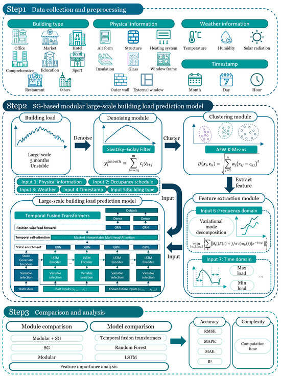
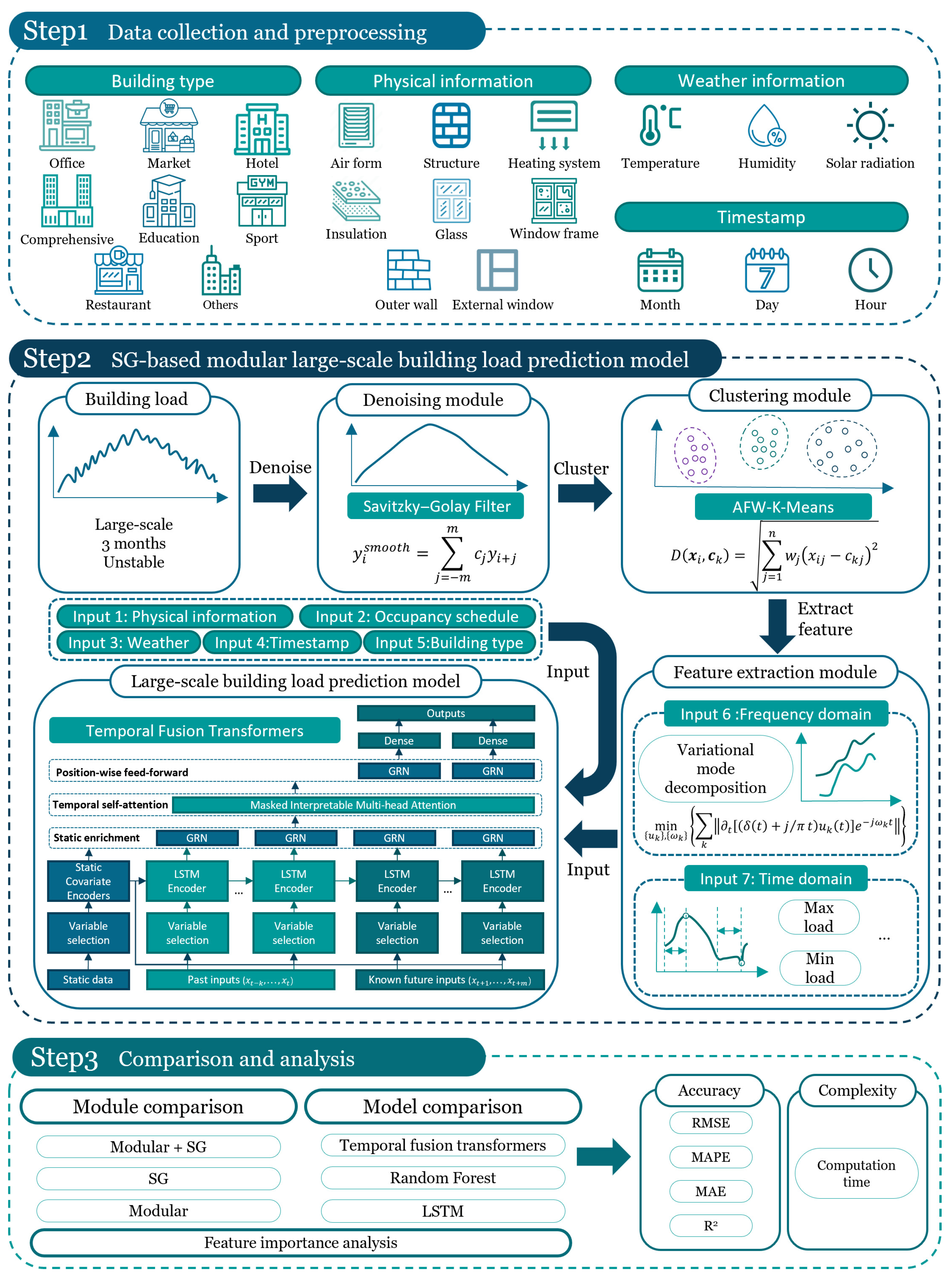
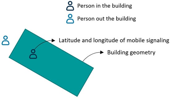
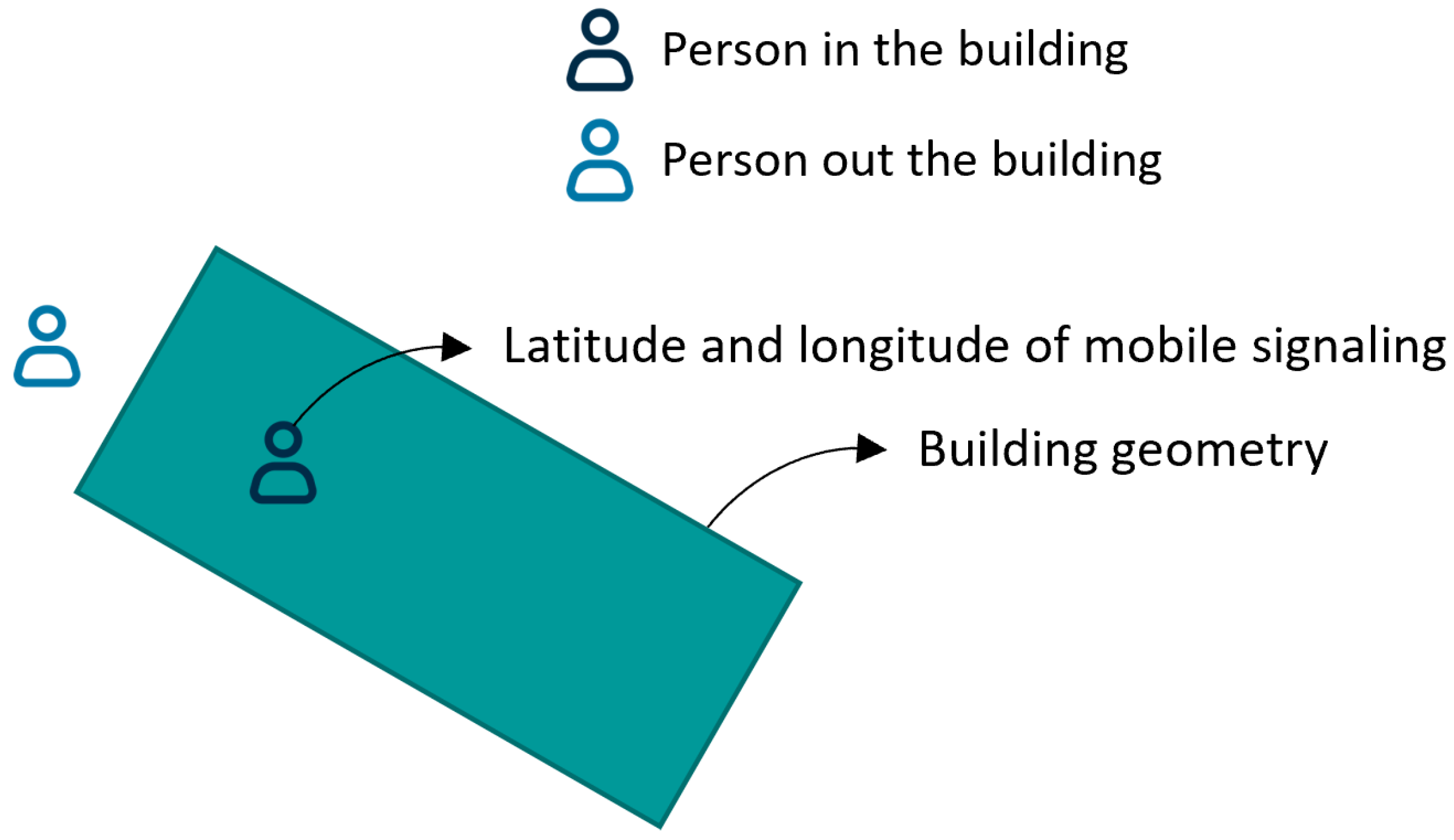
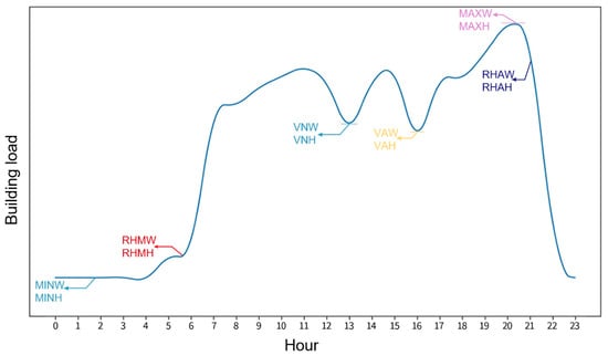
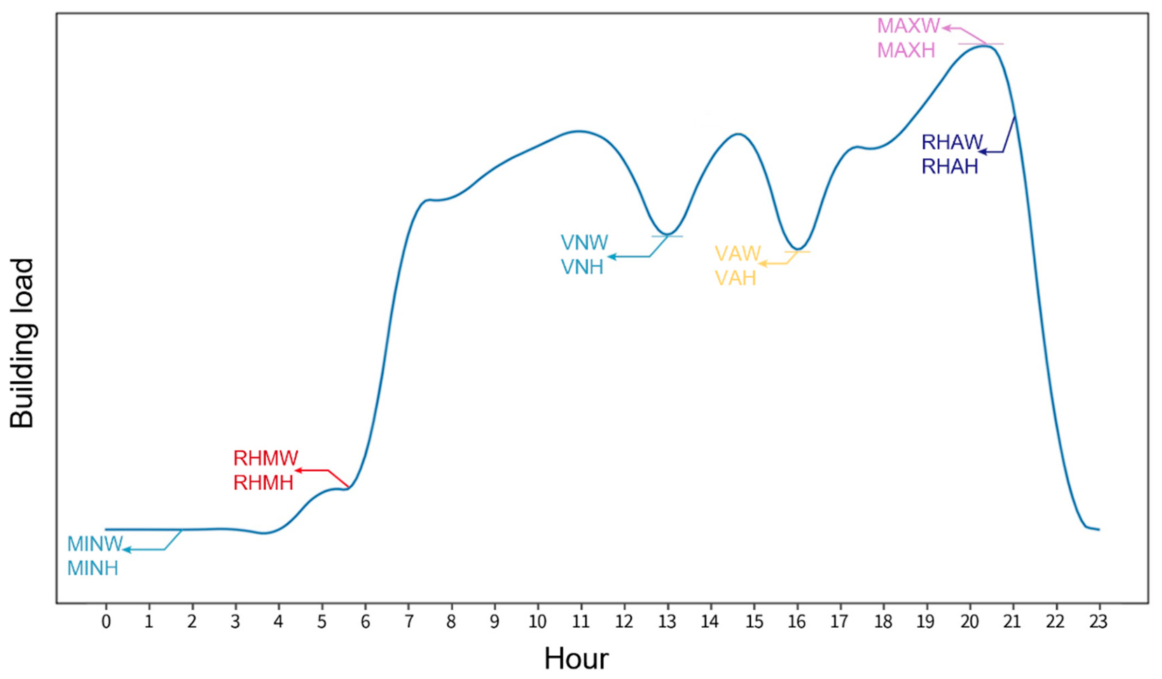
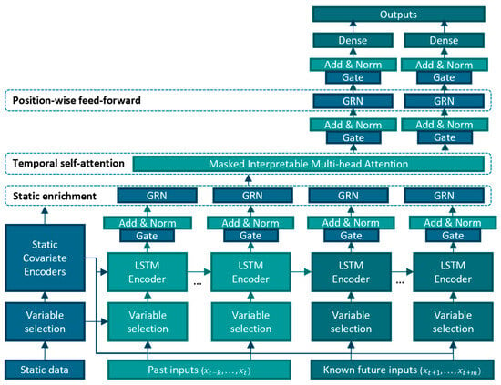
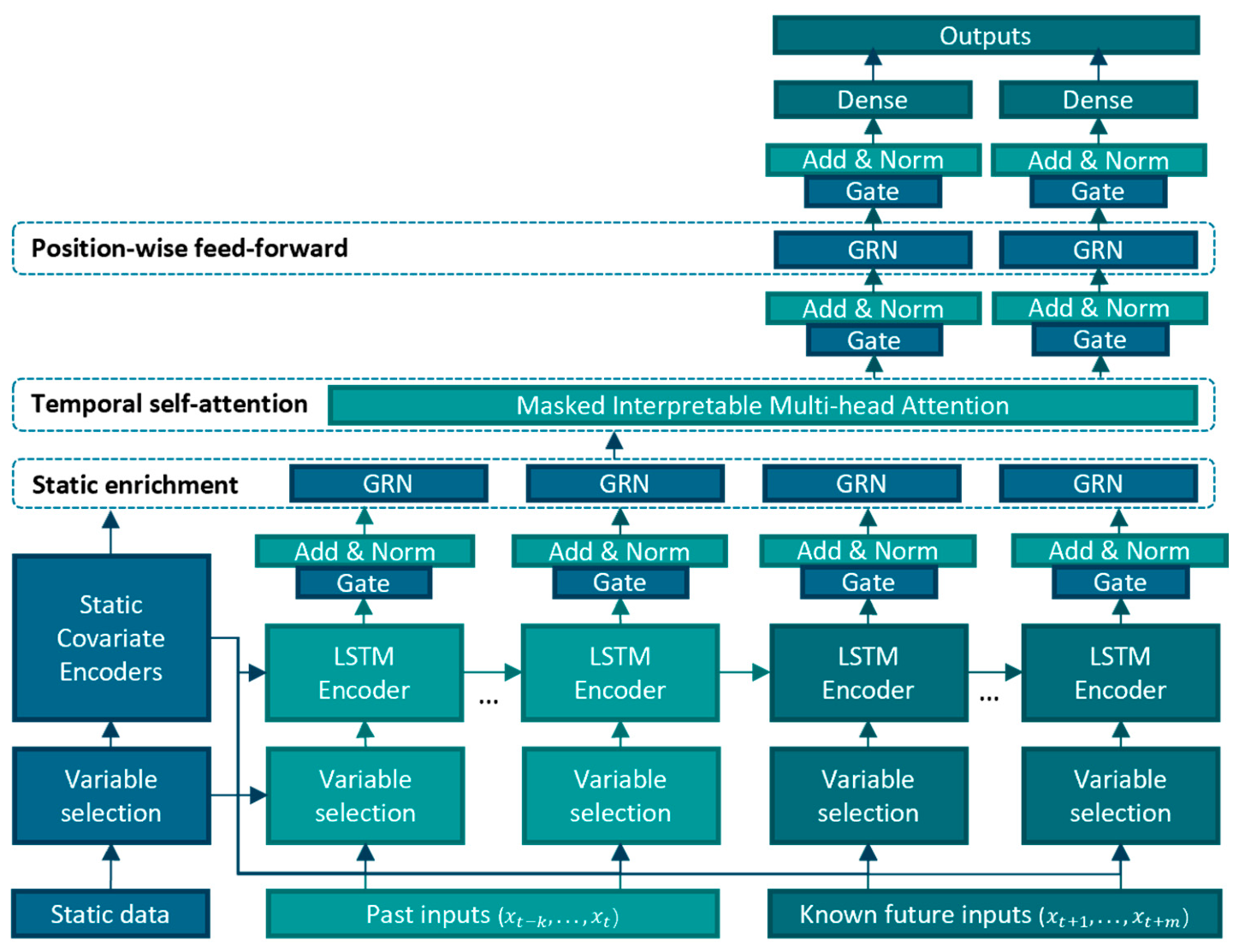
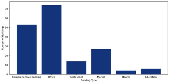
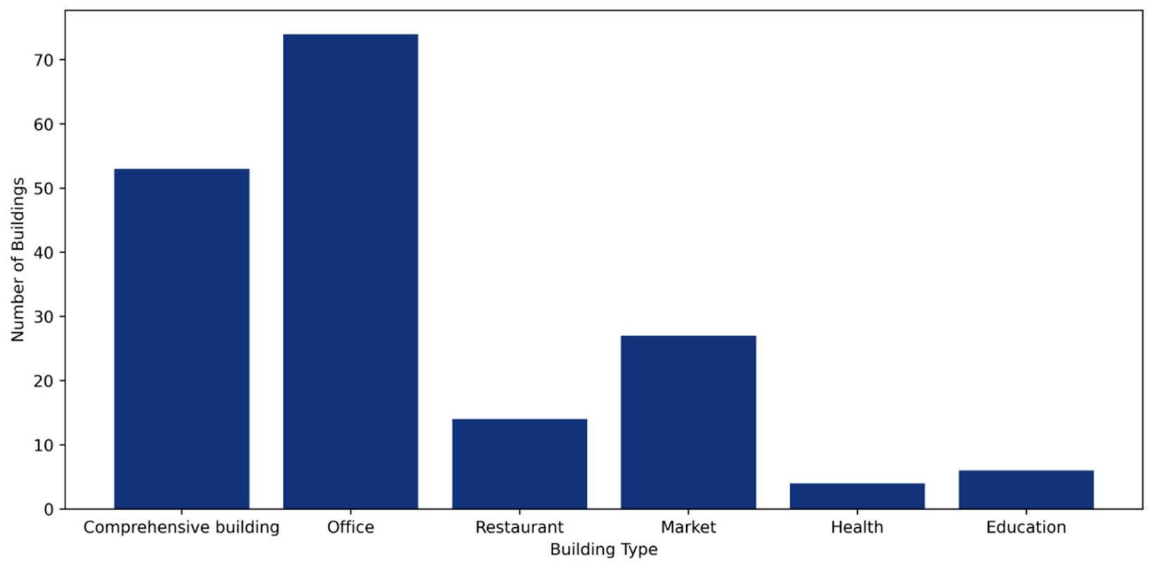
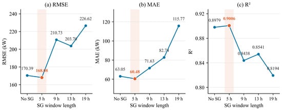
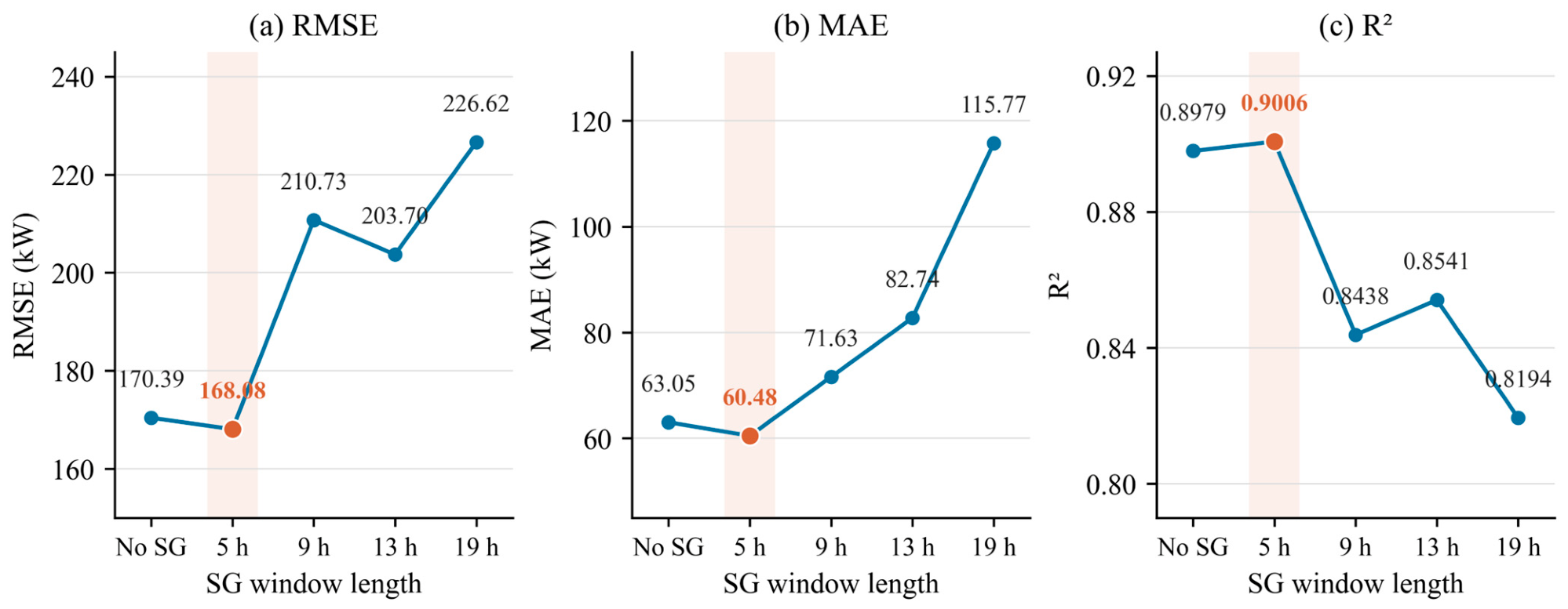
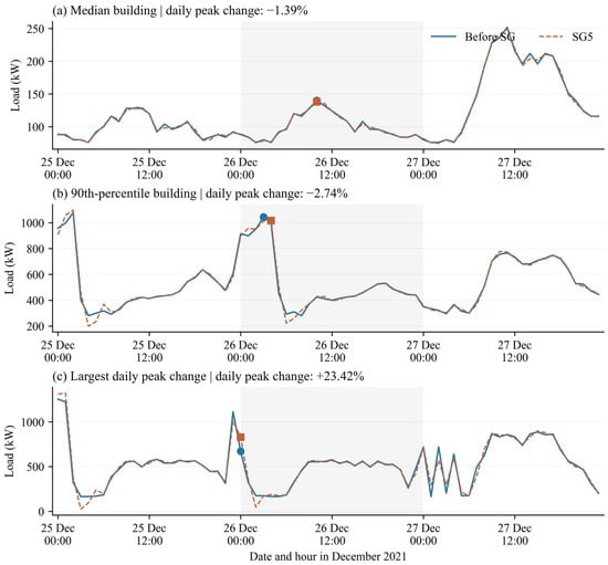
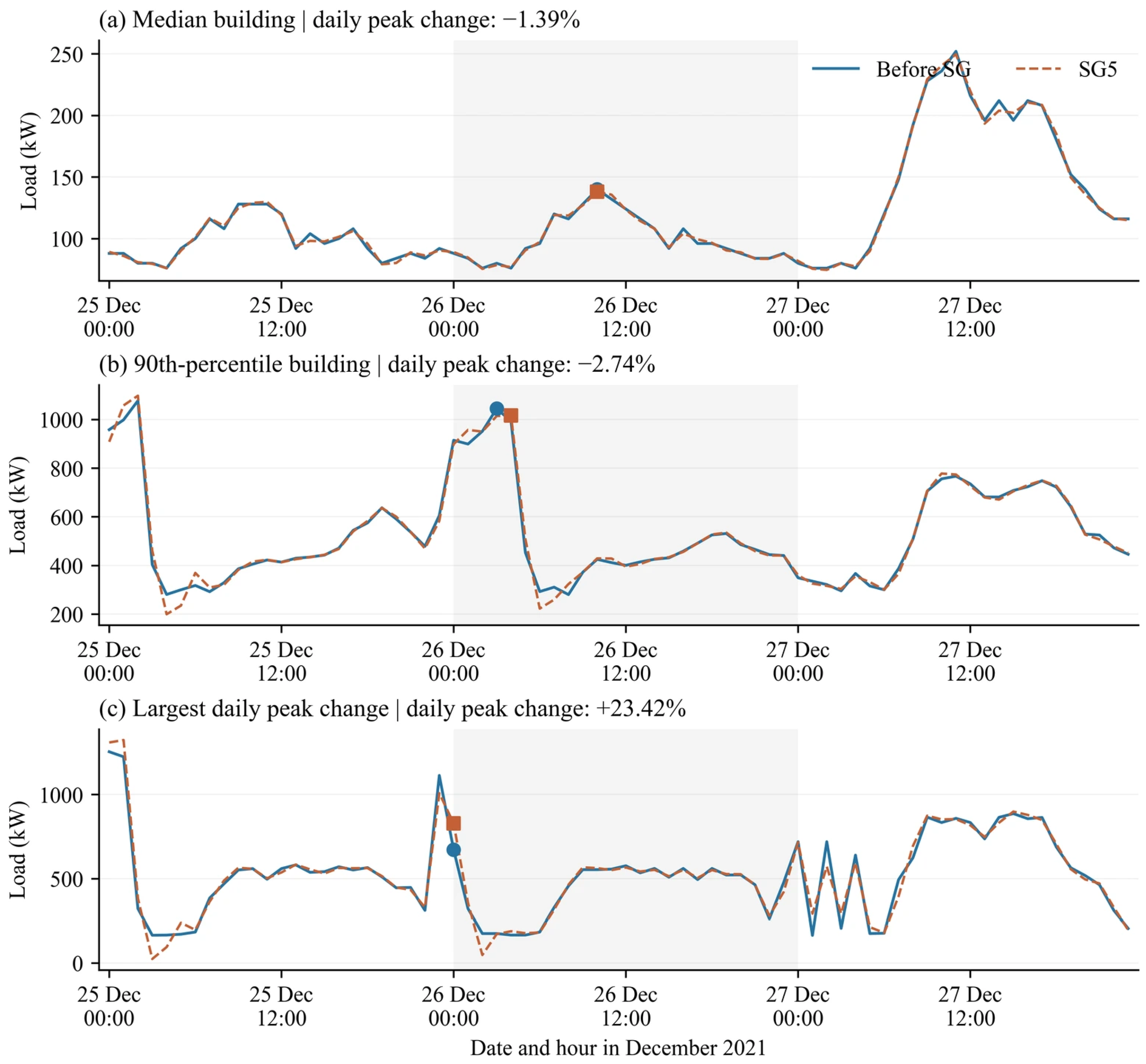
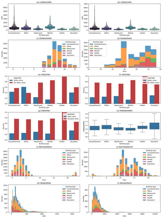
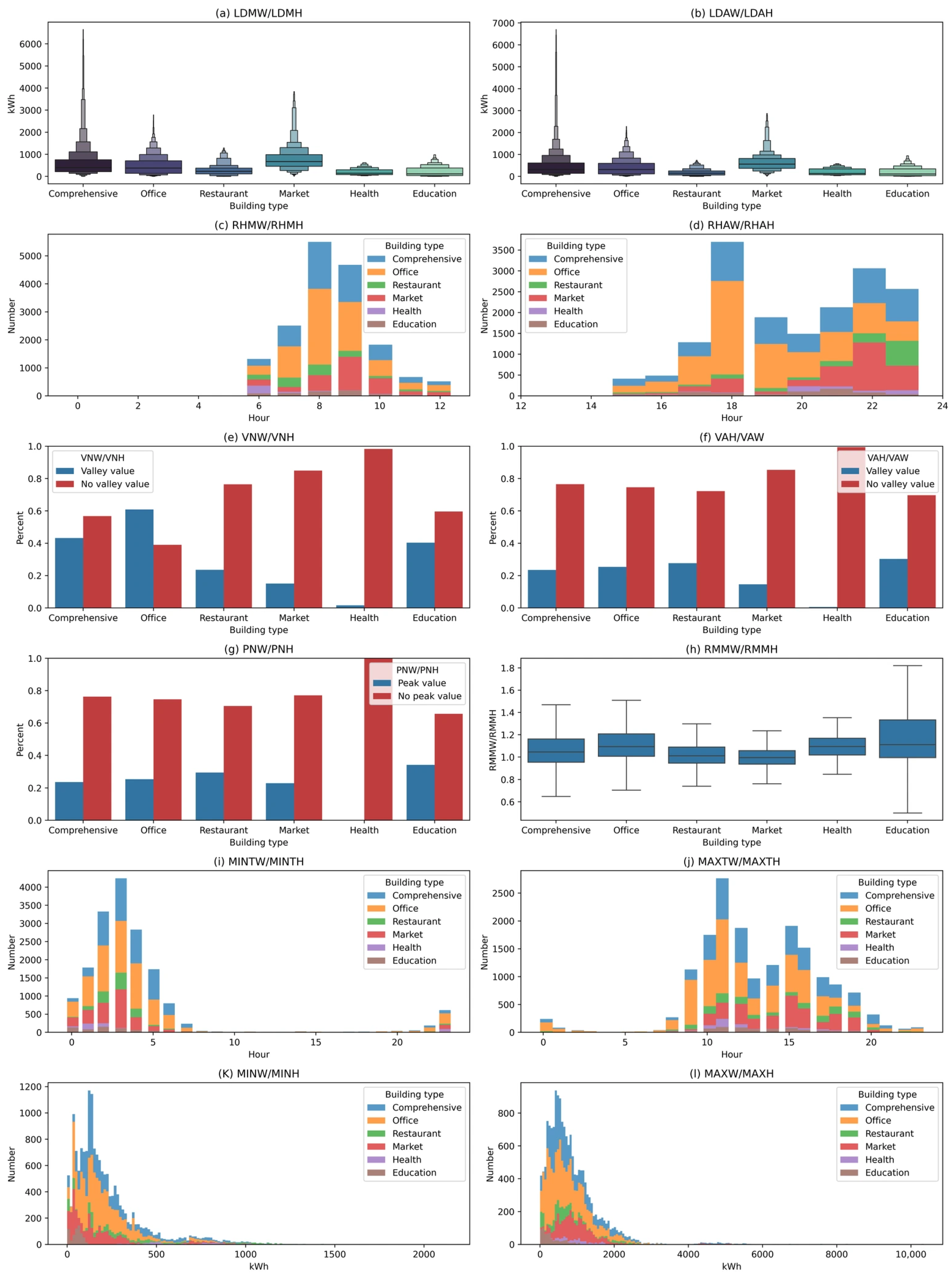
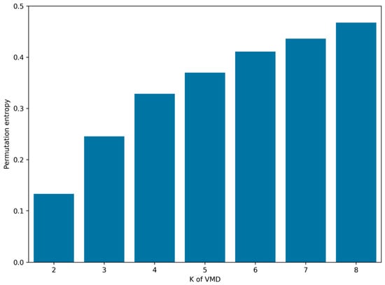
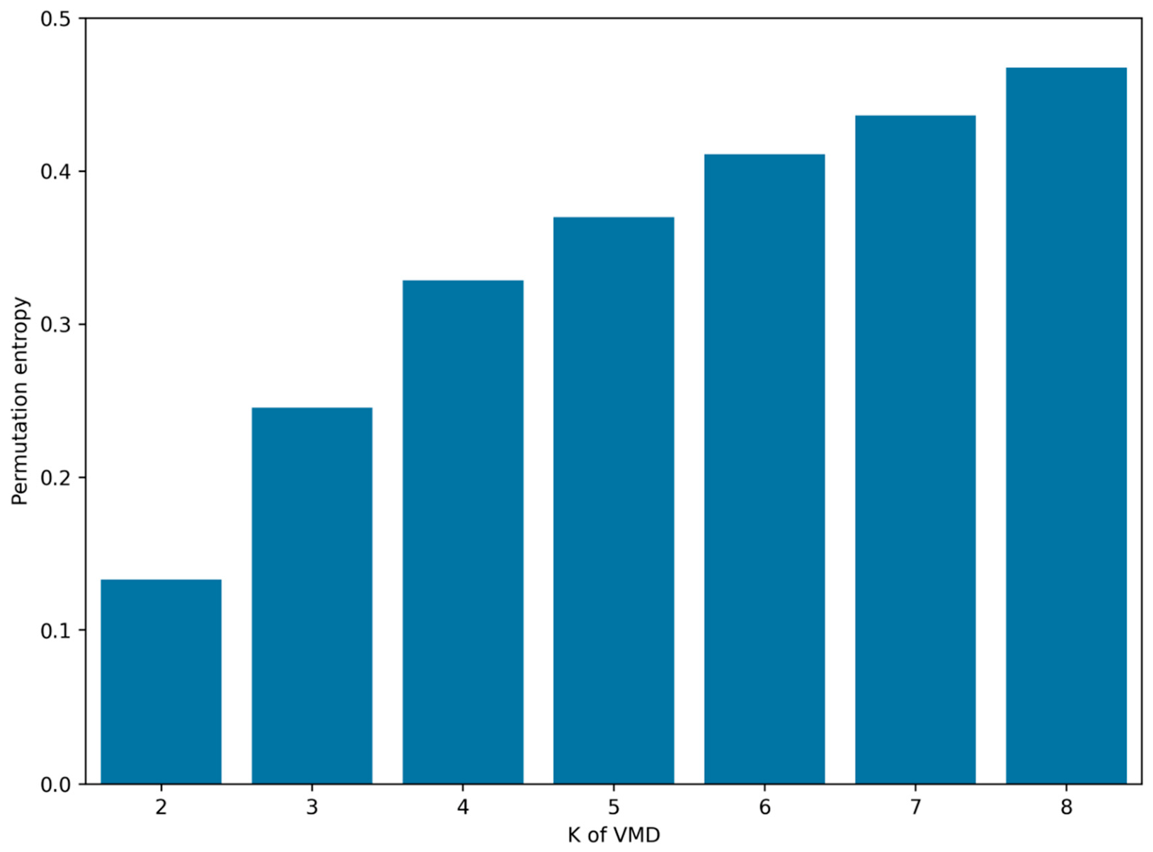
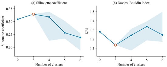
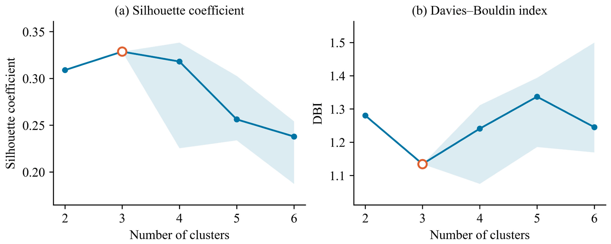
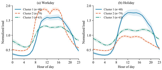
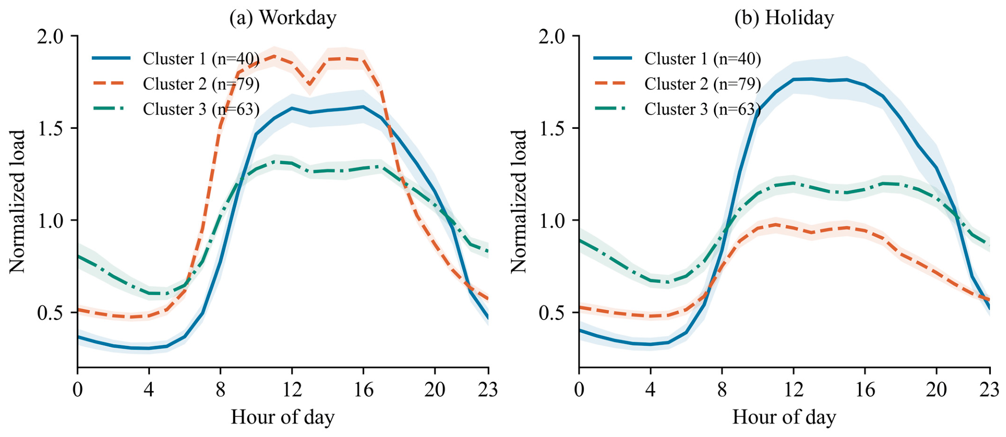
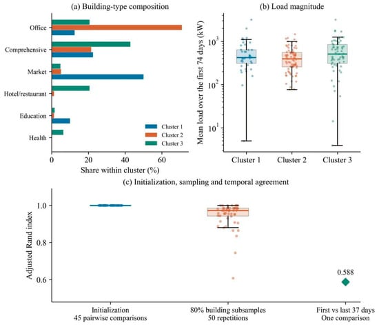
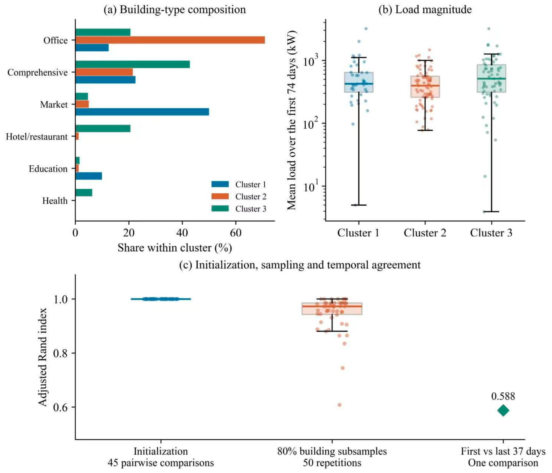
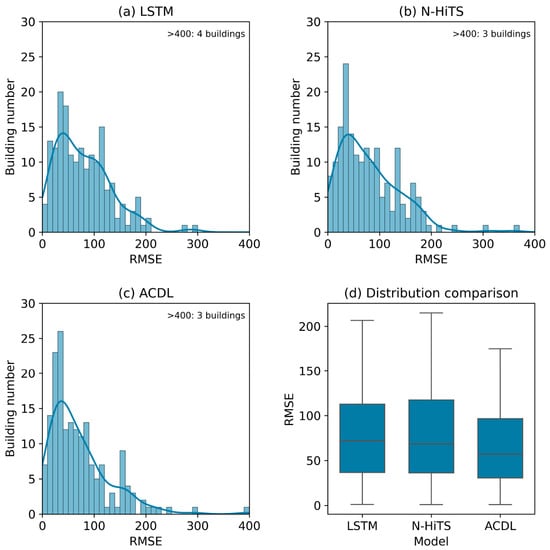
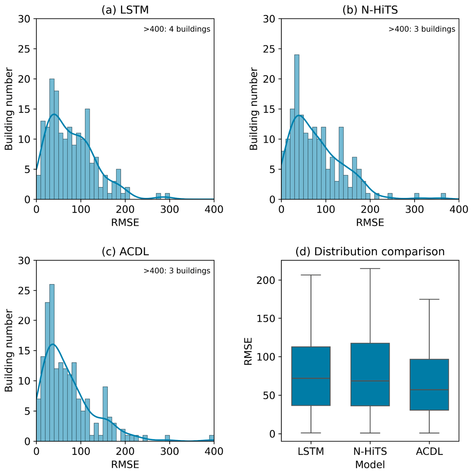
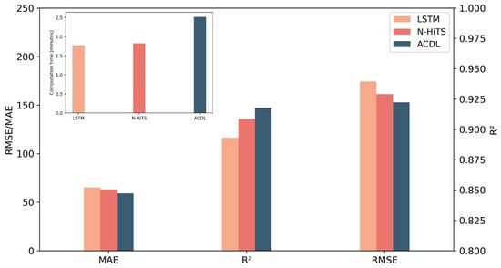
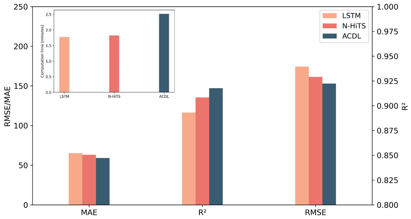
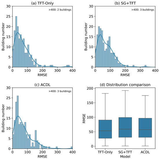
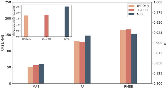
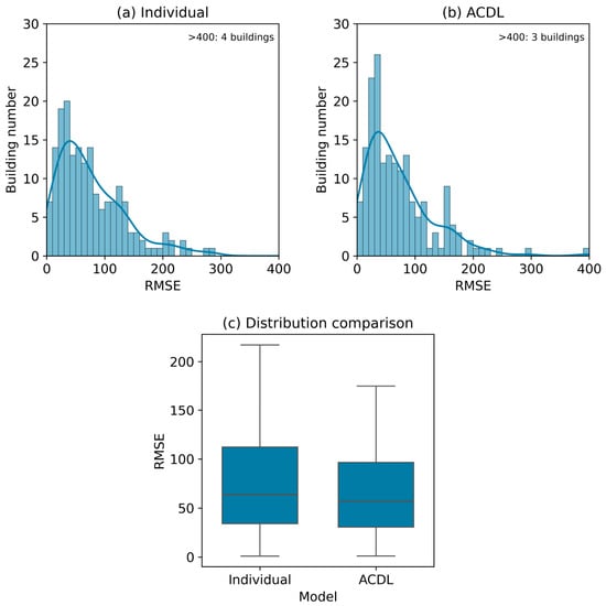
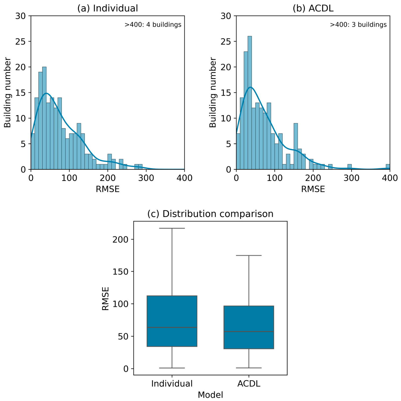
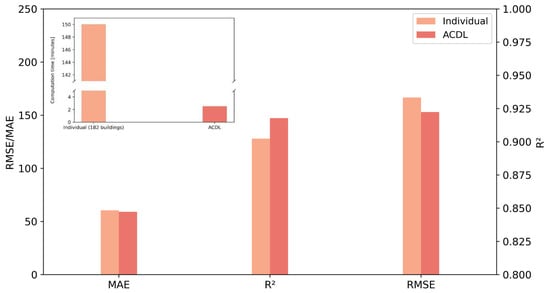
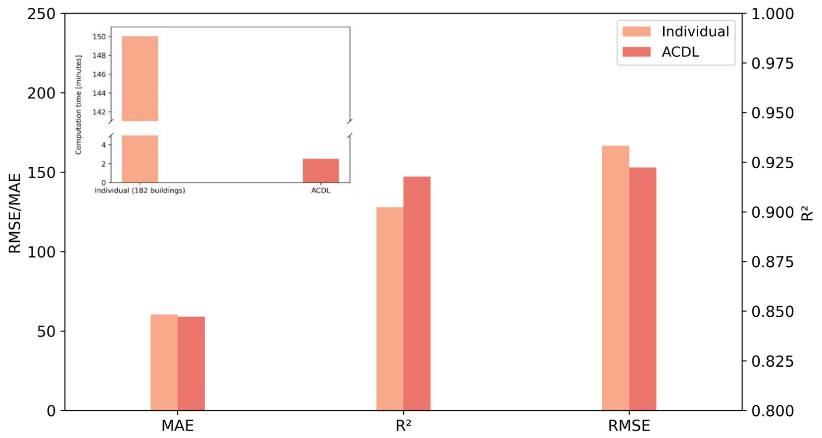
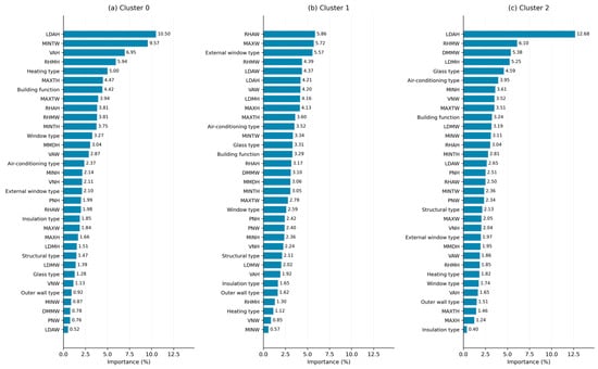
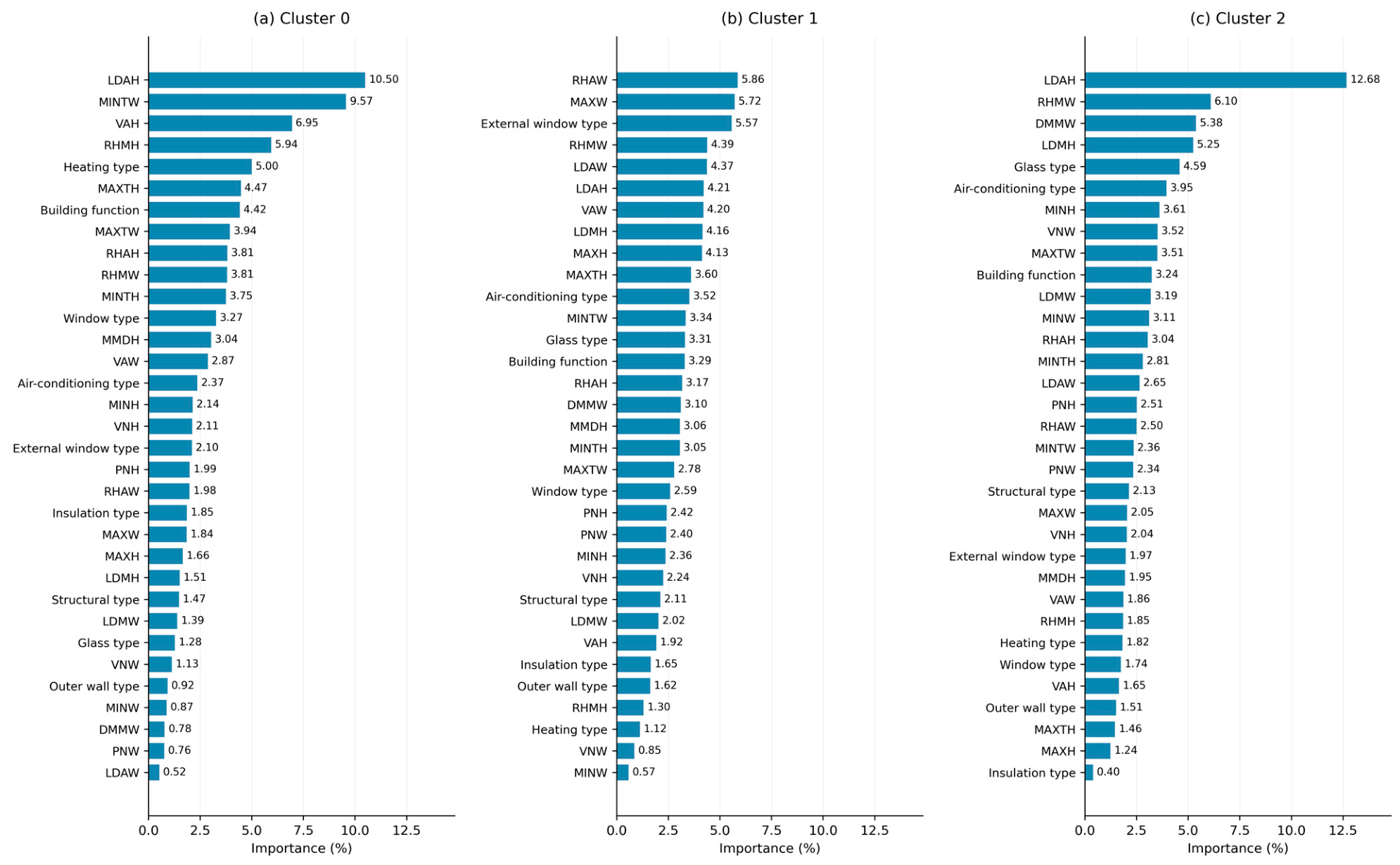
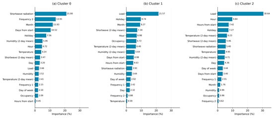
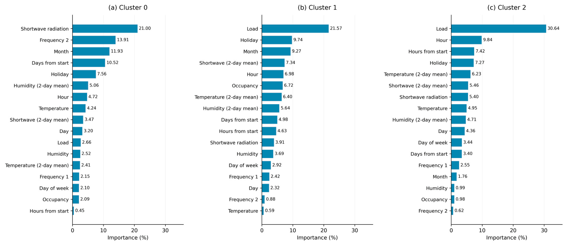
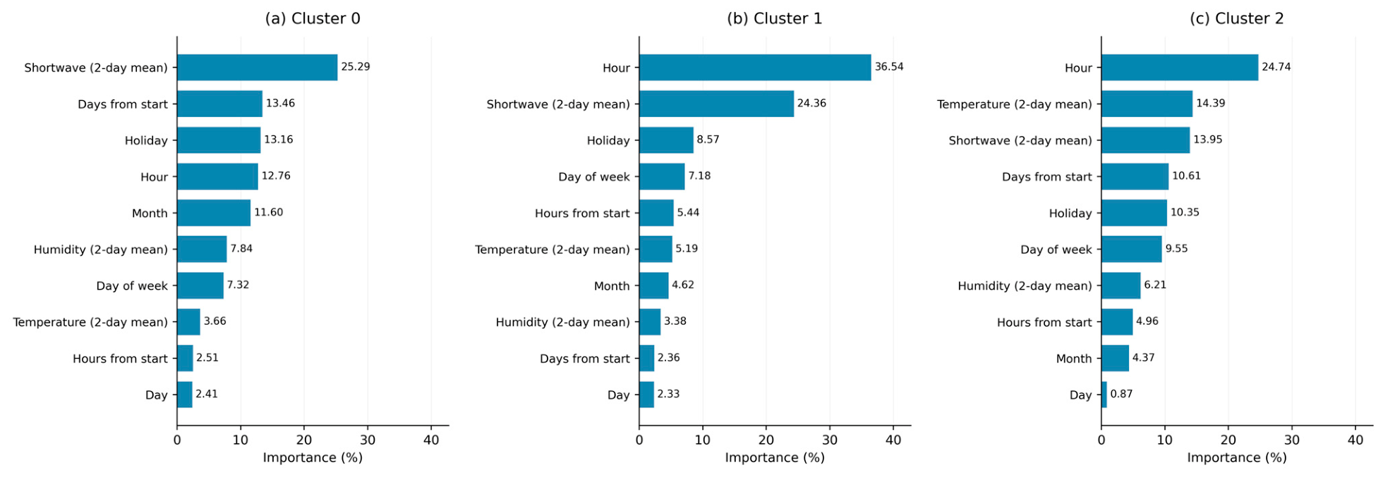

Disclaimer/Publisher’s Note: The statements, opinions and data contained in all publications are solely those of the individual author(s) and contributor(s) and not of MDPI and/or the editor(s). MDPI and/or the editor(s) disclaim responsibility for any injury to people or property resulting from any ideas, methods, instructions or products referred to in the content. |
© 2026 by the authors. Licensee MDPI, Basel, Switzerland. This article is an open access article distributed under the terms and conditions of the Creative Commons Attribution (CC BY) license.