


Abstract
In single-aspect studio apartments, daylight sufficiency and sunlight exposure constrain window design simultaneously. A studio reference room in Bangkok, Thailand was evaluated using Radiance through Ladybug Tools and a TMYx weather file. Six main-window configurations, three visible-light transmittance (VLT) levels (0.45, 0.65, 0.88), and four orientations formed a complete factorial set of 72 cases, assessed with spatial daylight autonomy (sDA300/50%), useful daylight illuminance (UDI100–3000), and annual sunlight exposure (ASE1000,250). The room was also simulated with the balcony door alone, giving a simulated baseline. Within the investigated design space, orientation accounted for 93.16% of the variation in ASE and 63.36% in UDI, but only 3.39% in sDA, which was governed instead by VLT (69.10%) and window configuration (23.23%). sDA ranged from 52.17% to 100.00% and 19 cases did not reach 75%; ASE ranged from 1.09% to 53.26%. The door alone gave a mean sDA of 47.10%, and the smallest window raised it by 25.00 percentage points. A screening rule informed by LEED v5 retained 29 cases and no west-facing case; substituting finer-grid values for four near-threshold cases reduced this to 28, testing that subset rather than grid independence across the dataset. Orientation and solar exposure should be assessed first, transmittance second, and window area last.
1. Introduction
Urban growth and vertical residential development have increased the prevalence of compact apartments in high-density cities. Studio apartments present a particular constraint because resting, dining, working, and personal activities occur within the same space. Working from home has further increased the importance of indoor environmental quality. Evidence gathered after the COVID-19 pandemic indicates that many dwellings were not designed to support daytime work and that lighting quality is one component of spatial suitability and occupant well-being [1,2,3,4].
Daylight contributes to vision, perceived spatial quality, satisfaction, and time-dependent physiological responses [5,6,7,8,9,10,11,12]. These benefits, however, depend not only on the quantity of light but also on its timing, distribution, spectrum, and variation between the window zone and the rear of a room. Experimental residential research has also associated daylight access with circadian alignment, sleep, and mental health [13]. A room with higher illuminance is therefore not necessarily of higher quality, particularly when illuminance frequently exceeds a useful range or when a large proportion of the floor area receives direct sunlight for prolonged periods.
Windows are the principal interface between outdoor sky conditions and the indoor luminous environment. Increasing the window-to-wall ratio (WWR), raising the window head or selecting glazing with a higher visible-light transmittance (VLT) can admit more light; however, the outcome also depends on orientation, room geometry, opening position, shading elements and external obstructions. Simulation studies across different climates do not support a single WWR or VLT value for every context and show that enlarging an opening can create trade-offs among daylight sufficiency, the proportion of time within a useful illuminance range, and direct sunlight exposure [14,15,16,17,18,19,20,21,22,23].
These constraints are particularly relevant in deep-plan, single-aspect spaces. Areas near the window may receive abundant light while the rear of the room remains dependent on daylight transmitted through the same set of openings. Recessed balconies, side walls, and upper slabs further reduce sky exposure. Studies of tropical dwellings, apartments, and deep-plan buildings show that orientation, room form, and depth materially alter daylight performance [16,17,24,25,26,27,28,29,30,31]. Research comparing WWR, window shape and position, and surrounding obstructions likewise confirms that glazing area alone cannot fully explain performance [18,19,20,21,22,23,32,33,34,35,36].
Climate-based daylight modeling (CBDM) combines hourly weather data with sky models and therefore represents temporal variation more comprehensively than the static daylight factor [37,38,39,40,41,42,43,44]. Spatial Daylight Autonomy (sDA) reports the proportion of an area that reaches a specified illuminance for a stated fraction of occupied time, whereas Annual Sunlight Exposure (ASE) reports the proportion exposed to direct sunlight above a specified threshold for an extended duration [38,39,45]. Useful Daylight Illuminance (UDI) characterizes the proportion of time for which illuminance falls within a useful range [46,47,48,49]. Because these metrics answer different questions and are sensitive to modeling assumptions, they should be interpreted together rather than using any single metric as a proxy for overall daylight quality [37,40,48,49,50].
Previous studies have investigated daylight performance in apartments and residential workspaces [2,3,16,23,24,25,26,27,28,29,30], as well as the effects of WWR, VLT, orientation and parametric design procedures [14,15,18,19,20,21,22,31,32,33,34,35,49,50]. Three gaps remain. First, the literature rarely distinguishes how additional glazing area is introduced: widening an opening, extending it upward, and extending it downward are usually aggregated into a single WWR variable, although each mechanism alters sky exposure and the geometry of the light path differently. Reporting these mechanisms separately, even along a sequence rather than under matched added areas, makes visible a distinction that a single ratio conceals. Second, orientation, window configuration, and VLT are frequently compared through group means without quantifying how much of the observed variation each factor explains, so statements such as “orientation is the dominant factor” remain qualitative. Third, studies that report sDA together with UDI and ASE rarely establish how much of the daylight in the room is already provided by apertures that the designer cannot remove. In compact residential units, a balcony access door is a fixed element, yet its contribution is normally absorbed into a single window-to-wall ratio. Without a simulated baseline for that aperture, the effect attributed to the main window is an increment on top of an unquantified starting point, and statements about how much additional glazing a room requires cannot be verified.
To address these gaps, this study used a single-aspect studio reference room under the climate of Bangkok as a parametric test bed. The study does not propose a universal window-size requirement and does not claim that the reference room represents all studio apartments.
This study asks how the variation in daylight sufficiency, useful illuminance, and sunlight exposure is distributed among room orientation, main-window configuration, and glazing transmittance in a single-aspect studio room, and how those three factors interact when a daylight-sufficiency criterion and a sunlight-exposure criterion must be satisfied at the same time. Because the six window configurations form a sequence with unequal baselines and unequal added areas rather than a matched-area set, the comparison between them is treated throughout as a description of change along that sequence, and not as an isolation of the effect of where glazing is added.
The study makes four contributions. First, it partitions the variation in three climate-based daylight metrics among orientation, window configuration, and glazing transmittance within a single complete factorial design, so that the relative influence of each factor is expressed as a share of the total variation rather than as a comparison of group means. Second, it reports an explicitly quantified simulation baseline for the fixed balcony access door: the room was simulated with that door as the only aperture across all four orientations and all three transmittance levels, which allows the contribution of each main-window configuration to be stated as an increment above a known starting point. Third, it reports the three mechanisms by which window area is increased separately rather than through a single window-to-wall ratio, while stating the limits of that comparison. Fourth, it reports how far the screening outcome depends on the resolution and placement of the analysis grid, by re-simulating the cases closest to the screening thresholds on a grid with four times as many points.
2. Materials and Methods
2.1. Reference Model and Scope of the Study
This study employed a controlled parametric simulation using a single-aspect studio apartment reference model under the climatic conditions of Bangkok, Thailand (13.73° N, 100.56° E). The model was established as a consistent test environment for examining the effects of window configuration, visible-light transmittance (VLT), and facade orientation. All other geometric, material, operational, and contextual parameters were held constant across the simulation cases, enabling direct comparison of the tested design variables.
The reference model was configured as a compact residential unit with a deep plan and daylight openings located along a single facade. Its principal dimensions were informed by the minimum spatial and ceiling-height requirements of Thai building regulations [51], while the depth relative to the facade width was selected to represent a daylight-constrained single-aspect condition. With a room depth of 7.30 m and a ceiling height of 2.70 m, the resulting depth-to-height ratio was 2.70, allowing the study to examine daylight penetration from the facade toward the rear of the unit. The model therefore represents a controlled design condition rather than a specific existing apartment. Accordingly, the findings are interpreted as comparative relationships within the investigated design space and should not be regarded as statistically representative of all studio apartments in Bangkok. Table 1 lists the fixed parameters of the reference room together with the basis for each value.
Table 1.
Fixed parameters of the single-aspect studio reference room and the basis for each value. Dimensions in meters.
The independent variables were six main-window configurations, three VLT levels, and four cardinal orientations, yielding a complete factorial set of 72 combinations (6 × 3 × 4). Because the 72 cases enumerate the entire defined design space rather than sampling from it, the analysis is deterministic: no sampling error exists, and inferential statistics such as p-values would have no defined meaning. Variation was therefore attributed to the factors by decomposing the total sum of squares (Section 2.8), which is the standard treatment of a full-factorial deterministic simulation experiment [52].
2.2. Spatial Organization and Fixed Openings
The interior comprised open, continuous pantry/dining, living, and bedroom zones, whereas the bathroom was modeled as an enclosed opaque volume. Two daylight openings were included, both in the same facade. The main window, Wx, was located in the living-zone wall flush with the building facade. A fixed glazed door, D1, measuring 1.80 × 2.00 m with a sill at 0.10 m and a head at 2.10 m, separated the bedroom from the balcony. D1 was recessed 0.95 m behind the facade and shaded by the upper slab and the side walls. Its geometry, position and fixed shading condition were unchanged in every case. Figure 1 shows the plan and the facade condition.
Figure 1.
Plan and facade condition of the reference room: (a) plan; (b) facade condition, showing the variable main window Wx, the recessed balcony, and the fixed glazed door D1 set back from the facade plane. In (a), solid lines denote physical walls and dashed lines functional-zone boundaries; the light-blue area comprises the pantry/dining, living, and bedroom zones covered by the analysis grid, and the gray areas are the bathroom and the balcony. In (b), x marks the dimensions of Wx that vary between configurations (Table 2). Dimensions in meters. The north arrow indicates the orientation shown; all four cardinal orientations were simulated by rotating the sky.
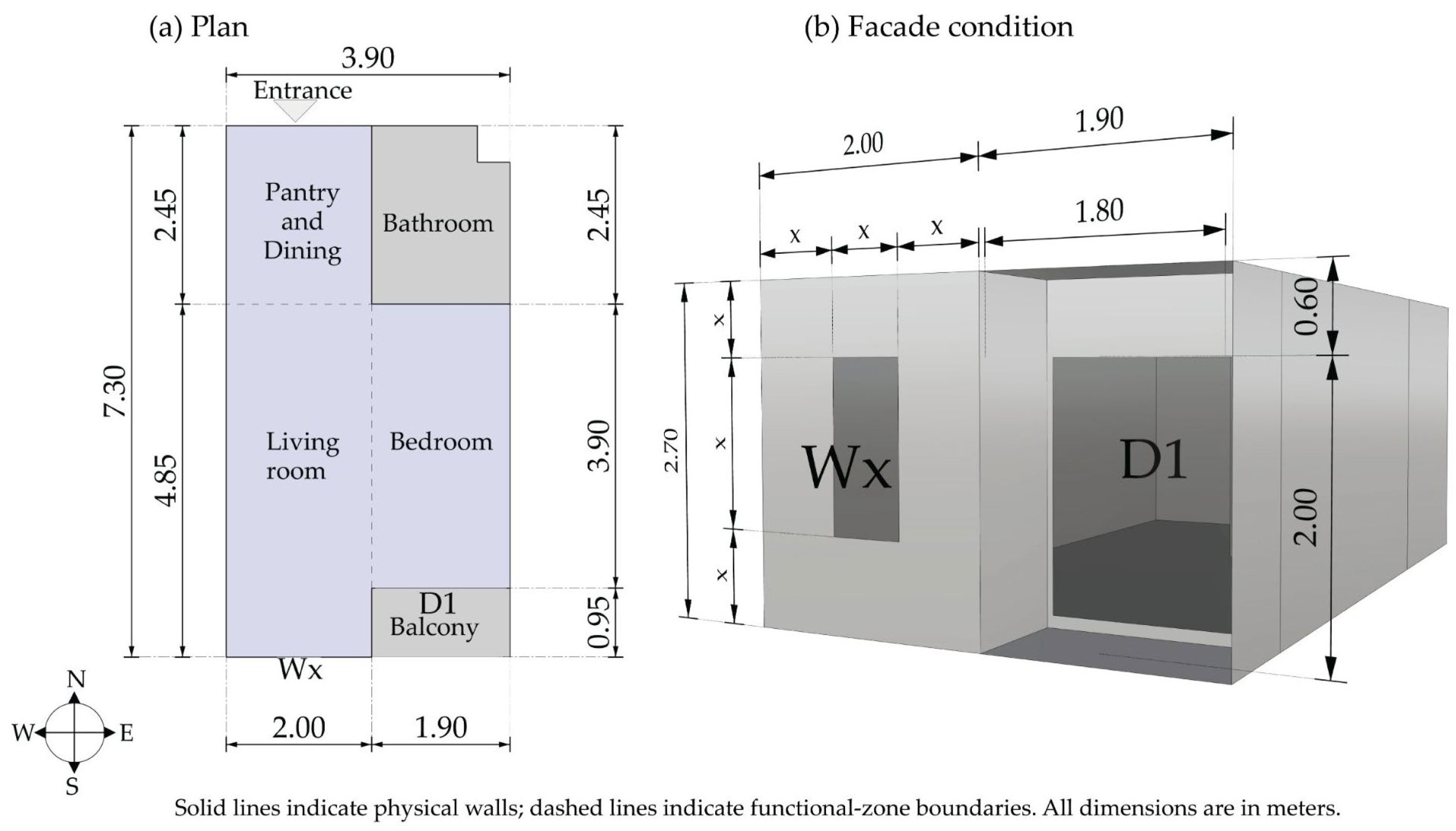
Table 2.
Dimensions and opening ratios of the six main-window configurations. The facade area is 3.90 × 2.70 m = 10.53 m2; the wall bay containing Wx is 5.40 m2; the fixed glazed door D1 contributes 3.60 m2 in every case.
2.3. Main-Window Configurations, Opening Ratios, and the Fixed Baseline Aperture
2.3.1. Window Configurations and Prespecified Comparisons
Windows W1–W6 were installed within a living-zone wall bay measuring 2.00 m wide and 2.70 m high, giving a bay area of 5.40 m2. Figure 2 shows the six configurations drawn within this bay, each with the fixed glazed door D1. Table 2 reports the dimensions of each configuration together with three distinct opening ratios, because a single “window-to-wall ratio” would be ambiguous in this geometry. The bay-glazing ratio expresses Wx as a fraction of the 5.40 m2 wall bay in which it is placed; it describes the local design move but is not a facade WWR. The facade WWR is reported twice: for Wx alone, and for Wx together with the fixed glazed door D1, since D1 is also a transparent element in the same facade. The window-to-floor ratio (WFR) is given relative to the 26.7 m2 enclosed interior because Thai regulation and much residential daylight guidance are expressed relative to floor area rather than wall area. Reporting the three ratios together prevents the different impressions that the three ratios create: the tested sequence spans a bay glazing ratio of 15.0–58.3% but a total facade glazed fraction of only 41.9–64.1%, because D1 already contributes 3.60 m2 of glazing in every case.
Figure 2.
Main-window configurations W1–W6 and the fixed glazed door D1, whose geometry and position were unchanged across all 72 cases. Drawn to scale within the 2.00 × 2.70 m wall bay; dimensions in meters. Dark gray areas are glazed openings, and light gray areas are opaque wall.
Three prespecified comparisons were defined along the W1–W6 sequence and are reported in Section 3.3. Group A compares W1 with W4, in which the width increases from 0.60 to 1.50 m while the height (1.35 m), the sill (0.75 m), and the head (2.10 m) remain constant. Group B compares W4 with W5, in which the head is raised from 2.10 to 2.55 m at constant width and sill. Group C compares W5 with W6, in which the sill is lowered from 0.75 to 0.45 m at constant width and head. The three comparisons are not matched in added area, so they describe change along one sequence and are not used to rank the three mechanisms.
2.3.2. Status of the Fixed Glazed Door as a Baseline Aperture
D1 was held constant deliberately, so that the six window configurations could be compared under an identical bedroom-side boundary condition. This choice has an important consequence that is treated as an explicit feature of the design rather than as an incidental detail. With an area of 3.60 m2, D1 is larger than every tested main window, and in the W1 case it supplies 81.6% of the total glazed area of the facade. The reference room therefore never approaches a minimally glazed condition: even the smallest main window sits on top of a fixed baseline supply of daylight, albeit one that is strongly shaded by the 0.95 m balcony recess, the upper slab and the side walls. This configuration was adopted because a balcony access door is a standard, essentially non-negotiable element of compact condominium units in the region, so a model without it would misrepresent the design problem. Because the door is present in every case, the effect of Wx reported here is an incremental effect relative to D1 rather than the effect of a sole aperture. The magnitude of that increment is not assumed: the room was simulated with D1 alone across all orientations and VLT levels, and the resulting baseline is reported in Section 3.8. Because the VLT of Wx and D1 was varied simultaneously (Section 2.4), the reported VLT effect is likewise a joint effect of two apertures with different shading conditions and cannot be attributed to either opening separately.
2.4. Optical Properties of Transparent and Opaque Surfaces
The transparent surfaces were assigned VLT values of 0.45, 0.65, and 0.88. These values were treated solely as optical parameters and were not assigned to commercial glazing categories or trade names because the relevant thermal properties—including emissivity, U-value, and solar heat gain coefficient—were outside the scope of this daylight study and were not modeled. The selected values represent low, intermediate, and high visible-transmittance conditions without being associated with specific glazing products. Within each case, the VLT values assigned to Wx and D1 were varied simultaneously. Consequently, the tested VLT levels represent changes to the glazing of the entire facade, and the effects attributed to VLT should not be interpreted as arising from the main window alone.
The Radiance glass modifier requires transmissivity as an input rather than visible transmittance. The corresponding transmissivities, calculated using the standard Radiance conversion, were 0.491, 0.708, and 0.958 for VLT values of 0.45, 0.65, and 0.88, respectively. Opaque surfaces were modeled using the plastic modifier, with diffuse reflectances of 0.50 for the walls, 0.20 for the floor, and 0.70 for the ceiling. The exterior ground and balcony floor were assigned a reflectance of 0.20. Table 3 summarizes these optical properties. Throughout this paper, each case is identified by its window configuration, VLT, and orientation (e.g., W1-VLT0.45-N); the same naming convention is used in Table S1 of the Supplementary Materials.
Table 3.
Optical properties assigned to transparent and opaque surfaces. Each transmittance level was applied to both Wx and D1.
2.5. Simulation Platform, Weather Data, and Boundary Conditions
The model was developed in Rhinoceros 8 and Grasshopper (both Robert McNeel & Associates, Seattle, WA, USA) using Ladybug Tools (lbt-gh) 1.9.4 (Ladybug Tools LLC, Fairfax, VA, USA) and the Honeybee Annual Daylight workflow coupled with Radiance 5.4a (Lawrence Berkeley National Laboratory, Berkeley, CA, USA). Radiance was selected on the basis of previous validation of daylight simulation engines and parametric workflows [37,40,41,49,50,53,54]. The present study did not include field measurements or a case-specific convergence test, and evidence from the literature is not treated here as a substitute for validation of this particular model.
Weather data were taken from the file THA_CRG_Bangkok.Metropolis.484550_TMYx.epw, obtained from Climate.OneBuilding.Org [55] and downloaded on 31 July 2026. This is the full period-of-record TMYx dataset for WMO station 484550, assembled from NCEI ISD and ERA5 sources over the period 1949–2025, rather than the shorter recent-period variant offered for the same station. The station coordinates were 13.7264° N and 100.5600° E, with time zone UTC+7 and an elevation of 4 m. The file was converted to the Radiance. wea format at an hourly timestep for the annual daylight calculation. A Perez all-weather sky was used [42]. The occupancy schedule was 08:00–18:00 every day of the year, totaling 3650 h, so that every case was assessed on an identical temporal basis. This schedule corresponds to the daytime period used in the LM-83 framework and in a study of residential workspaces in Bangkok; it is a controlled comparative schedule rather than a representation of any particular household [25,45].
The Annual Daylight simulations used the Radiance parameter string -ab 6 -ad 5000 -as 2048 -ar 300 -aa 0.1. In the Annual Daylight component this string replaces the recipe default (-ab 2 -ad 5000 -lw 2e-05 -dr 0) in full rather than being merged with it, so the limit-weight parameter was not set by the authors. Inspection of the rcontrib command lines recorded in the simulation folder confirms that -lw was not passed to the ray-tracing commands, which therefore used the Radiance default value of 2.00 × 10⁻³. The enhanced two-phase option of the Annual Daylight recipe was left at its default setting, which is active. The direct-sun contribution was therefore computed at each time step rather than distributed across a small number of sky patches, which is the setting appropriate for a metric defined on direct sunlight. ASE was derived from this direct-sun illuminance component of the recipe. The model included the recessed-balcony geometry and the fixed self-shading elements but excluded neighboring buildings, trees, furniture, curtains, blinds, and adjustable shading systems. The balcony balustrade was not modeled. The resulting unobstructed-sky condition represents a high sky-exposure boundary for comparative purposes and not a typical urban context; its implications are discussed in Section 4.6. Table 4 summarizes the simulation settings, and Figure 3 shows the Grasshopper implementation of the weather-file conversion and of the principal inputs of the Annual Daylight component. The four orientations were obtained by rotating the sky with the north_ input of the Annual Daylight component; values of 180°, 360°, 270°, and 90° place the facade containing Wx and D1 towards North, South, East, and West respectively, and each orientation was run in turn.
Table 4.
Simulation settings and boundary conditions for the 72 factorial cases and the 12 door-only baseline cases.
Figure 3.
Grasshopper implementation of the simulation workflow: (a) conversion of the EPW weather file to the Radiance WEA format; (b) principal inputs and orientation settings for the Honeybee Annual Daylight simulation. The version labels shown beneath the components refer to the individual component versions; the installed Ladybug Tools for Grasshopper version was 1.9.4.
2.6. Analysis Area, Sensor Grid, and Metric Resolution
The analysis grid was generated on a horizontal plane 0.75 m above the floor, which corresponds to the standard table height used in Thai residential interiors, over the full 3.90 × 7.30 m plan, using a nominal spacing of 0.48 m. Because the grid generator subdivides the surface into an integer number of cells, the resulting spacing was 0.4875 m in the x direction and 0.4867 m in the y direction. The 8 × 15 subdivision produced 120 grid positions. The 28 positions that fell in the bathroom or on the balcony, both outside the principal occupied area, were removed, and the remaining 92 points covered an analysis area of 21.83 m2 comprising the pantry/dining, living, and bedroom zones. Both spacings are below the 0.60-m maximum spacing recommended in the LM-83 framework [45]. This plane was used to assess daylight performance across the principal occupied area; it was not restricted to a single workstation and did not cover the full 26.7 m2 enclosed interior. Figure 4 shows the grid in plan and in three dimensions.
Figure 4.
Analysis grids on a horizontal plane 0.75 m above the floor: (a) the 92-point grid used for all 72 cases and for the door-only baseline, (b) the 368-point grid used for the resolution and placement test in Section 3.9, and (c,d) three-dimensional views of the same two grids. Nominal spacings of 0.48 m and 0.24 m give realized spacings of 0.4875 × 0.4867 m and 0.2438 × 0.2433 m, as explained in Section 2.6. Both grids cover the same 21.83 m2 analysis area; red dots mark the sensor points, and shaded areas are the bathroom and balcony, which were excluded.
The nominal value of 0.48 m was selected in preference to 0.50 m because the grid generator fits an integer number of cells across the 3.90 × 7.30 m plan. A nominal 0.50 m produces 7 × 14 cells and a realized spacing of 0.5571 m in x and 0.5214 m in y, which departs from the nominal value by 11.4% in x and yields cells 6.8% longer in one direction than in the other. A nominal 0.48 m produces 8 × 15 cells and a realized spacing that departs by 1.6% and is almost square, with an x-to-y ratio of 1.0017. The same reasoning applies to the finer grid: a nominal 0.24 m produces 16 × 30 cells, so the two grids are related by an exact factor of two in both directions and by a factor of four in point count. The resolution test is therefore not confounded by a change in cell proportion.
Because the sensor spacing was uniform, sDA and ASE were calculated from the proportion of the 92 analysis points without separately weighting boundary-cell areas. The reported values are therefore regular-grid point-count approximations of area proportions. One sensor point corresponds to 1.087 percentage points (pp), which is the resolution of sDA and ASE for an individual case: differences smaller than 1.087 pp cannot be resolved within a single case, although group means aggregated over 12 or 18 cases vary continuously. This quantization is stated explicitly because several of the endpoint differences reported in Section 3.3 are of that order, and it is a further reason for using Leadership in Energy and Environmental Design (LEED) as an interpretive reference rather than claiming full compliance with a standard. The consequences of this quantization for the screening outcome are examined directly in Section 3.9, where the cases lying closest to the screening thresholds were re-simulated on a finer grid.
To test whether the screening outcome depends on the resolution and placement of the sensor grid, a second grid was generated over the same plan using a nominal spacing of 0.24 m. This produced a 16 × 30 subdivision with 480 grid positions, of which the 112 falling in the same excluded regions were removed, leaving 368 points with a spacing of 0.2438 m in x and 0.2433 m in y over the same 21.83 m2 area, so that one point corresponds to 0.272 pp rather than 1.087 pp. Because each grid is generated independently and each point is placed at the center of its own cell, none of the 92 coarse-grid points coincides with a fine-grid point; the comparison therefore tests grid resolution and grid placement simultaneously. The cases selected for this test and the results are reported in Section 3.9.
For each case, Honeybee calculated hourly illuminance from skylight and sunlight over the complete occupancy schedule. Point-level results were summarized as sDA, UDI, and ASE and then aggregated to the case level. The same sensor points and schedule were used for every one of the 72 cases and for the door-only baseline, so that observed differences reflect window configuration, VLT, and orientation under otherwise fixed modeling conditions.
2.7. Metric Definitions
Let N = 3650 occupied hours, M = 92 analysis points, E(i,t) denote total illuminance at point i during hour t, and I(·) denote the indicator function. Daylight autonomy at 300 lx for each point was calculated as the proportion of hours for which E(i,t) ≥ 300 lx. The sDA300/50% value was then the percentage of points meeting this condition for at least 50% of occupied hours [38,39,45]:
sDA300/50% = (100/M) Σi I[(100/N) Σt I(E(i,t) ≥ 300 lx) ≥ 50%]
At each point, UDI100–3000 was the proportion of hours for which 100 lx ≤ E(i,t) ≤ 3000 lx; the case-level value was the mean across all 92 points. This interval distinguishes hours within the useful range from those below 100 lx or above 3000 lx [46,47,48]:
UDI100–3000 = (100/MN) Σi Σt I(100 lx ≤ E(i,t) ≤ 3000 lx)
ASE1000,250 was the percentage of points receiving more than 1000 lx of direct solar illuminance, Edir(i,t), for more than 250 occupied hours per year [45]. The definition and the inequality signs follow the Honeybee post-processing procedure used to generate this dataset:
ASE1000,250 = (100/M) Σi I[Σt I(Edir(i,t) > 1000 lx) > 250 h]
ASE indicates prolonged direct sunlight exposure on the horizontal analysis plane. It is a proxy for the potential for visual discomfort, not a measure of discomfort glare: no view-dependent metric such as Daylight Glare Probability was computed in this study, and no claim about perceived glare is made anywhere in this paper. This restriction is stated here, and again in Section 4.6, because ASE and glare metrics are frequently conflated in the applied literature. This is a strict inequality: a point that receives direct illuminance above 1000 lx for exactly 250 occupied hours is not counted. The convention follows the Honeybee implementation, in which the target-hours input specifies the number of hours that may not be exceeded.
Because sDA and ASE are derived from point counts, their attainable values on the 92-point grid are exact multiples of 1.087 pp. The second decimal place reported for these metrics therefore records exact arithmetic on the point count and should not be read as an independent level of simulation precision.
2.8. Variance Decomposition, LEED v5 Reference, and Screening Rule
The analysis first reported the minimum, maximum, mean, and population standard deviation (SDpop) across the 72 cases, together with means by window, VLT and orientation. SDpop is used rather than the sample standard deviation because the 72 cases constitute the entire defined design space and not a sample drawn from it.
To quantify the relative influence of the three factors, the total sum of squares of each metric across the 72 cases was decomposed into components attributable to the three main effects (orientation, window configuration, VLT), the three two-way interactions and the three-way interaction term. Each component is reported as its share of the total sum of squares, denoted η2. Because the design is a complete factorial with one deterministic observation per cell, the decomposition is exact and exhaustive, and the shares sum to 100%. This is a variance-based attribution of a deterministic simulation experiment rather than a statistical test: no error term, F statistic, or p-value is defined or reported, and the shares describe how the tested factors partition variation within this design space only [52]. They should not be read as sensitivity indices for a wider population of rooms, since they depend on the ranges chosen for each factor.
Effects for Groups A–C were additionally reported as differences between prespecified endpoints, both in percentage points and per square meter of added window area, to describe the magnitude of change. Dividing by added area does not place the groups on equivalent geometric baselines and was therefore not used to establish a universal ranking of the mechanisms.
For contemporary interpretation, the study referred to LEED v5 BD+C, EQc2 Occupant Experience, Option 5, Path 4: Daylight Simulation, which assigns daylight simulation levels at mean sDA300/50% values of at least 40%, 55%, 65%, and 75% [56]. Because this study assessed one room rather than all regularly occupied floor area in a project, its results are described as comparable to an sDA reference level without claiming LEED points or project certification. LEED v5 refers to ANSI/IES LM-83-23 and requires a glare-management approach to be identified where regularly occupied areas have ASEnet(1000, 250 h) > 20%; ASE is not used to remove sDA points automatically [56,57]. The ASE results reported here were produced by an Annual Daylight workflow based on the LM-83-12 framework and have not been verified as ASEnet under LM-83-23. The 20% level was therefore used as a comparative indicator and not as a claim of compliance.
For design-option screening, the primary study-defined rule was sDA300/50% ≥ 75% and ASE1000,250 ≤ 20%. This is a screening rule established by the authors with reference to the sDA level and the ASE indicator in LEED v5; it is not a LEED pass/fail criterion. A stricter sensitivity rule retained the same sDA condition while reducing the ASE threshold to ≤10%, showing how the retained set changed under the earlier, more restrictive threshold [45]. After retaining only cases that met the primary rule, the case with the highest UDI was selected within each orientation × VLT group; ties in UDI were to be resolved by lower ASE and then by smaller window area. UDI was treated as a continuous comparative metric with no universal pass threshold. Groups with no retained case were reported as such; no proxy case was created and no inference was extended beyond the studied design space.
All metric values are reported to two decimal places. Differences, ranges and per-square-meter ratios were computed from unrounded values and rounded once for reporting; they may therefore differ by 0.01 from the difference of the rounded entries shown in the same table.
3. Results
3.1. Overview of the Simulated Design Space
Across the 72 cases, sDA ranged from 52.17% to 100.00% with a mean of 80.01% and a population standard deviation (SDpop) of 10.72 pp (Table 5). Fifty-three of the 72 cases reached the 75% level and 19 did not. UDI ranged from 75.22% to 95.21% with a mean of 87.76% and an SDpop of 4.43 pp. ASE ranged from 1.09% to 53.26% with a mean of 20.92% and an SDpop of 16.90 pp; 43 of the 72 cases were at or below 20% and 21 were at or below 10%. The cases that did not reach the 75% sDA level were concentrated at the lowest transmittance: 16 of the 19 occurred at VLT 0.45 and the remaining three at VLT 0.65. By window configuration, seven occurred at W1, four at W2, four at W3, three at W4 and one at W5; none occurred at W6.
Table 5.
Descriptive statistics for the principal metrics across the 72 cases. SDpop is the population standard deviation, in percentage points.
The highest sDA, 100.00%, occurred in W6-VLT0.88-W and the lowest, 52.17%, in W1-VLT0.45-N. The highest UDI, 95.21%, occurred in W5-VLT0.65-N and the lowest, 75.22%, in W6-VLT0.88-W. The highest ASE, 53.26%, occurred in four west-facing cases, W5 and W6 at VLT 0.65 and 0.88, and the lowest, 1.09%, in seven north-facing cases, W1 and W2 at all three transmittance levels together with W3 at VLT 0.45. Although sDA reached 100.00% in one case, substantial variation remained across the investigated design space for all three metrics.
3.2. Relative Contribution of Orientation, Window Configuration, and VLT
Table 6 and Figure 5 report the decomposition of the total sum of squares of each metric. The three metrics were governed by different factors. Within the investigated design space, orientation accounted for 93.16% of the total variation in ASE and 63.36% in UDI, but only 3.39% in sDA. sDA was governed instead by VLT, which accounted for 69.10% of its variation, followed by window configuration at 23.23%. VLT accounted for 0.05% of the variation in ASE. Interaction terms were small throughout, with one exception: the window × VLT interaction accounted for 18.62% of the variation in UDI, compared with 1.98% for sDA and 0.01% for ASE.
Table 6.
Decomposition of the total sum of squares (SST) of each metric across the 72 cases. Values are the share of SST, η2, expressed as a percentage; the shares are computed before rounding and sum to 100%, so a printed row may total 99.99% or 100.01%. The decomposition is exact for a complete factorial design and is not a statistical test.
Figure 5.
Share of the total sum of squares of each metric attributable to orientation, window configuration, visible-light transmittance, and their interactions (O, W, and V denote orientation, window configuration, and VLT, respectively). Values as reported in Table 6.
The factor that dominates the sunlight-exposure risk is the one the designer usually cannot change late in the process, whereas the factor with the greatest influence on daylight sufficiency, glazing transmittance, remains adjustable late. The shares are conditional on the ranges tested here: had the window sequence extended to substantially smaller openings, or the VLT range been wider or narrower, the partition would differ. They describe this design space, not a general sensitivity ranking.
3.3. Effects of the Window-Area Increase Sequence
3.3.1. Increasing Main-Window Width (Group A)
Group A compared W1–W4, for which the width increased from 0.60 to 1.50 m while the height (1.35 m), sill (0.75 m), and head (2.10 m) remained constant. Averaged across orientations and VLT levels, changing from W1 to W4 added 1.215 m2 of window area, increased sDA from 72.10% to 81.52% (+9.42 pp), reduced UDI from 87.87% to 87.78% (−0.09 pp), and increased ASE from 14.67% to 22.10% (+7.43 pp). Normalized by the added area, Group A produced +7.75 pp sDA per m2 and +6.11 pp ASE per m2. Group A should not be read as inherently better or worse than the other groups, because it also had the largest increase in window area.
3.3.2. Extending the Opening Upward (Group B)
Group B compared W4 and W5. Width remained 1.50 m and the sill remained at 0.75 m while the head was raised from 2.10 to 2.55 m. The added area of 0.675 m2 increased mean sDA from 81.52% to 85.33% (+3.80 pp), reduced UDI from 87.78% to 87.07% (−0.71 pp), and increased ASE from 22.10% to 25.00% (+2.90 pp), corresponding to +5.64 pp sDA per m2 and +4.29 pp ASE per m2.
3.3.3. Extending the Opening Downward (Group C)
Group C compared W5 and W6. Width remained 1.50 m and the head remained at 2.55 m while the sill was lowered from 0.75 to 0.45 m. Adding 0.450 m2 increased sDA by 1.27 pp and reduced UDI by 0.13 pp, while mean ASE did not change, corresponding to +2.82 pp sDA per m2 and no measurable change in ASE per m2. This result is consistent with the added glazing lying largely below the analysis plane; the unequal baseline geometries, however, prevent causal attribution to sill lowering alone. W5 and W6 were also already the two largest windows, so the low position of the added glazing may have produced a different response from an equivalent addition to a smaller baseline window.
Within individual orientation × VLT combinations, sDA does not increase strictly monotonically across W1–W6. Ten of the sixty adjacent comparisons show a reduction, in every case, between 1.09 and 3.26 pp, corresponding to one to three analysis points. These reversals lie within the quantization described in Section 2.6, where a single sensor point corresponds to 1.087 pp. The grid-resolution test reported in Section 3.9 is consistent with this interpretation: for the W4–W5 pair at west and VLT 0.45, the reversal seen on the 92-point grid (76.09% and 75.00%) does not appear on the 368-point grid (73.91% and 77.99%), where a single point corresponds to 0.272 pp. The reported group means remain based on the common 92-point grid, and the finer-grid test did not alter the overall directional interpretation. Table 7 summarizes the three comparisons and Figure 6 shows the full W1–W6 sequence by orientation.
Table 7.
Prespecified group contrasts across the window-area increase sequence. Differences were computed from unrounded values.
Figure 6.
Mean (a) sDA300/50%, (b) UDI100–3000, and (c) ASE1000,250 across the W1–W6 window-area increase sequence, shown separately for each orientation (colored lines) and for all cases combined (black dashed line). The leftmost position, labeled D1 only, is the door-only baseline reported in Section 3.8; the gray dotted vertical line separates it from the W1–W6 sequence. In panel (a), the red dashed line marks the 75% sDA level used in both screening rules. In panel (c), the red dashed line marks the primary comparative indicator (ASE = 20%) and the red dotted line the sensitivity threshold (ASE = 10%).
3.4. Influence of Visible-Light Transmittance
Averaged across all windows and orientations, increasing VLT from 0.45 to 0.88 raised sDA from 68.70% to 90.49%, an increase of 21.78 pp. The effect on UDI was not monotonic: UDI was 87.46% at VLT 0.45, rose to 89.24% at VLT 0.65, and fell to 86.58% at VLT 0.88. Mean ASE changed by 0.91 pp across the same range, from 20.38% to 21.29%, which is consistent with the 0.05% share reported for VLT in Table 6. The pattern for UDI is consistent with the definition of the metric: at the lowest transmittance a larger share of occupied hours falls below 100 lx, and at the highest transmittance a larger share exceeds 3000 lx, so the intermediate level keeps more hours inside the interval than either extreme. ASE depends on the direct-sun component and classifies points by the number of threshold-exceeding hours, so a moderate change in transmittance rarely moves a point across both the 1000 lx and the 250 h conditions.
The number of cases retained under the primary rule differed markedly between transmittance levels: three of 24 at VLT 0.45, twelve of 24 at VLT 0.65, and fourteen of 24 at VLT 0.88. Under the sensitivity rule the counts were one, six, and seven. Transmittance was therefore the factor that differentiated the screening outcome most markedly, recognizing that VLT was changed simultaneously for Wx and D1. Table 8 and Figure 7 present the results by VLT level.
Table 8.
Mean performance and retained-case counts by VLT level. Each level comprises 24 cases; the screening rules are defined in Section 2.8. Both rules are study-defined; retention does not indicate compliance with LEED v5.
Figure 7.
Mean (a) sDA300/50%, (b) UDI100–3000, and (c) ASE1000,250 by VLT level, shown separately for each orientation (colored lines) and for all cases combined (black dashed line). Each value aggregates the six window configurations. In panel (a), the red dashed line marks the 75% sDA level; in panel (c), the red dashed line marks the primary comparative indicator (ASE = 20%) and the red dotted line the sensitivity threshold (ASE = 10%).
3.5. Influence of Room Orientation
Orientation produced the widest range in mean ASE and the narrowest in mean sDA. North had the lowest mean ASE (2.48%) and the highest mean UDI (92.78%); south had 12.50% and 88.25%; east had 22.28% and 87.16%; and west had the highest mean ASE (46.44%) and the lowest mean UDI (82.86%). The range between the highest and lowest orientation means was 43.96 pp for ASE and 9.92 pp for UDI. Mean sDA varied from 76.99% for north to 82.43% for west, a range of 5.43 pp. West therefore combined the highest mean sDA with the lowest mean UDI and the highest mean ASE, which is the central trade-off of this study.
Under the primary rule, 12 of the 18 north-facing cases, 14 of the 18 south-facing cases and three of the eighteen east-facing cases were retained; no west-facing case was retained. Under the stricter sensitivity rule the north-facing count was unchanged at 12, the south-facing count fell to two, and no east- or west-facing case remained. North was the only orientation for which tightening the ASE threshold from 20% to 10% removed no cases, because every retained north-facing case already had an ASE at or below 4.35%. Table 9 and Figure 8 summarize these results.
Table 9.
Mean performance and retained-case counts by room orientation. Each orientation comprises 18 cases. Both rules are study-defined, as in Table 8; retention does not indicate compliance with LEED v5.
Figure 8.
Mean (a) sDA300/50%, (b) UDI100–3000, and (c) ASE1000,250 by room orientation; the value above each bar is the mean of the 18 cases. Whiskers span the minimum and maximum of the 18 cases simulated for each orientation and do not represent confidence intervals. The red dashed line marks the 75% sDA level in (a) and the primary comparative indicator (ASE = 20%) in (c); the red dotted line in (c) marks the sensitivity threshold (ASE = 10%).
3.6. Trade-Offs Among Daylight Sufficiency, Useful Illuminance, and Sunlight Exposure
Figure 9 presents every case as a heatmap of UDI and ASE by orientation and window configuration at each VLT level, and Figure 10 plots UDI against ASE for all 72 cases. Two features are visible. First, the ASE panels are organized almost entirely by row: the north row remains at or below 5% in every window and VLT combination, while the west row exceeds 20% at every window, including W1. Second, within each orientation–VLT row, ASE generally increased or remained unchanged as window area increased, whereas UDI showed a non-monotonic response; variation across the three VLT levels remained comparatively smaller for ASE. In the trade-off plot, north-facing cases cluster at low ASE and high UDI, west-facing cases at high ASE and low UDI, and south- and east-facing cases occupy intermediate positions; separation by orientation is stronger than separation by VLT or by window area.
Figure 9.
Heatmaps of (a) UDI100–3000 and (b) ASE1000,250 for all 72 cases, arranged by orientation (rows) and main-window configuration (columns) at each VLT level (columns of panels). Values are percentages. N, S, E, and W denote north, south, east, and west; cell values are rounded to one decimal place, and the color bars give the scale for each row of panels.
Figure 10.
Trade-off between ASE and UDI across the 72 simulated cases. Color denotes orientation, marker shape denotes VLT, and marker size denotes main-window area, as identified in the legend. The red dashed vertical line is the comparative indicator informed by LEED v5 (ASE = 20%) and the gray dotted vertical line the stricter sensitivity threshold (ASE = 10%). Marker-size legend entries show the minimum and maximum main-window areas; intermediate areas are represented by proportionally scaled marker sizes.
Increasing the main window from W1 to W6 raised mean sDA by 14.49 pp and mean ASE by 10.33 pp, while mean UDI fell by 0.93 pp. Enlarging the window therefore improved daylight sufficiency at the cost of sunlight exposure rather than at the cost of the useful illuminance range. The general proposition that a larger window provides more daylight is supported in this design space, but it does not follow that enlargement is available in every orientation.
3.7. Study-Defined Screening and Selected Cases
3.7.1. Screening Results
Retention under the primary rule was determined by both conditions. Nineteen of the 72 cases did not reach the 75% sDA level and 29 cases exceeded the 20% ASE level; 29 cases satisfied both and were retained: 12 north-facing, 14 south-facing, and 3 east-facing. None of the tested west-facing cases satisfied both conditions. The term “retained” denotes conformity with the study-defined screening rule and does not mean that a case met LEED v5 requirements. The retained cases were distributed unevenly across the design space. For north and south, the number of retained cases increased with window area, from one and two cases at W1 to three cases each at W6, because the binding condition in these orientations was sDA. For east, cases were retained only at W1 and W2 and none at W3 or above, because the binding condition changed to ASE once the window exceeded 1.215 m2. For west, mean ASE at the smallest window was already 34.42%, above the 20% level before any enlargement was considered.
Under the sensitivity rule of sDA ≥ 75% and ASE ≤ 10%, the retained set decreased from 29 to 14 cases: 12 north-facing and two south-facing. No east- or west-facing case remained. The difference of 15 cases between the two thresholds shows that the choice and the communication of the ASE threshold directly affect design-screening outcomes, particularly for south and east orientations. By window configuration, the primary rule retained four cases at W1, six at W2, four at W3, four at W4, five at W5, and six at W6, whereas the sensitivity rule retained three, two, two, two, two, and three respectively. Figure 11 shows the retained counts by orientation.
Figure 11.
Number of retained cases under the primary study-defined rule and under the sensitivity rule, classified by orientation. Blue bars show the primary rule and orange bars the sensitivity rule. Eighteen cases were simulated per orientation, as marked by the gray dotted line.
3.7.2. Highest-UDI Cases Within the Retained Set
Within the retained set, the configuration giving the highest UDI depended on the transmittance level. At VLT 0.88, W1 gave the highest UDI for all three orientations with retained cases. At VLT 0.65, W5 gave the highest UDI for north, W3 for south, and W2 for east. At VLT 0.45, W6 gave the highest UDI for both north and south, and no case was retained for east or west. No group contained two cases with the same UDI, so the tie-breaking rule stated in Section 2.8 was not required. The dependence on transmittance follows from the sDA condition: at VLT 0.45 no case at W1, W2, or W3 reached the 75% level in any orientation, whereas at VLT 0.88 all 24 cases reached it, so the smallest window remained available. Table 10 lists the selected cases.
Table 10.
Highest-UDI cases within the sets retained by the primary rule. Dashes indicate groups with no retained case.
3.8. Daylight Provided by the Fixed Door Alone
The room was simulated with the balcony door D1 as the only aperture, across all four orientations and all three transmittance levels, giving twelve additional cases on the same 92-point grid. Mean sDA in this condition was 47.10%, ranging from 26.09% to 61.96%. No case reached the 75% level. Mean UDI was 77.44% and mean ASE was 9.24%; the door-only ASE was 0.00% for north-facing cases, and 23.91% for west-facing cases.
Adding the smallest main window, W1, raised mean sDA by 25.00 pp, and the increase ranged from 20.65 pp to 28.26 pp across the twelve orientation × VLT combinations. The corresponding increases for the larger configurations were 28.08 pp for W2, 32.25 pp for W3, 34.42 pp for W4, 38.22 pp for W5, and 39.49 pp for W6 (Table 11). The increment in ASE followed the same ordering, from 5.43 pp at W1 to 15.76 pp at W5 and W6. The increment in UDI was between 9.50 pp and 11.16 pp for every configuration and did not increase with window area.
Table 11.
Door-only baseline by orientation, and the mean increment produced by each main-window configuration relative to that baseline. The baseline comprises 12 cases.
Table 11 reports the baseline and the increments, and Figure 12 shows the increments for each metric. The fixed door therefore did not by itself bring the room to the sDA level used in the screening rule, and the contribution of the main window was substantial rather than marginal at every size tested.
Figure 12.
Mean increment in each metric produced by the six main-window configurations relative to the door-only baseline: (a) sDA300/50%, (b) UDI100–3000, and (c) ASE1000,250. Each bar is the difference between the mean of the 12 cases sharing a window configuration and the mean of the 12 door-only baseline cases, and is therefore averaged over the four orientations and three transmittance levels. The baseline value of each metric is stated above the corresponding panel. Values are in percentage points and correspond to those listed in Table 11.
3.9. Sensitivity of the Screening Outcome to Grid Resolution and Placement
Twelve cases lay within one sensor point of the 75% sDA level, the 20% ASE level or the 10% ASE level on the 92-point grid. These cases were re-simulated on the 368-point grid described in Section 2.6, which covers the same 21.83 m2 area at a resolution of 0.272 pp per point.
Figure 13 compares the two grids case by case. The mean absolute difference between the two grids was 1.38 pp for sDA, 0.84 pp for ASE and 0.58 pp for UDI; the largest differences were 3.53 pp, 2.17 pp, and 2.23 pp respectively. Four of the twelve cases changed classification (Table 12). Three changed at the sDA level: W1-VLT0.65-W crossed the sDA threshold on the finer grid, increasing from 73.91% to 75.82%, but remained unretained because its ASE was 35.33%. In contrast, W2-VLT0.65-N moved from 76.09% to 74.73%, and W4-VLT0.45-W from 76.09% to 73.91%, thereby crossing below the sDA threshold. One changed at the ASE level: W3-VLT0.45-E moved from 19.57% to 20.38%. Substituting the finer-grid values for these four cases changes the retained count under the primary rule from 29 to 28.
Figure 13.
Comparison of the twelve near-threshold cases on the 92-point and 368-point grids: (a) sDA300/50%, with the 75% sufficiency level shown as a red dashed line, and (b) ASE1000,250, with the 20% comparative indicator shown as a red dashed line and the 10% sensitivity threshold as a gray dotted line. Darker bars show the 92-point grid and lighter bars the 368-point grid. Red asterisks mark the four cases whose threshold classification changed on the finer grid. Values correspond to those listed in Table 12.
Table 12.
Comparison of the twelve near-threshold cases on the 92-point and 368-point grids. Cases lie within one sensor point (1.087 pp) of a threshold.
The cases that changed classification were those already identified as lying within one sensor point of a threshold. Only cases lying within one coarse-grid sensor increment of a threshold were re-simulated, so the test characterizes the sensitivity of near-threshold classifications rather than that of the full 72-case dataset. The ordering of orientations by retained-case count, and the finding that no west-facing case was retained, were unchanged. Because the differences between the two grids reached 3.53 pp for sDA and 2.17 pp for ASE, which exceed the 1.087 pp increment used to select the subset, the revised count of 28 is not demonstrated to be grid-independent across the full dataset.
4. Discussion
4.1. Orientation as the Principal Axis of the Trade-Off
The variance decomposition shows that the influence of orientation is metric-dependent. Within the investigated design space, orientation accounted for 93.16% of the variation in ASE and 63.36% in UDI, but only 3.39% in sDA. The common shorthand that orientation is the most important daylight variable is therefore accurate for sunlight exposure and for the useful illuminance range, but not for daylight sufficiency in this design space, where transmittance accounted for 69.10% of the variation and window configuration for 23.23%. Mean sDA differed by only 5.43 pp between the four orientations, compared with 43.96 pp for mean ASE. West combined the highest mean sDA with the lowest mean UDI and the highest mean ASE, while north had the lowest mean sDA together with the highest mean UDI and the lowest mean ASE. This pattern is consistent with studies showing that orientation and shading condition modify the effects of WWR and window design, and that a sufficiency metric alone cannot represent daylight quality [8,14,15,16,17,18,19,20,21,22,23,24,25,26,31,32,33,34,35,49,50].
These orientation differences occurred under a fixed single-aspect geometry with a recessed balcony. Wx was flush with the facade whereas D1 was recessed and shaded, so although the VLT of both openings changed simultaneously, their light paths and sky exposure differed. The results should not be reduced to the unqualified statement that north is best without specifying the balcony geometry, the room depth, and the unobstructed external context. A Bangkok studio-apartment study that assessed workstation locations reported a similar orientation ordering [25]; the present work differs by evaluating the complete 21.83-m2 principal occupied area, by distinguishing three window-area increase pathways and by quantifying the share of variation attributable to each factor.
4.2. The Fixed Aperture, the Increase Sequence, and the Two Binding Conditions
Simulating the room with the balcony door as the only aperture established a reference baseline against which the effects of the main-window configurations were evaluated. Across the 12 orientation × transmittance combinations, the door-only cases yielded a mean sDA of 47.10%, with all cases remaining below the study-defined 75% sufficiency criterion. Relative to this baseline, adding the smallest window increased mean sDA by 25.00 percentage points (pp), whereas adding the largest window increased it by 39.49 pp. These results show that the fixed glazed door alone did not meet the study-defined sDA criterion and that the main window made a substantial contribution across all tested configurations.
Along the W1–W6 sequence, mean sDA increased by 14.49 pp and mean ASE by 10.33 pp, whereas mean UDI decreased by only 0.93 pp. The three endpoint comparisons differed in magnitude: sDA increased across all three groups, whereas ASE increased in Groups A and B but showed no measurable change in Group C. Group A added 1.215 m2 of glazing and increased sDA by 9.42 pp and ASE by 7.43 pp; Group B added 0.675 m2 and increased sDA by 3.80 pp and ASE by 2.90 pp; and Group C added 0.450 m2 and increased sDA by 1.27 pp, with no measurable change in ASE. Because the three groups began from different baselines and involved different increments in glazing area, these comparisons describe changes along the W1–W6 sequence but do not isolate the effect of the position at which glazing was added. Accordingly, they should not be used to rank the relative effectiveness of the three opening-modification mechanisms.
The pattern of increments shows what is being exchanged. Calculated relative to the simulated door-only baseline, the gain in UDI was between 9.50 pp and 11.16 pp for every window size and did not increase with area, whereas the gain in sDA rose from 25.00 pp to 39.49 pp and the gain in ASE from 5.43 pp to 15.76 pp. Enlarging the window therefore improved daylight sufficiency at the cost of sunlight exposure rather than at the cost of the useful illuminance range. Group C illustrates the limit of this exchange: lowering the sill from 0.75 m to 0.45 m added 0.450 m2 of glazing and produced no change in mean ASE, a result consistent with the added glazing lying largely below the analysis plane, although the unequal baseline geometries prevent causal attribution to sill lowering alone.
The screening outcome is governed by two conditions that bind in different parts of the design space. For north and south, the binding condition was sDA: the number of retained cases increased with window area, and at VLT 0.45 no configuration below W4 reached the 75% level in any orientation. For east, the binding condition changed with window size, with cases retained only at W1 and W2. For west, neither enlarging the window nor changing the transmittance produced a retained case, because mean ASE at the smallest window was already 34.42%. The design space therefore contains a region in which the two conditions cannot be satisfied together, and that region is defined by orientation rather than by window size.
4.3. Role of VLT and the Limits of Glazing-Only Changes
Transmittance accounted for 69.10% of the variation in sDA, the largest single share for any factor and metric in this study apart from orientation in ASE. Raising VLT from 0.45 to 0.88 raised mean sDA by 21.78 pp and changed the number of retained cases from three to fourteen out of twenty-four. The effect on UDI was not monotonic: the intermediate level gave the highest mean UDI, because UDI is bounded at both ends and the lowest transmittance leaves more hours below 100 lx while the highest pushes more hours above 3000 lx.
Transmittance accounted for 0.05% of the variation in ASE, and mean ASE changed by 0.91 pp across the tested range. This should be read as a limited influence of transmittance on the ASE metric within the tested range, and not as evidence that transmittance is irrelevant to direct solar exposure itself. ASE classifies each point by the number of hours exceeding a fixed illuminance threshold, so a moderate change in transmittance rarely moves a point across both the 1000-lx and the 250-h conditions. In addition, the transmittance of the main window and the door was varied together, so the reported effect is that of the whole facade rather than of the main window alone. Because glazing thermal properties, color rendering, and view quality were not evaluated, no recommendation on a specific glazing product and no quantification of energy trade-offs can be drawn from these results.
4.4. Interpretation of LEED v5 and Sensitivity to the ASE Threshold
The LEED v5 framework distinguishes two issues that are often conflated. Daylight Simulation points are derived from sDA levels, whereas ASEnet > 20% prompts the identification of a glare-management approach and does not automatically remove sDA points [56,57]. It would therefore be incorrect to state that 29 cases passed LEED v5. The present study reports only that 29 cases met an author-defined screening rule informed by the LEED v5 sDA level and the ASE indicator.
Changing the ASE threshold from 20% to 10% reduced the retained set from 29 to 14 cases, with the largest effect on south, but did not alter the conclusion that north had the lowest exposure and west the highest. The two thresholds affected the orientations differently: for north, tightening the threshold removed no cases, because every retained north-facing case already had an ASE at or below 4.35%, whereas for south the retained count fell from fourteen to two. The choice of threshold therefore matters most for the intermediate orientations and least for the orientation with the lowest exposure. Reporting both levels serves two purposes: the 20% value aligns the interpretation with the current reference framework, while the 10% value maintains comparability with earlier work based on LM-83-12 [45]. Transparent reporting of this sensitivity is more important than selecting the threshold that produces the clearest narrative. A central limitation remains that the dataset has not been verified as ASEnet under LM-83-23, so the study makes no claim of compliance with the newer standard; future work should rerun the model using the LM-83-23 procedure and quantify the difference before applying such results in project-level assessment.
4.5. Implications for Single-Aspect Studio-Apartment Design
Within the boundaries of this reference room, the decision sequence suggested by these results begins with orientation and the shading context, because that is where the exposure condition is decided and it is the factor least available for change later. Where the orientation permits a retained case at all, transmittance is the next most effective variable, since it accounted for the largest share of the variation in sDA. Window area is then adjusted to the level required by the sufficiency condition at the chosen transmittance, with ASE checked at each step. At VLT 0.88 the smallest window was sufficient in every orientation with a retained case; at VLT 0.45 no configuration below W4 reached the sufficiency level in any orientation. The window area required is therefore conditional on the transmittance selected, and cannot be recommended independently of it.
For west, no tested case satisfied both conditions. Because mean ASE at the smallest window was already 34.42%, the appropriate response is to change the type of design intervention rather than to search for a nominal best option within the same set. Subsequent tests should include external devices addressing low-angle sun, vertical fins, controllable curtains or blinds, changes in opening position, and neighboring-building context. These are hypotheses for further study and were not tested here.
The design sequence proposed here is derived from daylight metrics alone and should be applied together with thermal and energy assessment. Glazing area can affect solar heat gain and cooling demand, whereas the thermal implications of visible transmittance cannot be determined without associated properties such as the solar heat gain coefficient and the U-value, neither of which was modeled here. The high west-facing ASE observed in this study, 46.44% on average, indicates prolonged exposure to low-angle afternoon sun, but its effect on cooling load was not quantified. No energy trade-off can therefore be inferred from these results.
The relevance to working from home lies in the multiple activities supported by a studio apartment and the longer periods occupants may spend indoors during daylight hours. A recent review characterized indoor environmental quality for homeworking as a multidimensional issue [4]. The present results should therefore be used as one daylight layer alongside thermal, acoustic, air-quality and behavioral considerations, rather than treating sDA, UDI, and ASE as a complete representation of indoor environmental quality.
4.6. Limitations and Future Research
First, the study examined one reference-room geometry. It did not sample buildings and did not vary room depth, facade width, floor level, or balcony form, so the conclusions are limited to a single-aspect room of 3.90 × 7.30 m with a 0.95-m deep recessed balcony and a fixed 1.80 × 2.00-m glazed door.
Second, the fixed door D1 was retained in every case and was not itself a variable. Its contribution was quantified explicitly through simulation (Section 3.8), but the two apertures were not varied independently, so the reported effect of transmittance remains a whole-facade effect. A design in which the two apertures are varied independently would separate these contributions.
Third, only the four cardinal orientations were simulated. Intercardinal orientations, particularly south-west and north-west, may produce exposure patterns that differ from those of the four cardinal orientations. Their performance cannot be inferred reliably from the present dataset and should be evaluated in future work.
Fourth, the external environment excluded neighboring buildings, trees, and reflective urban surfaces, so sDA may represent an upper bound relative to obstructed sites. Obstructions may also reduce ASE, although the direction and magnitude depend on their geometry, distance, and reflectance [22,36].
Fifth, the study included neither field measurements nor a model-specific convergence test. Although Radiance and related parametric workflows have been validated in earlier work [37,40,41,49,50,53,54], future studies should test sensitivity to ambient bounces and ambient divisions and compare simulated illuminance with measurements for representative cases.
Sixth, the daily 08:00–18:00 schedule was adopted for controlled comparison and does not represent every household. Restricting occupancy to working days, extending it into the evening or modeling blind operation could change UDI and ASE.
Seventh, sDA and ASE were approximated as area proportions by counting 92 uniformly spaced grid points without weighting boundary-cell areas, giving a per-case resolution of 1.087 pp. The grid-resolution test in Section 3.9 showed that four of the twelve cases lying within one point of a threshold changed classification on a finer grid. Individual cases close to a threshold should therefore not be read as decisive, although the ordering of orientations and the absence of any retained west-facing case were unaffected. Studies aiming at strict standards assessment should use cell-area weighting or a grid subjected to sensitivity testing.
Eighth, no view-dependent metric was computed. ASE is a horizontal-plane proxy for prolonged direct sunlight and is not a measure of discomfort glare; conclusions about occupant glare perception would require Daylight Glare Probability or an equivalent view-based analysis, which is a priority for subsequent work on this room.
Ninth, the study addressed daylight only. It did not evaluate thermal performance, energy, cost, life cycle, outward view, or privacy, and the selection of window size and VLT in practice must integrate these considerations.
Finally, the balcony balustrade required by regulation was not modeled. A perforated or glazed guardrail would reduce the low-angle daylight and low-angle direct sun reaching the recessed door D1, so the values reported for the door-only baseline, and for the west-facing cases in particular, should be read as an upper bound in this respect.
5. Conclusions
This study evaluated the effects of six main-window configurations, three VLT levels (0.45, 0.65, and 0.88) and four orientations on sDA, UDI, and ASE in a single-aspect studio reference room under the climate of Bangkok, using a complete factorial set of 72 cases together with a door-only baseline of 12 cases.
Within the investigated design space, the three metrics were governed by different factors. Orientation accounted for 93.16% of the variation in ASE and 63.36% in UDI, but only 3.39% in sDA, which was governed instead by transmittance (69.10%) and window configuration (23.23%). The factor with the greatest influence on sunlight-exposure risk is therefore the one normally fixed earliest in the design process, while the factor with the greatest influence on daylight sufficiency is one that remains adjustable late.
sDA ranged from 52.17% to 100.00% and 19 of the 72 cases did not reach the 75% level; UDI ranged from 75.22% to 95.21% and ASE from 1.09% to 53.26%. The door alone gave a mean sDA of 47.10% and did not reach the 75% level in any orientation or at any transmittance. Adding the smallest main window raised mean sDA by 25.00 pp and the largest by 39.49 pp, while the gain in UDI was between 9.50 pp and 11.16 pp for every configuration. Enlarging the window in this room therefore improved daylight sufficiency at the cost of sunlight exposure rather than at the cost of the useful illuminance range.
All three endpoint comparisons produced an increase in sDA, though differing in magnitude; ASE increased in Groups A and B but showed no measurable change in Group C. Increasing width from W1 to W4 produced the largest changes; raising the head from W4 to W5 produced smaller changes; and lowering the sill from W5 to W6 produced the smallest increase in sDA and no measurable change in ASE. Because the comparisons had unequal baselines and unequal added areas, they describe change along this sequence and do not establish a universal ranking of window-enlargement methods.
The primary study-defined screening threshold retained 29 of 72 cases: 12 north-facing, 14 south-facing, and 3 east-facing. No west-facing case was retained at any window size or transmittance, because mean ASE at the smallest window was already 34.42% in that orientation. Tightening the exposure threshold from 20% to 10% reduced the retained set to 14 cases and removed no north-facing case. For the twelve near-threshold cases re-simulated on the finer grid, four threshold classifications changed, reducing the primary retained count from 29 to 28; the orientation ranking and the absence of retained west-facing cases were unchanged. Because only the cases lying within one coarse-grid increment of a threshold were re-simulated, and because the differences between the two grids reached 3.53 pp for sDA and 2.17 pp for ASE, this test demonstrates sensitivity for the selected subset and does not establish that the retained count of 28 is grid-independent across the full dataset. These results should not be described as cases passing LEED v5, because project-level certification was not assessed and the ASE values have not been verified as ASEnet under LM-83-23.
The window area required for a retained case depended on the transmittance selected. At VLT 0.88 the smallest window was sufficient in every orientation with a retained case, whereas at VLT 0.45 no configuration below W4 reached the sufficiency level in any orientation. The resulting design implication is to establish the orientation and assess its solar-exposure and shading context first, then select transmittance, and only then determine the window area needed at that transmittance, checking exposure at each step. This conclusion applies to rooms with geometry, occupancy, balcony conditions, and external context comparable to the reference room, and is not a window-size requirement for all apartments or climates.
Supplementary Materials
The following supporting information can be downloaded at: https://www.mdpi.com/article/10.3390/buildings16193883/s1, Table S1: Case-level results on the 92-point grid; Table S2: Case-level results for the twelve near-threshold cases on both grids; Table S3: Recipe input record for a representative simulation run.
Author Contributions
Conceptualization, N.N. (Nitchapha Naphatthakan); methodology, N.N. (Nitchapha Naphatthakan) and N.N. (Narisa Noithapthim); software, N.N. (Nitchapha Naphatthakan); validation, N.N. (Nitchapha Naphatthakan), N.N. (Narisa Noithapthim) and F.M.R.; formal analysis, N.N. (Nitchapha Naphatthakan); investigation, N.N. (Narisa Noithapthim); resources, N.N. (Nitchapha Naphatthakan); data curation, N.N. (Nitchapha Naphatthakan); writing—original draft preparation, N.N. (Nitchapha Naphatthakan); writing—review and editing, N.N. (Nitchapha Naphatthakan), N.N. (Narisa Noithapthim) and F.M.R.; visualization, N.N. (Nitchapha Naphatthakan); supervision, N.N. (Narisa Noithapthim) and F.M.R.; project administration, N.N. (Nitchapha Naphatthakan); funding acquisition, N.N. (Nitchapha Naphatthakan). All authors have read and agreed to the published version of the manuscript.
Funding
This research was funded by Walailak University under the Research Grant for New Researchers, fiscal year 2026 (B.E. 2569), grant number WU69223.
Data Availability Statement
The simulation input files and raw data supporting the findings and conclusions of this study are available from the corresponding author upon reasonable request.
Acknowledgments
The authors would like to acknowledge Walailak University for providing institutional support, research facilities, and academic resources that supported the completion of this study.
Conflicts of Interest
The authors declare no conflicts of interest. The funder had no role in the design of the study; in the collection, analysis or interpretation of data; in the writing of the manuscript; or in the decision to publish the results.
Abbreviations
The following abbreviations are used in this manuscript:
| ASE | Annual Sunlight Exposure |
| CBDM | Climate-Based Daylight Modeling |
| D1 | Fixed glazed door between the bedroom and the balcony |
| EPW | EnergyPlus Weather file |
| LM-83 | IES-approved method for sDA and ASE |
| pp | percentage points |
| SDpop | Population standard deviation across all studied cases |
| sDA | spatial Daylight Autonomy |
| SST | Total sum of squares |
| UDI | Useful Daylight Illuminance |
| VLT | Visible-Light Transmittance |
| WFR | Window-to-Floor Ratio |
| WWR | Window-to-Wall Ratio |
| Wx | Variable main-window configuration, W1–W6 |
| η2 | Share of the total sum of squares attributable to a factor |
References
- Cuerdo-Vilches, T.; Navas-Martín, M.Á.; Oteiza, I. Working from Home: Is Our Housing Ready? Int. J. Environ. Res. Public Health 2021, 18, 7329. [Google Scholar] [CrossRef] [Scilit] [PubMed]
- Acosta, I.; Campano, M.Á.; Bellia, L.; Fragliasso, F.; Diglio, F.; Bustamante, P. Impact of Daylighting on Visual Comfort and on the Biological Clock for Teleworkers in Residential Buildings. Buildings 2023, 13, 2562. [Google Scholar] [CrossRef] [Scilit]
- Mousavi, S.M.; Shokouh, S.; Mohammadi, A.; Hosseini Nasab, S. Assessing Daylighting Conditions and Strategies in Residential Workspaces During the COVID-19 Pandemic: A Case Study of Apartment Buildings in Malaysia. Int. J. Built Environ. Sustain. 2025, 12, 203–215. [Google Scholar] [CrossRef] [Scilit]
- Navas-Martín, M.Á.; Jiménez-Planet, V.; Cuerdo-Vilches, T. Working from Home and Indoor Environmental Quality: A Scoping Review. Appl. Sci. 2026, 16, 250. [Google Scholar] [CrossRef] [Scilit]
- Aslanoğlu, R.; Pracki, P.; Kazak, J.K.; Ulusoy, B.; Yekanialibeiglou, S. Short-term analysis of residential lighting: A pilot study. Build. Environ. 2021, 196, 107781. [Google Scholar] [CrossRef] [Scilit]
- Rastegari, E.; Adamsson, M.; Aries, M. Daylight potential of Swedish residential environments: Visual and beyond-vision effects and the relationship with well-being assessment. Light. Res. Technol. 2025, 57, 156–180. [Google Scholar] [CrossRef] [Scilit]
- Karaman Madan, Ö.; Chamilothori, K.; van Duijnhoven, J.; Aarts, M.P.J.; de Kort, Y.A.W. Restorative effects of daylight in indoor environments—A systematic literature review. J. Environ. Psychol. 2024, 97, 102323. [Google Scholar] [CrossRef] [Scilit]
- Yu, X.; Su, Y. Daylight availability assessment and its potential energy saving estimation—A literature review. Renew. Sustain. Energy Rev. 2015, 52, 494–503. [Google Scholar] [CrossRef] [Scilit]
- Acosta, I.; Campano, M.Á.; Leslie, R.; Radetsky, L. Daylighting design for healthy environments: Analysis of educational spaces for optimal circadian stimulus. Sol. Energy 2019, 193, 584–596. [Google Scholar] [CrossRef] [Scilit]
- Altenberg Vaz, N.; Inanici, M. Syncing with the Sky: Daylight-Driven Circadian Lighting Design. LEUKOS 2021, 17, 291–309. [Google Scholar] [CrossRef] [Scilit]
- Liu, B.; Liu, Y.; Deng, Q.; Hu, K. A study on daylighting metrics related to the subjective evaluation of daylight and visual comfort of students in China. Energy Build. 2023, 287, 113001. [Google Scholar] [CrossRef] [Scilit]
- Hua, Y.; Oswald, A.; Yang, X. Effectiveness of daylighting design and occupant visual satisfaction in a LEED Gold laboratory building. Build. Environ. 2011, 46, 54–64. [Google Scholar] [CrossRef] [Scilit]
- Nagare, R.; Woo, M.; MacNaughton, P.; Plitnick, B.; Tinianov, B.; Figueiro, M. Access to Daylight at Home Improves Circadian Alignment, Sleep, and Mental Health in Healthy Adults: A Crossover Study. Int. J. Environ. Res. Public Health 2021, 18, 9980. [Google Scholar] [CrossRef] [Scilit] [PubMed]
- Munoz, C.; Esquivias, P.; Moreno, D.; Acosta, I.; Navarro, J. Climate-based daylighting analysis for the effects of location, orientation and obstruction. Light. Res. Technol. 2014, 46, 268–280. [Google Scholar] [CrossRef] [Scilit]
- Chi, F.; Wang, Y.; Wang, R.; Li, G.; Peng, C. An investigation of optimal window-to-wall ratio based on changes in building orientations for traditional dwellings. Sol. Energy 2020, 195, 64–81. [Google Scholar] [CrossRef] [Scilit]
- Kalaimathy, K.; Shanthi Priya, R.; Rajagopal, P.; Pradeepa, C.; Senthil, R. Daylight Performance Analysis of a Residential Building in a Tropical Climate. Energy Nexus 2023, 11, 100226. [Google Scholar] [CrossRef] [Scilit]
- Bournas, I. Daylight Compliance of Residential Spaces: Comparison of Different Performance Criteria and Association with Room Geometry and Urban Density. Build. Environ. 2020, 185, 107276. [Google Scholar] [CrossRef] [Scilit]
- Maleki, A.; Dehghan, N. Optimization of energy consumption and daylight performance in residential building regarding windows design in hot and dry climate of Isfahan. Sci. Technol. Built Environ. 2021, 27, 351–366. [Google Scholar] [CrossRef] [Scilit]
- Lee, J.; Boubekri, M.; Liang, F. Impact of Building Design Parameters on Daylighting Metrics Using an Analysis, Prediction, and Optimization Approach Based on Statistical Learning Technique. Sustainability 2019, 11, 1474. [Google Scholar] [CrossRef] [Scilit]
- Sawyer, A.O.; Navvab, M.; Weissman, D.; Ji, G. Facade Photometry: Linking Annual Daylight Performance to Facade Design. Buildings 2022, 12, 1556. [Google Scholar] [CrossRef] [Scilit]
- Alhagla, K.; Mansour, A.; Elbassuoni, R. Optimizing windows for enhancing daylighting performance and energy saving. Alex. Eng. J. 2019, 58, 283–290. [Google Scholar] [CrossRef] [Scilit]
- Li, D.H.W.; Wong, S.L. Daylighting and energy implications due to shading effects from nearby buildings. Appl. Energy 2007, 84, 1199–1209. [Google Scholar] [CrossRef] [Scilit]
- Lim, T.; Yim, W.S.; Kim, D.D. Evaluation of Daylight and Cooling Performance of Shading Devices in Residential Buildings in South Korea. Energies 2020, 13, 4749. [Google Scholar] [CrossRef] [Scilit]
- Abidi, S.; Rajagopalan, P. Investigating Daylight in the Apartment Buildings in Melbourne, Australia. Infrastructures 2020, 5, 81. [Google Scholar] [CrossRef] [Scilit]
- Ploycharoen, N.; Borisuit, A.; Suriyothin, P. Daylight performance for work-from-home workstation: A case study of a residential condominium unit in Bangkok. IOP Conf. Ser. Earth Environ. Sci. 2024, 1361, 012052. [Google Scholar] [CrossRef] [Scilit]
- Hong, L.; Wang, C.; Zhang, X. Daylight Availability of Living Rooms in Dense Residential Areas under Current Planning Regulations: A Cross-Region Case Study in China. Buildings 2024, 14, 1090. [Google Scholar] [CrossRef] [Scilit]
- Sultana, S.; Rahman Joarder, M.A. Optimising daylighting and energy performance in deep-plan tropical buildings: Uniform versus staggered lightwell configurations for multistory apartments. J. Build. Eng. 2025, 112, 113753. [Google Scholar] [CrossRef] [Scilit]
- Thinnakorn, W.; Srimuang, K.; Kaewtawee, R.; Pinich, S.; Mohd Razif, F.; Garcia, R. A novel approach to analyze indoor daylight quality in heritage shophouses: A case study in Nakhon Si Thammarat, Thailand. J. Asian Archit. Build. Eng. 2026, 25, 4599–4617. [Google Scholar] [CrossRef] [Scilit]
- Kalaimathy, K.; Gopalakrishnan, S.; Shanthi Priya, R.; Selvam, C.; Senthil, R. Daylighting Strategies for Low-Rise Residential Buildings Through Analysis of Architectural Design Parameters. Architecture 2025, 5, 125. [Google Scholar] [CrossRef] [Scilit]
- Goharian, A.; Daneshjoo, K.; Yeganeh, M. Standardization of methodology for optimizing the well aperture as device (reflector) for light-wells; A novel approach using Honeybee & Ladybug plugins. Energy Rep. 2022, 8, 3096–3114. [Google Scholar] [CrossRef] [Scilit]
- Deng, X.; Wang, M.; Fan, Z.; Liu, J. Dynamic daylight performance oriented design optimizations for contemporary reading room represented deep open-plan spaces. J. Build. Eng. 2022, 62, 105145. [Google Scholar] [CrossRef] [Scilit]
- Seyed Shafavi, S.N.; Nikkhah Dehnavi, A.; Zomorodian, Z.S.; Tahsildoost, M.; Korsavi, S.S.; Mohaghegh, S. Façade design of side-lit spaces for different climates and surroundings by machine learning and NSGAIII. Build. Environ. 2023, 245, 110851. [Google Scholar] [CrossRef] [Scilit]
- Farivar, S.; Teimourtash, S. Impact of Window Design on Dynamic Daylight Performance in an Office Building in Iran. J. Daylighting 2023, 10, 31–44. [Google Scholar] [CrossRef] [Scilit]
- Reffat, R.M.; Ahmad, R.M. Determination of optimal energy-efficient integrated daylighting systems into building windows. Sol. Energy 2020, 209, 258–277. [Google Scholar] [CrossRef] [Scilit]
- Kharvari, F. A Field-validated Multi-objective Optimization of the Shape and Size of Windows Based on Daylighting Metrics in Hot-summer Mediterranean and Dry Summer Continental Climates. J. Daylighting 2020, 7, 222–237. [Google Scholar] [CrossRef] [Scilit]
- Lu, Y.; Wolf, T.; Kang, J. Optimization of facade design based on the impact of interior obstructions to daylighting. Build. Simul. 2016, 9, 1–14. [Google Scholar] [CrossRef] [Scilit]
- Brembilla, E.; Drosou, N.C.; Mardaljevic, J. Assessing daylight performance in use: A comparison between long-term daylight measurements and simulations. Energy Build. 2022, 262, 111989. [Google Scholar] [CrossRef] [Scilit]
- Reinhart, C.F.; Mardaljevic, J.; Rogers, Z. Dynamic Daylight Performance Metrics for Sustainable Building Design. LEUKOS 2006, 3, 7–31. [Google Scholar] [CrossRef] [Scilit]
- Mardaljevic, J.; Heschong, L.; Lee, E. Daylight metrics and energy savings. Light. Res. Technol. 2009, 41, 261–283. [Google Scholar] [CrossRef] [Scilit]
- Mardaljevic, J. The BRE-IDMP dataset: A new benchmark for the validation of illuminance prediction techniques. Light. Res. Technol. 2001, 33, 117–134. [Google Scholar] [CrossRef] [Scilit]
- Reinhart, C.F.; Walkenhorst, O. Validation of dynamic RADIANCE-based daylight simulations for a test office with external blinds. Energy Build. 2001, 33, 683–697. [Google Scholar] [CrossRef] [Scilit]
- Perez, R.; Seals, R.; Michalsky, J. All-weather model for sky luminance distribution—Preliminary configuration and validation. Sol. Energy 1993, 50, 235–245. [Google Scholar] [CrossRef] [Scilit]
- Ayoub, M. 100 Years of daylighting: A chronological review of daylight prediction and calculation methods. Sol. Energy 2019, 194, 360–390. [Google Scholar] [CrossRef] [Scilit]
- Littlefair, P. Opinion: Climate-based daylighting modelling in practice. Light. Res. Technol. 2015, 47, 512. [Google Scholar] [CrossRef] [Scilit]
- IES LM-83-12; Approved Method: IES Spatial Daylight Autonomy (sDA) and Annual Sunlight Exposure (ASE). IES Illuminating Engineering Society: New York, NY, USA, 2012.
- Nabil, A.; Mardaljevic, J. Useful daylight illuminance: A new paradigm for assessing daylight in buildings. Light. Res. Technol. 2005, 37, 41–57. [Google Scholar] [CrossRef] [Scilit]
- Nabil, A.; Mardaljevic, J. Useful daylight illuminances: A replacement for daylight factors. Energy Build. 2006, 38, 905–913. [Google Scholar] [CrossRef] [Scilit]
- Carlucci, S.; Causone, F.; De Rosa, F.; Pagliano, L. A review of indices for assessing visual comfort with a view to their use in optimization processes to support building integrated design. Renew. Sustain. Energy Rev. 2015, 47, 1016–1033. [Google Scholar] [CrossRef] [Scilit]
- Kharvari, F. An empirical validation of daylighting tools: Assessing radiance parameters and simulation settings in Ladybug and Honeybee against field measurements. Sol. Energy 2020, 207, 1021–1036. [Google Scholar] [CrossRef] [Scilit]
- Brembilla, E.; Mardaljevic, J. Climate-Based Daylight Modelling for compliance verification: Benchmarking multiple state-of-the-art methods. Build. Environ. 2019, 158, 151–164. [Google Scholar] [CrossRef] [Scilit]
- Ministry of Interior of Thailand. Ministerial Regulation No. 55 (B.E. 2543), Issued Under the Building Control Act B.E. 2522, as Amended Through Ministerial Regulation No. 68 (B.E. 2563); Government Gazette: Bangkok, Thailand, 2000. Available online: https://download.asa.or.th/03media/04law/cba/mr/mr43-55-upd68.pdf (accessed on 7 September 2026). (In Thai)
- Tian, W. A review of sensitivity analysis methods in building energy analysis. Renew. Sustain. Energy Rev. 2013, 20, 411–419. [Google Scholar] [CrossRef] [Scilit]
- Ward, G.J.; Shakespeare, R. Rendering with Radiance: The Art and Science of Lighting Visualization; Morgan Kaufmann: San Francisco, CA, USA, 1998. [Google Scholar]
- Aguilar-Carrasco, M.T.; Díaz-Borrego, J.; Acosta, I.; Campano, M.Á.; Domínguez-Amarillo, S. Validation of Lighting Parametric Workflow Tools of Ladybug and Solemma Using CIE Test Cases. J. Build. Eng. 2023, 64, 105608. [Google Scholar] [CrossRef] [Scilit]
- Lawrie, L.K.; Crawley, D.B. Development of Global Typical Meteorological Years (TMYx): Thailand—Bangkok Metropolis TMYx Weather File. Available online: https://climate.onebuilding.org/WMO_Region_2_Asia/THA_Thailand/CRG_Central/THA_CRG_Bangkok.Metropolis.484550_TMYx.zip (accessed on 31 July 2026).
- U.S. Green Building Council. Occupant Experience, LEED v5 BD+C, EQc2, Option 5, Path 4—Daylight Simulation. Available online: https://www.usgbc.org/credits/new-construction/v5/eqc2 (accessed on 1 August 2026).
- ANSI/IES LM-83-23; Approved Method—IES Spatial Daylight Autonomy (sDA) and Annual Sunlight Exposure (ASE). Illuminating Engineering Society: New York, NY, USA, 2023.
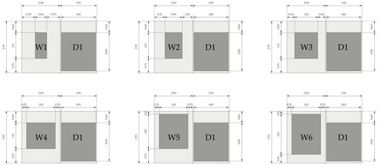
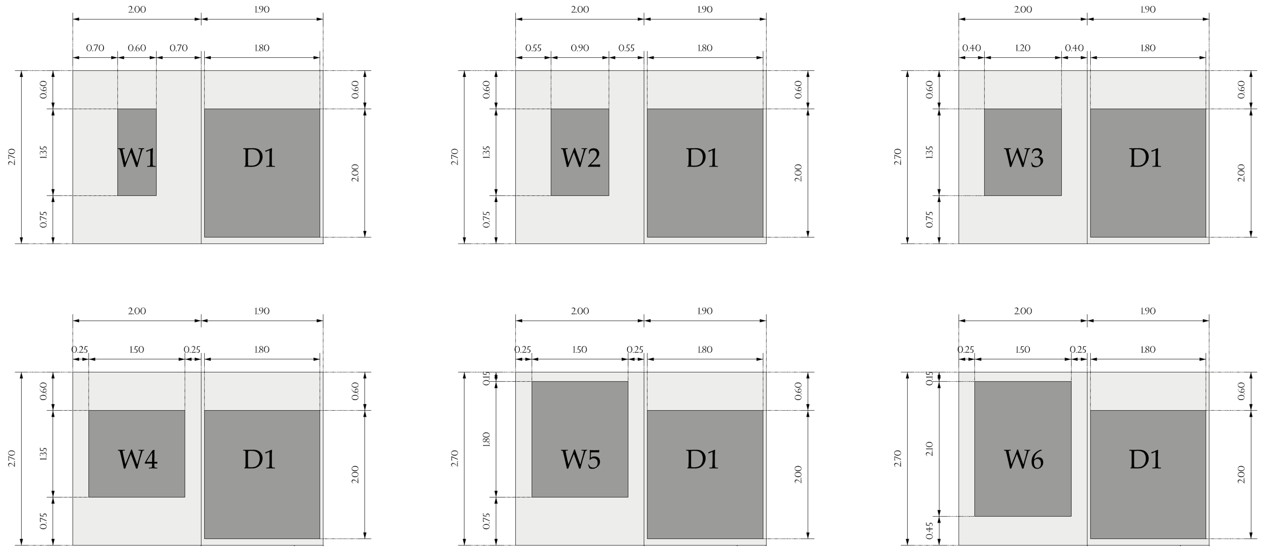
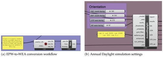
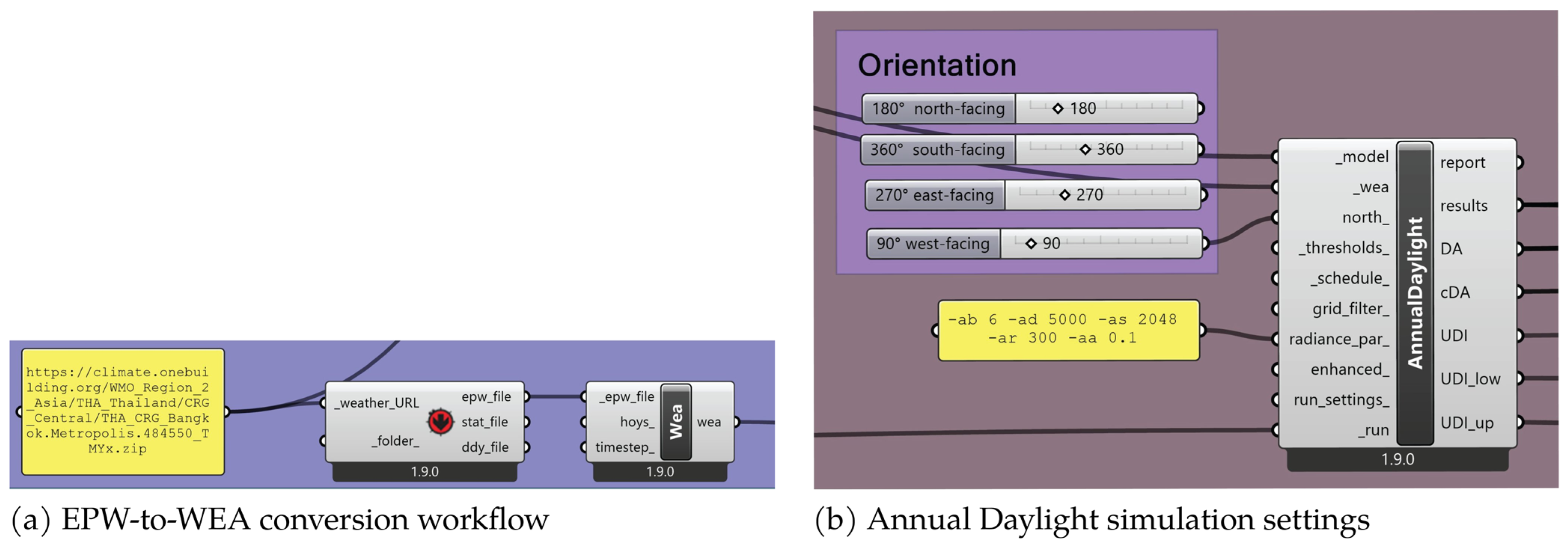
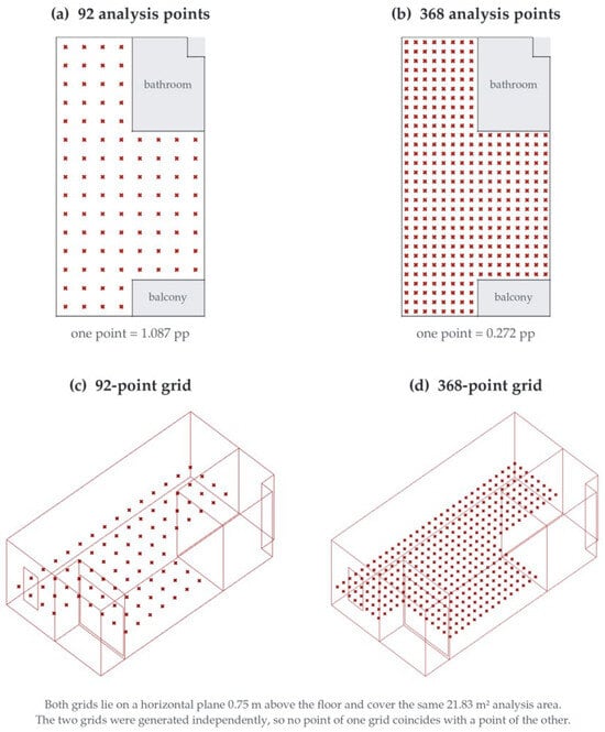
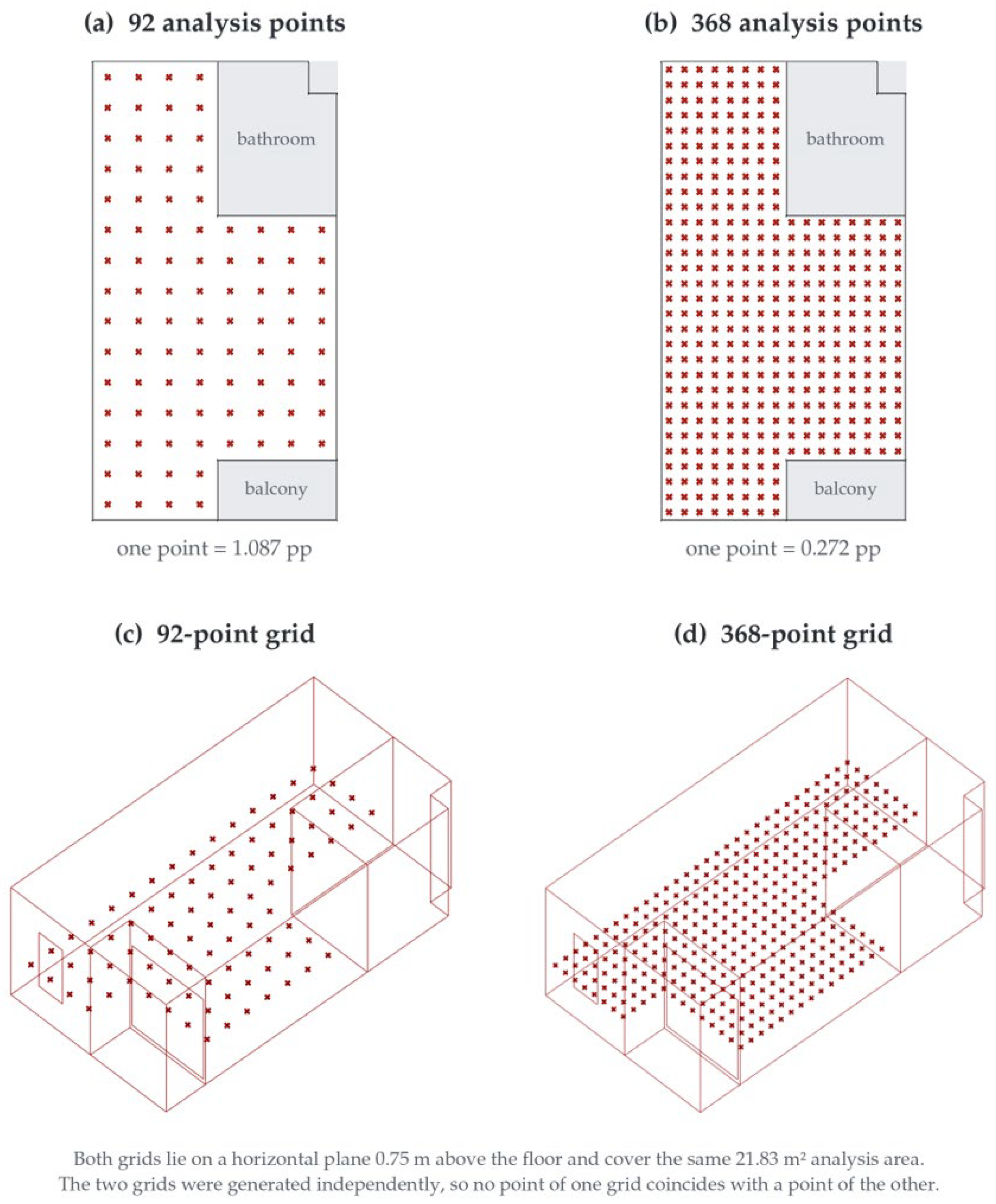
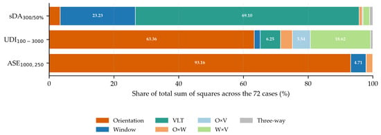
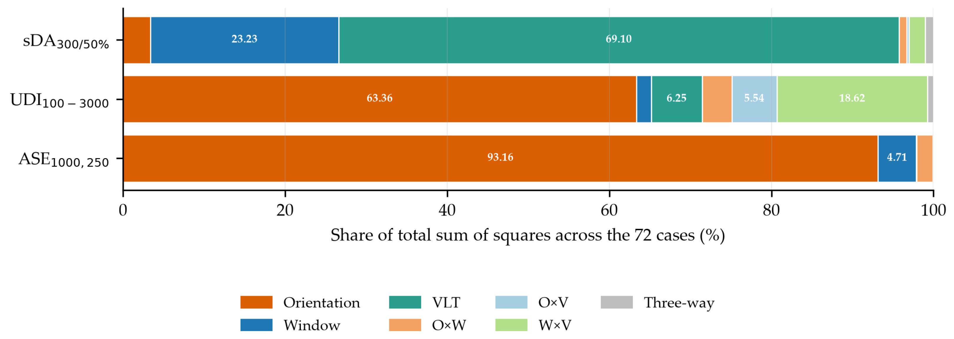
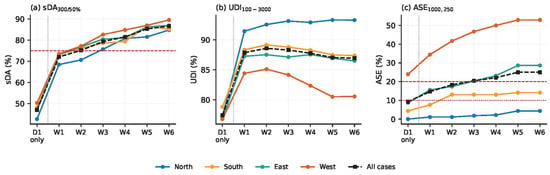
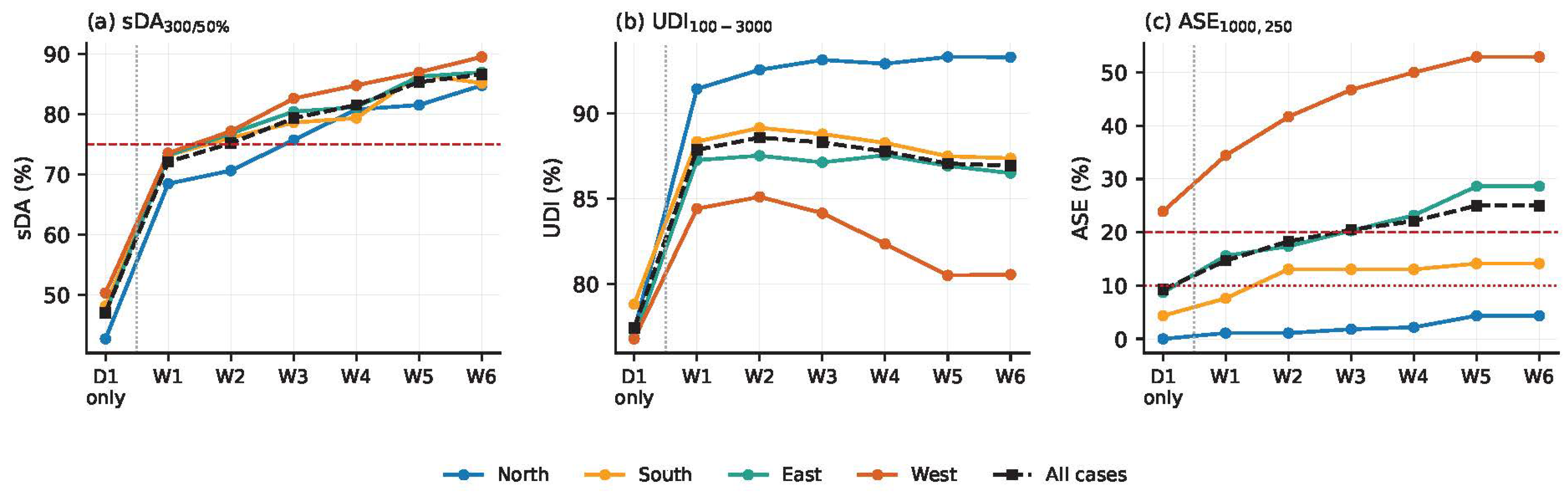
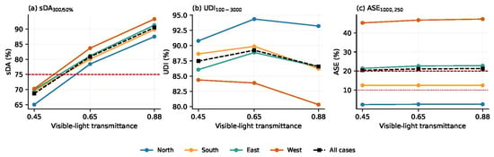
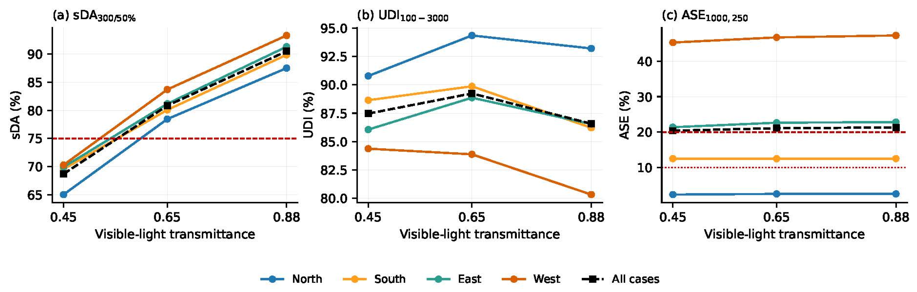
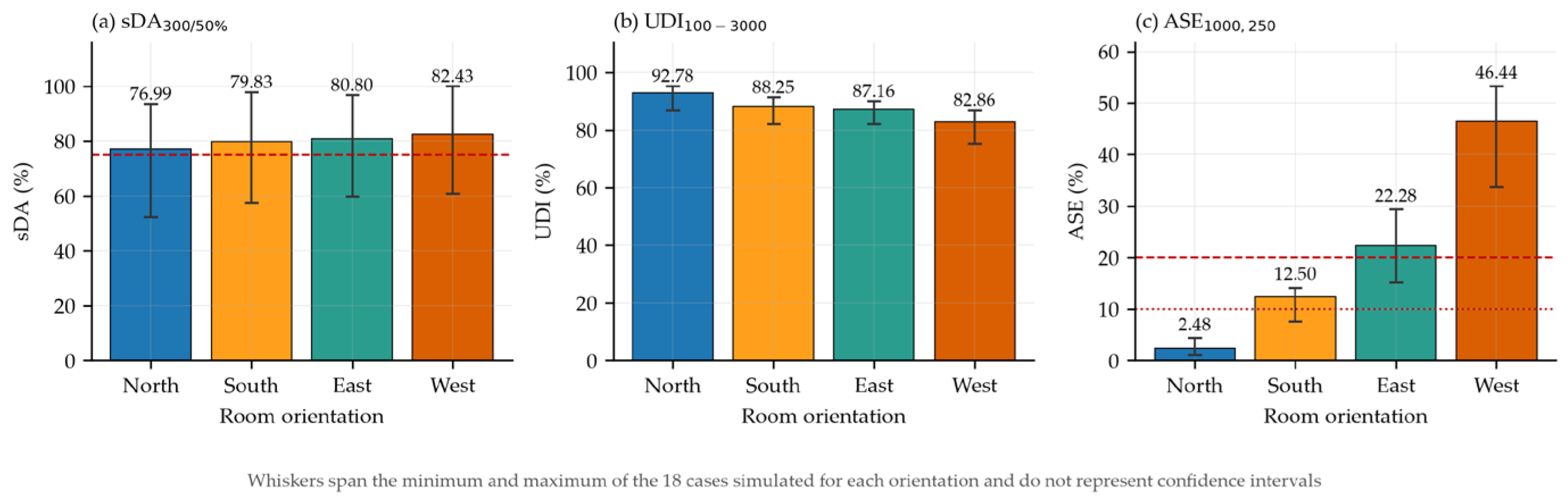
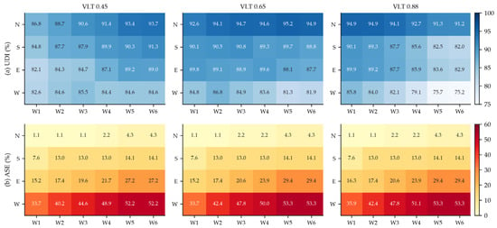
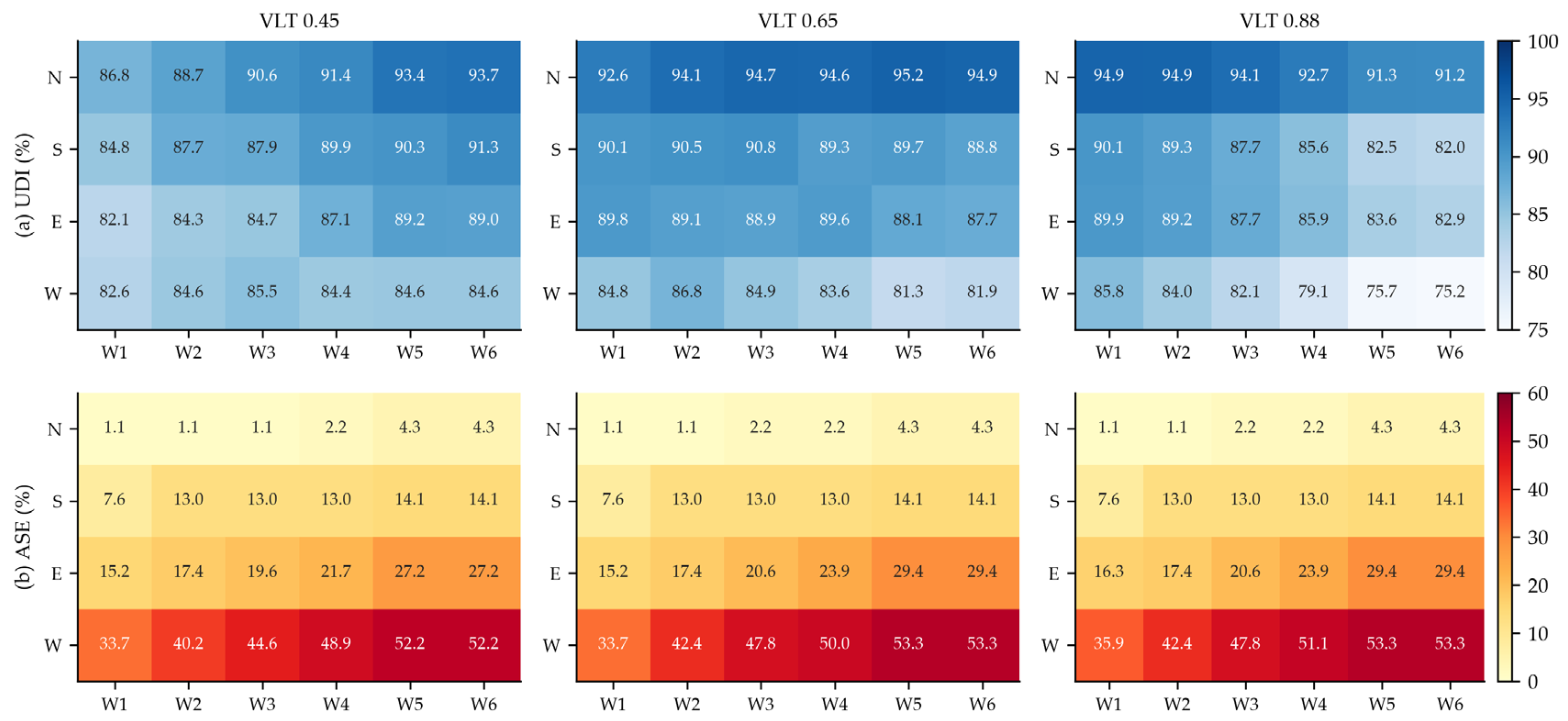
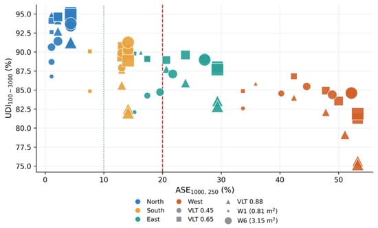
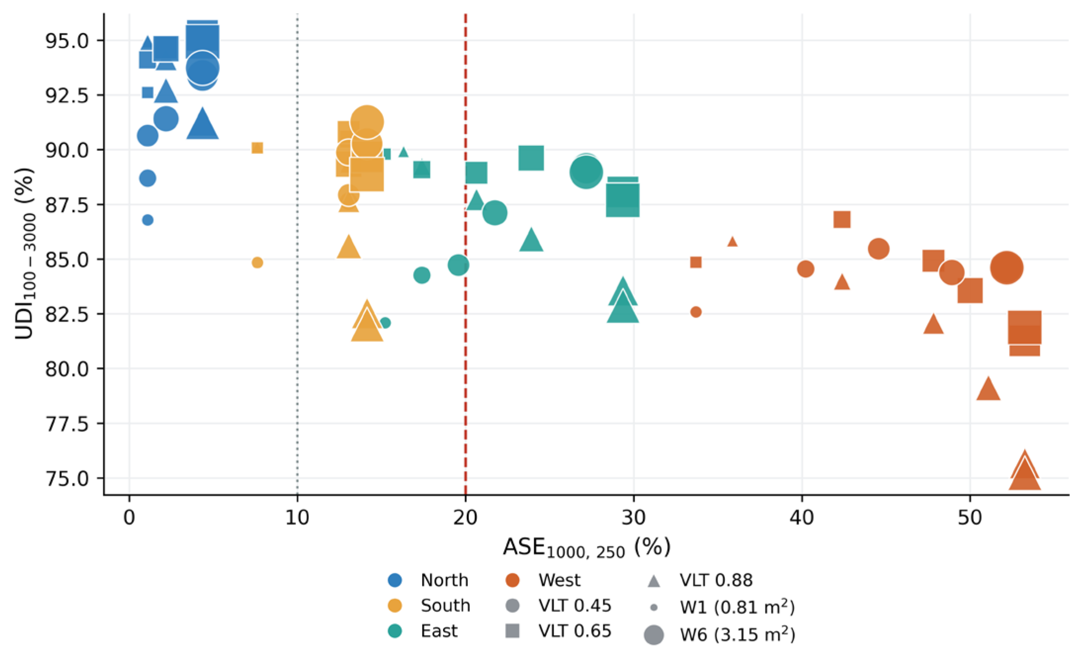
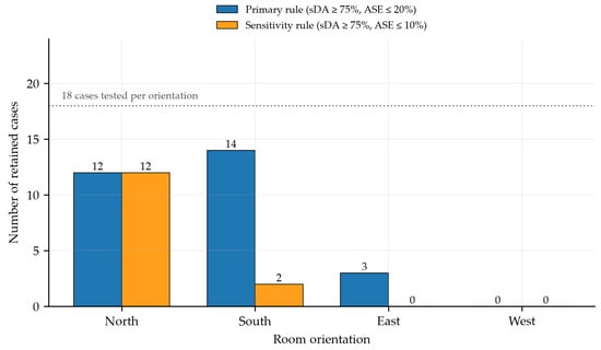
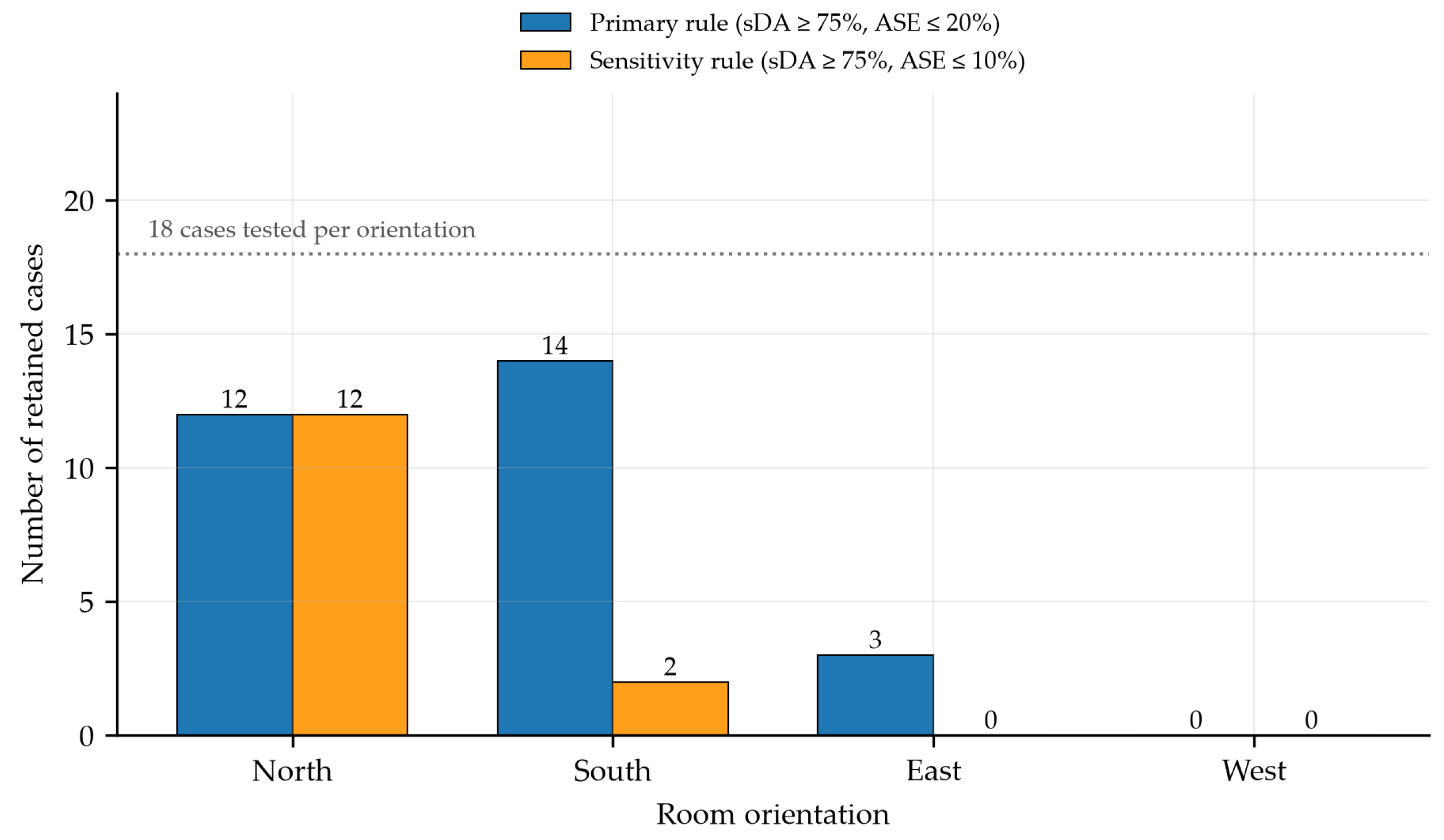
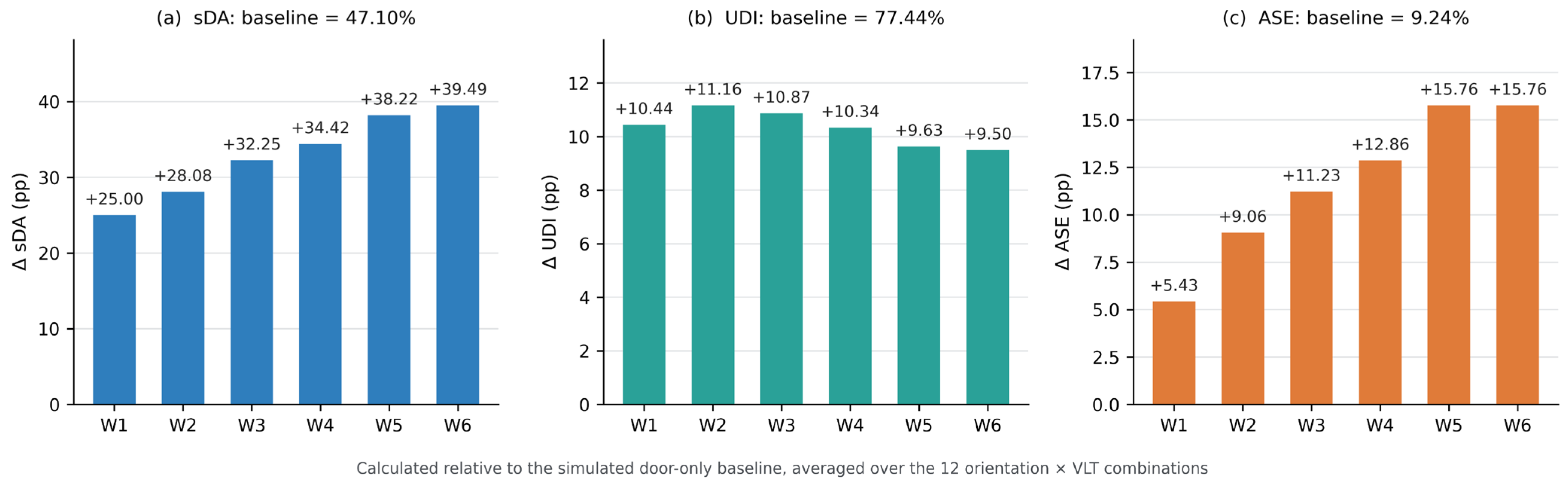
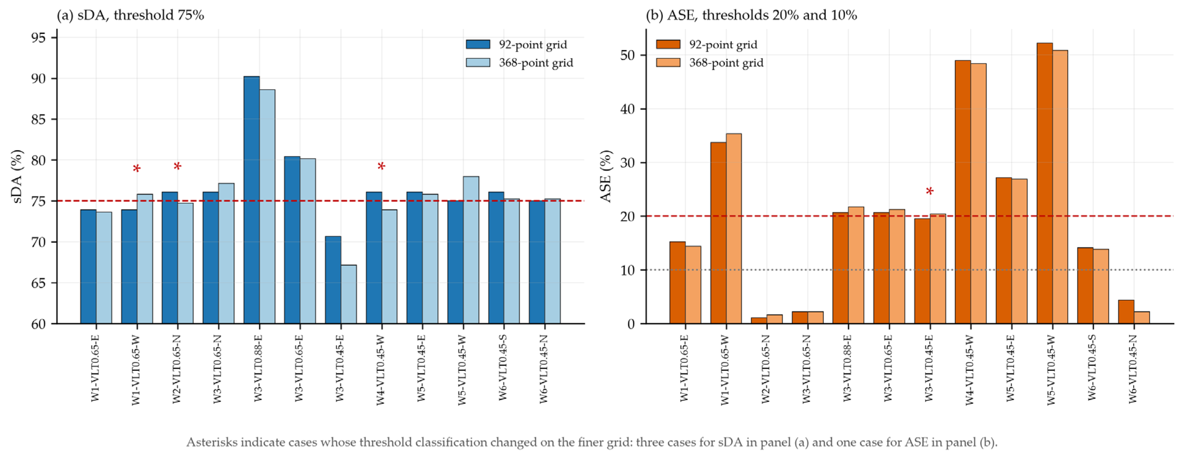

Disclaimer/Publisher’s Note: The statements, opinions and data contained in all publications are solely those of the individual author(s) and contributor(s) and not of MDPI and/or the editor(s). MDPI and/or the editor(s) disclaim responsibility for any injury to people or property resulting from any ideas, methods, instructions or products referred to in the content. |
© 2026 by the authors. Licensee MDPI, Basel, Switzerland. This article is an open access article distributed under the terms and conditions of the Creative Commons Attribution (CC BY) license.