


Abstract
The linkage between construction output prices and international commodity markets has become increasingly pronounced, yet evidence on how commodity price shocks relate to final construction output prices remains limited. Existing studies typically rely on material input cost indices, creating a tautological overlap between commodity prices and the dependent variable, while assuming symmetric linear relationships that overlook directional heterogeneity. This study employs the U.S. Producer Price Index (PPI) for new nonresidential building construction, which reflects contractors’ bid prices, as the dependent variable. Using World Bank commodity price data and quarterly observations for 2010–2025, a nonlinear autoregressive distributed lag (NARDL) model examines the asymmetric pass-through of international iron ore, crude oil, and non-ferrous metal prices to U.S. construction output prices. The results reveal a stable long-run cointegration relationship and ratchet-type asymmetry in non-ferrous metal price adjustment: a 1% increase in non-ferrous metal prices is associated with an approximately 0.36% increase in construction output prices in the long run, whereas the association of price declines is statistically insignificant. No cointegration is identified under the conventional symmetric specification. However, this asymmetry is sensitive to the inclusion of macroeconomic controls. Scenario projections indicate that a 10% rise in non-ferrous metal prices corresponds to an approximately 3.7% increase in construction output prices within three years, providing illustrative benchmarks for contingency planning, procurement, and hedging.
1. Introduction
The construction industry is a cornerstone of the national economy and depends heavily on upstream commodities such as steel, non-ferrous metals, and energy. Material costs typically account for a substantial share of total project costs, making construction prices highly sensitive to fluctuations in commodity markets. A systematic review by Musarat et al. [1] identified changes in material prices, labor wages, and equipment rental rates as major drivers of budget inaccuracies and cost overruns, while noting that price uncertainty is often inadequately incorporated into project cost analyses. Their empirical evidence further demonstrated that fluctuations in the macroeconomic price environment are systematically reflected in construction material markets [2]. As commodity pricing has become increasingly integrated into global markets, international commodity price fluctuations have emerged as an important exogenous source of cost uncertainty for the construction industry. Quantifying how, and how asymmetrically, such shocks are linked to final construction output prices (contractors’ bid prices) is therefore essential for engineering cost estimation, contingency setting, and procurement risk management.
Between 2010 and 2025, global commodity markets experienced several distinct price cycles, including the post-2011 correction, the supply-driven downturn during 2014–2016, the unprecedented surge associated with the COVID-19 pandemic and geopolitical conflicts during 2020–2022, and the subsequent decline and divergence since 2023. Such fluctuations have substantial implications for construction projects. Based on 258 large-scale infrastructure projects, Flyvbjerg et al. [3] showed that cost underestimation and overruns are persistent and widespread. Macroeconomic studies have likewise established that commodity price shocks show significant associations with the real economy. Hamilton [4] demonstrated that sharp increases in crude oil prices preceded most post-war U.S. recessions, while Kilian [5] further showed that the economic consequences depend on the underlying sources of oil price shocks. However, an important empirical observation remains insufficiently explained: despite the sharp decline in international commodity prices during 2022–2023, construction output prices in the United States and other major economies remained elevated or continued to rise rather than falling accordingly. This pattern suggests that commodity price transmission to construction output prices may be inherently asymmetric, implying that price increases and price decreases are not transmitted in the same manner. Existing studies have several limitations in addressing this issue. First, most studies employ construction input cost indices, such as the widely used ENR Construction Cost Index, to examine commodity price transmission. Because these indices are themselves constructed from material prices (e.g., steel and cement) and labor costs using fixed weights [6], regressing commodity prices on such indices introduces a tautological overlap between explanatory and dependent variables. Consequently, these measures cannot reveal whether, or to what extent, commodity price shocks are ultimately reflected in contractors’ bid prices, which more directly reflect final construction output prices. Second, previous studies predominantly rely on symmetric linear models that implicitly assume identical transmission mechanisms for price increases and decreases. Extensive empirical evidence across industries, however, has shown that price transmission is often systematically asymmetric [7]. Imposing symmetry may therefore bias parameter estimates and even obscure the existence of long-run equilibrium relationships. Third, the analysis of non-stationary price series requires econometric approaches that simultaneously address spurious regression and potential asymmetry. Nevertheless, nonlinear dynamic models capable of accommodating both non-stationarity and asymmetric adjustment remain rarely applied in construction economics.
To address these gaps, this study examines whether international commodity price shocks are asymmetrically linked to U.S. construction output prices—specifically, whether upward shocks are reflected in contractors’ bid prices more strongly than downward shocks. To identify this potential asymmetric pass-through, we use the Producer Price Index (PPI) for New Nonresidential Building Construction, which captures contractors’ bid prices rather than input costs. Combining World Bank commodity price data with quarterly observations from 2010–2025, we apply a nonlinear autoregressive distributed lag (NARDL) model [8] that distinguishes between positive and negative price changes. This study differs from the construction cost forecasting literature [6]. While those studies aim to improve predictive accuracy using leading indicators, our objective is to identify directional asymmetry in price pass-through—that is, whether commodity price increases and decreases are reflected differently in final bid prices. We therefore focus on transmission elasticities and dynamic multipliers rather than out-of-sample forecasting accuracy.
This study makes three contributions. First, it provides empirical evidence of asymmetric pass-through from international commodity price shocks to U.S. construction output prices: positive non-ferrous metal price shocks are significantly associated with higher construction bid prices, whereas negative shocks show no statistically identifiable pass-through. This directional heterogeneity is overlooked by conventional symmetric models. Second, by using a construction output price index rather than an input cost index, we examine the transmission link between international commodity markets and contractors’ bid prices while avoiding the tautological overlap inherent in input-based measures. Third, we show that the long-run equilibrium relationship cannot be identified under conventional symmetric specifications, highlighting that asymmetric modeling is important for understanding commodity price transmission to construction output prices. The estimated dynamic multipliers are translated into scenario-based projections, indicating that a 10% increase in non-ferrous metal prices corresponds to an approximately 3.7% increase in construction output prices within three years, whereas an equivalent price decline yields no identifiable cost reduction. These illustrative benchmarks inform contingency planning, procurement timing, and hedging decisions, and suggest that cost control strategies should focus primarily on periods of rising commodity prices. The remainder of this paper is organized as follows. Section 2 reviews the relevant literature. Section 3 presents the theoretical framework and research hypotheses. Section 4 describes the data and methodology. Section 5 reports the empirical results. Section 6 discusses the findings and translates them into scenario-based cost projections, and Section 7 concludes the paper and presents policy implications.
2. Literature Review
2.1. Drivers and Macroeconomic Effects of International Commodity Price Fluctuations
The macroeconomic consequences of commodity price shocks have long been a central topic in energy and resource economics. Hamilton [4] demonstrated, using postwar U.S. data, that increases in crude oil prices consistently preceded economic recessions, laying the foundation for research on the real economic effects of oil price shocks. Kilian [5] substantially advanced this literature by developing a structural vector autoregression (SVAR) model that decomposed oil price fluctuations into crude oil supply shocks, global aggregate demand shocks, and oil market-specific demand shocks, showing that each type of shock generates distinct macroeconomic outcomes. From an institutional perspective, Tang and Xiong [9] documented a significant increase in price comovement among commodities included in commodity indices, providing evidence for the financialization of commodity markets. Cheng and Xiong [10] further reviewed how financialization has reshaped the risk-sharing and price discovery functions of commodity futures markets. Focusing on the sharp oil price collapse during 2014–2016, Baffes et al. [11] attributed the downturn to a combination of supply, demand, and policy factors, while emphasizing the dominant role of supply-side shocks. Collectively, these studies indicate that international commodity price fluctuations are jointly driven by fundamental and financial factors and possess substantial potential for cross-market transmission.
2.2. Commodity Price Fluctuations and Construction Output Prices
The relationship between commodity prices and construction output prices has received sustained attention in construction economics. Akintoye et al. [12] were among the first to identify macroeconomic leading indicators of construction contract prices. Using the U.S. ENR Construction Cost Index, Ashuri and Lu [6] examined its statistical properties through univariate time-series analysis, while Ashuri et al. [13] employed cointegration and Granger causality tests to identify the Consumer Price Index (CPI), crude oil prices, and the Producer Price Index (PPI) as significant leading indicators. Shahandashti and Ashuri [14] further demonstrated that multivariate forecasting models outperform univariate benchmarks, whereas Hwang [15] proposed a time-series framework for forecasting construction cost indices. Subsequent studies extended this line of research to specific construction sectors. Shahandashti and Ashuri [16] adopted crude oil prices and average hourly earnings in the construction industry as leading indicators to forecast the U.S. National Highway Construction Cost Index using a vector error correction model (VECM), identifying two quarters as the optimal lag length. Faghih and Kashani [17] applied a similar framework to forecast U.S. asphalt, steel, and cement prices based on macroeconomic indicators. Joukar and Nahmens [18] modeled the conditional volatility of construction cost indices using a generalized autoregressive conditional heteroskedasticity (GARCH) approach, while Shiha and El-adaway [19] incorporated macroeconomic indicators from major trading partners to improve forecasts of U.S. construction material prices. Overall, the existing literature consistently demonstrates the predictive power of commodity prices for construction cost indices and confirms the suitability of cointegration and error correction frameworks for modeling such relationships. Nevertheless, most studies rely on input-based composite cost indices that inherently include material price components as dependent variables. Their primary objective is to improve forecasting accuracy rather than to examine the transmission mechanism from commodity prices to final construction output prices. Furthermore, all existing studies adopt symmetric linear specifications, implicitly assuming that commodity price increases and decreases are transmitted with identical intensity.
Recent studies have increasingly adopted data-driven approaches for construction price forecasting. Liu et al. [20] reviewed machine-learning-based methods for construction materials price prediction, highlighting the growing application of artificial intelligence techniques in this field. Recent empirical studies have demonstrated the potential of advanced deep-learning architectures, including VMD–LSTM–GRU and VMD–GRU frameworks with attention mechanisms, for improving construction cost index forecasting accuracy [21,22]. Ma et al. [23] further summarized the development of price forecasting models in the construction industry. However, these studies mainly focus on predictive performance rather than the asymmetric transmission mechanism through which commodity price fluctuations are reflected in construction output prices. From a methodological perspective, the NARDL framework is suitable for the present study because it enables asymmetric decomposition of explanatory variables and accommodates variables with mixed integration orders [8]. Recent evidence further confirms that copper futures prices exhibit chaotic, deterministic nonlinear dynamics rather than purely stochastic behavior, with efficiency differences between Chinese and international markets [24].
2.3. Construction Cost Risk and Cost Overruns
Another stream of research focuses on the consequences and management of construction cost risk. Based on cross-national evidence from 258 large-scale infrastructure projects, Flyvbjerg et al. [3] demonstrated that project costs are systematically underestimated and that this bias has persisted for decades. From the perspective of inflation and input price fluctuations, Musarat et al. [1] identified changes in construction material prices, labor wages, and equipment rental rates as major contributors to budget inaccuracies and recommended incorporating price fluctuations into dynamic project budgeting. Their empirical study further confirmed a significant relationship between inflation and the prices of major construction materials [2]. Collectively, these studies highlight the importance of understanding the transmission of upstream price shocks for effective construction cost management. However, they provide limited quantitative evidence regarding the magnitude and directional characteristics of price transmission.
2.4. Asymmetric Price Transmission
The directional dependence of price transmission was first systematically documented in retail energy markets. Bacon [25] found that retail gasoline prices in the United Kingdom responded more rapidly to cost increases than to cost decreases, a phenomenon commonly described as the ”rockets and feathers” effect. Using U.S. data, Borenstein et al. [26] confirmed that retail gasoline prices adjust significantly faster following increases in crude oil prices than following decreases, attributing this asymmetry to oligopolistic coordination and consumer search costs. Extending the analysis to more than 200 product markets, Peltzman [7] showed that approximately two-thirds of the markets exhibited asymmetric transmission, with output prices responding more rapidly to input cost increases than to decreases. Importantly, this pattern could not be fully explained by market concentration, suggesting that asymmetric price transmission is a pervasive feature of price formation rather than an anomaly confined to specific markets. Meyer and von Cramon-Taubadel [27] subsequently provided a comprehensive review of both the theoretical explanations—including market power, menu costs, inventory behavior, and policy intervention—and the econometric approaches used to analyze asymmetric price transmission. Related macroeconomic evidence likewise indicates that responses to energy price increases and decreases may differ [28]. Methodologically, Shin, Yu and Greenwood-Nimmo [8] proposed the nonlinear autoregressive distributed lag (NARDL) model, which decomposes explanatory variables into positive and negative partial sums, allowing long-run asymmetric cointegration and short-run asymmetric dynamics to be estimated simultaneously within a single-equation framework. The NARDL model accommodates a mixture of I(0) and I(1) variables and performs well with relatively small samples, making it one of the most widely adopted approaches for investigating asymmetric price transmission. Nevertheless, empirical applications have largely focused on energy, agricultural, and consumer goods markets. Evidence on asymmetric pricing behavior in construction bidding markets, particularly regarding contractors’ responses to increases and decreases in input costs, remains scarce, especially from the perspective of construction output prices.
2.5. Literature Summary
The existing literature provides a solid foundation for the present study in three respects. First, studies in macroeconomics have established the real economic effects of commodity price shocks and highlighted the amplifying role of commodity market financialization. Second, research in construction economics has demonstrated the leading role of commodity prices in explaining construction cost indices and confirmed the applicability of cointegration and error correction models for analyzing such relationships. Third, evidence from multiple industries suggests that asymmetric price transmission is a widespread phenomenon, while the NARDL framework offers a well-established econometric approach for identifying such asymmetries. Despite these advances, several important gaps remain. First, most previous studies employ input-based composite cost indices as dependent variables, providing limited evidence on whether international commodity price shocks are ultimately reflected in contractors’ bid prices. Second, construction economics studies have almost exclusively relied on symmetric model specifications, leaving the potential differences between upward and downward price transmission unexplored. If the true transmission process is asymmetric, imposing symmetry may even obscure the existence of a long-run equilibrium relationship. Third, the literature on asymmetric price transmission has rarely examined construction bidding markets. To address these gaps, this study adopts a construction output price perspective and applies the NARDL framework to provide direct empirical evidence on the asymmetric cross-market transmission of international commodity prices to final construction output prices.
3. Theoretical Mechanism and Hypotheses
International commodity prices are reflected in construction output prices primarily through two mechanisms: input costs and contractors’ pricing behavior. The former determines whether commodity price shocks are passed on to contractors’ production costs, whereas the latter determines whether and to what extent cost changes are incorporated into contractors’ bid prices. Accordingly, this section first examines the major transmission channels through which different categories of commodities affect construction output prices and then discusses how bidding behavior may generate asymmetric price transmission. These theoretical arguments provide the basis for the research hypotheses developed in Section 3.2.
3.1. Transmission Mechanisms
3.1.1. Direct Material Channel: Metal Commodities
Metal products constitute one of the most important direct inputs in construction projects, although different categories of metals exhibit distinct transmission mechanisms. Non-ferrous metals, such as copper and aluminum, are widely used in electrical systems, mechanical installations, HVAC pipelines, and building envelope systems, particularly in office, industrial, and warehouse buildings. Because internationally traded non-ferrous metals are generally priced according to benchmark prices established in global markets, such as the London Metal Exchange (LME), their procurement costs are closely linked to international market prices. Consequently, changes in international non-ferrous metal prices can be transmitted relatively directly to contractors’ material costs through a comparatively short supply chain with limited intermediate adjustments. In contrast, ferrous metal prices are transmitted through a more complex industrial chain linking iron ore, steel production, and structural construction. International iron ore prices first affect steel production costs before influencing the procurement prices of structural steel used in construction projects. In the United States, however, this transmission pathway has been substantially affected by trade policy. The weaker long-run association between international iron ore prices and U.S. construction output prices may partly reflect institutional factors affecting the domestic steel supply chain. The Section 232 tariffs introduced in 2018 altered the cost structure of steel-related industries; Flaaen and Pierce [29] show that these tariffs increased producer prices through higher input costs, suggesting that trade-policy interventions can modify conventional commodity-price transmission channels. This interpretation should be treated cautiously, however, as the estimated coefficient may also reflect proxy limitations. As a result, international iron ore price shocks may be substantially diluted before reaching the U.S. construction market. Therefore, although steel accounts for a considerable share of construction material costs, the association between international iron ore prices and U.S. construction output prices is not necessarily stronger than that of non-ferrous metals.
3.1.2. Energy Channel: Crude Oil
Crude oil prices are linked to construction output prices through three principal channels. First, they directly affect fuel expenditures for construction machinery and equipment. Second, they alter the production costs of petroleum-based construction materials, including asphalt, waterproofing membranes, and plastic pipes. Third, fluctuations in fuel prices influence transportation costs for construction materials and equipment. Compared with metal commodities, energy price transmission involves a longer and more complex supply chain, encompassing petroleum refining, logistics, material manufacturing, and distribution. Along this transmission process, price signals may be partially absorbed by profit margin adjustments, inventory management, and long-term supply contracts, thereby reducing the magnitude of the shock and delaying its transmission. Shahandashti and Ashuri [16] have shown that crude oil prices typically lead highway construction output prices by approximately two quarters, which is consistent with the relatively long transmission process associated with energy prices. Moreover, fuel and transportation costs account for only a modest proportion of total construction output prices, allowing contractors to absorb part of the cost increase through profit margin adjustments rather than fully passing it on to bid prices. Consequently, the long-run impact of crude oil prices on construction output prices is expected to be weaker than their direct effect on construction input costs.
3.1.3. Asymmetric Pricing Channel: Bidding Behavior and Price Stickiness
Whether changes in input costs are systematically linked to construction output prices ultimately depends on contractors’ bidding behavior, which typically differs between periods of rising and falling costs. When input costs increase persistently, contractors have strong incentives to pass these additional costs on to clients. Failure to incorporate expected cost increases into bid prices may substantially compress profit margins or even result in financial losses after contract award. Consequently, contractors tend to adjust bid prices upward promptly and may further mitigate future price uncertainty through contractual price adjustment clauses. By contrast, declining input costs do not necessarily lead to lower bid prices. Existing contracts often lock in agreed prices, preventing immediate adjustments to ongoing projects. In addition, construction bidding is inherently strategic. When competing contractors maintain existing bid levels, unilateral price reductions may erode profit margins without substantially improving the probability of winning contracts. This mechanism is conceptually similar to the oligopolistic coordination and consumer search cost arguments identified by Borenstein et al. [26] in retail energy markets. Furthermore, menu costs, information acquisition costs, and delays in owner–contractor negotiations all reduce the speed at which output price reductions are reflected in bid prices [30]. These factors jointly imply that contractors respond more rapidly to rising costs than to falling costs, giving rise to the well-known “rockets and feathers” pattern described by Bacon [25]. Cross-industry evidence further suggests that asymmetric price transmission is a common feature of the relationship between input and output prices [7]. Given the characteristics of construction markets—including long-term contracts, competitive bidding, and relatively infrequent transactions—price transmission is theoretically expected to exhibit even stronger asymmetry than in many other industries.
3.2. Research Hypotheses
Based on the theoretical mechanisms discussed above, this study proposes the following hypotheses.
Hypothesis 1 (H1).
International commodity prices and U.S. construction output prices exhibit a stable long-run cointegration relationship. International commodity prices are continuously linked to construction output prices through material and energy inputs. Consequently, construction output prices are expected to maintain a long-run equilibrium relationship with international commodity prices. When short-run deviations from equilibrium occur, the error correction mechanism is expected to restore the system gradually to its long-run equilibrium.
Hypothesis 2 (H2).
Increases in international commodity prices are significantly associated with higher U.S. construction output prices, with direct material channels exhibiting stronger long-run linkages than indirect channels. Among the commodities considered, non-ferrous metals are expected to have the strongest long-run transmission effect because of their relatively short transmission chain and close linkage to international benchmark prices. By contrast, the transmission of iron ore prices may be weakened by industrial chain adjustments and U.S. trade policies, whereas the long-run association of crude oil prices is expected to be further attenuated by multi-stage buffering mechanisms and contractors’ profit margin adjustments.
Hypothesis 3 (H3).
Because the bidding-behavior mechanisms in Section 3.1.3 operate through contractors’ pricing decisions, directional asymmetry is expected to be identifiable primarily in the most direct, least attenuated channel—non-ferrous metal prices (Section 3.1.1). Specifically, non-ferrous metal price transmission to U.S. construction output prices is hypothesized to be directionally asymmetric, with price increases generating stronger long-run effects than price decreases, producing a ratchet-type pattern in the MTL+ and MTL− coefficients. Given the weaker, more attenuated transmission expected for iron ore and crude oil (Section 3.1.1–Section 3.1.2), asymmetry is not separately hypothesized for these channels; whether they also exhibit asymmetric pass-through is treated as an open empirical question, addressed as a supplementary check in Section 5.6.
The three hypotheses are evaluated through the empirical analyses presented in Section 5. Specifically, H1 is tested using the bounds cointegration test, H2 through the estimation of long-run elasticities, and H3 using the Wald test for long-run asymmetry. It should be noted that the expected differences in transmission strength proposed in H2 constitute an empirical proposition rather than a theoretical certainty. If the long-run effects of the indirect transmission channel are statistically insignificant, the results would provide further support for the industrial chain attenuation and price buffering mechanisms discussed in Section 3.1.1 and Section 3.1.2.
4. Data and Methodology
4.1. Variables and Data Sources
Although the title refers to construction output prices for brevity, the dependent variable strictly measures contractors’ bid prices for newly constructed nonresidential buildings. The dependent variable is the U.S. Producer Price Index (PPI) for New Nonresidential Building Construction (UCC), compiled by the U.S. Bureau of Labor Statistics (BLS). This index measures contractors’ bid prices for newly constructed nonresidential buildings and therefore represents construction output prices rather than construction input costs. The use of an output price index instead of a construction cost index is central to the research design of this study. Input-based indices, such as the ENR Construction Cost Index and various construction material price indices, are mechanically constructed from commodity prices (e.g., steel and cement) and labor costs using fixed weights. Regressing commodity prices on these indices largely reproduces their construction methodology and therefore cannot determine whether commodity price shocks are ultimately reflected in contractors’ bid prices through pricing behavior. By contrast, the output price index incorporates contractors’ pricing decisions, making it possible to examine the complete transmission process and providing the necessary basis for identifying the asymmetric pricing mechanism discussed in Section 3. The UCC series has been published monthly since June 2009 and is publicly available through the Federal Reserve Economic Data (FRED) database (Series ID: WPU801).
The core explanatory variables consist of three categories of international commodity prices: the international iron ore spot price (IRN), the Brent crude oil spot price (OIL), and the non-ferrous metal price index (MTL). All commodity data were obtained from the World Bank Commodity Markets Outlook (Pink Sheet) monthly database. Two methodological considerations motivated the selection of these variables. First, iron ore prices were used instead of finished steel prices because the World Bank database does not provide a consistent international steel price series, whereas iron ore serves as the global benchmark for steel production. This choice ensures that all explanatory variables are measured using internationally comparable market prices and avoids contamination from domestic steel prices that are directly affected by country-specific trade policies. Whether iron ore prices are effectively reflected in U.S. construction output prices remains an empirical question addressed through Hypothesis 2. Second, the non-ferrous metal variable is represented by the Base Metals (excluding iron ore) index. The index covers aluminum, copper, lead, nickel, tin, and zinc—the primary non-ferrous metals used in nonresidential construction (electrical, HVAC, roofing, and piping; Section 3.1.1). Although not weighted by sectoral consumption shares, it is highly correlated with the U.S. BLS Producer Price Index for non-ferrous metal products (r = 0.94, 2010–2025), indicating adequate representativeness for this study.
All monthly series were converted to quarterly frequency by selecting end-of-quarter observations rather than quarterly averages. This approach was adopted for econometric reasons. Averaging overlapping monthly observations mechanically introduces moving-average serial correlation into quarterly data [31], potentially affecting residual diagnostics in dynamic models. In contrast, end-of-quarter sampling preserves the point-observation properties of the original series and avoids this artificial source of serial correlation. To ensure that the baseline findings are not driven by the temporal aggregation method, the preferred NARDL model was re-estimated using quarterly average prices and monthly frequency data as robustness checks (Section 5.6 and Appendix A Table A4). All variables were transformed into natural logarithms so that the estimated coefficients can be interpreted as elasticities.
The sample covers the period from the first quarter of 2010 to the fourth quarter of 2025, yielding 64 quarterly observations. The sample begins in 2010, the year when the global iron ore market completed its transition from annual benchmark contracts to index-linked spot pricing. Wilson [32] documents this restructuring of the Asia-Pacific iron ore market, while Wårell [33] provides direct evidence on how the pricing regime change affected iron ore price dynamics. Restricting the sample to the post-reform period ensures a consistent market-based pricing regime throughout the analysis and avoids structural breaks associated with changes in the pricing mechanism. The definitions and sources of all variables are summarized in Table 1.
Table 1.
Definitions and data sources of variables.
4.2. NARDL Model Specification
The theoretical analysis in Section 3 suggests that contractors’ bidding behavior differs between periods of rising and falling input costs, giving rise to direction-dependent price transmission that cannot be adequately captured by conventional symmetric linear models. To account for this feature, this study employs the nonlinear autoregressive distributed lag (NARDL) model proposed by Shin et al. [8].
Based on the transmission mechanisms discussed in Section 3 and the characteristics of the commodity markets, the asymmetric decomposition is applied to the non-ferrous metal price index (MTL), which is expected to exhibit the shortest transmission chain and the strongest transmission effect. This choice is consistent with H3 as formulated in Section 3.2, which hypothesizes directional asymmetry specifically for the non-ferrous metal channel; the supplementary decomposition of iron ore and crude oil prices reported in Section 5.6 serves as an exploratory robustness check on this restriction rather than a formal test of H3. Specifically, changes in lnMTL are decomposed into cumulative positive and negative partial sums:
where and denote the cumulative historical increases and decreases in metal prices, respectively. The NARDL model in error correction form is specified as follows:
where ρ is the error correction coefficient, θ represents the levels coefficients, and Dt denotes the vector of outlier impulse dummy variables. The long-run transmission elasticities are given by the ratio of the levels coefficients (βk = −θk/ρ), with standard errors calculated via the delta method. Long-run asymmetry is evaluated through a Wald test, where the null hypothesis assumes symmetric transmission elasticities (θ3+ = θ3−). To test for cointegration, a bounds test is implemented by constructing an F-statistic for the joint null hypothesis that all levels coefficients are equal to zero. Comparing this statistic against the critical value bounds under Case III (unrestricted intercept and no trend) with k = 4, an F-value above the upper bound leads to the rejection of the ‘no level relationship’ null hypothesis. Benefiting from its capability to accommodate a mixture of I(0) and I(1) variables (conditioned on the absence of I(2) series, thereby requiring prior unit root testing), the NARDL framework simultaneously captures long-run equilibria and short-run dynamics within a unified single equation. Furthermore, its statistical robustness in small-to-medium samples makes it highly compatible with the empirical data structure of this study.
ΔlnUCCt = α + ρ·lnUCCt1 + θ1·lnIRNt1 + θ2·lnOILt1 + θ3+·MTLt1+ + θ3−·MTLt1 + Σiγi·ΔlnUCCt-i + Σi(φ1i·ΔlnIRNti + φ2i·ΔlnOILti + φ3i+·ΔMTLti+ + φ3i−·ΔMTLti−) + λ′Dt + εt
Threshold autoregressive (TAR) and smooth transition autoregressive (STAR) models also accommodate nonlinear dynamics, yet they differ fundamentally from NARDL in structure and purpose. TAR models require the identification of a threshold variable and threshold value to define discrete regimes, which may introduce additional specification uncertainty when the economic mechanism governing the regime transition is unclear [34]. STAR models characterize nonlinear adjustment through smooth transition functions and are mainly developed to describe regime evolution and cyclical dynamics, rather than directly estimating asymmetric long-run elasticities through positive and negative shock decompositions [35,36]. By contrast, NARDL decomposes positive and negative changes into partial sum processes within a single-equation cointegration framework, enabling the simultaneous estimation of long-run equilibrium relationships and short-run asymmetric adjustments without requiring exogenous threshold selection [8]. This framework is particularly useful in the present study, where the sample size is relatively limited and additional regime-switching parameters may reduce estimation efficiency. Therefore, NARDL provides a more suitable framework for quantifying the magnitude and direction of asymmetric commodity-price transmission to construction costs.
4.3. Robustness to Macroeconomic Controls and Real Prices
To examine whether the baseline findings are affected by omitted macroeconomic factors, we extend the NARDL framework by incorporating four quarterly control variables: the consumer price index (CPI), construction wages (WAGE), the effective federal funds rate (RATE), and private nonresidential construction spending (DEMAND). CPI, WAGE, and DEMAND are transformed into logarithmic forms, whereas RATE is retained in levels. Considering the limited sample size (T = 64 quarters), the maximum lag order is restricted to two quarters, and the final specification is determined based on BIC ranking within this restricted lag space.
Table 2 presents the robustness results with respect to macroeconomic controls. The inclusion of additional macroeconomic controls substantially reduces the magnitude and statistical significance of the MTL+ coefficient—from 0.356 (p < 0.001) in the baseline to 0.076 (p = 0.296) once CPI alone is added—and the Wald test for asymmetry no longer rejects symmetry in Models 2–5. This indicates that the central asymmetric-transmission finding is not robust to the inclusion of plausible macroeconomic controls. This sensitivity is plausibly related, at least in part, to severe multicollinearity among the trending macroeconomic and commodity-price series (Appendix A Table A1 reports variance inflation factors as high as 733 for lnCPI in the fully controlled specification), though multicollinearity alone cannot be established as the sole explanation, and genuine specification sensitivity cannot be ruled out. The parsimonious model is retained as the preferred specification not because it has been confirmed robust, but because the controlled specifications cannot be estimated with adequate precision given the available sample (T = 60).
Table 2.
Robustness to Macroeconomic Controls and Real Prices.
To examine whether the baseline asymmetry reflects a purely nominal, inflation-driven pattern, Model 6 re-estimates the NARDL specification using CPI-deflated (real) values of all four variables—the dependent variable (UCC) as well as the three commodity price series (IRN, OIL, MTL)—rather than deflating the commodity side alone. In real terms, the long-run MTL+ elasticity is 0.151 (p = 0.005), substantially smaller than the nominal baseline estimate (0.356); the Wald test continues to reject symmetry (p < 0.001), and the bounds F-statistic (7.02) confirms cointegration. The positive and statistically significant MTL+ effect, together with the rejection of symmetry, therefore remains evident after deflating both sides of the relationship, though its magnitude is substantially attenuated.
4.4. Estimation Procedure and Diagnostic Tests
All data are public (FRED WPU801; World Bank Pink Sheet). Full replication code is archived at Zenodo [https://doi.org/10.5281/zenodo.22151168], requiring only standard Python packages (Python 3.11). A software_environment.txt records package versions. The optimal lag structure was selected by exhaustive search over p ∈ {1, 2, 3} and qk ∈ {1, 2, 3} for each of the k = 4 explanatory variables, yielding 3 × 34 = 243 candidate specifications in total. BIC was preferred to AIC because it imposes a stronger penalty on model complexity in small samples. Two constraints were imposed: (i) all four variables were retained in every specification for formal testability, and (ii) qk ≥ 1 for all variables to satisfy bounds testing requirements.
Table 3 reports the top five candidate specifications. The preferred model NARDL(3; 1, 1, 1, 1) achieves the lowest BIC (−412.94), although the margin over the second-ranked model NARDL(3; 1, 1, 3, 1) is modest (ΔBIC = 0.12). The highest adjusted R2 is obtained by a more parameterized specification (NARDL(3; 2, 1, 3, 2), adj. R2 = 0.872), but the BIC-preferred model is retained for parsimony. The selected specification was NARDL(3; 1, 1, 1, 1), with an effective sample of n = 60.
Table 3.
Top five NARDL candidate specifications by BIC.
Potential influential observations were detected using a standardized residual diagnostic with a predetermined threshold of |z| > 2 in the baseline specification without dummy variables, and controlled via impulse dummy variables rather than data deletion. This procedure identified three quarters: 2016Q2, 2021Q4, and 2022Q3. Because the underlying residuals are themselves estimated from the sample, this outlier-identification procedure is necessarily data-driven and sample-dependent; nonetheless, the decision rule—a fixed threshold applied ex ante and uniformly across all specifications, rather than a post-hoc, case-by-case judgment—is objective and fully reproducible. Section 5.7 further confirms that the main results are not sensitive to this threshold choice. These three quarters correspond to the sharp commodity market reversal in early 2016 and the peak of post-pandemic supply chain disruptions during 2021–2022.
Model adequacy was evaluated using a comprehensive set of diagnostic tests, including the Breusch–Godfrey test for fourth-order serial correlation, the Breusch–Pagan test for heteroskedasticity, the Ramsey RESET test for functional form misspecification, and the Jarque–Bera test for residual normality. Parameter stability was assessed using the recursive CUSUM and CUSUMSQ tests. To guard against multicollinearity, variance inflation factors (VIFs) were computed for all short-run regressors. Influence diagnostics—Cook’s Distance, leverage (hat values), and DFBETA—were examined to detect observations exerting disproportionate influence on the estimates. Because the inclusion of outlier impulse dummies can mechanically distort conventional influence statistics (e.g., producing leverage values near unity), these diagnostics were implemented after purging the dummy-variable effects via the Frisch–Waugh–Lovell (FWL) projection, consistent with the treatment of the recursive CUSUM tests. Full results are reported in Appendix A Table A3 and Figure A1 (Appendix B). Because the impulse dummy variables remain zero during the early recursive estimation period and may lead to singularity in the initial estimation window, the stability tests were implemented using partial regressions after removing the dummy variables according to the Frisch–Waugh procedure. Robustness was examined from three perspectives. First, the model was re-estimated after removing all impulse dummy variables to assess whether the main findings depended on outlier treatment. Second, the sample period was restricted to 2015Q1–2025Q4 to evaluate the sensitivity of the results to the sample starting point. Third, a conventional symmetric ARDL model, without decomposing non-ferrous metal prices into positive and negative components, was estimated as a benchmark to directly assess the necessity of the asymmetric specification. The results of all diagnostic and robustness tests are reported in Section 5.
5. Empirical Results
This section presents the empirical findings following the estimation procedure described in Section 4.4. We first examine the temporal characteristics of the variables and their descriptive statistics (Section 5.1 and Section 5.2), followed by unit root tests (Section 5.3) and the bounds test for cointegration (Section 5.4). The long-run asymmetric transmission elasticities, short-run dynamics, and cumulative dynamic multipliers are then reported (Section 5.5). Finally, diagnostic tests and three robustness checks are presented (Section 5.6).
5.1. Temporal Dynamics and Co-Movement of the Variables
Figure 1 illustrates the evolution of the logarithmic prices of the three international commodity groups over the sample period, while Figure 2 compares the U.S. nonresidential construction output price index with international commodity prices.
Figure 1.
International commodity prices (end-of-quarter observations, 2010Q1–2025Q4).
Figure 2.
Co-movement between the U.S. construction output price index and international commodity prices.
As shown in Figure 1, international commodity prices experienced several distinct cycles during the sample period, including the prolonged correction following the 2011 peak, the sharp downturn during 2014–2016 (with both iron ore and Brent crude oil reaching sample lows around 2015–2016), the unprecedented surge during 2020–2022 driven by the combined effects of the COVID-19 pandemic and geopolitical conflicts (iron ore prices peaked in mid-2021, rising by more than 1.6 log points from the sample trough), and the subsequent correction and divergence after 2023.
Figure 2 reveals two notable patterns. First, construction output prices exhibit a clear positive co-movement with international commodity prices, with the steepest increase in the output price index occurring during the commodity price boom of 2020–2022. Second, although commodity prices declined markedly after mid-2022, construction output prices did not follow the downward trend. Instead, they remained at historically high levels and continued to increase gradually. This divergence provides preliminary evidence of a ratchet-type asymmetry, whereby cost increases are reflected in construction prices, whereas cost decreases exhibit substantial downward rigidity. The raw data therefore offer an intuitive motivation for the formal asymmetric transmission analysis conducted in the following sections.
5.2. Descriptive Statistics
Table 4 reports the descriptive statistics of the logarithmically transformed variables based on 64 quarterly observations.
Table 4.
Descriptive statistics of the logarithmic variables (2010Q1–2025Q4).
As shown in Table 4, the mean value of lnUCC is 4.829, with a standard deviation of 0.204 and a range of 0.610. Its positive skewness (0.684) indicates that the upward movement in construction output prices was concentrated in the latter part of the sample period. The three international commodity price series exhibit substantially greater volatility than the construction output price index. Among them, iron ore prices show the largest dispersion (standard deviation = 0.356; range = 1.667), followed by Brent crude oil (0.330), whereas the non-ferrous metal price index is comparatively less volatile (0.195). All three commodity price variables display negative skewness, consistent with the pronounced boom-and-bust cycles observed during the sample period. Overall, the dependent variable is considerably less volatile than the explanatory variables, suggesting that international commodity price shocks are substantially smoothed and partially absorbed before being reflected in construction output prices.
Table 5 reports the Pearson correlation matrix. All four series are positively correlated, with the strongest association between iron ore and non-ferrous metal prices (r = 0.656, p < 0.01), reflecting their common exposure to global industrial demand cycles.
Table 5.
Correlation matrix of logarithmic variables (2010Q1–2025Q4).
5.3. Unit Root Tests
Table 6 presents the results of the Augmented Dickey–Fuller (ADF) and Phillips–Perron (PP) unit root tests. The level specifications include both an intercept and a deterministic trend, whereas the first-difference specifications include only an intercept.
Table 6.
Results of the unit root tests.
As reported in Table 6, the ADF and PP tests produce fully consistent results. For all four variables, the null hypothesis of a unit root cannot be rejected at levels, with ADF statistics ranging from −1.353 to −2.545 and corresponding p-values exceeding 0.30. After first differencing, all series become stationary at the 5% significance level or better. For example, the ADF statistic for ΔlnUCC is −4.380 (p < 0.001), while the corresponding PP statistic is −2.924 (p = 0.043). Overall, all variables are integrated of order one [I(1)], and none is integrated of order two [I(2)]. The integration properties therefore satisfy the prerequisites for applying the NARDL bounds testing approach.
5.4. Cointegration Test
Table 7 reports the results of the NARDL bounds test for cointegration. Based on the BIC, the preferred specification is NARDL(3; 1, 1, 1, 1), estimated using 60 quarterly observations. The F-statistic (6.587) exceeds the 1% asymptotic upper bound of 5.06 [37] (Case III, k = 4). Given n = 60, we also report finite-sample critical values from Narayan [38]: at 5%, the I(0) and I(1) bounds are 4.20 and 5.72, both comfortably exceeded by the estimated statistic. The ECT is negative and highly significant (t = −5.005). The null of no level relationship is therefore rejected at 1%, confirming cointegration. These results provide empirical support for H1.
Table 7.
NARDL Bounds Test for Cointegration.
5.5. Long-Run Asymmetric Transmission and Short-Run Dynamics
Formal Wald tests comparing the cumulative levels coefficients—which determine long-run elasticities because the common error-correction parameter cancels out under the null—confirm that the non-ferrous metal long-run elasticity differs significantly from both iron ore (p = 0.0006) and crude oil (p = 0.0102), whereas the latter two do not differ from each other (p = 0.194). These pairwise comparisons formally establish that the stronger transmission through the non-ferrous metal channel is statistically robust, although the individually insignificant iron ore and crude oil coefficients may also reflect limited statistical power or proxy limitations, as discussed in Section 6.2.
Table 8 presents the estimated long-run transmission elasticities, which constitute the central empirical finding of this study. Among the three commodity groups, only positive changes in non-ferrous metal prices exhibit a significant long-run association with construction output prices. The estimated elasticity is 0.356 (SE = 0.082, p < 0.001), indicating that a 1% cumulative increase in non-ferrous metal prices corresponds to an approximately 0.36% long-run increase in construction output prices. By contrast, the long-run coefficient associated with price decreases is 0.043 and statistically insignificant (p = 0.665), with a 95% confidence interval of [−0.156, 0.242]. This wide interval indicates uncertainty in the precise magnitude of downward transmission rather than providing evidence for a strictly economically negligible effect (see Appendix A Table A5 for the power calculations). The result is therefore interpreted as evidence of substantially weaker downward transmission relative to upward transmission, not as proof of complete absence. The null hypothesis of symmetric transmission is strongly rejected by the Wald test (p < 0.001), providing direct statistical evidence of a ratchet-type asymmetry. Accordingly, H3 is supported in the baseline specification, although this result is sensitive to the inclusion of macroeconomic controls (Section 4.3, Table 2). In contrast, the long-run elasticities of iron ore (−0.022, p = 0.477) and crude oil (0.062, p = 0.163) are statistically insignificant. Thus, the positive long-run linkage hypothesized in H2 is supported only for the non-ferrous metal channel. These findings further indicate that the identified ratchet-type asymmetry is specific to this channel, as statistically insignificant long-run elasticities are found for iron ore and crude oil prices. While the estimated ranking of transmission strength is consistent with the theoretical expectation that direct material inputs exert stronger effects than indirect channels, the latter cannot be statistically identified. As anticipated in Section 3, this finding is consistent with the dampening effects of trade-policy distortions in the iron ore channel and the multi-stage buffering mechanisms in the oil channel. These mechanisms are discussed further in Section 6.
Table 8.
Long-run Transmission Elasticities (Delta Method Standard Errors).
Table 9 reports the short-run dynamics from the error correction model. The estimated level coefficient (ρ) is −0.107 (p < 0.001), yielding an error correction speed of 10.7% per quarter, with the expected sign and magnitude, implying that approximately 11% of any deviation from the long-run equilibrium is corrected each quarter. This corresponds to a half-life of roughly six quarters, indicating a relatively slow adjustment process consistent with long construction contract cycles and infrequent price revisions. The short-run results also reveal asymmetric transmission. Positive changes in non-ferrous metal prices show an immediate and significant association (0.056, p = 0.011), whereas negative changes remain insignificant (−0.018, p = 0.431). In addition, the first lag of the dependent variable is positive and highly significant (0.344, p < 0.001), indicating strong persistence in contractors’ bidding behavior. All three outlier dummy variables are positive and statistically significant, corresponding to the sharp commodity market reversal in early 2016 and the peak of post-pandemic supply chain disruptions during 2021–2022. The model achieves an adjusted R2 of 0.853, although this statistic should be interpreted cautiously given the presence of a lagged dependent variable and intervention dummies.
Table 9.
Error correction Model Estimates.
Figure 3 reports cumulative dynamic multipliers with 95% confidence intervals derived from a parametric Monte Carlo procedure with 1000 replications. The procedure was conducted as follows: (i) estimate the baseline NARDL by OLS to obtain the coefficient vector and its asymptotic covariance matrix; (ii) draw 1000 coefficient vectors from the multivariate normal distribution implied by these estimates; (iii) for each drawn coefficient vector, simulate the cumulative dynamic response to a unit shock in the positive and negative non-ferrous metal price components using the NARDL dynamic structure; (iv) take the 2.5th and 97.5th percentiles across the 1000 simulated paths at each horizon as the 95% confidence interval. This procedure reflects parameter estimation uncertainty, captured through the estimated covariance matrix, rather than residual-resampling uncertainty. Random seed = 42. Full code is archived with the replication materials. The left panel shows a clear ratchet pattern. The multiplier for positive price shocks reaches 0.056 in the impact quarter, increases steadily thereafter, approaches approximately 0.34 by the eighth quarter, and converges to the long-run elasticity of about 0.36 after roughly twelve quarters. In contrast, the multiplier associated with negative shocks remains close to zero throughout the adjustment period, converging to approximately 0.04, with confidence intervals encompassing zero at all horizons. The right panel plots the asymmetric dynamic multiplier difference (m+ − m−), which increases over time and converges to approximately 0.31, exactly matching the difference between the two estimated long-run elasticities tested by the Wald statistic. The lower bound of the 95% confidence interval remains above zero from the impact quarter onward, indicating statistically significant asymmetry at all horizons. These dynamic responses closely corroborate the long-run elasticity estimates and provide supporting dynamic evidence for the ratchet-type transmission mechanism.
Figure 3.
Cumulative dynamic multipliers of non-ferrous metal price changes: (a) multipliers of the positive and negative components with 95% Monte Carlo confidence intervals; (b) asymmetry (m+ − m−) with 95% Monte Carlo confidence interval.
5.6. Diagnostic Tests and Robustness Checks
The baseline model satisfies the major diagnostic criteria, and Figure 4 reports the parameter stability tests. The Breusch–Godfrey test detects no evidence of fourth-order serial correlation (p = 0.120), the Breusch–Pagan test indicates homoscedastic residuals (p = 0.687), and the Jarque–Bera test confirms residual normality (p = 0.698). The Ramsey RESET test is significant at the 5% level (p = 0.034), indicating potential functional-form misspecification. Three explanations are considered. First, extreme observations during the COVID-19 and supply-chain disruption periods introduce nonlinearities that linear specifications struggle to capture; consistent with this, the RESET statistic strengthens markedly (p < 0.001) when impulse dummies are excluded, confirming that these controls absorb abnormal-period nonlinearities. Second, parameter instability is unlikely: the Quandt–Andrews-type sup-F test yields 1.231, below the conservative 5% critical bound of 2.01. Third, while the lag structure is BIC-selected, some higher-order nonlinear dynamics—likely associated with the COVID-19 and supply-chain disruption periods—unmodeled by the linear specification with impulse dummies. While the recursive CUSUM and CUSUMSQ tests confirm parameter stability and the baseline asymmetry is robust to the outlier treatment and temporal aggregation (although not to the inclusion of macroeconomic controls; Section 4.3), readers should note that the baseline model provides a linear approximation to a potentially more complex dynamic process. Future research with longer samples may benefit from explicitly nonlinear specifications such as Markov-switching or threshold autoregressive models. Moreover, the recursive CUSUM and CUSUMSQ statistics remain entirely within the 5% confidence bands, suggesting stable parameter estimates throughout the sample period. Multicollinearity is not a concern: all VIFs for short-run regressors are below 3.9 (Appendix A Table A3, Panel A), substantially below the conventional threshold of 10. The FWL-purged influence diagnostics identify a small number of observations that exceed conventional relative warning thresholds. Using Cook’s distance >4/(n − k) = 0.0816 and leverage >2k/n = 0.3667, seven and six observations, respectively, are flagged in Appendix A Table A3. However, none exceeds the more conservative absolute thresholds of Cook’s D = 1.0 or leverage = 0.8 (maximum values: 0.243 and 0.558, respectively). The flagged observations are concentrated in the 2020Q4–2022Q3 period, which overlaps with the impulse-dummy controls used for the COVID-19 and supply-chain disruption period. These diagnostics therefore indicate some localized influence but no extreme observations under the absolute criteria. Overall, the diagnostic results support the general adequacy and stability of the baseline specification, while the significant RESET statistic signals that some nonlinear dynamics may exceed the current linear framework.
Figure 4.
Parameter stability tests: (a) recursive CUSUM; (b) CUSUM of squares. The black line denotes the CUSUM statistic; the grey line denotes the zero reference line in (a) and the expected value under the null hypothesis (t/T) in (b); dashed lines denote 5% significance bands.
Table 10 evaluates the robustness of the baseline results using three alternative specifications. First, removing all outlier dummy variables leaves the main findings unchanged. The evidence for cointegration (F = 7.54), the error correction mechanism (ECT = −0.176, p < 0.001), the long-run transmission association of positive non-ferrous metal price changes (0.412, p < 0.001), and the Wald test for asymmetry (p < 0.001) all remain significant. The omission of dummy variables primarily affects the residual diagnostics, with evidence of serial correlation and non-normality emerging, indicating that the dummy variables mainly improve model adequacy rather than drive the substantive results. Second, restricting the sample to 2015–2025 reduces the sample size to 40 observations. The bounds-test statistic declines to 3.83, falling within the inconclusive region at the 5% significance level under the PSS asymptotic bounds; at the 10% level it exceeds the asymptotic upper bound, nominally supporting cointegration. Given the small subsample (T = 40), however, this 10% conclusion should be interpreted cautiously, as finite-sample critical values such as those reported by Narayan [38] may provide a more appropriate benchmark. The Wald test continues to indicate significant asymmetry (p = 0.016); however, this subsample provides a materially different characterization of that asymmetry than the full sample: the MTL+ coefficient becomes statistically insignificant (0.105, p = 0.170), while the MTL− coefficient turns negative and becomes statistically significant at the 1% level (−0.326, p = 0.004). This sign reversal in the downward-price coefficient suggests parameter instability rather than a minor deviation, plausibly related to the reduced sample size (T = 40), the concentration of this window around the COVID-19 pandemic, and the 2018 Section 232 steel tariffs. The full-sample estimates are retained as the primary basis for inference because they span a longer period and yield materially more precise estimates; the subsample results are reported as a sensitivity check indicating that the baseline MTL− estimate should not be treated as a precisely pinned-down parameter. Third, the symmetric ARDL specification provides a direct comparison with the proposed NARDL model. Imposing equal transmission effects for price increases and decreases reduces the bounds-test statistic to 2.51, below the 10% lower critical bound, eliminating evidence of cointegration. At the same time, the error correction coefficient shrinks to nearly zero (−0.017). These results indicate that the symmetric specification fails to capture the underlying long-run relationship and highlight the importance of explicitly modeling asymmetric price transmission, consistent with the arguments of Shin et al. [8]. As a further check, the positive–negative decomposition was applied to iron ore and to crude oil in turn while holding the baseline lag structure fixed; in both cases the Wald test fails to reject symmetric transmission (p = 0.226 and p = 0.187, respectively), supporting the symmetric treatment of these two channels in the baseline specification.
Table 10.
Robustness Checks.
Robustness to temporal aggregation: To address the concern that end-of-quarter observations may introduce timing-related noise for volatile commodity prices, we re-estimated the preferred NARDL specification under two alternative temporal aggregation schemes: quarterly average prices and monthly frequency data. To ensure that any differences are attributable solely to temporal aggregation, the same asymmetric decomposition procedure, joint BIC lag-selection search (p ∈ {1, 2, 3}, q ∈ {1, 2, 3}4), sample-construction rule, and outlier-identification criterion (|standardized residual| > 2.0, identified independently for each aggregation scheme) were applied across both specifications; long-run elasticities and p-values are computed using the OLS covariance matrix and delta method, consistent with the baseline specification, with HC3 robust standard errors reported separately in Section 5.7. Table 11 reports the results.
Table 11.
Robustness to Alternative Temporal Aggregation.
Table 11 confirms that Column (1) exactly reproduces the baseline model (Table 8), providing a direct validation of the estimation procedure. Under quarterly average aggregation (Column 2), the positive MTL+ effect remains statistically significant but is attenuated relative to the end-of-quarter baseline, declining from 0.356 to 0.288 (a reduction of approximately 19%); the bounds F-statistic and the Wald test for asymmetry are, if anything, stronger under this aggregation (F = 8.97 vs. 6.59; Wald p < 0.0001 vs. 0.0001). The negative shock component remains statistically insignificant in both specifications. These results indicate that the directionally asymmetric, ratchet-type transmission is not an artifact of the choice between end-of-quarter and quarterly average observations, although the precise magnitude of the long-run MTL+ elasticity is somewhat sensitive to this choice. Full results for the monthly frequency specification are reported in Appendix A Table A4.
5.7. Outlier Threshold Sensitivity and Parameter Stability
To ensure the findings are not driven by the specific outlier rule, the NARDL model was re-estimated using alternative standardized residual thresholds of 1.5σ, 2.0σ (baseline), and 2.5σ. The long-run asymmetric elasticities remain qualitatively stable across all specifications (Table 12): MTL+ is consistently significant (0.356, 0.390, 0.365; all p < 0.001), whereas MTL− remains insignificant (0.043, 0.085, 0.042), and the Wald test rejects symmetry at all thresholds (p < 0.001). These results confirm that the detected ratchet-type asymmetry is insensitive to the outlier identification criterion.
Table 12.
Alternative Outlier Threshold Robustness.
Furthermore, a Quandt–Andrews-type sup-F test based on sequential Chow statistics, without imposing a pre-defined break date, yields a sup-F statistic of 1.231, which is below the conservative 5% critical bound of 2.01. This indicates no evidence of substantial parameter instability in the NARDL specification.
Overall, the empirical evidence strongly supports H1, confirming a stable long-run cointegrating relationship between international commodity prices and U.S. construction output prices. H2 receives partial support, as only the direct material channel represented by non-ferrous metals exhibits a significant positive long-run transmission effect, whereas the iron ore and crude oil channels remain statistically insignificant. H3 is supported in the baseline specification, with the Wald test and the alternative threshold robustness both indicating that asymmetric modeling is important for identifying the long-run equilibrium relationship, although this result is sensitive to the inclusion of macroeconomic controls (Section 4.3, Table 2).
To ensure inference is robust to heteroskedasticity, we re-estimate the baseline NARDL with Huber–White heteroskedasticity-consistent standard errors. The long-run MTL+ elasticity remains 0.356 (HC3 SE = 0.080, 95% CI = [0.199, 0.512]), and the Wald test continues to reject symmetry (p < 0.001). All other reported standard errors in Table 7,
Table 8, Table 9 and Table 10 are based on conventional OLS unless explicitly labeled otherwise. We further control for two event-specific shocks: the U.S.–China tariff episode (2018Q3–2019Q4, D_TARIFF) and the COVID-19 pandemic combined with global supply chain disruptions (2020Q1–2022Q4, D_COVID_SUPPLY). The long-run MTL+ elasticity remains stable at 0.332 (SE = 0.090, 95% CI = [0.155, 0.509]), and neither dummy is significant (D_TARIFF: p = 0.999; D_COVID_SUPPLY: p = 0.410), suggesting that the asymmetric pass-through is not driven by these episodes.
5.8. Alternative Specifications and Parameter Stability
5.8.1. Alternative Model Specifications
To assess whether the asymmetric specification adds value over linear alternatives, we compare the baseline NARDL with three specifications. First, the symmetric ARDL (Table 10, Column 4) fails to identify cointegration (F = 2.51, below the 10% lower critical bound for k = 3), providing no evidence of a long-run relationship under the symmetric specification. Second, a VAR/VECM would be heavily parameterized relative to the limited quarterly sample (T = 60): a VAR incorporating all four series (UCC, IRN, OIL, and MTL) would require a substantial number of parameters, particularly at higher lag orders such as p = 3, making reliable finite-sample inference difficult [39]. Third, an ARIMAX framework is unsuitable because the objective is mechanism identification (directional asymmetry and long-run pass-through) rather than short-term forecasting.
5.8.2. Structural Break and Pre/Post Comparison
To test for a structural break at the COVID-19 onset, we conduct a Chow-type parameter stability test at 2020Q1. Given the limited post-break sample (T = 20 after differencing and lag alignment), we examine a single theoretically motivated break rather than a multiple-break test. The F-statistic for equality of the full coefficient vector across the pre-COVID (2010Q1–2019Q4) and post-COVID (2020Q1–2025Q4) sub-samples is F(15, 30) = 1.19 (p = 0.328), not rejecting parameter stability at the 5% level. Table 13 reports the sub-period estimates: the pre-COVID and post-COVID bounds F-statistics (2.50 and 2.52, respectively) fall below the 5% lower critical bound (2.86) but above the 10% lower critical bound (2.45), placing both sub-periods in the inconclusive region at the 10% level and below the lower bound at 5%; in neither case can cointegration be conclusively established within the subperiod, and the post-COVID ECT (−0.163, SE = 0.137) is itself statistically insignificant. The point estimates of the long-run MTL+ elasticity are directionally consistent with the full-sample result (0.289 pre-COVID, 0.433 post-COVID), but given the absence of confirmed cointegration in either subperiod, these sub-period elasticities are suggestive rather than confirmatory. The Chow test indicates no statistically detectable break in the full coefficient vector, which is distinct from confirming stability at the sub-period level.
Table 13.
Pre- and post-COVID NARDL estimation results.
5.8.3. Rolling-Window Estimation
To examine parameter stability, rolling-window NARDL estimation was performed using a parsimonious specification—ARDL(1; 1,1,1,1) with a single lagged dependent-variable difference—within a 48-quarter window and one-quarter step. The simplified lag structure is necessary because the 48-quarter window yields only approximately 44 effective observations after differencing, and higher-order lags would leave insufficient degrees of freedom for reliable estimation. Consequently, the rolling-window specification differs from the full-sample BIC-selected order ARDL(3; 1,1,1,1); the rolling estimates should be interpreted as providing qualitative stability evidence rather than precise replication of the full-sample elasticities. Detailed results are reported in Appendix A Table A2 and summarized in Figure 5.
Figure 5.
Rolling-window estimates of the long-run MTL+ elasticity.
As shown in Figure 5 and detailed in Appendix A Table A2, a total of 17 rolling windows were generated, among which 15 yielded valid long-run elasticity estimates after applying the predefined error-correction stability criterion (Windows 5 and 6 were excluded). Among these 15 valid windows, the MTL+ elasticity estimates were not uniformly positive: three windows (Windows 2–4, whose 48-quarter spans extend into the 2020–2022 pandemic and supply-chain disruption period) produced negative point estimates ranging from −0.470 to −0.418, while the remaining 12 windows yielded positive estimates ranging from 0.276 to 0.474 (mean ≈ 0.385). Across all 15 valid windows, the mean point estimate is 0.221 (median 0.350). In every window without exception, however, the 95% confidence interval for this elasticity includes zero (Appendix A Table A2), so no individual window’s estimate is statistically distinguishable from zero. The point estimates therefore indicate a positive tendency over most of the rolling-window sequence, but this tendency is statistically inconclusive rather than uniformly positive across all valid windows.
6. Discussion
6.1. Ratchet Transmission: Direction-Dependent Pricing in Construction Bidding
The most important finding is the pronounced directional asymmetry in price transmission. Positive shocks in international non-ferrous metal prices are associated with U.S. construction output prices with a long-run elasticity of 0.356, whereas negative shocks show a statistically insignificant coefficient of 0.043 (p = 0.665, 95% CI [−0.156, 0.242]). The Wald test strongly rejects symmetry (p < 0.001), confirming statistically significant differences between the upward and downward transmission elasticities. This pattern is highly consistent with the three mechanisms proposed in Section 3.1.3. When input costs increase, contractors are compelled to raise bid prices to avoid profit losses, making output price pass-through largely unavoidable. By contrast, when costs decline, downward adjustment is impeded by contract price rigidity in ongoing projects, strategic pricing in new bids, and delayed recognition of lower costs by project owners, all of which slow the transmission of output price reductions [27]. The short-run estimates reported in Section 5.5 further support this interpretation: the contemporaneous association of positive metal price shocks (0.056) is immediately significant, while the first-order lag of construction prices (0.344) indicates strong price persistence. The coexistence of rapid upward adjustment and persistent price inertia is consistent with the ratchet-type asymmetry.
This finding extends the evidence on the well-known “rockets and feathers” pattern from retail energy markets [25,26,40] to construction bidding [7]. More importantly, the degree of asymmetry appears considerably stronger. Whereas previous studies generally report that price decreases are transmitted only more slowly [16], our estimates suggest that downward transmission is statistically imprecise rather than economically absent. The combination of contract rigidity, infrequent price adjustment, and project-specific pricing may therefore place construction bidding among the most asymmetric pricing environments. Methodologically, the symmetric ARDL specification fails to detect cointegration (Section 5.6), providing empirical support from construction economics for the argument of Shin et al. [8] that neglecting asymmetric adjustment may obscure long-run equilibrium relationships. This also suggests that previous studies adopting symmetric specifications may have systematically underestimated long-run price transmission.
6.2. Why Indirect Channels Remain Insignificant: Institutional Wedges and Margin Buffering
The individually insignificant long-run coefficients for iron ore and crude oil are consistent with the institutional-wedge and multi-stage-buffering mechanisms proposed in Section 3, but they should not be interpreted as proof that these channels are economically irrelevant. Formal Wald tests confirm that the two coefficients are not statistically different from each other (p = 0.194), whereas both differ significantly from the non-ferrous metal coefficient (p = 0.0006 and p = 0.0102, respectively). This pattern indicates that the null findings for iron ore and crude oil reflect genuinely weaker transmission rather than mere sampling variation relative to the non-ferrous metal channel, although limited statistical power and the use of international spot prices as imperfect proxies for domestically contracted materials remain important caveats. For iron ore, the transmission chain from iron ore to steel products and ultimately to structural construction is interrupted by institutional factors in the U.S. market. Since the introduction of steel import tariffs in 2018, domestic steel prices have arguably been increasingly determined by local supply–demand conditions and trade policies rather than international iron ore prices. Consequently, international price shocks are substantially attenuated before reaching contractors’ procurement costs. The insignificant elasticity is therefore consistent with the presence of an institutional wedge rather than the absence of a steel-related transmission channel. This finding also cautions against directly extrapolating transmission estimates across countries with different trade policy regimes. For crude oil, price transmission operates through multiple intermediate channels, including fuel, petroleum-based materials, and transportation. Each stage introduces additional buffering through refinery margins, transportation contracts, and inventory management. Moreover, energy expenditures account for only a limited share of contractors’ total costs, making oil price fluctuations more likely to be absorbed through profit margins than passed on to bid prices. Shahandashti and Ashuri [16] identified a leading association of oil prices on construction input costs, whereas no significant effect is found here for construction output prices. These findings are complementary rather than contradictory: oil price shocks enter production costs but become increasingly diluted before reaching final bid prices. It should be acknowledged that the World Bank Brent crude price is a coarse proxy for the full range of petroleum-based construction inputs (asphalt, plastic pipes, membranes), and that international iron ore prices may not fully capture U.S. domestic steel market conditions post-2018. These proxy limitations, combined with the Wald-test evidence that the iron ore and crude oil coefficients do not differ significantly from each other (p = 0.194), imply that the estimated coefficients for these two channels should be interpreted cautiously. The insignificant individual effects should not be attributed exclusively to tariff insulation or supply-chain buffering; they may equally reflect limited statistical power in a 60-observation sample or the imperfect correspondence between international spot prices and domestically contracted construction materials.
6.3. Comparison with Previous Literature
The output-price perspective adopted in this study offers a new interpretation of previous evidence. Studies based on construction input cost indices generally report strong explanatory power of commodity prices [13,14], largely because such indices are mechanically constructed from material and labor costs. Once the observation shifts to contractors’ output prices, however, price transmission becomes highly selective. Only the direct material channel remains significant, and only under positive price shocks. This contrast itself is informative, suggesting that contractors’ pricing behavior acts as an asymmetric filter between input costs and output prices. The estimated error-correction coefficient (−0.107) further indicates that deviations from long-run equilibrium decay at a half-life of approximately six quarters, substantially slower than adjustment speeds commonly reported for input cost indices. This slower adjustment is consistent with long contract durations and infrequent bid revisions in the construction industry, implying that forecasting models calibrated on input cost indices may overestimate the speed of adjustment for construction output prices.
6.4. Scenario-Based Cost Projections
To illustrate the practical magnitude implied by the econometric estimates, this subsection applies the cumulative dynamic multipliers to simulate the response of the U.S. nonresidential construction output price index under hypothetical commodity price shocks. These projections represent national-level illustrations based on an aggregate output price index and should not be interpreted as direct cost adjustments for individual projects without considering project-specific material composition, contract arrangements, procurement timing, and regional market conditions. It should be emphasized that these are conditional projections, tracing the adjustment path of construction prices given the occurrence of a commodity price shock, rather than unconditional forecasts of either commodity prices or future construction cost levels. The projections assume that other conditions remain unchanged and that the shock magnitude lies within the range of fluctuations observed in the sample.
The commodity price shock is defined as a 10% cumulative change in the logarithm of the non-ferrous metal price index, which under the log–log specification corresponds approximately to a 10% level change. The projected paths are obtained by linearly scaling the estimated cumulative dynamic multipliers—derived from the 1000-replication parametric Monte Carlo procedure described in Section 5.5—by the shock magnitude, with confidence intervals reflecting parameter estimation uncertainty. Under the price-increase scenario (a 10% cumulative rise in non-ferrous metal prices, approximately at the 75th percentile of observed quarterly changes), construction output prices correspond to an approximately 0.56% increase in the impact quarter (95% CI [0.14, 0.98]). The adjustment is markedly front-loaded: by the third quarter after the shock, the cumulative increase reaches approximately 2.1%; by the end of the first year it reaches approximately 2.5%, or nearly 70% of the long-run level. The long-run convergence value of 3.66% corresponds to an implied elasticity of approximately 0.366, which is close to but slightly above the analytical long-run elasticity of 0.356 reported in Table 8. The minor discrepancy reflects sampling uncertainty in the Monte Carlo procedure and the nonlinear dynamic adjustment path; the analytical delta-method estimate (0.356) remains the preferred point estimate. The cumulative estimated change converges to approximately 3.66% at the twelfth quarter (95% CI [2.09, 5.53]). These projections are conditional illustrations based on the estimated model parameters and should not be interpreted as unconditional forecasts of future cost levels. The lower bound of the confidence interval remains above zero over the entire horizon, indicating that upward transmission is statistically robust.
Under the price-decrease scenario (a 10% cumulative decline in non-ferrous metal prices), the cumulative response of construction prices remains negligible throughout the adjustment period. The impact-quarter response is a slight positive value of +0.18%, which turns mildly negative thereafter and converges to approximately −0.49% by the twelfth quarter, with the 95% confidence interval encompassing zero at all horizons (e.g., [−2.81, 1.41] at the twelfth quarter). In other words, even a double-digit decline in commodity prices produces no statistically reliable reduction in contractors’ bid prices, consistent with the imprecise estimate of the downward elasticity. The asymmetric nature of price transmission implies that the response to negative shocks is substantially attenuated relative to the positive-shock path implied by the estimated model. This contrast illustrates the directional heterogeneity in transmission rather than quantifying a verifiable “saving gap.” The differential response is a model-based implication that assumes the estimated asymmetry persists outside the sample range; it should not be treated as an empirically realized or realizable cost reduction for individual projects. Figure 6 plots the cumulative response paths and confidence intervals under both scenarios.
Figure 6.
Scenario-based cumulative responses of U.S. construction output prices to a ±10% cumulative change in international non-ferrous metal prices: (a) +10% scenario; (b) −10% scenario. Shaded areas denote 95% confidence intervals based on 1000 parametric Monte Carlo replications. Response paths are obtained by linearly scaling the cumulative dynamic multipliers in Figure 3 by the shock magnitude.
These projections yield three illustrative reference points for construction cost management. First, for national-level nonresidential construction cost estimation, a contingency adjustment in the range of 3.5–3.7% provides a quantitative illustration of the model-implied magnitude during sustained non-ferrous metal price upswings comparable to those observed in the sample. Project-level applications require adjustment for material intensity, contract type, and procurement schedule, and should incorporate additional risk factors not captured by the aggregate index. Second, because more than half of the adjustment is completed within the first three to four quarters after the shock, the critical window for procurement price-locking and hedging decisions occurs early; delayed responses substantially weaken the effectiveness of risk management. Third, the near-zero and statistically insignificant response under the price-decline scenario implies that passive reliance on automatic market repricing is unrealistic. Active contractual mechanisms, including bilateral price-adjustment clauses and competitive procurement arrangements, are therefore important for facilitating downward transmission.
The baseline scenario in Section 6.4 assumes a permanent 10% level increase in non-ferrous metal prices, which under the estimated long-run elasticity implies a cumulative construction cost response of approximately 3.5% in the long run. Figure A2a examines the alternative case in which the 10% price elevation is temporary, persisting for one to four quarters before reverting to the pre-shock level. Under a single-quarter shock, the cumulative response at the three-year horizon is only 0.01%, rising to 0.19% when the elevated price level persists for four quarters. These results indicate that the magnitude of cost pass-through depends critically on the persistence of the commodity price shock: temporary spikes generate negligible long-run effects, whereas sustained elevations produce the substantial transmission documented in the baseline scenario. Figure A2b reports the sensitivity of these projections to the lag specification (see Figure A2b for graphical illustration). Re-estimating the temporary-shock scenario under the second-best BIC-ranked model (NARDL(3; 1, 1, 3, 1)) yields a three-year response of 0.02%, and the lower-order AR specification (NARDL(2; 1, 1, 1, 1)) yields 0.04%. The maximum deviation from the baseline across all alternative specifications is 0.03 percentage points, confirming that the projection is not sensitive to minor lag variations within the BIC-selected range.
6.5. Limitations
Several limitations should be acknowledged. First, the analysis focuses exclusively on the U.S. construction market, where trade policies and institutional features of the bidding system play an important role. The findings may therefore not generalize directly to countries with different market structures or contractual practices. Second, the dependent variable is an aggregate index for nonresidential construction, preventing analysis of heterogeneity across residential, infrastructure, and industrial projects. Third, owing to sample-size limitations, asymmetric decomposition is applied only to non-ferrous metal prices, where theory predicts the strongest directional dependence, with commodity-specific attribution of asymmetry left for longer samples. Fourth, although the baseline model passes most diagnostic tests, the RESET test is significant at the 5% level (p = 0.034). Combined with the stability tests and robustness analyses reported in Section 5.6, this does not undermine the main conclusions but suggests that some higher-order nonlinear dynamics may remain unmodeled. Fifth, the central asymmetric-transmission finding is sensitive to the inclusion of macroeconomic controls (Section 4.3, Table 2): the long-run MTL+ elasticity and the rejection of symmetry are not preserved once CPI, wages, interest rates, or construction demand are added, a pattern plausibly related to multicollinearity among these persistent, co-trending series but not fully attributable to it. The CPI-deflated real-terms specification (Model 6) does preserve a smaller, still-significant asymmetric effect, indicating that the magnitude—and, in some specifications, the detectability—of the non-ferrous metal channel depends on how broader macroeconomic conditions are accounted for. The baseline parsimonious estimates should accordingly be read as the preferred, rather than uniquely confirmed, characterization of the transmission relationship. Finally, the quarterly sampling frequency and the omission of exchange-rate effects represent deliberate modeling choices. The former is constrained by the publication frequency of the dependent variable, while the latter is less relevant in a U.S. dollar-denominated domestic market than in small open economies. Nevertheless, both issues warrant further investigation in future research.
7. Conclusions and Implications
7.1. Conclusions
It should be noted that the NARDL framework identifies a conditional long-run association rather than a causal effect. Construction output prices and commodity prices may simultaneously respond to common macroeconomic shocks, and the estimated asymmetric coefficients should be interpreted as reflecting directional differences in this co-movement rather than proven causal transmission. Using quarterly data from 2010 to 2025, this study employed a nonlinear autoregressive distributed lag (NARDL) model to examine the asymmetric linkage between international commodity prices and U.S. nonresidential construction output prices, with particular emphasis on the non-ferrous metal price channel. Three main conclusions can be drawn. First, a stable long-run equilibrium relationship exists between international commodity prices and U.S. construction output prices. The bounds test strongly confirms cointegration at the 1% significance level (F = 6.587), indicating that construction prices and international commodity prices share a common long-run trend. Second, price transmission exhibits a pronounced ratchet-type asymmetry. Positive shocks in non-ferrous metal prices are associated with construction output prices with a long-run elasticity of 0.356, whereas negative shocks show a statistically insignificant long-run coefficient (0.043, p = 0.665, 95% CI [−0.156, 0.242]), indicating substantially weaker but not necessarily zero downward transmission. The hypothesis of symmetric transmission is strongly rejected (p < 0.001). This finding should, however, be read with the caveat that it is not robust to the inclusion of macroeconomic controls (Section 4.3, Table 2): the asymmetric elasticity attenuates and, in several controlled specifications, is no longer statistically distinguishable from zero or from symmetry, a pattern plausibly related to collinearity among persistent macroeconomic and commodity trends that nonetheless qualifies the baseline conclusion. In scenario terms, a 10% cumulative increase in non-ferrous metal prices corresponds to an approximately 3.7% increase in construction output prices within three years, whereas an equivalent decline yields no statistically reliable reduction. Moreover, the symmetric ARDL specification fails to identify the long-run relationship, indicating that accounting for asymmetry is important in the baseline specification. Third, equilibrium adjustment is slow and highly channel-specific. The estimated error-correction coefficient is −0.107, implying that approximately 11% of any deviation from the long-run equilibrium relationship is adjusted each quarter. Neither iron ore nor crude oil prices show individually significant long-run associations with construction output prices. Formal Wald tests confirm, however, that their transmission elasticities are statistically smaller than that of non-ferrous metals (p = 0.0006 and p = 0.0102, respectively), and do not differ from each other (p = 0.194). These findings are consistent with, but not exclusively attributable to, the insulating role of trade-policy-induced institutional wedges in the iron ore channel and the multi-stage buffering effects in the oil channel; they may also reflect limited statistical power or proxy limitations. These findings suggest that contractors’ pricing behavior functions as an asymmetric filter between input costs and final construction prices. Sensitivity analyses further indicate that the magnitude of cost pass-through depends critically on the persistence of commodity price shocks—temporary spikes generate negligible long-run effects, whereas sustained elevations produce the substantial transmission documented in the baseline scenario—and that the projections are robust to alternative lag specifications within the BIC-selected range.
The identified asymmetric transmission is specific to the non-ferrous metal price channel. Although iron ore and crude oil prices are included as control variables, only positive non-ferrous metal price shocks exhibit a statistically significant long-run association with construction output prices. Therefore, the findings should not be generalized to all commodity markets. The baseline specification satisfies the major diagnostic requirements, although the significant RESET test (p = 0.034) indicates that some higher-order nonlinearities unmodeled; the recursive CUSUM, CUSUMSQ and Quandt–Andrews-type sup-F tests nevertheless confirm parameter stability.
7.2. Practical Implications
The findings provide several implications for construction cost management and procurement at the national level. First, risk management should focus primarily on periods of rising commodity prices. The scenario projections illustrate that sustained non-ferrous metal price upswings comparable to sample extremes could, under the estimated model, be associated with national-level cost adjustments of approximately 3.5–3.7%. These figures are model-based illustrations rather than empirically validated benchmarks; project-level allowances should be calibrated to individual material structures, contract types, and procurement timing, and should incorporate broader risk assessments beyond commodity price transmission. Expectations of automatic output price reductions following commodity price declines should remain conservative, as downward transmission is substantially attenuated. Translating the national-level 3.5–3.7% figure into project-level contingencies requires caution along three dimensions. First, exposure should be assessed qualitatively by base-metal intensity: projects with a higher share of copper, aluminum, and other non-ferrous metals are more exposed to this channel and are best tracked against the World Bank Base Metals Index rather than generic CPI escalators. Translating this exposure into a project-level cost-escalation percentage, however, would require an additional model linking commodity-price exposure to individual project costs—beyond the scope of the aggregate elasticity estimated here. Second, allocate risk by contract form: lump-sum contracts leave contractors bearing full upside exposure, so owners should reserve contingency accordingly; under cost-plus arrangements, the ratchet asymmetry means downward revisions rarely offset prior escalations, leaving residual net exposure. Third, time to project phase: owners can reference the estimated elasticity during planning, while adjustment clauses tied to commodity benchmarks rather than broad output-price indices reduce basis risk during construction. Second, hedging and procurement strategies should prioritize non-ferrous metals. Among the three commodity groups examined, only non-ferrous metals exhibit significant and economically meaningful price transmission. Consequently, projects with high consumption of copper, aluminum, and other non-ferrous metals may benefit from futures hedging or supplier price-locking arrangements, whereas hedging against crude oil price fluctuations is likely to provide limited protection for final project prices. Third, cost savings during commodity downturns require active contractual intervention rather than passive market adjustment. Since declining commodity prices are not automatically reflected in construction bids, project owners should actively renegotiate contracts, introduce bilateral price-adjustment clauses into new agreements, and enhance competitive bidding mechanisms to facilitate downward price transmission. Finally, long-term budgeting should account for slow equilibrium adjustment. Given the estimated adjustment speed, commodity price shocks may continue to affect construction prices over several years. Rolling cost forecasts and multi-year budget planning should therefore explicitly incorporate delayed price adjustment rather than assuming immediate market equilibrium. These implications are relevant for international contractors operating in markets with similar institutional features. Contractors accustomed to more flexible price adjustment mechanisms may underestimate cost rigidity when bidding in markets characterized by long-term contracts and institutional price wedges.
7.3. Future Research
Several avenues deserve further investigation. First, cross-country comparative studies could examine how trade openness, procurement systems, and contractual institutions influence the degree of asymmetric price transmission. Multi-country panel data would also permit asymmetric decomposition for all commodity variables. Second, future research could explicitly model intermediate transmission channels by incorporating domestic steel prices, thereby quantifying the segmented transmission from international iron ore prices to domestic steel prices and ultimately to construction output prices. Third, greater attention should be paid to project-level heterogeneity. Differences across residential, infrastructure, and industrial projects, as well as across sector-specific material intensities and regional procurement practices, may reveal where downward price transmission is most constrained. Finally, as longer time series of construction output prices become available, future studies will be able to revisit the symmetry restrictions on iron ore and crude oil prices with greater statistical power and provide a more detailed characterization of dynamic adjustment processes.
Author Contributions
Conceptualization, M.Y. and Y.L.; methodology, M.Y. and H.D.; software, M.Y. and Y.B.; validation, S.-c.K. and Y.L.; formal analysis, M.Y. and H.D.; investigation, M.Y.; resources, Y.L. and S.-c.K.; data curation, M.Y. and Y.B.; writing—original draft preparation, M.Y.; writing—review and editing, Y.L., H.D. and S.-c.K.; visualization, M.Y. and Y.B.; supervision, Y.L.; project administration, Y.L.; funding acquisition, Y.L. All authors have read and agreed to the published version of the manuscript.
Funding
This research received no external funding.
Institutional Review Board Statement
Not applicable.
Informed Consent Statement
Not applicable.
Data Availability Statement
All data used in this study are publicly available. The U.S. construction output price index (series WPU801) was obtained from FRED, Federal Reserve Bank of St. Louis (https://fred.stlouisfed.org, accessed on 15 June 2026); international commodity prices were obtained from the World Bank Commodity Price Data (The Pink Sheet, https://www.worldbank.org/en/research/commodity-markets, accessed on 15 June 2026). The data and Python code supporting the findings of this study are openly available in Zenodo at https://doi.org/10.5281/zenodo.22151168.
Acknowledgments
The authors used ChatGPT (GPT-5.5, OpenAI) for English language editing and writing refinement. All content was reviewed and approved by the authors, who take full responsibility for the final manuscript.
Conflicts of Interest
The authors declare no conflicts of interest.
Abbreviations
The following abbreviations are used in this manuscript:
| NARDL | Nonlinear autoregressive distributed lag |
| ARDL | Autoregressive distributed lag |
| PPI | Producer Price Index |
| BLS | U.S. Bureau of Labor Statistics |
| FRED | Federal Reserve Economic Data |
| ECT | error correction term |
| ADF | Augmented Dickey–Fuller (test) |
| PP | Phillips–Perron (test) |
| BIC | Bayesian Information Criterion |
| CUSUM | Cumulative sum (of recursive residuals) |
| LME | London Metal Exchange |
| VECM | Vector error correction model |
| GARCH | Generalized autoregressive conditional heteroskedasticity |
Appendix A
Table A1.
Variance Inflation Factor (VIF) Diagnostics for Full-Control Specification.
Table A2.
Rolling-window NARDL estimates of the positive long-run non-ferrous metal price pass-through elasticity.
Table A3.
Influence Diagnostics and Multicollinearity.
Table A4.
NARDL Estimates under Alternative Temporal Aggregation Specifications.
Table A5.
Power Calculations for the Negative Shock Elasticity.
Appendix B
Figure A1.
Cook’s Distance and Leverage Plots: (a) Cook’s Distance; (b) leverage (hat values). Dashed horizontal lines denote the warning thresholds (4/(n − k) = 0.082 and 2k/n = 0.367, respectively). Crosses mark observations exceeding the corresponding threshold.
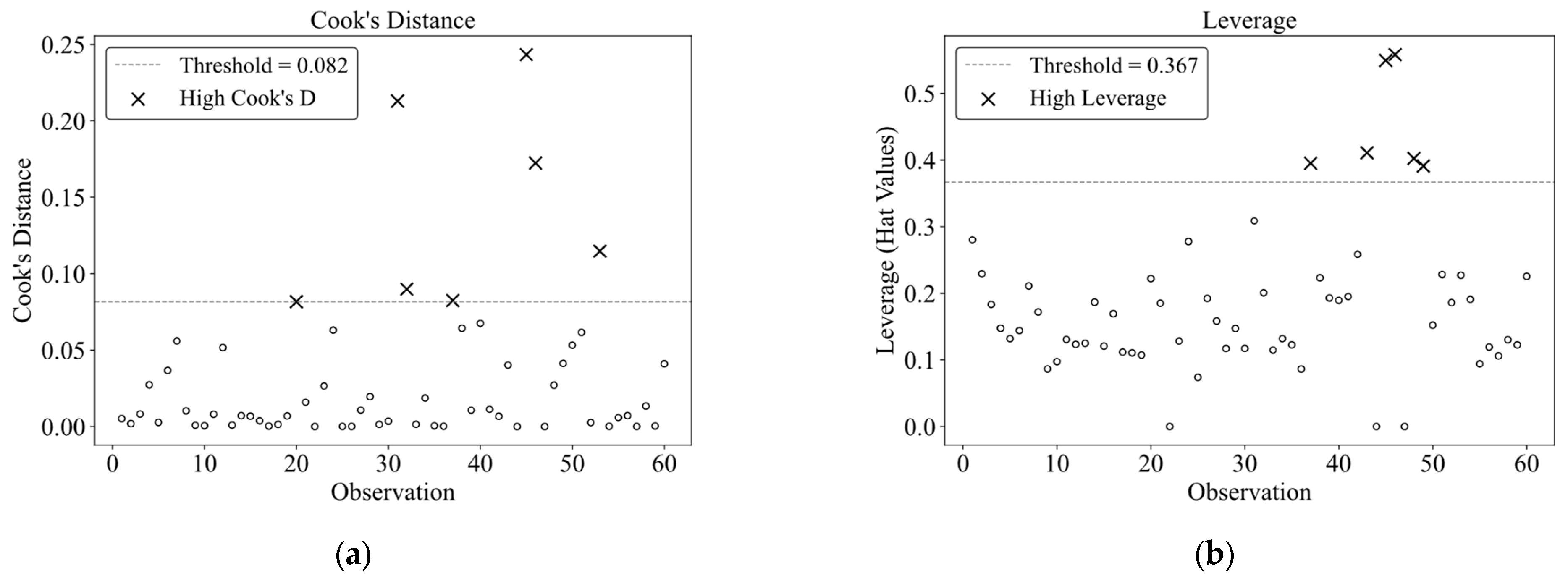
Figure A2.
(a) Sensitivity to the duration of a 10% MTL level increase (1–4 quarters); (b) sensitivity to lag structure under a temporary 1-quarter shock. Baseline: NARDL(3; 1, 1, 1, 1); second-best BIC: NARDL(3; 1, 1, 3, 1); lower-order AR: NARDL(2; 1, 1, 1, 1).
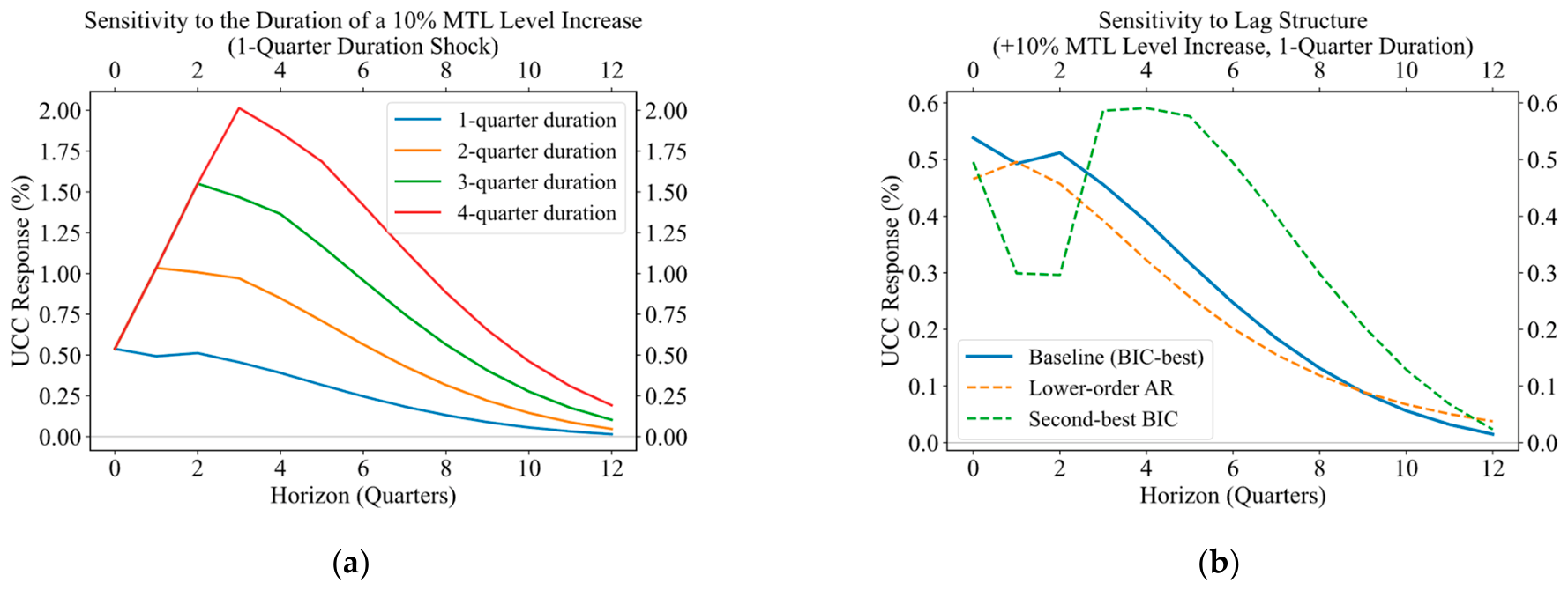
References
- Musarat, M.A.; Alaloul, W.S.; Liew, M. Impact of inflation rate on construction projects budget: A review. Ain Shams Eng. J. 2021, 12, 407–414. [Google Scholar] [CrossRef] [Scilit]
- Ali Musarat, M.; Salah Alaloul, W.; Liew, M.; Maqsoom, A.; Hannan Qureshi, A. Investigating the impact of inflation on building materials prices in construction industry. J. Build. Eng. 2020, 32, 101485. [Google Scholar] [CrossRef] [Scilit]
- Flyvbjerg, B.; Holm, M.S.; Buhl, S. Underestimating costs in public works projects: Error or lie? J. Am. Plan. Assoc. 2002, 68, 279–295. [Google Scholar] [CrossRef] [Scilit]
- Hamilton, J.D. Oil and the macroeconomy since World War II. J. Political Econ. 1983, 91, 228–248. [Google Scholar] [CrossRef] [Scilit]
- Kilian, L. Not all oil price shocks are alike: Disentangling demand and supply shocks in the crude oil market. Am. Econ. Rev. 2009, 99, 1053–1069. [Google Scholar] [CrossRef] [Scilit]
- Ashuri, B.; Lu, J. Time series analysis of ENR construction cost index. J. Constr. Eng. Manag. 2010, 136, 1227–1237. [Google Scholar] [CrossRef] [Scilit]
- Peltzman, S. Prices rise faster than they fall. J. Political Econ. 2000, 108, 466–502. [Google Scholar] [CrossRef] [Scilit]
- Shin, Y.; Yu, B.; Greenwood-Nimmo, M. Modelling asymmetric cointegration and dynamic multipliers in a nonlinear ARDL framework. In Festschrift in Honor of Peter Schmidt: Econometric Methods and Applications; Sickles, R.C., Horrace, W.C., Eds.; Springer: New York, NY, USA, 2014; pp. 281–314. [Google Scholar]
- Tang, K.; Xiong, W. Index investment and the financialization of commodities. Financ. Anal. J. 2012, 68, 54–74. [Google Scholar] [CrossRef] [Scilit]
- Cheng, I.-H.; Xiong, W. Financialization of commodity markets. Annu. Rev. Financ. Econ. 2014, 6, 419–441. [Google Scholar] [CrossRef] [Scilit]
- Baffes, J.; Kose, M.A.; Ohnsorge, F.; Stocker, M. The Great Plunge in Oil Prices: Causes, Consequences, and Policy Responses; (World Bank Policy Research Note No. PRN/15/01); World Bank: Washington, DC, USA, 2015. [Google Scholar]
- Akintoye, A.; Bowen, P.; Hardcastle, C. Macro-economic leading indicators of construction contract prices. Constr. Manag. Econ. 1998, 16, 159–175. [Google Scholar] [CrossRef] [Scilit]
- Ashuri, B.; Shahandashti, S.M.; Lu, J. Empirical tests for identifying leading indicators of ENR construction cost index. Constr. Manag. Econ. 2012, 30, 917–927. [Google Scholar] [CrossRef] [Scilit]
- Shahandashti, S.M.; Ashuri, B. Forecasting Engineering News-Record construction cost index using multivariate time series models. J. Constr. Eng. Manag. 2013, 139, 1237–1243. [Google Scholar] [CrossRef] [Scilit]
- Hwang, S. Time series models for forecasting construction costs using time series indexes. J. Constr. Eng. Manag. 2011, 137, 656–662. [Google Scholar] [CrossRef] [Scilit]
- Shahandashti, S.M.; Ashuri, B. Highway construction cost forecasting using vector error correction models. J. Manag. Eng. 2016, 32, 04015040. [Google Scholar] [CrossRef] [Scilit]
- Faghih, S.A.M.; Kashani, H. Forecasting construction material prices using vector error correction model. J. Constr. Eng. Manag. 2018, 144, 04018075. [Google Scholar] [CrossRef] [Scilit]
- Joukar, A.; Nahmens, I. Volatility forecast of construction cost index using general autoregressive conditional heteroskedastic method. J. Constr. Eng. Manag. 2016, 142, 04015051. [Google Scholar] [CrossRef] [Scilit]
- Shiha, A.; El-Adaway, I.H. Forecasting construction material prices using macroeconomic indicators of trading partners. J. Manag. Eng. 2024, 40, 04024036. [Google Scholar] [CrossRef] [Scilit]
- Liu, Q.; He, P.; Peng, S.; Wang, T.; Ma, J. A survey of data-driven construction materials price forecasting. Buildings 2024, 14, 3156. [Google Scholar] [CrossRef] [Scilit]
- Wang, J.; Qu, Z.; Lee, C.-Y.; Skitmore, M. Highway construction cost index forecasting: A hybrid VMD–LSTM–GRU method. Constr. Manag. Econ. 2025, 43, 849–863. [Google Scholar] [CrossRef] [Scilit]
- Wang, J.; Qu, Z.; Skitmore, M. Predicting construction cost index using a VMD-GRU framework with the MHSA mechanism. J. Constr. Eng. Manag. 2026, 152, 04025236. [Google Scholar] [CrossRef] [Scilit]
- Ma, M.; Tam, V.W.Y.; Le, K.N.; Osei-Kyei, R. A systematic literature review on price forecasting models in construction industry. Int. J. Constr. Manag. 2024, 24, 1191–1200. [Google Scholar] [CrossRef] [Scilit]
- Zheng, S.; Tan, Z.; Xing, W.; Zhou, X.; Zhao, P.; Yin, X.; Hu, H. A comparative exploration of the chaotic characteristics of Chinese and international copper futures prices. Resour. Policy 2022, 78, 102790. [Google Scholar] [CrossRef] [Scilit]
- Bacon, R.W. Rockets and feathers: The asymmetric speed of adjustment of UK retail gasoline prices to cost changes. Energy Econ. 1991, 13, 211–218. [Google Scholar] [CrossRef] [Scilit]
- Borenstein, S.; Cameron, A.C.; Gilbert, R. Do gasoline prices respond asymmetrically to crude oil price changes? Q. J. Econ. 1997, 112, 305–339. [Google Scholar] [CrossRef] [Scilit]
- Meyer, J.; von Cramon-Taubadel, S. Asymmetric price transmission: A survey. J. Agric. Econ. 2004, 55, 581–611. [Google Scholar] [CrossRef] [Scilit]
- Kilian, L.; Vigfusson, R.J. Are the responses of the U.S. economy asymmetric in energy price increases and decreases? Quant. Econ. 2011, 2, 419–453. [Google Scholar] [CrossRef] [Scilit]
- Flaaen, A.; Pierce, J. Disentangling the Effects of the 2018–2019 Tariffs on a Globally Connected U.S. Manufacturing Sector; Finance and Economics Discussion Series 2019-086; Board of Governors of the Federal Reserve System: Washington, DC, USA, 2019. [Google Scholar] [CrossRef] [Scilit]
- Carlton, D.W. The rigidity of prices. Am. Econ. Rev. 1986, 76, 637–658. [Google Scholar]
- Working, H. Note on the correlation of first differences of averages in a random chain. Econometrica 1960, 28, 916. [Google Scholar] [CrossRef] [Scilit]
- Wilson, J.D. Chinese resource security policies and the restructuring of the Asia-Pacific iron ore market. Resour. Policy 2012, 37, 331–339. [Google Scholar] [CrossRef] [Scilit]
- Wårell, L. The effect of a change in pricing regime on iron ore prices. Resour. Policy 2014, 41, 16–22. [Google Scholar] [CrossRef] [Scilit]
- Tong, H. Non-Linear Time Series: A Dynamical System Approach; Oxford University Press: Oxford, UK, 1990. [Google Scholar] [CrossRef] [Scilit]
- Teräsvirta, T. Specification, estimation, and evaluation of smooth transition autoregressive models. J. Am. Stat. Assoc. 1994, 89, 208–218. [Google Scholar] [CrossRef] [Scilit]
- van Dijk, D.; Teräsvirta, T.; Franses, P.H. Smooth transition autoregressive models—A survey of recent developments. Econom. Rev. 2002, 21, 1–47. [Google Scholar] [CrossRef] [Scilit]
- Pesaran, M.H.; Shin, Y.; Smith, R.J. Bounds testing approaches to the analysis of level relationships. J. Appl. Econom. 2001, 16, 289–326. [Google Scholar] [CrossRef] [Scilit]
- Narayan, P.K. The saving and investment nexus for China: Evidence from cointegration tests. Appl. Econ. 2005, 37, 1979–1990. [Google Scholar] [CrossRef] [Scilit]
- Lütkepohl, H. New Introduction to Multiple Time Series Analysis; Springer: Berlin/Heidelberg, Germany, 2005. [Google Scholar]
- Galeotti, M.; Lanza, A.; Manera, M. Rockets and feathers revisited: An international comparison on European gasoline markets. Energy Econ. 2003, 25, 175–190. [Google Scholar] [CrossRef] [Scilit]
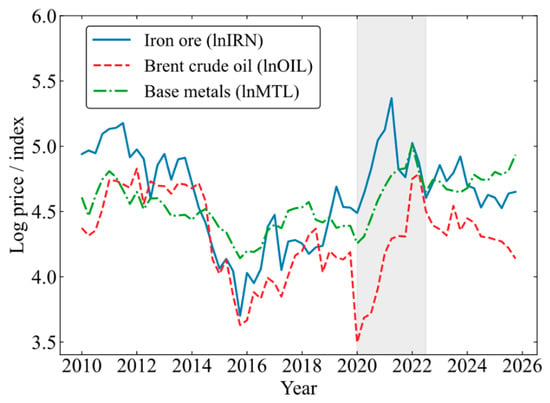
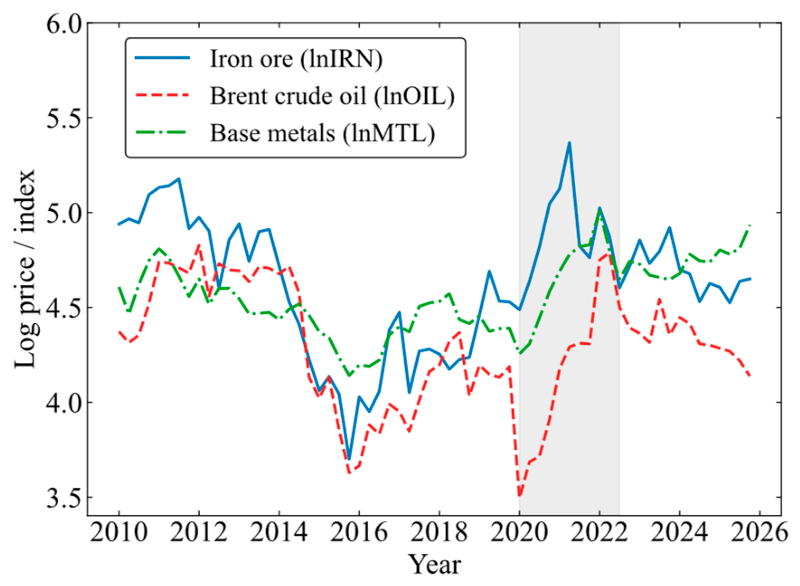
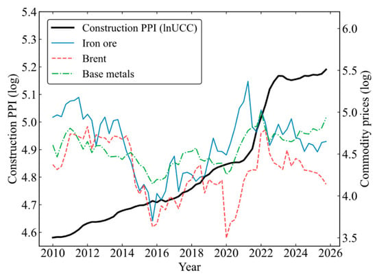
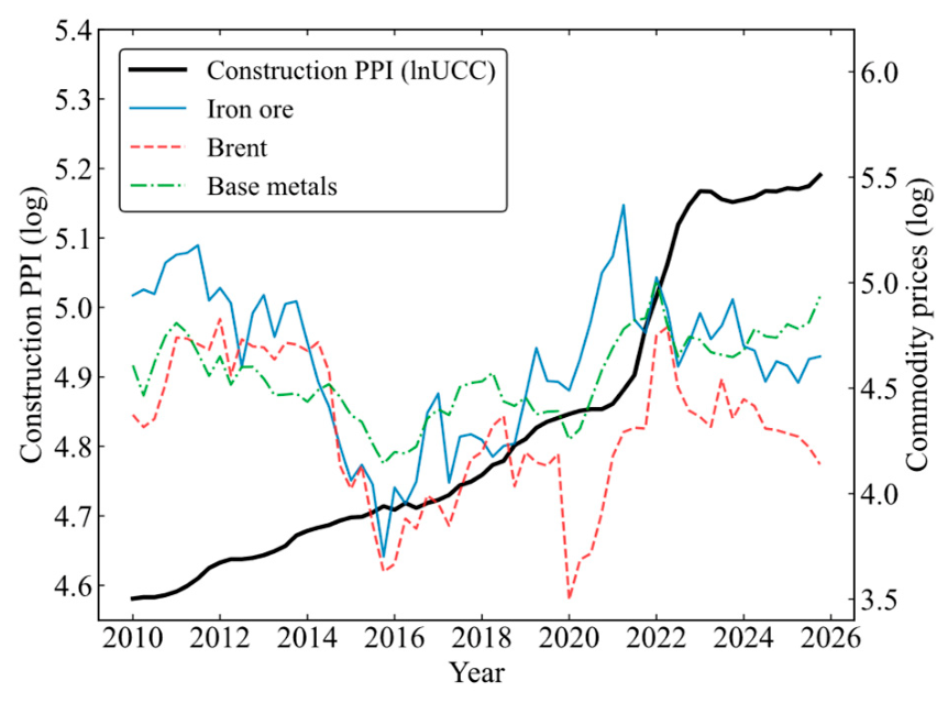
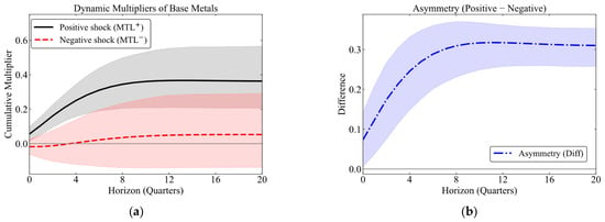
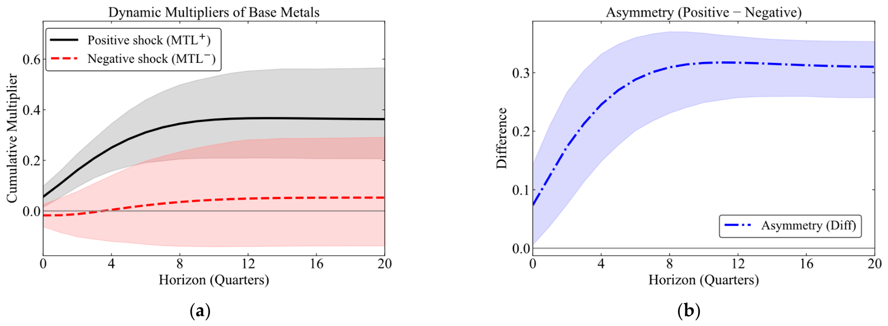
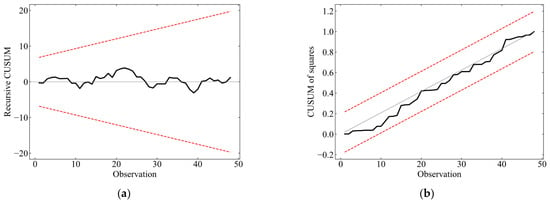
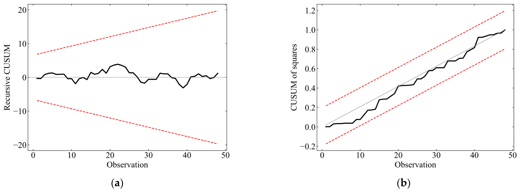
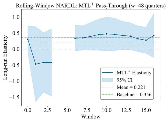
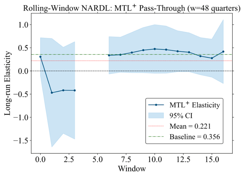
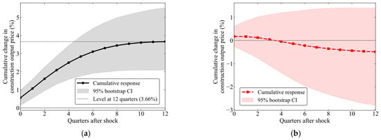
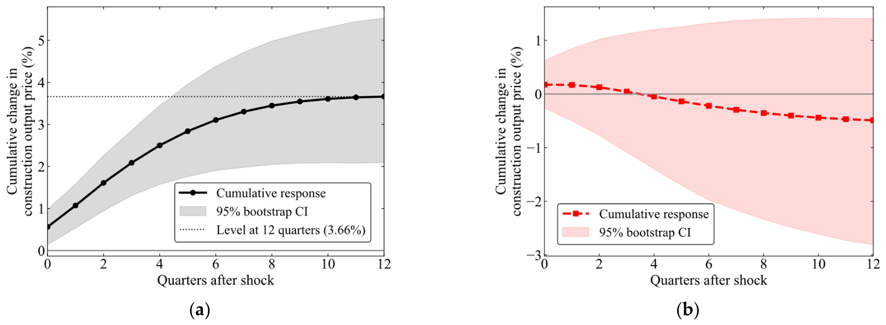

Disclaimer/Publisher’s Note: The statements, opinions and data contained in all publications are solely those of the individual author(s) and contributor(s) and not of MDPI and/or the editor(s). MDPI and/or the editor(s) disclaim responsibility for any injury to people or property resulting from any ideas, methods, instructions or products referred to in the content. |
© 2026 by the authors. Licensee MDPI, Basel, Switzerland. This article is an open access article distributed under the terms and conditions of the Creative Commons Attribution (CC BY) license.