


Abstract
Ward cooling is controlled by a single thermostat, yet whether it represents the mean room temperature is rarely evaluated. Existing virtual sensing reconstructs values at predetermined locations rather than identifying which location should be the reference. This study locates that reference point, tests its stability as the thermostat and occupant move, and estimates it from existing control signals. Air temperature and humidity were measured at 5-min intervals at 21 plan locations and three heights in a 16.03 m2 ward-type test room without mechanical ventilation, a 70 W heated cylinder as occupant, in six configurations. The instantaneous spatial deviation reached 4.5 °C. Against the room mean, the thermostat gave a slope of only 0.52 and read high by up to 0.86 °C, whereas one point gave 0.98 and was selected in five of six cases; training-window-only selection returned the same point. Estimating it from four control signals cut the thermostat’s tracking error by 41%, from 0.291 to 0.172 °C, and reproduced the point to within 0.222 °C when trained on five cases and tested on the sixth. Representativeness tracks the deviation field, which was invariant across configurations, so the point needs to be identified once per room. Comfort and energy were not measured.
1. Introduction
As greenhouse gas reduction has emerged as an international agenda in response to climate change, energy savings in the building sector have received increasing attention. The building and construction sector accounts for approximately 32% of global energy consumption [1]. Among building types, hospitals require year-round operation of air-conditioning systems to maintain a healing environment for patients and are subject to stringent indoor environmental requirements, making them more energy-intensive than other building types [2,3]. Within hospitals, inpatient wards account for a large share of heating and cooling energy owing to their long occupancy hours; improving the air-conditioning operation of ward spaces can therefore contribute directly to the overall energy savings of hospital buildings [4].
Research on energy savings in hospital buildings has proceeded along two broad directions. The first is a hardware-oriented approach, including improvements in envelope performance, the introduction of heat recovery systems, and the replacement of equipment with high-efficiency alternatives [2,3,4]. The second concerns operation and control, including sensor-network-based monitoring, IoT-based indoor environmental management, and artificial intelligence-based energy prediction and optimal control [5,6,7]. The latter approach commonly presupposes data collected from sensors installed in the building, and thus requires a stable and reliable sensing environment [8].
In practice, however, sensors are often not installed in sufficient numbers because of cost constraints, or are not replaced promptly after failure [9,10]. Virtual sensing has been proposed as a means of compensating for such limited sensing environments. Virtual sensing estimates a specific quantity without a physical sensor by exploiting the mathematical relationships among variables within a system [11], and in the building field it has been applied to the estimation of district heating energy consumption [12], occupancy information [13], flow rates in air-conditioning systems [14,15], and thermal comfort indices [16]. Its scope has recently expanded to sensor selection for indoor temperature monitoring [17], artificial intelligence-based virtual sensors in IoT environments [18], and deep learning-based virtual sensor modeling [19].
Existing studies on virtual sensing have focused on how to reconstruct a value whose location and physical meaning are already determined. Representative applications include the substitution of system variables [12,14,15,20], the observation of unmeasured information [13], and backup for fault diagnosis [21]; an approach that inversely computes local temperature using a physical model has also been proposed [22]. More recently, Kowli et al. [23] used the correlations among temperature and humidity measurements collected in a laboratory, a conference hall, and an office to determine where physical sensors should be deployed, and designed virtual sensors that estimate temperature and humidity at unsensed locations. That study demonstrated that the thermal distribution of an indoor space can be observed with a reduced number of sensors and shares a methodological basis with the present work. However, it evaluated only the fidelity of the reconstruction, leaving open which of the reconstructed locations is appropriate as a control reference and whether that appropriateness persists when indoor conditions change. In other words, although the existing studies are methodologically diverse, they share the premise that the location to be estimated is given in advance, and studies that treat the control reference point itself as an object of selection are difficult to find.
The influence of the selection of the temperature measurement location on control performance has been examined at the zone level. Li et al. [24] simulated a situation in which a single thermostat controls multiple zones in a multi-zone commercial building, and reported that cooling energy could increase by up to 17% or decrease by up to 12% relative to the baseline, heating energy could increase by up to 51% or decrease by up to 52%, and unmet hours for cooling could differ by as much as 1200 h depending on the sensor placement. Kontes et al. [25] further noted that the dry-bulb temperature measured at the thermostat location is not always an adequate proxy for thermal comfort, and that simple temperature limits alone are insufficient to guarantee comfort.
At the room scale, the problem has been approached both numerically and experimentally. Du et al. [26] coupled building energy simulation with computational fluid dynamics to optimize the position of a VAV temperature sensor and found that the conventional return-air position is not always the best choice. Chen and Gorlé [27] located temperature sensors under buoyancy-driven natural ventilation using computational fluid dynamics with uncertainty quantification, and Tian et al. [28] coupled airflow and system simulation to optimize thermostat placement at the design stage. These, like the physical-model approach of [22], obtain the reference from a computed field, which requires the boundary conditions of the space to be specified in advance. Measurement-based work has instead addressed the reading itself. Shinoda et al. [29] compared eleven commercial room temperature sensors in a climate chamber and found differences of up to 1.8 K between sensors at the same position, and of 1.5 to 2.5 K for the same sensor moved between positions under high load. Liu et al. [30] noted that determining a sensor position requires the space dimensions, the sensor specification, the type and location of the HVAC components, the envelope construction and the function of the space—information that is rarely assembled in practice. Suryanarayana et al. [31] derived sensor locations for multi-zone buildings from measured data rather than from a model.
However, Li et al. [24] addressed problems arising from load differences between zones with different orientations, window areas, and occupancy conditions, and did not consider the deviations that arise within a single zone from airflow and heat source placement.
In actual buildings, heating and cooling systems are typically controlled based on the reading of a single thermostat per space, with the implicit assumption that the value at that point represents the entire space. Thermostat locations, however, are often determined by the convenience of wiring and installation, and it has been pointed out that the relevant standards do not provide practical recommendations on placement [24]. Field studies on vertical thermal stratification have been conducted mainly in large spaces such as gymnasiums and atria [32], and whether deviations large enough to affect the selection of a control reference point occur in single rooms has received limited attention. Ward spaces are particularly relevant in this respect, because occupants remain in a supine posture on a bed for extended periods and cannot readily change their position, so that the thermal environment at a specific location is directly attributable to the occupant. Surveys of patients with restricted mobility support this premise. Zhen et al. [33] found bed-lying patients to prefer markedly warmer conditions than their accompanying family members, and Sun et al. [34] found orthopedic patients to be more sensitive to changes in the thermal environment than healthy occupants, with neutral standard effective temperatures of 17.7 °C and 21.7 °C, respectively. Alotaibi et al. [35] measured 120 patients in air-conditioned wards and concluded that a single centrally set room condition is unlikely to suit a patient population, and Lomas and Giridharan [36] recorded ward temperatures across successive summers and assessed them against comfort standards. These studies characterize the environment at the room scale, but which point within a room the control system should read has not been examined in this setting.
One reason such examination has been limited is the practical constraint that simultaneous measurement at numerous locations is required to assess spatial representativeness.
In this study, sensors were installed at 21 plan locations and three heights in a laboratory space configured to emulate a hospital ward, and temperature and relative humidity were measured at high spatial density. At 16 of these locations, thermocouples were arranged in a 4 × 4 grid to measure temperature at 48 points, while thermo-hygrometers were installed at the remaining five locations to measure temperature and relative humidity at 15 points, of which 13 remained valid for the humidity analysis (Section 2.2). The surface temperatures of the walls, ceiling, and floor, as well as the FCU inlet and outlet and outdoor conditions, were acquired concurrently.
Four aspects were addressed for six cases differing in the positions of the thermostat and the heat source. First, the structure of the indoor temperature and humidity deviations was characterized by decomposing them by height. Second, the arithmetic mean of the 48 points was defined as the spatial mean; the point closest to it was selected as the representative point, and its representativeness was compared with that of the existing thermostat through regression analysis. Third, whether the location and representativeness of the representative point are maintained under varying thermostat and occupant positions was examined, and the results were interpreted in relation to the indoor airflow structure. Fourth, a virtual sensor that estimates the temperature and humidity at the representative point using only the minimum set of input variables already available on site was constructed, and its performance was verified.
The contributions of this study are as follows.
- Field measurement data on the temperature and humidity distribution in a ward-type space were obtained at high spatial density for six cases. Temperature was acquired at 48 points and relative humidity at 15 points, of which 13 remained valid, at 5-min intervals, together with indoor surface temperatures and system-side boundary conditions.
- Under ward conditions, temperature deviation arose mainly from horizontal non-uniformity at bed level, reaching 4.5 °C, whereas relative humidity remained considerably more uniform. The representativeness problem is therefore concentrated in the variable on which the system is actually controlled.
- The spatial representativeness of the thermostat varied with its installation location and with the occupant position, whereas the point representing the room remained stable regardless of these changes. The deviation field itself proved invariant across configurations, indicating that the representative point is determined by room characteristics rather than by the placement of the thermostat or the occupant.
- Taking the representative point as a virtual thermostat, it was estimated from four variables already available from the existing control system, and a linear model alone provided sufficient accuracy.
2. Materials and Methods
2.1. Test Space and Experimental Conditions
The measurements were conducted in a single-story experimental building located in Gwangju, Republic of Korea. The building is an educational and research facility with a floor area of 196 m2, partitioned internally into a meeting room, five testbeds, and a mechanical room, each accessed from a corridor on the north side (Figure 1a). Testbed 1 (16.03 m2, 2.85 m × 5.625 m, ceiling height 2.7 m) was selected as the target space. An overview of the building is given in Table 1.
Figure 1.
Test building: (a) floor plan; (b) interior view of Testbed 1.
Table 1.
Overview of the test building.
Testbed 1 has an entrance door on the north side leading to the corridor and a window with a blind on the south side. Cooling is provided by supplying chilled water generated by an air-to-water heat pump (AWHP) to a ceiling-type fan coil unit (FCU), which is installed on the northeast ceiling and discharges toward the interior of the room. During the measurement period of this study, no dedicated mechanical ventilation system was installed, so the indoor airflow was formed solely by the circulation induced by the FCU.
The target space was configured to emulate the operating conditions of a single-occupancy ward in a general inpatient unit. Reflecting the air-conditioning operation pattern of ward spaces, the FCU was operated continuously for 24 h, and the cooling setpoint was maintained at 24 °C with reference to ANSI/ASHRAE/ASHE Standard 170-2017 [37]. Control is of the on–off type with a deadband of ±0.5 °C about the setpoint. A folding bed was placed inside the room (Figure 1b).
To examine whether the data-driven model generalizes across varying indoor conditions, six cases were established by changing the positions of the thermostat and the heat source. The thermostat was placed at one of the three locations indicated in Figure 2a: ① adjacent to the entrance door, ② at the center of the east wall, and ③ at the center of the west wall, all installed at 1.2 m above the floor. Location ① reflects the common practice in actual buildings of installing thermostats next to the door for wiring convenience.
Figure 2.
Sensor arrangement in Testbed 1: (a) plan view; (b) three-dimensional view.
Human heat gain was represented by a cylindrical element wound with a heating wire, with a heat output of 70 W corresponding to the sensible heat release of one occupant. It was placed on the bed surface at one of the same three locations, 0.3 m from the wall, laid horizontally along the long axis of the bed to approximate the posture of a supine occupant. In Cases 4 and 6, the thermostat and the heat source were placed at the same location to emulate the situation in which an occupant stays near the thermostat and operates it directly. The six cases therefore vary two factors separately: the position of the thermostat, which determines what the control sensor reads, and the proximity of the occupant to it, which determines how much local heat gain that reading carries.
The setpoint, operating schedule, and number of occupants were kept identical across all cases so that only the effect of positional changes was isolated. For each case, four days of data were used for analysis after a stabilization period following the reconfiguration. For some cases, an additional day was measured later under the same configuration to compensate for missing data, and this day was included to form the four-day dataset. The results were verified to be insensitive to the inclusion of these re-measured days: excluding the re-measured day from each of the four cases that contain one gives a mean thermostat slope of 0.522 and a mean representative-point slope of 0.972, against 0.523 and 0.976 for the full four-day dataset. The conditions and analysis periods for each case are given in Table 2.
Table 2.
Experimental conditions and analysis periods *.
2.2. Sensor Configuration and Measurement
The measurement system was installed and commissioned on 1 July 2024, and the six cases analyzed here were recorded between 30 July and 2 September 2024. The measured variables were dry-bulb temperature and relative humidity, recorded at 5-min intervals. For each case, the analysis used four days of data (5760 min, 1152 records) during which the configuration was maintained, and no data were missing.
Indoor temperature distribution was measured using K-type thermocouples, with readings acquired through a data logger (GL840-WV, Graphtec Corporation, Yokohama, Japan). Sensors were arranged at 16 locations in a 4 × 4 grid in plan, with three heights at each location, giving 48 measurement points in total. The grid columns were designated A–D from west to east, and the positions 1–4 from the north side, where the entrance door is located toward the window side; the third index denotes the height. For example, A-4-2 refers to the sensor installed at the mid-height of the window-side position in the westernmost column. The sensor spacing was 0.70 m in the east–west direction and 1.475 m in the north–south direction, with clearances of 0.37 m and 0.60 m from the walls, respectively.
The sensor heights were determined to reflect the occupancy characteristics of ward spaces. Because patients, the primary occupants of inpatient units, spend most of their time lying on a bed, 0.6 m—corresponding to the upper surface of the bed—was set as the primary evaluation height. To this were added 1.7 m, the head height of standing medical staff and visitors, and 2.1 m, which characterizes the air in the upper part of the occupied zone; the height indices 1, 2, and 3 correspond to these levels, respectively (Figure 2b). The uppermost sensor (2.1 m) is located 0.6 m below the ceiling (2.7 m) to avoid the direct influence of the discharge airflow from the ceiling-mounted FCU and of the ceiling boundary layer. The ankle height (0.1 m) used in ISO 7730:2005 [38] and ANSI/ASHRAE Standard 55-2023 [39] for evaluating vertical air temperature differences corresponds to the region beneath the bed, to which occupants are not actually exposed, and was therefore excluded from the measurement.
Because relative humidity cannot be measured with thermocouples, separate thermo-hygrometers (Testo Saveris 2-H2, Testo SE&Co. KGaA, Titisee-Neustadt, Germany) were used. They were placed between the north–south grid columns so as not to interfere with the thermocouple stands, in three rows: between positions 1 and 2 (row a), between positions 2 and 3 (row b), and between positions 3 and 4 (row c). Rows a and c each held one unit on the west (W) and one on the east (E) side, and row b held one unit at the center (M) of the room. At each location, sensors were installed at the same three heights as the thermocouples, giving 15 measurement points for temperature and relative humidity. The thermo-hygrometers follow the same index order as the thermocouples—east–west position, north–south row, and height—so that W-c-2, for example, denotes the sensor on the west side of row c at mid-height. The spatial measurement resolution for relative humidity is therefore lower than that for temperature, which was considered in the interpretation of the results.
Separately, thermo-hygrometers (TR-72wf-S, T&D Corporation, Matsumoto, Nagano, Japan) were used to measure the temperature and humidity of the outdoor air, the FCU inlet, the FCU outlet, and the adjacent corridor. The room temperature sensor of the thermostat is detachable from the unit and can be relocated; it was installed at the location specified for each case, and its reading was acquired directly. The measurement ranges and accuracies of the sensors are given in Table 3.
Table 3.
Specifications of the sensors used in the measurement.
The accuracies listed in Table 3 refer to the absolute accuracy of individual channels, whereas the analysis in this study rests on differences between points measured simultaneously. Systematic components, including the reference junction compensation error, act commonly on all channels connected to the same logger and therefore cancel in the inter-channel differences. Rather than calibrating each channel against a reference standard, the channel-specific component that remains was assessed from the measurements themselves. The time-averaged deviation of each channel from the spatial mean reproduces between the six cases with a standard deviation of 0.079 °C, and 0.033 °C at the representative point, an order of magnitude below the absolute accuracy listed in Table 3; it is this component, rather than the absolute accuracy, that propagates into a difference between channels. Drift was assessed in the same way: the agreement between the deviation fields of any two cases shows no relationship with the interval separating them, the correlation between the two being −0.11 over separations of 4 to 24 days, so no systematic drift is evident. This characterizes the reproducibility of each channel rather than its agreement with the others; a constant offset in a channel would not be detected in this way, but neither does it enter the comparisons between cases on which the analysis rests. The thermocouples were used with a full-scale range of 100 °C, for which the measurement resolution is 0.01 °C.
Two of the fifteen thermo-hygrometers, those at 1.7 m and 2.1 m at the central location, degraded over the measurement campaign and were excluded from the humidity analysis. Their readings drifted upward relative to the other four locations from early August onward and eventually saturated: the unit at 2.1 m reported exactly 100.0% RH for 3% of the day on 7 August, rising to 58% by 21 August, and the unit at 1.7 m began to clip from 23 August. The drift followed calendar time rather than the experimental configuration—a day re-measured on 1 September under the Case 1 configuration showed an excess of +11.3% RH over the other four locations at 2.1 m, against +6.4 to +7.9% RH on the original Case 1 days of 30 July to 1 August—so a genuine feature of the central location can be excluded. The humidity analysis therefore uses the remaining 13 points. The unit at 0.6 m at the same location showed no saturation and was retained. Temperature results are unaffected, as the spatial mean and the representative point are computed from the 48 thermocouples alone.
2.3. Representative Point and Evaluation Metrics
When indoor temperature and humidity are not spatially uniform, the reading at a single point cannot readily represent the entire space. It is therefore necessary to define a representative point that serves as the control reference and to evaluate its representativeness quantitatively.
Throughout this paper, the instantaneous spatial deviation denotes the difference between the maximum and the minimum reading among the measurement points at a given instant; its maximum and its mean over the analysis period are reported separately.
The spatial mean temperature was defined as the criterion representing the thermal environment of the room. It was calculated as the arithmetic mean of the readings from the 48 thermocouples, as given in Equation (1).
Only the 48 thermocouples arranged in a uniform grid were used to compute the spatial mean. The thermo-hygrometers are positioned between the thermocouple grid points and are therefore spatially non-uniform, and they belong to a different instrument family in which a systematic offset may exist; they were consequently excluded from the calculation of the spatial mean.
The representative point, i*, was selected as the location with the smallest mean absolute error relative to the spatial mean over the entire measurement period, as given in Equation (2).
where i denotes a candidate location, Ti(t) the temperature measured at location i at time t, and N the number of measurement instants. The candidate locations comprised the same 48 thermocouple positions used to compute the spatial mean. Candidates were additionally assessed by the standard deviation of their mean deviation across the six cases, so that a point which happens to lie near the spatial mean in one configuration but not in others is not selected. The representative point for relative humidity was selected in the same manner among the 13 valid thermo-hygrometer points (Section 2.2).
Considering that occupants of a ward remain in a supine posture on a bed, the mean at the occupied height may also be adopted as the criterion instead of the mean over the entire room. To examine the influence of this choice on the results, the case in which the mean of the 16 points on the 0.6 m plane was used as the criterion was also computed for comparison.
The extent to which the selected representative point and the existing thermostat track the spatial mean was evaluated using the linear regression model given in Equation (3).
where Tj(t) denotes the value at the evaluated location (j = representative point or thermostat), a and b are the regression slope and intercept, respectively, and ε is the residual. A slope closer to unity and an intercept closer to zero indicate that the location tracks the variation in the spatial mean more closely, and the explanatory power of this tracking was evaluated using the coefficient of determination R2. The absolute difference from the spatial mean was additionally quantified using the mean absolute error (MAE).
The thermostat is mounted on the wall at 1.2 m and therefore measures under conditions different from those of the grid representing the room, so the difference between the two values may include a constant offset. The slope and R2 are invariant to a constant offset and are thus unaffected, whereas the mean absolute error is not. A bias-corrected mean absolute error (MAE*) was therefore computed as in Equation (4) and used for comparison.
where and denote the period means of the evaluated series and of the spatial mean, respectively. This metric removes any constant offset between the two series and compares only their fluctuating components.
2.4. Virtual Sensing Models
Estimating the temperature and humidity at the representative point requires an appropriate selection of input variables. Including variables weakly related to the prediction target enlarges the model unnecessarily and hinders training; both correlation and on-site applicability were therefore considered.
Pearson correlation coefficients between the representative point and the candidate variables were first computed using the entire measurement dataset from the six cases (6912 records in total) (Table 4). For temperature, the FCU outlet (0.83), the thermostat (0.70), and the FCU inlet (0.69) correlated most strongly, whereas solar radiation (0.33), the outdoor air (0.31), and the adjacent corridor (0.11) correlated weakly. For relative humidity, nearly all variables correlated strongly because indoor and outdoor humidity vary together in summer, with the FCU outlet (0.99), the thermostat (0.99), and the FCU inlet (0.95) being the highest.
Table 4.
Pearson correlation coefficients between the representative point and the candidate input variables, computed over the pooled dataset of the six cases (6912 records).
Among the remaining variables, a minimum set was selected by giving priority to whether sensor installation is feasible at the location when applied to actual buildings. Four input variables were finally selected: time, the thermostat, the FCU inlet, and the FCU outlet. These four quantities are referred to hereafter as control-system variables, in the sense that they are already available from the existing control system or from the vicinity of the indoor unit and therefore require no additional sensor installation. The time variable correlates weakly with the representative point but was included to reflect the temporal variation characteristics of indoor temperature and humidity in the model. Separate models were built for temperature and relative humidity. Both draw on the same three locations—the thermostat, the FCU inlet, and the FCU outlet—but the temperature model takes the temperatures at those locations as inputs, while the humidity model takes the relative humidities at the same locations. Because the thermostat position differs across cases, the reading at the corresponding position was used for each case. All input variables were min–max normalized before training to equalize their scales. To examine the influence of the number of input variables on prediction performance, the combinations were expanded sequentially in order of on-site availability: the two-variable combination comprised time and the thermostat, the three-variable combination added the FCU inlet, and the four-variable combination added the FCU outlet.
Multiple linear regression (MLR) was adopted as the primary virtual sensing model. Linear regression is insensitive to noise, less prone to overfitting, and algorithmically simple, and is therefore often preferred over complex nonlinear models when applied to real systems. It estimates the relationship between multiple independent variables and a single dependent variable under the assumption of linearity, as expressed in Equation (5).
where ŷ denotes the estimated temperature or relative humidity at the representative point, xk the k-th input variable, ωk its weight, ω0 the bias, and K the number of input variables.
A linear model alone, however, may be limited in capturing complex patterns within the data. A multi-layer perceptron (MLP), which can reflect nonlinear relationships, was therefore implemented alongside the linear model to examine the adequacy of the latter. The selected input variables were assigned to the input layer and the temperature or relative humidity at the representative point to the output layer. Three hidden layers with 32 neurons each were used, with ReLU as the activation function in the hidden layers and a linear function in the output layer. Adam was used as the optimizer and the mean squared error as the loss function, and the output values were also normalized before training.
A gain-and-offset recalibration of the thermostat was included as a baseline. It is the special case of Equation (5) with K = 1, written out in Equation (6), and uses no signal beyond the one the controller already reads. It separates the part of the improvement that comes from correcting the thermostat reading from the part that comes from the additional inputs.
where is the thermostat reading, and a and b are the gain and offset fitted on the training records.
Two further model families were included. Support vector regression (SVR) was implemented with a radial basis function kernel, a penalty parameter C = 10, an insensitive band ε = 0.02, and the scale heuristic for the kernel width γ. A random forest was implemented with 300 regression trees grown on bootstrap resamples with no depth limit. Both use the same four input variables as the models above. SVR uses the same min–max normalization; a random forest does not require input scaling. SVR is included because it reaches its solution by convex optimization rather than by iterative gradient descent, and therefore does not share the sensitivity of a neural network to the size of the training set. Both families are common baselines for indoor temperature estimation: Xu et al. [40] compared support vector machines, decision trees and neural networks for short-term indoor temperature prediction and Alawadi et al. [41] ranked 36 regressors for indoor temperature forecasting and found tree ensembles to lead, with support vector regression among the ten best.
The analyses were carried out in MATLAB R2025b (The MathWorks, Inc., Natick, MA, USA) and in Python 3.11 (Python Software Foundation, Wilmington, DE, USA) with scikit-learn 1.8.0.
The training settings of all five models are summarized in Table 5. Because the thermostat location differs across cases, the models were trained and validated independently for each case, and the performance is reported as the mean over the six cases. Section 3.4 reports a second protocol, in which the model is fitted on five cases and evaluated on the sixth.
Table 5.
Training configuration of the prediction models.
Given the limited measurement period, the dataset of each case was split chronologically without shuffling: the first 806 records (70%) were used for training and the last 346 (30%) for testing (Figure 3a). Preserving the temporal order avoids the leakage that random splitting would introduce into a time series and keeps the evaluation period disjoint from the training period. The MLP and the random forest were trained from three random initializations and the reported values are the means over those runs.
Figure 3.
Data splitting protocols. (a) Chronological train–test split within each case, used in Section 3.3. (b) Leave-one-case-out protocol used in Section 3.4, each case serving in turn as the held-out case.
Model performance was evaluated using the mean absolute error (MAE) and the root mean square error (RMSE), given in Equations (7) and (8).
where is the measured value at the representative point and the model estimate. In addition, the regression model in Equation (3) was applied to the virtual sensor estimates so that their tracking of the spatial mean could be compared with that of the thermostat and of the measured representative point.
3. Results
3.1. Spatial Distribution of Temperature and Humidity
Across all six cases, the instantaneous spatial deviation of indoor air temperature reached 4.5 °C with a mean of 2.1 °C. Even though the cooling setpoint was maintained at 24 °C and the occupancy conditions were held identical, temperature differences among indoor locations persisted at any given instant.
To identify where this deviation originates, it was decomposed by height (Table 6). The deviation on the 0.6 m plane, corresponding to bed level, reached 4.5 °C with a mean of 1.97 °C, almost the same as the overall deviation, whereas the 1.7 m and 2.1 m planes averaged only 1.22 °C and 1.46 °C, respectively. Most of the observed spatial deviation therefore originated not from vertical stratification but from horizontal non-uniformity at bed level.
Table 6.
Instantaneous spatial deviation of indoor air temperature and relative humidity by measurement height, averaged over the six cases *.
Relative humidity was considerably more uniform. The mean deviation over all heights was 8.7% RH, and the plane-averaged values differed by only 3.0% RH across the three heights (Table 6). A mild increase toward the ceiling is present, consistent with the absence of mechanical ventilation limiting air circulation in the upper part of the room where the influence of the FCU discharge airflow is weak, but it is small relative to the temperature deviation. The spatial representativeness problem addressed in this study is specific to temperature, the variable on which the system is controlled.
Examining the spatial distribution of indoor temperature by location (Figure 4), points B-1 and C-1 at bed level, in the northern part of the two central columns beneath the FCU discharge, were the lowest relative to the spatial mean, at −0.96 and −0.89 °C. At the 1.7 m height, the low-temperature region extended to B-2, B-3, C-2 and C-3, with deviations of −0.38 to −0.50 °C. Columns A and D adjacent to the side walls were warmer than the spatial mean, and the deviation was lowest on the north side and highest toward the south window. This reflects a structure in which the FCU discharge airflow enters and spreads along the central part of the room.
Figure 4.
Spatial deviation of indoor air temperature from the spatial mean at three measurement heights, averaged over the six cases: (a) 0.6 m (bed level); (b) 1.7 m; (c) 2.1 m. Columns A–D denote the west-to-east grid lines and rows 1–4 the north-to-south positions; the panels are drawn to the actual room proportions (2.85 m × 5.625 m). The boxed cell in (b) indicates the representative point identified in Section 3.2.
Relative to the spatial mean, the north wall deviated most (+4.30 °C) and the ceiling next (+2.83 °C); the remaining surfaces lay between +0.99 and +1.44 °C. Although all surfaces remained warmer than the indoor air, the air temperature directly beneath the FCU outlet was the lowest, indicating that the cooling effect of the discharge airflow outweighs the influence of the surrounding surfaces.
3.2. Spatial Representativeness of the Thermostat and the Representative Point
Before evaluating how individual points represent the room, the structure of the deviation field itself was examined. The 48-point deviation field was compared between every pair of the six cases, giving a mean correlation of 0.911 (0.800 to 0.995), so the pattern of which locations run warm and which run cool is essentially a property of the room rather than of the thermostat or heat-source arrangement (Figure 5). The cold region beneath the FCU discharge at B-1 and C-1 and the warm region along the window-side row appear in every case with comparable magnitude, even though the thermostat and the heat source were relocated between the entrance door, the east wall and the west wall. Ordering the 48 points by their mean deviation shows the same result pointwise: the spread across cases at each point is narrow, and it is narrowest where the field vanishes (Figure 6). Because the field itself is invariant, the point at which it vanishes is invariant as well, and a location that represents the room in one configuration will continue to do so in another. The following analysis identifies that point and compares it with the existing thermostat.
Figure 5.
Invariance of the temperature deviation field across the six configurations. Time-averaged deviation from the 48-point spatial mean at each plan position, for the three measurement heights (rows) and the six cases (columns). Panels are drawn to the actual room proportions (2.85 m × 5.625 m), with north (entrance door) at the top and south (window) at the bottom; the boxed cell marks the column containing the representative point A-4. Black squares denote the thermostat and red circles the heat source, placed at ① the entrance door, ② the center of the east wall, or ③ the center of the west wall as listed in Table 2. Although these positions differ between cases, the pattern of warm and cool locations is essentially unchanged.
Figure 6.
The 48 measurement points ordered by their mean deviation from the spatial mean, with the value of each case overlaid. The narrow vertical spread at each point reflects the invariance of the deviation field, for which the mean pairwise correlation between cases was 0.911. Vertical bars show ±1 SD across the six cases for the selected representative point A-4-2 (red) and the two nearest competing candidates, which have a mean deviation closer to zero but a wider spread across cases.
To examine how well the existing thermostat represents the room under spatially non-uniform conditions, a regression analysis against the spatial mean was performed (Figure 7, Table 7).
Figure 7.
Regression of the thermostat reading and the representative point against the spatial mean temperature for each case. The representative point is A-4-2 in all six cases. The dotted diagonal denotes the 1:1 line.
Table 7.
Regression of the thermostat reading and the representative point against the spatial mean temperature †.
The slope of the thermostat ranged from 0.370 to 0.683 across the six cases, with a mean of 0.523. This indicates that when the spatial mean varies by 1 °C, the thermostat reading changes by only 0.52 °C, detecting approximately half of the temperature variation in the room. The R2 was likewise low, averaging 0.534.
The thermostat readings exceeded the spatial mean in all cases, with a mean difference of +0.62 °C. The difference was largest in Cases 4 and 6, at +0.84 °C and +0.86 °C, respectively; in these two cases, the heat source was placed at the same location as the thermostat. When an occupant stays near the thermostat, the local heat gain inflates the sensed temperature, and the loop continues to call for cooling after the room average has already fallen below the setpoint. The offset common to all cases includes a component attributable to the mounting height of the thermostat, whereas the differences between cases were obtained with the same sensor at the same height and only the heat source was relocated; therefore, they are attributed to the proximity of the occupant.
The offset does not stem from insufficient capacity or control failure. The thermostat cycled down to 23.7–23.9 °C at the bottom of each cycle in every case, and the spatial mean ranged from 23.36 to 23.89 °C, below the setpoint throughout; had the capacity been inadequate, the room would have remained above it.
The condition in which the thermostat read at or above the setpoint while the spatial mean stayed below it accounted for 47.3–65.1% of the measurement period and was most frequent in Cases 4 and 6 at 63.0% and 65.1%, where the heat source shared the location of the thermostat. The offset is therefore attributable to the difference between the temperature sensed at the thermostat location and the room average.
The representativeness of the thermostat also varied with its position relative to the FCU outlet. Case 6, with the lowest slope (0.370), placed the thermostat on the west wall, farthest from the northeast side where the FCU is installed. As shown in Figure 4, the west column remains warmer than the spatial mean at all heights, a pattern consistent with a stagnant region in which the influence of the discharge airflow is weak. Air velocity was not measured, so this characterization of the flow field is inferred from the temperature distribution. At such a location, the temperature variation in the room is not sufficiently transmitted to the thermostat, and the additional influence of the adjacent heat source resulted in the lowest slope and R2 among all cases.
In contrast, when the point closest to the spatial mean was selected as the representative point, the same location, A-4-2, was identified in five of the six cases. In the remaining case, a nearby point in the same column gave a marginally smaller error, but applying A-4-2 to all cases increased the error by only 0.034 °C, and Table 7 and Figure 7 therefore report A-4-2 throughout. Its slope against the spatial mean ranged from 0.900 to 1.060 with a mean of 0.976, and its mean difference from the spatial mean was +0.03 °C, so that it tracked the variation in the spatial mean almost exactly; whereas the slope of the thermostat varied from 0.370 to 0.683 with the installation and occupant positions, that of the representative point stayed close to unity in all six. Among the 48 candidates, A-4-2 combined the smallest mean deviation with by far the smallest variation across cases; the next-ranked points matched it on one criterion but not on the other. The differences between the leading candidates are comparable to the reproducibility of an individual channel, so the selection identifies a region of the room rather than a uniquely optimal point. Selection of a representative point should therefore consider stability across conditions in addition to proximity to the spatial mean.
The point was selected using the whole record, so the statistics above include the data on which the selection was made. Repeating the selection on the training window of each case, the first 806 records, returns the same location. Evaluated on the held-out records, its RMSE against the spatial mean is 0.185 °C, second among the 48 candidates and 0.005 °C above the point that would have been selected with hindsight, so the selection contributes little to the reported performance.
The representative point A-4-2 corresponds to the mid-height (1.7 m) of the window-side position adjacent to the west wall, diagonally opposite the northeast corner where the FCU is installed and thus the farthest point in the room from it. As seen in Figure 4, this point lies in the part of the room least affected by the discharge airflow, at a height unaffected by the floor and ceiling boundary layers. The deviations from the spatial mean at the three heights were +0.14, +0.03, and +0.13 °C, the smallest at mid-height, which likewise reflects this structure.
The influence of the criterion used for selecting the representative point was also examined by adopting the mean of the 16 points on the 0.6 m plane, corresponding to the occupied height. The selected point shifted to D-4-2 in five of the six cases, still the mid-height (1.7 m) of window-side position 4, the row farthest from the FCU outlet, on the opposite side across the width of the room. Moreover, the difference between the whole-room mean and the occupied-height mean was 0.06 to 0.10 °C, negligible compared with the spatial deviation (mean 2.1 °C). The specific point therefore depends on the definition of the mean, whereas the region in which the representative point lies does not. Section 3.5 extends this comparison to a reference defined over the space occupied by the patient.
The same procedure applied to relative humidity identified E-c-1 in all six cases, with a regression slope against the humidity spatial mean ranging from 1.006 to 1.125 and an R2 of 0.987 to 0.997. Unlike temperature, where one case selected a different point, the humidity representative point was invariant across all six configurations, which is consistent with the small spatial deviation reported in Section 3.1.
3.3. Virtual Sensing of the Representative Point
The quantity a control system is required to hold at the setpoint is referred to here as the control reference, and the representative point of Section 3.2 is a location at which that reference can be read. Neither can carry a permanent sensor in an occupied ward: the representative point lies in open air rather than on a wall, where a thermostat would normally be mounted, and a reference defined over the occupied zone would require a sensor beside the occupant. A virtual sensor was therefore constructed to estimate the temperature and humidity at the representative point from the four control-system variables alone. Because the estimate is formed from signals rather than from an instrument at a fixed location, the same construction applies to the reference itself, as Section 3.5 shows. The prediction performance as a function of the number of input variables is shown in Figure 8. For both temperature and relative humidity, the error decreased on average as the number of input variables increased, although the improvement was not monotonic in every individual case. With four variables, the MAE of the MLR model was 0.247 °C for temperature and 0.570% RH for relative humidity, corresponding to improvements of approximately 19.5% and 33.1%, respectively, relative to the two-variable case.
Figure 8.
Prediction performance of the virtual sensor as a function of the number of input variables: (a) temperature (target A-4-2); (b) relative humidity (target E-c-1). Variables were added in the order of on-site availability: time and thermostat (2 inputs), plus FCU inlet (3 inputs), plus FCU outlet (4 inputs). Solid lines denote RMSE and dashed lines denote MAE. MLP values are means over three random seeds.
The variables that contributed most differed between temperature and relative humidity (Figure 8). For temperature, adding the FCU inlet produced only a limited improvement, whereas adding the outlet reduced the error markedly, from 0.286 to 0.247 °C. The outlet temperature represents the air state immediately after the cooling coil and therefore reflects the heat supplied to the room directly. For relative humidity, the order was reversed: adding the inlet produced the larger improvement, from 0.852 to 0.631% RH, while the outlet contributed less. The inlet represents the indoor humidity state as the point at which room air is returned, whereas the outlet reflects the state after dehumidification has already occurred. Introducing the two in the reverse order as the third input preserved this contrast for both variables, so it does not arise from the order of addition.
Comparing the performance of MLR and MLP, the MAEs under the four-variable condition were 0.247 °C and 0.240 °C for temperature. The difference is smaller than the channel reproducibility reported in Section 2.2, so the two models are treated as equivalent for temperature. For relative humidity, the linear model was clearly superior, at 0.570% RH against 0.650% RH with four inputs and 0.852 RH against 1.563% RH with two inputs (Figure 8). The gap was therefore widest with two inputs and narrowed as inputs were added, so the MLP required the full input set merely to approach the linear model. Its performance also depended strongly on initialization, with the standard deviation of the MAE across random seeds reaching 0.44% RH against a between-case mean of 0.65% RH; the reported MLP values are therefore means over three seeds. Both observations indicate that the network did not converge stably under the condition of only four days of training data per case.
The MAE reported here is the difference between the measured and estimated values at the same sensor, so any systematic error contained in that sensor enters both the training and the prediction and is cancelled. This metric should therefore be compared with the measurement resolution (0.01 °C) and the signal noise level rather than with the absolute accuracy of the instrument, and the observed value of 0.247 °C is well above that scale. This applies only to sensors that remain within their valid measuring range; a saturated channel no longer varies with the quantity being measured, which is why the two affected humidity channels were excluded rather than offset-corrected.
The practical value of a virtual sensor lies less in how accurately it reconstructs the value at the representative point than in how well the estimate represents the thermal environment of the room. To examine this, a regression analysis against the spatial mean was performed on the estimates over the test period, which was not used for training; the thermostat and the measured representative point were evaluated over the same period as references (Table 8). The estimates of the MLR model gave a mean slope of 0.743 against the spatial mean, substantially exceeding the 0.447 of the existing thermostat and approaching the 1.000 of the measured representative point; the R2 values followed the same order (Table 8). The bias-corrected MAE against the spatial mean was 0.172 °C, a 41% reduction from 0.291 °C for the thermostat. The MLP gave 0.704 and 0.172 °C, comparable to MLR, indicating no substantial difference between the two models in terms of temperature representativeness. The values differ from those in Table 7 because Table 7 was computed over the entire measurement period, whereas Table 8 covers only the test period not used for training.
Table 8.
Regression parameters against the spatial mean temperature over the test period, averaged over six cases †.
What this difference means in operation is illustrated in Figure 9, which shows one day of the test period in Case 6. The thermostat remained at or above the setpoint for most of the day while the spatial mean stayed below it, and the two conditions coexisted during 64% of the day. The daily means were 24.25 °C for the thermostat and 23.39 °C for the spatial mean, whereas the virtual sensor estimate averaged 23.46 °C, within 0.07 °C of the spatial mean. Control based on the thermostat reading would therefore have held the room about 0.9 °C below the intended setpoint, whereas the virtual sensor would have supplied a reference value close to the actual room condition.
Figure 9.
Time series of the spatial mean, the thermostat reading, and the virtual sensor estimate over one day of the test period in Case 6, in which the thermostat and the heat source were both located on the west wall. The shaded area indicates the periods when the thermostat read at or above the setpoint while the spatial mean was below it.
During the daytime hours (09:30–16:30), when the outdoor air temperature and solar radiation were high, the thermostat exceeded the upper limit of its deadband far more often: 48.2% of that interval, compared with 3.9% outside it. Over the same hours, the FCU outlet temperature stayed 1.3–1.4 °C below the inlet, so cooling ran continuously, and the spatial mean fell to 23.31 °C, lower than the 23.44 °C observed outside these hours. At bed level, the four points surrounding the occupant averaged 23.64 °C and ranged from 22.57 to 24.77 °C, and the point nearest the heat source averaged 24.00 °C; the condition around the occupant was thus warmer than the spatial mean but still below the setpoint for 83% of the interval. These observations identify the mechanism by which the room departs from the setpoint: because of where it is placed, the thermostat senses a higher temperature than the reference holds, so the system keeps cooling to compensate and drives the reference further from the setpoint. The warmer the outdoor conditions, the stronger this effect becomes.
Taken together, considering its consistently lower error in relative humidity prediction, its insensitivity to initialization, and the simplicity of the model structure, the linear model is judged to be the appropriate choice under the conditions of this study. A control reference value representing the room considerably better than the existing thermostat can thus be obtained from the four control-system variables alone.
Identifying the representative point requires a one-off dense measurement, which is itself a cost. What the virtual sensor removes is the permanent one: the representative point lies in open air rather than on a wall, where a thermostat would normally be mounted and where a sensor can be left in place, whereas the four inputs are already available at the wall and at the indoor unit and require no additional installation. Because the deviation field was shown to be invariant across configurations (Section 3.2), the dense measurement does not have to be repeated when the thermostat or the occupant is relocated.
3.4. Generalization Across Configurations
The models in Section 3.3 were trained and tested within a single case, and their errors therefore describe performance at a fixed arrangement of thermostat and occupant. A leave-one-case-out evaluation was carried out to establish how the estimate behaves when that arrangement changes. Unlike the chronological split given in Table 2, this evaluation uses all 1152 records of each case. The model is fitted on the pooled records of five cases and evaluated on the sixth, and the procedure is repeated six times so that each case serves once as the held-out case. The six cases differ in the position of the thermostat, of the occupant, or of both, so the held-out case is always a configuration absent from the training set. The six errors are reported as their mean, and their standard deviation indicates how far performance depends on configuration.
Pooling requires one change to the input set. The time variable of Section 2.4 denotes the sequential order of records within a case; once six cases are combined, the same index refers to six different occasions and carries no information. It is replaced here by the hour of the day, the periodic form identified in Section 4 as the specification an operational implementation would require. The remaining three inputs are unchanged.
Table 9 gives the mean absolute error for air temperature. Within each case, the gain-and-offset recalibration reduces the error of the raw thermostat reading from 0.555 to 0.315 °C. The four models that use all four inputs reach 0.224 to 0.246 °C.
Table 9.
Mean absolute error against the representative point (A-4-2) for air temperature, °C. SD is taken over the six leave-one-case-out folds.
Under leave-one-case-out validation, the linear model gives 0.222 °C, against 0.232 °C within each case. The pooled training set is five times larger, and the gain from the additional data slightly exceeds the loss from evaluating on an unseen configuration. The model identified once thus retains its accuracy when the thermostat or the occupant is relocated. The same holds for relative humidity, where the linear model gives 0.653% RH under leave-one-case-out validation against 0.570% RH within each case.
The four models agree to within 0.016 °C. Support vector regression, which reaches its solution by convex optimization and does not depend on iterative convergence at this sample size, gives 0.214 °C against 0.222 °C for the linear model. The estimate is bounded by the information carried by the four input signals rather than by the form of the model.
The recalibration diverges from the multi-input models under the same test. Its leave-one-case-out error is 0.332 °C and its standard deviation across folds is 0.049 °C, against 0.015 to 0.029 °C for the four multi-input models. The fitted coefficients show why: across the six cases, the gain ranges from 0.834 to 1.140 and the offset from −4.30 to +3.23 °C. A single gain and offset describe one arrangement of thermostat and occupant and must be re-established for another, whereas the four-input models absorb the change through their inputs.
3.5. Dependence on the Control Reference
The analysis so far has evaluated representativeness against the 48-point room mean. That reflects whole-room attainment of the setpoint, but not necessarily the local exposure of a recumbent patient, who cannot move away from bed-level conditions. The analysis was therefore repeated against two localized criteria: the 16-point bed-level plane and the four-point bed zone surrounding the occupant (Table 10).
Table 10.
Virtual sensing, thermostat offset and time below setpoint under three control references. Values in the middle rows are means over the six cases.
The reference itself can be reconstructed from the four control signals, without instrumentation at the bed. Fitting them directly to each target gives mean absolute errors of 0.181, 0.184 and 0.211 °C for the room mean, the bed-level plane and the bed zone. A localized target can therefore be followed using signals the control system already carries, with no sensor besides the occupant.
As the reference narrows from the room mean to the bed zone, the mean thermostat offset decreases substantially (Table 10). The discrepancy does not vanish: the offset remained positive in every case, its case-by-case ranking was preserved, and it peaked where the occupant shared the thermostat’s location. Time-resolved records show the same: narrowing the reference alleviates local undercooling without eliminating it, with the bed zone remaining below the setpoint for 41.5 to 82.7% of each case. Because the bed zone follows the patient rather than the room boundaries, its offset also varied more widely between cases, so a localized reference has to be re-established whenever the room is reconfigured—the condition under which estimating it from signals is preferable to measuring it again.
The reference value depends on the target zone; the region from which it can be read does not. Selecting the representative point against the bed zone returned locations along the window-side row, as a whole-room reference did. Because the spatial deviation field varied little between configurations (Section 3.2), several candidates in that row performed almost identically. The analysis therefore identifies a region rather than a single coordinate, which is why no single representative point is reported for the bed zone (Table 10).
3.6. Response of the Representative Point in Time
The results reported so far are statistical, computed over the whole record, and do not establish how the representative point responds to the load variation in the on-off cycle. Because A-4-2 lies where the influence of the discharge airflow is weakest, this was examined separately. The diurnal component was removed from each signal by subtracting a centered 24 h moving average, and the cross-correlation was computed over lags of ±2 h at the 5 min sampling interval (Table 11).
Table 11.
Response of the thermostat and the representative point to the load variation in the room, after removal of the diurnal component. Correlations were computed over lags of ±2 h at the 5 min sampling interval; every pair reached its maximum at zero lag.
Every pair reaches its maximum at zero lag, so any lag between these signals is shorter than the 5 min sampling interval. The representative point follows the spatial mean with a correlation of 0.930 to 0.976, and the FCU outlet reaches it with 0.757 to 0.908, so the discharge airflow is registered at that location rather than excluded from it.
The amplitude of the fluctuation distinguishes the two locations more sharply than the correlation does. After removal of the diurnal component, the standard deviation at A-4-2 was 0.455 to 0.726 °C, against 0.292 to 0.529 °C at the thermostat, so the representative point varied 1.3 to 1.7 times as much as the thermostat in every case. The thermostat is thus the location that attenuates the load variation in the room, and the representative point is the one that follows it. Case 6 shows this most directly: with the thermostat on the west wall, farthest from the FCU, its correlation with the outlet fell to 0.546 while that of the representative point remained at 0.800.
4. Discussion
The spatial deviation observed in this study occurred mainly in the horizontal direction at bed level. This distinguishes the present findings from earlier work, which has centered on vertical stratification. Field measurements in large spaces have reported vertical temperature differences of up to 15 °C during air-conditioning operation [32], whereas in a single room with a ceiling height of 2.7 m, the horizontal deviation associated with the reach of the discharge airflow was dominant. This carries particular significance for ward spaces. Because patients remain in a supine posture for extended periods with most of the body at a single height, the head-to-ankle criteria specified in ISO 7730 [38] and ASHRAE Standard 55 [39] are not directly applicable, and the position of the bed instead determines the thermal environment the patient experiences. Unlike occupants of offices or dwellings, patients cannot readily move when they feel uncomfortable, so the deviation of up to 4.5 °C observed at bed level is attributed directly to them. Because air velocity and radiant temperature were not measured, however, no thermal comfort index was computed, and how such conditions affect the thermal response of patients remains for future work.
The principal finding is that the location of the representative point follows the deviation field, which proved invariant across the six configurations, rather than the placement of the thermostat or the occupant. The FCU location and the room geometry were identical across all cases, and a localized heat source of 70 W did not measurably alter the field. A plausible reading is that the field is set by the supply airflow, which the geometry fixes: the selected point lies away from the discharge and clear of the floor and ceiling boundary layers. Air velocity was not measured; however, this reading rests on the temperature distribution alone. Kowli et al. [23] reconstructed temperature and humidity at unsensed locations from measured correlations but did not address which of those locations is appropriate as a control reference. The present work differs in proposing spatial representativeness as the criterion for that selection and in confirming that the choice is robust to changes in conditions. The robustness follows from the deviation field itself being a property of the room rather than of the occupancy arrangement, which suggests that a representative point may be found in other mechanically conditioned rooms, even though its location must be identified once by measurement and cannot be predicted from the grid geometry alone: an additive model of column, row and height effects accounted for only 53% of the observed field. In practice, this means that once the representative point has been identified, it can continue to be used as occupancy conditions vary.
Computational fluid dynamics addresses the same question by a different route. Du et al. [26] and Chen and Gorlé [27] located control sensors by computing the indoor field, and Alhashme and Ashgriz [22] used a computed local temperature as the control signal itself. Computation resolves positions that were never instrumented and is therefore not limited to the points a measurement campaign can reach. What it requires in exchange is a specification of the supply flow rate, discharge temperature and direction, the surface temperatures of every boundary, and the geometry and thermal output of the internal loads. In an operating ward, these are not generally available, and they are not stationary: bed position, occupancy and door operation alter them continuously. The method used here takes the four quantities the control system already records, requires no boundary conditions, and executes as a linear expression on the existing controller. The two approaches are therefore complementary rather than alternative. The 48-point field reported here provides validation data for a computational model of this room, and a validated model could in turn predict the representative point for configurations that were not measured, including the additional loads of an occupied ward that the present campaign could not reproduce.
The thermostat, by contrast, read higher than the spatial mean in all cases, with the difference reaching 0.86 °C when an occupant was located nearby. The setpoint is therefore satisfied at the sensor while the reference stays below it, whichever of the references of Section 3.5 is adopted, although the size of the shortfall depends on which one is adopted. Li et al. [24] reported that cooling energy in a multi-zone building could increase by up to 17% depending on sensor placement; the present measurements indicate that a comparable problem arises within a single zone as well. Because energy consumption was not measured directly, quantifying it remains for future work.
Which reference to adopt is a question of how the space is occupied, and Section 3.5 shows the choice is not the dominant term: the room mean and the bed zone differ by 0.25 °C on average, whereas the thermostat departs from either by 0.38 to 0.62 °C, and by up to 0.86 °C when the occupant is adjacent to it. Either can be maintained without an instrument in the occupied space, because the reference is estimated rather than measured. The estimate is intended as a correction to the thermostat rather than a replacement for it: the thermostat remains the sensor in the feedback loop, and the virtual sensor supplies the offset between what it reads and the declared reference, so that the setpoint acted on is adjusted rather than the measurement replaced. Section 3.6 shows that the representative point responds without a resolvable lag and with a larger amplitude than the thermostat, so the correction introduces no delay of its own.
Although deep learning-based approaches are expanding in virtual sensing [18,19], the linear model performed comparably to or better than the nonlinear one under the conditions studied here. Two factors appear responsible: a neural network is difficult to converge stably with only four days of training data per case, and the relationship between the FCU outlet and inlet temperatures and the indoor temperature is approximately linear, leaving little additional structure to capture. Physical model-based approaches [22] offer higher interpretability but require prior information on boundary conditions and airflow geometry, whereas the approach adopted here is composed solely of values obtainable on site and is therefore easier to apply to existing buildings, though degraded performance is expected outside the training range.
Under leave-one-case-out validation, the four model families agree to within 0.016 °C (Section 3.4). This includes support vector regression, which reaches its solution by convex optimization and does not share the dependence of a neural network on the size of the training set. The bound on the estimate is therefore the information carried by the four available signals, and closer estimates would require an additional signal rather than a more flexible model. The four inputs differ from the cheapest alternative in a different respect. A gain-and-offset recalibration of the thermostat matches them at a fixed configuration but varies about twice as much across the six folds, its fitted gain and offset varying with it. In a ward, where beds are moved and occupancy varies, the additional inputs buy robustness rather than accuracy.
Several limitations remain. Two of the fifteen thermo-hygrometers failed during the campaign, so the humidity field is resolved at 13 points and, above bed level, at four locations rather than five. The humidity results should accordingly be read as establishing the absence of a large gradient rather than as a precise characterization of the humidity distribution. The temperature results, on which the main conclusions rest, derive from the 48 thermocouples alone and are unaffected. The approach requires a one-off dense measurement in each room, so its practical value depends on that cost being acceptable relative to the intended duration of use; whether a coarser grid would suffice to locate the representative point was not examined.
The findings are also bounded by the conditions under which they were obtained. The target space is a single room of 16.03 m2 whose adjacent rooms are all laboratories, so its thermal boundary conditions differ from those of a typical inpatient ward, and applicability to multi-bed rooms or to more complex floor plans requires separate examination. The measurements were restricted to summer cooling in a room without mechanical ventilation: under heating operation, the airflow direction is reversed, and mechanical ventilation would fundamentally alter the airflow structure, so the location and stability of the representative point may change. Follow-up measurements are currently underway in the same test space with a mechanical ventilation system installed, covering heating operation as well as cooling. In that campaign, the thermo-hygrometers are co-located with the thermocouple grid points, so temperature and relative humidity are resolved at the same positions and the humidity field is no longer limited to five locations. The campaign also addresses control against a reference declared over the occupied zone, for which the bed position becomes an experimental variable in its own right; the two bed positions examined here are too few to characterize that reference. Finally, the input variables consist solely of indoor and system-side quantities and therefore do not reflect abrupt changes in outdoor conditions, and the time variable denotes the sequential order within the measurement period and would need to be replaced by a periodic variable, such as the hour of the day, in actual operation.
5. Conclusions
The distribution of indoor temperature and humidity was measured at high spatial density in a laboratory space emulating a hospital ward under six cases differing in the positions of the thermostat and the heat source, and the spatial representativeness of the control reference point was evaluated quantitatively. The main findings are as follows.
The instantaneous spatial deviation of indoor air temperature reached 4.5 °C with a mean of 2.1 °C, and most of this deviation occurred in the horizontal direction on the bed-level plane (0.6 m). Relative humidity, in contrast, remained far more uniform, with a mean spatial deviation of 8.7% RH and only a 3.0% RH difference between the plane-averaged values at the three heights. The spatial representativeness problem is therefore concentrated in temperature, the variable on which the system is controlled.
The existing thermostat gave a mean slope of 0.523 and an R2 of 0.534 against the spatial mean, detecting only about half of the temperature variation in the room. It also read higher than the spatial mean in all cases, with the difference reaching 0.86 °C when an occupant was located near the thermostat—i.e., the setpoint is satisfied at the sensor while the room and the space around the occupant stay below it. Since the thermostat cycled down to 23.7–23.9 °C at the bottom of each cycle while the spatial mean remained between 23.36 and 23.89 °C throughout, below the setpoint in every case, this offset reflects sensor location rather than a control or capacity limitation.
By contrast, the point closest to the spatial mean was identified consistently in five of the six cases, with a regression slope of 0.976 and an R2 of 0.889, tracking the variation in the spatial mean almost exactly. This invariance follows from the deviation field itself being invariant: the field correlated between every pair of cases with a mean of 0.911, so the location of the representative point follows the deviation field rather than the placement of the thermostat or the occupant.
Taking this representative point as a virtual thermostat and estimating it from the four control-system variables (time, thermostat, and FCU inlet and outlet), the MAE of the multiple linear regression model was 0.247 °C for temperature and 0.570% RH for relative humidity. Over the test period, the estimate tracked the spatial mean with a regression slope of 0.743 and an R2 of 0.763, substantially exceeding the existing thermostat, and the error against the spatial mean was reduced by 41%. The multi-layer perceptron, a nonlinear model, offered no additional benefit and was markedly more sensitive to initialization.
This study confirms through field measurement that the spatial representativeness of a single thermostat is limited under ward conditions and demonstrates that a control reference value representing the room more accurately can be obtained using only a linear model, without installing additional sensors. Because the representative point proved invariant across configurations, it need be identified only once for a given room. The approach may therefore serve as a practical alternative in building energy management systems with limited computational resources, and its extension to heating operation and to mechanically ventilated rooms is the subject of measurements now underway.
Author Contributions
Conceptualization, J.K. and T.H.; methodology, J.K. and T.H.; software, M.K. and T.H.; validation, J.K., M.K. and T.H.; formal analysis, J.K.; investigation, M.K.; resources, J.K. and T.H.; data curation, J.K. and M.K.; writing—original draft preparation, T.H.; writing—review and editing, J.K.; visualization, J.K., M.K. and T.H.; supervision, J.K.; project administration, J.K.; funding acquisition, J.K. All authors have read and agreed to the published version of the manuscript.
Funding
This research was supported by the Basic Science Research Program through the National Research Foundation of Korea (NRF), funded by the Ministry of Education (No. NRF-2022R1I1A3065667).
Data Availability Statement
The original contributions presented in the study are included in the article; further inquiries can be directed to the corresponding author.
Conflicts of Interest
The authors declare no conflict of interest.
References
- United Nations Environment Programme. Global Status Report for Buildings and Construction 2024/2025: Not Just Another Brick in the Wall; UNEP: Nairobi, Kenya, 2025. [Google Scholar]
- Del Regno, N.; Gigante, A.; Ruggiero, S.; Tariello, F.; Vanoli, G.P. Energy Efficiency in Hospitals: Comparative Analysis of Different HVAC Configurations. Adv. Build. Energy Res. 2023, 17, 554–577. [Google Scholar] [CrossRef] [Scilit]
- Chen, Y. Study on Energy-Saving Design and Operation of Hospital Purification Air Conditioning System. Int. J. Low-Carbon Technol. 2018, 13, 184–190. [Google Scholar] [CrossRef] [Scilit]
- Gaspari, J.; Fabbri, K.; Gabrielli, L. A Study on Parametric Design Application to Hospital Retrofitting for Improving Energy Savings and Comfort Conditions. Buildings 2019, 9, 220. [Google Scholar] [CrossRef] [Scilit]
- Chen, P.-J.; Tsai, S.-P.; Kao, S.-P.; Lin, H.-E.; Lin, C.-J. Intelligent Wireless Sensor Temperature Monitoring System—A Case Study of Regional Hospital in Taiwan. In Proceedings of the 2011 International Conference on Machine Learning and Cybernetics, Guilin, China, 10–13 July 2011; Volume 2, pp. 477–482. [Google Scholar] [CrossRef] [Scilit]
- Garcés, H.O.; Durán, C.; Espinosa, E.; Jerez, A.; Palominos, F.; Hinojosa, M.; Carrasco, R. Monitoring of Thermal Comfort and Air Quality for Sustainable Energy Management inside Hospitals Based on Online Analytical Processing and the Internet of Things. Int. J. Environ. Res. Public Health 2022, 19, 12207. [Google Scholar] [CrossRef] [Scilit]
- Fatehijananloo, M.; Stopps, H.; McArthur, J.J. Exploring Artificial Intelligence Methods for Energy Prediction in Healthcare Facilities: An In-Depth Extended Systematic Review. Energy Build. 2024, 320, 114598. [Google Scholar] [CrossRef] [Scilit]
- Yoon, S. Virtual Sensing in Intelligent Buildings and Digitalization. Autom. Constr. 2022, 143, 104578. [Google Scholar] [CrossRef] [Scilit]
- ElHady, N.E.; Provost, J. A Systematic Survey on Sensor Failure Detection and Fault-Tolerance in Ambient Assisted Living. Sensors 2018, 18, 1991. [Google Scholar] [CrossRef] [Scilit]
- Li, G.; Xiong, J.; Sun, S.; Chen, J. Validation of Virtual Sensor-Assisted Bayesian Inference-Based In-Situ Sensor Calibration Strategy for Building HVAC Systems. Build. Simul. 2023, 16, 185–203. [Google Scholar] [CrossRef] [Scilit]
- Li, H.; Yu, D.; Braun, J.E. A Review of Virtual Sensing Technology and Application in Building Systems. HVAC&R Res. 2011, 17, 619–645. [Google Scholar] [CrossRef] [Scilit]
- Yoon, S.; Choi, Y.; Koo, J.; Hong, Y.; Kim, R.; Kim, J. Virtual Sensors for Estimating District Heating Energy Consumption under Sensor Absences in a Residential Building. Energies 2020, 13, 6013. [Google Scholar] [CrossRef] [Scilit]
- Zhao, Y.; Zeiler, W.; Boxem, G.; Labeodan, T. Virtual Occupancy Sensors for Real-Time Occupancy Information in Buildings. Build. Environ. 2015, 93, 9–20. [Google Scholar] [CrossRef] [Scilit]
- Kim, M.-H.; Jeong, J.-W. Experimental Verification of a Virtual Water Flowmeter Applicable to Air Conditioning Systems. Energy Build. 2017, 155, 425–438. [Google Scholar] [CrossRef] [Scilit]
- Cotrufo, N.; Zmeureanu, R. Virtual Outdoor Air Flow Meter for an Existing HVAC System in Heating Mode. Autom. Constr. 2018, 92, 166–172. [Google Scholar] [CrossRef] [Scilit]
- Ploennigs, J.; Ahmed, A.; Hensel, B.; Stack, P.; Menzel, K. Virtual Sensors for Estimation of Energy Consumption and Thermal Comfort in Buildings with Underfloor Heating. Adv. Eng. Inform. 2011, 25, 688–698. [Google Scholar] [CrossRef] [Scilit]
- Brunello, A.; Urgolo, A.; Pittino, F.; Montvay, A.; Montanari, A. Virtual Sensing and Sensors Selection for Efficient Temperature Monitoring in Indoor Environments. Sensors 2021, 21, 2728. [Google Scholar] [CrossRef] [Scilit]
- Stavropoulos, G.; Violos, J.; Tsanakas, S.; Leivadeas, A. Enabling Artificial Intelligent Virtual Sensors in an IoT Environment. Sensors 2023, 23, 1328. [Google Scholar] [CrossRef] [Scilit]
- Wang, D.; Li, X. A Novel Virtual Sensor Modeling Method Based on Deep Learning and Its Application in Heating, Ventilation, and Air-Conditioning System. Energies 2022, 15, 5743. [Google Scholar] [CrossRef] [Scilit]
- Hong, Y.; Yoon, S.; Kim, Y.-S.; Jang, H. System-Level Virtual Sensing Method in Building Energy Systems Using Autoencoder: Under the Limited Sensors and Operational Datasets. Appl. Energy 2021, 301, 117458. [Google Scholar] [CrossRef] [Scilit]
- Mattera, C.G.; Quevedo, J.; Escobet, T.; Shaker, H.R.; Jradi, M. A Method for Fault Detection and Diagnostics in Ventilation Units Using Virtual Sensors. Sensors 2018, 18, 3931. [Google Scholar] [CrossRef] [Scilit]
- Alhashme, M.; Ashgriz, N. A Virtual Thermostat for Local Temperature Control. Energy Build. 2016, 126, 323–339. [Google Scholar] [CrossRef] [Scilit]
- Kowli, A.; Rani, V.; Sanap, M. Data-Driven Virtual Sensing for Spatial Distribution of Temperature and Humidity. J. Build. Eng. 2023, 67, 105726. [Google Scholar] [CrossRef] [Scilit]
- Li, Y.; Yoon, Y.; Bae, Y.; Im, P. Evaluation of Thermostat Location for Multizone Commercial Building Performance. J. Build. Eng. 2023, 70, 106212. [Google Scholar] [CrossRef] [Scilit]
- Kontes, G.D.; Giannakis, G.I.; Horn, P.; Steiger, S.; Rovas, D.V. Using Thermostats for Indoor Climate Control in Office Buildings: The Effect on Thermal Comfort. Energies 2017, 10, 1368. [Google Scholar] [CrossRef] [Scilit]
- Du, Z.; Xu, P.; Jin, X.; Liu, Q. Temperature Sensor Placement Optimization for VAV Control Using CFD–BES Co-Simulation Strategy. Build. Environ. 2015, 85, 104–113. [Google Scholar] [CrossRef] [Scilit]
- Chen, C.; Gorlé, C. Optimal Temperature Sensor Placement in Buildings with Buoyancy-Driven Natural Ventilation Using Computational Fluid Dynamics and Uncertainty Quantification. Build. Environ. 2022, 207, 108496. [Google Scholar] [CrossRef] [Scilit]
- Tian, W.; Han, X.; Zuo, W.; Wang, Q.; Fu, Y.; Jin, M. An Optimization Platform Based on Coupled Indoor Environment and HVAC Simulation and Its Application in Optimal Thermostat Placement. Energy Build. 2019, 199, 342–351. [Google Scholar] [CrossRef] [Scilit]
- Shinoda, J.; Mylonas, A.; Kazanci, O.B.; Tanabe, S.; Olesen, B.W. Differences in Temperature Measurement by Commercial Room Temperature Sensors: Effects of Room Cooling System, Loads, Sensor Type and Position. Energy Build. 2021, 231, 110630. [Google Scholar] [CrossRef] [Scilit]
- Liu, X.; Akinci, B.; Garrett, J.H.; Akin, Ö. Requirements for a Computerized Approach to Plan Sensor Placement in the HVAC Systems. In Proceedings of the International Conference on Computing in Civil and Building Engineering (ICCCBE 2010); Tizani, W., Ed.; Nottingham University Press: Nottingham, UK, 2010. [Google Scholar]
- Suryanarayana, G.; Arroyo, J.; Helsen, L.; Lago, J. A Data Driven Method for Optimal Sensor Placement in Multi-Zone Buildings. Energy Build. 2021, 243, 110956. [Google Scholar] [CrossRef] [Scilit]
- Tong, Y.; Lin, K.; Hu, Q.; Niu, X.; Peng, J.; Huo, D.; Yan, W. Field Measurements on Thermal Stratification and Cooling Potential of Natural Ventilation for Large Space Buildings. Int. J. Vent. 2019, 19, 49–62. [Google Scholar] [CrossRef] [Scilit]
- Zhen, M.; Zhang, L.; She, X.; Nan, K. Study on Thermal Comfort of Gynecological Tumor Patients in Hospital Ward Area. Energy Build. 2025, 329, 115230. [Google Scholar] [CrossRef] [Scilit]
- Sun, T.; Luo, A.; Lu, Y.; Zhen, M.; Zhang, Y.; Bian, G. Research on Indoor Thermal Comfort of Orthopedic Patients in Hospital. Sci. Rep. 2025, 15, 9053. [Google Scholar] [CrossRef] [Scilit]
- Alotaibi, B.S.; Lo, S.; Southwood, E.; Coley, D. Evaluating the Suitability of Standard Thermal Comfort Approaches for Hospital Patients in Air-Conditioned Environments in Hot Climates. Build. Environ. 2020, 169, 106561. [Google Scholar] [CrossRef] [Scilit]
- Lomas, K.J.; Giridharan, R. Thermal Comfort Standards, Measured Internal Temperatures and Thermal Resilience to Climate Change of Free-Running Buildings: A Case-Study of Hospital Wards. Build. Environ. 2012, 55, 57–72. [Google Scholar] [CrossRef] [Scilit]
- ANSI/ASHRAE/ASHE Standard 170-2017; Ventilation of Health Care Facilities. ASHRAE: Atlanta, GA, USA, 2017.
- ISO 7730:2005; Ergonomics of the Thermal Environment—Analytical Determination and Interpretation of Thermal Comfort Using Calculation of the PMV and PPD Indices and Local Thermal Comfort Criteria. International Organization for Standardization: Geneva, Switzerland, 2005.
- ANSI/ASHRAE Standard 55-2023; Thermal Environmental Conditions for Human Occupancy. ASHRAE: Atlanta, GA, USA, 2023.
- Xu, C.; Chen, H.; Wang, J.; Guo, Y.; Yuan, Y. Improving Prediction Performance for Indoor Temperature in Public Buildings Based on a Novel Deep Learning Method. Build. Environ. 2019, 148, 128–135. [Google Scholar] [CrossRef] [Scilit]
- Alawadi, S.; Mera, D.; Fernández-Delgado, M.; Alkhabbas, F.; Olsson, C.M.; Davidsson, P. A Comparison of Machine Learning Algorithms for Forecasting Indoor Temperature in Smart Buildings. Energy Syst. 2022, 13, 689–705. [Google Scholar] [CrossRef] [Scilit]
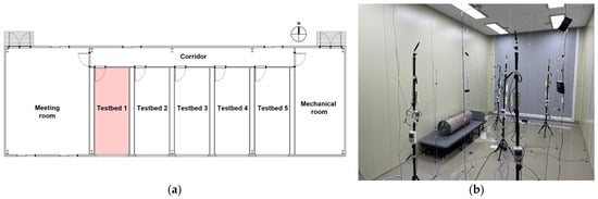
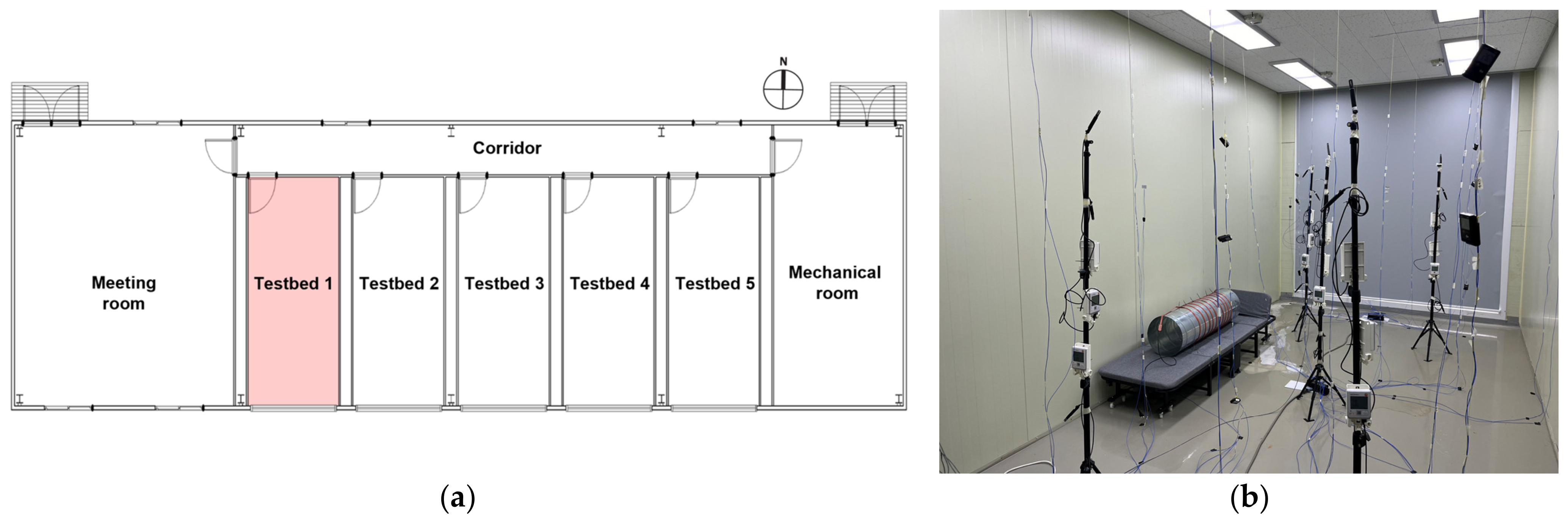
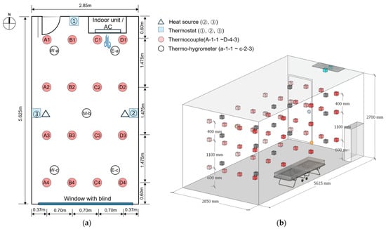
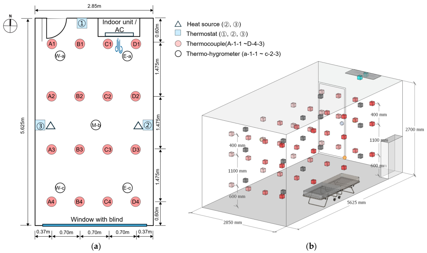
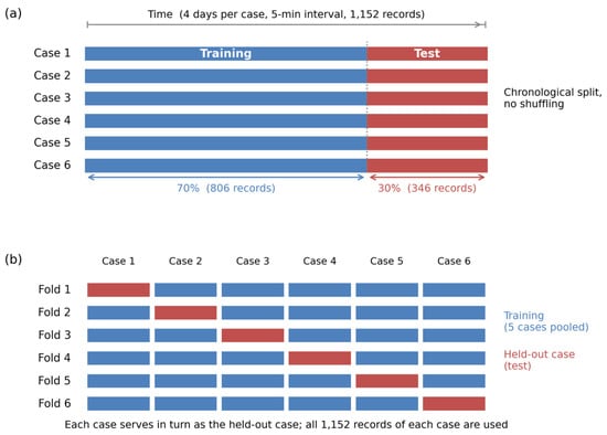
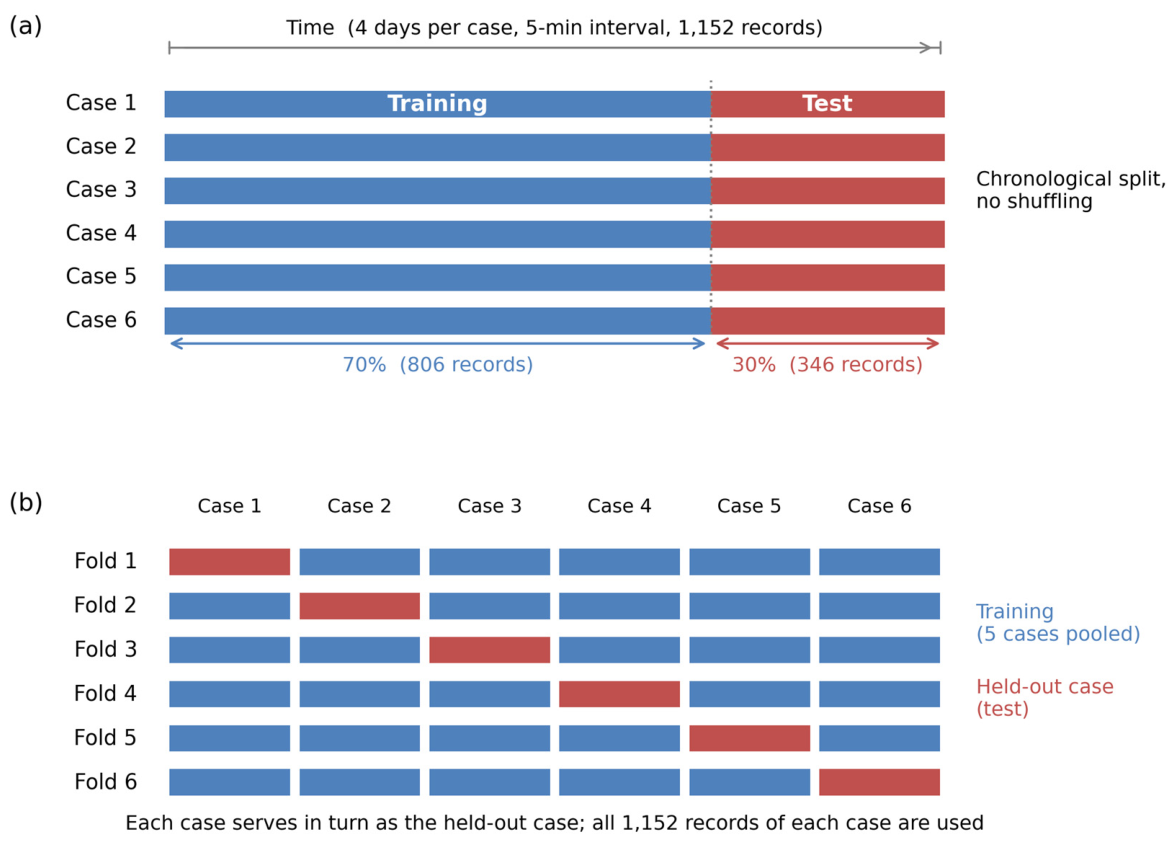
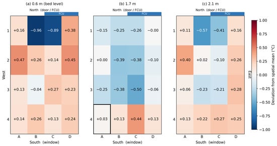
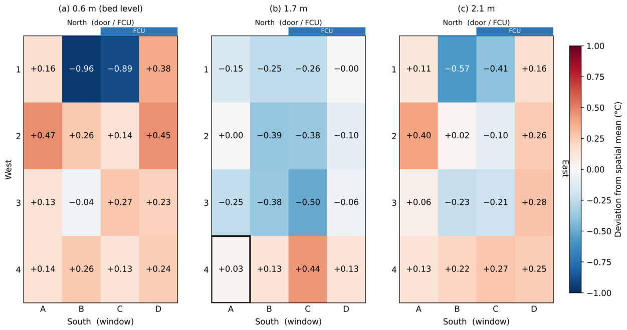
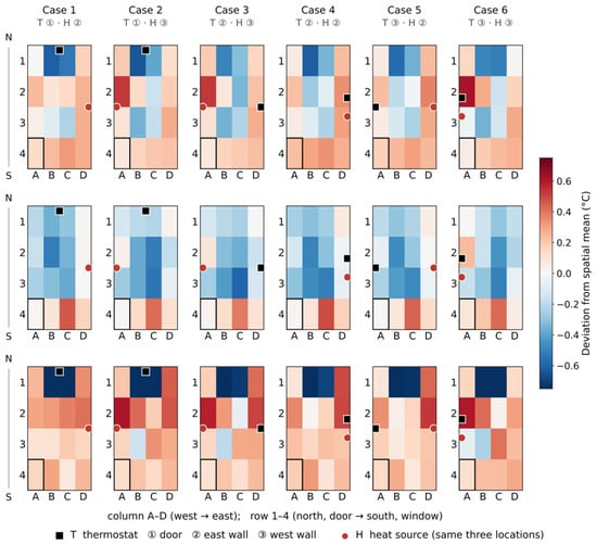
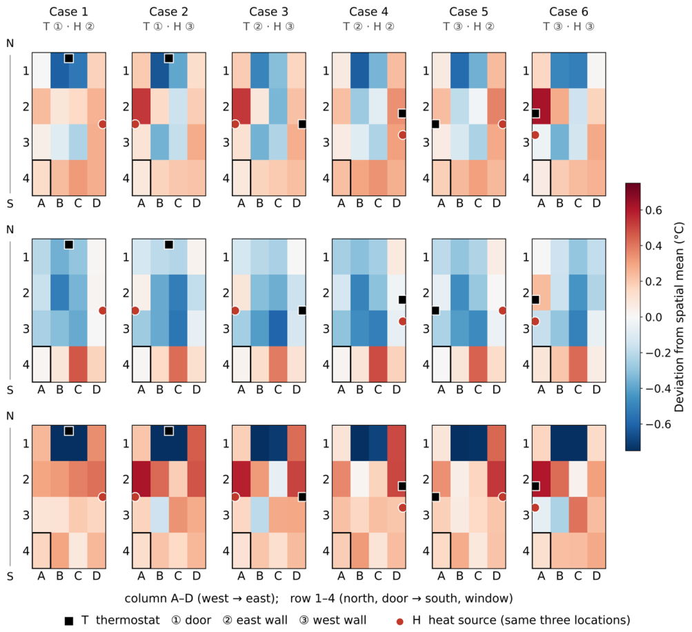
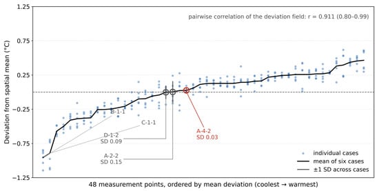
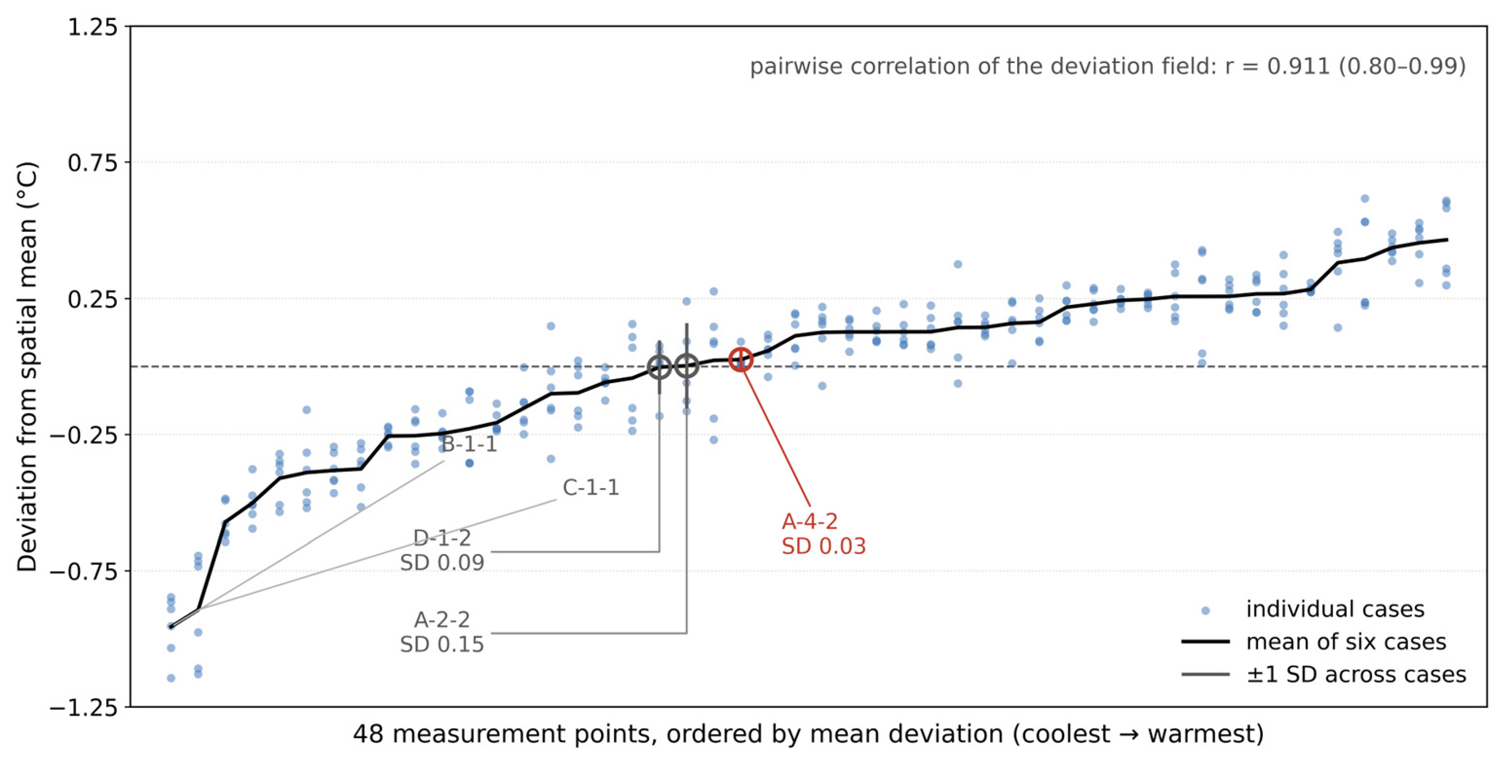
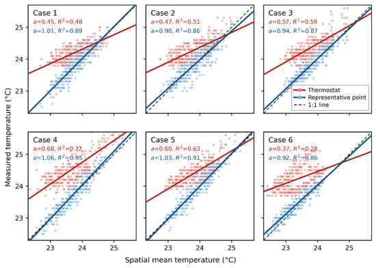
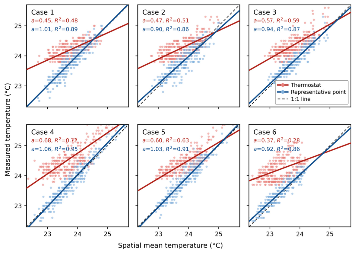
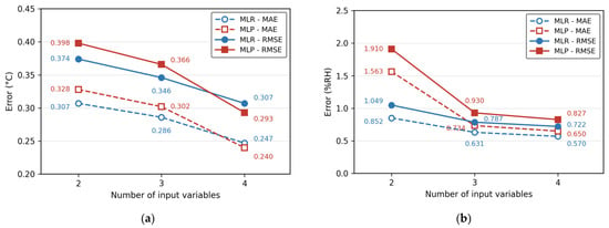
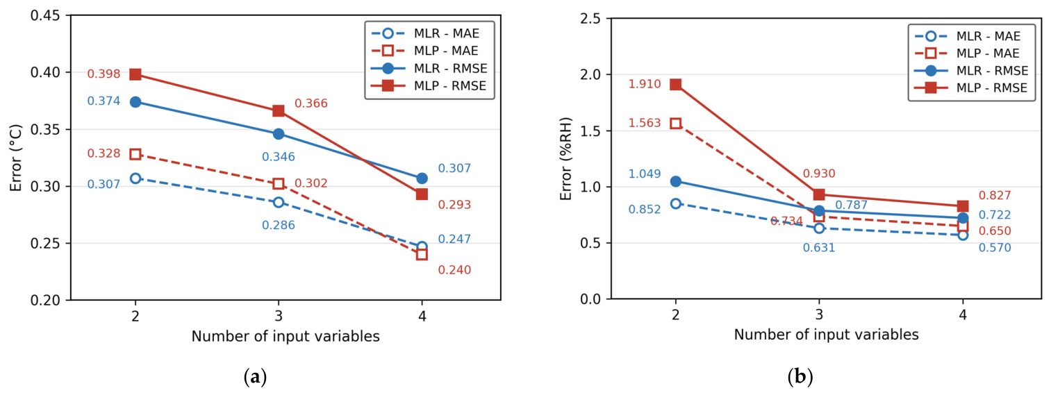
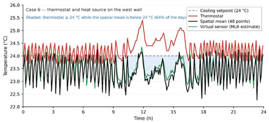
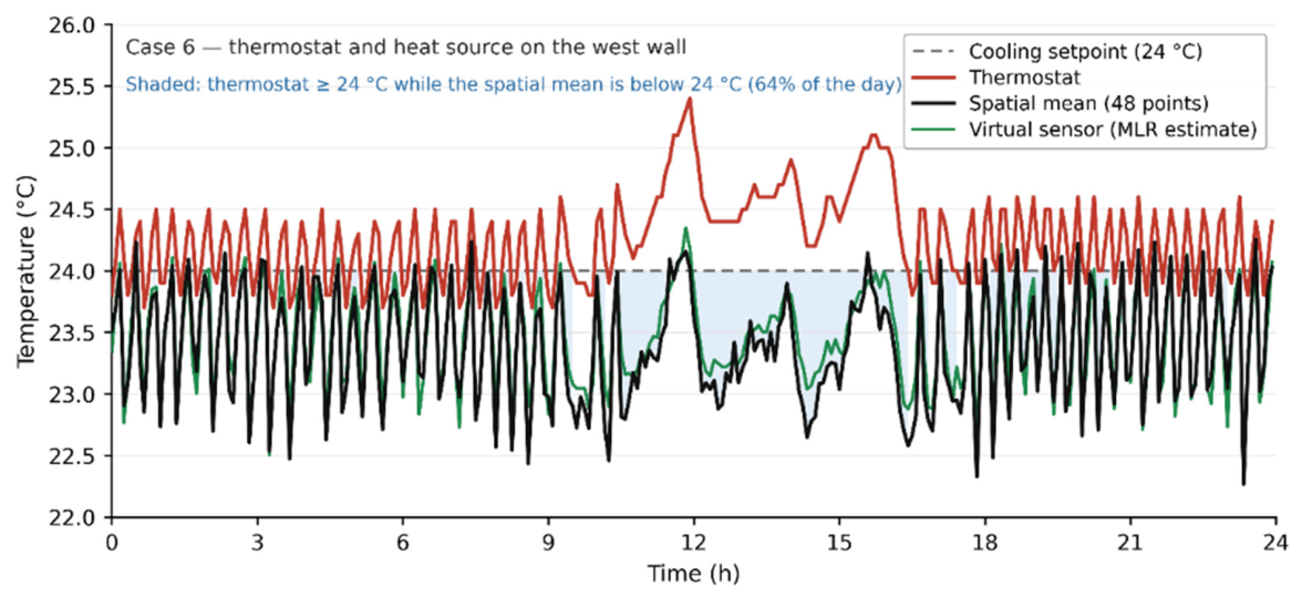

Disclaimer/Publisher’s Note: The statements, opinions and data contained in all publications are solely those of the individual author(s) and contributor(s) and not of MDPI and/or the editor(s). MDPI and/or the editor(s) disclaim responsibility for any injury to people or property resulting from any ideas, methods, instructions or products referred to in the content. |
© 2026 by the authors. Licensee MDPI, Basel, Switzerland. This article is an open access article distributed under the terms and conditions of the Creative Commons Attribution (CC BY) license.