Dynamic Response and Seismic Resilience of a Subway Station Subjected to Oblique SV-Wave Incidence

Abstract

To investigate the influence of oblique SV-wave incidence on the dynamic response and seismic resilience of subway stations, the viscoelastic artificial boundary combined with the equivalent nodal force method was used to implement the oblique SV-wave input, and a 3D soil-structure interaction finite element model was developed. The results indicate that when subjected to oblique SV-wave incidence at small angles, the subway station structure is dominated by shear deformation. Then, the rocking response gradually rises as the angle increases. At the near-critical-angle incidence, both the rocking angle and inter-story drift ratio increase sharply, resulting in exacerbated structural damage and a degradation of lateral stiffness. Time-history analyses were conducted using 11 ground-motion records, and seismic resilience was assessed through Monte Carlo simulation. Compared with vertical incidence, the results show that oblique incidence at the near-critical angle significantly degrades the structure’s seismic resilience. Its resilience rating drops significantly. Repair costs and repair time are much higher than the values at vertical incidence. The structure’s functional recoverability was substantially reduced. The rating for the casualty index decreased sharply, exposing serious safety hazards. These results indicate that resilience assessments derived from vertical incidence cause the seismic resilience of subway stations to be overestimated.

1. Introduction

Subway stations constitute critical nodes in urban lifeline systems. Their seismic resilience is essential to post-earthquake emergency response and functional recovery. During the 1995 Great Hanshin Earthquake, the Daikai subway station was severely damaged. This event drew widespread attention to the dynamic performance of shallow-buried, large-cross-section underground structures [1,2]. It also triggered a paradigm shift in seismic design—from “collapse prevention” towards “seismic resilience.” This concept emphasizes rapid post-earthquake functional recovery [3,4].

Incorporating the resilience concept into the seismic analysis of subway stations is a primary focus in current earthquake engineering research for underground structures [5,6,7,8]. The resilience concept was first proposed by Holling [9] in 1973 to describe a system’s capacity to sustain basic functions and autonomously recover following external disturbances; it has since been gradually extended to the fields of engineering and urban disaster prevention [10]. Bruneau et al. [11] were the first to propose a quantitative framework for assessing community seismic resilience, establishing a four-dimensional resilience measurement system—technical, organizational, social, and economic-centered on robustness, redundancy, resource allocability, and rapidity. Cimellaro et al. [12] subsequently introduced a functionality recovery function, quantifying resilience loss by the area bounded by the recovery curve and the time axis. Lin et al. [13] proposed a resilience assessment methodology for individual infrastructure systems based on engineering demand parameters and repair time. Ma et al. [7] established an index for the seismic resilience of underground frame structures based on two dimensions: resistance and recovery resilience. With the Daikai subway station serving as a case study, Yang et al. [14] concentrated on underground infrastructure types such as subway stations and established correction factors for repair time and economic loss that incorporate the inherent complexity characteristic of subterranean structures. Yang et al. [15] found that the triangular recovery function best matches the actual repair process at Daikai Station, and the exponential recovery strategy results in the smallest seismic resilience loss. In the field of structural seismic performance evaluation and optimization, studies on damage indices, modeling uncertainties, and multi-parameter assessment also provide essential support for resilience quantification. Wang et al. [16] focused on a mega frame–core tube–outrigger structural system and quantified the influence of modeling uncertainties on performance evaluation results under near-field and far-field earthquakes, providing a reference for uncertainty propagation studies in resilience analysis. Muhammad Shahzad et al. [17] compared the response differences in various steel plate shear wall systems under near-field ground motions, revealing the relative merits of different configurations from the perspective of damage characteristics. On this basis, Muhammad Shahzad et al. [18] performed a multi-parameter response control analysis on a novel mega substructure control system, and its optimization framework can serve as a reference for formulating resilience enhancement strategies. Accurate quantification of post-earthquake damage in underground structures and surrounding rock is essential for functional resilience assessment. While structural damage in earthquake engineering is typically characterized by macroscopic indicators such as inter-story drift ratio, recent advances in rock mechanics have demonstrated the potential of X-ray computed tomography (CT) combined with gray-level co-occurrence matrix (GLCM) texture features for non-destructive mesoscopic damage characterization. Xue et al. [19] established a CT-GLCM-based framework for quantifying mesoscopic damage in granite under cyclic liquid nitrogen shocks, proving more sensitive than conventional threshold segmentation. Li et al. [20] further revealed the microscale damage evolution and fracture propagation in thermally shocked granite using CT analysis, confirming the sensitivity of texture features for early damage detection.

The aforementioned resilience assessment methods all rest on the assumption of vertically incident bedrock ground motion; however, statistical studies indicate that in shallow-source earthquakes, seismic waves often arrive at the engineering site at an oblique angle, with body-wave incidence angles in near-field records reaching 20°~50° or even greater [21,22]. Under oblique incidence conditions, a spatially non-uniform motion field is generated at the ground surface, and the structure is subjected to pronounced traveling wave effects and asymmetric excitation; its dynamic response is often considerably more severe than that under vertical incidence [23,24].

For the accurate representation of structural response subjected to obliquely incident seismic waves, Lysmer and Kuhlemeyer [25] first proposed the viscous artificial boundary. Building on this work, Joyner and Chen [26] proposed the idea of equivalent nodal loads; they successfully resolved the challenge of introducing seismic waves into an elastic base by utilizing viscous boundary conditions and applying the associated equivalent loading. Deeks and Randolph [27] introduced spring elements to develop the viscoelastic artificial boundary. Liu et al. [28] subsequently established a three-dimensional time-domain viscoelastic artificial boundary and proposed an improved version that enhances the stability of explicit time integration, thereby providing a reliable approach for oblique seismic wave input. To address the wave problem in the outer domain, Zhao et al. [29] developed high-order accurate artificial boundary conditions. Huang et al. [30] further extended this approach to three-dimensional near-field wave problems. These high-order accurate artificial boundary conditions have since provided reliable methods for the input of obliquely incident seismic waves. Furthermore, Bao et al. [31] systematically investigated the stability behavior of the explicit algorithm within the framework of three-dimensional viscoelastic artificial boundary conditions, and further provided a theoretical basis for determining an appropriate time-step size.

Based on the viscoelastic artificial boundary and the equivalent nodal force method, oblique SV-wave input has been extensively adopted in the seismic response examination of underground structures. Wang X et al. [32] used SV and P waves with oblique incidence, conducted a parametric study on an underground powerhouse structure, and found that the most severe damage is observed under a 30°oblique incidence. The damage index increases significantly when rock-structure interaction is considered. They also systematically revealed the controlling effect of the interface contact state on dynamic stability, demonstrating that good contact can reduce seismic damage. Wang HY et al. [33] used oblique incidence SV-waves as input and conducted an incremental dynamic analysis (IDA) study on a utility tunnel in a horizontally inhomogeneous site. The failure probability was found to grow as the incident angle and PGA increase, especially in cases where the angle reaches 30° and the PGA surpasses 0.6 g, at which point the severe damage and collapse probabilities experience a substantial rise. Zhu et al. [34] systematically revealed the non-uniform loading characteristics induced by oblique incidence: at small oblique angles, the observation station is primarily subjected to lateral shear deformation; whereas at large angles, it transitions to predominantly vertical shear deformation; moreover, under oblique seismic wave incidence, the station exhibits a markedly enhanced vertical acceleration response. Wang Y et al. [35], using Daikai Station as a case study, demonstrated that at the critical angle, displacement, internal forces, and stresses all reach their peak values. Whereas the response substantially attenuates once the critical angle is exceeded. Zhao et al. [36] conducted an investigation into the seismic response and damage progression of integrated above-ground-underground structures under obliquely incident SV waves. As the incidence angle grows, the progression of damage in underground structural beam members during the elastoplastic phase is demonstrated. Qiu et al. [37] demonstrated that large-scale underground frame structures exhibit distinctive response patterns and failure modes under oblique SV-wave incidence. Xiong et al. [38] found that under an obliquely incident SV-wave with spatial variation, soil nonlinearity significantly amplifies the rocking and torsional responses of the foundation and superstructure. This amplification effect is jointly controlled by the incidence angle and soil nonlinearity. Therefore, seismic damage assessment must simultaneously consider these two factors.

Collectively, these studies indicate that oblique SV-wave incidence substantially amplifies seismic responses in underground structures while simultaneously modifying failure mechanisms. However, existing seismic resilience assessments of subway stations have been based on the assumption of vertical incidence. The non-uniform excitation induced by oblique incidence and the critical-angle amplification effect can greatly affect resilience indices. To address this issue, a 3D finite element model accounting for soil-structure interaction is developed. A viscoelastic artificial boundary combined with the equivalent nodal force method is also adopted to input oblique SV waves at various incident angles. Based on this, the study systematically analyzes how the incidence angle affects the station’s dynamic response and seismic resilience indices.

2. Seismic Input Methodology and Finite Element Modeling

2.1. Viscoelastic Artificial Boundary and Equivalent Nodal Forces

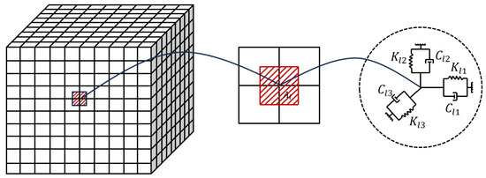
Viscoelastic artificial boundaries are realized by placing springs and dampers at the boundary nodes, which simultaneously absorb scattered wave energy and provide low-frequency elastic recovery stiffness. This effectively improves computational accuracy and stability and facilitates integration with general-purpose finite element programs, as illustrated in Figure 1. The normal and tangential spring stiffness and damping coefficients are given by [34]:

$$K_N=A_L\cdot {\displaystyle \frac{1}{1+A}}\cdot {\displaystyle \frac{\lambda +2G}{R}}, C_n=A_{L}B\rho c_p$$

(1)

$$K_T=A_L\cdot {\displaystyle \frac{1}{1+A}}\cdot {\displaystyle \frac{G}{R}}, C_t=A_{L}B\rho c_s$$

(2)

where $K_N$ and $K_T$ denote the stiffness coefficients of the artificial boundary in the normal and tangential directions, respectively; $C_n$ and $C_t$ represent the damping coefficients of the artificial boundary in the normal and tangential directions, respectively; A is the correction coefficient for spring stiffness, taken as 0.8; B is the correction coefficient for damping, taken as 1.1 [39]; $A_L$ is the effective influence area of the boundary node on the artificial boundary, as shown in Figure 1; $\lambda$ is the first Lamé constant of the soil; G defines the soil shear modulus.; $c_s$ is the S-wave velocity; $c_p$ is the P-wave velocity; $\rho$ defines the soil mass density; and R represents the distance from the wave source to the artificial boundary.

Figure 1. Illustration of the three-dimensional viscoelastic boundary.

From Snell’s law, when an SV wave is incident on a free ground surface at an angle $\alpha$, the critical angle ${\alpha }_{\mathrm{c}\mathrm{r}}$ satisfies:

$${\alpha }_{\mathrm{c}\mathrm{r}}=\arcsin \left({\displaystyle \frac{c_s}{c_p}}\right)$$

(3)

where $\nu$ is the soil Poisson’s ratio. In this study, $\nu =0.4$ and the critical angle is ${\alpha }_{cr}\approx {24.09}^{\circ }$.

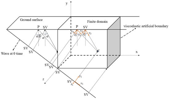
This study adopts the computational method proposed in Ref. [38] and extends it to the three-dimensional case to calculate the equivalent nodal forces induced by oblique incident SV waves. Figure 2 schematically illustrates SV-wave oblique incidence on a horizontal ground surface, where $\beta$ is the P-wave reflection angle, given by Snell’s law as: $\beta =arcsin(c_p sin\alpha /c_s)$. The displacement at node $l$ ($x_l$, $y_l$ $z_l$) can be decomposed into components from the incident SV-wave, reflected SV-wave, and reflected P-wave. The local coordinate systems ($x_i$, $y_i$ $z_i$) ($i$ = 1, 2, 3) are defined.

Figure 2. Schematic illustration of 3D plane SV-wave oblique incidence.

When an SV wave reaches a free surface, it generates a reflected SV wave and a reflected P wave; the corresponding reflection amplitude ratios are denoted as A₁ and A₂, respectively:

$$A_1={\displaystyle \frac{c_s^2\mathrm{s}\mathrm{i}\mathrm{n} 2\alpha \mathrm{s}\mathrm{i}\mathrm{n} 2\beta -c_p^2{\mathrm{c}\mathrm{o}\mathrm{s}}^2 2\alpha }{c_s^2\mathrm{s}\mathrm{i}\mathrm{n} 2\alpha \mathrm{s}\mathrm{i}\mathrm{n} 2\beta +c_p^2{\mathrm{c}\mathrm{o}\mathrm{s}}^2 2\alpha }}$$

(4)

$$A_2={\displaystyle \frac{2c_s{c}_p\mathrm{s}\mathrm{i}\mathrm{n} 2\alpha \mathrm{c}\mathrm{o}\mathrm{s} 2\alpha }{c_s^2\mathrm{s}\mathrm{i}\mathrm{n} 2\alpha \mathrm{s}\mathrm{i}\mathrm{n} 2\beta +c_p^2{\mathrm{c}\mathrm{o}\mathrm{s} }^{2}2\alpha }}$$

(5)

where $A_1$ is the ratio of the displacement amplitude of the reflected SV wave to that of the incident SV wave, and $A_2$ is the ratio of the displacement amplitude of the reflected P wave to that of the incident SV wave.

Then, the displacement transformation matrices from the local coordinate system to the global coordinate system for the incident SV wave, reflected SV wave and reflected P wave are as follows:

$$\text{incident SV-wave}:T_1=\left[\begin{array}{ccc}cos\alpha & -sin\alpha & 0\\ sin\alpha & cos\alpha & 0\\ 0& 0& 1\end{array}\right]$$

(6)

$$\text{reflected SV-wave}:T_2=\left[\begin{array}{ccc}-cos\alpha & -sin\alpha & 0\\ sin\alpha & -cos\alpha & 0\\ 0& 0& 1\end{array}\right]$$

(7)

$$\text{reflected P-wave}:T_3=\left[\begin{array}{ccc}-cos\beta & -sin\beta & 0\\ sin\beta & -cos\beta & 0\\ 0& 0& 1\end{array}\right]$$

(8)

In the global coordinate system, the free-field displacement component at the artificial boundary node $l$ is as follows:

$$U={\displaystyle \sum _{n=1}^3} T_n^T{U}_n,\dot{U}={\displaystyle \sum _{n=1}^3} T_n^T{\dot{U}}_n$$

(9)

$$U_1={\left[\begin{array}{ccc}{u}_{is}(t-{∆t}_1)& 0& 0\end{array}\right]}^T$$

(10)

$$U_2={\left[\begin{array}{ccc}{A}_1{u}_{rs}(t-{∆t}_2)& 0& 0\end{array}\right]}^T$$

(11)

$$U_3={\left[\begin{array}{ccc}0& A_2{u}_{rp}(t-{∆t}_3)& 0\end{array}\right]}^T$$

(12)

where the $u_{is}$ denotes the displacement of the incident SV-wave; $u_{rs}$ denotes the displacement of the reflected SV-wave; $u_{rp}$ denotes the displacement of the reflected P-wave.

The time differences in the incident SV-wave, reflected SV-wave, and reflected P-wave arriving at the boundary node $l$ are ${∆t}_1$, ${∆t}_2$, and ${∆t}_3$, respectively:

$${∆t}_1={\displaystyle \frac{x_{l}sin\alpha +y_{l}cos\alpha }{c_s}}$$

(13)

$${∆t}_2={\displaystyle \frac{x_{l}sin\alpha +(2H-y_l)cos\alpha }{c_s}}$$

(14)

$${∆t}_3={\displaystyle \frac{x_{l}sin\alpha +Hcos\alpha +(y_l-H)tan\beta sin\alpha }{c_s}}+{\displaystyle \frac{H-y_l}{c_{p}cos\beta }}$$

(15)

where $H$ is the height of the finite domain.

In the local coordinate system, the incoming stress at the boundary node, resulting from the superposition of the incident SV-wave, reflected SV-wave, and reflected P-wave, is as follows:

$${\sigma }_{li}^1=\left[\begin{array}{ccc}0& {\tau }_{xy}^1& 0\\ {\tau }_{xy}^1& 0& 0\\ 0& 0& 0\end{array}\right],{\tau }_{xy}^1=-{\displaystyle \frac{G}{c_s}}{\dot{u}}_{is}(t-{∆t}_1)$$

(16)

$${\sigma }_{li}^2=\left[\begin{array}{ccc}0& {\tau }_{xy}^2& 0\\ {\tau }_{xy}^2& 0& 0\\ 0& 0& 0\end{array}\right],{\tau }_{xy}^2=-{\displaystyle \frac{G}{c_s}}{A_1\dot{u}}_{is}(t-{∆t}_2)$$

(17)

$$\begin{gathered} {\sigma }_{li}^3=\left[\begin{array}{ccc}{\sigma }_{xx}^3& 0& 0\\ 0& {\sigma }_{yy}^3& 0\\ 0& 0& {\sigma }_{zz}^3\end{array}\right], \\ {\sigma }_{xx}^3={\sigma }_{zz}^3=-{\displaystyle \frac{\lambda }{c_P}}{A_2\dot{u}}_{is}\left(t-{∆t}_3\right),{\sigma }_{yy}^3=-{\displaystyle \frac{\lambda +2G}{c_P}}{A_2\dot{u}}_{is}\left(t-{∆t}_3\right) \end{gathered}$$

(18)

In the global coordinate system, the stress matrix at node $l$ is as follows:

$$\mathsf{\sigma }={\displaystyle \sum _{n=1}^3} T_n^T{\sigma }^n{T}_n$$

(19)

2.2. Verification of the Oblique-Wave Input Implementation

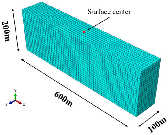
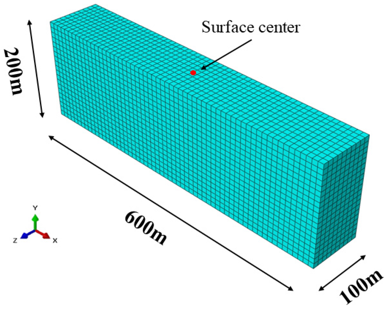
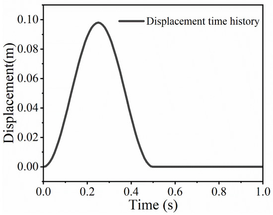
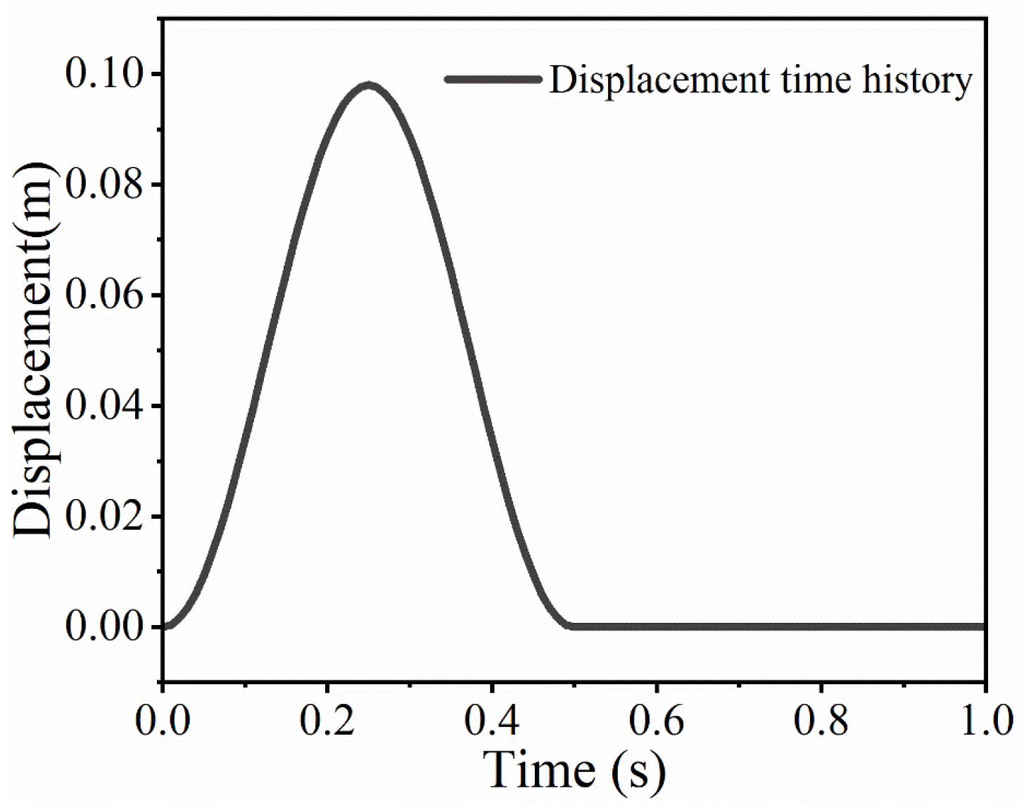
To validate the accuracy of the oblique-incidence seismic wave input method developed in this paper, a test model was constructed, as shown in Figure 3. The mass density of the soil is 2000 kg/m³, the elastic modulus is 1 GPa, and the Poisson’s ratio is 0.3. The test model is a rectangular prism measuring 600 m × 200 m × 100 m, meshed into cubes with a side length of 10 m. Figure 4 shows the incident SV-wave displacement time history. Equation (20) is the formula for the input pulse.

$$f\left(t\right)=16A_0\left[L\left({\displaystyle \frac{t}{t_0}}\right)-4L\left({\displaystyle \frac{t}{t_0}}-{\displaystyle \frac{1}{4}}\right)+6L\left({\displaystyle \frac{t}{t_0}}-{\displaystyle \frac{1}{2}}\right)\right]-4L\left({\displaystyle \frac{t}{t_0}}-{\displaystyle \frac{3}{4}}\right)+L\left({\displaystyle \frac{t}{t_0}}-1\right)$$

(20)

where $L\left(x\right)={\left(x\right)}^{3}H\left(x\right)$, $H\left(x\right)$ represents the Heaviside function.

Figure 3. Finite element case study model.

Figure 4. Incident SV wave displacement time histories.

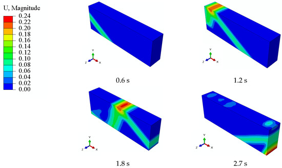
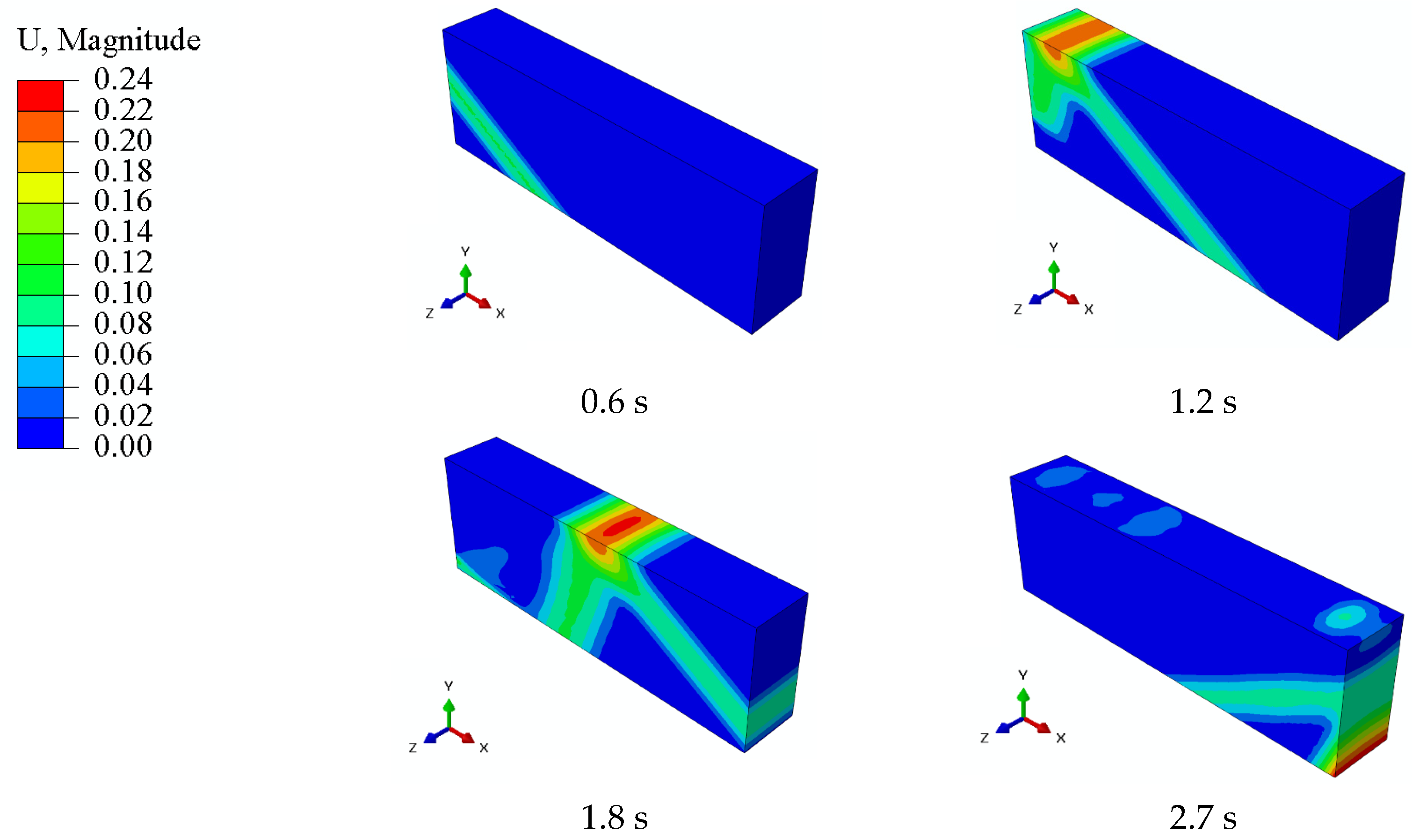
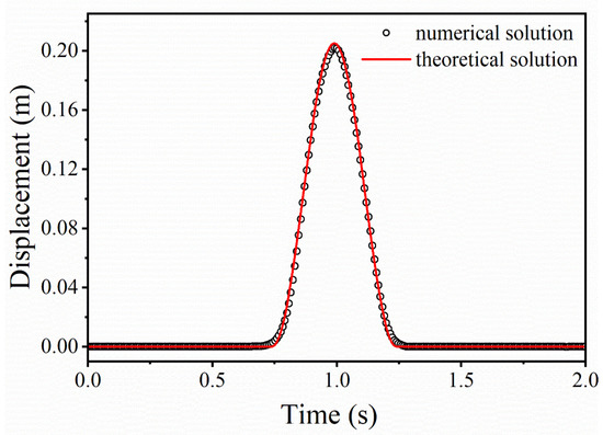
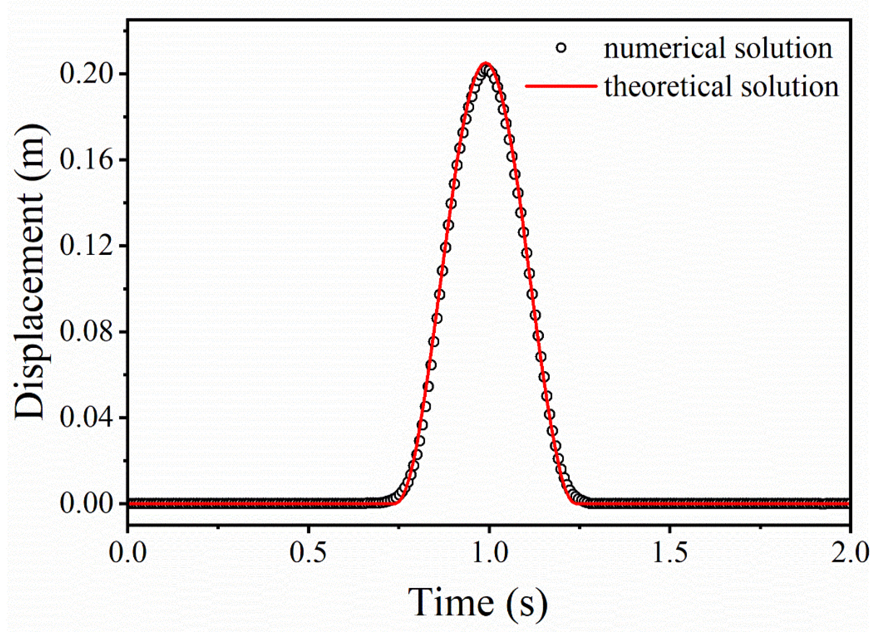
At 15° incidence, the displacement field contour plot is shown in Figure 5. It clearly shows the wavefronts of the incident SV wave, the reflected SV wave, and the reflected P wave, indicating that the propagation of the SV wave in homogeneous soil has been successfully simulated. Figure 6 compares the numerical and theoretical solutions in the x-direction at the center point of the soil surface. The good agreement between the two solutions verifies the validity of the adopted SV-wave input method.

Figure 5. Displacement-field contours for the obliquely incident SV wave.

Figure 6. Numerical and analytical x-direction displacement time histories at the free-field surface midpoint.

2.3. Numerical Model of Soil–Structure Interaction

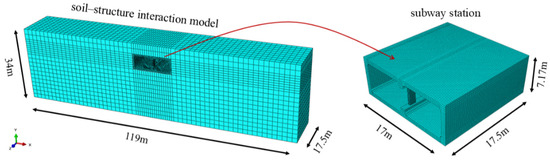
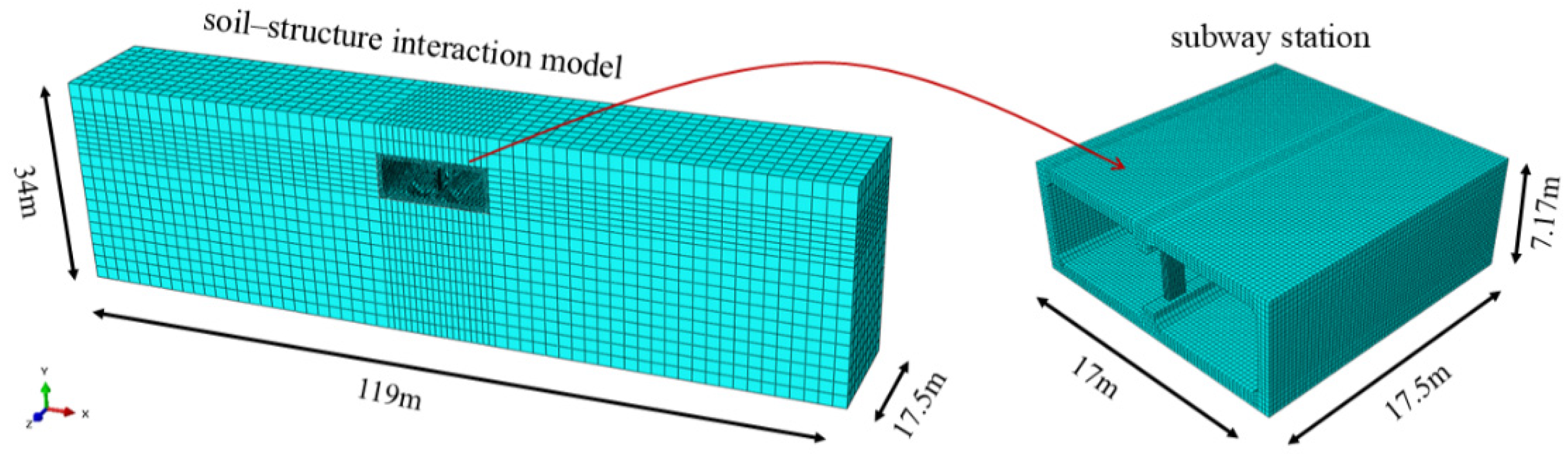
To accurately simulate the dynamic response of the soil-station at obliquely incident SV waves, this paper uses ABAQUS 2024 software to develop a 3D solid finite element model based on the Daikai station, with the station dimensions set at 17 m × 17.5 m × 7.17 m. The oblique-incidence SV wave input method used in this paper is derived based on a homogeneous elastic medium; therefore, the model also assumes a homogeneous soil, ensuring strict consistency between the method and the model. According to Section 6.9.1 of the code for seismic design of urban rail transit structures (GB 50909–2014) [40], to minimize reflections generated at the model boundaries during time-history analysis, the lateral boundaries are set to be no less than three times the structural width, and the distance from the bottom boundary to the base of the station is no less than three times the structural height. Therefore, the final dimensions of the soil mass were determined to be 119 m × 17.5 m × 34 m, as illustrated in Figure 7.

Figure 7. Subway station model.

Both the station structure and the soil were discretized with C3D8R hexahedral elements, whereas T3D2 truss elements represented the reinforcing bars. The mesh was locally refined in the column. The mesh discretization followed the wave propagation criterion proposed by Kuhlemeyer and Lysmer [41], which recommends that the element dimensions are restricted to no more than 1/8 to 1/10 of the wavelength corresponding to the maximum significant frequency of the input ground motions. The station model was meshed at 0.25 m, with the mesh refined to 0.1 m at the central columns, resulting in 56,240 elements. The reinforcement was modeled using a characteristic mesh size of 0.2 m, consisting of 40,076 elements. A 2 m mesh was employed to discretize the soil domain, with local refinement to 1 m near the soil–structure interface, resulting in 11,466 elements.

To accurately simulate the complex stress state of the station under oblique seismic wave incidence, the Concrete Damaged Plasticity (CDP) constitutive model was utilized.

Table 1 lists the CDP parameters, which were adopted from the values used by Jia [42]. The steel rebars are simulated via a bilinear stress–strain model, and an “Embedded” constraint was employed to incorporate them into the surrounding concrete. A “Surface-to-Surface” contact was adopted to define the contact interaction between the station and soil. Normal interaction was defined via a “Hard” contact law, whereas tangential interaction followed a penalty formulation with a friction coefficient of 0.4. The mechanical parameters of concrete, reinforcing steel, and soil are summarized in Table 2.

Table 1. CDP parameters.

Dilation Angle	Eccentricity	fb0/fc0	K	Viscosity Parameter
30°	0.1	1.16	0.6667	0.05

Where f_b0/f_c0 is the ratio of the biaxial compressive strength to the uniaxial compressive strength; K is the shape factor of the yield surface.

Table 2. Concrete, reinforcing steel, and soil material properties.

Material	C40 Concrete	Reinforcing Steel	Soil
Density	2500 kg/m3	7850 kg/m3	1900 kg/m3
Poisson’s Ratio	0.2	0.3	0.4
Modulus of Elasticity	32,500 MPa	200,000 MPa	192 MPa
Tensile strength	2.39 MPa	—	—
Compressive strength	26.8 MPa	—	—
Yield Strength	—	400 MPa	—
Ultimate Strength	—	540 MPa	—
Rayleigh damping	α: 0.492835	—	—
	β: 0.004398

“—” means that this parameter is not used in the material settings in Abaqus.

3. Dynamic Response of the Station Under Oblique SV Waves

3.1. Analysis Framework and Seismic Input

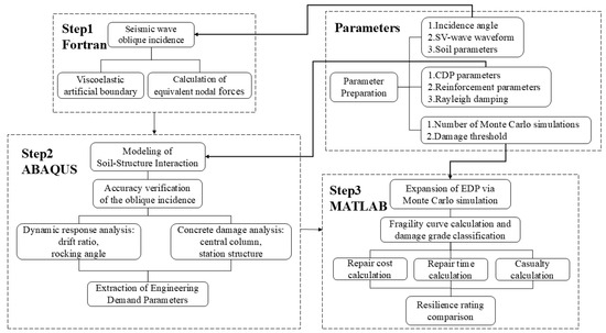
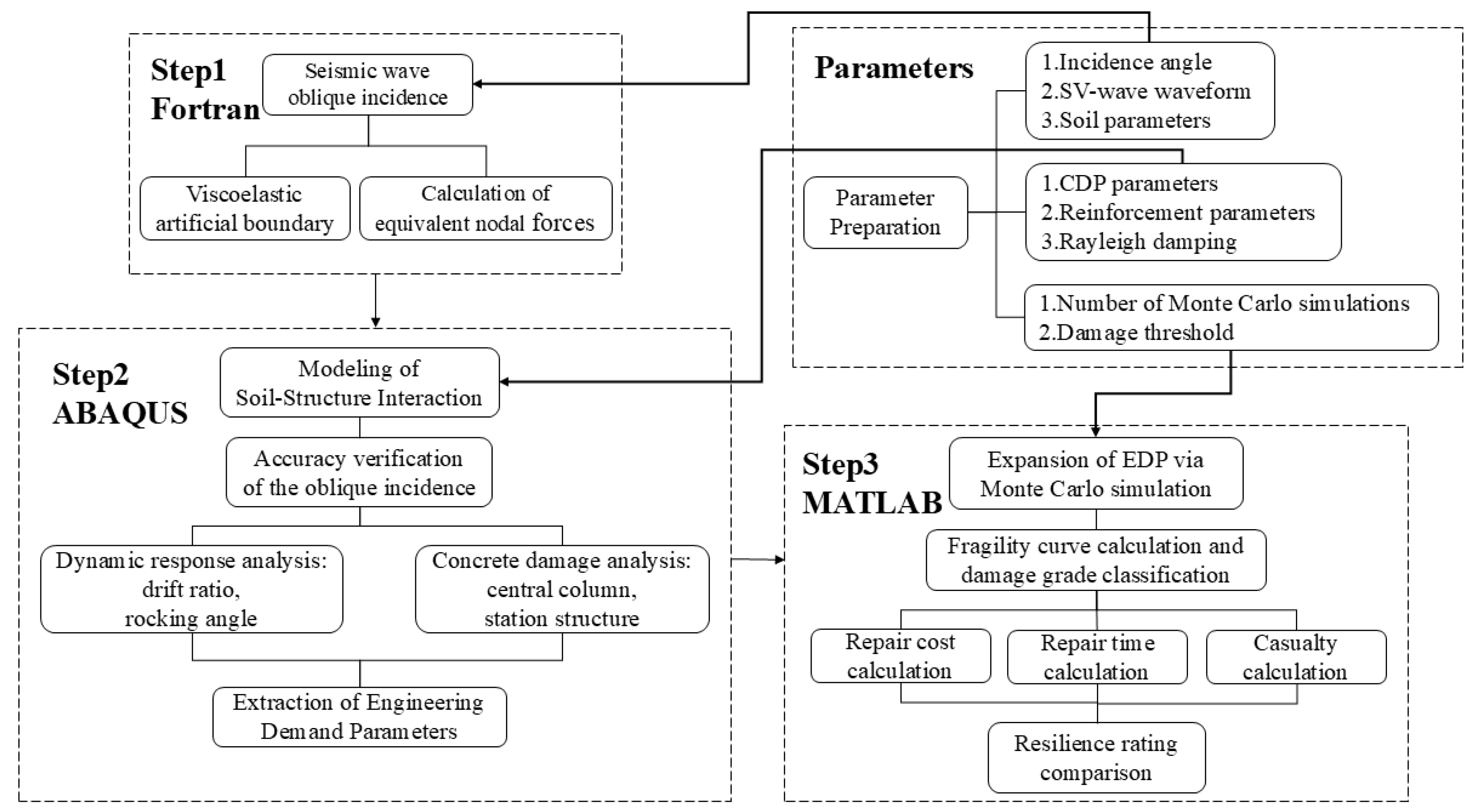
This paper develops a framework for implementing the oblique incidence input of SV waves and assessing seismic resilience, as illustrated in Figure 8. First, the parameters of the viscoelastic artificial boundary and the equivalent nodal forces are calculated using Fortran. Then, the above boundary conditions and loads were implemented in ABAQUS 2024 to simulate an obliquely incident SV wave, and the validity of the adopted input method was verified. The explicit dynamic method is adopted. Dynamic time-history analyses of the station are performed by varying the oblique incidence angle, and the structural engineering demand parameters (EDPs) are obtained. A program written in MATLAB R2020b was then used to augment the sample size of the EDPs via Monte Carlo simulation. Based on the augmented data, damage-state exceedance probabilities conditional on EDP are developed. From these curves, damage states are classified, and various resilience indices are calculated, thus completing the seismic resilience rating.

Figure 8. Computational and seismic resilience assessment workflow for obliquely incident SV waves.

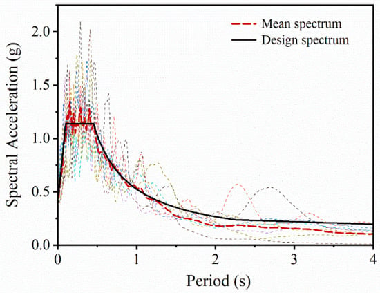
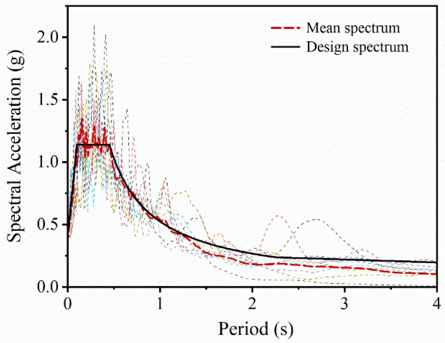
In accordance with the Code for Seismic Design of Buildings (GB 50011–2010) [43] and the Standard for Seismic Resilience Assessment of Buildings (GB/T 38591–2020) [44], seismic resilience assessment by means of time-history analysis requires a minimum of 11 sets of seismic motion records. Both recorded and artificial acceleration time histories were included. On the basis of the natural frequency of the structure, the Pacific Earthquake Engineering Research Center (PEER) strong-motion database served as the source for the selection of eight recorded ground motions. The code-specified design response spectrum served as the basis for generating three artificial records in MATLAB. All ground motion records were uniformly scaled to a peak ground acceleration (PGA) of 0.4 g and 0.2 g, representing the rare earthquake and the design basis earthquake, respectively. In total, 11 input ground motion sets were obtained. To ensure that the ground motion records are compatible with the site characteristics, the acceleration response spectra were compared with the target response spectrum specified in the seismic design code. As shown in Figure 9, the mean response spectrum closely matches the target spectrum specified in the code.

Figure 9. Selected seismic wave response spectra and target spectrum.

From the 11 ground motion records selected above, a single record was selected to systematically examine how the structural dynamic response is influenced by the oblique incidence angle. This record was selected because its dominant frequency is close to the fundamental natural frequency of the station.

This proximity results in a near-resonance condition that amplifies the structural response and facilitates a more systematic evaluation of the influence of the incident angle. The 15 s duration is moderate, allowing stable excitation of the nonlinear structural response while avoiding excessive cumulative damage that may obscure the intrinsic influence of the incident angle.

It should be noted that strictly adopting the theoretical critical angle of α = 24.09° may induce numerical instability in the equivalent loads and displacement fields at artificial boundaries, thereby affecting computational accuracy. Therefore, the maximum angle is set to α = 24°. To accurately capture the variation in structural response near the critical angle, a refined set of cases was considered within the range of α = 23°~24°. Table 3 lists the considered analysis cases.

Table 3. Configuration of Response Analysis Cases.

Seismic Ground Motion	Case Number	Incident Angle $\mathit{\alpha }$
Artificial 1 (PGA = 0.4 g)	1	0°
	2	5°
	3	10°
	4	15°
	5	20°
	6	23°
	7	23.25°
	8	23.50°
	9	23.75°
	10	24°

These settings enable systematic analysis of the structural response as the incidence angle increases from vertical to the near-critical angle, and accurate capture of the corresponding response characteristics.

3.2. Inter-Story Drift Ratio and Rocking Angle Analysis

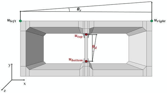
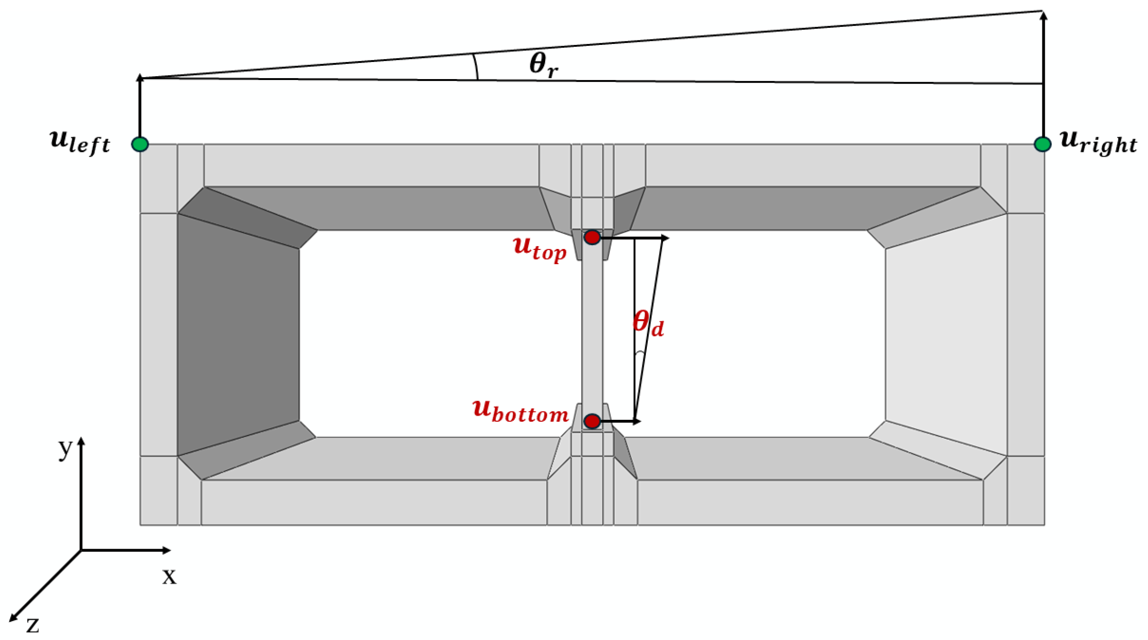
To quantitatively characterize the station rocking response under obliquely incident SV-wave excitation, the overall structural rocking angle ${\theta }_{\mathrm{r}}$ is defined as shown in Figure 10:

$${\theta }_{\mathrm{r}}={\displaystyle \frac{u_{\mathrm{r}\mathrm{i}\mathrm{g}\mathrm{h}\mathrm{t}}\left(t\right)-u_{\mathrm{l}\mathrm{e}\mathrm{f}\mathrm{t}}\left(t\right)}{B}}$$

(21)

where $u_{\mathrm{r}\mathrm{i}\mathrm{g}\mathrm{h}\mathrm{t}}\left(t\right)$ and $u_{\mathrm{l}\mathrm{e}\mathrm{f}\mathrm{t}}\left(t\right)$ denote the vertical displacements at the right and left points of the two sidewalls; $B$ is the length of the station.

Figure 10. Schematic diagram of ${\theta }_{\mathrm{r}}$ and ${\theta }_{\mathrm{d}}.$

The inter-story drift ratio ${\theta }_{\mathrm{d}}$, follows the standard seismic code definition as shown in Figure 10:

$${\theta }_{\mathrm{d}}={\displaystyle \frac{u_{\mathrm{t}\mathrm{o}\mathrm{p}}\left(t\right)-u_{\mathrm{b}\mathrm{o}\mathrm{t}\mathrm{t}\mathrm{o}\mathrm{m}}\left(t\right)}{H}}$$

(22)

where $u_{\mathrm{t}\mathrm{o}\mathrm{p}}\left(t\right)$ and $u_{\mathrm{b}\mathrm{o}\mathrm{t}\mathrm{t}\mathrm{o}\mathrm{m}}\left(t\right)$ are the horizontal displacements at the top and bottom nodes of the central column; H is the clear height of the column.

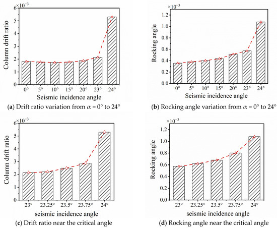
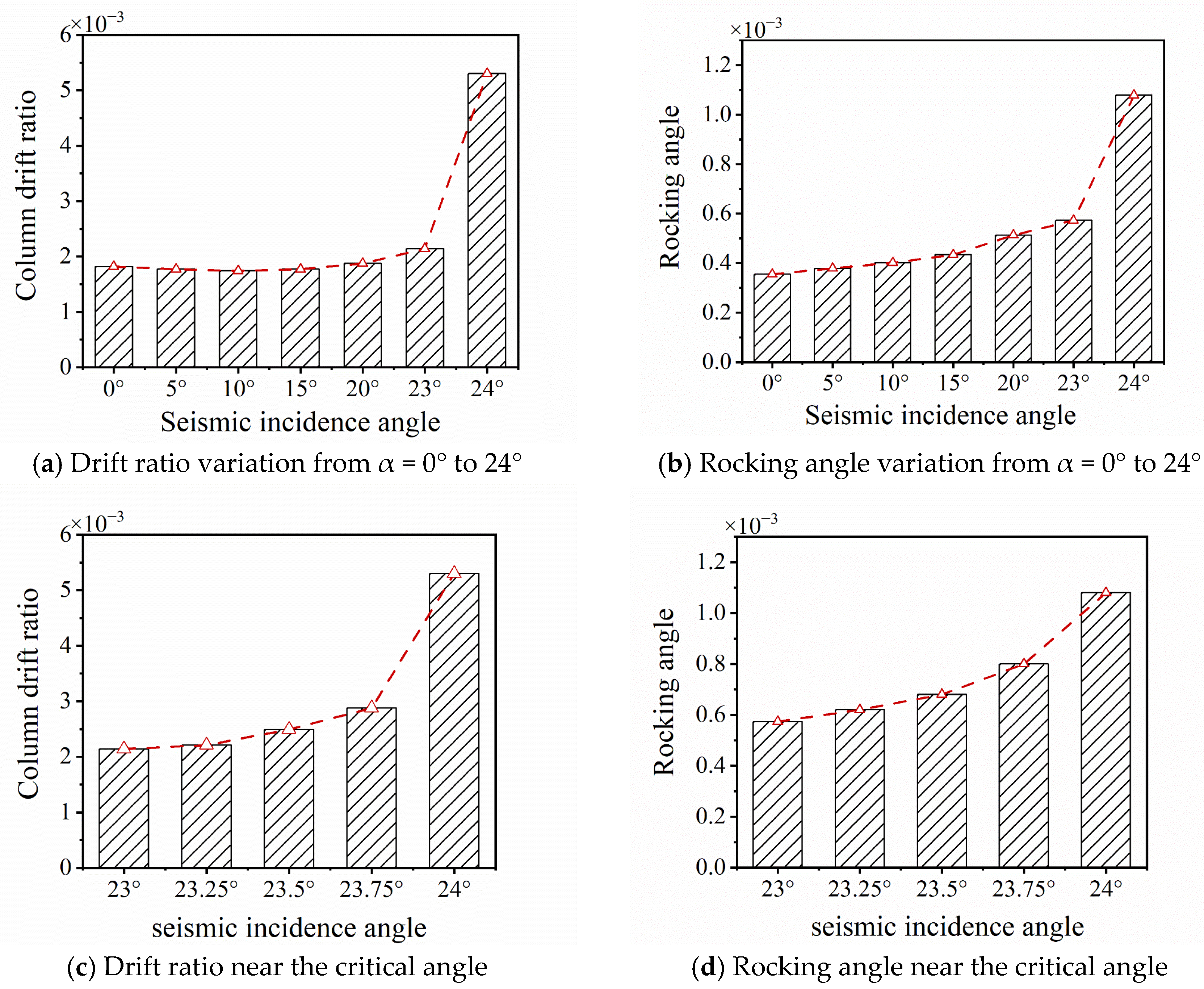
To investigate the response of the central column subjected to obliquely incident SV waves, the variations of ${\theta }_{\mathrm{d}}$ and ${\theta }_{\mathrm{r}}$ with incidence angle are first analyzed in Figure 11a,b.

Figure 11. Variation in the inter-story drift ratio and rocking angle with SV-wave incidence angle.

For $\alpha$ from 0° to 10°, the ${\theta }_{\mathrm{d}}$ decreases slightly as the incident angle increases, reaching a minimum near $\alpha$ = 10°; subsequently, it continues to increase in the range of α from 10° to 23°; When $\alpha$ reaches the near-critical angle of 24°, the ${\theta }_{\mathrm{d}}$ increases sharply. The response of the ${\theta }_{\mathrm{r}}$ exhibits a two-stage characteristic: in the 0–23° range of $\alpha$, the ${\theta }_{\mathrm{r}}$ increases slowly; in the 23–24° range of $\alpha$, the rate of increase becomes more pronounced, and as $\alpha$ approaches 24°, the amplitude of the ${\theta }_{\mathrm{r}}$ approximately doubles compared with that at $\alpha$ = 23°.

The aforementioned response variation patterns are governed by the combined effects of horizontal shear deformation and rocking response. Shear deformation directly induces relative horizontal displacement at the column ends, with its magnitude primarily governed by the horizontal component of ground motion. In contrast, the rocking response causes global structural tilting and additional column end rotation, thereby increasing the ${\theta }_{\mathrm{d}}$. For $\alpha$ from 0° to 10°, the traveling-wave effect is not significant, and the increase in the ${\theta }_{\mathrm{r}}$ is relatively small, indicating that the structural response remains dominated by horizontal shear deformation. Meanwhile, the horizontal SV-wave component decreases progressively with the rise in the incidence angle, resulting in a reduction in ${\theta }_{\mathrm{d}}$. In the 10°~23° range of $\alpha$, the traveling-wave effect gradually rises, leading to an increase in ${\theta }_{\mathrm{r}}$. Meanwhile, ${\theta }_{\mathrm{d}}$ also begins to increase, indicating a transition toward a shear-rocking composite response.

A more detailed analysis was performed in the 23°~24° range of $\alpha$, as shown in Figure 11c,d. Both ${\theta }_{\mathrm{d}}$ and ${\theta }_{\mathrm{r}}$ increase rapidly and reach their maximum at $\alpha$ = 24°, indicating a pronounced sensitivity of the structural response to variations in the incident angle within this range. Near the critical incidence angle, even small variations in the incidence angle can induce significant changes in the structural response.

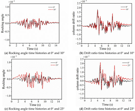
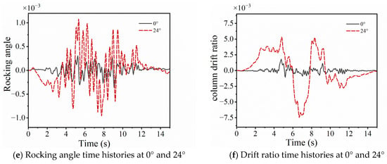
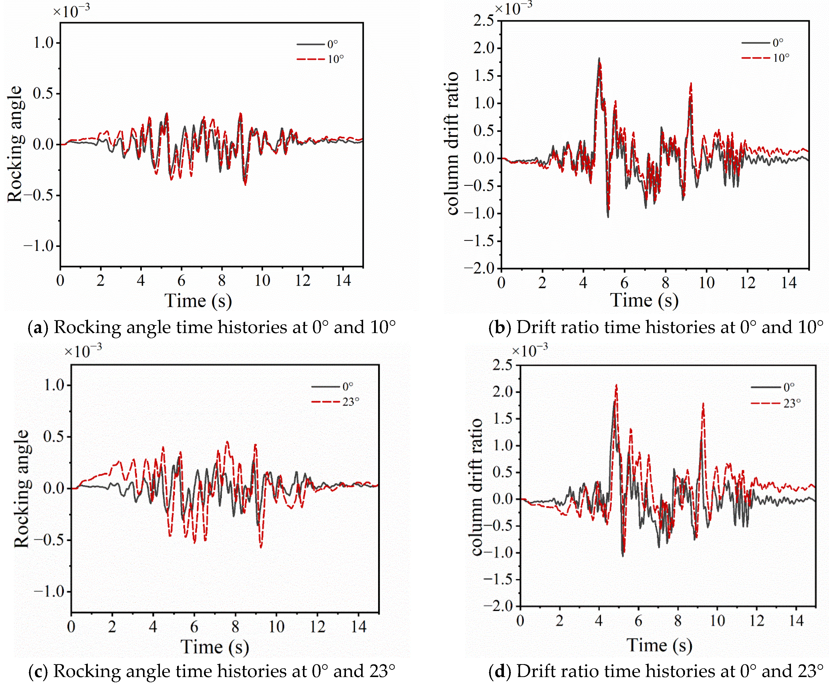
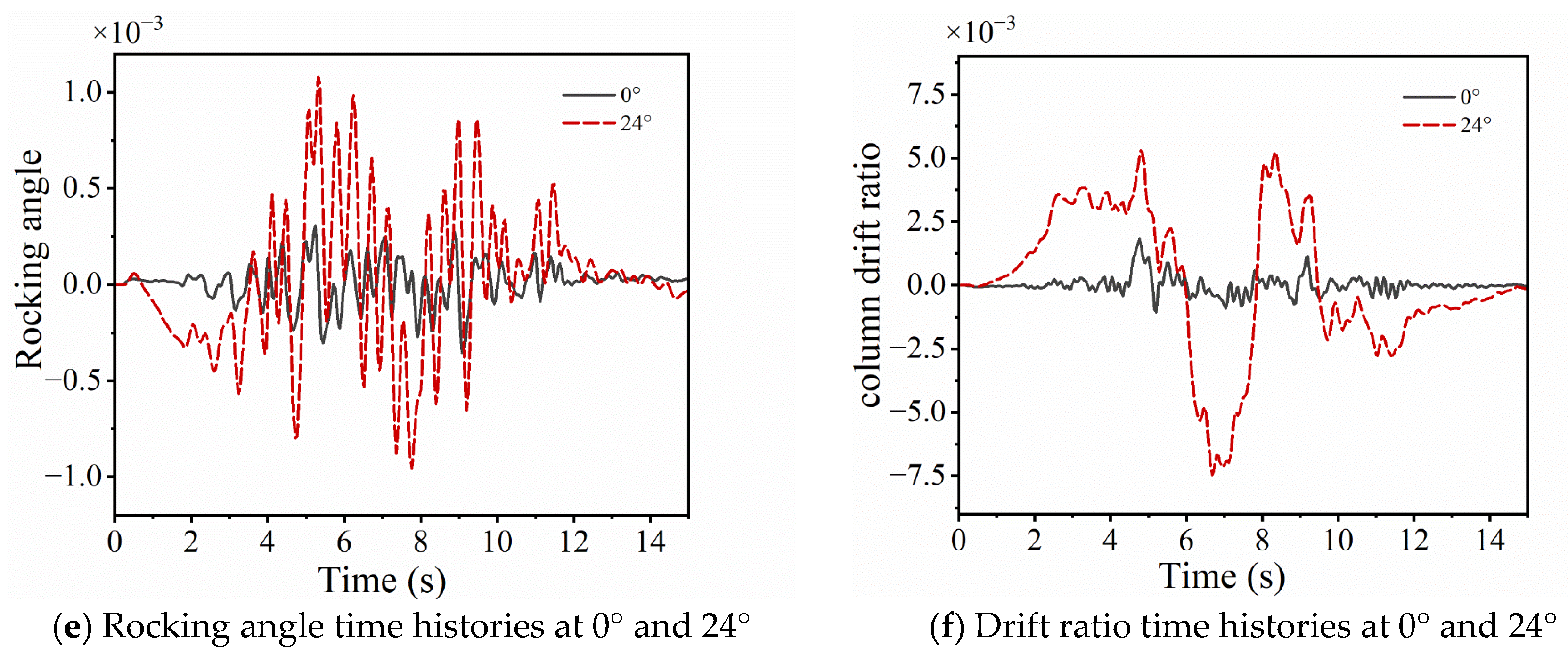
To further validate the variation observed in Figure 11, Figure 12 compares the responses of the inter-story drift ratio and rocking angle under representative incidence angles ($\alpha$ = 10°, 23°, and 24°), together with the vertical incidence case.

Figure 12. Inter-story drift ratio and rocking angle time histories under 0°, 10°, 23°, 24°.

At $\alpha$ = 10°, the time-history curves of both responses are essentially consistent with those at $\alpha$ = 0°, with a slight decrease in the amplitude of ${\theta }_{\mathrm{d}}$. When $\alpha$ increased to 23°, the time-history curves of ${\theta }_{\mathrm{r}}$ and ${\theta }_{\mathrm{d}}$ exhibited a phase difference compared with $\alpha$ = 0°. Meanwhile, the amplitude of ${\theta }_{\mathrm{r}}$ and ${\theta }_{\mathrm{d}}$ increased, indicating an enhanced contribution of the rocking response to the structural response. At $\alpha$ = 24°, ${\theta }_{\mathrm{r}}$ increases significantly, inducing additional rotation at the column ends and resulting in a marked increase ${\theta }_{\mathrm{d}}$. Overall, these time-history features indicate a progressive shift in the structural response from shear-dominated behavior toward a combined shear–rocking coupled mode.

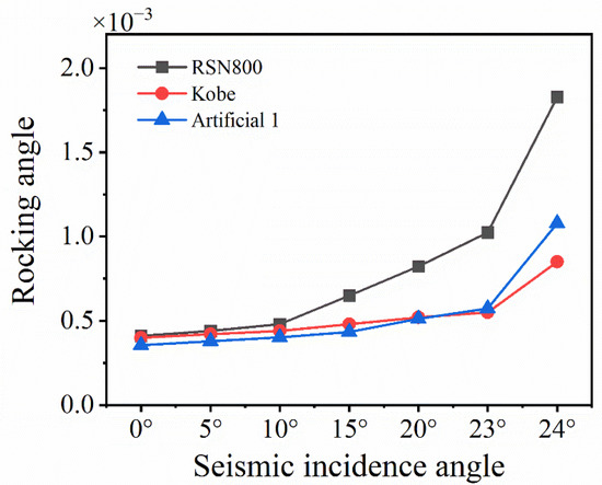
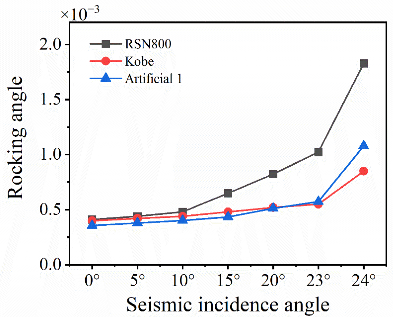
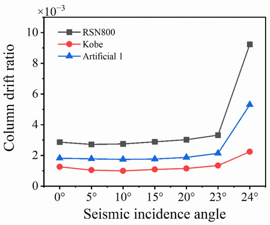
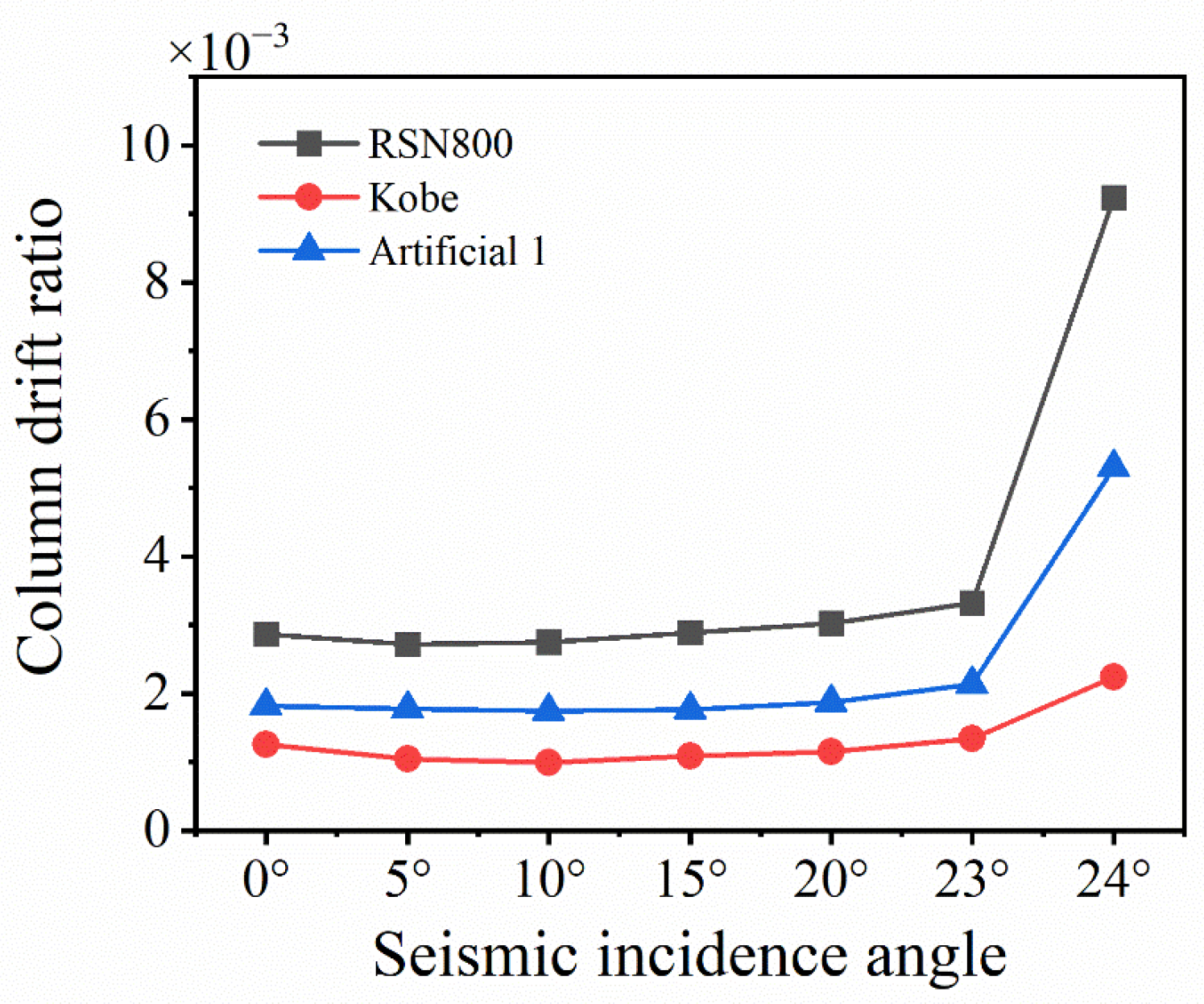
To avoid the record-specificity issue potentially introduced by a single ground motion record, two real ground motion records with spectral characteristics distinct from those of wave artificial1 were added. Under the premise of consistent site class and ground motion intensity, a parametric analysis was conducted for incident angles ranging from 0° to 24°. Figure 13 and Figure 14 show drift ratio and rocking angle versus incident angle.

Figure 13. Rocking angle versus incident angle.

Figure 14. Drift ratio versus incident angle.

The results indicate that the trends of drift ratio, rocking angle, and damage patterns obtained under different ground motions are in excellent agreement, confirming that the variation in structural response is not attributable to the ground motion characteristics, and suggesting that the amplification of structural response due to near-critical-angle oblique incidence is a general phenomenon.

3.3. Concrete Damage of Station

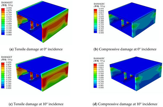
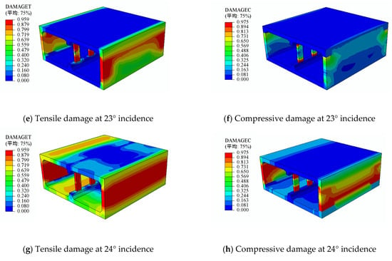
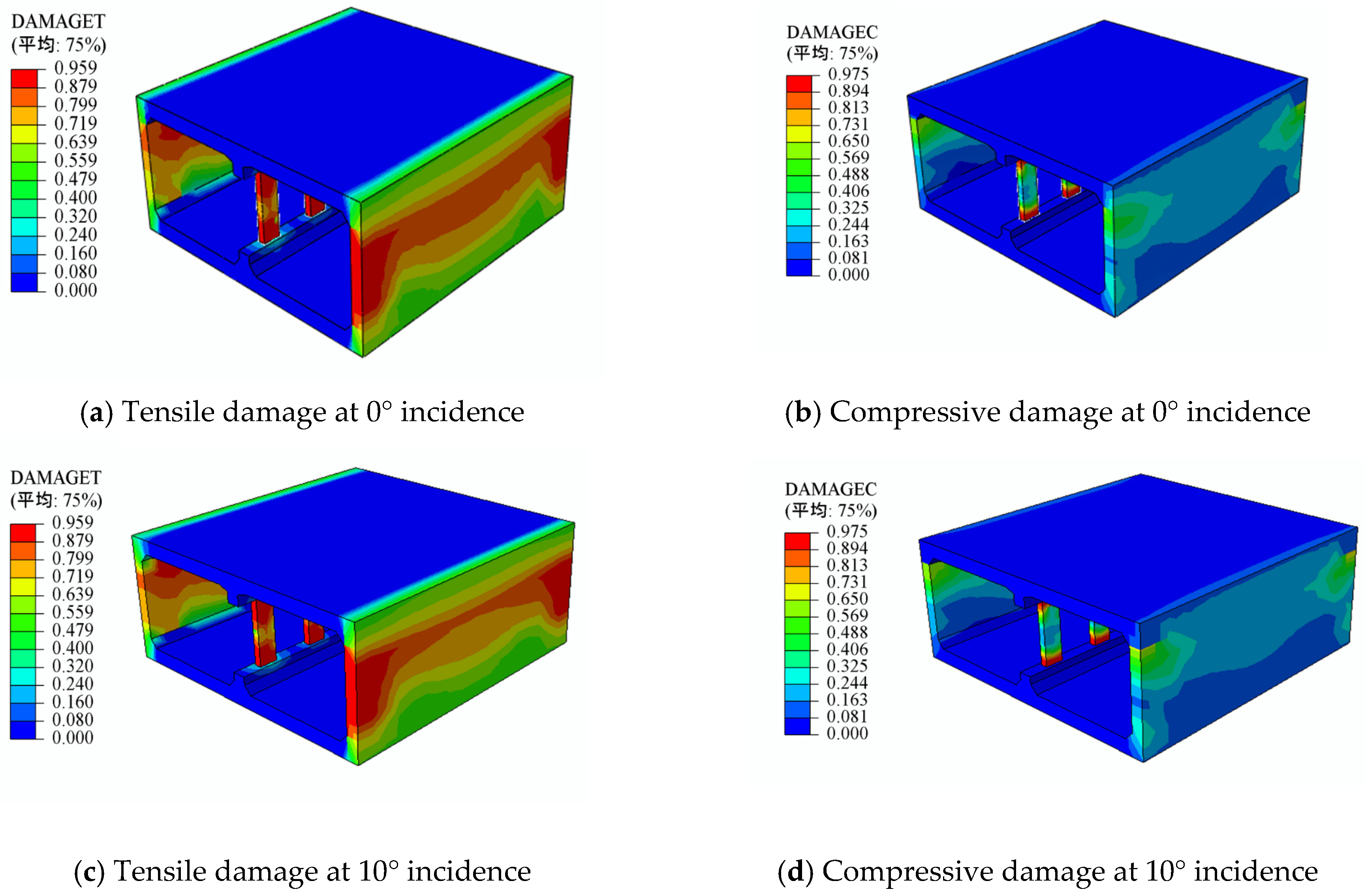
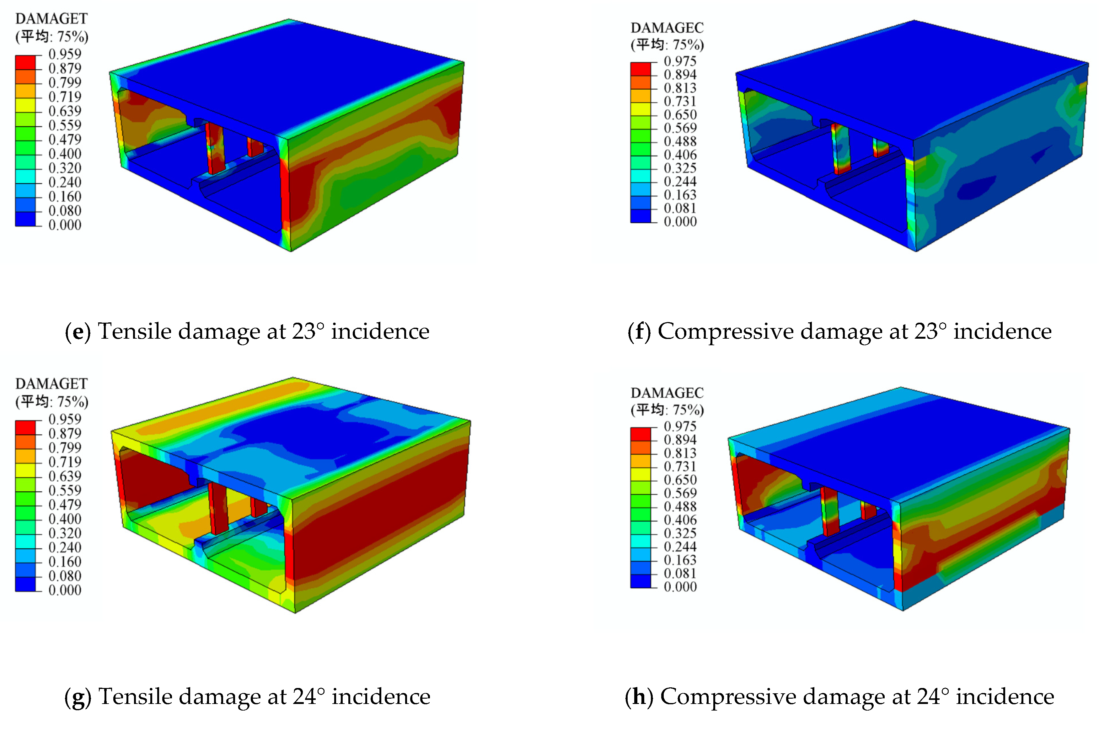
To examine the overall damage distribution of the station from 0° to 24°, Figure 15 presents the contour plot of tensile and compressive damage of the entire structure.

Figure 15. Tensile and compressive damage contours of the station from 0° to 24°.

For $\alpha$ from 0° to 23°, damage is mainly concentrated in the central columns and sidewalls. The tensile damage severity in the sidewalls reduces, and the compressive damage in columns exacerbates as $\alpha$ increases. At $\alpha$ = 24°, the overall damage changes markedly. In the central columns, tensile damage spreads from the ends toward the middle and nearly covers the entire members. Compressive damage remains concentrated at the top and bottom regions but becomes more severe. The tensile damage pattern in the sidewalls is similar to that in the columns. In contrast, compressive damage exhibits an antisymmetric distribution, concentrating at the bottom of one wall and at the top of the opposite wall. This indicates significant structural rotation. In addition, the floor slabs also exhibit severe tensile and compressive damage.

For the central columns, both tensile and compressive damage are significantly concentrated at both ends and are relatively severe, with a large proportion of severely damaged volume. For the side walls, the compressive damage is minimal, and although the tensile damage is greater than the compressive damage, the overall damage level is far lower than that of the central columns. This result is highly consistent with the field investigation of the Daikai station, where the side walls remained basically intact, and the failure was concentrated at the ends of the central columns.

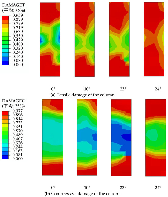
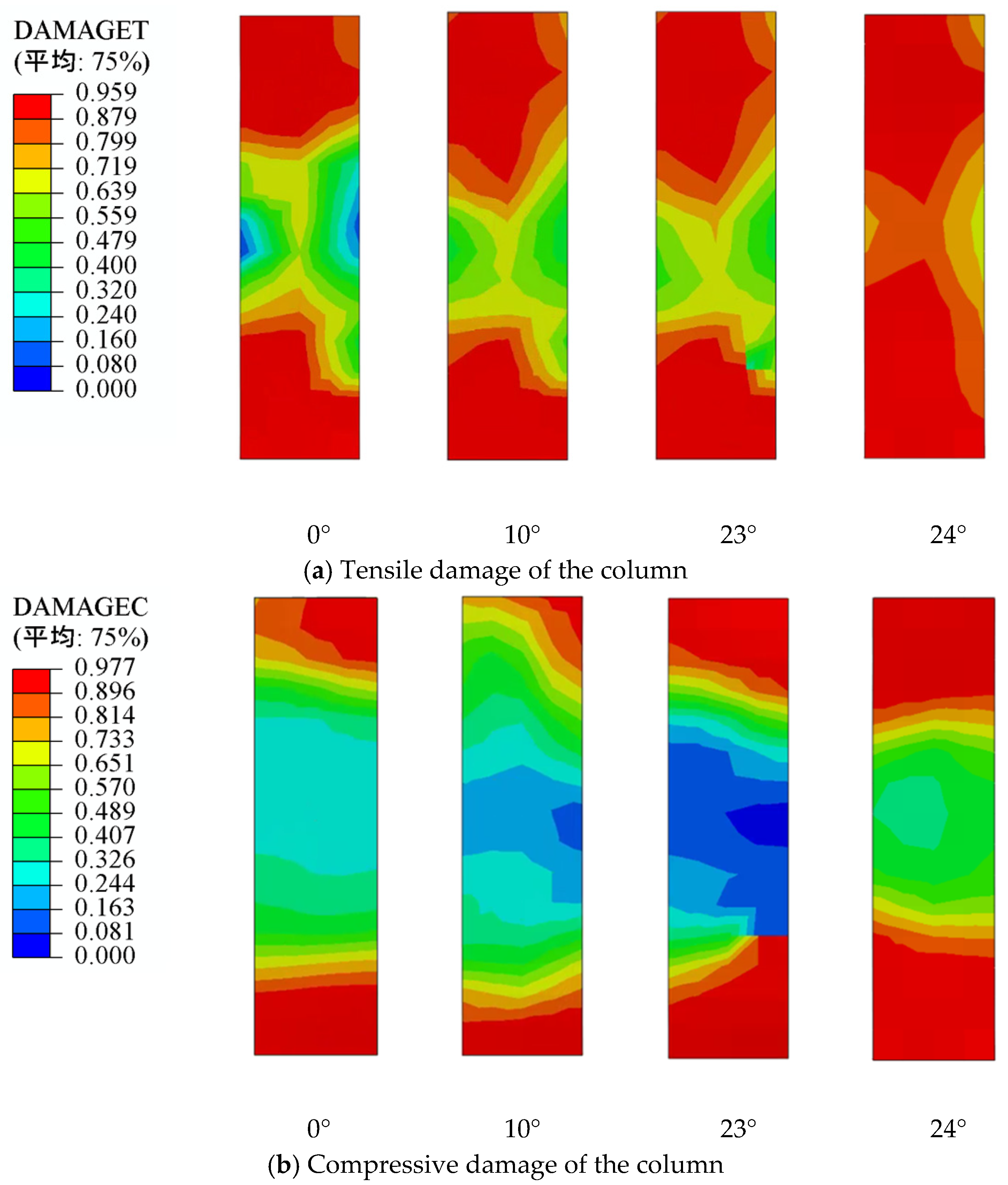
To further clarify the damage evolution of the central column, Figure 16 presents a contour plot of tensile and compressive damage in the column, reflecting the characteristics of damage patterns with increasing incidence angle. At $\alpha$ = 0° and 10°, tensile damage is mainly concentrated at the column ends, while diagonal cracking develops in the middle region. Compressive damage is also concentrated at the ends, whereas the middle region shows relatively low and uniform damage distribution. This corresponds to a typical shear-dominated response. The damage at $\alpha$ = 10° is less severe than that at $\alpha$ = 0°, consistent with the previously observed reduction in the inter-story drift ratio. This indicates a decrease in shear deformation. When $\alpha$ increases to 23°, tensile damage in the middle region further decreases. Meanwhile, compressive damage gradually accumulates and becomes more severe at the column ends. This indicates a continued reduction in shear action along with a continuous increase in rocking response. This indicates a transition from distributed shear cracking along the column body to localized compression-shear damage at the column ends. At $\alpha$ = 24°, the damage pattern changes significantly. Both tensile and compressive damage extend from the column ends toward the middle region.

Figure 16. Concrete damage contours of the central column under different incidence angles.

At $\alpha$ = 24°, the structure’s rocking response reaches its maximum. The central column experiences a massive end rotation, causing the concrete at its ends to fail due to compressive-shear crushing, which in turn leads to a sharp decline in lateral stiffness. As the inter-story drift ratio increases sharply, severe tensile and compressive damage develops along the column, ultimately resulting in a near-loss of load-bearing capacity.

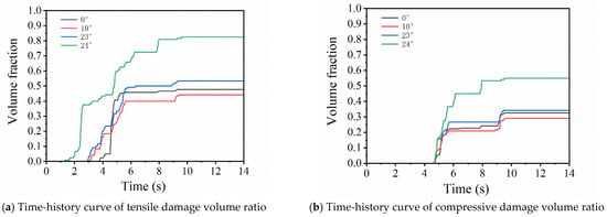
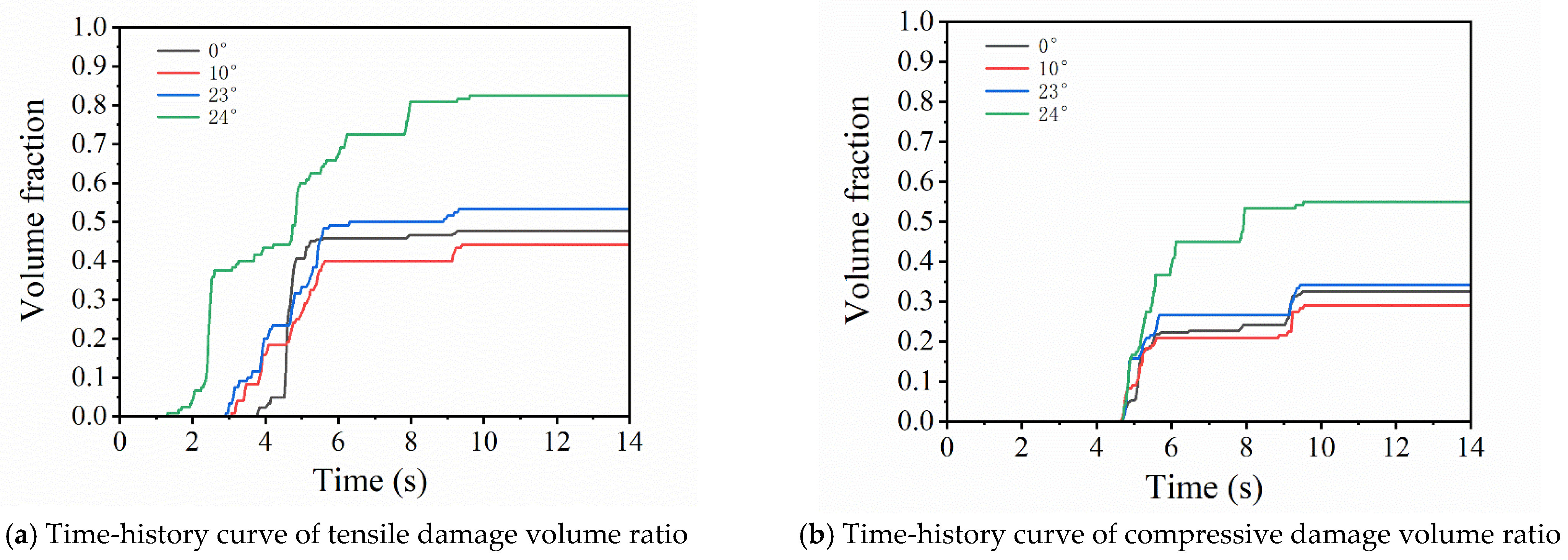
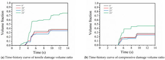
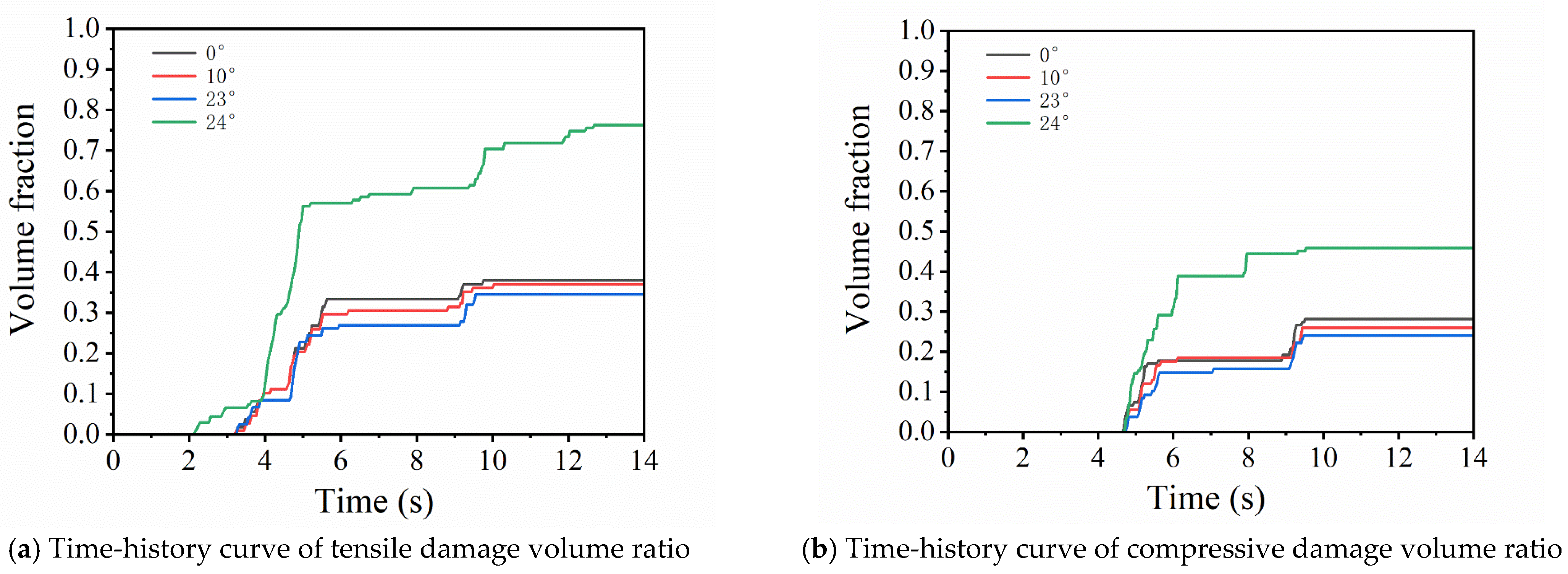
To investigate whether the progression of damage is consistent with the time histories of the swing angle and displacement angle, Figure 17 and Figure 18 further present the time-history curves of the damage volume fraction for the central column and side walls under severe damage (damage factor > 0.7), analyzing the onset and termination times of member damage and their synchronization with the structure’s peak response.

Figure 17. Damage volume ratio of the central column.

Figure 18. Damage volume ratio of the sidewall.

Comparing the damage volume ratio curves with the drift ratio and rocking angle curves reveals that tensile damage is mainly controlled by the drift ratio, while compressive damage is mainly controlled by the rocking angle. The drift ratio reaches its first major peak at 4.76 s, the second at 5.2 s, and the third at 9.24 s, which correspond one-to-one with the moments when tensile damage in the central columns increases. Meanwhile, the variation in volume ratio at different angles is consistent with the change in the peak drift ratio. The rocking angle reaches its first major amplitude at 4.72 s, the second at 5.2 s, and the third at 9 s; additionally, at 24°, a relatively large amplitude also appears at 7.76 s, and its amplitude variation is consistent with the change in compressive damage in the central columns. Compared with those of the central columns, the damage volume ratios of the side walls exhibit a certain reduction in amplitude, and both the tensile and compressive damage decrease continuously from 0° to 23°.

4. Assessment of Seismic Resilience of Subway Stations

4.1. Vulnerability Analysis of the Station

For assessing the structure’s seismic resilience, analyses are conducted for all 11 records at two representative incidence angles. The vertical incidence case is used as the baseline condition, which is commonly adopted in conventional seismic resilience assessments. In addition, the near-critical incidence angle α = 24°, identified in this study as the most unfavorable case, is selected as the key scenario for comparison.

In frame-type subway stations, the central column constitutes the dominant vertical load-bearing element. Its damage state directly governs the global seismic behavior of the station. The sidewalls are also the main lateral-force-resisting component. Their damage evolution has a significant influence on stiffness degradation and post-earthquake recoverability. Accordingly, the inter-story drift ratios of the central columns and sidewalls are adopted as EDPs for quantitative damage assessment.

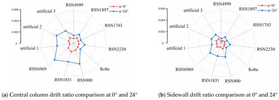
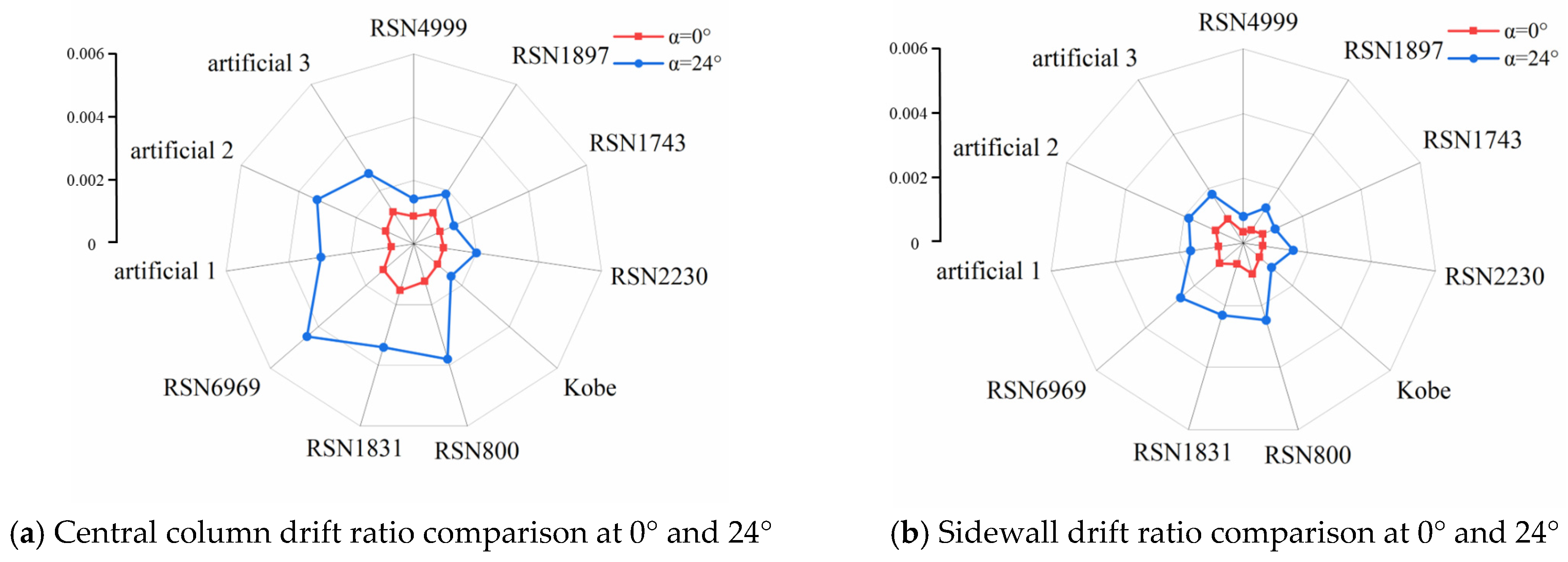
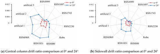
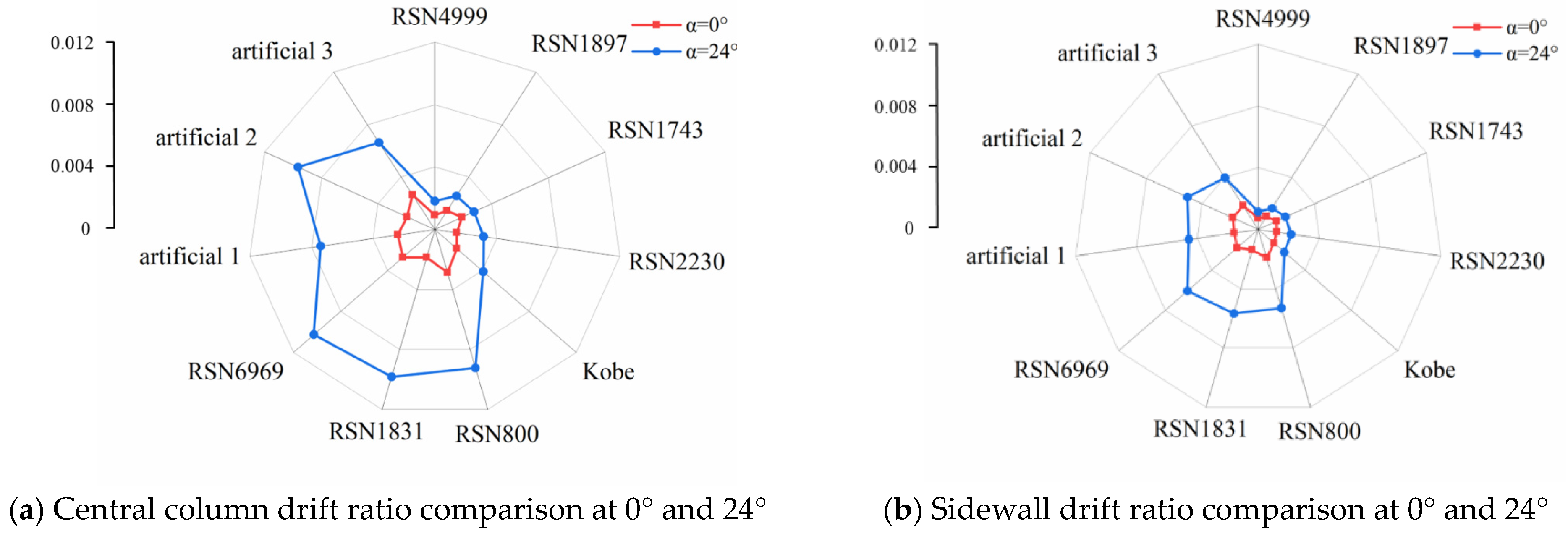
Figure 19 shows the drift ratio comparison of the central column and side wall under 11 ground motions at α = 24° and α = 0° for the design basis earthquake (PGA = 0.2 g), while Figure 20 shows the corresponding results for the rare earthquake (PGA = 0.4 g). Overall, the drift ratios of both the central column and sidewalls increase when $\alpha$ from 0° to 24°. across all ground motions. This indicates that, under the conditions considered in this study, near-critical-angle oblique incidence generally amplifies the structural response, leading to increased deformation in key vertical members.

Figure 19. EDPs under design basis earthquakes.

Figure 20. EDPs under rare earthquakes.

To quantitatively assess the damage state of subway stations under different seismic actions, it is necessary to establish clear damage classification criteria based on EDP. This section references the research findings of Du [45] and categorizes the seismic performance of the station into five levels: essentially intact, minor damage, moderate damage, severe damage, and collapse. The drift ratio thresholds corresponding to each state are presented in Table 4.

Table 4. Drift ratio ranges for different damage grades.

Damage State	Damage Condition	Drift Ratio Range
State 0	Essentially intact	θ ≤ 0.0005
State 1	Minor damage	0.0005 < θ ≤ 0.0021
State 2	Moderate damage	0.0021 < θ ≤ 0.0046
State 3	Severe damage	0.0046 < θ ≤ 0.0072
State 4	Collapse	0.0072 < θ

Where θ denotes the drift ratio.

This study’s assessment of seismic resilience follows the methodology provided in the GB/T 38591–2020. In accordance with Appendix G of this standard, a probabilistic analysis framework based on Monte Carlo simulation is adopted for the resilience assessment.

First, an expansion of EDPs is carried out. The n time-history analyses yield m EDPs, which are assembled into a matrix $X$ of size $n\times m$. Under a specified seismic wave intensity, the distribution of EDPs can usually be approximated by a lognormal distribution. Taking the natural logarithm of every element in $X$ produces the log-transformed data matrix $Y$, and the covariance matrix ${\mathsf{\Sigma }}_{YY}$ of $Y$ is then computed. To generate simulated samples that preserve the same correlation structure in subsequent steps, the positive-definite covariance matrix ${\mathsf{\Sigma }}_{YY}$ is decomposed using Cholesky factorization:

$$Y=\mathrm{l}\mathrm{n}X$$

(23)

$${\mathsf{\Sigma }}_{YY}=L{L}^T$$

(24)

where $Y$ is the log-transformed data matrix. According to the central limit theorem and the properties of the lognormal distribution, $Y$ follows a multivariate joint normal distribution. $L$ is the lower triangular matrix, which serves as a linear transformation matrix to impose the same covariance structure as the original data onto the random samples.

By introducing an independent standard normal vector $\mathrm{U}=[U_1,U_2,\dots ,U_m{]}^{\mathrm{T}}$, expanded samples in the logarithmic space are generated. The expanded EDP sample vector $Z$ in the logarithmic space is obtained as:

$$Z=LU+M_Y$$

(25)

where $M_Y$ is the mean vector of matrix $Y$; $Z$ is a random vector following a multivariate normal distribution with mean $M_Y$ and covariance ${\mathsf{\Sigma }}_{YY}$.

Exponentiating each element of $Z$ yields a set of EDP values in the original physical dimensions with the correct correlation structure. Repeating this random sampling procedure $N_{\mathrm{sim}}$ times produces the complete simulated matrix:

$$X^{\mathrm{sim}}=\exp \left(Z\right)$$

(26)

where $N_{\mathrm{sim}}$ is the number of Monte Carlo simulations.

Subsequently, a component fragility model is established. Following the recommendations in Appendix G.3 of GB/T 38591–2020, an analytical fragility function based on the lognormal distribution assumption is adopted. For a given demand level $W$, the probability $P_i$_i that the interior column reaches or exceeds damage state ds_i is expressed as:

$$P_i(DS\ge d{s}_i\mid W)=\mathsf{\Phi }\left({\displaystyle \frac{\mathrm{l}\mathrm{n}(W/{\theta }_i)}{{\beta }_i}}\right)$$

(27)

where $DS$ is the damage state variable of the component; $d{s}_i$ is the specific limit value defined for the i-th damage state; $\mathrm{W}$ is the engineering demand parameter of the structure; ${\mathsf{\theta }}_{\mathrm{i}}$ is the damage threshold for the i-th damage state; ${\beta }_i$ is the logarithmic standard deviation for the i-th damage state; and $\mathsf{\Phi }$ is the cumulative distribution function of the standard normal distribution.

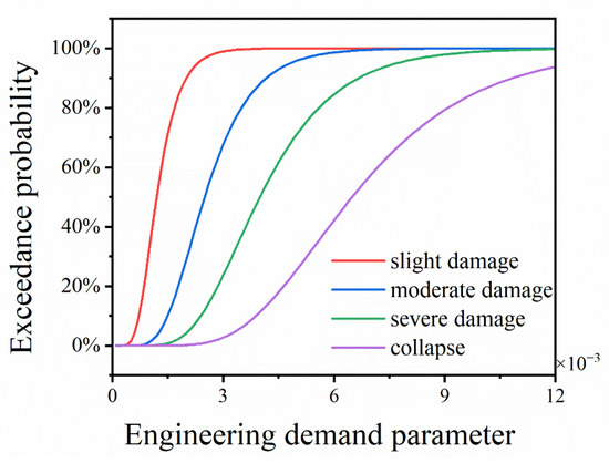
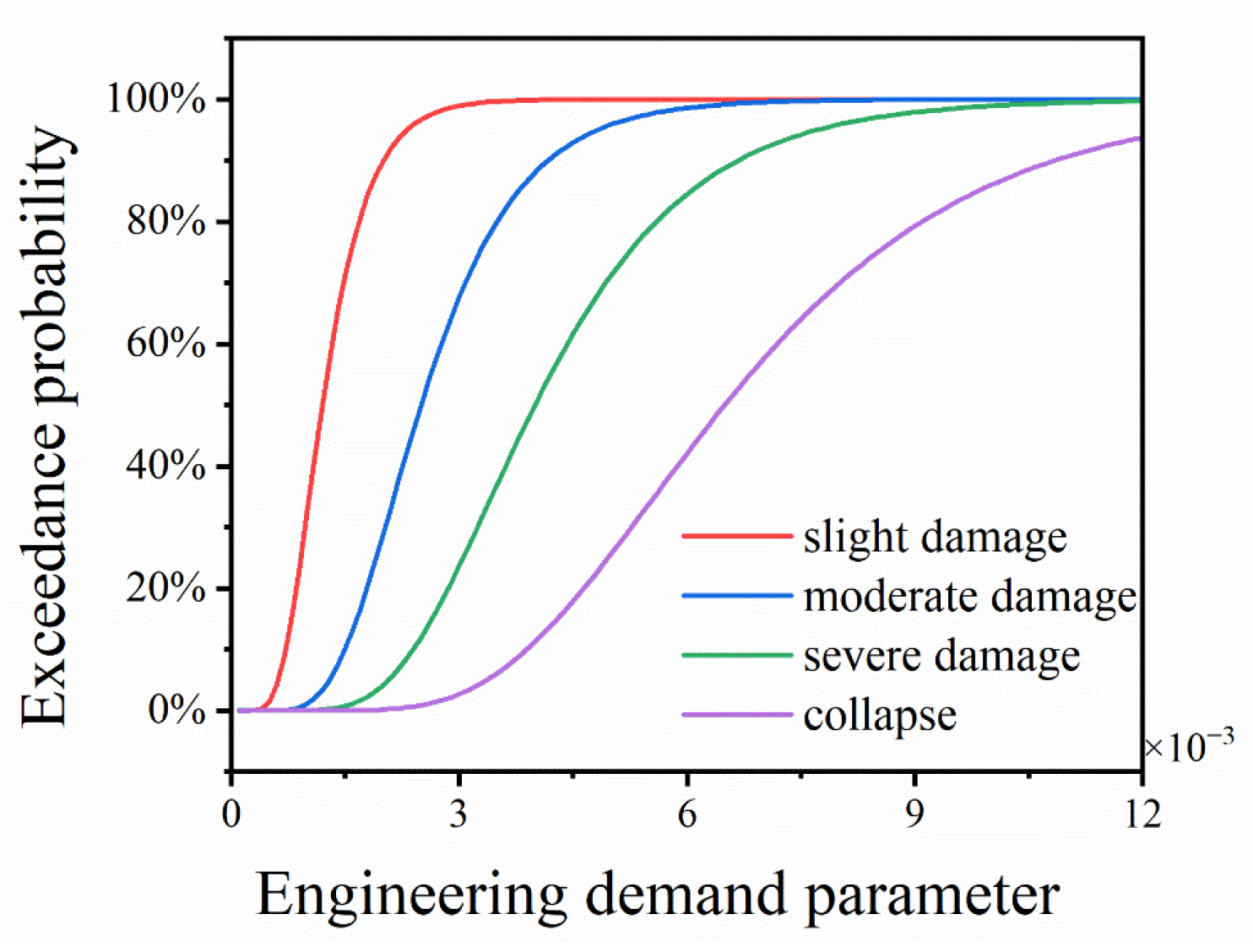
The damage-state exceedance probability conditional on EDP obtained from 2000 Monte Carlo simulations based on Equation (27) is shown in Figure 21.

Figure 21. Damage state exceedance probability conditional on EDP.

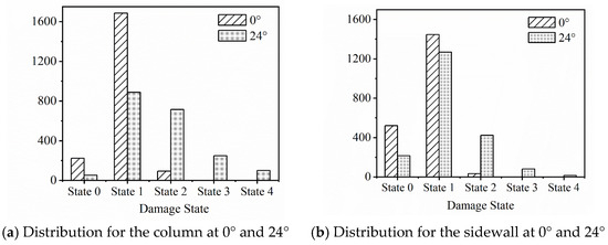
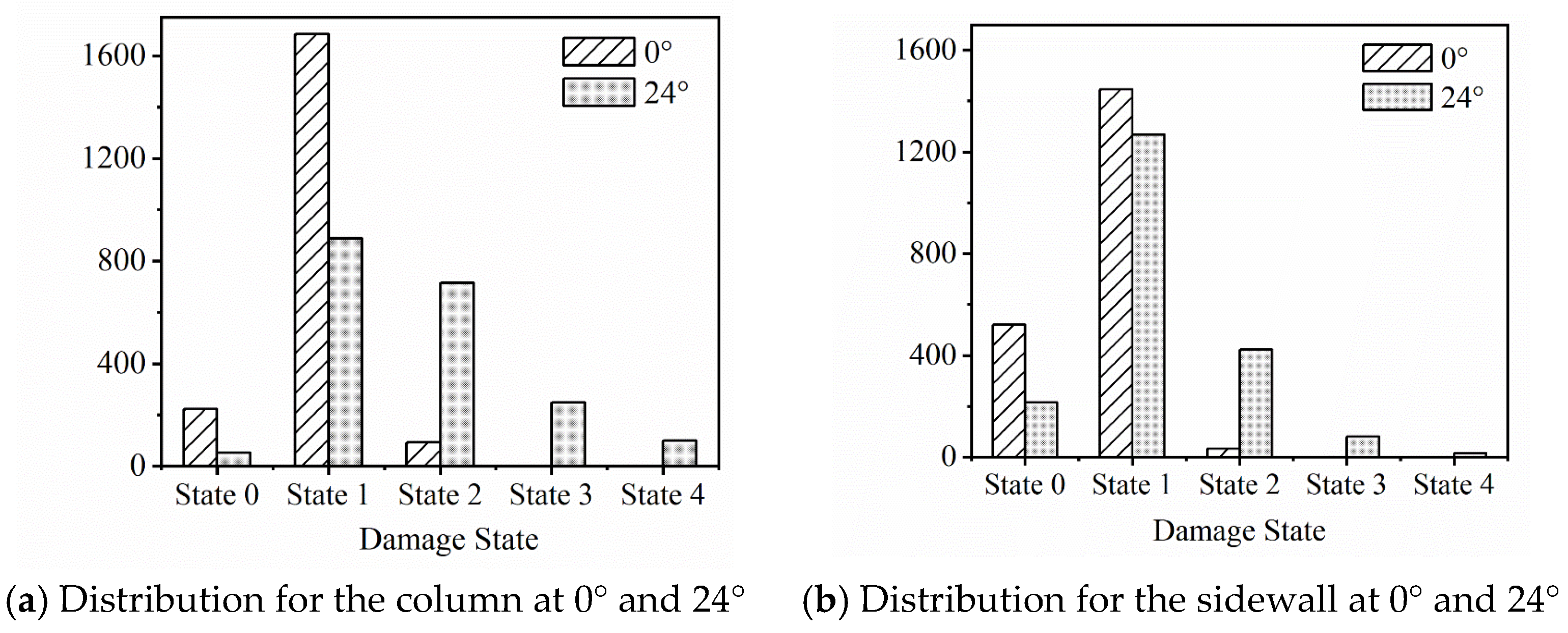
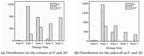
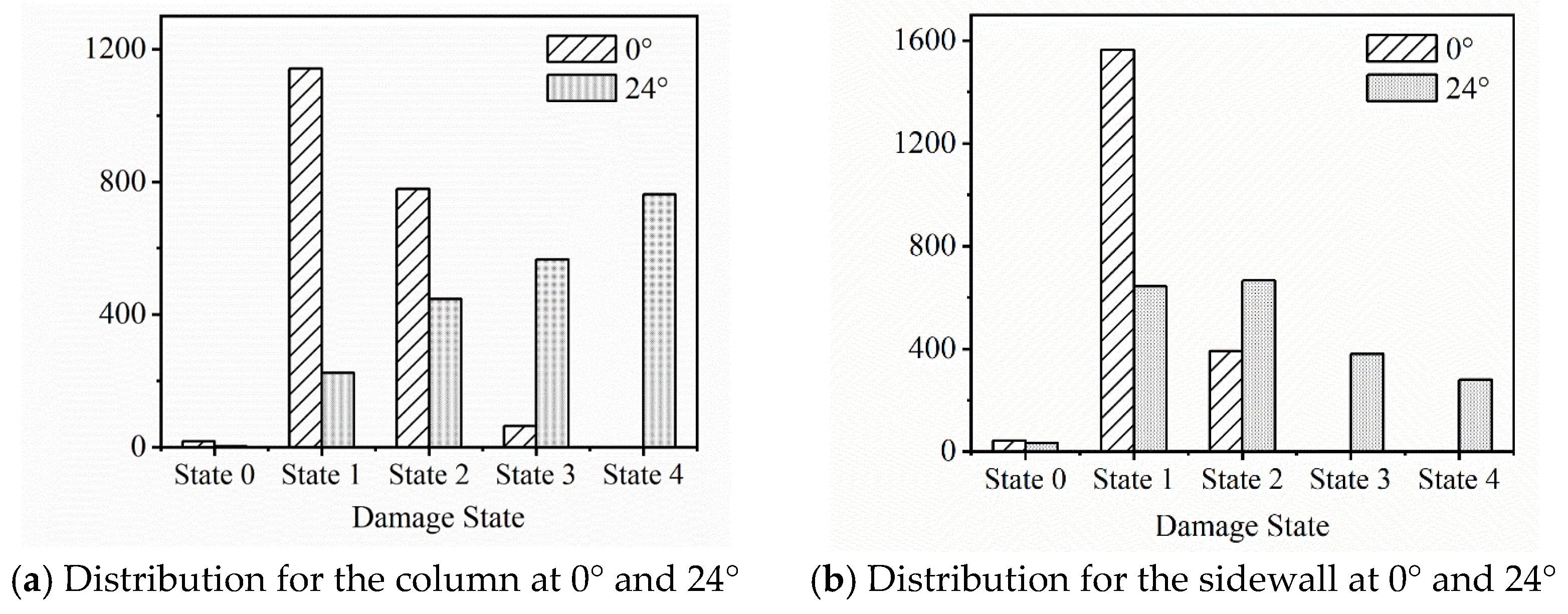
Figure 22 and Figure 23 present the damage state distributions of the structure under design basis earthquakes and rare earthquakes, respectively. Under the design basis earthquakes, the damage of both the central column and sidewall is dominated by State 1 at α = 0, indicating an overall low damage state. As α increases to 24°, the damage severity of both the central column and sidewall increases markedly, with higher damage states observed. Under the rare earthquake, at α = 0°, the central column and sidewalls primarily exhibit State 1 and State 2 damage. When α increases to 24°, both the central column and sidewalls sustain severe damage; the proportion of higher-state damage in the central column reaches 66.4%, and that in the sidewalls reaches 33%. The structural damage state is dominated by severe damage.

Figure 22. Damage grade distribution under the design basis earthquakes.

Figure 23. Damage grade distribution under the rare earthquakes.

On the basis of the acquired damage state, the resilience of the station is quantified using three indicators: repair costs, repair time, and casualties—in accordance with GB/T 38591–2020. Appendix A.5.4 of the standard specifies that a lognormal distribution model shall be adopted to fit the set of seismic resilience indicators, and that the fitted values corresponding to the 84th percentile shall be used as the basis for seismic resilience assessment.

4.2. Economic Losses

Economic loss is evaluated using the ratio of repair costs to total structural cost, denoted as κ. The repair cost index for each simulation is calculated as follows:

$$\kappa ={\displaystyle \frac{{\lambda }_i·{\sum }_{j=0}^m{C}_{(i,j)}·{\eta }_{1(i,j)}·{\eta }_{2(i,j)}}{C_{\mathrm{T}}}}$$

(28)

where $C_{\left(i,j\right)}$ represents the repair cost of component $j$ at damage state $i$, calculated according to current standard unit rates, with HRB400 steel reinforcement priced at 3600 CNY/t and C40 concrete at 500 CNY/m³; ${\eta }_{1(i,j)}$ is the damage coefficient for component $j$ in damage state $i$, taken from GB/T 38591–2020; ${\eta }_{2(i,j)}$ is the repair coefficient for component $j$ under damage state $i$, also taken from GB/T 38591–2020; ${\lambda }_i$ is the economic loss repair coefficient introduced to account for the complexity of underground structure repair work, with values taken from Yang et al. [14]: 1.0 for damage states below 2 and 2.0 for damage at state 2 or above; $C_T$ represents the total construction cost of the building structure, calculated according to current standard rates.

Since the distribution of the resilience index contains a proportion of zero values, and the log-normal distribution is defined only on the positive real line, it cannot represent exact zeros. Consequently, forcing a log-normal fit would distort the cumulative probability mass near zero. Based on this, a zero-inflated log-normal distribution is adopted. In this formulation, the probability at zero is directly estimated from the empirical proportion of zero values, while the non-zero portion is determined by the log-normal distribution of the sample. This framework explicitly preserves the probability at zero and reduces the systematic bias that may result from incorrect distribution assumptions.

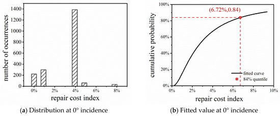
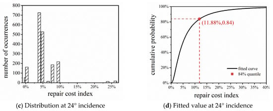
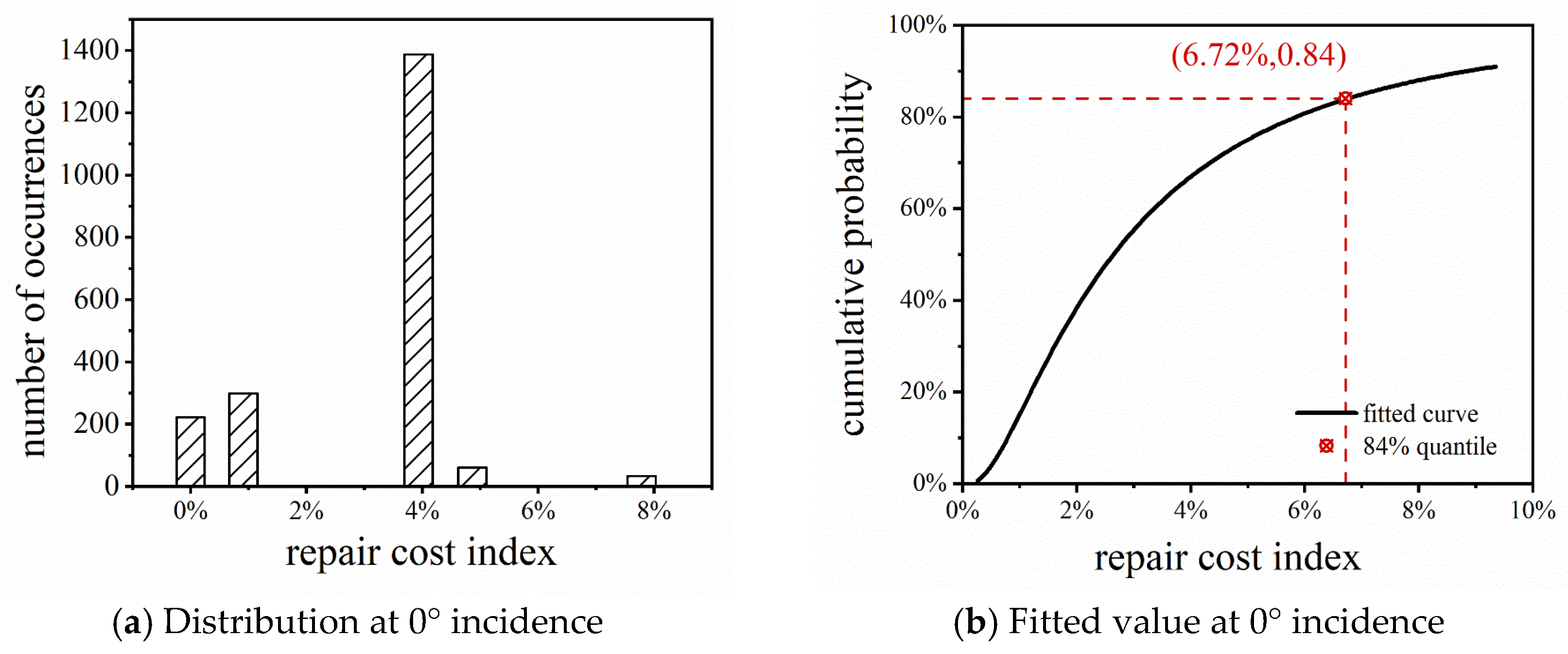
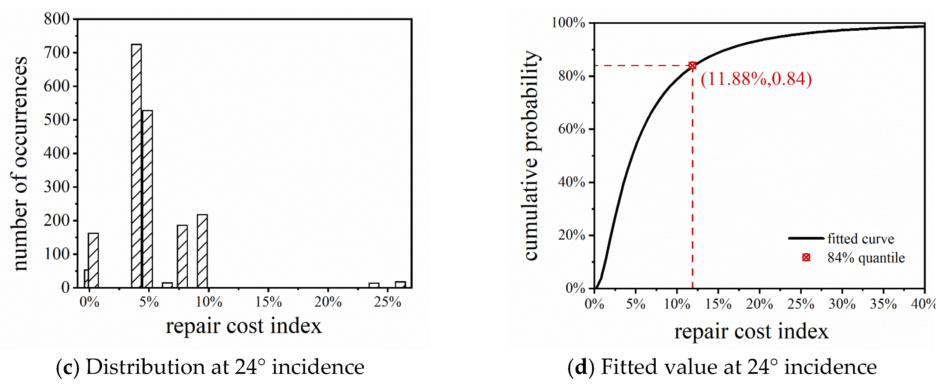
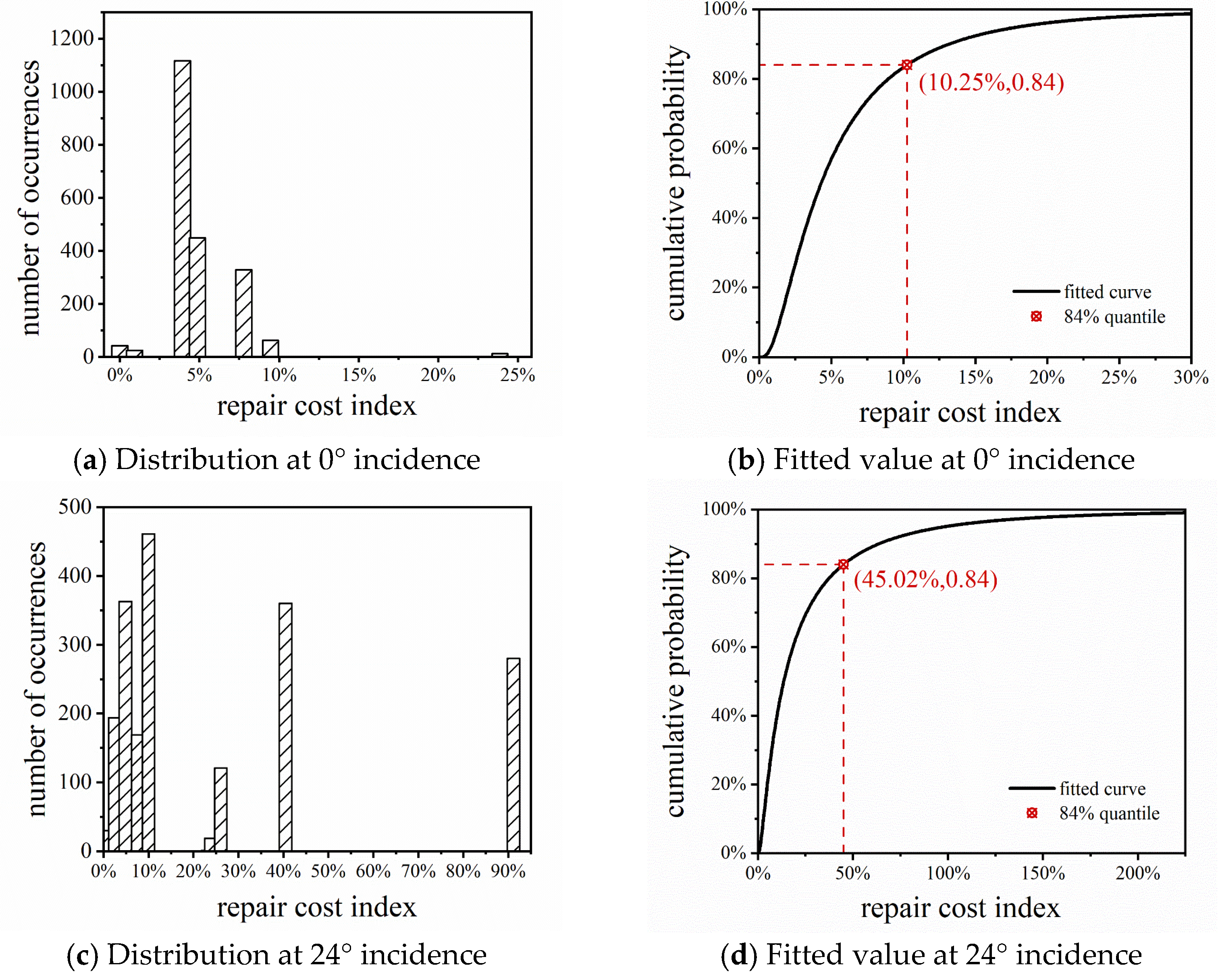
Based on the repair cost index values obtained from 2000 Monte Carlo simulations, a zero-inflated log-normal was used to fit the data, and the 84th percentile was extracted as the benchmark for resilience assessment. The distributions of the repair cost index and the fitted curves under design basis earthquakes and the rare earthquakes are shown in Figure 24 and Figure 25.

Figure 24. Repair costs under design basis earthquakes.

Figure 25. Repair costs under rare earthquakes.

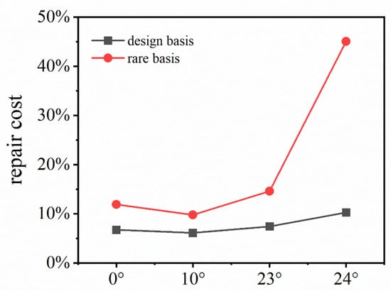
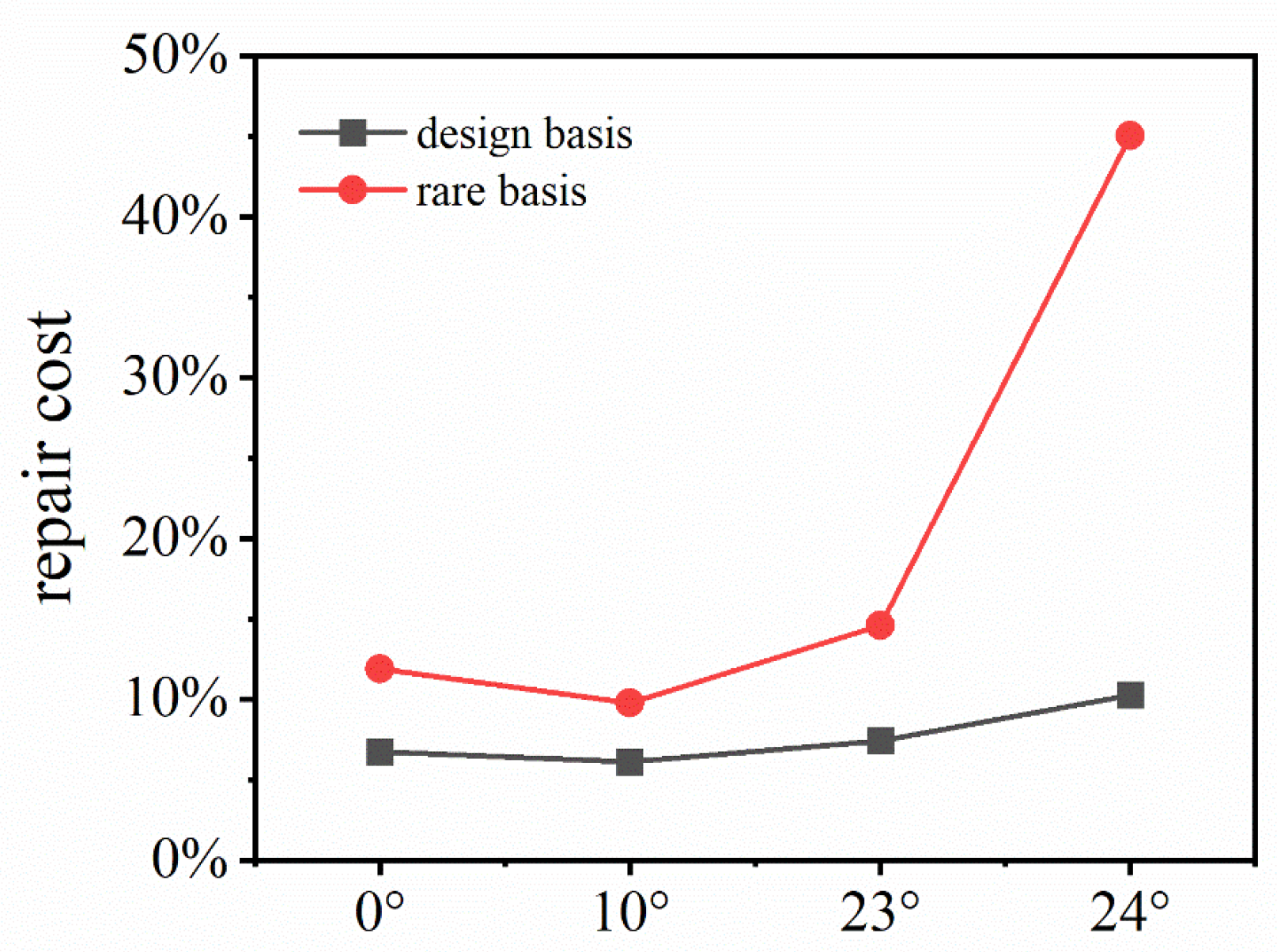
Under the design basis earthquake, the repair cost index of the station structure is 6.72% at $\alpha$ = 0° and 11.88% at $\alpha$ = 24°, representing an increase of 76%. Under the rare earthquake, the repair cost index is 10.25% at $\alpha$ = 0° and 45.02% at $\alpha$ = 24°, representing an increase of 339%.

4.3. Repair Time

The repair time index $T$ is measured in days and represents the construction period required to restore normal functionality after an earthquake. The basic formula for the repair time of the $k$-th layer is:

$$T_k={\displaystyle \frac{{\lambda }_t·{\sum }_{j=1}^n\left.\left[ Q_{(i,j,k)}·n_{(i,j,k)}\right.\right]·{\zeta }_{T\left(i\right)}·{\lambda }_{T\left(k\right)}}{N_k}}$$

(29)

$$N_k=0.026A_{k }$$

(30)

where $Q_{(i,j,k)}$ represents the repair time required for the j-th type of component at the k-th story under damage state i, expressed in man-days, with values determined according to the code [38]; $n_{\left(i,j,k\right)}$ represents the number of components of class $j$ under the same damage state $i$ and floor $k$; ${\zeta }_{T\left(i\right)}$ is the repair man-hour reduction factor, used to account for the impact of the repair workload of seismic-damaged members of class $j$; for the subject of this study, ${\zeta }_{T\left(i\right)}=1$ is adopted in accordance with the code; ${\lambda }_{T\left(k\right)}$ is the influence coefficient of floor location $k$ on seismic-damaged members, with ${\lambda }_{T\left(i\right)}$ taken as 1 according to the code; $N_k$ is the maximum number of workers accommodated per floor; ${\lambda }_t$ is the repair time correction factor introduced to account for the complexity of underground structure repairs, taken as ${\lambda }_t=1.7$ based on Yang et al. [14]; $A_k$ is the floor area of the $k$-th floor.

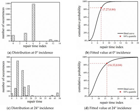
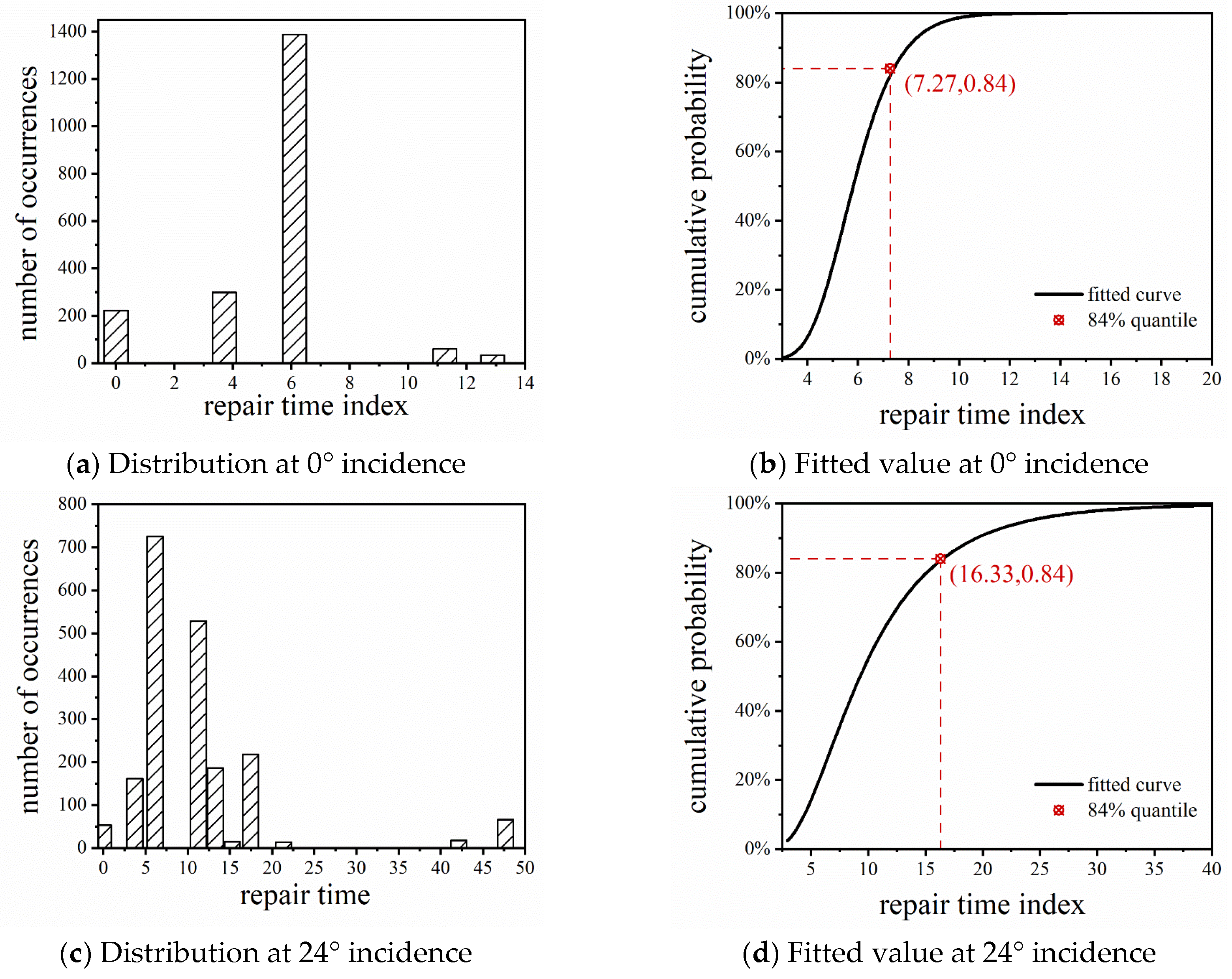
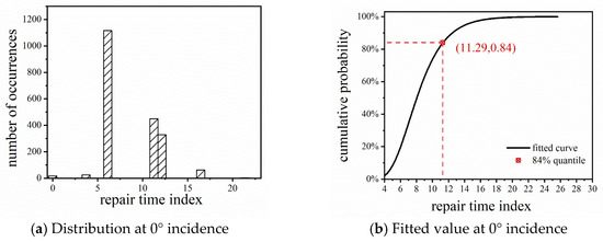
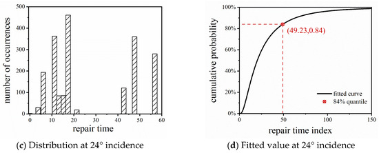
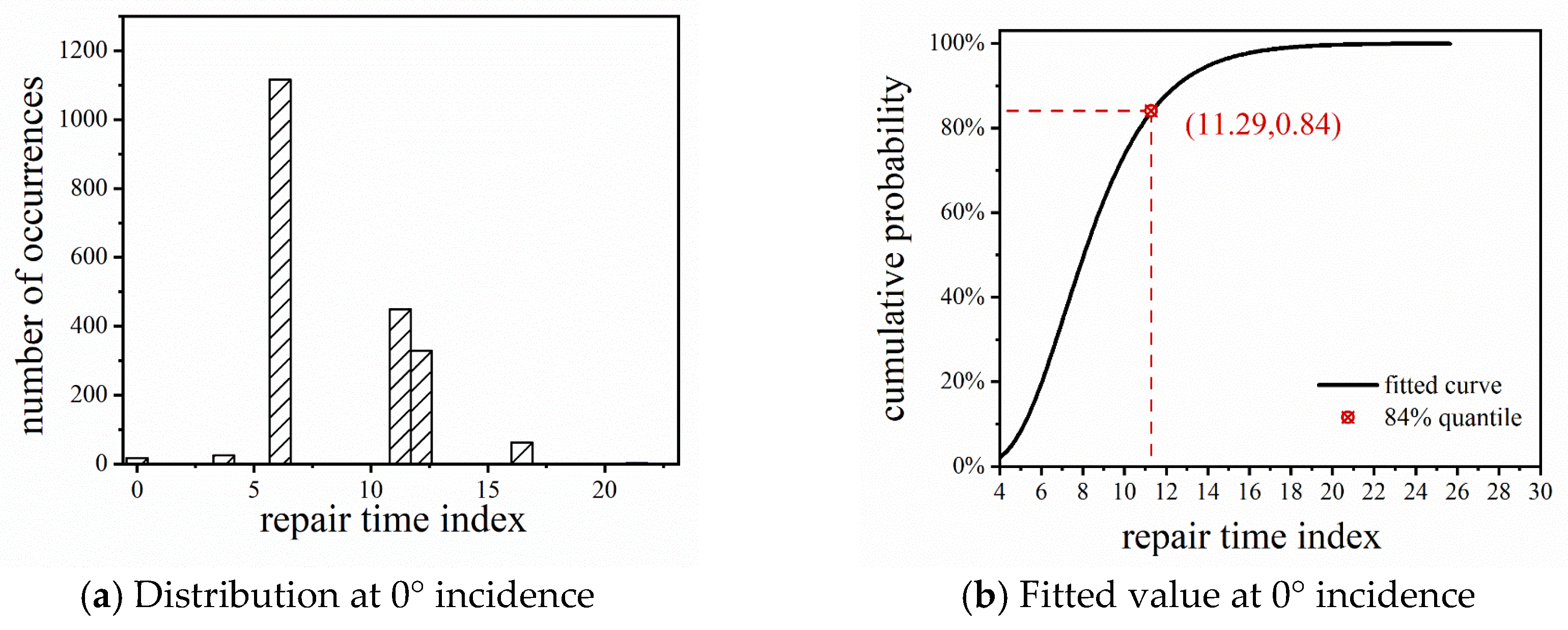
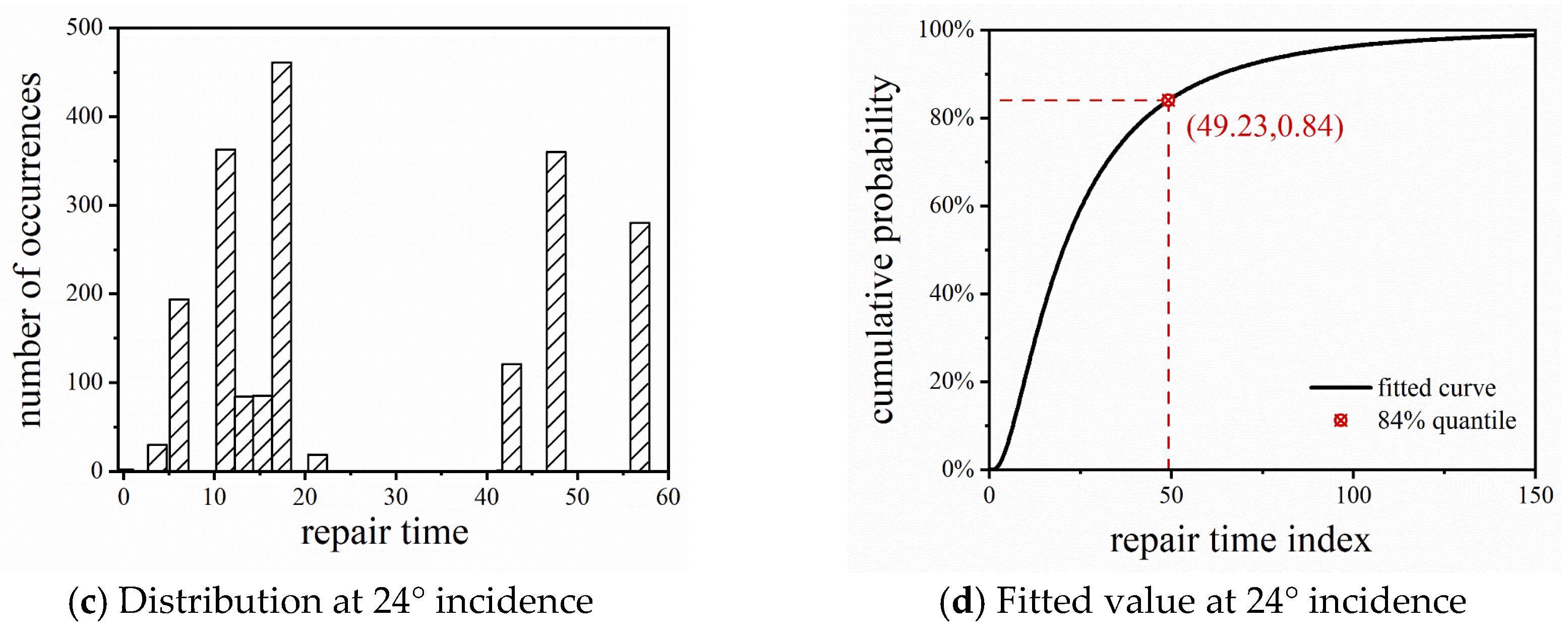
The distribution of the repair time index and the fitted curves under design basis earthquakes and the rare earthquakes are shown in Figure 26 and Figure 27.

Figure 26. Repair time under design basis earthquakes.

Figure 27. Repair time under rare earthquakes.

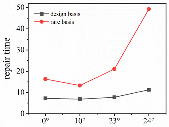
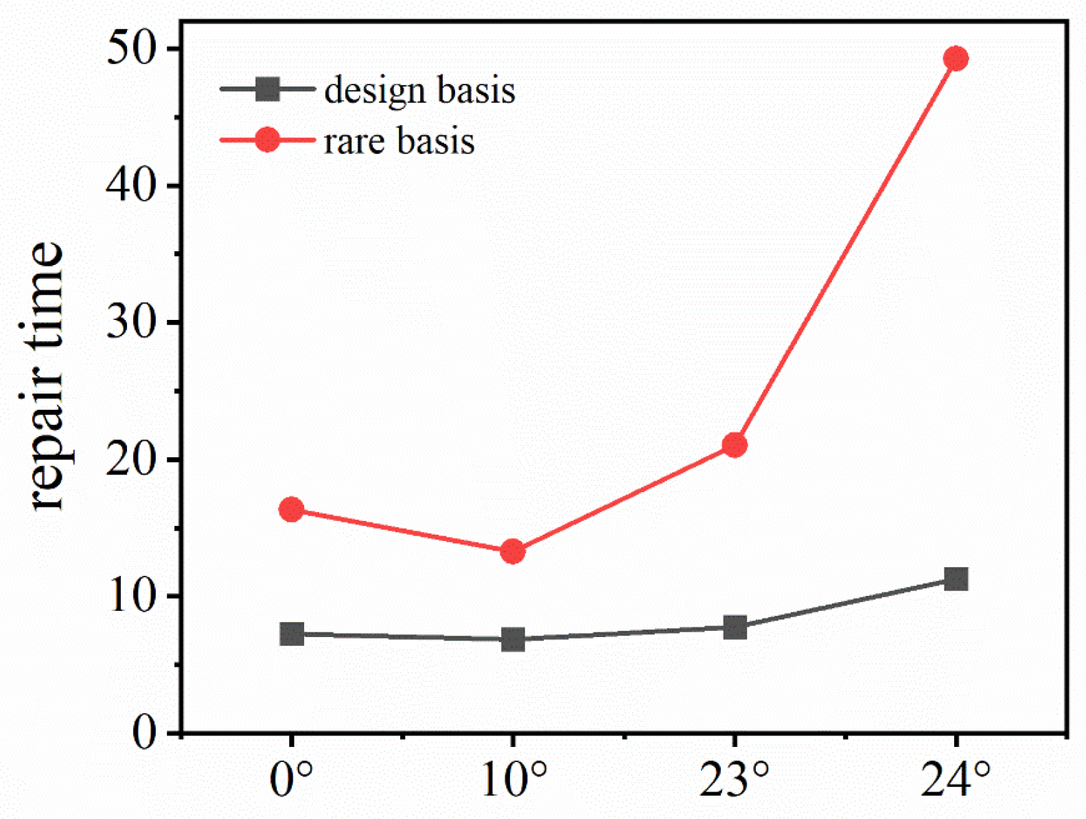
Under the design basis earthquake, the repair time index of the station structure is 7.27 d at $\alpha$ = 0° and 16.33 d at $\alpha$ = 24°, representing an increase of 124%. Under the rare earthquake, the repair time index is 11.29 d at $\alpha$ = 0° and 49.23 d at $\alpha$ = 24°, representing an increase of 336%.

4.4. Injury and Fatality

The injury rate ${\gamma }_h$ and fatality rate ${\gamma }_d$ are defined as the ratios of the number of people injured and killed during an earthquake to the total number of people in the building. These metrics reflect the level of resilience from a human safety perspective. The calculation formulas are as follows:

$${\gamma }_h={\displaystyle \frac{{\sum }_1^k{\eta }_{h(i,k)}{·\zeta }_k·A_{k }}{N_s}}$$

(31)

$${\gamma }_d={\displaystyle \frac{{\sum }_1^k{\eta }_{d(i,k)}{·\zeta }_k·A_{k }}{N_s}}$$

(32)

where ${\eta }_{h(i,k)}$ and ${\eta }_{d(i,k)}$ are the nominal injury rate and nominal fatality rate for floor $k$ under damage state $i$, taken from the code [43]; ${\zeta }_k$ is the floor occupancy density; since the subject of this study is a subway platform, it is taken as 0.5 persons/m²; and $N_s$ is the total number of people.

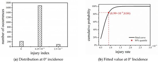
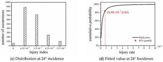
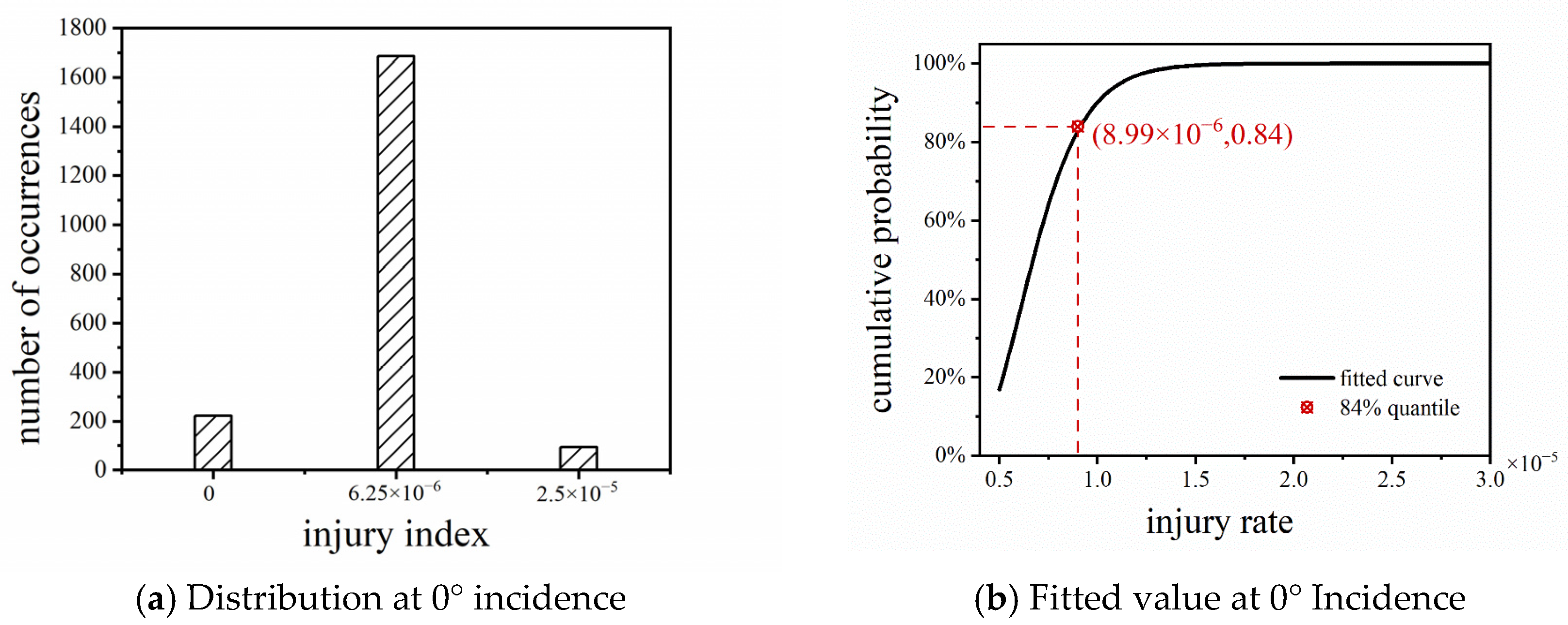
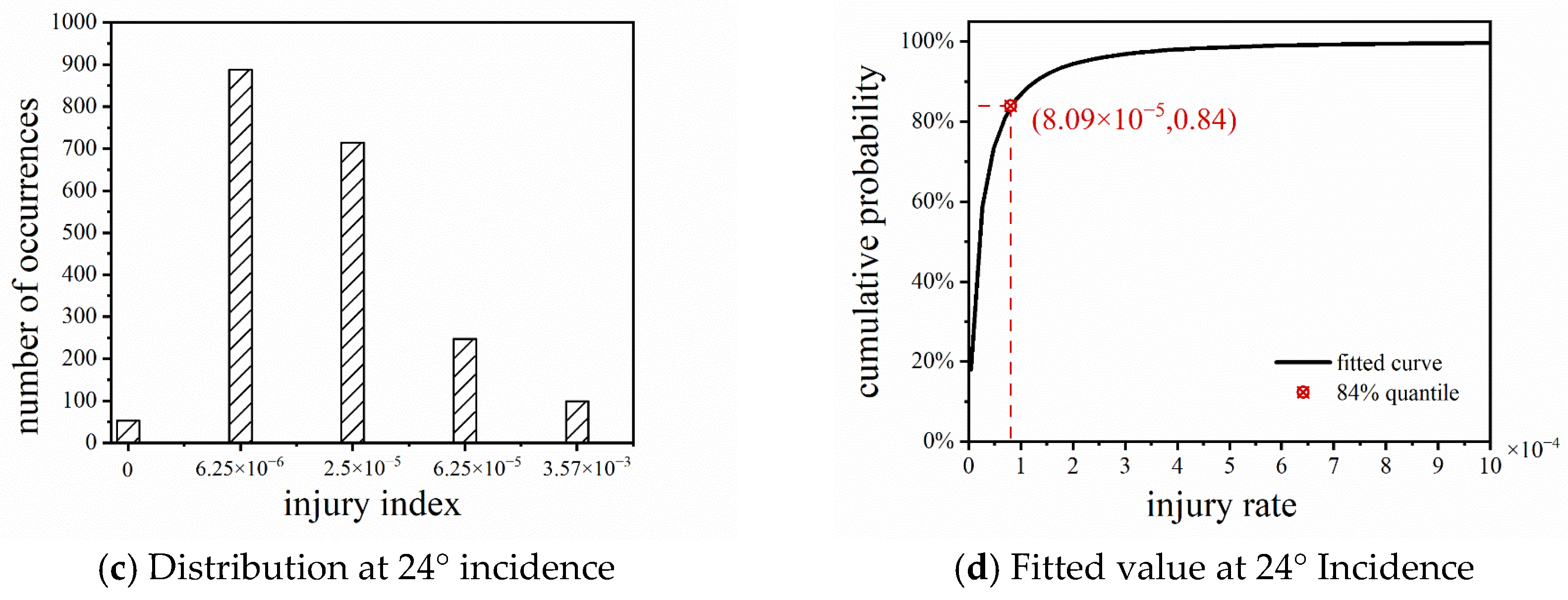
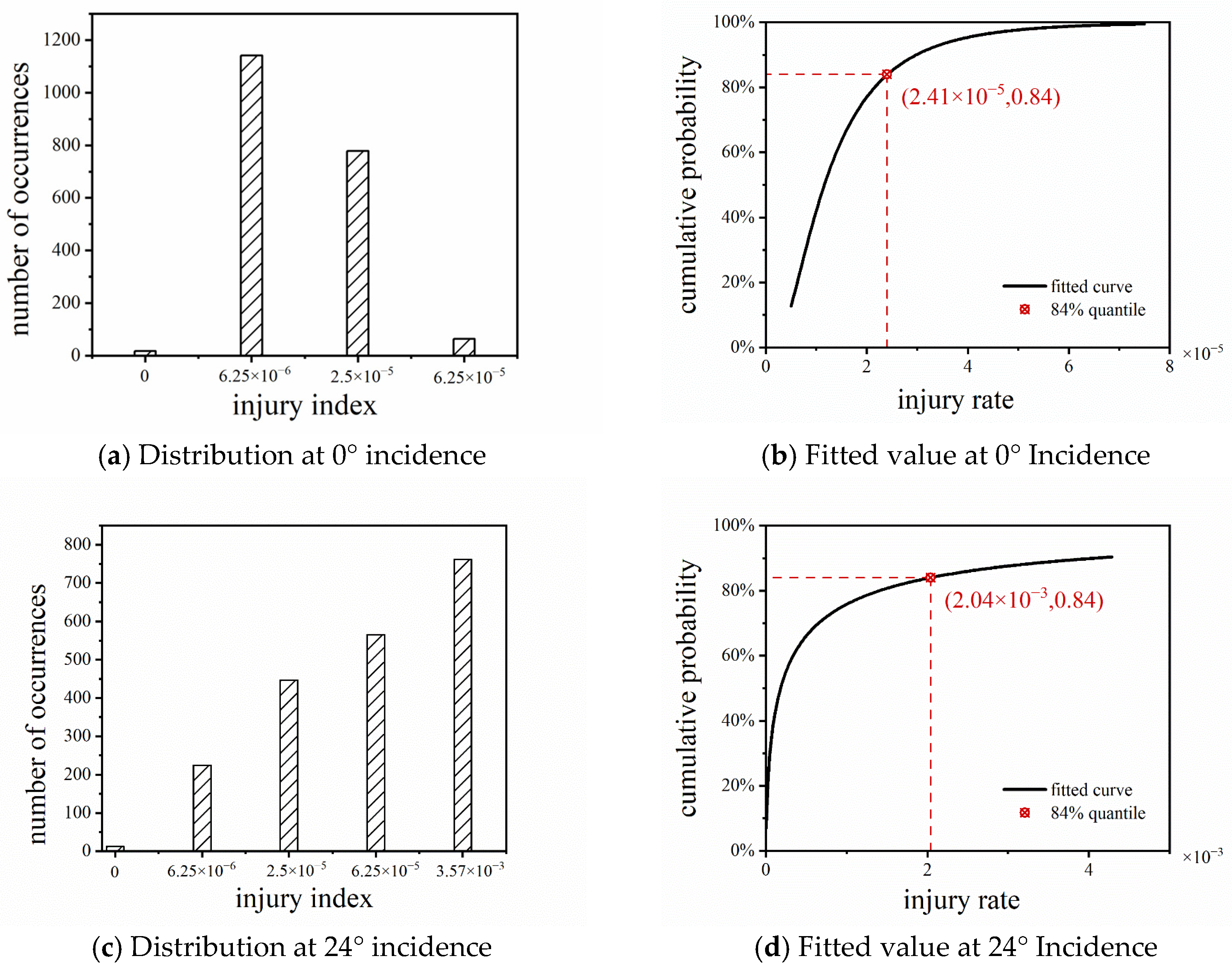
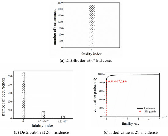
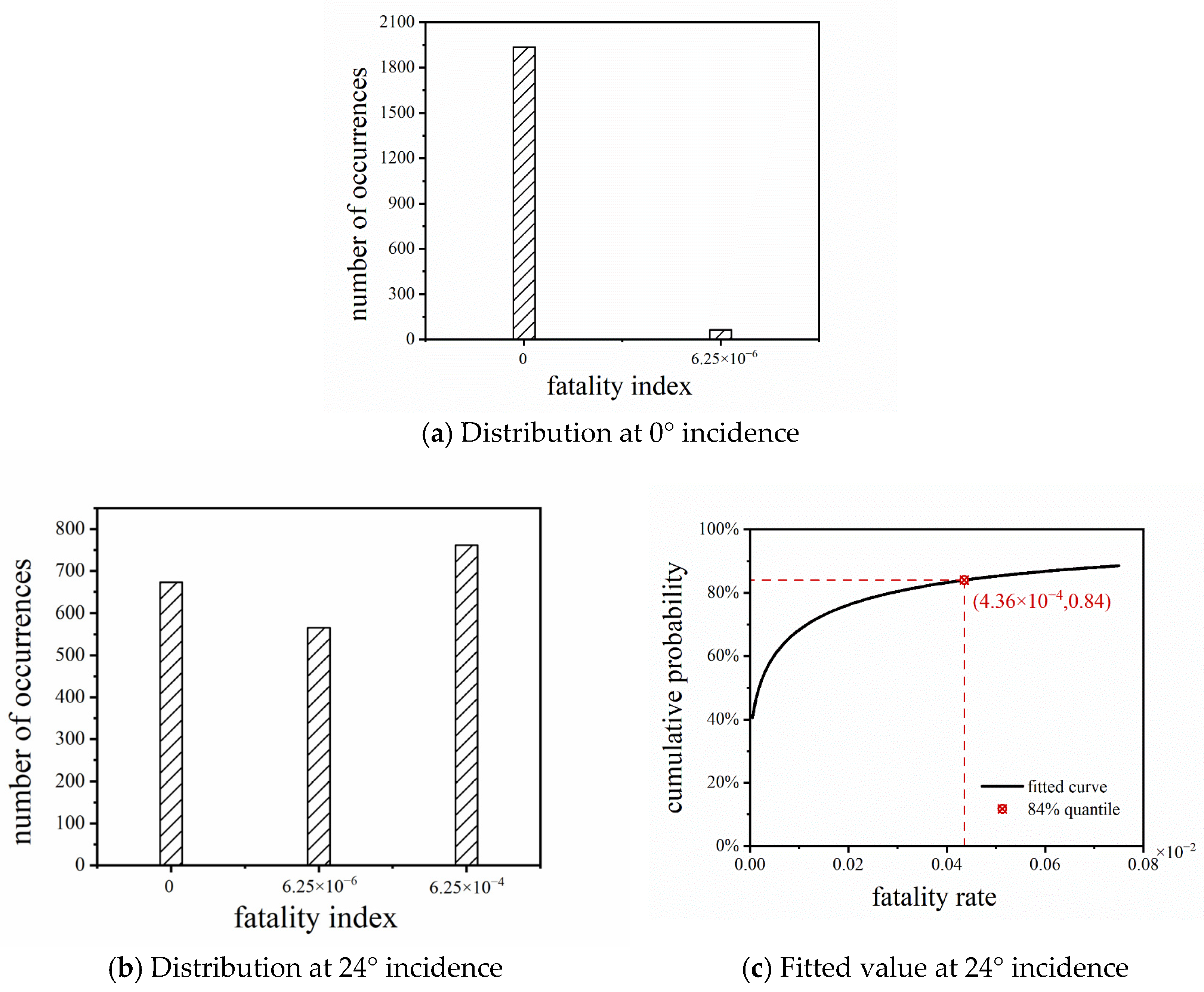
The distribution plots and fitted curves for the injury and fatality index under design basis earthquakes and the rare earthquakes are shown in Figure 28, Figure 29, Figure 30 and Figure 31.

Figure 28. Injury index under design basis earthquakes.

Figure 29. Injury index under rare earthquakes.

Figure 30. Fatality index under design basis earthquakes.

Figure 31. Fatality index under rare earthquakes.

Under design basis earthquakes, the injury index of the station is 8.99 × 10⁻⁶ at $\alpha$ = 0° and 8.09 × 10⁻⁵ at $\alpha$ = 24. Under the rare earthquake, the injury index is 2.41 × 10⁻⁵ at $\alpha$ = 0° and 2.04 × 10⁻³ at $\alpha$ = 24°.

Under the design basis earthquakes and the rare earthquakes, the proportions of zero values in the mortality rate distribution at 0° incidence are 100% and 96.8%, respectively. According to the zero-inflated lognormal distribution model, the zero portion is modeled using the empirical distribution; therefore, the fitted value corresponding to the 84th percentile of this indicator is 0. Under design basis earthquakes, the fatality index of the station is 0 at α = 0° and 9.61 × 10⁻⁸ at α = 24°. Under the rare earthquake, the fatality index is 0 at α = 0° and 4.36 × 10⁻⁴ at α = 24°.

4.5. Seismic Resilience Ratings

By comparing the fitted seismic resilience results with these criteria, the corresponding performance levels can be determined. Table 5 shows the ranges for each star rating of seismic resilience as specified in GB/T 38591–2020. Based on the fitted values and the rating criteria, the seismic resilience ratings for station structures under 0° and 24° incidence are presented in Table 6. The higher the star rating, the better the seismic resilience and the smaller the loss. Specifically, the three-star and two-star ratings are evaluated under the rare earthquake, whereas the one-star rating is evaluated under the design basis earthquake.

Table 5. Seismic-resilience star-rating criteria.

Resilience Rating	Seismic Level	Repair Cost Index $\mathit{\kappa }$	Repair Time Index T	Casualty Index
Three stars	rare	$\kappa$ ≤ 5%	T ≤ 7 d	${\gamma }_h$ ≤ 1.0 × 10−4, ${\gamma }_d$ ≤ 1.0 × 10−5
Two stars	rare	5% < $\kappa$ ≤ 10%	7 d < T≤ 30 d	${\gamma }_h$ ≤ 1.0 × 10−3, ${\gamma }_d$ ≤ 1.0 × 10−4
One star	design basis	$\kappa$ ≤ 10%	T ≤ 30 d	${\gamma }_h$ ≤ 1.0 × 10−3, ${\gamma }_d$ ≤ 1.0 × 10−4

Table 6. Summary of resilience indicators and star ratings under 0° and 24°.

	Repair Cost κ	Repair Time T	Injury ${\mathit{\gamma }}_{\mathit{h}}$	Fatality ${\mathit{\gamma }}_{\mathit{d}}$
α = 0° design basis	6.72%	7.27	8.99 × 10−6	0
Resilience rating	One star	One star	One star
α = 0° rare	11.88%	16.33	2.41 × 10−5	9.61 × 10−8
Resilience rating	—	Two stars	Three stars
α = 24° design basis	10.25%	11.29	8.09 × 10−5	0
Resilience rating	—	One star	One star
α = 24° rare	45.02%	49.23	2.04 × 10−3	4.36 × 10−4
Resilience rating	—	—	—

Where “—“indicates that the resilience rating required for this seismic level is not satisfied.

First, a check is performed to determine whether the one-star resilience rating under the design basis earthquake is satisfied. If this rating is achieved, further assessment is carried out to verify whether the two-star or three-star rating corresponding to the rare earthquake is also satisfied. Therefore, the final rating of the structure is presented in Table 7.

Table 7. Final rating of the station.

Incidence Angle	Repair Cost Index $\mathit{\kappa }$	Repair Time Index T	Casualty Index
0°	One star	Two stars	Three stars
24°	—	One star	One star

The lowest star rating among the three resilience indicators is taken as the overall seismic resilience rating of the structure. At $\alpha$ = 0°, the station is rated as one star in seismic resilience. At $\alpha$ = 24°, the overall rating decreases to below one star.

As the incidence angle increases from 0° to 24°, the repair cost, repair time, and casualties of the station structure all show significant increases. Under the design basis earthquake, the repair cost index and repair time index increase by 76% and 124%, respectively, and minor casualties occur. Under the rare earthquake, the resilience loss induced by oblique incidence at the near-critical angle is more pronounced: the repair cost and repair time increase by 339% and 336%, respectively, and severe casualties occur. Furthermore, the seismic resilience rating results indicate that when $\alpha$ = 24°, neither the design basis earthquake nor the rare earthquake satisfies the resilience rating requirements, demonstrating that near critical-angle incidence has a significant adverse impact on the seismic resilience of the station.

To investigate the variation in seismic resilience with incident angle, Figure 32 and Figure 33 present the curves of the fitted repair cost and fitted repair time versus incident angle, respectively.

Figure 32. Repair cost index versus incident angle.

Figure 33. Repair time index versus incident angle.

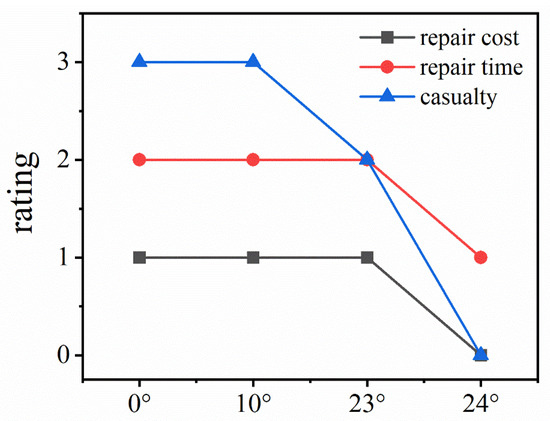
Overall, both indices exhibit a characteristic trend: an initial slight decrease, followed by a slow increase, and an abrupt change near the critical angle. In the range of 0° to 10°, both indices decrease. From 10° to 23°, they enter a phase of slow increase. As the incident angle reaches 24°, the index under the rare earthquake exhibits a pronounced increase, while those under the design-basis earthquake show a noticeable amplification. The casualty index follows a similar trend. The seismic resilience ratings of all resilience indices as a function of incident angle are shown in Figure 34 below:

Figure 34. Resilience ratings of all indices versus incident angle.

After incorporating the resilience evaluation results for α = 10° and α = 23° into the analysis, the variation in the structural resilience rating with incident angle exhibits clear nonlinear degradation characteristics. From α = 0° to α = 10°, the ratings of all three resilience indices remain unchanged, indicating that the structure maintains a favorable seismic resilience level throughout this angular range. When α increases to 23°, the casualty rating drops first from three stars to two stars, indicating a perceptible deterioration in occupant safety. Meanwhile, although the repair cost index and repair time index show a certain increase, their resilience ratings remain unchanged. When α reaches the near-critical angle of 24°, all ratings show an abrupt decrease. These results indicate that, near the critical angle, an extremely small deviation in incident angle can cause resilience to transition from partial degradation to severe loss.

These results indicate that resilience assessments derived from vertical incidence result in an overestimation of the seismic resilience of subway stations. Therefore, incorporating oblique incidence scenarios, particularly those near the critical angle, into the resilience assessment framework is of practical engineering significance.

5. Conclusions

This paper systematically investigates the influence of varying incidence angles on the rocking response, damage evolution, and seismic resilience of subway stations. The main conclusions are as follows:

(1)

At small-angle oblique SV-wave incidence, the subway station structure is dominated by shear deformation. As the incidence angle increases, the rocking response gradually becomes more pronounced, leading to a transition toward a shear–rocking coupled deformation mode. Near the critical angle, both the rocking angle and inter-story drift ratio increase sharply. This amplification effect is consistently observed across 11 ground motion records.

(2)

At vertical incidence, damage to the central column is concentrated at the column ends and is primarily tensile. At near-critical-angle, the rocking angle and inter-story drift ratio increase sharply, resulting in severe tensile damage developing along the column. The compressive damage to the concrete at the column ends is more severe. The column’s damage pattern becomes consistent with localized compression–shear damage, resulting in a significant degradation in the central column’s lateral stiffness.

(3)

Compared with vertical incidence, the overall seismic resilience deteriorates significantly under near-critical-angle oblique incidence, with the resilience rating decreasing from one star to below one star. The repair cost, repair time, and life-safety performance all show a significant degradation, leading to lower corresponding ratings. These results indicate that resilience assessments derived from vertical incidence result in an overestimation of the seismic resilience of subway stations.

(4)

Even a slight deviation at near-critical angle can cause significant changes in the structural response. The oblique SV-wave incidence at near critical-angle is a key factor that should be considered in seismic resilience assessment. The consideration of the critical angle of obliquely incident SV waves is of significant engineering importance for seismic resilience assessment.

References

- Hashash, Y.M.A.; Hook, J.J.; Schmidt, B.; Yao, J.I.C. Seismic design and analysis of underground structures. Tunn. Undergr. Space Technol. 2001, 16, 247–293. [Google Scholar] [CrossRef] [Scilit]
- An, X.H.; Shawky, A.A.; Maekawa, K. The collapse mechanism of a subway station during the Great Hanshin earthquake. Cem. Concr. Compos. 1997, 19, 241–257. [Google Scholar] [CrossRef] [Scilit]
- Takagi, J.; Wada, A. Recent earthquakes and the need for a new philosophy for earthquake-resistant design. Soil Dyn. Earthq. Eng. 2019, 119, 499–507. [Google Scholar] [CrossRef] [Scilit]
- Li, L.Y.; Chang-Richards, A.; Boston, M. Post-disaster functional recovery of the built environment: A systematic review and directions for future research. Int. J. Disaster Risk Reduct. 2023, 95, 103899. [Google Scholar] [CrossRef] [Scilit]
- Iida, H.; Hiroto, T.; Yoshida, N.; Iwafuji, M. Damage to Daikai Subway Station. Soils Found. 1996, 36, 283–300. [Google Scholar] [CrossRef] [Scilit] [PubMed]
- Hu, J.; Wen, W.; Zhai, C.; Wang, T.; Xie, L. A comprehensive review of resilience of urban metro systems: A perspective from earthquake engineering. Tunn. Undergr. Space Technol. 2024, 152, 105920. [Google Scholar] [CrossRef] [Scilit]
- Ma, C.; Zhao, Y.Q.; Wang, H.; Ren, J.J.; Wang, X.; Chen, M. Development of seismic resilience index and assessing framework of underground frame structures based on economic loss. Soil Dyn. Earthq. Eng. 2025, 194, 109373. [Google Scholar] [CrossRef] [Scilit]
- Yan, Y. Review of earthquake resistance and mitigation of underground structures. Adv. Res. 2024, 25, 156–162. [Google Scholar] [CrossRef] [Scilit]
- Holling, C.S. Resilience and stability of ecological systems. Annu. Rev. Ecol. Syst. 1973, 4, 1–23. [Google Scholar] [CrossRef] [Scilit]
- Almufti, I.; Willford, M. REDi Rating System: Resilience-Based Earthquake Design Initiative for the Next Generation of Buildings; Arup: London, UK, 2013. [Google Scholar]
- Bruneau, M.; Chang, S.E.; Eguchi, R.T.; Lee, G.C.; O’Rourke, T.D.; Reinhorn, A.M.; Shinozuka, M.; Tierney, K.; Wallace, W.A.; von Winterfeldt, D. A framework to quantitatively assess and enhance the seismic resilience of communities. Earthq. Spectra 2003, 19, 733–752. [Google Scholar] [CrossRef] [Scilit]
- Cimellaro, G.P.; Reinhorn, A.M.; Bruneau, M. Framework for analytical quantification of disaster resilience. Eng. Struct. 2010, 32, 3639–3649. [Google Scholar] [CrossRef] [Scilit]
- Lin, P.H.; Wang, N.Y.; Ellingwood, B.R. A risk de-aggregation framework that relates community resilience goals to building performance objectives. Sustain. Resilient Infrastruct. 2016, 1, 1–13. [Google Scholar] [CrossRef] [Scilit]
- Yang, F.; Zhuang, H.Y.; Yun, L.; Wang, D.P.; Xu, Z.G. Seismic resilience assessment method of underground subway station and verification study on Daikai station. J. Vib. Eng. 2025. (In Chinese) [Google Scholar] [CrossRef]
- Yang, F.; Zhuang, H.Y.; Yun, L.; Wang, D.P.; Xu, Z.G. Evaluation method for seismic resilience of underground structures and its verification. Soil Dyn. Earthq. Eng. 2010, 200, 109826. [Google Scholar]
- Wang, T.; Zhang, X.; Yang, S.; Shahzad, M.M. Quantifying the influence of modeling uncertainties on performance evaluation of mega column-core tube-outrigger structure under near-field and far-field ground motions. J. Build. Eng. 2022, 59, 105052. [Google Scholar] [CrossRef] [Scilit]
- Shahzad, M.M.; Zhang, X.; Wang, X.; Abdulhadi, M. Comparative response assessment of different steel plate shear walls (SPSWs) under near-field ground motion. J. Constr. Steel Res. 2022, 190, 107147. [Google Scholar] [CrossRef] [Scilit]
- Shahzad, M.M.; Zhang, X.; Wang, X.; Abdulhadi, M.; Wang, T.; Xiao, Y. Response control analysis of a new mega-subcontrolled structural system (MSCSS) under seismic excitation. Struct. Des. Tall Spec. Build. 2022, 31, e1935. [Google Scholar] [CrossRef] [Scilit]
- Xue, Y.; Li, X.; Wang, L.; Liu, Y.; Cao, X.; Zhang, Y. Mesoscopic damage enhancement in granite under cyclic liquid nitrogen shocks characterized by computed tomography and texture analysis. Int. J. Rock Mech. Min. Sci. 2025, 194, 106217. [Google Scholar] [CrossRef] [Scilit]
- Li, X.; Xue, Y.; Dang, F.; Ranjith, P.G.; Xie, H.; Hou, P.; Cai, C. Microscale damage evolution of high-temperature granite under liquid nitrogen thermal shock based on computed tomography analysis. Eng. Geol. 2025, 356, 108274. [Google Scholar] [CrossRef] [Scilit]
- O’Rourke, M.J.; Bloom, M.C.; Dobry, R. Apparent propagation velocity of body waves. Earthq. Eng. Struct. Dyn. 1982, 10, 283–294. [Google Scholar] [CrossRef] [Scilit]
- Sun, B.B.; Shao, Y.Q.; Deng, M.J.; Xu, J. Stochastic seismic performance assessment of hydraulic tunnels considering oblique incoming P waves based on generalized probability density evolution method. Tunn. Undergr. Space Technol. 2025, 162, 106644. [Google Scholar] [CrossRef] [Scilit]
- Chen, L.; Zhang, L.J. A Seismic Wave Oblique Incidence Method and the Application in Gravity DAM Seismic Research. J. Earthq. Tsunami 2014, 8, 1450011. [Google Scholar] [CrossRef] [Scilit]
- Huang, J.Q.; Zhao, M.; Du, X.L. Non-linear seismic responses of tunnels within normal fault ground under obliquely incident P waves. Tunn. Undergr. Space Technol. 2017, 61, 26–39. [Google Scholar] [CrossRef] [Scilit]
- Lysmer, J.; Kuhlemeyer, R.L. Finite dynamic model for infinite media. J. Eng. Mech. Div. ASCE 1969, 95, 859–878. [Google Scholar] [CrossRef] [Scilit]
- Joyner, W.B.; Chen, A.T.F. Calculation of nonlinear ground response in earthquakes. Bull. Seismol. Soc. Am. 1975, 65, 1315–1336. [Google Scholar]
- Deeks, A.J.; Randolph, M.F. Axisymmetric time-domain transmitting boundaries. J. Eng. Mech. ASCE 1994, 120, 25–42. [Google Scholar] [CrossRef] [Scilit]
- Liu, J.B.; Du, Y.X.; Du, X.L.; Wang, Z.Y.; Wu, J. 3D viscous-spring artificial boundary in time domain. Earthq. Eng. Eng. Vib. 2006, 5, 93–102. [Google Scholar] [CrossRef] [Scilit]
- Zhao, M.; Du, X.L.; Liu, J.B. A high-order accurate artificial boundary condition: Out-of-plane exterior wave problem. Eng. Mech. 2012, 29, 7–14. (In Chinese) [Google Scholar]
- Huang, J.Q.; Du, X.L.; Zhao, M.; Wang, Y.F. A simplified seismic wave input method for near-field wave analysis. J. Vib. Shock 2015, 34, 77–82. (In Chinese) [Google Scholar]
- Bao, X.; Liu, J.B.; Li, S.T.; Wang, F.; Lu, X.H. Stability conditions of explicit integration algorithms when using 3D viscoelastic artificial boundaries. Earthq. Eng. Eng. Vib. 2022, 21, 929–945. [Google Scholar] [CrossRef] [Scilit]
- Wang, X.W.; Chen, J.T.; Xiao, M. Seismic responses of an underground powerhouse structure subjected to oblique incidence SV and P waves. Soil Dyn. Earthq. Eng. 2019, 119, 130–143. [Google Scholar] [CrossRef] [Scilit]
- Wang, H.Y.; Huang, D.L.; Wang, H.R. Seismic vulnerability analysis of utility tunnel with oblique incidence of SV waves based on IDA method in horizontal non-homogeneous field. Soil Dyn. Earthq. Eng. 2025, 197, 109537. [Google Scholar] [CrossRef] [Scilit]
- Zhu, H.; Yan, S.; Sun, W.; Liang, Y.; Wang, Z. Seismic response analysis of subway station under obliquely incident SV waves. Sci. Rep. 2024, 14, 11235. [Google Scholar] [CrossRef] [Scilit] [PubMed]
- Wang, Y.; Wu, M.; Yang, J. Nonlinear seismic analysis of subway station layered site under obliquely incident shear waves with arbitrary angles. Tunn. Undergr. Space Technol. 2025, 163, 105987. [Google Scholar] [CrossRef] [Scilit]
- Zhao, M.; Nie, Y.M.; Ding, Q.P.; Du, X.L.; Zhang, W.Y. Effects of oblique incidence of SV waves on seismic response and damage evolution of integrated underground-aboveground complexes. Eng. Fail. Anal. 2025, 174, 109500. [Google Scholar] [CrossRef] [Scilit]
- Qiu, D.; Chen, J.; Xu, Q. Dynamic responses and damage forms analysis of underground large-scale frame structures under oblique SV seismic waves. Soil Dyn. Earthq. Eng. 2019, 117, 216–220. [Google Scholar] [CrossRef] [Scilit]
- Xiong, G.; Wang, F.; Zhou, F. Torsional and rocking response analysis of foundations subjected to spatially inclined incident SV waves considering soil nonlinearity. Soil Dyn. Earthq. Eng. 2024, 184, 108868. [Google Scholar] [CrossRef] [Scilit]
- Zhou, F.; Xiang, W.; Wang, H.; Zhang, Z.; Zhou, Y. Torsional and rocking response of the foundation induced by obliquely spatial incident S waves. Soil Dyn. Earthq. Eng. 2020, 130, 105977.1–105977.11. [Google Scholar] [CrossRef] [Scilit]
- GB 50909—2014; Ministry of Housing and Urban-Rural Development of the People’s Republic of China. Code for Seismic Design of Urban Rail Transit Structures. China Planning Press: Beijing, China, 2014.
- Kuhlemeyer, R.L.; Lysmer, J. Finite element method accuracy for wave propagation problems. J. Soil Mech. Found. Div. ASCE 1973, 99, 421–427. [Google Scholar] [CrossRef] [Scilit]
- Jia, M.; Yu, K.; Qian, K. Measurement and visualization of crack patterns in basalt fabric reinforced fine-grained concrete with different textile structures using high-speed photography and a cohesive finite element model. Constr. Build. Mater. 2022, 349, 128785. [Google Scholar] [CrossRef] [Scilit]
- GB 50011—2010; Ministry of Housing and Urban-Rural Development of the People’s Republic of China. Code for Seismic Design of Buildings. China Architecture & Building Press: Beijing, China, 2010.
- GB/T 38591—2020; State Administration for Market Regulation of the People’s Republic of China, Standardization Administration of the People’s Republic of China. Standard for Seismic Resilience Assessment of Buildings. Standards Press of China: Beijing, China, 2020.
- Du, X.L.; Jiang, J.W.; El Naggar, M.H.; Xu, C.S.; Xu, Z.G. Inter-story drift ratio associated with performance objectives for shallow-buried multistory and span subway stations in inhomogeneous soil profiles. Earthq. Eng. Struct. Dyn. 2021, 50, 655–672. [Google Scholar] [CrossRef] [Scilit]
Disclaimer/Publisher’s Note: The statements, opinions and data contained in all publications are solely those of the individual author(s) and contributor(s) and not of MDPI and/or the editor(s). MDPI and/or the editor(s) disclaim responsibility for any injury to people or property resulting from any ideas, methods, instructions or products referred to in the content. |
© 2026 by the authors. Licensee MDPI, Basel, Switzerland. This article is an open access article distributed under the terms and conditions of the Creative Commons Attribution (CC BY) license.