AI-Driven Multi-Criteria Decision-Making Framework for Acoustic Performance Prediction and Optimization in Music Venue Design

Abstract

Music-venue acoustic design requires the simultaneous consideration of reverberation, clarity, definition, and sound distribution. This study developed an artificial intelligence (AI)-based prediction-to-decision framework integrating the Dynamic Beluga Whale Optimizer (DBWO), Light Gradient Boosting Machine (LightGBM), and Analytic Hierarchy Process (AHP). Wavelet-based impulse-response denoising and leakage-controlled predictor standardisation preceded four separate regression models for reverberation time estimated from a 30 dB decay (T30), early decay time (EDT), clarity index (C80), and definition index (D50). DBWO tuned the LightGBM hyperparameters, after which predicted physical values were converted into acoustically contextualised utility scores and combined using AHP weights. On the independent test venues, DBWO–LightGBM achieved lower prediction errors than the benchmark models across most acoustic indicators and frequency bands. The balanced reflection–absorption alternative ranked first, and the ranking remained stable under AHP weight-sensitivity analysis. The framework therefore provides transparent decision support for predefined acoustic alternatives without claiming to generate venue geometry or replace detailed acoustic simulation.

1. Introduction

Music-venue acoustic quality is evaluated through measurable room-acoustic parameters, including reverberation time, early decay time, clarity, definition, and spatial sound distribution, under frequency- and position-dependent conditions [1,2]. Architectural acoustics requires the coordinated interpretation of measurement, simulation, spatial configuration, material behaviour, and occupant-related conditions because room-acoustic performance cannot be represented adequately by a single indicator or isolated design variable [3]. Artificial intelligence (AI) can support acoustic design evaluation, and geometry-plus-impulse-response datasets can support machine-learning research in acoustics [4,5]. Because material properties, sound reflection and absorption, diffusion, occupancy and source–receiver geometry interact, designers must compare several partly competing performance criteria rather than optimise a single indicator.

Performance-based acoustic design traditionally combines expert judgement, measurement and simulation. Multi-criteria decision-making (MCDM) has also been used in building ergonomics, retrofitting, envelope selection and site evaluation [6,7,8,9], while machine-learning surrogate models can accelerate the estimation of nonlinear building-performance relationships [4,10,11,12]. However, prediction alone does not establish the relative importance of competing acoustic goals or identify the most balanced alternative. A decision layer is therefore required to translate comparable acoustic evidence into transparent design priorities.

This study connects these functions in an acoustically contextualised framework. The Dynamic Beluga Whale Optimizer (DBWO) optimises Light Gradient Boosting Machine (LightGBM) hyperparameters for four independent acoustic regression models, whereas the Analytic Hierarchy Process (AHP) structures criterion priorities and ranks predefined design alternatives [13,14,15,16,17]. The approach distinguishes predictive-model optimisation from architectural-design optimisation: DBWO does not generate music-venue geometry, and AHP does not predict T30, EDT, C80, or D50.

However, conventional MCDM methods cannot be transferred mechanically across application domains, because their suitability depends on the structure of the decision problem, the nature of the criteria, and the preference information required for evaluation [13,14]. This limitation is particularly relevant to music-venue acoustics, where performance criteria differ in physical meaning and exhibit frequency- and space-dependent characteristics, while their design preferences do not necessarily follow a uniform “higher-is-better” or “lower-is-better” structure [1,2,18]. A generic weighting and ranking procedure may therefore overlook the physical meanings and design-specific requirements of acoustic indicators. The framework proposed in this study addresses this boundary by embedding acoustically informed criterion definitions and preference structures within a data-driven multi-criteria decision process. This domain-specific adaptation distinguishes the framework from a direct application of conventional MCDM and strengthens the necessity and originality of the study.

In this study, acoustic performance prediction refers to the data-driven estimation of objective room-acoustic parameters used to characterise the performance of a music venue, whereas an AI-driven multi-criteria decision-making framework refers to a decision-support structure that connects machine-learning-based performance estimation with structured multi-criteria evaluation [4,13]. Within this framework, DBWO–LightGBM denotes the predictive component in which the Dynamic Beluga Whale Optimizer supports the optimisation of LightGBM hyperparameters, while AHP constitutes the decision component that determines the relative priorities of the acoustic criteria and supports the comparison of predefined design alternatives [15,16]. Accordingly, optimisation in the present study encompasses predictive-model optimisation and the decision-oriented identification of a preferred alternative, rather than the automatic generation of music-venue geometry. The significance of the framework lies in addressing the disconnection between acoustic prediction and design decision-making: machine-learning models can estimate nonlinear acoustic performance but cannot independently determine the relative importance of competing design objectives, whereas MCDM methods can structure preferences and compare alternatives but require reliable performance information as their decision basis. By connecting these complementary functions, the study extends data-driven acoustic analysis from performance estimation to structured and interpretable design support. Its contribution to the existing body of knowledge therefore lies not merely in combining DBWO, LightGBM, and AHP, but in establishing a coherent prediction–evaluation linkage for multi-criteria decision-making in music-venue acoustics.

This study makes three contributions. First, it establishes a continuous prediction-to-decision framework for music-venue acoustics. Second, it uses DBWO–LightGBM to generate outcome-specific acoustic predictions under grouped venue-level validation. Third, it translates predicted physical values into acoustically meaningful utilities and an interpretable AHP ranking for early-stage design screening [17].

2. Related Works

2.1. Acoustic Performance Evaluation in Music Venue Design

Acoustic optimisation of concert halls and other music spaces requires the simultaneous evaluation of multiple acoustic indicators and design constraints. Attributes of sound in a performance space include reverberation, clarity, definition, spatial distribution, audience density, and material properties. These factors are interdependent and may produce competing acoustic outcomes. An intervention that increases perceived musical warmth may not simultaneously improve articulation, definition or spatial uniformity. Music-venue design should therefore be viewed as a multi-criteria decision-making problem rather than a single-objective optimisation problem. Diffusive design can alter objective parameters and perceived acoustic quality, so diffusion should be evaluated within a multi-parameter sound field [19]. Performer occupancy introduces additional absorption and can change audience-area acoustic conditions [20].

The main elements of music venue performance are sound clarity, reverberation, and the experience of the audience, and construction conditions such as surface materials, spatial forms, and occupancy affect acoustic results. Computational intelligence and multi-criteria decision-making (MCDM) can therefore be applied to compare sound-absorbing materials and support design-oriented selection. Although many previous studies have been conducted on the acoustics of the system or its general decision-making methods, few have integrated acoustic prediction with structured multi-criteria optimisation. Auditorium simulations also show that surface-scattering assumptions affect reverberation, early-decay, and definition-related outcomes [21]. Stage measurements and listening experiments further indicate that source–receiver directivity and the timing, direction, diffusivity, and strength of early reflections affect acoustic conditions [22,23].

2.2. Machine Learning for Acoustic Prediction

Machine-learning surrogate models approximate complex nonlinear relationships between design inputs and performance outputs and can therefore support rapid comparison when repeated high-fidelity simulation is impractical [4,10,11,12,24]. Machine learning has become a broad data-driven paradigm in acoustics for learning complex relationships between acoustic observations and target outputs when representative data are available [25]. In room acoustics, this role is to estimate expected T30, EDT, C80, and D50 values from architectural, source–receiver, occupancy, and environmental predictors; it does not determine which acoustic objective is most important or which alternative should be selected [4,5,26].

LightGBM provides an efficient gradient-boosting implementation for structured data [27]. In the present framework, DBWO searches its hyperparameter space, while four separate regression models retain outcome-specific loss structures for T30, EDT, C80, and D50. The predicted values therefore become evidence for, rather than substitutes for, design judgement. Physics-informed deep learning provides a complementary direction by constraining room-impulse-response reconstruction with sound-propagation physics [28].

2.3. MCDM in Building Design

Building-related MCDM studies have addressed environmental ergonomics, seismic–energy retrofitting and renovation decision support [6,7,29].

Multi-criteria decision methods have been applied to building and construction projects because they can consider several different and sometimes conflicting factors simultaneously. Della Spina and Lanteri [30] investigated adaptive reuse options for an unused railway in Sicily through the Preference Ranking Organization Method for Enrichment Evaluations (PROMETHEE) within a collaborative decision-making system. Dürr et al. [31] developed the Construction Materials for Cities in a Climate Change model to help designers select wall, roof, and ground-surface materials using environmental, economic, and practical criteria. Pinzon Amorocho and Hartmann [32] proposed a residential-renovation framework using pairwise comparison and the Technique for Order Preference by Similarity to Ideal Solution (TOPSIS).

Other construction-management and building-performance studies have also used MCDM. García-Orozco et al. [33] found that AHP and TOPSIS are commonly used to rank customer demands within quality function deployment. Zhang and Esangbedo [34] combined the Compromise Ranking of Alternatives from Distance to Ideal Solution (CRADIS) with System-2 thinking for contractor selection and validated the ranking with the Weighted Sum Model (WSM) and TOPSIS. Moschetti et al. [35] evaluated the robustness of responsive building envelopes, while Sadrolodabaee et al. [36] used MCDM to assess recycled textile-reinforced cement façade cladding.

Collectively, these studies demonstrate that MCDM is suitable for building-design problems involving competing technical, environmental, and stakeholder criteria. The same logic is relevant to music-venue acoustics, where designers must balance acoustic performance, building constraints, material properties, audience experience, and practical feasibility. AHP was selected because it can organise acoustic criteria hierarchically, derive transparent priorities, and compare predefined alternatives.

2.4. Contextualisation of MCDM in Acoustics

Outside building design, one representative example combines user preferences with hybrid MCDM to improve service evaluation [37]. Such evidence demonstrates the portability of multi-criteria logic but does not justify transferring a generic ranking structure directly to music-venue acoustics.

Acoustic criteria have different physical meanings and preference directions: T30 and EDT are target-type measures, C80 and D50 are benefit-type measures within acceptable ranges, and SPL uniformity is represented by spatial variability [1,2,13,14,16,18]. Contextualisation therefore requires explicit criterion definitions, acoustically meaningful utility functions, and a transparent separation between prediction and decision.

2.5. Theoretical Basis and Proposition

Performance-based design evaluates architectural alternatives through measurable performance evidence rather than relying only on experience-based judgement. For music venues, the relevant evidence includes frequency-specific room-acoustic parameters and spatial sound-distribution measures [1,2,4].

Machine-learning surrogate modelling provides a rapid approximation of nonlinear acoustic relationships. It can answer what T30, EDT, C80, and D50 a specified alternative is expected to produce, but it cannot independently establish which acoustic target is more important or which alternative should be selected [4,5,10,11,12,24,27].

Multi-criteria decision theory supplies the complementary structure: AHP organises heterogeneous criteria, establishes relative priorities, distinguishes target-type from benefit-type preferences, converts physical predictions into comparable design utilities, and produces a transparent alternative ranking [13,14,16].

Theoretical Proposition.

The design-support value of AI-based acoustic prediction emerges when predicted acoustic evidence is embedded within an acoustically contextualised multi-criteria decision structure.

2.6. Research Gap and Problem Statement

Existing research has developed two largely separate methodological streams. The first applies machine learning to room-acoustic performance estimation, with primary emphasis on predictive accuracy and efficient acoustic assessment [4,26]. The second applies multi-criteria decision-making to building renovation, material selection, and building-performance evaluation, with emphasis on structuring criteria, assigning priorities, and ranking alternatives [32,35]. However, these streams remain insufficiently connected in the context of music-venue acoustics. Acoustic-prediction studies generally do not translate predicted performance into a structured comparison of design alternatives, whereas MCDM applications typically assume that reliable and comparable criterion values are already available. The specific scientific gap is therefore the absence of an acoustically contextualised prediction-to-decision framework that connects data-driven room-acoustic performance estimation with multi-criteria evaluation of music-venue design alternatives.

A corresponding practical gap exists in the design workflow. Architects, acoustic consultants, and building engineers must interpret multiple acoustic indicators that differ in physical meaning and may present competing design requirements. Although simulations and predictive models can provide quantitative performance information, these outputs do not independently determine the relative importance of the criteria or identify the most balanced design alternative. Consequently, the transition from acoustic analysis to design selection may continue to depend on fragmented interpretation, repeated simulation, and individual expert judgement rather than a transparent and reproducible multi-criteria process.

The present study addresses these gaps by integrating an optimised machine-learning prediction component with an acoustically structured decision component. DBWO–LightGBM provides data-driven estimates of key acoustic performance indicators, while AHP organises their relative priorities and supports the comparison of predefined acoustic design alternatives. The framework therefore converts predicted acoustic evidence into an interpretable decision structure rather than treating prediction and alternative evaluation as separate processes. In doing so, it extends machine-learning-based acoustic analysis towards design-oriented decision support and provides MCDM with acoustically meaningful performance information for alternative evaluation.

3. Methodology

3.1. Research Framework

The complete method followed five continuous steps: (1) establish venue-, source–receiver-, occupancy-, and frequency-specific acoustic records; (2) denoise the raw impulse responses and standardise the continuous predictors; (3) use DBWO to search for the optimal LightGBM hyperparameters; (4) predict T30, EDT, C80 and D50 with four separate regression models; and (5) convert predicted physical values into utilities and apply AHP weights to rank the predefined alternatives.

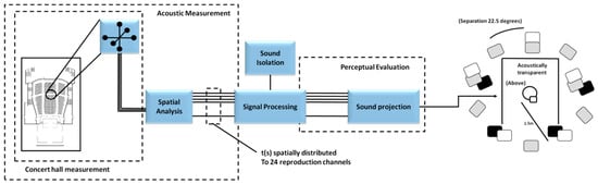
The methodological boundaries were explicit. DBWO optimised only LightGBM hyperparameters and did not generate concert-hall geometry. AHP evaluated and selected among predefined alternatives and did not predict acoustic indicators. Figure 1 situates the measurement and signal-processing basis for the framework.

Figure 1. Acoustic measurement and signal-processing workflow for music venue evaluation. Dashed boxes indicate the main workflow stages, arrows represent signal flow, and t(s) denotes the time-domain acoustic signal distributed across up to 24 reproduction channels.

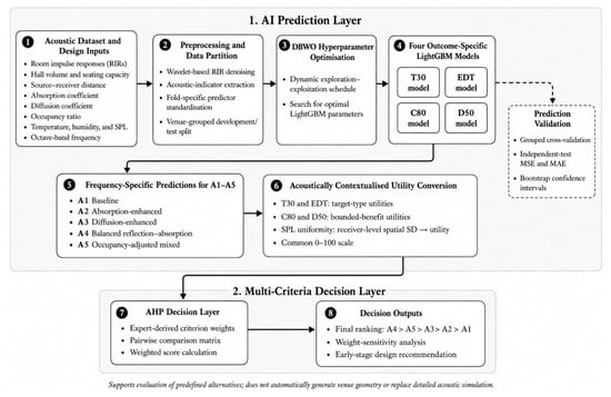
Figure 2 summarises the resulting prediction-to-decision chain from acoustic records through preprocessing, outcome-specific prediction, utility conversion, and alternative ranking.

Figure 2. Prediction-to-decision methodological framework. Solid arrows indicate the main sequential methodological and decision-making workflow, whereas the dashed arrow indicates the prediction-validation pathway.

3.2. Dataset and Sample Construction

The source acoustic records used in this study were obtained from the publicly available Concert Hall Acoustic Dataset hosted on Kaggle. The dataset is available at https://www.kaggle.com/datasets/ziya07/concert-hall-acoustic-dataset/data (accessed on 10 August 2026). The source records were subsequently organised into a balanced venue-level analytical structure for model development and independent testing. The resulting sample construction, predictor variables, acoustic outcomes, and data-partitioning procedure are described below.

The analytical structure comprised 18 music venues, with 20 source–receiver and occupancy configurations per venue, giving 360 base configurations. Each configuration was evaluated at the six octave-band centre frequencies of 125, 250, 500, 1000, 2000, and 4000 Hz, producing 2160 frequency-specific records. One analytical record represents one frequency-specific acoustic observation obtained from one music venue under a specified source–receiver, occupancy, and environmental configuration.

The balanced venue-level structure was selected to provide equal representation across the 18 venues and six octave-band frequencies. Assigning the same number of source–receiver and occupancy configurations to each venue prevented venues with denser observations from disproportionately influencing model fitting. The venue-level structure also preserved within-venue dependence while enabling grouped model validation and an independent evaluation of performance on previously unseen venues.

The model-development set contained 15 venues, 300 configurations, and 1800 records; the independent test set contained three venues, 60 configurations, and 360 records. Development-set validation used five grouped folds, with three venues per validation fold. Records from the same venue never appeared in both training and validation folds, and the three test venues remained unseen during training and hyperparameter optimisation.

The predictors were hall volume (mean: 15,420 m³, SD: 5180, range: 6200–24,800), seating capacity (1465 seats, SD: 540, range: 620–2480), source–receiver distance (19.7 m, SD: 8.2, range: 5.1–34.8), mean absorption coefficient (0.286, SD: 0.074, range: 0.150–0.450), diffusion coefficient (0.347, SD: 0.139, range: 0.100–0.600), occupancy ratio (0.642, SD: 0.216, range: 0.250–1.000), indoor temperature (22.1 °C, SD: 2.3, range: 18.0–26.0), relative humidity (52.4%, SD: 10.1, range: 35.1–69.8), sound-pressure level (77.2 dB, SD: 5.9, range: 65.0–89.9) and octave-band frequency. Each frequency contributed 360 records.

The outcomes were T30 (mean: 1.88 s, SD: 0.46, range: 0.82–3.12), EDT (1.71 s, SD: 0.43, range: 0.70–2.90), C80 (mean: 1.42 dB, SD: 2.37, range: −4.55–6.12) and D50 (mean: 63.7%, SD: 12.8, range: 27.6–91.0). Four independent regression models were fitted: Model 1 for T30, Model 2 for EDT, Model 3 for C80, and Model 4 for D50.

No missing predictor or outcome values remained in the analytical dataset; consequently, statistical imputation was not required.

3.3. Acoustic Signal and Data Preprocessing

Preprocessing comprised wavelet-based denoising of the room impulse responses and fold-specific standardisation of continuous predictors. Acoustic outcomes were derived after denoising and were not standardised.

3.3.1. Wavelet-Based Impulse-Response Denoising

Impulse responses were sampled at 48 kHz over a 6 s window. A five-level Daubechies-8 discrete wavelet transform was applied; noise was estimated by the median absolute deviation, the universal threshold was used with soft thresholding, and the signal was reconstructed by the inverse discrete wavelet transform before filtering into the 125–4000 Hz octave bands.

The purpose was to reduce the background-noise floor in the late impulse-response tail while retaining the direct-sound arrival, early reflections, and late-decay structure required for stable calculation of T30, EDT, C80, and D50.

3.3.2. Predictor Standardisation

Each continuous predictor was transformed using development-set statistics:

$$z_{ij}={\displaystyle \frac{x_{ij}-{\mu }_{j,train}}{{\sigma }_{j,train}}}$$

(1)

Here, $x_{ij}$ is the value of predictor $j$ for observation $i$, while ${\mu }_{j,train}$ and ${\sigma }_{j,train}$ are the mean and standard deviation estimated only from the relevant training data.

Standardisation was applied only to hall volume, seating capacity, source–receiver distance, absorption, diffusion, occupancy, temperature, humidity, and SPL. The categorical encoding of octave-band frequency and the T30, EDT, C80, and D50 outcomes were not standardised. Within grouped cross-validation, ${\mu }_{j,train}$ and ${\sigma }_{j,train}$ were estimated from each training fold and applied to its validation fold. The independent test set used parameters estimated from the complete development set, thereby preventing information leakage.

3.4. DBWO–LightGBM Prediction Models

3.4.1. LightGBM

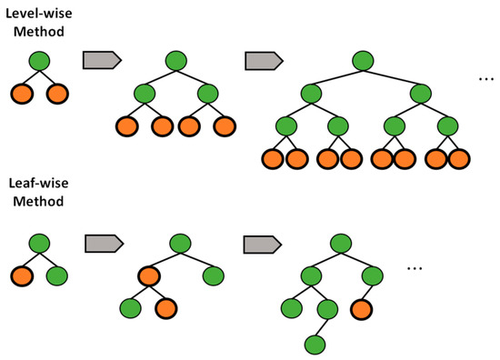
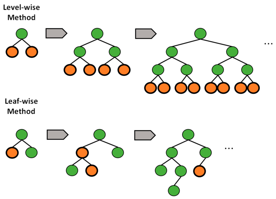
Light Gradient Boosting Machine is a gradient-boosted decision-tree algorithm designed for efficient modelling of structured data [27]. Its histogram-based feature discretisation reduces computational cost, while its leaf-wise growth strategy prioritises the leaf that produces the greatest reduction in the objective function. Because the present predictors were predominantly continuous numerical variables with nonlinear relationships and potential interaction effects, LightGBM provided a suitable balance between predictive flexibility and computational efficiency. Maximum depth, minimum leaf size, and regularisation parameters were constrained to reduce overfitting.

At boosting iteration t, the regularised objective is

$${\mathcal{L}}^{\left(t\right)}={\sum }_{i=1}^n\mathrm{l}\left(y_i,{\widehat{y}}_i^{(t-1)}+f_t\left(x_i\right)\right)+\Omega \left(f_t\right)$$

(2)

Here, $y_i$ is the observed value, ${\widehat{y}}_i^{(t-1)}$ is the prediction after t − 1 boosting iterations, $f_t\left(x_i\right)$ is the contribution of the t-th tree, $\mathrm{l}\left(·\right)$ is the regression loss, and $\Omega \left(f_t\right)$ penalises tree complexity.

Using a second-order Taylor approximation around the current prediction gives

$${\tilde{\mathcal{L}}}^{\left(t\right)}={\sum }_{i=1}^n\left[g_i{f}_t\left(x_i\right)+{\displaystyle \frac{1}{2}}{h}_i{f_t}^2\left(x_i\right)\right]+\Omega \left(f_t\right)$$

(3)

$$g_i={\displaystyle \frac{\partial \mathrm{l}\left(y_i,{\widehat{y}}_i\right)}{\partial {\widehat{y}}_i}},h_i={\displaystyle \frac{{\partial }^2\mathrm{l}\left(y_i,{\widehat{y}}_i\right)}{\partial {{\widehat{y}}_i}^2}}$$

(4)

The quantity $g_i$ is the first-order gradient and $h_i$ is the second-order Hessian of the loss with respect to the current prediction.

For the samples $I_j$ assigned to leaf $j$, the optimal leaf weight is

$${w_j}^{\ast }=-{\displaystyle \frac{{\sum }_{i\in I_j}{g}_i}{{\sum }_{i\in I_j}{h}_i+\lambda }}$$

(5)

In Equation (5), ${w_j}^{\ast }$ is the optimal score of leaf $j$, $I_j$ is its sample set, and $\lambda$ is the L2 regularisation coefficient.

The gain obtained by splitting a parent node into left and right children is

$$\mathrm{G}\mathrm{a}\mathrm{i}\mathrm{n}={\displaystyle \frac{1}{2}}\left[{\displaystyle \frac{{G_L}^2}{H_L+\lambda }}+{\displaystyle \frac{{G_R}^2}{H_R+\lambda }}-{\displaystyle \frac{{G_P}^2}{H_P+\lambda }}\right]-\gamma$$

(6)

Here, $G_L$ and $G_R$ are the sums of gradients in the left and right child nodes, $H_L$ and $H_R$ are the corresponding sums of Hessians, $G_P$ = $G_L$ + $G_R$ and $H_P$ = $H_L$ + $H_R$ are the parent-node sums, $\lambda$ regularises leaf weights, and $\gamma$ is the minimum split-gain penalty. Figure 3 contrasts the level-wise and leaf-wise tree-growth strategies.

Figure 3. Comparison of level-wise and leaf-wise tree-growth strategies. Green nodes indicate expanded or internal nodes, whereas orange nodes indicate terminal leaf nodes available for subsequent splitting.

3.4.2. Dynamic Beluga Whale Optimizer

The LightGBM search space combined continuous, integer, and discrete parameters with nonlinear interactions. Exhaustive grid search becomes costly as this space expands, whereas random search does not use information from previously evaluated candidate solutions. The original Beluga Whale Optimizer (BWO) provided population-based exploration, exploitation, and whale-fall position updates suitable for derivative-free search [15].

The dynamic BWO (DBWO) used the original BWO position-update operators within a transparent time-varying exploration–exploitation schedule. The probability of selecting the exploration update decreased linearly from 0.90 at the first iteration to 0.10 at the final iteration of the 80-iteration search process. For each candidate solution, the original BWO exploration update was applied when a uniformly distributed random number was lower than the corresponding exploration probability; otherwise, the original exploitation or whale-fall update was applied. After each update, continuous parameters were clipped to their predefined bounds, integer parameters were rounded before evaluation, and discrete parameters were decoded from their indexed categories. This time-varying exploration–exploitation schedule constituted the sole modification to the original BWO. Other BWO variants also refine search control [38].

3.4.3. Hyperparameter Search and Fitness Function

Each outcome-specific optimisation minimised the five-fold mean normalised root mean squared error (RMSE), so that the fitness remained a regression loss comparable across the four outcome scales:

$$\mathrm{F}\mathrm{i}\mathrm{t}\mathrm{n}\mathrm{e}\mathrm{s}\mathrm{s}\left(\theta \right)={\displaystyle \frac{1}{4}}{\displaystyle \sum _{k=1}^4}{\displaystyle \frac{{\mathrm{R}\mathrm{M}\mathrm{S}\mathrm{E}}_k\left(\theta \right)}{s_{y,k}}}$$

(7)

Here, $\theta$ is a candidate LightGBM hyperparameter vector, ${\mathrm{R}\mathrm{M}\mathrm{S}\mathrm{E}}_k\left(\theta \right)$ is the validation RMSE in grouped fold $k$, and $s_{y,k}$ is the training-fold standard deviation of the selected outcome.

The population size was 30, the maximum number of iterations was 80, and optimisation stopped after 10 consecutive iterations without improvement. Ten repeated optimisation runs were performed with five grouped folds and the fixed random seed 20260724.

The optimisation procedure began with 30 candidate hyperparameter vectors within the ranges in Table 1. Continuous values were clipped to their bounds, integer values were rounded, and discrete categories were decoded before evaluation. Each candidate was assessed using grouped five-fold normalised RMSE. The original BWO exploration, exploitation, and whale-fall updates [15] were applied using an exploration probability that decreased linearly from 0.90 to 0.10 over the 80-iteration search process. Parameter feasibility was enforced after every update, and the best feasible candidate was retained. Optimisation stopped after 80 iterations or 10 iterations without improvement, and the procedure was repeated 10 times. The candidate with the lowest fitness was then refitted on the complete development set and evaluated once on the independent test venues.

Table 1. Final hyperparameter solutions.

Hyperparameter	Search Range	T30	EDT	C80	D50
learning_rate	0.01–0.30	0.071	0.064	0.082	0.075
num_leaves	10–100	48	52	64	58
max_depth	3–15	8	8	10	9
min_data_in_leaf	5–50	14	13	11	12
feature_fraction	0.60–1.00	0.88	0.90	0.84	0.85
bagging_fraction	0.50–1.00	0.78	0.80	0.76	0.75
bagging_freq	0–10	5	4	5	5
lambda_l1	0–10	0.12	0.08	0.16	0.10
lambda_l2	0–10	0.63	0.55	0.72	0.50
max_bin	50–300	255	255	255	255
boosting rounds	100–1000	620	680	760	700

3.5. AHP Decision Layer and Utility Conversion

AHP organised the five heterogeneous criteria, derived their relative priorities from the 1–9 pairwise-comparison scale, and combined criterion utilities into an alternative score. It did not predict acoustic outcomes. T30 and EDT were treated as target-type criteria, C80 and D50 as benefit-type criteria within defined bounds, and SPL uniformity as a benefit associated with lower spatial variability.

Table 2 reports the criterion weights derived from the AHP comparison matrix. T30 received the largest weight (0.3047), followed by C80 (0.2485), D50 (0.1865), EDT (0.1620), and SPL uniformity (0.0983). T30 and EDT were interpreted as target-oriented criteria because values that deviate substantially in either direction from the design target may reduce acoustic suitability. C80 and D50 were treated as bounded benefit criteria, while SPL uniformity represented the consistency of sound distribution across receiver positions. The weights express the priorities of the decision scenario rather than universal acoustic laws.

Table 2. Acoustic criteria and their weight allocation.

Code	Criterion	Acoustic Meaning	Preference Direction	Weight
C1	T30/Reverberation time	Reverberation quality and musical fullness	Closer to design target is better	0.3047
C2	EDT/Early decay time	Perceived early decay and acoustic intimacy	Closer to design target is better	0.1620
C3	C80/Clarity	Musical clarity and articulation	Higher within acceptable range is better	0.2485
C4	D50/Definition	Sound definition and intelligibility	Higher within acceptable range is better	0.1865
C5	SPL uniformity	Uniformity of sound distribution across seating zones	Higher utility score is better	0.0983

The pairwise comparison judgments were obtained from a purposively selected panel of seven experts, comprising three university researchers specialising in architectural or room acoustics, two practising acoustic consultants or engineers, and two architects with experience in concert hall or music-venue design. Their relevant professional experience ranged from 8 to 21 years, with an average of approximately 13.6 years. All panel members had either conducted research on architectural acoustics or participated in at least one acoustic design, consultancy, or evaluation project involving a concert hall, theatre, or other music-performance venue. Before the assessment, the experts were provided with standardised definitions of T30, EDT, C80, D50, and SPL uniformity, together with instructions for applying Saaty’s 1–9 comparison scale. The experts initially completed the pairwise comparisons independently. A second-round consensus review was subsequently conducted for comparisons showing notable disagreement, and the final reciprocal judgments agreed upon by the panel were used to construct the comparison matrix presented in Table 3.

Table 3. Pairwise comparison matrix of acoustic criteria.

	C1 T30	C2 EDT	C3 C80	C4 D50	C5 SPL
C1 T30	1	2	1	2	3
C2 EDT	1/2	1	1/2	1	2
C3 C80	1	2	1	1	2
C4 D50	1/2	1	1	1	2
C5 SPL	1/3	1/2	1/2	1/2	1

Table 3 presents the final reciprocal comparison matrix developed from the expert assessments using Saaty’s 1–9 scale. The matrix represents the relative importance assigned to the five acoustic criteria and provides the basis for deriving their priority weights. The consistency of the pairwise comparison matrix was evaluated using the consistency index (CI) and consistency ratio (CR). For the five-criterion matrix, the maximum eigenvalue was λmax = 5.0713, resulting in CI = 0.0178. Using the random consistency index RI = 1.12 for a matrix of order five, the consistency ratio was calculated as CR = CI/RI = 0.0159. Since CR = 0.0159 < 0.10, the judgement matrix satisfied Saaty’s consistency criterion and was considered sufficiently consistent for deriving the criterion weights [16].

Table 4 interprets the weights reported in Table 2. T30 had the largest weight (0.3047), followed by C80 (0.2485), D50 (0.1865), EDT (0.1620), and SPL uniformity (0.0983). This ordering expresses the scenario-specific decision priorities without changing the physical meaning or preference direction of any criterion.

Table 4. Weights and ranking interpretation of acoustic criteria.

Criterion	Weight	Rank	Interpretation
T30	0.3047	1	Most important criterion because reverberation behaviour strongly shapes music venue sound quality.
C80	0.2485	2	Important for musical clarity and articulation.
D50	0.1865	3	Important for definition and intelligibility.
EDT	0.1620	4	Captures early decay and perceived acoustic intimacy.
SPL uniformity	0.0983	5	Supports balanced sound distribution across seating areas.

The utility anchors were defined for the medium-sized music-venue decision scenario examined in this study. T30 and EDT were treated as target-type criteria centred at 1.80 s and 1.60 s, respectively. C80 and D50 were treated as bounded benefit criteria over the intervals of −4 to 4 dB and 20% to 80%, while SPL spatial standard deviation was mapped from 0 to 5 dB. These anchors represent scenario-specific decision parameters rather than universal acoustic standards and should be recalibrated when the framework is applied to other venue types, performance genres, or occupancy conditions.

Six-band mean predictions were converted to 0–100 utilities using

$$U_{\mathrm{T}30}=100\mathrm{m}\mathrm{a}\mathrm{x}\left(0,1-{\displaystyle \frac{\left|\mathrm{T}30-1.80\right|}{1.00}}\right)$$

(8)

$$U_{\mathrm{E}\mathrm{D}\mathrm{T}}=100\mathrm{m}\mathrm{a}\mathrm{x}\left(0,1-{\displaystyle \frac{\left|\mathrm{E}\mathrm{D}\mathrm{T}-1.60\right|}{1.00}}\right)$$

(9)

$$U_{\mathrm{C}80}=100\mathrm{m}\mathrm{i}\mathrm{n}\left[1,\mathrm{m}\mathrm{a}\mathrm{x}\left(0,{\displaystyle \frac{\mathrm{C}80+4}{8}}\right)\right]$$

(10)

$$U_{\mathrm{D}50}=100\mathrm{m}\mathrm{i}\mathrm{n}\left[1,\mathrm{m}\mathrm{a}\mathrm{x}\left(0,{\displaystyle \frac{\mathrm{D}50-20}{60}}\right)\right]$$

(11)

$$U_{\mathrm{S}\mathrm{P}\mathrm{L}}=100\mathrm{m}\mathrm{a}\mathrm{x}\left(0,1-{\displaystyle \frac{{SD}_{\mathrm{S}\mathrm{P}\mathrm{L}}}{5}}\right)$$

(12)

The max and min operators clip all utilities to the 0–100 interval. SPL uniformity was not a fifth DBWO–LightGBM output. For each alternative $a$ and frequency $f$, it was calculated independently across $R$ = 20 receiver positions:

$${SD}_{a,f}=\sqrt{{\displaystyle \frac{1}{R-1}}{\sum }_{r=1}^R{\left({\mathrm{S}\mathrm{P}\mathrm{L}}_{a,f,r}-{\overline{\mathrm{S}\mathrm{P}\mathrm{L}}}_{a,f}\right)}^2}$$

(13)

In Equation (13), a denotes the alternative, $f$ the octave band, $r$ the receiver position, $R$ the number of receiver positions, and ${\overline{\mathrm{S}\mathrm{P}\mathrm{L}}}_{a,f}$ their mean SPL.

For the A1–A5 comparison, hall volume was fixed at 15,000 m³, seating capacity at 1500, source–receiver distance at 20 m, temperature at 22 °C, relative humidity at 50%, and reference SPL at 78 dB. Only the numerical conditions in Table 5 varied across alternatives.

Table 5. Numerical input conditions for acoustic design alternatives.

Alternative	Absorption Coefficient	Diffusion Coefficient	Occupancy Ratio	Other Conditions
A1 Baseline	0.24	0.28	0.60	Baseline
A2 Absorption-enhanced	0.38	0.28	0.60	Higher absorption
A3 Diffusion-enhanced	0.24	0.50	0.60	Higher diffusion
A4 Balanced reflection–absorption	0.34	0.44	0.60	Balanced intervention
A5 Occupancy-adjusted mixed	0.32	0.42	0.90	High-occupancy condition

3.6. Model Training and Validation

All analyses were conducted in Python 3.10.13. The analytical environment included LightGBM 4.5.0, CatBoost 1.2.7, scikit-learn 1.5.2, TensorFlow 2.16.1, PyWavelets 1.7.0, NumPy 1.26.4, and pandas 2.2.3. Computation was performed on a Windows 11 workstation equipped with an Intel Core i7 processor and 16 GB of RAM. The random seed was fixed at 20260724 for data partitioning, model initialisation, and repeated optimisation.

All models used the same predictors, development venues, independent test venues, outcomes, and preprocessing logic. The deep neural network (DNN) comprised hidden layers of 128, 64, and 32 units with rectified linear unit (ReLU) activation, a 0.20 dropout, Adam optimisation, a 0.001 learning rate, a batch size of 32, a maximum of 300 epochs, and early-stopping patience of 20. CatBoost used 700 iterations, a depth of 8, a 0.05 learning rate, L2 leaf regularisation of 3, and RMSE loss.

Model error was evaluated as mean squared error (MSE) and mean absolute error (MAE) on the independent test venues. The ablation comparison included standard LightGBM, random-search LightGBM, original BWO–LightGBM, and DBWO–LightGBM, alongside DNN and CatBoost.

The ablation sequence showed incremental improvement from standard LightGBM to random-search LightGBM, original BWO–LightGBM, and DBWO–LightGBM. The reductions were moderate rather than disruptive, supporting the interpretation that the dynamic modifications primarily improved search stability and hyperparameter refinement.

Prediction uncertainty was examined using 1000 configuration-level bootstrap resamples of the independent test set. Each source–receiver and occupancy configuration was treated as one resampling cluster, and its six octave-band records were retained together. The 2.5th and 97.5th percentiles of the bootstrap distributions were used as 95% confidence limits for MSE and MAE.

3.7. Sensitivity and Robustness Analysis

Ranking robustness was assessed with 10,000 AHP weight perturbations. Each baseline weight varied independently within ±20%, after which the five weights were renormalised to sum to one, and the alternative scores were recalculated. This analysis evaluated the stability of the A4–A5 decision under plausible changes in the scenario-specific priorities. MCDM sensitivity analysis tested whether rankings depend on criterion weights [39].

4. Results

4.1. Dataset Characteristics and Preprocessing Results

The final dataset contained 2160 complete frequency-specific records: 1800 from the 15 development venues and 360 from the three independent test venues. Each of the six octave bands contained 360 records, and no statistical imputation was required.

Wavelet denoising increased the signal-to-noise ratio from 24.8 ± 4.1 dB to 34.6 ± 3.7 dB. The early-response waveform correlation after processing was 0.982 ± 0.011. The median direct-arrival displacement was 0 samples, and the maximum displacement was two samples (0.042 ms). The noise floor was therefore substantially reduced while the timing structure required for T30, EDT, C80 and D50 remained effectively unchanged.

4.2. Prediction Performance

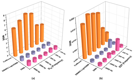
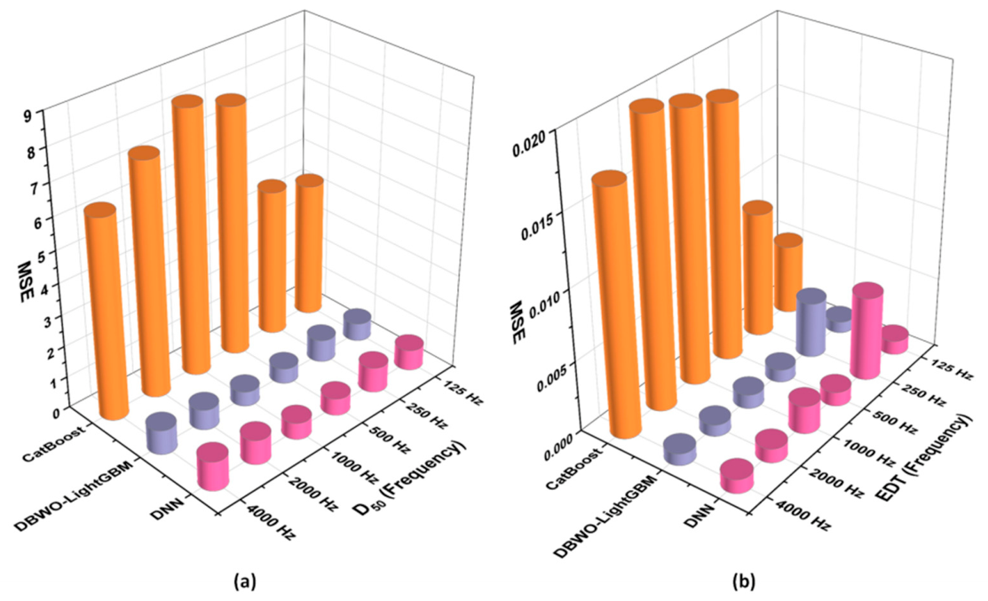
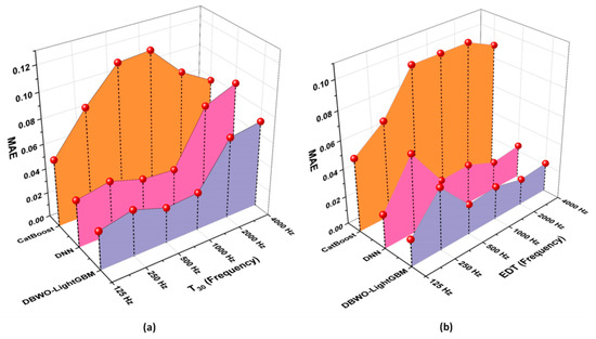
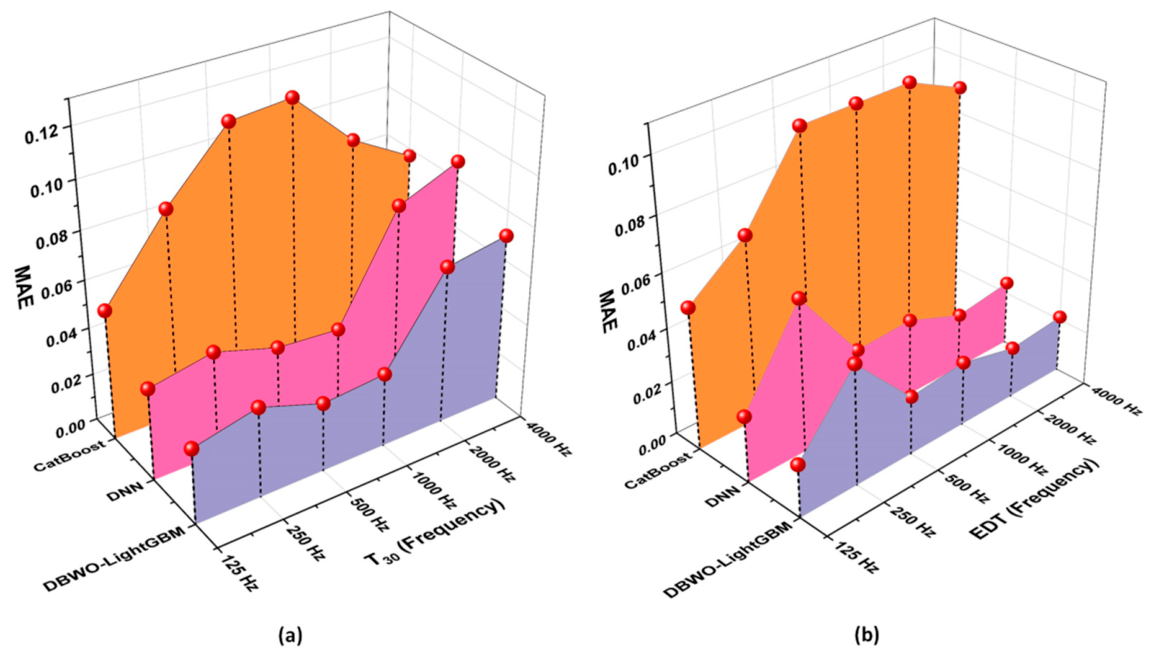
The four regression tasks were evaluated with MSE and MAE on the independent test venues. Table 6 shows the frequency-averaged ablation and benchmark comparison, while Table 7 and Table 8 report frequency-specific errors. The frequency-specific error patterns are also visualised in Figure 4 and Figure 5.

Table 6. Frequency-averaged MAE in the ablation and benchmark comparison.

Model	T30	EDT	C80	D50
Standard LightGBM	0.0508	0.0294	0.3087	0.5964
Random-search LightGBM	0.0481	0.0281	0.2924	0.5781
Original BWO–LightGBM	0.0462	0.0265	0.2769	0.5528
DBWO–LightGBM	0.0443	0.0252	0.2647	0.5367
DNN	0.0528	0.0307	0.3350	0.6320
CatBoost	0.0897	0.0842	0.4053	1.9525

Bold values indicate the lowest MAE and thus the best performance in each column.

Table 7. Performance evaluation of MSE.

Indices	Frequency (Hz)	MSE
		DNN	CatBoost	DBWO–LightGBM
T30	125	0.006	0.006	0.005
	250	0.004	0.019	0.003
	500	0.006	0.037	0.005
	1000	0.005	0.036	0.004
	2000	0.020	0.019	0.015
	4000	0.019	0.013	0.012
C80	125	0.112	0.322	0.098
	250	0.082	0.312	0.075
	500	0.073	0.371	0.068
	1000	0.197	0.345	0.180
	2000	0.470	0.345	0.320
	4000	0.458	0.228	0.210
D50	125	0.659	4.293	0.580
	250	0.807	4.685	0.720
	500	0.541	7.851	0.490
	1000	0.529	8.324	0.470
	2000	0.784	7.387	0.650
	4000	0.933	6.325	0.780
EDT	125	0.001	0.005	0.00082
	250	0.006	0.009	0.004
	500	0.001	0.018	0.0009
	1000	0.002	0.019	0.0015
	2000	0.001	0.020	0.0012
	4000	0.001	0.017	0.0011

Table 8. Comparative analysis of MAE across models.

Indices	Frequency (Hz)	MAE
		DNN	CatBoost	DBWO–LightGBM
T30	125	0.039	0.055	0.032
	250	0.044	0.087	0.038
	500	0.036	0.113	0.029
	1000	0.034	0.115	0.031
	2000	0.077	0.091	0.066
	4000	0.087	0.077	0.070
C80	125	0.266	0.365	0.215
	250	0.228	0.354	0.197
	500	0.212	0.441	0.189
	1000	0.337	0.454	0.290
	2000	0.459	0.449	0.377
	4000	0.508	0.369	0.320
D50	125	0.625	1.549	0.498
	250	0.689	1.601	0.534
	500	0.567	2.180	0.490
	1000	0.573	2.235	0.498
	2000	0.625	2.175	0.570
	4000	0.713	1.975	0.630
EDT	125	0.025	0.053	0.020
	250	0.057	0.069	0.045
	500	0.028	0.098	0.022
	1000	0.029	0.098	0.024
	2000	0.021	0.098	0.019
	4000	0.024	0.089	0.021

Figure 4. MSE comparison for (a) D50 and (b) EDT.

Figure 5. MAE comparison for (a) T30 and (b) EDT.

DBWO–LightGBM produced the lowest MSE values for T30, C80, and D50 across all six octave-band frequencies. For EDT, DBWO–LightGBM achieved the lowest MSE at 125, 250, 500, and 1000 Hz, whereas DNN was marginally lower at 2000 and 4000 Hz. Averaged across frequencies, the MSE values of DBWO–LightGBM were 0.0073 for T30, 0.1585 for C80, 0.6150 for D50, and 0.00159 for EDT.

DBWO–LightGBM achieved the lowest MAE in all 24 indicator–frequency comparisons. Its frequency-averaged MAE values were 0.0443 for T30, 0.2647 for C80, 0.5367 for D50, and 0.0252 for EDT. The corresponding MAE ranges were 0.029–0.070 for T30, 0.189–0.377 for C80, 0.490–0.630 for D50, and 0.019–0.045 for EDT.

4.3. Alternative-Specific Acoustic Predictions and Utility Scores

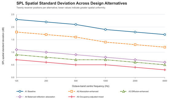
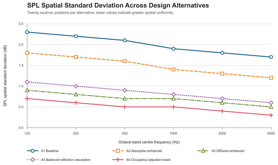
The numerical inputs in Table 5 were passed through the four fitted DBWO–LightGBM models at all six octave bands. Appendix A Table A1, Table A2, Table A3 and Table A4 report the frequency-specific predictions, while Table 9 reports their six-band means and the corresponding utilities. SPL spatial variability was calculated separately from 20 receiver positions per alternative. This receiver-level variation is summarised in Figure 6.

Table 9. Aggregated physical acoustic values and corresponding utility scores for each alternative.

Alternative	T30, s (Utility)	EDT, s (Utility)	C80, dB (Utility)	D50, % (Utility)	SPL Spatial SD, dB (Utility)
A1	2.15 (65)	1.98 (62)	0.64 (58)	53.0 (55)	2.00 (60)
A2	2.02 (78)	1.84 (76)	1.76 (72)	65.0 (75)	1.50 (70)
A3	1.98 (82)	1.80 (80)	2.72 (84)	66.8 (78)	0.70 (86)
A4	1.92 (88)	1.76 (84)	2.88 (86)	69.2 (82)	0.85 (83)
A5	1.96 (84)	1.72 (88)	2.40 (80)	71.6 (86)	0.50 (90)

Figure 6. Spatial standard deviation of SPL across receiver positions under the five design alternatives.

A1 had the lowest utilities across all five criteria. A4 obtained the strongest combination on the two highest-weighted criteria, T30 and C80, whereas A5 had the highest EDT, D50, and SPL-uniformity utilities. These values provide the explicit physical-to-utility linkage used in the final AHP calculation.

4.4. Final AHP Ranking

The final weighted score for alternative a was calculated as

$$S_a={\sum }_{j=1}^5{w}_j{U}_{a,j}$$

(14)

Here, $w_j$ is the AHP weight of criterion $j$ and $U_{a,j}$ is the corresponding utility for alternative a. Using Table 2 and Table 9, S_A4 = 0.3047(88) + 0.1620(84) + 0.2485(86) + 0.1865(82) + 0.0983(83) = 85.24.

Table 10 ranks A4 first (85.24), followed by A5 (84.62), A3 (81.82), A2 (74.84), and A1 (60.42). A4 was therefore the recommended alternative under the baseline weights, while the 0.62-point gap indicated that A5 remained a competitive alternative.

Table 10. Final AHP ranking result.

Rank	Alternative	Weighted Score	Decision Implication
1	A4 Balanced reflection–absorption	85.24	Recommended option; best overall balance across reverberation, clarity, definition, and early decay.
2	A5 Occupancy-adjusted mixed	84.62	Very close to A4; strongest in EDT, D50, and SPL uniformity.
3	A3 Diffusion-enhanced	81.82	Good spatial and clarity performance, but slightly weaker than A4 in T30 and D50.
4	A2 Absorption-enhanced	74.84	Improves over baseline but may not provide enough clarity/spatial balance.
5	A1 Baseline	60.42	Lowest overall score; should not be selected without further improvement.

4.5. Sensitivity Analysis

Across 10,000 renormalised ±20% weight perturbations, A4 retained first place in 99.5% of scenarios, and A5 ranked first in 0.5%. Although A4 and A5 were separated by only 0.62 points under the baseline weights, the perturbation results indicate that the ranking was highly stable within the tested ±20% weight range. The corresponding score distributions are reported in Table 11.

Table 11. Sensitivity analysis of alternative scores under AHP weight perturbations.

Alternative	Mean Score	2.5th Percentile	Median	97.5th Percentile	Ranked First
A1	60.42	60.01	60.42	60.82	0%
A2	74.84	74.55	74.84	75.12	0%
A3	81.82	81.59	81.82	82.04	0%
A4	85.24	85.00	85.25	85.48	99.5%
A5	84.62	84.31	84.61	84.93	0.5%

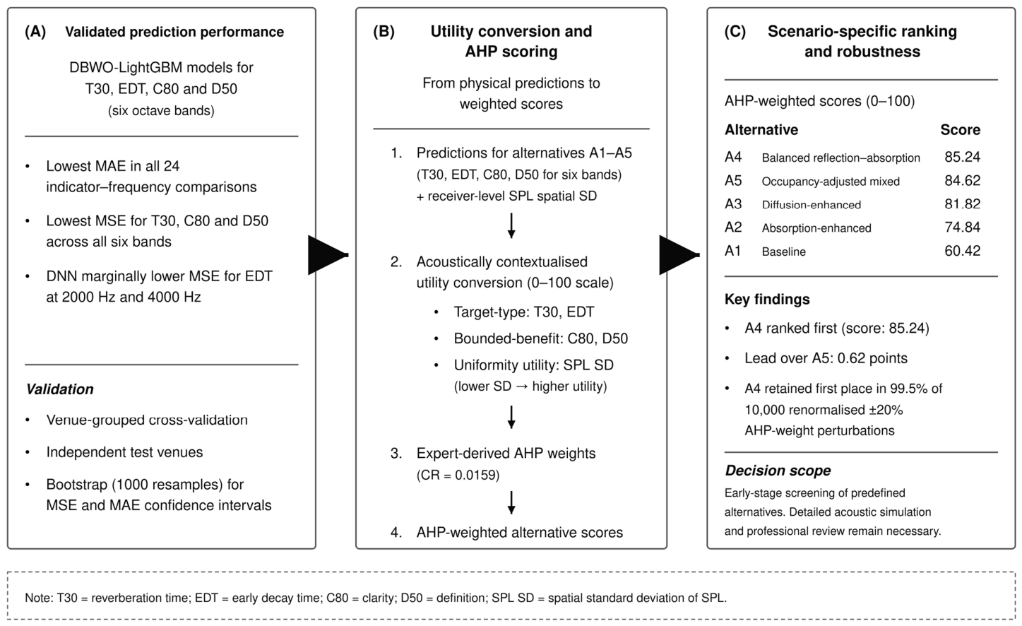
The bootstrap intervals were relatively narrow, indicating that the reported test-set errors were not driven by a small number of individual configurations. These intervals are reported in Table 12. Figure 7 presents the final AI-driven multi-criteria decision-making framework by integrating validated acoustic prediction, acoustically contextualised utility conversion, AHP-based evaluation, scenario-specific alternative ranking, and weight-sensitivity robustness.

Table 12. Configuration-level bootstrap confidence intervals for independent-test errors.

Outcome	MSE	95% CI	MAE	95% CI
T30	0.0073	0.0065–0.0082	0.0443	0.0411–0.0476
EDT	0.00159	0.00141–0.00179	0.0252	0.0235–0.0269
C80	0.1585	0.1462–0.1717	0.2647	0.2492–0.2805
D50	0.6150	0.5783–0.6551	0.5367	0.5096–0.5648

Figure 7. Final AI-driven multi-criteria decision-making framework for acoustic performance prediction and music-venue design support.

5. Discussion

5.1. Interpretation of Main Findings

Four findings define the main result. DBWO–LightGBM was the most stable overall predictor; DNN showed a local MSE advantage for EDT at 2000 and 4000 Hz; T30 and EDT were generally easier to predict than C80 and D50; and A4 remained the first-ranked alternative after AHP weighting and sensitivity analysis.

T30 and EDT are derived from decay behaviour, whereas C80 and D50 depend on the early-to-late energy partition. Local reflections, receiver position, and diffusion can therefore affect C80 and D50 more strongly than global architectural predictors capture. This finding is consistent with prior evidence showing sensitivity to source–receiver directivity, dominant early reflections, and diffuseness [19,21,22,23,40], as well as recent music-hall studies linking local geometry, surface scattering, and frequency-dependent absorption to differences among EDT, C80, and D50 [41,42]. The present study extends these findings by showing that this indicator-specific distinction remains visible at the level of machine-learning predictability under venue-grouped validation and independent testing on previously unseen venues.

The model comparison does not support an absolute-best claim in every condition. DNN produced marginally lower EDT MSE only at 2000 and 4000 Hz, and only for the MSE metric; DBWO–LightGBM nevertheless achieved the lowest MAE in all 24 indicator–frequency comparisons. The DNN result is therefore best interpreted as metric-specific and frequency-specific local variation, not as evidence of general high-frequency superiority or a reversal of the overall ranking. A cautious physical explanation is that high-frequency EDT is more sensitive to local reflections, surface properties, and source–receiver conditions, so different model structures may capture different residual patterns under those conditions [23,41,42].

The overall stability is broadly consistent with recent room-acoustic and building-performance studies showing that data-driven surrogate models can capture nonlinear relationships and interactions from structured representations during early design [43,44]. In the present data structure, this stability is plausible because the predictors were structured numerical variables and the acoustic outcomes depended on nonlinear relationships and interaction effects. The present study extends that evidence by retaining the performance pattern under venue-grouped validation and independent testing on previously unseen venues. Relative to the original BWO–LightGBM, DBWO–LightGBM reduced frequency-averaged MAE by approximately 4.1% for T30, 4.9% for EDT, 4.4% for C80, and 2.9% for D50. The principal predictive capacity still came from LightGBM and the training data; the dynamic exploration–exploitation schedule provided consistent but limited hyperparameter-search refinement. This task-specific increment does not establish universal superiority over other BWO variants or optimisation methods [15,38].

A4 and A5 reveal the compensatory logic of the decision layer. A4 was stronger on T30 and C80, which together accounted for 55.32% of the AHP weight, whereas A5 was stronger on EDT, D50, and SPL uniformity. A5’s higher-occupancy condition changed effective absorption and the spatial distribution of acoustic energy rather than functioning as a purely geometric intervention [20]. A4’s balanced absorption–diffusion setting is also acoustically plausible because scattering effects depend on surface location and surrounding absorption conditions [19,21]. Recent building MCDM research likewise treats the preferred alternative as a weighted compromise among competing criteria rather than one that must dominate every individual criterion [45,46]. This is the added value of the MCDM layer: AI predictions show how A1–A5 perform on each acoustic outcome, whereas AHP makes the criterion trade-offs explicit and yields a composite ranking. A4 should therefore be interpreted as the preferred alternative under the present scenario-specific utility anchors and AHP priorities, not as a universally optimal music-venue design.

A4 and A5 were separated by only 0.62 points, yet A4 ranked first in 99.5% of the tested ±20% weight perturbations. This result indicates that first place did not depend on one exact weight vector [39]. This result is consistent with recent MCDA research emphasising ranking persistence under plausible changes in criterion weights as an important indicator of decision robustness [47,48]. The ranking stability should nevertheless be interpreted as robustness to criterion-weight variation rather than as complete robustness to utility anchors, expert disagreement, prediction uncertainty or every other decision assumption.

5.2. Theoretical Implications

First, the framework establishes a prediction-to-decision linkage. Existing building and engineering-acoustic studies commonly emphasise either machine-learning prediction or optimisation and decision support [10,11,12,25,40,43,44]. The present structure connects physical prediction, acoustic utility, criterion weighting, and alternative ranking, so predictive evidence enters a transparent decision process rather than remaining an isolated accuracy result.

Second, the framework advances acoustically contextualised MCDM. T30 and EDT were represented as target-type criteria, C80 and D50 as bounded benefit-type criteria, and SPL uniformity as an inverse transformation of spatial variability. These distinctions prevent heterogeneous acoustic outcomes from being forced into a uniform min–max or higher-is-better rule [1,2,18,19,20,21,45,46].

Third, the framework clarifies methodological boundaries. AI predicts acoustic performance, DBWO optimises model hyperparameters, and AHP evaluates predefined alternatives; none of these components automatically generates venue geometry or replaces professional simulation. The contribution should therefore not be interpreted as evidence that data-driven prediction replaces acoustic physics; rather, the predictive model has a bounded evidential role within a broader decision process [25,28].

5.3. Practical Implications

The framework is intended for concept design and early option screening, when project teams need to compare technically feasible acoustic strategies before committing resources to detailed simulation and specification.

A practical workflow comprises five steps: (1) the project team proposes several technically feasible design alternatives; (2) each alternative is translated into the required acoustic, geometric, environmental and operational inputs; (3) the four outcome-specific models predict T30, EDT, C80 and D50; (4) project-appropriate utility anchors and AHP weights are defined; and (5) the highest-ranked alternatives proceed to detailed room-acoustic simulation, material design and professional review.

The framework is not a substitute for field measurement, high-fidelity room-acoustic simulation, material specification, or professional judgement. Its role is preliminary and transparent screening of predefined alternatives, not automatic geometry generation.

5.4. Limitations and Future Research

Data and external validity. The balanced dataset contained only 18 venues and cannot represent the full architectural, operational, and acoustic heterogeneity of music-performance spaces. External validation across venue types and real design projects is therefore required before practical deployment.

Model and feature limitations. The predictors did not encode complete three-dimensional geometry or explicit early-reflection paths, and no SHAP-based interpretability analysis was included. DBWO was not compared with a broader range of hyperparameter-optimisation approaches such as Bayesian optimisation. Future work could also test physics-informed representations that constrain data-driven sound-field estimates using acoustic propagation laws, particularly when measured room impulse responses are spatially sparse [28].

Decision-layer limitations. The analysis used one consensus AHP matrix and did not retain individual expert disagreement. The utility anchors were scenario-specific; equal averaging across six octave bands may not suit every musical genre or venue function, and A1–A5 were predefined alternatives. Future applications should test alternative elicitation procedures, genre-specific frequency priorities, and recalibrated utility anchors [39].

Uncertainty propagation. Configuration-level bootstrap intervals assessed prediction error, while the sensitivity analysis perturbed only criterion weights; neither step propagated predictive distributions through utility conversion to the final ranking. Future research should use Monte Carlo propagation of predictive uncertainty through utility conversion and multi-criteria scoring, jointly examining uncertainty in expert judgements, utility anchors, predicted criterion values and alternative-performance matrices [39].

5.5. Summary of Key Findings

DBWO–LightGBM provided the most stable overall prediction performance, achieving the lowest MAE across all 24 indicator–frequency comparisons, although DNN retained a local MSE advantage for EDT at 2000 and 4000 Hz. T30 and EDT were generally more predictable than C80 and D50, consistent with the greater local sensitivity of early-to-late energy measures. In the decision layer, A4 ranked first because its stronger T30 and C80 performance aligned with the two most heavily weighted criteria, whereas A5 performed better on several lower-weighted criteria. A4’s first-place position persisted in 99.5% of the ±20% weight-perturbation scenarios, indicating robustness to plausible criterion-weight changes while not implying universal robustness to other assumptions. Together, these findings support the final AI-driven multi-criteria decision-making framework: validated acoustic prediction supplies physical performance evidence, utility conversion makes heterogeneous outcomes comparable, AHP represents criterion priorities, and the combined scores produce a transparent scenario-specific ranking of predefined design alternatives. The evidence therefore links prediction, evaluation, and ranking without treating the preferred alternative as universally optimal or replacing detailed acoustic simulation.

6. Conclusions

This study developed an AI-driven prediction-to-decision framework that combined wavelet-based impulse-response denoising, leakage-controlled standardisation, four DBWO–LightGBM regression models, acoustically contextualised utility conversion and AHP ranking. DBWO–LightGBM achieved the lowest MAE in all 24 indicator–frequency comparisons and the lowest MSE for T30, C80 and D50 at every frequency, while DNN was marginally lower for EDT at the two highest frequencies.

The prediction outputs led to a transparent ranking of predefined alternatives: A4 ranked first with 85.24, narrowly ahead of A5 with 84.62, and remained first in 99.5% of the weight-sensitivity scenarios. The result supports the theoretical proposition that acoustic prediction becomes useful for design support when it is embedded in an acoustically contextualised multi-criteria decision structure. The framework is an early-stage screening aid and does not replace detailed simulation, measurement or professional judgement.

References

- ISO Standard No. 3382-1:2009; Acoustics—Measurement of Room Acoustic Parameters—Part 1: Performance Spaces. International Organization for Standardization: Geneva, Switzerland, 2009. Available online: https://www.iso.org/standard/40979.html (accessed on 10 August 2026).
- Yan, R.; Tronchin, L. Acoustic characteristics and objective evaluation of acoustic quality in historical Italian theaters. Appl. Acoust. 2025, 233, 110483. [Google Scholar] [CrossRef] [Scilit]
- Shtrepi, L.; Aletta, F.; Aspöck, L.; Astolfi, A.; Fels, J.; Hornikx, M.; Jambrošić, K.; Jeong, C.-H.; Kahle, E.; Llorca-Bofí, J.; et al. Ten questions concerning architectural acoustics. Build. Environ. 2024, 265, 112012. [Google Scholar] [CrossRef] [Scilit]
- Tabatabaei Manesh, M.; Nikkhah Dehnavi, A.; Tahsildoost, M.; Alambeigi, P. Acoustic design evaluation in educational buildings using artificial intelligence. Build. Environ. 2024, 261, 111695. [Google Scholar] [CrossRef] [Scilit]
- Xydis, A.; Perraudin, N.; Rust, R.; Heutschi, K.; Casas, G.; Riba Grognuz, O.; Eggenschwiler, K.; Kohler, M.; Perez-Cruz, F. GIR dataset: A geometry and real impulse response dataset for machine learning research in acoustics. Appl. Acoust. 2023, 208, 109333. [Google Scholar] [CrossRef] [Scilit]
- Serrano-Jiménez, A.; Díaz-López, C.; Ramírez-Juidias, E.; Barrios-Padura, Á. Multi-criteria assessment model on environmental ergonomics for decision-making in schoolyards based on remote-sensing and GIS resources. Sustain. Cities Soc. 2023, 92, 104481. [Google Scholar] [CrossRef] [Scilit]
- Caruso, M.; Pinho, R.; Bianchi, F.; Cavalieri, F.; Lemmo, M.T. Multi-criteria decision-making approach for optimal seismic/energy retrofitting of existing buildings. Earthq. Spectra 2023, 39, 191–217. [Google Scholar] [CrossRef] [Scilit]
- Ulutaş, A.; Balo, F.; Topal, A. A new hybrid MCDM method for optimizing natural stone selection for building envelopes. Rev. Construcción 2023, 22, 646–660. [Google Scholar] [CrossRef] [Scilit]
- Wahba, D.; Omran, A.A.; Adly, A.; Gad, A.; Arman, H.; El-Bagoury, H. Optimizing site selection for construction: Integrating GIS modeling, geophysical, geotechnical, and geomorphological data using the analytic hierarchy process. ISPRS Int. J. Geo-Inf. 2025, 14, 3. [Google Scholar] [CrossRef] [Scilit]
- Ali, A.; Jayaraman, R.; Mayyas, A.; Alaifan, B.; Azar, E. Machine learning as a surrogate to building performance simulation: Predicting energy consumption under different operational settings. Energy Build. 2023, 286, 112940. [Google Scholar] [CrossRef] [Scilit]
- D’Agostino, D.; De Falco, F.; Minelli, F.; Minichiello, F. New robust multi-criteria decision-making framework for thermal insulation of buildings under conflicting stakeholder interests. Appl. Energy 2024, 376, 124262. [Google Scholar] [CrossRef] [Scilit]
- Singh, M.M.; Deb, C.; Geyer, P. Early-stage design support combining machine learning and building information modelling. Autom. Constr. 2022, 136, 104147. [Google Scholar] [CrossRef] [Scilit]
- Cinelli, M.; Kadziński, M.; Miebs, G.; Gonzalez, M.; Słowiński, R. Recommending multiple criteria decision analysis methods with a new taxonomy-based decision support system. Eur. J. Oper. Res. 2022, 302, 633–651. [Google Scholar] [CrossRef] [Scilit]
- Greco, S.; Słowiński, R.; Wallenius, J. Fifty years of multiple criteria decision analysis: From classical methods to robust ordinal regression. Eur. J. Oper. Res. 2025, 323, 351–377. [Google Scholar] [CrossRef] [Scilit]
- Zhong, C.; Li, G.; Meng, Z. Beluga whale optimization: A novel nature-inspired metaheuristic algorithm. Knowl.-Based Syst. 2022, 251, 109215. [Google Scholar] [CrossRef] [Scilit]
- Saaty, T.L. The Analytic Hierarchy Process: Planning, Priority Setting, Resource Allocation; McGraw-Hill: Columbus, OH, USA, 1980. [Google Scholar]
- Abdel-Basset, M.; Gamal, A.; Chakrabortty, R.K.; Ryan, M.; El-Saber, N. A comprehensive framework for evaluating sustainable green building indicators under an uncertain environment. Sustainability 2021, 13, 6243. [Google Scholar] [CrossRef] [Scilit]
- Corrente, S.; Tasiou, M. A robust TOPSIS method for decision making problems with hierarchical and non-monotonic criteria. Expert Syst. Appl. 2023, 214, 119045. [Google Scholar] [CrossRef] [Scilit]
- Jeon, J.Y.; Jo, H.I.; Seo, R.; Kwak, K.H. Objective and subjective assessment of sound diffuseness in musical venues via computer simulations and a scale model. Build. Environ. 2020, 173, 106740. [Google Scholar] [CrossRef] [Scilit]
- Jeon, J.Y.; Jang, H.S.; Jo, H.I. Acoustic evaluation of orchestra occupancies in concert halls: Effect of sound absorption by orchestra members on audience acoustics. Build. Environ. 2018, 143, 349–357. [Google Scholar] [CrossRef] [Scilit]
- Zhu, X.; Xu, G.; Kang, J.; Xue, X.; Hao, Y. Influence of surface scattering on auditorium acoustic parameters. Buildings 2024, 14, 1882. [Google Scholar] [CrossRef] [Scilit]
- Wenmaekers, R.H.C.; Hak, C.C.J.M.; Hornikx, M.C.J.; Kohlrausch, A.G. Sensitivity of stage acoustic parameters to source and receiver directivity: Measurements on three stages and in two orchestra pits. Appl. Acoust. 2017, 123, 20–28. [Google Scholar] [CrossRef] [Scilit]
- Kriz, J.; Porcinai, E.; Lepa, S.; Klein, P.; Arend, J.M.; Weinzierl, S. How early reflections affect the stage acoustic conditions for solo musicians. Appl. Acoust. 2025, 235, 110644. [Google Scholar] [CrossRef] [Scilit]
- Shen, Y.; Pan, Y. BIM-supported automatic energy performance analysis for green building design using explainable machine learning and multi-objective optimization. Appl. Energy 2023, 333, 120575. [Google Scholar] [CrossRef] [Scilit]
- Bianco, M.J.; Gerstoft, P.; Traer, J.; Ozanich, E.; Roch, M.A.; Gannot, S.; Deledalle, C.-A. Machine learning in acoustics: Theory and applications. J. Acoust. Soc. Am. 2019, 146, 3590–3628. [Google Scholar] [CrossRef] [Scilit] [PubMed]
- Yu, Y.C.; Tsay, Y.S. Integrating parametric design and machine learning for room acoustics prediction in the early design stage of concert halls. Build. Acoust. 2026, 1351010X261456479. [Google Scholar] [CrossRef] [Scilit]
- Ke, G.; Meng, Q.; Finley, T.; Wang, T.; Chen, W.; Ma, W.; Ye, Q.; Liu, T.-Y. LightGBM: A highly efficient gradient boosting decision tree. Adv. Neural Inf. Process. Syst. 2017, 30, 3146–3154. Available online: https://proceedings.neurips.cc/paper_files/paper/2017/hash/6449f44a102fde848669bdd9eb6b76fa-Abstract.html (accessed on 10 August 2026).
- Karakonstantis, X.; Caviedes-Nozal, D.; Richard, A.; Fernandez-Grande, E. Room impulse response reconstruction with physics-informed deep learning. J. Acoust. Soc. Am. 2024, 155, 1048–1059. [Google Scholar] [CrossRef] [Scilit] [PubMed]
- Velykorusova, A.; Zavadskas, E.K.; Tupenaite, L.; Kanapeckiene, L.; Migilinskas, D.; Kutut, V.; Ubarte, I.; Abaravicius, Z.; Kaklauskas, A. Intelligent multi-criteria decision support for renovation solutions for a building based on emotion recognition by applying the COPRAS method and BIM integration. Appl. Sci. 2023, 13, 5453. [Google Scholar] [CrossRef] [Scilit]
- Della Spina, L.; Lanteri, C. A collaborative multi-criteria decision-making framework for the adaptive reuse design of disused railways. Land 2024, 13, 851. [Google Scholar] [CrossRef] [Scilit]
- Dürr, J.; Geissler, A.; Hoffmann, C. Development of a multi-criteria decision-making model to assist building designers in the choice of superficial construction systems in urban areas. J. Build. Phys. 2023, 46, 513–540. [Google Scholar] [CrossRef] [Scilit]
- Pinzon Amorocho, J.A.; Hartmann, T. A multi-criteria decision-making framework for residential building renovation using pairwise comparison and TOPSIS methods. J. Build. Eng. 2022, 53, 104596. [Google Scholar] [CrossRef] [Scilit]
- García-Orozco, S.; Vargas-Gutiérrez, G.; Ordóñez-Sánchez, S.; Silva, R. Using multi-criteria decision making in quality function deployment for offshore renewable energies. Energies 2023, 16, 6533. [Google Scholar] [CrossRef] [Scilit]
- Zhang, S.; Esangbedo, M.O. Urban scenic spot activity center investment: Strategic construction company selection using the grey System-II thinking compromise ranking of alternatives from distance to ideal solution multi-criteria decision-making method. Systems 2025, 13, 67. [Google Scholar] [CrossRef] [Scilit]
- Moschetti, R.; Homaei, S.; Taveres-Cachat, E.; Grynning, S. Assessing responsive building envelope designs through robustness-based multi-criteria decision making in zero-emission buildings. Energies 2022, 15, 1314. [Google Scholar] [CrossRef] [Scilit]
- Sadrolodabaee, P.; Hosseini, S.A.; Claramunt, J.; Ardanuy, M.; Haurie, L.; Lacasta, A.M.; de la Fuente, A. Experimental characterization of comfort performance parameters and multi-criteria sustainability assessment of recycled textile-reinforced cement facade cladding. J. Clean. Prod. 2022, 356, 131900. [Google Scholar] [CrossRef] [Scilit]
- Andreou, A.; Mavromoustakis, C.X.; Markakis, E.K.; Song, H. On the integration of user preferences by using a hybrid methodology for multi-criteria decision making. IEEE Access 2023, 11, 139157–139170. [Google Scholar] [CrossRef] [Scilit]
- Huang, J.; Hu, H. Hybrid beluga whale optimization algorithm with multi-strategy for functions and engineering optimization problems. J. Big Data 2024, 11, 3. [Google Scholar] [CrossRef] [Scilit]
- Demir, G.; Chatterjee, P.; Pamučar, D. Sensitivity analysis in multi-criteria decision making: A state-of-the-art research perspective using bibliometric analysis. Expert Syst. Appl. 2024, 237, 121660. [Google Scholar] [CrossRef] [Scilit]
- Wang, R.; Yao, D.; Zhang, J.; Xiao, X.; Jin, X. Sound-insulation prediction model and multi-parameter optimisation design of the composite floor of a high-speed train based on machine learning. Mech. Syst. Signal Process. 2023, 200, 110631. [Google Scholar] [CrossRef] [Scilit]
- Jun, S.E.; Yoon, S.H.; Kim, Y.H. Enhancing acoustical quality in a circular-shaped music hall by combining field measurements and computer simulation methodology. J. Build. Eng. 2025, 113, 114091. [Google Scholar] [CrossRef] [Scilit]
- Pan, L.; Gao, J.; Zhao, Y. An experimental investigation into the sound scattering properties of two-dimensional quadratic residue diffusers. Appl. Acoust. 2026, 241, 111030. [Google Scholar] [CrossRef] [Scilit]
- Bakos, B.; Hidy, G.; Csanády, B.; Huszty, C.; Lukács, A. Estimating room acoustic descriptors from bag-of-vectors representation with transformers. Eng. Appl. Artif. Intell. 2025, 145, 110183. [Google Scholar] [CrossRef] [Scilit]
- Han, Z.; Liu, G.; Zhang, L.; Li, X.; Yuan, Y. Developing a dual-modal surrogate model training framework for building performance prediction in early design stage. Energy Build. 2025, 329, 115307. [Google Scholar] [CrossRef] [Scilit]
- Hosseini Dehshiri, S.S.; Firoozabadi, B. Optimizing building energy solutions: A guideline for choosing proper multi criteria decision making methods in energy problems. Energy 2025, 317, 134598. [Google Scholar] [CrossRef] [Scilit]
- Theilig, K.; Vollmer, M.; Lang, W.; Albus, J. Multi-criteria decision-making for energy building renovation: Comparing exterior wall structures with the AHP, ANP, utility analysis, and TOPSIS. Build. Environ. 2025, 280, 113075. [Google Scholar] [CrossRef] [Scilit]
- Paradowski, B.; Wątróbski, J.; Sałabun, W. Novel coefficients for improved robustness in multi-criteria decision analysis. Artif. Intell. Rev. 2025, 58, 298. [Google Scholar] [CrossRef] [Scilit]
- Więckowski, J.; Kizielewicz, B.; Paradowski, B.; Sałabun, W. A robust framework for benchmarking MCDA methods: Sensitivity, stability, and method selection decision support. Appl. Soft Comput. 2026, 187, 114335. [Google Scholar] [CrossRef] [Scilit]
Disclaimer/Publisher’s Note: The statements, opinions and data contained in all publications are solely those of the individual author(s) and contributor(s) and not of MDPI and/or the editor(s). MDPI and/or the editor(s) disclaim responsibility for any injury to people or property resulting from any ideas, methods, instructions or products referred to in the content. |
© 2026 by the authors. Licensee MDPI, Basel, Switzerland. This article is an open access article distributed under the terms and conditions of the Creative Commons Attribution (CC BY) license.