Improving Site Energy Use Intensity Analysis: A Multi-Level Data-Driven Approach

Abstract

This study investigates the effectiveness of common thermal, climate, and envelope features in predicting annual site energy use intensity (site EUI) for different types of residential buildings in the USA. A proposed multi-level data approach that consists of regression algorithms and feature analysis has been implemented to derive models from different sets of features related to thermal, envelope, and climate, respectively. Feature set analysis is conducted using correlation analysis methods besides chi-square testing (CHI) and gain ratio (GR) methods to offer interpretable global features rankings. Models were developed using regression-based algorithms (linear, lasso, and ridge) under a 10-fold cross-validation on different distinct sets of features besides permutation feature importance (PFI) analyses to validate the models in terms of root mean squared error (RMSE). The novelty of this study lies in the comparison of feature groups and the evaluation of their individual and incremental contributions to site EUI prediction. Results against the WiDS Datathon 2022 building energy dataset demonstrate consistently ranked climate and thermal indicators (accumulated annual heating degree days (AAH) and accumulated annual cooling degree days (AAC), and heating dominance (HD), cooling dominance (CD), snowfall, and extreme temperature days) as the most informative predictors among the evaluated feature groups. The model with the best performance has an RMSE value of about 38.68; however, from the low Coefficient of determination (R²) values, it can be noted that yearly climatic conditions and building envelope characteristics cannot be only used to account for the variation in site EUIs on their own, thus showing the need to consider other factors.

1. Introduction

From a building engineering perspective, energy performance reflects how efficiently a building satisfies occupant comfort requirements while minimising energy consumption. A substantial portion of this energy is associated with thermal loads, which represent the heating and cooling energy required to maintain acceptable indoor environmental conditions. These loads are influenced by building envelope characteristics such as walls, roofs, windows, and insulation, as well as the performance of Heating, Ventilation, and Air Conditioning (HVAC) systems [1,2]. Consequently, improving building energy performance often involves reducing unnecessary thermal gains and losses through building design, material selection, and climate-responsive solutions [3].

Buildings are among the largest energy consumers worldwide, representing a major share of final energy use and carbon emissions; therefore, improving their energy efficiency is critical [4]. To assess overall energy performance, site energy use intensity (site EUI) is commonly used as a normalised indicator of annual building energy consumption per unit floor area to enable comparisons across buildings of different sizes and climatic conditions [1,5]. However, accurate prediction of site EUI remains challenging due to the combined influence of thermal loads, building characteristics, and other features [6]. More essentially, understanding the factors that influence site EUI is therefore important for building design, retrofit planning, and sustainable building operation [7,8].

Thermal loads associated with space heating and cooling are strongly influenced by weather conditions. Indicators such as heating and cooling degree days and thermal dominance ratios are commonly used to quantify the intensity and duration of thermal demand [2,9]. Building envelope characteristics, including floor area and site attributes, may also influence heat transfer and overall energy use. While physics-based simulation models can represent these interactions, they often require extensive building-specific information. In contrast, machine learning approaches have gained popularity because they can model complex relationships directly from data with lower computational and data requirements [10,11].

Recent studies have demonstrated the value of machine learning for thermal load prediction [12], residential energy prediction [13], BIM-integrated EUI modelling [8], and household energy-use analysis [14]. Although previous research frequently combines climate, thermal, and building-related variables to improve predictive performance [15], limited attention has been given to systematically quantifying the relative and incremental contribution of each feature group within a unified evaluation framework.

Consequently, it remains unclear which categories of features contribute most to site EUI prediction and how much additional predictive value is obtained when new feature groups are introduced.

To address this gap, this study investigates the relative and incremental contributions of thermal, climate, and building envelope features to site EUI prediction using the WiDS Datathon 2022 residential building dataset. The study addresses the following research questions:

RQ1. 

How do different thermal load indicators explain site EUI variability when using feature selection, regression, and PFI analyses?

RQ2. 

What additional predictive value arises from including non-thermal building features after climate variables are incorporated?

To answer these questions, a multi-level data-driven approach is proposed that integrates feature relevance analysis, regression, and PFI. Continuous relationships are evaluated using Spearman correlation [16], mutual information [17], and distance correlation [18], while CHI [19] and GR [20] are used to assess class separability after discretisation. Linear regression, ridge regression [21], and lasso regression [22] are subsequently employed to evaluate predictive performance, while PFI is used to assess feature sensitivity [23].

The novelty of this study lies in the systematic separation and comparison of feature groups within a unified data analysis approach. Unlike earlier studies that mainly combine these types of features for optimal prediction performance, this study considers the independent and incremental contribution of these features through various feature evaluation methods, regression analysis, and PFI analysis. By quantifying the marginal value of different feature groups, the study provides additional insight into the factors that influence residential site EUI and supports the development of more targeted energy efficiency and thermal load optimisation.

The remainder of this paper is organised as follows. Section 2 reviews the relevant literature on building energy performance, site EUI prediction, and data-driven approaches. Section 3 presents the proposed methodology, dataset, feature engineering process, feature assessment methods, and regression analysis. Section 4 and Section 5 report the results and discuss the experimental results, while Section 6 summarises the main findings, limitations, and directions for future research.

2. Related Work

Recent building energy research has shifted towards data-driven methods to improve EUI prediction in residential and commercial buildings. A study by [8] integrated building information modelling (BIM) data including geometric features, HVAC parameters, and schedules, achieving adequate R² values and improved traceability of energy drivers. Ref. [24] showed that temporal aggregation, weather normalisation, and occupancy proxies reduced prediction error in U.S. commercial datasets. Ref. [13], using the UCI Energy Efficiency dataset [25], achieved acceptable classification accuracy for residential energy categories but relied mainly on geometric proxies while excluding behavioural factors.

Urban optimisation studies emphasise spatial morphology such as [26] which optimised block forms using simulated variables such as height, spacing, orientation, and floor area ratio, thus achieving reduced demand but with limited real-world transferability. Further, Ref. [3] found that courtyard geometry and shading ratios improved thermal performance across climates, while [27] showed climate-sensitive models outperformed climate ones in Riyadh and Dubai. Ref. [28] similarly reduced cooling demand in Guangzhou high rise offices using optimisation with machine learning.

At the residential level, household characteristics strongly influence efficiency; a study by [29] identified energy archetypes linked to dwelling size, age, and heating systems. Ref. [14] showed appliance ownership, occupancy density, and insulation explained substantial demand variance, while [30] confirmed floor area, age, and heating type as dominant predictors using SHAP. Recent studies like [31,32] demonstrated that explainable AI models can optimise energy use and comfort across seasonal conditions.

Building envelope and operational data integration forms another research stream. Ref. [12] predicted thermal loads using interpretable classifiers on simulated residential data, identifying building height and roof area as key predictors. Ref. [33] showed that temporal resolution affects accuracy, with hourly models outperforming annual ones. IoT-based studies [34,35] improved short-tem prediction by capturing occupant behaviour but required sensor infrastructure. Lastly, Ref. [36] used open data to classify commercial building energy intensity. Table 1 summarises the reviewed literature.

Table 1. The literature review summary.

Study Source	Dataset	Key Features	Methods Used	Brief Results
[8]	Office buildings; BIM-derived dataset (Green BIM integration)	Geometry, envelope materials, HVAC efficiency, schedules, orientation	Interpretable ML (tree-based), BIM feature extraction	EUI prediction is high with more improved features
[24]	U.S. commercial building benchmarking datasets (public + proprietary)	Weather-normalised EUI, occupancy proxies, temporal aggregates	Ensemble ML, feature engineering, feature selection	Error reduction vs. baseline regression
[13]	UCI Energy Efficiency Dataset	Compactness, surface area, wall/roof area, height, orientation, glazing	Supervised ML (RF, SVM, ANN)	High accuracy in energy-efficiency class prediction
[26]	Simulated urban block datasets	Building height, spacing, FAR, orientation, block density	ML + optimisation (simulation-driven)	Reduction in energy demand for optimised block forms
[14]	Household energy-use datasets (residential surveys + meters)	Appliance ownership, occupancy density, insulation level, dwelling type	Clustering + interpretable ML	Major drivers explained variance
[3]	Courtyard buildings; simulated + climatic datasets	Courtyard geometry, shading ratio, orientation, climate variables	ML regression + sensitivity analysis	Cooling-load reduction depending on climate
[27]	BIM-based datasets (Riyadh & Dubai case studies)	Envelope properties, orientation, climate, HVAC type	Comparative ML models	Accuracy improvement with climate-aware models
[28]	High-rise office simulations (Guangzhou)	Form ratio, orientation, envelope, glazing	ML-guided form optimisation	Reduced cooling demand and peak loads simultaneously
[12]	Residential building datasets	Envelope variables	ML + feature selection	High classification performance on smaller features subsets for heating and cooling loads
[29]	Canadian residential energy datasets	Building age, size, heating system, insulation	Clustering + ML	Identified energy-performance archetypes
[31]	Residential building datasets (monitored)	Envelope, HVAC, indoor comfort metrics	Interpretable, sample-efficient ML	Some energy savings while maintaining comfort
[32]	Dormitory buildings; monitored + climate data	Local climate variables, envelopes, occupancy	Explainable ML + multi-objective optimisation	Robust performance across seasonal climates
[33]	U.S. building datasets + climate scenarios	Weather, temporal resolution, building type	ML regression models	Hourly models are more accurate than annual
[30]	Residential datasets (metered + surveys)	Floor area, age, heating type, household size	ML + SHAP analysis	High accuracy; features consistently identified
[34]	IoT-based smart building data	Power demand, sensor data, operational patterns	ML + IoT analytics	Improvement in short-term prediction
[35]	Commercial HVAC monitoring datasets	HVAC energy, occupancy behaviour, schedules	IoT analytics + ML	Demonstrated behavioural impact on HVAC loads
[36]	Open urban commercial data (Hong Kong)	Public EUI, building age, type, weather	ML classification + interpretation	Improved classification accuracy; metadata gaps highlighted

3. Methods and Data Process Design

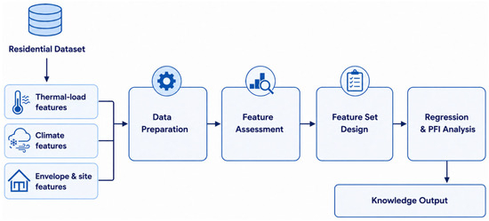
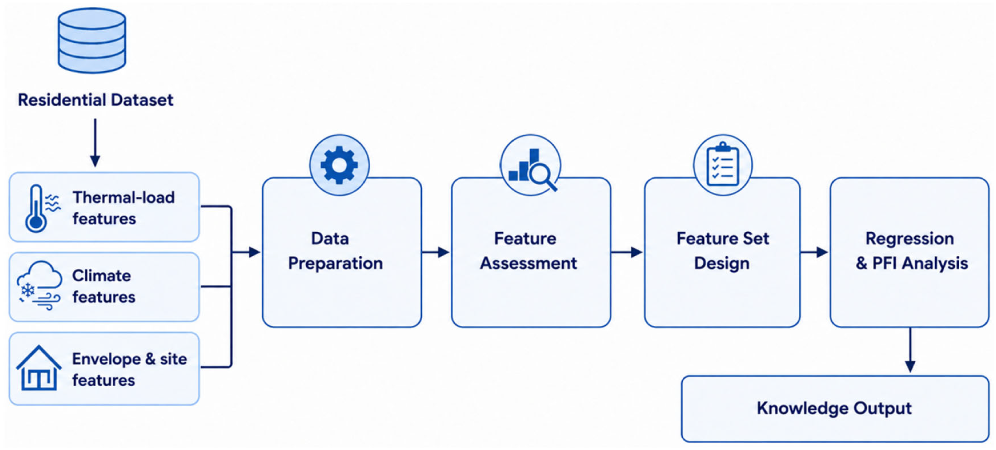
Figure 1 shows the proposed data-driven approach that has been developed and tested. In the following sections, each phase of the proposed approach is explained.

Figure 1. The proposed multi-level data-driven approach for predicting site EUI.

3.1. Data Understanding

The WiDS Datathon 2022 dataset is a publicly available building energy performance dataset designed to analyse site energy use intensity (site EUI) across diverse building types and climates [37]. It contains annual records for approximately 75,757 building instances with 63 features describing physical characteristics (e.g., floor area, year built, facility type), climate descriptors (e.g., temperature summaries, degree days), and energy performance indicators. Each row represents one building over a single calendar year, enabling analysis of annual energy usage patterns. Climate-based variables include monthly temperature statistics that support derivation of cumulative heating and cooling degree days for assessing thermal demand.

Table 2 lists the relevant features including newly derived variables created from the original dataset. Feature selection focused on variables linking climatic forcing to building energy performance while retaining key physical attributes influencing thermal optimisation. Continuous climate indicators such as AAC and AAH reveal climatic variability with median values of about 1285 CDD and 4559 HDD, indicating a heating-dominated climate. Site EUI ranges from 78.1 to 993.4, reflecting substantial performance diversity. Missing values occur in features such as energy star rating (~40%), axwind speed (~47%), and year built (~1%). In contrast, the computed energy features contain no missing data, thus making them suitable for statistical and machine learning analyses. Details of feature derivation are provided in Section 3.2.

Table 2. Sample of Features used from the Original Dataset.

Feature Name	Description	Unit of Measurement	Data Type
Site EUI	Annual site energy use intensity	kBtu/ft2·yr	Continuous
AAC	Annual cumulative cooling degree days	°F-days	Continuous
AAH	Annual cumulative heating degree days	°F-days	Continuous
avg_temp	Mean annual outdoor temperature	°F	Continuous
days_above_90F	Number of extreme hot days (above 90 °F)	Days	Integer
days_below_30F	Number of extremely cold days (below 30 °F)	Days	Integer
floor_area	Gross floor area	ft2	Continuous
year_built	Building construction year	Year	Integer
Elevation	Site elevation	Meters	Continuous
facility_type	Primary building use classification	Category	Categorical
precipitation_inches	Total annual precipitation	inches	Continuous
snowfall_inches	Total annual snowfall	inches	Continuous
max_wind_speed	Maximum wind speed	mph (assumed)	Continuous
CD	Cooling dominance	ratio (0–1)	Continuous
HD	Heating dominance	ratio (0–1)	Continuous

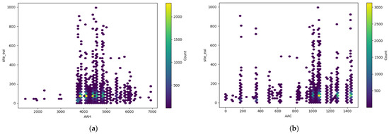
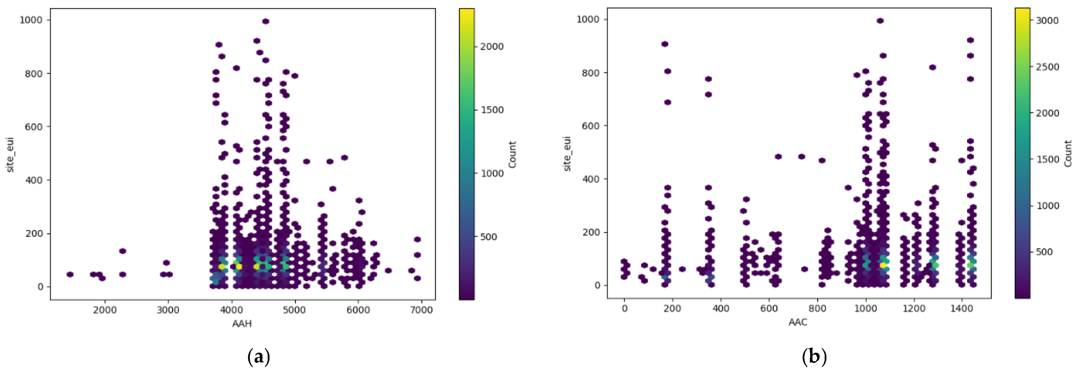
Figure 2a,b illustrates the relationship between some climate features and site EUI while accounting for data density. In the AAC vs. Site EUI case, higher cooling degree days are linked with a wider spread of site EUI values, thus indicating increasing cooling demand and variability in building performance in hot climates. Dense groups at moderate site EUI indicate common cooling operating regimes, while extreme values indicate outliers. On the other hand, the AAH vs. site EUI (see Figure 2a) shows that higher heating degree days correspond to elevated site EUI levels but with diminishing density at extreme HDD values, thereby suggesting threshold effects and diverse heating responses across building types.

Figure 2. The relationship between AAH and site EUI (a) and AAC and site EUI (b).

3.2. Data Filtering and New Features Creation

Since the scope of work is residential buildings, the dataset has been filtered to include only residential buildings; the retained data instances are 43,302 residential building records primarily representing multifamily facilities, and include building characteristics, climate, and energy performance indicators as described earlier. AAC and AAH were computed by aggregating monthly degree indicators weighted by the number of days in each month. This approach preserves the cumulative interpretation of degree days and provides a measure of annual climate-driven thermal demand.

To further contextualise thermal behaviour, dominance ratios were also computed to quantify whether buildings operate under cooling or heating conditions. Climate normalised energy intensity metrics were also computed by relating site energy use intensity to cumulative degree days thereby enabling comparison of energy efficiency independent of climate severity. Additional features such as building age, floor area, and others were retained to capture envelope, scale effects, and thermal stress.

New derived features were formulated to preserve physical meaning, and relevance to building thermal behaviour. Initially, monthly cooling and heating degree indicators were first computed using a base temperature of 65 °F, consistent with standard building energy practice (national weather, n.d.). For each month m, the cooling and heating degree features were calculated as shown in Equations (1) and (2).

$${CDD}_m=max(T_{avg,m}-65.0)$$

(1)

$${HDD}_m=max(65-T_{avg,m}, 0)$$

(2)

where $T_{avg,m}$ and $m$ represent the monthly average outdoor air temperature in degrees Fahrenheit. These indicators quantify the average daily deviation from thermal comfort conditions during each month.

A base temperature of 65 °F was selected because it is the conventional benchmark used in HDD/CDD calculations for building energy analysis and enables consistent comparison across large building datasets [1]. Although actual balance-point temperatures may vary among buildings, the use of a standard base temperature is appropriate for large-scale comparative studies.

To preserve the cumulative nature of degree days, annual values were derived by weighting each monthly indicator by the number of days in the corresponding month and summing across the year as shown in Equations (3) and (4).

$$AAC={\sum }_{m=1}^{12}{CDD}_m\times {days}_m$$

(3)

$$AAH={\sum }_{m=1}^{12}{HDD}_m\times {days}_m$$

(4)

These cumulative features represent the total annual climate-driven thermal demand imposed on a building and form the climate-based drivers used in energy efficiency analysis. Furthermore, to characterise dominant thermal regimes, cooling and heating ratios were derived using Equations (5) and (6). These ratios enable classification of buildings into cooling, heating, or mixed regimes, which is important for thermal load optimisation.

$$CD={\displaystyle \frac{AAC}{AAC+AAH}}$$

(5)

$$HD={\displaystyle \frac{AAH}{AAH+AAC}}$$

(6)

3.3. Feature Selection Methods

For feature selection, CHI, GR, Spearman correlation, distance correlation ($dCor$), and mutual information (MI) have been used to evaluate feature relevance for site EUI. These measures are particularly suitable for energy analysis where predictors are often distributionally heterogeneous. The use of Spearman correlation, $dCor$, and MI is well aligned with the characteristics of the WIDS dataset where both predictors and the class label are continuous. Spearman captures relationships without assuming linearity, while $dCor$ and MI detect general statistical dependence including non-linear interactions, thus making them suitable for relationships that rarely follow linear patterns [38,39]. GR and χ² were applied as complementary methods after discretisation to assess class separability in a categorical setting.

Feature selection analysis was organised into two steps. The first included Spearman, dCor, and MI, which operate on continuous features and capture complex relationships in the dataset. The second used GR and χ², which require discretization, were applied to validate correlation-based results; these methods are widely used in energy efficiency studies [40]. The energy_star_rating variable was excluded as a predictor because it already reflects building energy performance [1].

The χ² statistic measures the degree of dependence between a feature X and a discretised target Y and is defined as follows:

$${\chi }^2(X,Y)={\sum }_{\mathrm{i}}{\sum }_{\mathrm{j}}{\displaystyle \frac{(O_{\mathrm{i}\mathrm{j}}-E_{\mathrm{i}\mathrm{j}}{)}^2}{E_{\mathrm{i}\mathrm{j}}}}$$

(7)

where O_ij and E_ij denote the observed and expected joint frequencies of feature category i and target class j, respectively.

GR evaluates the information provided by a feature while penalising high intrinsic entropy. It is defined as follows:

$$GR={\displaystyle \frac{IG}{Split Information}}$$

(8)

$$IG(S,A)=H(S)-{\sum }_v{\displaystyle \frac{\left|Sv\right|}{\left|S\right|}}·H(Sv)$$

(9a)

$$Split Information\left(S,A\right)=-{\sum }_v{\displaystyle \frac{\left|Sv\right|}{\left|S\right|}}·{log}_2({\displaystyle \frac{\left|Sv\right|}{\left|S\right|}})$$

(9b)

IG (S, A) is the information gain of attribute A relative to dataset S; H(S) is the entropy of the dataset S; S_v is the subset of S where attribute A takes value v; |S_v| is the number of instances in subset S_v; |S| is the total number of instances in dataset S; H(S_v) is the entropy of subset S_v.

Initially, and for each feature, the χ² and GR scores were rescaled using the min–max normalisation method to map all values to the [0, 1] range, thus ensuring comparability across methods per Equation (12).

$$x\text{\_}norm={\displaystyle \frac{x-min\left(x\right)}{max\left(x\right)-min\left(x\right)}}$$

(10)

In addition to χ² and GR, correlation and information theory methods were used to assess robustness across linear, monotonic, and non-linear dependency structures. Spearman’s rank correlation coefficient ρ_s measures monotonic association and is defined as follows:

$${\rho }_{\mathrm{s}}=1-({\displaystyle \frac{6\sum d{ᵢ}^2}{n\left(n^2-1\right)}})$$

(11)

where d_i is the rank difference between paired observations, while MI measures the total shared information between variables:

$$I(X;Y)={\mathit{\sum }}_{\mathrm{x}}{\mathit{\sum }}_{\mathsf{\gamma }}p(x,y){log}_2({\displaystyle \frac{p\left(x,y\right)}{p\left(x\right)p\left(y\right)}})$$

(12)

To further capture non-linear dependence without parametric assumptions, dCor, was used:

$$dCor(X,Y)={\displaystyle \frac{dCov(X,Y)}{\sqrt{dVar\left(X\right)dVar\left(Y\right)}}}$$

(13)

Finally, a global score was then computed as the arithmetic mean of the normalised values for each feature selection method used. The discretised site EUI classes were used exclusively for the CHI and GR feature selection and were not used in the subsequent regression modelling or PFI analyses.

3.4. Models Building and Validation

For the regression-based modelling, linear regression has been used to model site EUI as a linear combination of explanatory variables by minimising the sum of squared residuals. Given predictors $x_1,\dots ,x_p,$ the model is as follows:

$$\hat{\mathrm{y}}={\beta }_0+{\beta }_{1}x$$

(14)

where β₀ = intercept, β₁ = slope, x = independent variable and $\hat{\mathrm{y}}$ = Predicted value.

However, building energy predictors such as AAH, AAC, and dominance ratios are often highly correlated, which can destabilise OLS estimates. To address this, regularised regression methods are employed.

Ridge regression adds an L2 penalty that shrinks coefficients while keeping all variables:

$$min{\sum }_{i=1}^n{(y_i-{\sum }_{j=1}^p{{\beta }_{j}x}_{ij})}^2+\lambda {\sum }_{j=1}^p{{\beta }_j}^2$$

(15)

where λ ≥ 0 controls the degree of shrinkage. Ridge is effective when predictors are collinear as it distributes weights among related features.

Lasso regression introduces an L1 penalty to encourage sparsity:

$$min{\sum }_{i=1}^n{(y_i-{\sum }_{j=1}^p{{\beta }_{j}x}_{ij})}^2+\lambda {\sum }_{j=1}^p\left|{\beta }_j\right|$$

(16)

Unlike ridge, lasso can force some βj = 0, identifying the most influential climate or thermal predictors.

For the model validation, RMSE and R² were used. RMSE measures the average magnitude of prediction errors:

$$RMSE=\sqrt{{\displaystyle \frac{1}{n}}{\sum }_{i=1}^n{{(y}_i-{\hat{y}}_i)}^2}$$

(17)

where:

• n = number of observations,
• $y_i$ = actual value,
• ${\hat{y}}_i$ = predicted value.

R² measures the proportion of variance explained by the model.

4. Results Analysis

4.1. Experimental Settings and Testing Protocol

For the Spearman correlation, dCor, and MI experiments, no data discretisation was performed because these methods are designed to evaluate relationships between continuous predictor variables and the continuous site EUI target label. Prior to analysis, missing values in max_wind_speed were imputed using the median value of the feature to minimise the influence of outliers, while records containing missing values in year_built were excluded from the corresponding calculations. Spearman correlation coefficients were computed using the spearmanr() function from the SciPy library. MI was estimated using the mutual_info_regression() function from scikit-learn with the default k-nearest neighbour estimator to enable the detection of non-linear dependencies between predictors and site EUI. dCor was implemented using NumPy-based calculations following the formulation of [18] to allow the identification of both linear and non-linear associations.

For the IG, GR, and CHI experiments, discretisation was required because these methods operate on categorical data. Continuous predictor variables were discretised using the KBinsDiscretizer function from scikit-learn with a fixed-width binning strategy, while site EUI was transformed into discrete categories using equal-width intervals. IG was calculated as the reduction in entropy achieved by partitioning the target variable according to each predictor. GR was subsequently derived by dividing IG by the intrinsic information (split information) of the corresponding feature to reduce the bias of IG towards variables with many distinct values. CHI scores were computed using the chi2() function from scikit-learn, which evaluates the statistical dependence between discretised predictor variables and the discretised site EUI classes.

Since the feature selection methods generate scores on different numerical scales, direct comparison is not meaningful. Therefore, the scores produced by each method were normalised independently using Min-Max scaling through scikit-learn’s MinMaxScaler, transforming all scores to the range [0, 1]. A global relevance score was then calculated for each feature as the arithmetic mean of the normalised scores obtained from Spearman correlation, DI, MI, IG, GR, and CHI analyses. This aggregation strategy provides a consensus ranking that balances the strengths of individual feature selection methods and reduces the influence of any single metric.

The testing protocol was designed to evaluate whether different feature groups provide incremental predictive value for site EUI estimation. First, the dataset was pre-processed by excluding potentially biasing or highly incomplete variables including energy_star_rating and year_built, while missing values in continuous variables such as max_wind_speed were handled using median imputation. The selected features were then organised into five feature sets (A–E) derived from the earlier feature relevance analysis, global ranking scores, and PFI results. These sets were designed to compare primary thermal indicators, combined heating and cooling indicators, extended climate-site variables, PFI-selected variables, and the full available feature set. This structure allowed the experiments to test not only overall prediction accuracy, but also the marginal contribution of each feature group.

For thermal model development, regression algorithms were implemented in Python 3.12: linear regression, ridge regression, and lasso regression. Each model was evaluated across distinct feature sets using 10-fold cross-validation to reduce dependence on a single train-test split and to provide more robust performance estimates. Model performance was assessed using RMSE and R², with results reported as mean values across folds. RMSE was used to measure prediction error magnitude, while R² was used to evaluate the proportion of site EUI variance explained by each model-feature-set combination. The results were then compared across feature sets and algorithms to determine whether compact thermal and climate feature groups could perform comparably to, or better than, larger feature sets containing additional envelope and site-context variables.

4.2. Feature Selection Results

Table 3 shows feature relevance to site EUI using Spearman correlation, dCor, and MI methods, in addition to a global score column. Results show that the most influential features are snowfall_inches (0.977), AAC (0.854), CH (0.848), HD (0.835), days_below_30F (0.815), and AAH (0.811). These features quantify cumulative heating and cooling stress and extreme cold exposure, which translate into higher HVAC use. Prior research studies show that degree day-based features and dominance indices can explain a share of EUI variance across diverse climates; thus, they often outperform other descriptors in data-driven models [38,39,41].

Table 3. Features scores and ranking using Spearman, dCor, and MI methods.

Feature	Spearman	Spearman Rank	Spearman_ Normalised Score	dCor	dCor Rank	dCor_Normalised Score	MI	MI Rank	MI_Normalised Score	Global Score	Global Rank
snowfall_inches	0.264	1	1	0.31	4	0.93	0.42	2	1	0.977	1
AAC	0.156	6	0.565	0.33	2	0.998	0.42	1	0.999	0.854	2
CD	0.16	4	0.582	0.33	1	1	0.41	3	0.961	0.848	3
HD	0.16	4	0.582	0.32	3	0.965	0.4	8	0.958	0.835	4
days_below_30F	0.183	3	0.676	0.27	5	0.776	0.42	6	0.956	0.815	5
AAH	0.217	2	0.813	0.23	6	0.622	0.42	4	0.997	0.811	6
precipitation_inches	0.089	8	0.294	0.12	10	0.194	0.42	7	0.999	0.496	7
days_above_90F	0.075	9	0.237	0.18	8	0.431	0.33	9	0.775	0.481	8
avg_temp	0.016	13	0	0.14	9	0.26	0.42	5	0.996	0.419	9
year_built	0.11	7	0.38	0.18	7	0.437	0.1	12	0.209	0.342	10
Elevation	0.033	12	0.068	0.08	12	0.033	0.19	10	0.433	0.178	11
floor_area	0.034	11	0.072	0.1	11	0.104	0.12	11	0.248	0.141	12
max_wind_speed	0.055	10	0.155	0.07	13	0	0.02	13	0	0.052	13

Feature grouping is justified using a global score drop-off equation:

Drop_{i → j} = (G_i − G_j)/G_i

(18)

For example, the drop from AAC (0.854) to precipitation_inches (0.496) equals 41.9%, and from AAH (0.811) to precipitation_inches (0.496) equals 38.8% indicating closure of a high impact feature set. Based on this behaviour of the feature ranking, at least when using these feature selection methods, some feature groups can be suggested as follows:

• Group 1—Primary climate and thermal feature set (top 6)
• Group 2—Secondary climate and temporal proxies (ranks 7–10)
• Group 3—Envelope and site context, such as elevation, floor area, and wind speed

Across methods, MI and Spearman consistently rank Group 1 features highest while dCor emphasises non-linear sensitivity in cooling related features, thus supporting climate, then thermal features.

The CHI and GR results (Table 4) extend the patterns identified by the previous results reported by Spearman, dCor, and MI methods, demonstrating consistency while revealing complementary sensitivities. For example, climate, and thermal features remain dominant with HD, snowfall_inches, AAH, AAC, CD, and days_below_30F occupying the highest global ranks. Notably, CHI emphasises features associated with overall separation power (e.g., HD with the highest CHI score), whereas GR highlights features that provide informative splits, such as days_above_90F, which ranks lower in correlation-based methods but rises under GR results. This divergence reflects that correlation and MI methods favour global dependency strength while GR prefers features that efficiently partition the response space particularly under non-uniform distributions.

Table 4. Feature ranking of the considered filter methods scores after data normalisation.

Feature Name	CHI Score	CHI Normalised Feature Score	CHI Normalised Feature Rank	GR Score	GR Normalised Feature Score	GR Normalised Feature Rank	Global Score	Global Rank
HD	3595.593	1.000	1	0.061	0.565	6	0.782255	1
snowfall_inches	2966.939	0.807	2	0.070	0.659	3	0.732673	2
AAH	2383.784	0.627	4	0.069	0.647	4	0.63721	3
AAC	2379.960	0.626	5	0.068	0.645	5	0.635436	4
CD	2431.860	0.642	3	0.061	0.565	6	0.603386	5
days_below_30F	989.896	0.199	7	0.099	0.975	2	0.587192	6
days_above_90F	722.228	0.117	10	0.101	1.000	1	0.558355	7
year_built	1937.801	0.490	6	0.024	0.164	11	0.32702	8
floor_area	791.242	0.138	9	0.047	0.417	7	0.277355	9
avg_temp	855.754	0.158	8	0.034	0.273	8	0.215225	10
precipitation_inches	408.312	0.020	11	0.034	0.272	9	0.146189	11
Elevation	381.033	0.012	12	0.025	0.177	10	0.094238	12
max_wind_speed	342.572	0.000	13	0.008	0.000	12	0	13

HVAC system sizing, operational efficiency, and control schemes are dictated by sustained cold or hot periods rather than annual averages [1]. Recent research studies confirm that climate intensity and persistence metrics outperform static building features in explaining regional variations in building energy use [5]. From a feature selection results perspective, the results indicate that climate and thermal features rank higher than static building descriptors such as floor area, or elevation, at least using the data and feature selection methods considered. Thermal loads are governed by external conditions rather than by average climate-based conditions or individual building features when analysed at a national scale [40].

Quantitatively, CHI and GR global scores drop from approximately 0.56–0.78 for the top ranked thermal features to below 0.33 for year_built and floor_area, mirroring the separation previously observed in MI, dCor, and Spearman methods’ results. Envelope and site features remain low ranked in both results analyses.

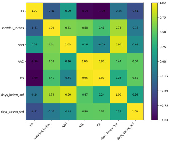
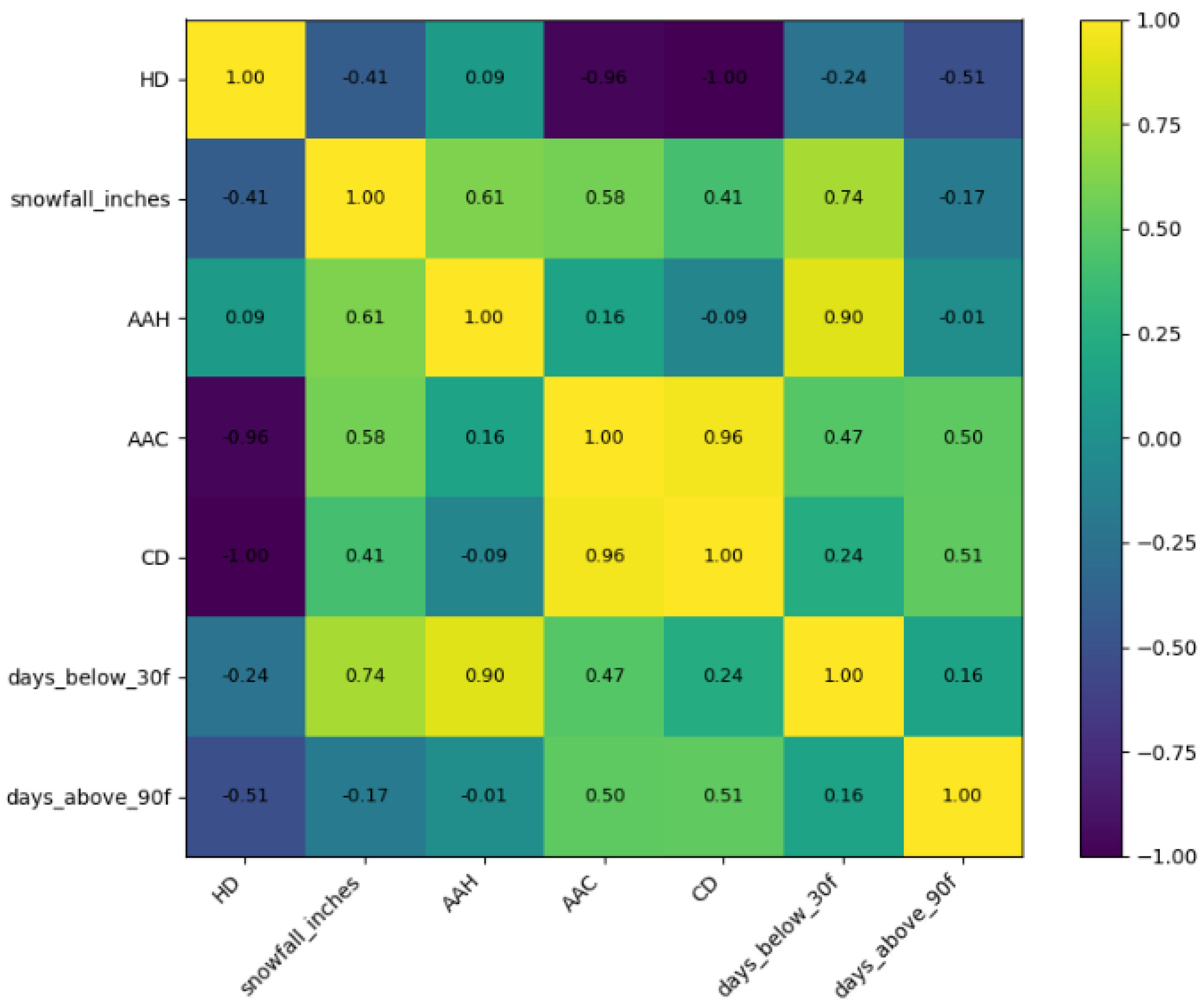
Figure 3 illustrates the feature-feature correlations among the top ranked thermal and climate features using Spearman correlation method to highlight groupings between heating and cooling features. This enables the identification of the possible redundant features besides different features in terms of similarity, at least using Spearman correlation measure. Strong positive monotonic relationships are observed among heating features; for instance, the correlation between AAH and days_below_30F (ρ = 0.90), and the correlation between snowfall_inches and days_below_30F (ρ = 0.69). These relationships indicate that cumulative heating demand, frequency of extreme cold days, and snowfall jointly represent cold climate severity rather than independent effects. The moderate association between snowfall_inches and AAH (ρ = 0.63) further echoes this interpretation and, thus, suggests partial redundancy within the heating feature subset. Cooling features form a distinct and highly cohesive cluster. AAC and CH exhibit a positive monotonic relationship, thus confirming that dominance metrics are largely derived from cumulative cooling demand. In contrast, HD shows a perfectly negative relationship with CD and a strong negative correlation with AAC, reflecting mutually exclusive climatic control regimes. Cross-group correlations remain weak, such as AAH versus AAC (ρ = −0.19), which indicates that heating and cooling loads are driven by different climatic processes rather than co-varying uniformly. Transitional indicators such as days_above_90F align moderately with cooling variables (ρ = 0.65 with AAC; ρ = 0.61 with CH) while remaining weakly or negatively related to heating indicators, which support the separation of thermal regimes observed in feature selection results.

Figure 3. Spearman correlation for thermal load features vs. site EUI.

4.3. PFI Analyses

PFI analyses have been conducted on the dataset with RMSE as the evaluation metric to reveal feature interactions besides their contribution to the models’ performance. Two base learners are used: LASSO regression and linear regression from the scikit-learn Python library. Missing values are handled by excluding year_built as a feature, and median imputation is applied to max_wind_speed and other numeric features. PFI is computed with sklearn repeating permutations 10 times for stability. RMSE was selected as a performance metric, which measures how far a model’s predictions are from the actual values to ensure fair evaluation of both common and rare energy-use settings.

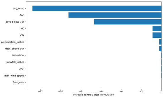
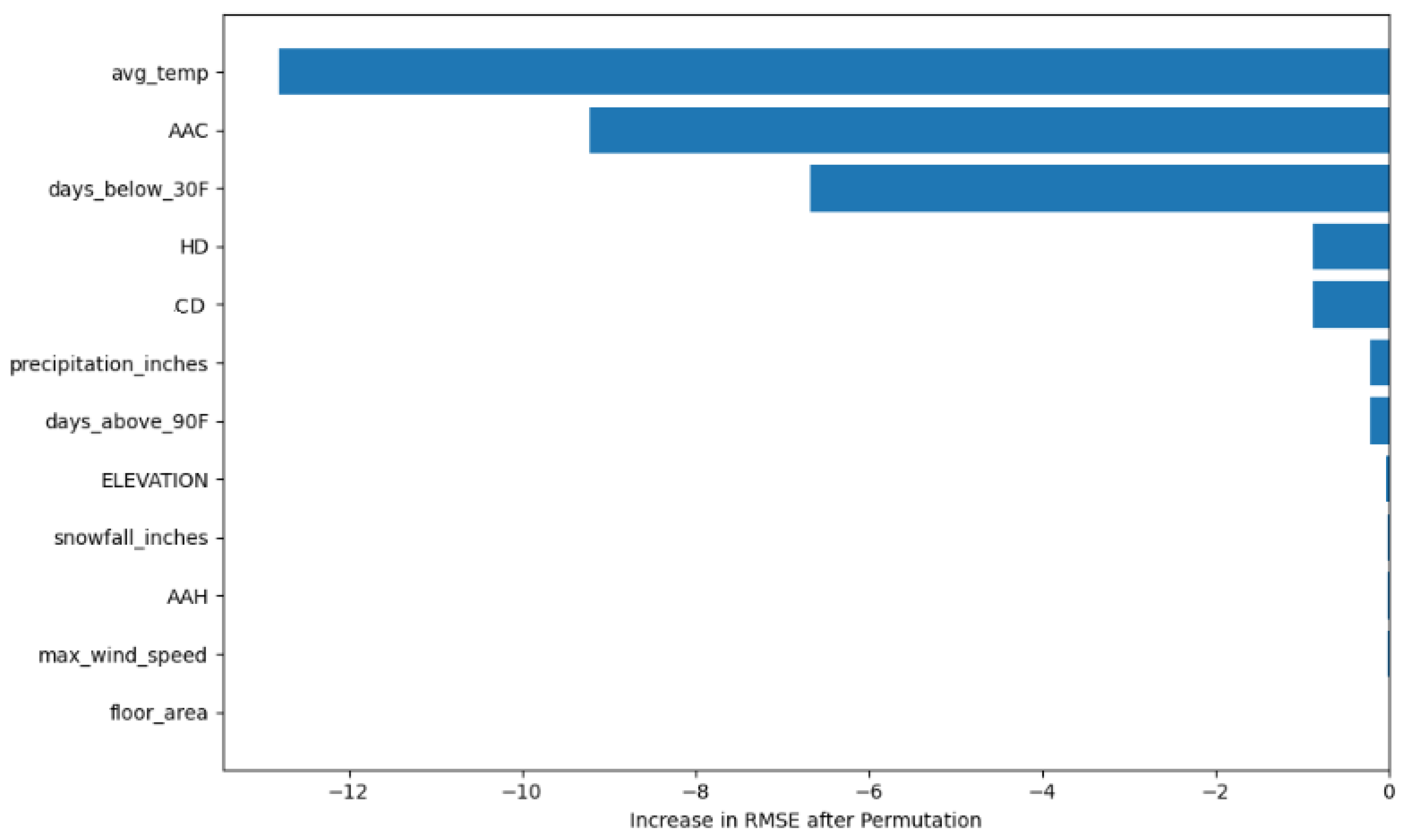
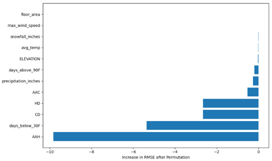
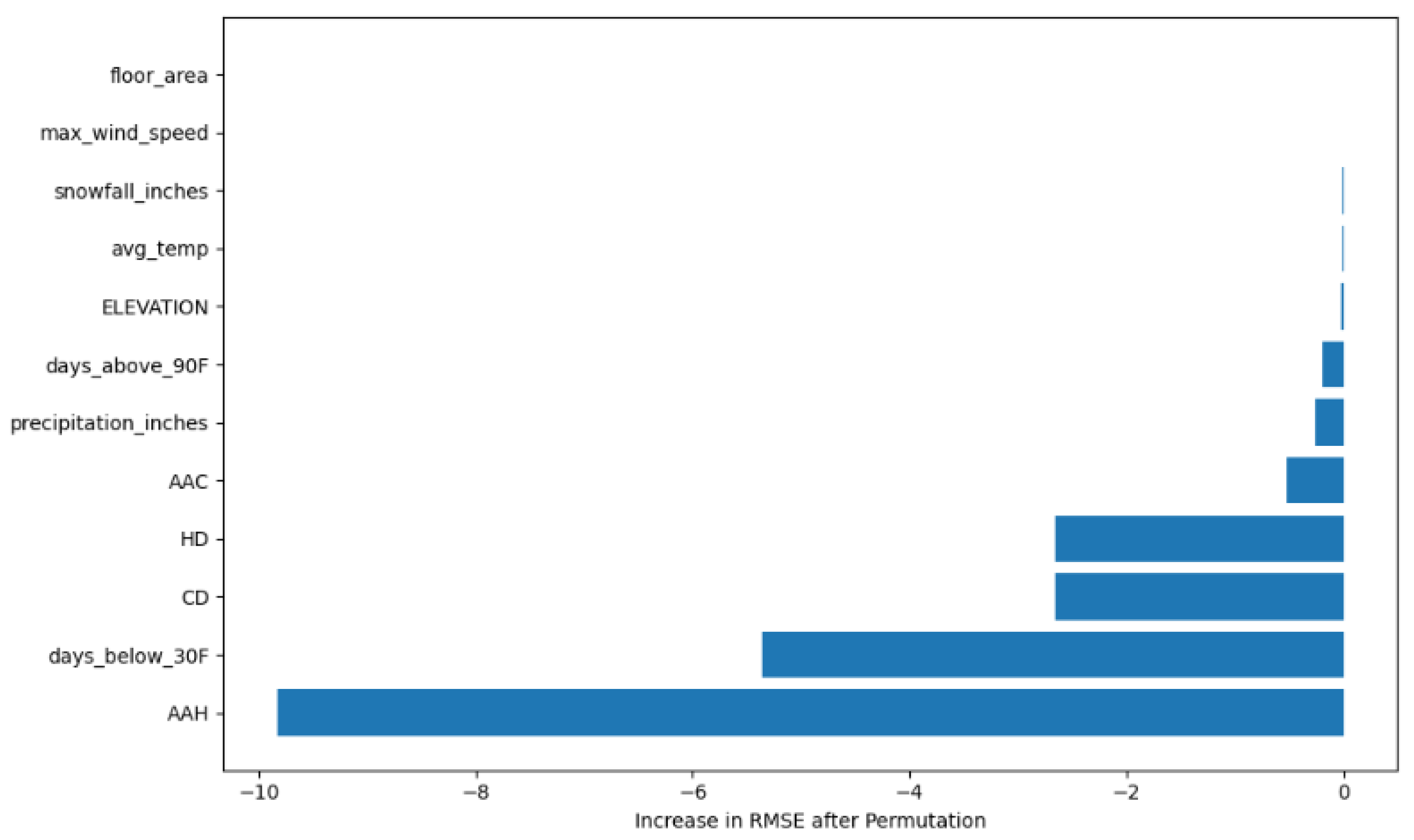
The PFI analyses from both ridge regression and linear regression algorithms (Figure 4 and Figure 5) consistently show that climate related features are the dominant drivers of site EUI. In the ridge model, average temperature, AAC, and days below 30 °F produce the largest increases in RMSE when permuted, thus indicating that the model relies heavily on thermal demand indicators. Similarly, the linear regression PFI analyses highlight AAH, days below 30 °F, and cooling/HD indices as major contributors. The exact ranking differs slightly between models due to how each handles multicollinearity and coefficient shrinkage. The results show some variations such as in the PFI’s rank of certain features like average temperature (avg_temp). This can be due to the fact that ridge algorithm (with regularisation) distributes feature importance across correlated climate features, while linear regression (without regularisation) shifts weight towards more specific temperature-related features like AAH. This reflects each algorithm’s behaviour under multicollinearity: ridge stabilises shared predictors, whereas linear regression lets correlated features compete, thus causing importance to move between related features of the same type.

Figure 4. Features contributions in terms of RMSE using PFI ridge regression.

Figure 5. Features contributions in terms of RMSE using PFI linear regression.

Secondary features such as precipitation, snowfall, elevation, and wind speed show little impact in both models, thereby suggesting they play a limited role in predicting overall EUI within this dataset (residential buildings) and using the algorithms considered. Building size (floor area) also remains a weak predictor compared to climate-driven features. From an energy optimisation perspective, these results echo that approaches targeting heating and cooling loads such as insulation upgrades, building design, and smart temperature controls can offer good potential for reducing site EUI, at least using the methods used and data examples considered.

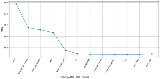
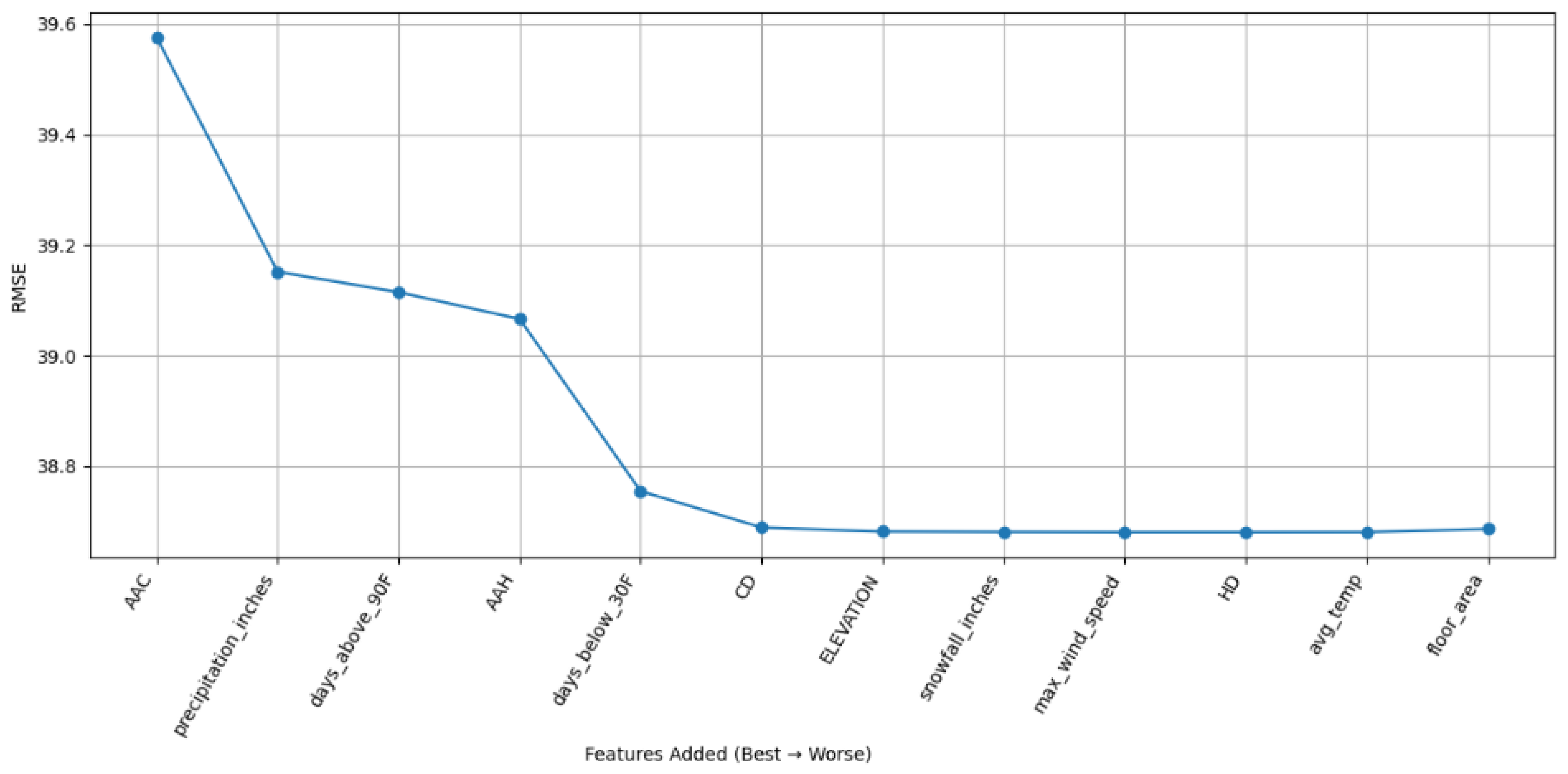
To further verify feature importance in terms of predictive model performance, a linear regression algorithm was applied to the dataset after excluding year_built by considering adding features one by one and recording the RMSE measurement on the model derived as shown in Figure 6. The results of that figure illustrate that the largest reductions in error occur with early added climate features such as AAC, precipitation_inches, days_above_90F, and AAH, confirming that heating and cooling demand indicators carry the strongest predictive signal. A further noticeable drop appears when days_below_30F and HD are introduced after which the curve begins to flatten. Once elevation and snowfall_inches are added, RMSE stabilises, thus indicating diminishing returns from additional features. Subsequent features like wind speed, CD, average temperature, and floor area provide minimal improvement and may add noise rather than useful signal. Therefore, feature addition should stop after snowfall_inches, with the recommended set being: AAC, precipitation_inches, days_above_90F, AAH, days_below_30F, HD, elevation, and snowfall_inches.

Figure 6. RMSE vs. feature addition order (Best to Worst) using linear regression algorithm.

5. Regression Experimental Results

5.1. Experiments Settings

The experiments were conducted using Python (scikit-learn) with a 10-fold cross-validation. Energy_star_rating was excluded to avoid model overfitting. Year_built was also ignored due to excessive missing values. No data normalisation or discretisation was applied to either independent features or the class label, preserving the original measurement scales. Missing values in the remaining continuous features (including max_wind_speed) were handled using median imputation.

Different linear regression algorithms were employed to evaluate thermal, climate and envelope-related features of the considered dataset (linear regression, ridge, and lasso). The default hyperparameters were used for the considered algorithms. Model testing was assessed using 10-fold cross-validation implemented using Kfold and cross_validate. Evaluation metrics included RMSE and R², computed using mean_squared_error, r2_score, and custom scorers created with make_scorer. Final results were reported as the mean and standard deviation across folds.

Multiple experiments have been performed on the feature sets shown in Table 5 based on the earlier feature assessment and PFI analyses.

Table 5. Selected distinct feature sets with description.

Feature Set Label	# of Features	List of Features
A	5	HD, AAH, AAC, snowfall_inches, days_above_90F
B	6	AAC, AAH, days_below_30F, HD, CD, snowfall_inches
C	8	snowfall_inches, AAC, AAH, days_above_90F, days_below_30F, max_wind_speed, floor_area, Elevation
D	8	AAC, precipitation_inches, days_above_90F, AAH, days_below_30F, HD, Elevation, snowfall_inches
E	12	floor_area, Elevation, precipitation_inches, snowfall_inches, avg_temp, days_below_30F, days_above_90F, max_wind_speed, AAC, AAH, CD, HD

5.2. Model Analysis

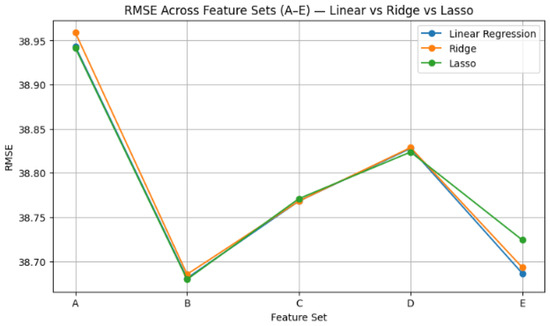
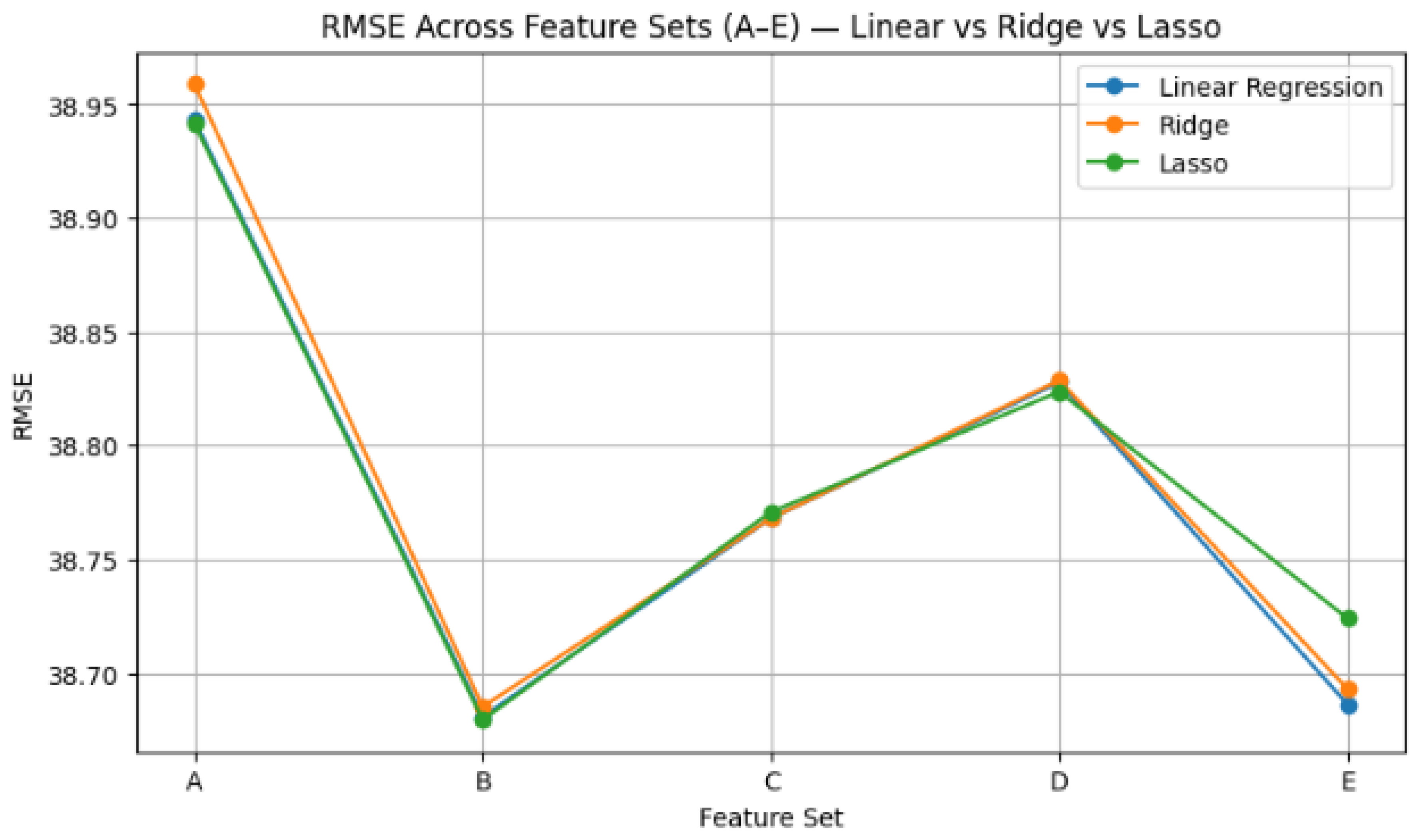
Figure 7 shows the RMSE differences of the derived models across the feature sets. Models derived from feature set B consistently deliver the lowest RMSE for all three algorithms (linear, ridge, and lasso), indicating that, when this data subset is processed by regression algorithms, the models developed provide the most accurate predictions of site EUI, at least when using the dataset/features considered. This suggests that the combination of cooling and HD, degree days (CDD/HDD), extreme cold days, and snowfall captures the most relevant climatic drivers of building energy demand. Further, feature set E (the full set without year built) performs second best for linear and ridge but slightly worse for lasso, implying that adding more features such as floor area and wind speed provides marginal gains but also introduces some noise or redundancy at least when using the considered dataset and the algorithms used. Feature sets C and D show moderate RMSE, meaning that they contain useful weather severity indicators but may lack balanced representation of both heating and CD.

Figure 7. RMSE results from regression algorithms on distinct sets of features.

The high ranking of thermal and climate indicators observed in this study is consistent with the physical operation of residential buildings, where heating and cooling demands account for a proportion of annual energy consumption. Features such as accumulated heating and cooling degree days, heating and cooling dominance ratios, and extreme temperature indicators capture climate-driven thermal demand and therefore have a direct influence on site EUI. Similar observations have been reported in previous studies, which identified climate variables as drivers of building energy performance and energy consumption patterns across residential building stocks [5,9,38]. The results are also aligned with [12], who demonstrated that thermal load characteristics provide predictive indicators in residential building energy models despite the fact that the dataset used by the authors is simulated and small. From a practical perspective, the findings suggest that indicators related to thermal and climate can be considered potential baseline variables for data analyses focused on energy optimisation studies.

However, despite the consistent ranking of thermal and climate features, the relatively low R² values indicate that these variables alone cannot fully explain Site EUI variability. Building energy consumption is also influenced by factors such as HVAC system efficiency, insulation quality, building configuration, occupancy behaviour, and building material, among others, many of which are not represented in the WiDS dataset. Consequently, the findings should be interpreted primarily as evidence of the relative importance of feature groups of buildings in the context of thermal load rather than as a basis for energy planning decisions. These missing building-specific characteristics likely contribute to the modest explanatory power observed across all evaluated models.

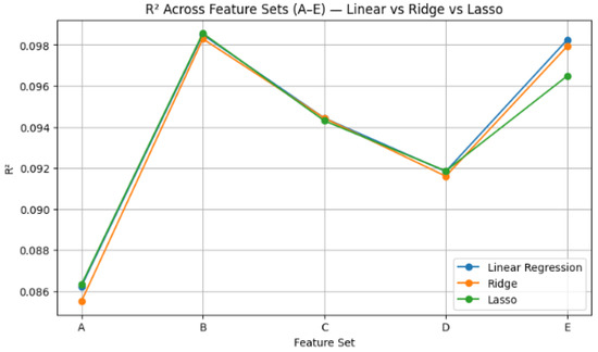
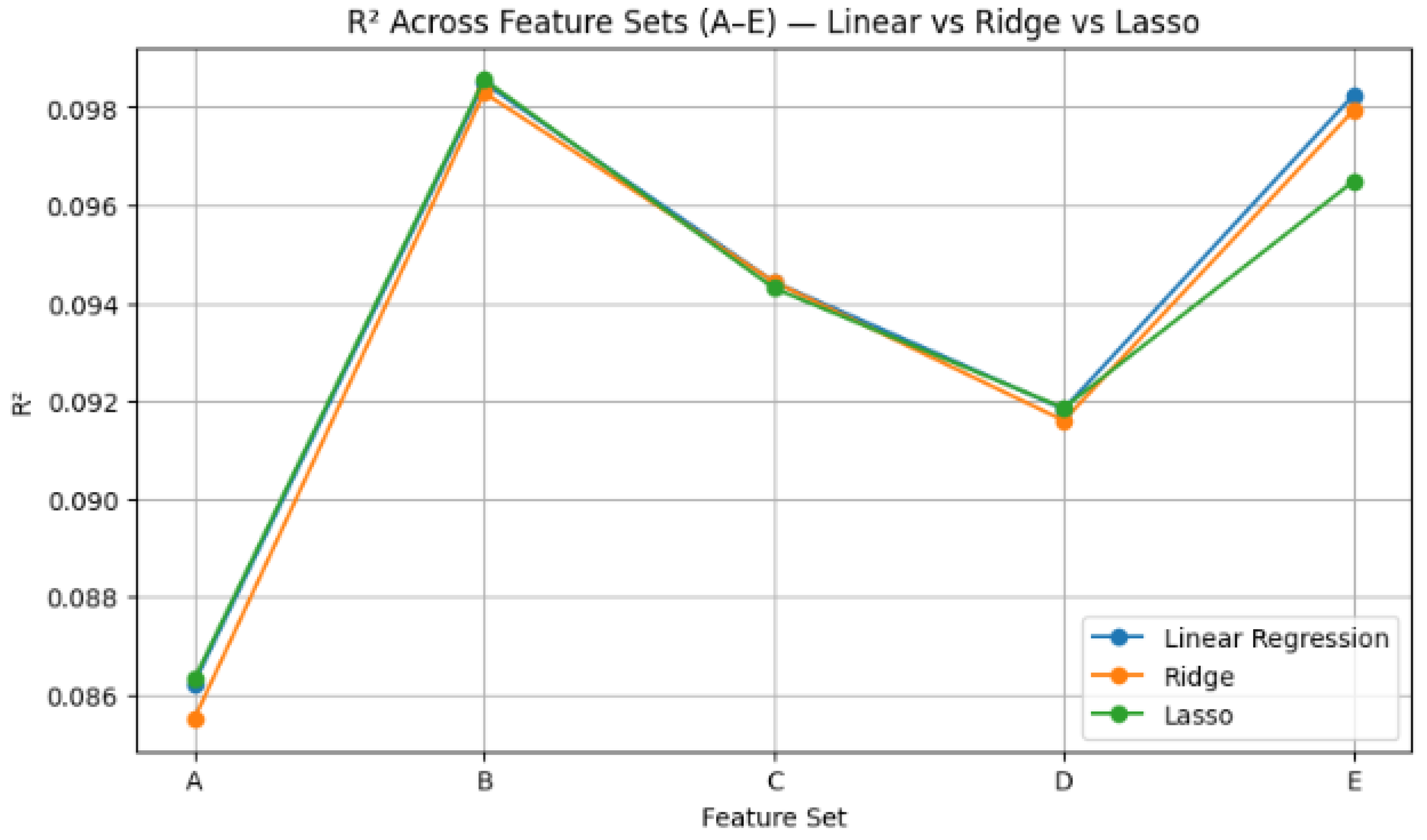
Figure 8 shows R² performance of the regression-based algorithms on the distinct feature sets. The results mirror the RMSE trends and echo the relative effectiveness of the feature subsets. Feature set B, when processed by the regression algorithms, derived models that achieve the highest R² values across all three models, thus explaining the largest proportion of variance in site EUI. This aligns with its lowest RMSE, confirming that the features in set B, especially cooling/HD and degree-day metrics, capture the core climatic drivers of building energy demand and thermal load.

Figure 8. R² results from regression algorithms on distinct sets of features.

Figure 7 and Figure 8 compare the performance of three regression models (linear regression, ridge, and lasso) across different feature sets (A–E), using the R² score as the evaluation metric. Overall, the three models show very similar trends, thus indicating that regularisation does not substantially change predictive performance in this case. Feature set B shows slightly higher R² compared to the results shown in Set A for all models, suggesting that it contains more informative features. Feature sets C and D yield intermediate performance while set E again leads to a relatively high value, though slightly below those of set B.

The results in Figure 7 and Figure 8 indicate that performance differences among linear, ridge, and lasso regression are very small across all feature subsets, at least when using the considered dataset: R² remains low and closely clustered for every model-subset combination. This consistency suggests that model choice has limited influence compared with the inherent information content of the available features in the dataset. It also shows that none of the feature subsets provides strong explanatory power for site EUI, thereby making it difficult to distinguish which subset is truly superior, despite the higher rank for thermal and climate-based features. The modest R² values imply that large portions of energy use variability remain unexplained when processing the WiDS dataset. Therefore, additional building-specific material and system-efficiency features may be needed to improve thermal load prediction and support more reliable energy optimisation approaches.

These findings are also related to the questions raised in Section 1. The selected feature selection algorithms, regression methods, and PFI algorithm have ranked the same features (AAH, AAC, HD, CD, snowfall, and extreme temperatures) as the most important factors explaining the variation in site EUI. On the other hand, the inclusion of additional evaluated categories of the envelope and site-specific features led only to marginal improvements in terms of prediction accuracy for the analysed feature sets. The low values of R² also mean that the evaluated climate and envelope characteristics do not sufficiently explain the site EUI variation.

6. Conclusions

This research investigated the degree of influence of different types of features on site EUI using the building energy dataset from the WiDS Datathon 2022. To address this problem, a data-driven approach based on feature evaluation, PFI, and regression analysis was proposed to assess the contribution of different groups of features to site EUI prediction.

The proposed approach evaluated feature importance using CHI and GR analyses, correlation analysis, and regression experiments across different feature subsets. The feature ranking results showed that the six highest ranked thermal features (HD, snowfall_inches, AAH, AAC, CD, and days_below_30F) achieved global scores ranging from 0.56 to 0.78, whereas building and site descriptors such as floor_area scored below 0.33. Correlation analysis further demonstrated clustering within thermal regimes, with AAH and days_below_30F exhibiting a strong relationship. Consistent with these findings, regression experiments showed that the feature subset dominated by thermal indicators (Set B) achieved the lowest RMSE (approximately 38.68) and the highest R². In addition, incremental feature analysis showed that RMSE improvements became marginal after the first six climate features, indicating diminishing predictive returns beyond the core thermal indicators.

These findings indicate that climate and thermal features provide greater predictive capability for site EUI than the other investigated feature groups. The proposed approach facilitates the analysis of site EUI by evaluating dissimilar groups of features using multiple evaluation parameters, thereby helping identify informative predictors and quantify the contribution of each feature group. However, the relatively low R² values and modest RMSE improvements indicate that the current dataset explains only a limited proportion of site EUI variability. Therefore, the results should be interpreted primarily as evidence of relative feature importance rather than as a basis for direct HVAC design or energy management decisions.

The limited predictive performance is likely attributed to the characteristics of the available dataset. Most predictors represent climate severity indicators, including degree days, extreme temperature days, snowfall, and wind, which describe environmental demand rather than building-specific performance. Important explanatory variables, including insulation characteristics, glazing type, HVAC system efficiency, occupancy density, operating schedules, retrofit history, building layouts, and other structural characteristics, are absent. Furthermore, the annual aggregation of weather variables masks seasonal and daily load variations, while correlations among some predictors (e.g., HD and HDD) may introduce redundancy without providing additional information. Since site EUI is influenced by both climate conditions and building operational behaviour, the absence of detailed building characteristics limits the predictive capability of the regression models.

Future work will incorporate additional building material, structural, envelope, and occupancy-related features to further evaluate predictive performance. Higher temporal resolution climate variables will also be considered to better capture seasonal and daily thermal demand. In addition, future studies will investigate rule-based induction models and hybrid physics-data approaches to improve model performance and capture nonlinear feature interactions. Finally, the generalisability of the proposed approach should be evaluated across unseen climate zones and residential building types using richer datasets, such as ResStock, to determine whether the relative importance of thermal, climate, and envelope feature groups remains consistent under different climatic conditions and building archetypes.

References

- American Society of Heating, Refrigerating and Air-Conditioning Engineers (ASHRAE). ASHRAE Handbook—Fundamentals, SI ed.; American Society of Heating, Refrigerating and Air-Conditioning Engineers (ASHRAE): Atlanta, GA, USA, 2021. [Google Scholar]
- Santamouris, M. Advances in Building Energy Research; Earthscan: London, UK, 2012; Volume 3. [Google Scholar]
- Aloshan, M.A.; Aldali, K.M. Courtyard design for energy efficiency and thermal comfort: Machine learning insights across hot and warm climates. Sci. Rep. 2025, 15, 43660. [Google Scholar] [CrossRef] [Scilit] [PubMed]
- Marzouk, O.A. Summary of the 2023 report of TCEP by IEA and proposed process for computing a single aggregate rating. E3S Web Conf. 2025, 601, 00048. [Google Scholar] [CrossRef] [Scilit]
- Guo, Y.; Li, X.; Zhang, Y.; Wang, S. Climatic impacts on electricity consumption of urban residential buildings. Energy Build. 2025, 293, 113206. [Google Scholar]
- Kusumastuti, D.; Setyowati, E.; Sari, S.; Dwiyanto, A. Analysis of Energy Use Intensity (EUI) Factors in Government Office Buildings in Tropical Climate: A Case Study in the Ministerial Office Building and the Directorate General of Water Resources Building of The Ministry of Public Works. TEKNIK 2025, 46, 209–217. [Google Scholar] [CrossRef] [Scilit]
- Abdul-Zahra, A.S.; Al-Haddad, L.A.; Abdulsahib, I.A.; Kraiem, H.; Flah, A. Sustainable thermal load prediction in residential buildings using machine learning: A case study analysis. Results Eng. 2025, 27, 106872. [Google Scholar] [CrossRef] [Scilit]
- Nguyen, N.M.; Cao, M.T. Energy use intensity analysis using green BIM-integrated interpretable machine learning. J. Build. Eng. 2025, 108, 112760. [Google Scholar] [CrossRef] [Scilit]
- Sailor, D.J. Relating residential and commercial sector electricity loads to climate. Energy 2001, 26, 645–657. [Google Scholar] [CrossRef] [Scilit]
- Zhao, H.-X.; Magoulès, F. A review on the prediction of building energy consumption. Renew. Sustain. Energy Rev. 2012, 16, 3586–3592. [Google Scholar] [CrossRef] [Scilit]
- Kömürcü, D.; Edis, E. Machine learning modeling for building energy performance prediction based on simulation data: A systematic review of the processes, performances, and correlation of process-related variables. Buildings 2025, 15, 1301. [Google Scholar] [CrossRef] [Scilit]
- AbdelJaber, F.; Dirks, K.N. Thermal load prediction in residential buildings using interpretable classification. Buildings 2024, 14, 1989. [Google Scholar] [CrossRef] [Scilit]
- Mahmood, T.; Asif, M. Prediction of energy efficiency for residential buildings using supervised machine learning algorithms. Energies 2024, 17, 4965. [Google Scholar] [CrossRef] [Scilit]
- Cui, X.; Lee, M.; Koo, C.; Hong, T. Energy consumption prediction and household feature analysis for different residential building types using machine learning and SHAP: Toward energy-efficient buildings. Energy Build. 2024, 309, 113997. [Google Scholar] [CrossRef] [Scilit]
- Alrobaie, A.S.; Krarti, M. Measurement and verification building energy prediction (MVBEP): An interpretable data-driven model development and analysis framework. Energy Build. 2023, 295, 113321. [Google Scholar] [CrossRef] [Scilit]
- Spearman, C. The proof and measurement of association between two things. Am. J. Psychol. 1904, 15, 72–101. [Google Scholar] [CrossRef] [Scilit]
- Shannon, C.E. A mathematical theory of communication. Bell Syst. Tech. J. 1948, 27, 379–423. [Google Scholar] [CrossRef] [Scilit]
- Székely, G.J.; Rizzo, M.L.; Bakirov, N.K. Measuring and testing dependence by correlation of distances. Ann. Stat. 2007, 35, 2769–2794. [Google Scholar] [CrossRef] [Scilit]
- Pearson, K. On a Criterion That a Given System of Deviations from the Probable in the Case of a Correlated System of Variables Is Such That It Can Be Reasonably Supposed to Have Arisen from Random Sampling. Philos. Mag. 1900, 50, 157–175. [Google Scholar] [CrossRef] [Scilit]
- Quinlan, J.R. C4.5: Programs for Machine Learning; Morgan Kaufmann: Burlington, MA, USA, 1993. [Google Scholar]
- Hoerl, A.E.; Kennard, R.W. Ridge regression: Biased estimation for nonorthogonal problems. Technometrics 1970, 12, 55–67. [Google Scholar] [CrossRef]
- Tibshirani, R. Regression shrinkage and selection via the lasso. J. R. Stat. Soc. Ser. B Stat. Methodol. 1996, 58, 267–288. [Google Scholar] [CrossRef] [Scilit]
- Breiman, L. Random forests. Mach. Learn. 2001, 45, 5–32. [Google Scholar] [CrossRef] [Scilit]
- Guo, B. Data-Driven Approaches to Improving EUI Prediction Accuracy for Benchmarking. Ph.D. Thesis, Carnegie Mellon University, Pittsburgh, PA, USA, 2024. [Google Scholar]
- Tsanas, A.; Xifara, A. Accurate quantitative estimation of residential building energy performance. Energy Build. 2012, 49, 560–567. [Google Scholar] [CrossRef] [Scilit]
- Liu, K.; Xu, X.; Zhang, R.; Kong, L.; Wang, X.; Lin, D. An integrated framework utilizing machine learning to accelerate optimization of energy-efficient urban block forms. Build. Simul. 2024, 17, 2017–2042. [Google Scholar] [CrossRef] [Scilit]
- Mehraban, M.H.; Alnaser, A.A.; Sepasgozar, S.M. Building information modeling and AI algorithms for optimizing energy performance in hot climates: A comparative study of Riyadh and Dubai. Buildings 2024, 14, 2748. [Google Scholar] [CrossRef] [Scilit]
- Xie, X.; Ni, Y.; Zhang, T. Machine-learning-enhanced building performance-guided optimization. Sustainability 2025, 17, 4090. [Google Scholar] [CrossRef] [Scilit]
- Martinez Lagunas, A.J.; Askarihosni, M.; Alimohammadi, N.; Dezyanian, A.; Nik-Bakht, M. Discovery of energy performance patterns for residential buildings through machine learning. In Proceedings of the Canadian Society of Civil Engineering Annual Conference, Niagara Falls, ON, Canada, 26–29 May 2021; pp. 1–15. [Google Scholar]
- Cui, X.; Lee, M.; Uddin, M.N.; Zhang, X.; Zakka, V.G. Unveiling energy efficiency potential in residential buildings: Classification and analysis of household energy use patterns by integrating clustering and machine learning. SSRN 2024. [Google Scholar] [CrossRef] [Scilit]
- Zhou, Y.; Huang, H.; Ma, J.; Wang, W. Interpretable and sample-efficient machine learning enables co-optimization of energy efficiency and indoor comfort in residential buildings. Appl. Therm. Eng. 2025, 282, 128792. [Google Scholar]
- Wang, W.; Zhu, L.; Zhang, T.; Zhu, X.; Chen, K.; Huo, Y. Integrating local climate considerations into dormitory energy optimization. Urban Clim. 2025, 64, 102629. [Google Scholar] [CrossRef] [Scilit]
- Mohammadiziazi, R.; Bilec, M.M. Application of machine learning for predicting building energy use under climate change in USA. Buildings 2020, 10, 139. [Google Scholar] [CrossRef] [Scilit]
- Boulaich, M.H.; Ohamouddou, S.; Meliani, H.; Ennasar, M.A.; El Afia, A. An advanced technology utilizing IoT and machine learning to predict power consumption. In Proceedings of the 2024 Mediterranean Smart Cities Conference (MSCC); IEEE: New York, NY, USA, 2024; pp. 1–6. [Google Scholar]
- Patankar, S.; Swami, R.K.; Nanivadekar, S. IoT-based monitoring and HVAC energy usage analysis. In Proceedings of the International Conference on Electric Power and Renewable Energy, Guangzhou, China, 20–23 September 2024; pp. 255–268. [Google Scholar]
- Tang, J.H.C.G.; Lu, Z. Urban commercial building energy intensity classification using open data. Sustain. Cities Soc. 2024, 100, 105063. [Google Scholar] [CrossRef] [Scilit]
- Women in Data Science (WiDS) WiDS Datathon 2022 [Data Set]. Kaggle. 2022. Available online: https://www.kaggle.com/competitions/widsdatathon2022/data (accessed on 20 January 2026).
- Wei, Y.; Zhang, X.; Shi, Y.; Xia, L.; Pan, S.; Wu, J.; Han, M.; Zhao, X. Review of data-driven approaches for prediction of building energy consumption. Renew. Sustain. Energy Rev. 2018, 82, 1027–1047. [Google Scholar] [CrossRef] [Scilit]
- Ahmad, M.W.; Reynolds, J.; Rezgui, Y. Predictive modelling for solar thermal energy systems: A comparison of support vector regression, random forest, extra trees and regression trees. Energy Build. 2018, 162, 144–153. [Google Scholar]
- Mourshed, M. Relationship between annual mean temperature and degree-days. Energy Build. 2012, 54, 418–425. [Google Scholar] [CrossRef] [Scilit]
- Fan, C.; Xiao, F.; Wang, S. Development of prediction models for next-day building energy consumption and peak power demand using data mining techniques. Appl. Energy 2021, 127, 1–10. [Google Scholar] [CrossRef] [Scilit]
Disclaimer/Publisher’s Note: The statements, opinions and data contained in all publications are solely those of the individual author(s) and contributor(s) and not of MDPI and/or the editor(s). MDPI and/or the editor(s) disclaim responsibility for any injury to people or property resulting from any ideas, methods, instructions or products referred to in the content. |
© 2026 by the authors. Licensee MDPI, Basel, Switzerland. This article is an open access article distributed under the terms and conditions of the Creative Commons Attribution (CC BY) license.