Sequential Design, Statistically Informed Multi-Objective Decision-Making, and Multi-Scale Quality Evaluation of Resistance Spot Welding Between Al-Si-Coated B1500HS and HC340/590DP Steels

Abstract

Dissimilar resistance spot welding of Al-Si-coated B1500HS hot-stamped steel to HC340/590DP dual-phase steel suffers from a narrow process window and HAZ temper softening. A sequential orthogonal-central composite design strategy screened factors and constructed local second-order models for nugget diameter and tensile-shear force. Because the complete tensile-shear CCD dataset is unavailable for independent verification, the tensile-shear model is used strictly as an auxiliary local calibration and is not assigned the same validation level as the nugget-diameter model. Within-batch ANOVA showed that electrode force dominated diameter variation and first-pulse current dominated force variation. A model-assisted variance-aware compromise (7.8/8.5 kA, 2.9 kN, 13/17 cycles) was point-wise validated at 6.5065 ± 0.1366 mm and 15.053 ± 0.1899 kN (n = 20, CV 2.10%/1.26%). The measured performance-optimal orthogonal condition remained Run 11; thus, the compromise is interpreted as a stability-oriented choice rather than a global optimum. A joint-specific HAZ screening envelope (width < 0.7 mm; hardness loss < 50%) is proposed as a descriptive screening criterion only; because HAZ width and microhardness were not measured for the n = 20 validation condition, the envelope was not validated on that condition and remains conditional on the single-factor HAZ data. The framework integrates process optimization with transparent statistical qualification and reports its model calibration limits.

1. Introduction

Automotive lightweighting is a strategic pathway through which to meet energy-consumption regulations and carbon neutrality targets. Hot-stamped steels such as B1500HS combine 1500-MPa-grade strength with high crash-energy absorption and are widely used in A-pillars, B-pillars, and rocker panels [1]. Resistance spot welding (RSW) remains the dominant sheet-joining process in body-in-white manufacturing [2,3]. During RSW, Joule heat Q = ∫V ρe|J|² dV is generated in the sheet bulk and at contact interfaces, where Q is the heat source, V is the conducting volume, ρe is electrical resistivity, and J is current density. Contact resistance is governed by Holm constriction and surface-film mechanisms [4]. The resulting short, intense thermal cycle forms a martensitic nugget but can also temper the heat-affected zone (HAZ), while the Al-Si coating modifies interfacial resistance and redistribution during nugget formation. For dissimilar B1500HS/HC340/590DP joints, these coupled electrical, thermal, mechanical, and metallurgical effects produce a narrow process window and competing requirements for nugget size, load-bearing capacity, and HAZ integrity.

Recent work has expanded RSW optimization, coating effect analysis, failure mode assessment, and data-driven quality evaluation [5,6,7,8,9,10,11,12]. Nevertheless, three issues remain insufficiently addressed: single-response optimization can obscure the trade-off between nugget growth and HAZ softening; model-generated Pareto fronts are sometimes presented without checking whether the predicted responses are experimentally attainable; and batch-to-batch offsets are often treated as negligible noise. ISO 10447 [13] and ISO 14273 [14] specify destructive weld-testing procedures, and ISO 18278-2 [15] specifies weldability and electrode-life evaluation procedures but they do not provide a universal HAZ softening tolerance for this dissimilar joint. Accordingly, this study combines orthogonal screening, response surface modeling, statistically informed decision analysis, validation testing, and I-MR control charts. Its contribution is a transparent engineering framework that distinguishes the measured performance-optimal condition from a model-assisted variance-oriented compromise, reports model-calibration limits, and proposes a joint-specific HAZ screening criterion rather than a universal standard extension.

2. Theoretical Basis and Methods

2.1. Physical Background and Model Scope

This section summarizes the physical mechanisms used to motivate factor selection and interpret the experimental trends. These mechanisms provide qualitative boundary conditions only: the coupled field equations were not solved numerically, and the metallurgical kinetic equations were not fitted to the present data.

(1) Electrical-thermal coupling: the volumetric Joule heat source is Q = ∫V ρe|J|² dV, where Q is heat generation, V is the conducting volume, ρe is electrical resistivity, and J is current density. Interfacial contact resistance is represented by the Holm constriction/film expression in Equation (3) and is discussed quantitatively only to the extent supported by the measured force-response trends [4].

(2) Thermal-metallurgical coupling: rapid heating promotes austenitization and subsequent martensitic transformation in the nugget, whereas the subcritical HAZ undergoes tempering. A Johnson-Mehl-Avrami-Kolmogorov (JMAK)-type expression f = 1 − exp(−ktⁿ)—where f is the transformed fraction, k is a temperature-dependent rate coefficient, t is time, and n is an Avrami exponent—is used here only as qualitative background; no kinetic constants are identified from the present experiments.

(3) Coating-related coupling: Al-Si coating redistribution near the interface can alter local contact conditions and fracture morphology. Parabolic diffusion language is retained only as a qualitative interpretation because diffusion coefficients and composition profiles were not measured in this study.

These mechanisms jointly motivate the selection of current, electrode force, and welding time as control factors. The reported numerical results arise from the designed experiments and statistical models, not from direct numerical solution of the coupled field equations or from fitted phase-transformation kinetics.

2.2. Statistical Principles of Sequential Experimental Design

To investigate the effects of multiple process parameters on weld performance and identify optimal combinations, this study employs a statistically grounded design of experiments (DOE). Orthogonal experiments achieve balanced multi-factor combinations through arrays such as $L_{16}\left(4^5\right)$, enabling investigation of five four-level factors using only 16 experimental runs [16,17]. The orthogonality of the design matrix ensures unbiased estimation of each factor effect.

Classical orthogonal experiments with range analysis suit factor screening and linear effect assessment but cannot characterize quadratic effects and interactions. Response surface methodology (RSM) addresses this by adding axial and center points to factorial designs (e.g., CCD, BBD), enabling curvature estimation and lack-of-fit testing [18,19]. Accordingly, a sequential strategy is adopted: orthogonal experiments first screen the key factors affecting nugget diameter and tensile-shear force; CCD then constructs second-order models on these factors for process window characterization and multi-objective optimization, balancing experimental efficiency with model precision.

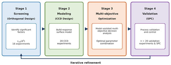
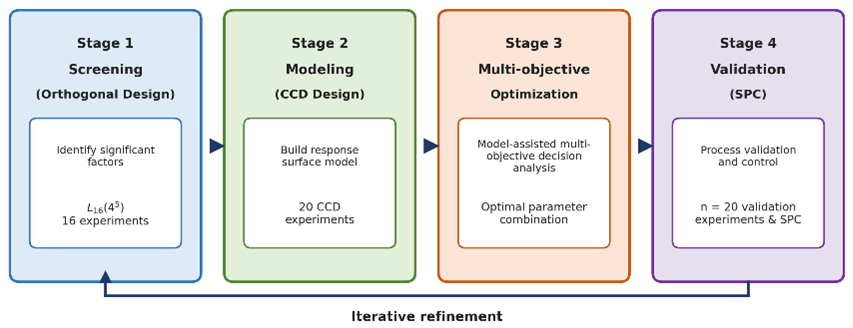
The sequential experimental design strategy follows a four-stage closed-loop logic of ‘screening-modeling-optimization-verification’, as shown in Figure 1.

Figure 1. Sequential experimental design strategy for multi-objective optimization of the RSW process.

2.3. Test Materials, Equipment, and Methods

2.3.1. Welding System and Process Parameters

The welding system comprised a Yaskawa DX100 MS80 robot (Yaskawa Electric Corporation, Kitakyushu, Japan) equipped with a medium-frequency direct-current (MFDC) inverter (1–2 kHz, current ripple < 5%). The inverter uses insulated-gate bipolar transistor (IGBT) modules (switching frequency 20 kHz, closed-loop control bandwidth 2 kHz, response time < 1 ms). The C-type welding gun has an 800 mm throat depth and electrode-arm deflection < 0.5 mm under full load. The E-16 female electrode cap has a 16 mm nominal cap body/taper diameter rather than a 16 mm working face; the spherical working face used in this study was approximately 6 mm in diameter with an R40 face radius, consistent with the ISO 5821 designation system [20]. The cap was water-cooled at ≥6 L/min with an inlet-outlet temperature difference < 5 °C. Key controller specifications are listed in Table 1.

Table 1. Key technical specifications of the welding controller.

Parameter	Value/Specification
Power input	3Φ, 380 VAC, 50/60 Hz
Rated primary-side input current	400 A (10% duty cycle; controller/transformer primary-side rating, not the secondary welding current)
Current control	MFDC, frequency 2000 Hz
Programmable pulses	Multi-pulse, max 10 stages (preheating, welding, tempering, cooling)
Current loop bandwidth	2 kHz, response < 1 ms
Force control accuracy	±2% FS (real-time feedback)

2.3.2. Material Properties and Specimen Preparation

The base materials were 1.2 mm B1500HS hot-stamped steel (0.20–0.25% C, 1.2–1.5% Mn, 0.002–0.004% B; fully lath-martensitic after hot stamping; delivery tensile strength range 1300–1700 MPa, with 1500 MPa typical) and HC340/590DP dual-phase steel (approximately 70% ferrite and 30% martensite, elongation ≥ 17%). Mechanical properties and chemical compositions are listed in Table 2.

Table 2. Mechanical properties and chemical composition of the tested materials.

Material	UTS/MPa	YS/MPa	EL/%	ν	ρ/(g/cm3)	C/%	Si/%	Mn/%	P/%	S/%	Alt/%	Cr/%	B/%	Ti/%
B1500HS	1300–1700	950–1250	≥5	0.28	7.85	0.20–0.25	≤0.40	1.2–1.5	≤0.025	≤0.010	0.01–0.06	≤0.35	≤0.005	0.02–0.05
HC340/590DP	≥590	340–440	≥17	0.30	7.85	≤0.15	≤0.60	≤2.50	≤0.040	≤0.015	≥0.010	≤0.20	—	—

Note: B1500HS tensile strength 1300–1700 MPa is the delivery performance range specified in Baosteel Q/BQB 409-2019, where 1500 MPa is the typical value (T state), yield strength 950–1250 MPa. HC340/590DP data per Baosteel Q/BQB 418-2014. ν denotes Poisson’s ratio and ρ denotes density. Composition values in Table 2 are in mass percent (wt%).

Specimen preparation: Steel plates were cut into 100 mm × 50 mm specimens by waterjet or slow wire electrical discharge machining (EDM) to avoid heat effects and spot-welded with a 35 mm overlap. Before welding, ultrasonic plus acetone cleaning was applied, with surface oil residue < 0.1 mg/m² (gravimetrically verified). Overlap-zone parallelism was controlled within ±0.05 mm (gap < 0.1 mm), and the grip-end shim thickness tolerance was ±0.02 mm, ensuring load alignment with a bending moment of <5%.

2.3.3. Performance Testing and Characterization Methods

Tensile-shear testing was performed on an XD-120B universal testing machine (accuracy class 0.5) at 5 mm/min (Shanghai Xinrenda Instrument Co., Ltd., Shanghai, China). Five specimens were tested per parameter set (n = 5). Unless stated otherwise, results are reported as mean ± standard deviation (SD); where a 95% confidence interval (CI) is used, it is calculated as mean ± t0.975, 4·s/√5. Furthermore, 1.2 mm shims were added at grip ends to ensure load alignment, reducing bending moment to <3%. Data analysis was performed using Minitab 21.4 (Minitab, LLC, State College, PA, USA) and Origin 2021 (OriginLab Corporation, Northampton, MA, USA).

In terms of macro-morphology and metallography, specimens were sectioned along the nugget center, ground, polished, and etched (4% nital), then examined under a Nikon SMZ745x stereomicroscope (Nikon Corporation, Tokyo, Japan) and an OLYMPUS GX71 metallurgical microscope (Evident Corporation (formerly Olympus), Tokyo, Japan) to measure nugget diameter and indentation depth and observe the microstructures of the nugget, HAZ, and base metal.

Scanning electron microscopy (SEM) (JEOL, Tokyo, Japan) was used to examine nugget morphology, HAZ morphology, interface appearance, and fracture surfaces. Energy-dispersive spectroscopy (EDS), electron backscatter diffraction (EBSD), and composition profile measurements were not performed; therefore, no elemental distribution or grain size claims are made from these images.

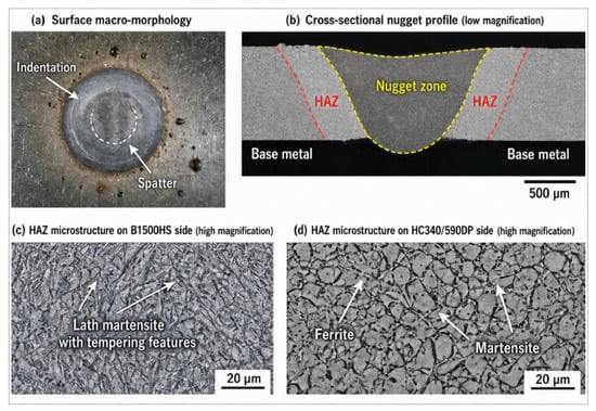
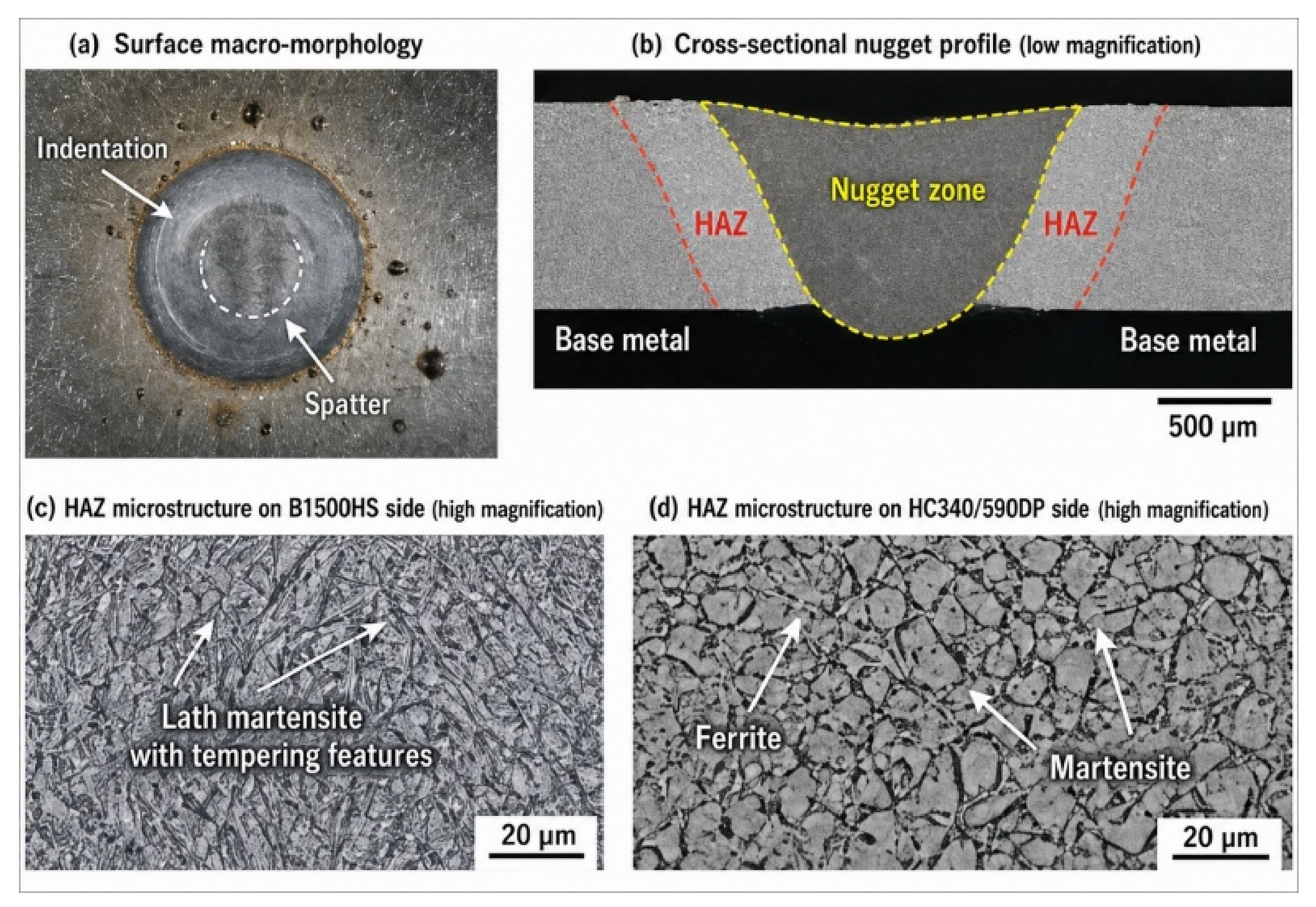
Figure 2 shows typical macro- and micro-scale characterization results of the dissimilar joint welded under representative preliminary parameters (7.5/8.0 kA, 3.0 kN, 12/15 cycles).

Figure 2. Macroscopic and microscopic morphologies of the RSW joint welded under representative preliminary parameters (7.5/8.0 kA, 3.0 kN, 12/15 cycles): (a) surface macro-morphology, with arrows identifying electrode indentation and spatter; (b) cross-sectional nugget profile, with the yellow dashed line marking the nugget boundary and red dashed lines marking the HAZ/base-metal boundaries; (c) HAZ microstructure on the B1500HS side, with arrows indicating tempered lath-martensitic features; (d) HAZ microstructure on the HC340/590DP side, with arrows identifying ferrite and martensite constituents.

3. Single-Factor Process Parameter Effects

Single-factor experiments were conducted to reveal the independent effects of welding current, electrode force, and welding time on nugget formation and joint performance.

3.1. Nonlinear Effect of Welding Current on Nugget Formation and Joint Performance

3.1.1. Logistic Growth Pattern of Nugget Diameter

The effect of welding current on nugget diameter exhibits a typical S-shaped curve [21], which can be described by the logistic model:

$$d_L={\displaystyle \frac{d_{max}}{1+ex{p}^{-\mathrm{k}\left(I-I_0\right)}}}$$

(1)

where, from nonlinear fitting of the Table 3 data, $d_{max}$ ≈ 6.3 mm is the saturation diameter; $k$ ≈ 1.2 kA⁻¹ is the growth rate; and $I_0$ ≈ 5.1 kA is the characteristic current. Below 5 kA, nugget melting is incomplete; 6–8 kA is the linear growth zone. Above 8 kA, the diameter saturates, but spatter risk rises sharply.

With electrode force fixed at 3.0 kN and the first/second weld pulse durations fixed at 12/15 cycles, the first-pulse current was varied from 4.0 to 8.5 kA, and the second-pulse current was set 0.5 kA higher. Here, “first/second pulse” denotes the weld schedule sequence, not the transformer primary/secondary sides. Results are shown in Table 3.

Table 3. Effect of weld pulse current on weld performance (electrode force 3.0 kN; first/second weld pulse durations 12/15 cycles; IF, interfacial fracture; PF, pullout failure).

No.	${\mathit{I}}_1$ (kA)	${\mathit{I}}_2$ (kA)	${\mathit{d}}_{\mathit{L}}$ (mm)	${\mathit{F}}_{\mathit{m}\mathit{a}\mathit{x}}$ (kN)	Mode
1	4.0	4.5	1.47 ± 0.12	2.23 ± 0.18	IF
2	5.0	5.5	2.67 ± 0.15	9.76 ± 0.25	IF
3	5.5	6.0	4.46 ± 0.18	10.32 ± 0.22	PF
4	6.0	6.5	4.77 ± 0.16	10.44 ± 0.24	PF
5	6.5	7.0	5.23 ± 0.20	10.46 ± 0.21	PF
6	7.0	7.5	5.37 ± 0.17	11.91 ± 0.23	PF
7	7.3	7.8	5.54 ± 0.19	12.05 ± 0.26	PF
8	7.5	8.0	6.21 ± 0.21	14.85 ± 0.28	PF
9	7.8	8.3	6.34 ± 0.23	13.53 ± 0.25	PF
10	8.0	8.5	6.26 ± 0.20	13.25 ± 0.27	PF
11	8.3	8.8	6.19 ± 0.22	13.20 ± 0.24	PF
12	8.5	9.0	6.05 ± 0.24	13.03 ± 0.29	PF

Note: Data are mean ± SD of five replicates. Table 3, Table 4 and Table 5 were acquired as independent single-factor batches. At the repeated nominal condition (7.5/8.0 kA, 3.0 kN, 12/15 cycles), the batch means were 6.21, 6.71, and 5.68 mm for nugget diameter and 14.85, 14.15, and 12.26 kN for tensile-shear force. The corresponding batch-to-batch CVs are 8.31% and 9.74%, respectively. Summary ANOVA indicates significant batch-mean offsets (nugget diameter: F = 28.20, p = 2.91 × 10⁻⁵; tensile-shear force: F = 117.22, p = 1.33 × 10⁻⁸), whereas Bartlett tests show homogeneous within-batch variances (p = 0.978 and 0.997). Therefore, factor trends are interpreted only within each batch; the repeated-condition differences are treated as a batch-effect limitation rather than measurement noise.

Table 3. Effect of weld pulse current on weld performance (electrode force 3.0 kN; first/second weld pulse durations 12/15 cycles; IF, interfacial fracture; PF, pullout failure).

No.	${\mathit{I}}_1$ (kA)	${\mathit{I}}_2$ (kA)	${\mathit{d}}_{\mathit{L}}$ (mm)	${\mathit{F}}_{\mathit{m}\mathit{a}\mathit{x}}$ (kN)	Mode
1	4.0	4.5	1.47 ± 0.12	2.23 ± 0.18	IF
2	5.0	5.5	2.67 ± 0.15	9.76 ± 0.25	IF
3	5.5	6.0	4.46 ± 0.18	10.32 ± 0.22	PF
4	6.0	6.5	4.77 ± 0.16	10.44 ± 0.24	PF
5	6.5	7.0	5.23 ± 0.20	10.46 ± 0.21	PF
6	7.0	7.5	5.37 ± 0.17	11.91 ± 0.23	PF
7	7.3	7.8	5.54 ± 0.19	12.05 ± 0.26	PF
8	7.5	8.0	6.21 ± 0.21	14.85 ± 0.28	PF
9	7.8	8.3	6.34 ± 0.23	13.53 ± 0.25	PF
10	8.0	8.5	6.26 ± 0.20	13.25 ± 0.27	PF
11	8.3	8.8	6.19 ± 0.22	13.20 ± 0.24	PF
12	8.5	9.0	6.05 ± 0.24	13.03 ± 0.29	PF

Note: Data are mean ± SD of five replicates. Table 3, Table 4 and Table 5 were acquired as independent single-factor batches. At the repeated nominal condition (7.5/8.0 kA, 3.0 kN, 12/15 cycles), the batch means were 6.21, 6.71, and 5.68 mm for nugget diameter and 14.85, 14.15, and 12.26 kN for tensile-shear force. The corresponding batch-to-batch CVs are 8.31% and 9.74%, respectively. Summary ANOVA indicates significant batch-mean offsets (nugget diameter: F = 28.20, p = 2.91 × 10⁻⁵; tensile-shear force: F = 117.22, p = 1.33 × 10⁻⁸), whereas Bartlett tests show homogeneous within-batch variances (p = 0.978 and 0.997). Therefore, factor trends are interpreted only within each batch; the repeated-condition differences are treated as a batch-effect limitation rather than measurement noise.

Table 4. Effect of electrode force on weld performance (welding current 7.5/8.0 kA, welding time 12/15 cycles).

No.	${\mathit{F}}_{\mathit{e}\mathit{l}\mathit{e}\mathit{c}}$ (kN)	${\mathit{d}}_{\mathit{L}}$ (mm)	${\mathit{F}}_{\mathit{m}\mathit{a}\mathit{x}}$ (kN)	Mode
13	1.0	4.99 ± 0.22	11.08 ± 0.31	PF
14	1.3	5.63 ± 0.19	12.01 ± 0.28	PF
15	1.5	5.65 ± 0.21	12.22 ± 0.25	PF
16	1.8	5.99 ± 0.18	12.33 ± 0.27	PF
17	2.0	6.02 ± 0.20	12.57 ± 0.24	PF
18	2.3	6.05 ± 0.19	12.69 ± 0.26	PF
19	2.5	6.08 ± 0.21	12.92 ± 0.23	PF
20	2.8	6.21 ± 0.22	14.56 ± 0.29	PF
21	3.0	6.71 ± 0.23	14.15 ± 0.27	PF
22	3.3	6.65 ± 0.24	14.12 ± 0.30	PF
23	3.5	6.41 ± 0.25	13.86 ± 0.28	PF
24	3.8	6.39 ± 0.27	13.80 ± 0.31	PF

Note: Data are mean ± standard deviation of 5 replicates. The peak tensile-shear force occurs at 2.8 kN (14.56 kN); the optimal force range is 2.8–3.0 kN, within which nugget diameter is 6.21–6.71 mm and tensile-shear force is 14.15–14.56 kN. Test 21 (3.0 kN) and Test 8 in Table 3 share the same nominal parameters (7.5/8.0 kA, 12/15 cycles) but were conducted in independent single-factor batches (Section 3.2 vs. Section 3.1). The 8.1% diameter offset (6.21 mm in Table 3 vs. 6.71 mm in Table 4) and 4.7% force offset (14.85 vs. 14.15 kN) illustrate the batch-to-batch variation quantified in the Table 3 note (CV 8.31% and 9.74%, respectively).

Table 4. Effect of electrode force on weld performance (welding current 7.5/8.0 kA, welding time 12/15 cycles).

No.	${\mathit{F}}_{\mathit{e}\mathit{l}\mathit{e}\mathit{c}}$ (kN)	${\mathit{d}}_{\mathit{L}}$ (mm)	${\mathit{F}}_{\mathit{m}\mathit{a}\mathit{x}}$ (kN)	Mode
13	1.0	4.99 ± 0.22	11.08 ± 0.31	PF
14	1.3	5.63 ± 0.19	12.01 ± 0.28	PF
15	1.5	5.65 ± 0.21	12.22 ± 0.25	PF
16	1.8	5.99 ± 0.18	12.33 ± 0.27	PF
17	2.0	6.02 ± 0.20	12.57 ± 0.24	PF
18	2.3	6.05 ± 0.19	12.69 ± 0.26	PF
19	2.5	6.08 ± 0.21	12.92 ± 0.23	PF
20	2.8	6.21 ± 0.22	14.56 ± 0.29	PF
21	3.0	6.71 ± 0.23	14.15 ± 0.27	PF
22	3.3	6.65 ± 0.24	14.12 ± 0.30	PF
23	3.5	6.41 ± 0.25	13.86 ± 0.28	PF
24	3.8	6.39 ± 0.27	13.80 ± 0.31	PF

Note: Data are mean ± standard deviation of 5 replicates. The peak tensile-shear force occurs at 2.8 kN (14.56 kN); the optimal force range is 2.8–3.0 kN, within which nugget diameter is 6.21–6.71 mm and tensile-shear force is 14.15–14.56 kN. Test 21 (3.0 kN) and Test 8 in Table 3 share the same nominal parameters (7.5/8.0 kA, 12/15 cycles) but were conducted in independent single-factor batches (Section 3.2 vs. Section 3.1). The 8.1% diameter offset (6.21 mm in Table 3 vs. 6.71 mm in Table 4) and 4.7% force offset (14.85 vs. 14.15 kN) illustrate the batch-to-batch variation quantified in the Table 3 note (CV 8.31% and 9.74%, respectively).

Table 5. Effect of welding time on weld performance (welding current 7.5/8.0 kA, electrode force 3.0 kN).

No.	${\mathit{t}}_1$ (cyc)	${\mathit{t}}_2$ (cyc)	${\mathit{d}}_{\mathit{L}}$ (mm)	${\mathit{F}}_{\mathit{m}\mathit{a}\mathit{x}}$ (kN)	Mode
25	2	5	3.76 ± 0.18	9.21 ± 0.25	PF
26	4	7	4.99 ± 0.19	9.64 ± 0.28	PF
27	6	9	5.00 ± 0.21	11.22 ± 0.24	PF
28	8	11	5.01 ± 0.20	11.33 ± 0.27	PF
29	10	13	5.48 ± 0.22	11.58 ± 0.26	PF
30	11	14	5.48 ± 0.23	11.86 ± 0.25	PF
31	12	15	5.68 ± 0.21	12.26 ± 0.28	PF
32	13	16	6.21 ± 0.24	14.88 ± 0.30	PF
33	14	17	6.20 ± 0.25	14.11 ± 0.29	PF
34	16	19	6.08 ± 0.23	13.64 ± 0.31	PF
35	18	21	5.93 ± 0.26	13.14 ± 0.32	PF
36	20	23	5.85 ± 0.27	12.97 ± 0.34	PF

Note: Data are mean ± standard deviation of five replicates. Optimal time combination is 13/16 cycles, with measured HAZ width of 0.67 ± 0.08 mm.

Table 5. Effect of welding time on weld performance (welding current 7.5/8.0 kA, electrode force 3.0 kN).

No.	${\mathit{t}}_1$ (cyc)	${\mathit{t}}_2$ (cyc)	${\mathit{d}}_{\mathit{L}}$ (mm)	${\mathit{F}}_{\mathit{m}\mathit{a}\mathit{x}}$ (kN)	Mode
25	2	5	3.76 ± 0.18	9.21 ± 0.25	PF
26	4	7	4.99 ± 0.19	9.64 ± 0.28	PF
27	6	9	5.00 ± 0.21	11.22 ± 0.24	PF
28	8	11	5.01 ± 0.20	11.33 ± 0.27	PF
29	10	13	5.48 ± 0.22	11.58 ± 0.26	PF
30	11	14	5.48 ± 0.23	11.86 ± 0.25	PF
31	12	15	5.68 ± 0.21	12.26 ± 0.28	PF
32	13	16	6.21 ± 0.24	14.88 ± 0.30	PF
33	14	17	6.20 ± 0.25	14.11 ± 0.29	PF
34	16	19	6.08 ± 0.23	13.64 ± 0.31	PF
35	18	21	5.93 ± 0.26	13.14 ± 0.32	PF
36	20	23	5.85 ± 0.27	12.97 ± 0.34	PF

Note: Data are mean ± standard deviation of five replicates. Optimal time combination is 13/16 cycles, with measured HAZ width of 0.67 ± 0.08 mm.

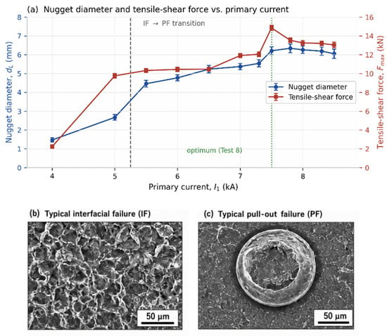
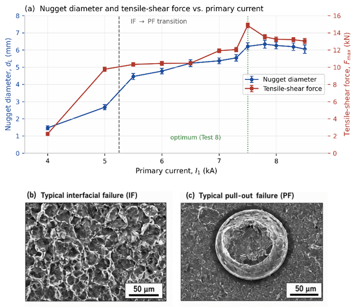
Table 3 shows that below 5.5 kA, insufficient heat input causes interfacial fracture (IF); at 5.5 kA, the nugget meets the requirement (d_L > 3.8 mm) and the fracture mode transitions to the desirable pullout failure (PF). From 7.5 kA (Test 8) to 8.0 kA (Test 10), nugget diameter rises only 0.8% (6.21 → 6.26 mm), whereas tensile-shear force drops 10.8% (14.85 → 13.25 kN), confirming that 7.5 kA is near-optimal and further current increase rapidly degrades performance. The optimal process window is narrow (approximately 7.5 ± 0.2 kA) (Figure 3).

Figure 3. Single-factor effect of welding current on weld performance and fracture mode transition: (a) nugget diameter and tensile-shear force versus first-pulse current; (b) typical IF fracture surface (SEM); (c) typical PF fracture surface (SEM, button type).

3.1.2. Current Waveform and Secondary Pulse Mechanism

Current waveform optimization: Conventional square-wave current has a 10–90% rise time of <2 ms and readily produces impact spatter; sinusoidal or trapezoidal waveforms (rise time 5–8 ms) significantly improve this [22].

The secondary pulse ($I_2$) primarily functions for ‘shaping’ and ‘supplemental heating’. The $I_2/I_1$ ratio is key, recommended at 1.05–1.10. An excessive ratio (>1.15$I_1$) overheats the nugget and coarsens columnar grains; an insufficient ratio (<1.05$I_1$) provides inadequate heating and incomplete edge fusion. The secondary time ratio $t_2/t_1$ is recommended at 1.2–1.4; excessive duration causes HAZ expansion.

3.1.3. Critical Conditions for Fracture Mode Transition

The critical nugget diameter for interfacial fracture (IF) to pullout failure (PF) transition [23] follows the relationship with sheet thickness δ:

$$d_c\approx 3.5\sqrt{\delta }$$

(2)

Here, dc is the critical transition nugget diameter (mm), and δ is the sheet thickness (mm). For a 1.2 mm sheet, the critical transition diameter is approximately 3.8–4.2 mm; with an engineering safety margin, 4.0–4.5 mm is adopted as the control target. The IF-to-PF transition is assessed from the measured nugget diameter and observed fracture mode; no independent hardness threshold is inferred.

The single-factor current effects establish the baseline process window. The following section examines the competitive mechanism of electrode force, which simultaneously governs contact resistance and heat dissipation.

3.2. Competitive Mechanism of Electrode Force on Contact Resistance and Heat Dissipation

3.2.1. Holm Contact Theory

The effect of electrode force on contact resistance follows Holm contact theory [4], with experimental validation in copper systems reported elsewhere [24]:

$$R_{\mathrm{contact}}={\displaystyle \frac{{\rho }_1+{\rho }_2}{4a}}+{\displaystyle \frac{{\rho }_s}{\pi a^2}}$$

(3)

where Rcontact is the contact resistance (Ω); ρ1 and ρ2 are the resistivities of the two contacting bodies (Ω·m); a is the effective contact-spot radius (m); and ρs is the surface-film resistivity (Ω·m²). For elastic Hertzian contact, a ∝ F1/3. Consequently, the constriction term (ρ1 + ρ2)/(4a) scales approximately as F − 1/3, whereas the film term ρs/(πa²) scales approximately as F − 2/3; an exponential force dependence is not implied by Holm theory [4]. Increasing electrode force therefore lowers interfacial heat generation while increasing electrode-sheet heat conduction, producing competing effects on nugget formation.

With welding current (first pulse 7.5 kA, second pulse 8.0 kA) and welding time (12/15 cycles) fixed, electrode force was varied from 1.0 to 3.8 kN. Results are shown in Table 4.

3.2.2. Force-HAZ Softening-Strength Compensation Mechanism

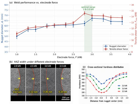
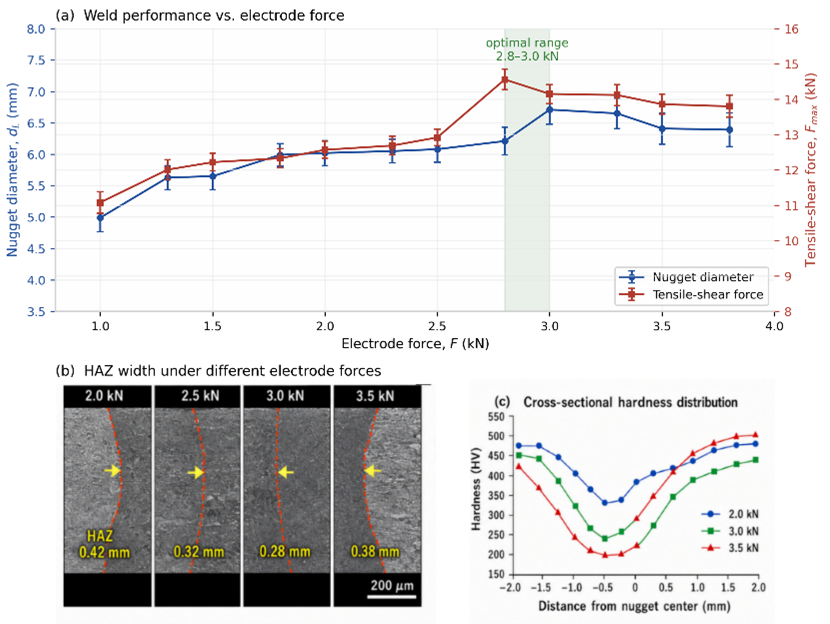
Table 4 shows that the effect of electrode force on the two metrics is asymmetric: from 2.5 to 3.5 kN, nugget diameter increases by 5.4%, whereas the HAZ response and hardness loss reduce the effective load-bearing section [25,26,27]. Figure 4c is a Vickers microhardness profile (HV0.5, 0.5 kgf nominal load) [26,27], not nanoindentation. The chart indicates outer-region hardness of approximately 460–510 HV and local minima of approximately 240 HV at 3.0 kN and 190 HV at 3.5 kN, rather than a uniform decrease from 380 to 310 HV. For a conceptual section-based illustration, the effective bearing force is expressed as

$$F_{eff}={\sigma }_{weld}·A_{weld}·{\eta }_{aspect}+{\sigma }_{HAZ}·A_{HAZ}+{\sigma }_{BM}·A_{BM}$$

(4)

where ${\eta }_{aspect}$ is a depth-to-diameter correction coefficient (${\eta }_{aspect}$ = 0.8 + 0.4 × depth-to-diameter ratio); A_weld, A_HAZ, and A_BM are the effective nugget, softened HAZ, and base-metal load-bearing sections; and σ_weld, σ_HAZ, and σ_BM are the corresponding representative strengths. Equation (4) is a conceptual section estimate used to explain the competition between nugget enlargement and HAZ softening; no numerical values are assigned to the constituent terms, and it is not a fitted constitutive model.

Figure 4. Competitive mechanism of electrode force on contact resistance and HAZ softening: (a) weld performance versus electrode force; (b) HAZ width under different electrode forces, with dashed lines marking the HAZ boundaries; (c) cross-sectional Vickers microhardness profiles, showing force-dependent local hardness minima in the softened HAZ.

Figure 4 shows the nugget size, HAZ width, and hardness distribution under different electrode forces.

3.3. Effect of Welding Time on Nugget Growth and HAZ Softening

3.3.1. Heat Balance Equation and Energy Accumulation Pattern

The effect of welding time can be interpreted using a lumped RSW heat balance relation [28]. Joule heating supplies the nugget formation energy, while conduction into the sheets and electrodes limits the usable heat. A simplified ideal energy balance gives the scaling relation:

$$d_L^3=K·{\displaystyle \frac{\beta \eta I^2{R}_{\mathrm{contact}}t}{\pi \rho c_p{T}_n}}$$

(5)

where β is a dimensionless contact-geometry correction coefficient, η is thermal efficiency, R_contact is contact resistance, ρ is material density, c_p is specific heat capacity, and T_n is nugget temperature. Because time-dependent contact resistance, temperature fields, and heat losses were not measured, Equation (5) is not fitted and is not used to calculate the reported diameters. It serves only to explain why nugget growth initially increases with time and then saturates as heat dissipation becomes dominant.

With welding current (7.5/8.0 kA) and electrode force (3.0 kN) fixed, welding time was varied (first pulse 2–20 cycles, second pulse +3 cycles); results are shown in Table 5.

Table 5 shows that both responses initially increased with welding time, peaked at 13/16 cycles, and then declined as continued heat input changed the balance between interfacial heat generation and heat dissipation. The post-peak decrease was accompanied by greater indentation and HAZ tempering; no grain-coarsening kinetics are inferred from the available micrographs.

3.3.2. Tempering Parameter and HAZ Softening Quantitative Relationship

The increase in HAZ width and hardness loss with welding time is consistent with carbide precipitation and martensite tempering during the rapid thermal cycle [29]. However, the actual HAZ thermal cycle temperature was not measured, and a tempering parameter was not fitted. The empirical upper limit of 15 cycles (300 ms) for the first pulse is therefore specific to the present joint, thickness, electrode geometry, and equipment rather than a general metallurgical threshold.

3.4. Multi-Scale Competition Mechanism and Joint-Specific HAZ Screening Envelope

The single-factor data in Section 3.1, Section 3.2 and Section 3.3 reveal a competition among nugget diameter, tensile-shear force, and HAZ softening. Increasing electrode force promotes nugget growth (Table 4: 6.21 mm at 2.8 kN versus 6.71 mm at 3.0 kN) but also produces deeper HAZ hardness minima (Figure 4c), so tensile-shear force decreases beyond 3.0 kN. This non-monotonic behavior supports including HAZ integrity as a third screening dimension. On the basis of the measured HAZ widths, microhardness profiles, failure modes, and mechanical responses, a joint-specific descriptive screening envelope of HAZ width < 0.7 mm and hardness loss < 50% is proposed for this 1.2 mm B1500HS/HC340/590DP joint and the present equipment. The 0.7 mm threshold is a rounded engineering bound near the observed optimal window response (Table 5: 0.67 ± 0.08 mm at 13/16 cycles). The 50% hardness loss limit is derived from the Vickers microhardness profiles in Figure 4c (local minimum ~240 HV versus outer-region hardness ~460–510 HV at 3.0 kN, i.e., an approximately 48–53% loss); because this limit lies within the scatter of the data used to derive it, it is presented as a descriptive envelope without an explicit engineering margin. At 3.5 kN, the joint clearly violates this bound (~190 HV, ~58–63% loss). This envelope was never applied to the selected 13/17-cycle validation condition (Section 4.5) because HAZ width and microhardness were not measured on the n = 20 validation sample; it therefore remains conditional on the single-factor HAZ data in Section 3.2 and Section 3.3. This envelope is an engineering screening description, not an extension of ISO 10447 or ISO 14273 and not a general material-independent limit. No EBSD, nanoindentation, Hall-Petch, or quantitative microstructure-property fit was performed; such correlations require future site-specific microstructure and local-property measurements.

4. Multi-Parameter Optimization and Verification

4.1. Orthogonal Experimental Design and Range Analysis

4.1.1. $L_{16}\left(4^5\right)$ Orthogonal Array and Factor Levels

An $L_{16}\left(4^5\right)$ orthogonal array was used to study the effects of five four-level factors (first-pulse current A, second-pulse current B, electrode force C, first-pulse time D, second-pulse time E) on nugget diameter ($d_L$) and tensile-shear force ($F_{\max }$). Each trial was repeated three times, yielding 48 raw datasets. Sequential strategies have proven effective in balancing experimental efficiency and model precision in welding optimization [30]. Factor levels are shown in Table 6.

Table 6. Factor levels of the $L_{16}\left(4^5\right)$ orthogonal experiment.

Level	A: ${\mathit{I}}_1$/kA	B: ${\mathit{I}}_2$/kA	C: ${\mathit{F}}_{\mathit{e}\mathit{l}\mathit{e}\mathit{c}}$/kN	D: ${\mathit{t}}_1$/cyc	E: ${\mathit{t}}_2$/cyc
1	7.5	8.0	2.8	13	16
2	7.8	8.3	3.0	14	17
3	8.0	8.5	3.3	16	19
4	8.3	8.8	3.5	18	21

Note: Cycle represents power cycles, 1 cycle = 20 ms (50 Hz power supply). Level selection is based on preliminary experiments and engineering experience, covering the reasonable range of the process window.

The 48 sets of raw experimental data were averaged within groups, with 16 group statistical summaries shown in Table 7.

Table 7. Within-group statistical summary of the orthogonal experiment (means of 16 runs).

Run	A	B	C	D	E	${\mathit{d}}_{\mathit{L}}$ (mm)	${\mathit{F}}_{\mathbf{max}}$ (kN)	Mode
1	7.5	8.0	2.8	13	16	6.27 ± 0.06	14.02 ± 0.22	PF
2	7.5	8.3	3.0	14	17	6.75 ± 0.18	13.49 ± 0.15	PF
3	7.5	8.5	3.3	16	19	6.15 ± 0.19	14.18 ± 0.16	PF
4	7.5	8.8	3.5	18	21	6.01 ± 0.21	11.97 ± 0.21	PF
5	7.8	8.0	3.0	16	21	6.72 ± 0.11	14.65 ± 0.13	PF
6	7.8	8.3	2.8	18	19	6.66 ± 0.23	14.47 ± 0.27	PF
7	7.8	8.5	3.5	13	17	6.50 ± 0.17	14.83 ± 0.08	PF
8	7.8	8.8	3.3	14	16	6.42 ± 0.13	14.96 ± 0.24	PF
9	8.0	8.0	3.3	18	17	5.98 ± 0.18	14.60 ± 0.15	PF
10	8.0	8.3	3.5	16	16	5.72 ± 0.17	14.99 ± 0.15	PF
11	8.0	8.5	2.8	14	21	6.77 ± 0.08	15.14 ± 0.30	PF
12	8.0	8.8	3.0	13	19	6.95 ± 0.10	14.15 ± 0.27	PF
13	8.3	8.0	3.5	14	19	5.94 ± 0.31	14.41 ± 0.14	PF
14	8.3	8.3	3.3	13	21	6.18 ± 0.18	13.02 ± 0.26	PF
15	8.3	8.5	3.0	18	16	6.14 ± 0.15	13.77 ± 0.12	PF
16	8.3	8.8	2.8	16	17	6.59 ± 0.15	13.69 ± 0.15	PF

Note: Data are mean ± standard deviation of three replicates. PF indicates pullout failure. Total degrees of freedom = 47, factor degrees of freedom = 15, error degrees of freedom = 32 (16 groups × (3 − 1)).

4.1.2. Within-Group Statistics and Range Analysis

Based on the 48 sets of raw data, the mean values and ranges for each factor level were calculated, with results shown in Table 8.

Table 8. Range analysis results of the orthogonal experiment (n = 3, based on 48 raw data points).

Response	Stat.	A	B	C	D	E
dl	k1	6.295	6.228	6.573	6.474	6.136
	k2	6.573	6.328	6.642	6.472	6.454
	k3	6.354	6.389	6.179	6.293	6.425
	k4	6.213	6.492	6.042	6.197	6.421
	R	0.360	0.264	0.599	0.277	0.318
	Opt.	A2	B4	C2	D1	E2
	Order	C > A > E > D > B
Fl	k1	13.414	14.421	14.330	14.007	14.433
	k2	14.727	13.993	14.014	14.499	14.152
	k3	14.723	14.481	14.192	14.378	14.304
	k4	13.722	13.691	14.049	13.702	13.696
	R	1.313	0.788	0.315	0.798	0.740
	Opt.	A2	B3	C1	D2	E1
	Order	A > D > B > E > C

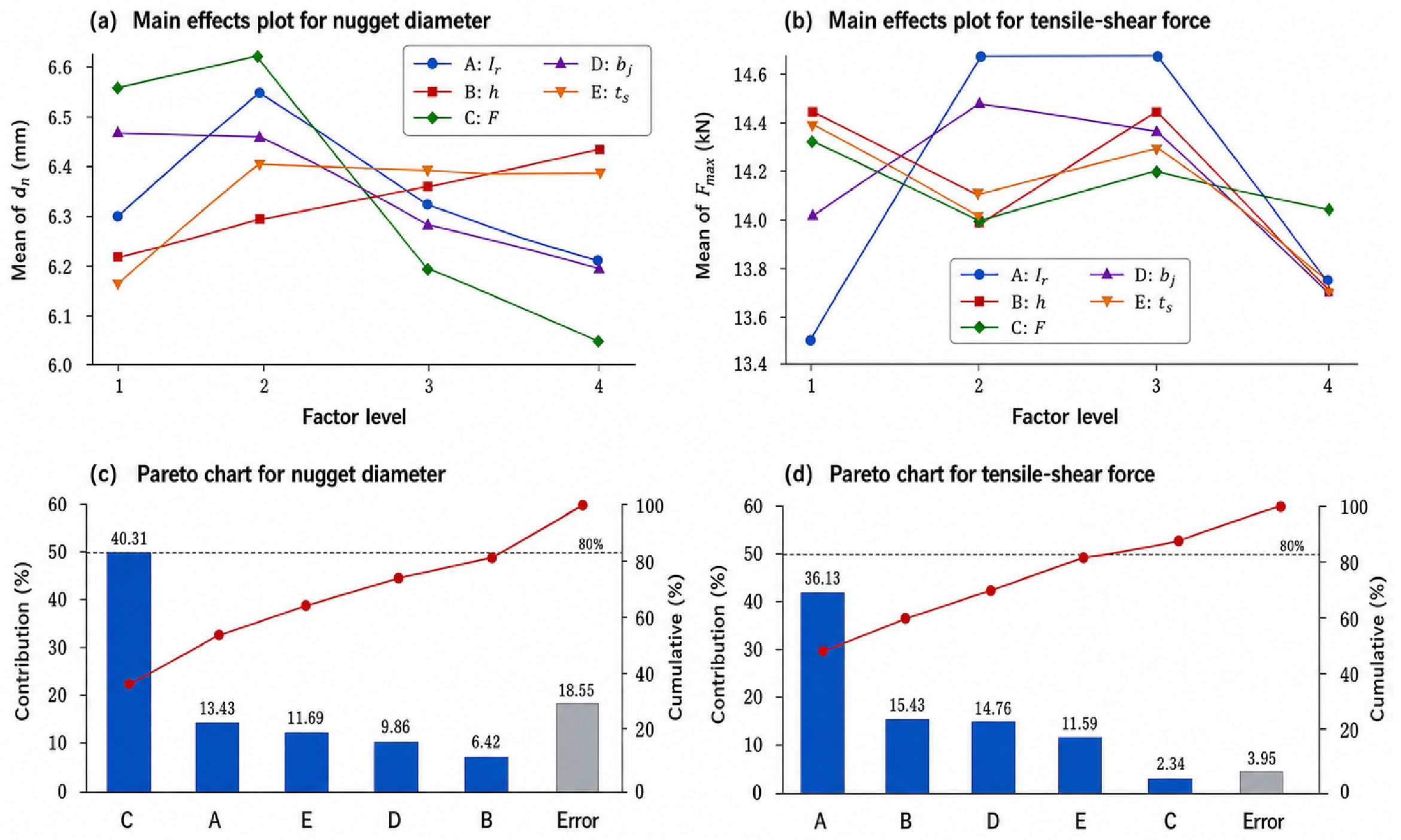
Electrode force C has the greatest effect on nugget diameter (R = 0.599 mm), while first-pulse current A dominates tensile-shear force (R = 1.313 kN). The factor importance order is C > A > E > D > B for nugget diameter and A > D > B > E > C for tensile-shear force. The optimal levels conflict (A₂B₄C₂D₁E₂ for nugget diameter vs. A₂B₃C₁D₂E₁ for tensile-shear force), requiring coordination through comprehensive scoring or response surface methodology.

4.2. Analysis of Variance (ANOVA) and Significance Testing

Within the orthogonal batch, 48 observations (16 conditions × 3 replicates) were analyzed by ANOVA at α = 0.05, with critical values F0.05(3,32) = 2.90 and F0.01(3,32) = 4.46. The analysis decomposes variance within this batch only; it is not pooled across the three independent single-factor batches because those batches show significant mean offsets at the repeated nominal condition (Table 3 note). Results are shown in Table 9.

Table 9. Results of analysis of variance (ANOVA) (based on 48 raw data points).

Resp.	Source	SS	df	MS	F	Sig.	Contr.%
$d_L$	A	0.855	3	0.285	9.12	**	12.43
	B	0.442	3	0.147	4.71	**	6.42
	C	3.097	3	1.032	33.01	**	45.03
	D	0.679	3	0.227	7.24	**	9.88
	E	0.804	3	0.268	8.57	**	11.69
	Err	1.001	32	0.031	--	--	14.55
	Tot	6.879	47	--	--	--	100
$F_{\max }$	A	16.622	3	5.541	139.50	**	51.73
	B	5.021	3	1.674	42.14	**	15.63
	C	0.752	3	0.251	6.31	**	2.34
	D	4.742	3	1.581	39.81	**	14.76
	E	3.723	3	1.241	31.26	**	11.59
	Err	1.271	32	0.040	--	--	3.95
	Tot	32.131	47	--	--	--	100

Note: ** indicates p < 0.01 (highly significant), * indicates 0.01 ≤ p < 0.05 (significant), ns indicates p ≥ 0.05 (not significant). Percentage contribution = $S{S}_{factor}$/$S{S}_{total}$ × 100%. Sum of squares calculated based on 48 raw data points (16 groups × 3 replicates); error estimation uses within-group variance.

For nugget diameter, the within-batch variance shares are 45.03% for electrode force C (F = 33.01, p < 0.01) and 12.43% for first-pulse current A (F = 9.12, p < 0.01). For tensile-shear force, first-pulse current A is dominant (51.73%, F = 139.50), followed by second-pulse current B (15.63%), first-pulse time D (14.76%), and second-pulse time E (11.59%); electrode force C contributes only 2.34% (F = 6.31, p < 0.01). These percentages are within-batch variance decomposition shares, not independent confirmation of the single-factor batches. The contrast between a large C effect on diameter and a small C effect on force is consistent with the force-HAZ softening-load-bearing competition discussed qualitatively using Equation (4).

It must be noted that the error term in Table 9 is derived from within-group replication (n = 3) within the single orthogonal batch and therefore reflects only measurement uncertainty and short-range random variation under fixed experimental conditions. The batch-to-batch offsets observed at the repeated nominal condition across the three independent single-factor batches (Table 3 note: CV 8.31% for nugget diameter and 9.74% for tensile-shear force) indicate the presence of batch-to-batch systematic variation that is not captured by the within-batch error term. Consequently, the F statistics and significance markers in Table 9 should be interpreted as descriptive rankings of factor importance within this specific batch, rather than as confirmatory evidence of reproducible batch-to-batch effects. A random-effects or mixed-model analysis incorporating batch as a blocking factor would be required for batch-to-batch generalization, which is beyond the scope of the present fixed-effects design.

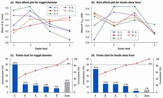
Figure 5 visualizes the range analysis and ANOVA results for direct comparison of factor significance on the two metrics.

Figure 5. Range analysis and ANOVA results of the orthogonal experiment: (a) main effect plot for nugget diameter; (b) main effect plot for tensile-shear force; (c) Pareto chart for nugget diameter; (d) Pareto chart for tensile-shear force.

4.3. Response Surface Model Based on Central Composite Design

4.3.1. CCD Design Matrix and Coded Variables

Phase I screening used the $L_{16}\left(4^5\right)$ orthogonal experiment. Range analysis gives the nugget-diameter factor order C (electrode force) > A (first-pulse current) > E (second-pulse time) > D (first-pulse time) > B (second-pulse current). Within-batch ANOVA gives variance shares of 45.03% for C and 12.43% for A.

Phase II uses response-specific factor subsets rather than forcing one CCD to retain the same factors for both responses. For nugget diameter, A, C, and D are retained; E is fixed because it is strongly coupled with D in the two-pulse schedule, and B has the smallest nugget diameter contribution. For tensile-shear force, A, B, D, and E are retained because they account for the dominant within-batch variance, whereas C contributes only 2.34% and is fixed near the screening optimum. This explains the intentional asymmetry between the three-factor nugget-diameter CCD and the four-factor tensile-shear CCD. Table 10 reports the nugget diameter design matrix and results. The complete 30-run tensile-shear CCD worksheet is not included in the present dataset and was unavailable for independent recalculation; Equation (7) is therefore treated as an auxiliary local calibration rather than a globally validated response surface.

Table 10. CCD design matrix and experimental results (nugget diameter model, three factors).

No.	x1	x3	x4	${\mathit{I}}_1$/kA	F/kN	${\mathit{t}}_1$/cyc	${\mathit{d}}_{\mathit{L}}$ (mm)
1	−1	−1	−1	7.50	2.80	11	5.98 ± 0.18
2	+1	−1	−1	7.80	2.80	11	6.42 ± 0.21
3	−1	+1	−1	7.50	3.50	11	5.85 ± 0.19
4	+1	+1	−1	7.80	3.50	11	6.15 ± 0.20
5	−1	−1	+1	7.50	2.80	14	6.08 ± 0.17
6	+1	−1	+1	7.80	2.80	14	6.45 ± 0.22
7	−1	+1	+1	7.50	3.50	14	5.92 ± 0.16
8	+1	+1	+1	7.80	3.50	14	6.21 ± 0.23
9	−1.682	0	0	7.40	3.15	12.5	5.72 ± 0.15
10	+1.682	0	0	7.90	3.15	12.5	6.38 ± 0.24
11	0	−1.682	0	7.65	2.56	12.5	6.28 ± 0.19
12	0	+1.682	0	7.65	3.74	12.5	5.95 ± 0.18
13	0	0	−1.682	7.65	3.15	9.98	5.89 ± 0.20
14	0	0	+1.682	7.65	3.15	15.02	6.15 ± 0.21
15	0	0	0	7.65	3.15	12.5	6.52
16	0	0	0	7.65	3.15	12.5	6.48
17	0	0	0	7.65	3.15	12.5	6.55
18	0	0	0	7.65	3.15	12.5	6.50
19	0	0	0	7.65	3.15	12.5	6.53
20	0	0	0	7.65	3.15	12.5	6.49

Note: Trials 1–8 are factorial points (2³ = 8 runs), trials 9–14 are axial points (α = 1.682), and trials 15–20 are center point replicates (n = 6, for estimating pure error).

4.3.2. Second-Order Regression Model for Nugget Diameter

For the nugget diameter CCD, the dimensionless coded variables are x1 = (I1 − 7.65)/0.15, x3 = (F − 3.15)/0.35, and x4 = (t1 − 12.5)/1.5, where I1 is first-pulse current (kA), F is electrode force (kN), and t1 is first-pulse time (cycles). A quadratic model was fitted by least squares to the 20-run matrix in Table 10 [31]:

$$d_L=6.509+0.184x_1-0.099x_3+0.051x_4-0.143x_1^2-0.120x_3^2-0.153x_4^2-0.028x_1{x}_3-0.010x_1{x}_4$$

(6)

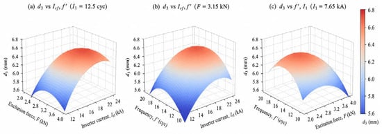
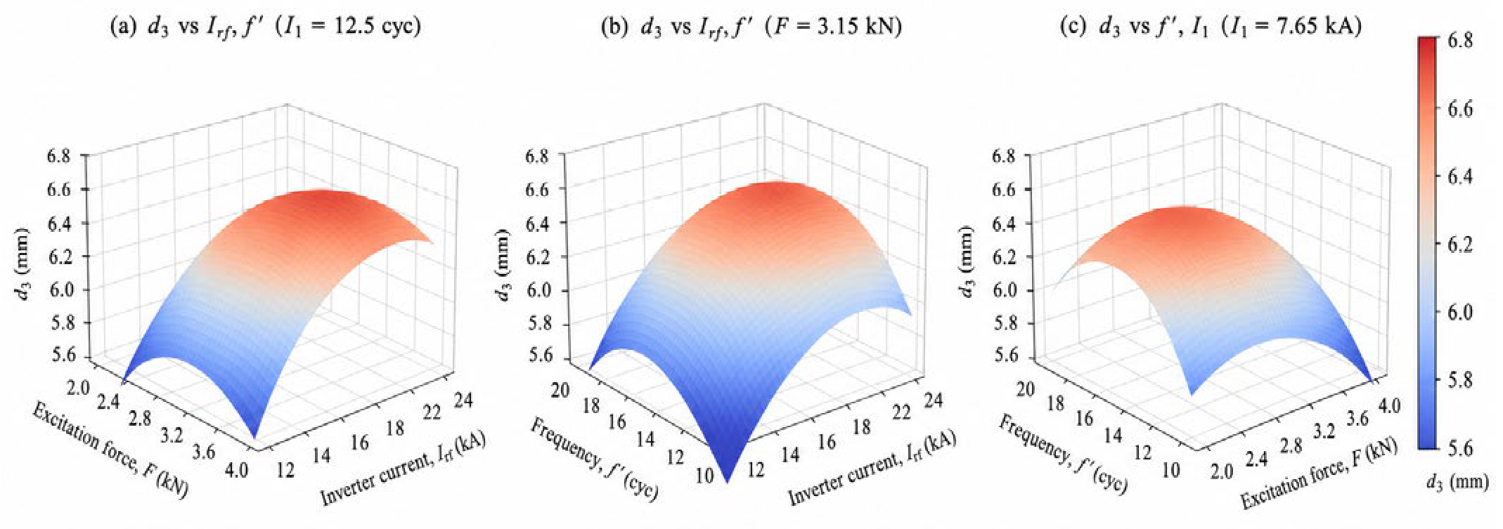
Figure 6 plots the second-order response surfaces of Equation (6). The nugget diameter forms a typical downward-opening paraboloid in the ${\mathrm{I}}_1-\mathrm{F}$ plane (Figure 6a). The stationary point of Equation (6) is located at ${\mathrm{I}}_1\approx 7.75 \mathrm{kA}$, $\mathrm{F}\approx 2.98 \mathrm{kN}$, and ${\mathrm{t}}_1\approx 12.7 \mathrm{cycles}$; the quadratic effect of ${\mathrm{t}}_1$ (−0.153) makes the response surface steeper along the time axis (Figure 6b), while excessive electrode force significantly suppresses nugget growth (Figure 6c).

Figure 6. Second-order response surfaces of nugget diameter: (a) nugget diameter versus first-pulse current and electrode force (first-pulse time 12.5 cycles); (b) nugget diameter versus first-pulse current and first-pulse time (electrode force 3.15 kN); (c) nugget diameter versus electrode force and first-pulse time (first-pulse current 7.65 kA).

The lack-of-fit statistic reported here (FLOF = 11.28, p = 0.009) replaces an earlier calculational error (F = 2.15, p = 0.18); the original value was obtained from an incorrect error-term partition and is hereby retracted. Model calibration and point-wise check: R² = 0.969, adjusted R² = 0.941. Leave-one-out cross-validation gives a predicted R² = 0.781 (a representative 5-fold split: 0.745). The lack-of-fit test resulted in FLOF= 11.28, p = 0.009 < 0.05 (statistically significant relative to the small center-point pure error). Because lack of fit is significant, Equation (6) is used for local interpolation and trend interpretation only; it is not a globally validated predictor. The n = 20 confirmation experiment in Section 4.5 validates the selected operating point, not the full response surface. Since predicted R² is below 0.90, small-sample extrapolation carries some uncertainty; validation experiments are recommended for fine-tuning in practice.

The mean measured nugget diameter at the center points (trials 15–20) was 6.51 mm, deviating only 0.003 mm from the regression constant (6.509 mm)—negligible versus the experimental uncertainty (±0.25 mm)—confirming constant-term calibration at the center point.

4.3.3. Second-Order Regression Model for Tensile-Shear Force

The tensile-shear force relationship was originally fitted as a four-factor CCD in A, B, D, and E (16 factorial points, 8 axial points with α = 2.0, and 6 center-point replicates). The coded variables are dimensionless linear transformations, with x1, x2, x4, and x5 corresponding to A, B, D, and E, respectively. Regression terms in Equation (7) were selected by backward elimination. However, the complete 30-run design matrix and raw responses are not included in the manuscript and were unavailable for independent recalculation. Equation (7) is therefore used only as an auxiliary local calibration near the selected operating point, not as a globally validated response surface.

The local tensile-shear calibration is shown in Equation (7); the retained quadratic and interaction terms are consistent with the need for a second-order local approximation in multi-objective RSW studies [16].

$$F_{max}=14.38+0.312x_1+0.148x_2-0.095x_4-0.102x_5-0.238x_1^2-0.108x_2^2-0.065x_4^2+0.092x_1{x}_2$$

(7)

Within its calibrated neighborhood, Equation (7) has a positive x₁x₂ interaction coefficient, suggesting a local synergistic effect of the two current pulses, and a negative linear x₅ coefficient, indicating that excessive second-pulse time can degrade mechanical performance. These signs are local model interpretations rather than independent mechanistic proof.

The originally reported in-sample statistics were R² = 0.971, adjusted R² = 0.961, predicted R² = 0.938, and a non-significant lack-of-fit test (FLOF = 1.38, p = 0.31). Because the underlying 30-run worksheet is unavailable for audit, these statistics are reported as model history information and are not treated as independent validation. The validation experiment in Section 4.5 tests only the selected operating point.

4.4. Model-Assisted Multi-Objective Decision Methods

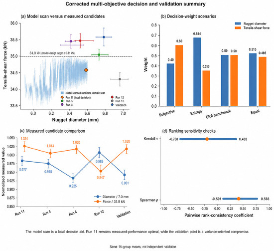
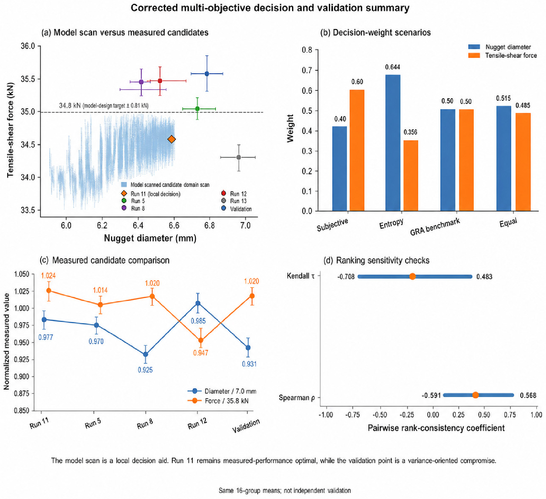
Equations (6) and (7) were used for a model-assisted candidate scan over the reported coded domain, in which Equation (7) serves strictly as an auxiliary local calibration rather than a validated response surface. Because Equation (7) underpredicts the measured validation response and its attainable coded-domain maximum is below the measured value, the scan is not interpreted as an experimentally verified Pareto frontier. Final selection therefore combines the measured orthogonal responses, model-based local interpolation, and decision weight sensitivity checks (Figure 7).

Figure 7. Statistically informed multi-objective decision summary: (a) model-assisted coded-domain response scan, measured candidates, and the validation point; the scan is not an experimentally verified Pareto frontier; (b) subjective, entropy, equal-weight GRA benchmark, and final decision weights; (c) measured nugget diameter and tensile-shear force for the leading orthogonal candidates and validation compromise; (d) rank-consistency indicators used as sensitivity checks rather than independent validation.

4.4.1. Engineering Decision Method Based on Subjective Weighting

For the subjective weighting scenario, structural load-bearing safety is prioritized (tensile-shear force weight 60%), followed by dimensional compliance (nugget diameter weight 40%) [32]. The weighted normalized objective function is

$$Y_{\mathrm{subjective}}=0.40·{\displaystyle \frac{d_L}{7.0}}+0.60·{\displaystyle \frac{F_{\max }}{15.0}}$$

(8)

Here, 7.0 mm is a normalization reference obtained by rounding the observed orthogonal maximum of 6.95 mm (Run 12, Table 7) upward. The 15.0 kN value is an empirical normalization reference from the observed high-performance region; it is not 95% of the base-material bearing capacity and is not a product specification. The subjective-weighting candidate is I1 = 7.8 kA, I2 = 8.5 kA, F = 3.0 kN, t1 = 13 cycles, and t2 = 17 cycles. This candidate is a model-assisted interpolation, not an actual orthogonal-level combination.

4.4.2. Objective Weighting Based on Entropy Method

To test sensitivity to the subjective weights, information entropy weighting was applied to the 16 orthogonal group means [33]. This calculation uses group means, whereas the ANOVA uses all 48 within-batch observations; the two analyses therefore address different questions. Min-Max normalization was applied as follows:

$$x_{ij}^{\mathsf{*}}={\displaystyle \frac{x_{ij}-\min \left(x_j\right)}{\max \left(x_j\right)-\min \left(x_j\right)}}$$

(9)

where x_ij is the original group-mean value of indicator j for run i, and x^*_ij is its Min-Max normalized value (i = 1, …, 16 runs; j = 1, 2, denoting nugget diameter and tensile-shear force, respectively). The information entropy e_j of the j-th indicator is calculated as follows:

$$e_j=-k{\sum }_{i=1}^{16}{p}_{ij}\ln p_{ij},k={\displaystyle \frac{1}{\ln 16}},p_{ij}={\displaystyle \frac{x_{ij}^{\mathsf{*}}}{{{\displaystyle \sum }}_{i=1}^{16}{x}_{ij}^{\mathsf{*}}}}$$

(10)

where p_ij = x^*_ij/Σ_ix^*_ij is the proportion of run i under indicator j; when p_ij = 0, p_ij ln(p_ij) is defined as 0. The information utility is dj = 1 − e_j, and the entropy weight is wj = dj/Σdj.

From Equations (9) and (10), the entropy weights are 0.644 for nugget diameter and 0.356 for tensile-shear force. These weights describe the information dispersion of the 16 group means and are not causal effect sizes. The complete entropy calculation, including the normalized values, proportions, and p_ij ln(p_ij) terms, is reported in Appendix B (Table A2) for independent verification.

The higher entropy weight for nugget diameter reflects the normalized distribution of the group means, not a claim that diameter is mechanically more important. Because entropy weighting is data-driven and the subjective weights are engineering-driven, their rankings are used only for sensitivity analysis.

The comprehensive objective function under entropy weighting is

$$Y_{\mathrm{entropy}}=0.644·{\displaystyle \frac{d_L}{7.0}}+0.356·{\displaystyle \frac{F_{\max }}{15.0}}$$

(11)

The entropy-weighting candidate is I1 = 7.8 kA, I2 = 8.5 kA, F = 3.0 kN, t1 = 13 cycles, and t2 = 17 cycles, with Y = 0.915. This is likewise a model-assisted interpolation rather than an actual orthogonal-level combination.

4.4.3. Optimization Ranking Based on Grey Relational Analysis

The reference sequence used 7.0 mm and 15.0 kN as empirical normalization references and the 16 group means as comparison sequences. These references define the grey-relational scale; they are not claimed to represent a physically proven global ideal solution. Equal indicator weights (0.5/0.5) are used as a subjective benchmark:

$$x_{i,d_L}^{\mathsf{*}}={\displaystyle \frac{d_{L,i}}{d_{L,0}}}={\displaystyle \frac{d_{L,i}}{7.0}}$$

(12)

$$x_{i,F_{\max }}^{\mathsf{*}}={\displaystyle \frac{F_{\max ,i}}{F_{\max ,0}}}={\displaystyle \frac{F_{\max ,i}}{15.0}}$$

(13)

The deviation between each indicator and the ideal solution was calculated as follows:

$${\mathrm{\Delta }}_{i,d_L}=\mid x_{0,d_L}^{\mathsf{*}}-x_{i,d_L}^{\mathsf{*}}\mid =\mid 1-x_{i,d_L}^{\mathsf{*}}\mid$$

(14)

$${\mathrm{\Delta }}_{i,F_{\max }}=\mid x_{0,F_{\max }}^{\mathsf{*}}-x_{i,F_{\max }}^{\mathsf{*}}\mid =\mid 1-x_{i,F_{\max }}^{\mathsf{*}}\mid$$

(15)

With a distinguishing coefficient of $\zeta =0.5$. The pooled minimum and maximum deviations across both normalized indicators are ${\Delta }_{\min }=0.0007$ and ${\Delta }_{\max }=0.2020$, respectively, and the correlation coefficient is

$${\xi }_i\left(d_L\right)={\displaystyle \frac{{\Delta }_{\min }+\zeta {\Delta }_{\max }}{{\Delta }_{i,d_L}+\zeta {\Delta }_{\max }}}$$

(16)

$${\xi }_i\left(F_{\max }\right)={\displaystyle \frac{{\Delta }_{\min }+\zeta {\Delta }_{\max }}{{\Delta }_{i,F_{\max }}+\zeta {\Delta }_{\max }}}$$

(17)

The comprehensive correlation degree, with equal weights (0.5 for each indicator), is

$${\xi }_i=0.5·{\xi }_i\left(d_L\right)+0.5·{\xi }_i\left(F_{\max }\right)$$

(18)

The ranking by correlation degree is Group 11 (0.8405) > Group 12 (0.7925) > Group 5 (0.7694) > Group 8 (0.7668) > Group 7 (0.7473). The complete 16-group calculation is reported in Appendix A (Table A1).

The three methods produce similar leading groups, with Run 11 consistently first. Pairwise consistency across all 16 groups is high (Spearman ρ = 0.850–0.968; Kendall τ = 0.700–0.883). Because all three rankings are derived from the same 16 group means, they are sensitivity/consistency checks rather than independent experimental validation. The equal-weight GRA result is a subjective benchmark, while the entropy result is a data-dispersion scenario.

4.4.4. Comprehensive Decision and Robustness Analysis

Because the three weighting schemes address different information sources—engineering preference (subjective), data dispersion (entropy), and proximity to the reference sequence (GRA)—no single scheme is a priori dominant. Under the principle of insufficient reason (Laplace), each scheme is assigned equal credibility because no empirical evidence favors one over the others for this dissimilar joint. The arithmetic mean is therefore adopted as the compromise weight:

$$w_{\mathrm{final}}={\displaystyle \frac{1}{3}}{w}_{\mathrm{subjective}}+{\displaystyle \frac{1}{3}}{w}_{\mathrm{entropy}}+{\displaystyle \frac{1}{3}}{w}_{\mathrm{grey}}$$

(19)

Calculated results: $w_1\left(d_L\right)=\frac{0.40 + 0.644 + 0.50}{3}\approx 0.515$, $w_2\left(F_{\max }\right)=\frac{0.60 + 0.356 + 0.50}{3}\approx 0.485$.

The final comprehensive objective function is

$$Y_{\mathrm{comprehensive}}=0.515·{\displaystyle \frac{d_L}{7.0}}+0.485·{\displaystyle \frac{F_{\max }}{15.0}}$$

(20)

The final decision selects 7.8 kA first-pulse current, 8.5 kA second-pulse current, 2.9 kN electrode force, and 13/17 cycles as a model-assisted variance-oriented compromise for validation (Section 4.5). The electrode force of 2.9 kN is slightly below the CCD stationary point (F ≈ 2.98 kN) and close to the screening optimum of 3.0 kN (Table 4), reflecting the trade-off between nugget growth and HAZ softening quantified in Section 3.2.2. It is not claimed to be a global Pareto optimum; Run 11 remains the measured performance-optimal orthogonal condition.

Sensitivity to the fusion rule was checked by comparing the equal-weight mean with the minimum-maximum bounds of the three schemes (0.40–0.644 for d_L and 0.356–0.60 for F_max). The ranking of the top-three candidates (Runs 11, 12, and 5) is preserved under all convex combinations of the three weight vectors, confirming that the final selection is robust to weighting perturbations.

At the selected condition, Equation (6) predicts a nugget diameter of 6.576 mm, which differs from the measured validation mean of 6.5065 mm by 1.01%. Equation (7) predicts 14.39 kN, which is 0.66 kN (4.39%) below the measured mean of 15.053 kN. The point-wise check therefore meets the <5% engineering tolerance, but it validates only the selected condition and not the full response surface.

4.4.5. Model-Attainability Check and Selection Rationale

NSGA-II verification is not used because the complete tensile-shear CCD matrix is unavailable for independent optimization and Equation (7) does not reproduce the measured confirmation mean. At the selected coded condition, Equation (7) gives approximately 14.39 kN; its continuous coded-domain maximum is approximately 14.83 kN, still below the measured 15.05 kN. This indicates a batch/calibration offset and precludes claims of a globally verified continuous Pareto frontier. The n = 20 experiment in Section 4.5 is a point-wise confirmation of the selected operating condition, not a full-surface model validation.

The measured comparison is unambiguous: Run 11 achieved 6.77 ± 0.08 mm and 15.14 ± 0.30 kN, whereas the selected compromise achieved 6.51 ± 0.14 mm and 15.05 ± 0.19 kN. Thus, Run 11 remains performance-optimal. The compromise was selected because tensile-shear variability is lower (CV 1.26% versus 2.0%), and the operating point is near the model-identified stable region; this is a variance-oriented engineering choice, not a strict Pareto improvement.

4.5. Validation of Optimization Results Through Statistical Process Control

4.5.1. Validation Experiment Design and Raw Data

Under the selected compromise parameters (7.8 kA first-pulse current, 8.5 kA second-pulse current, 2.9 kN electrode force, and 13/17 cycles first/second weld pulse time), independent validation experiments were conducted with n = 20 in two stages: stage I (n1 = 10) for preliminary screening and stage II (n2 = 10) for stability confirmation. The combined dataset is an exploratory validation sample rather than formal production capability certification. I-MR chart interpretation follows the Shewhart chart principles of ISO 7870-2:2023 [34]. Raw data are shown in Table 11.

Table 11. Validation test raw data (recommended process parameters).

No.	Nugget Diameter (mm)	Tensile-Shear Force (kN)	Failure Mode	Stage
1	6.42	15.35	PF	I
2	6.58	14.92	PF	I
3	6.31	15.18	PF	I
4	6.67	14.75	PF	I
5	6.45	15.42	PF	I
6	6.28	15.05	PF	I
7	6.71	14.88	PF	I
8	6.53	15.22	PF	I
9	6.39	15.11	PF	I
10	6.62	14.96	PF	I
11	6.48	15.08	PF	II
12	6.55	14.85	PF	II
13	6.61	15.01	PF	II
14	6.33	15.28	PF	II
15	6.69	14.79	PF	II
16	6.44	15.15	PF	II
17	6.51	14.94	PF	II
18	6.37	15.21	PF	II
19	6.73	14.82	PF	II
20	6.46	15.09	PF	II
Statistics	6.5065 ± 0.1366	15.05 ± 0.1899	-	CV = 2.10%/1.26%

HAZ width and microhardness were not measured on the n = 20 validation sample; therefore, the joint-specific descriptive HAZ screening envelope proposed in Section 3.4 was not experimentally validated on the n = 20 validation condition and remains conditional on the single-factor HAZ data in Section 3.2 and Section 3.3.

4.5.2. Process Capability Index Analysis

The capability indices reported in this subsection constitute an exploratory assessment of short-term statistical stability under the study-specific alert limits defined below; they are not evidence of industrial process capability or production certification. Nugget diameter: mean ${\overline{d}}_L=6.5065 \mathrm{mm}$, standard deviation s = 0.1366 mm, coefficient of variation CV = 2.10%. The 95% confidence interval ($t_{0.025,19}=2.093$) is $6.51\pm 0.06\to \left[6.44, 6.57\right] \mathrm{mm}$, with a model-predicted value $6.576 \mathrm{mm}$ and a relative error of 1.01% within engineering tolerance of <5%.

A one-sided process capability index is used for nugget diameter because the screening criterion imposes only a lower bound. The study-specific LSL is set to 3.8 mm, close to the lower end of the common 3.5√t–4√t screening practice (≈3.8–4.4 mm for 1.2 mm sheet) and consistent with the weldability evaluation framework of ISO 18278-2 [13]. ISO 18278-2 itself defines weldability and electrode-life evaluation procedures; it is not cited here as a product-specific acceptance limit.

$$C_{pk}={\displaystyle \frac{{\overline{d}}_L-\mathrm{LSL}}{3s}}={\displaystyle \frac{6.5065-3.8}{3\times 0.1366}}=6.61$$

(21)

The resulting one-sided Cpk for nugget diameter is 6.61 under this study-specific LSL. It should be read as an exploratory indicator of short-term statistical stability in the 20-weld validation sample, not as evidence of industrial process capability or production certification.

Tensile-shear force: mean = 15.053 kN, standard deviation s = 0.1899 kN, and CV = 1.26%. The 95% CI for the mean is approximately 14.96–15.14 kN. Equation (7) predicts 14.39 kN at this point, 4.39% below the measured mean; this point-wise deviation is within the adopted <5% tolerance but also reveals a model/batch offset.

Two-sided specification limits for tensile-shear force are determined as follows.

Lower alert limit (LSL): A study-specific value of 4.0 kN is obtained by applying an engineering safety factor of 1.8 to the observed IF critical force of 2.23 kN for the 1.2 mm joint (Table 3). This is a conservative screening limit, not a customer or regulatory specification.

Upper alert limit (USL): A value of 16.0 kN is adopted as an engineering alert/control threshold. The theoretical B1500HS bearing estimate is approximately 63.0 kN (1500 MPa × 42 mm²), so 16.0 kN equals 25.4% of that estimate and lies within the reported 20–30% spot-weld capacity interval. The 0.85 base metal-tearing factor is removed. This USL is study-specific and is neither a customer specification nor a standardized acceptance limit.

$$C_{pk}=\min \left({\displaystyle \frac{15.053-4.0}{3\times 0.1899}},{\displaystyle \frac{16.0-15.053}{3\times 0.1899}}\right)=1.66$$

(22)

The two-sided Cpk for tensile-shear force is calculated only relative to the study-specific LSL and USL defined above. Its value (1.66) falls near the upper end of the commonly used good range (1.33–1.67) and indicates exploratory short-term statistical stability under the adopted study-specific alert limits; it is not evidence of industrial process capability or production certification against a customer specification.

Sensitivity analysis shows that the tensile-shear capability conclusion is specification-sensitive. At USL = 16.0 kN, CPU = (16.0 − 15.053)/(3 × 0.1899) = 1.66, whereas CPL is much larger. If the USL were reduced to 12.6 kN (20% of the theoretical estimate), the process mean would exceed the USL and the two-sided capability criterion would fail; increasing the USL would inflate CPU. The adopted 16.0 kN value must therefore be interpreted as an engineering alert threshold, and the capability result is not claimed to be robust to arbitrary specification changes.

4.5.3. Statistical Control Charts and Stability Assessment

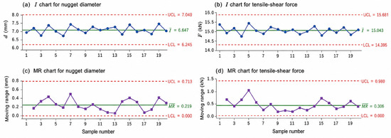
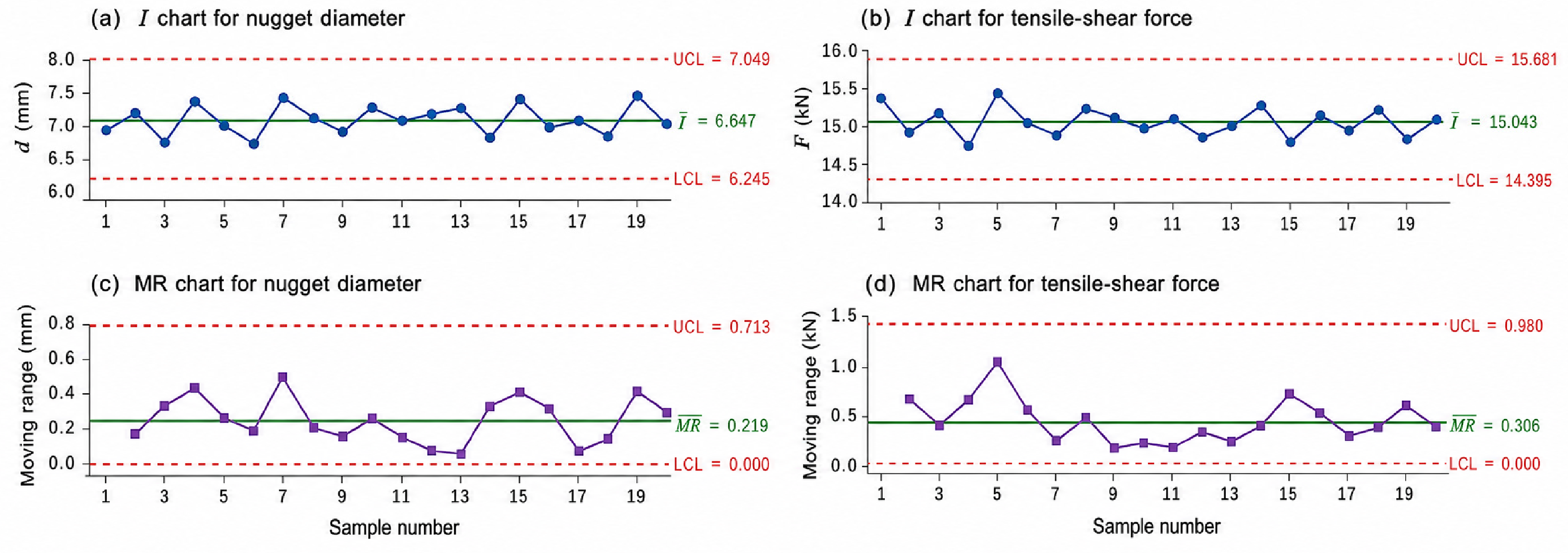
I-MR control charts were plotted from the 20 validation welds (Figure 8) and interpreted using ISO 7870-2:2023 run-pattern principles [34]. No point exceeds the control limits and no specified abnormal run pattern is observed. The I-chart control limits, calculated as x⁻ ± 2.66 MR⁻, are UCL = 7.09 mm and LCL = 5.92 mm for nugget diameter and UCL = 15.85 kN and LCL = 14.26 kN for tensile-shear force. Compared with measured Run 11 (6.77 ± 0.08 mm, CV = 1.18%, n = 3; 15.14 ± 0.30 kN, CV = 2.0%, n = 3), the selected compromise has a 4.0% smaller nugget diameter and higher diameter variability (CV = 2.10%), while tensile-shear force is 0.6% lower with lower variability (CV = 1.26%). Therefore, the selected condition is not globally superior. It is a variance-oriented compromise that improves tensile-shear stability at a small cost to nugget diameter and diameter stability.

Figure 8. Individual and moving range (I-MR) control charts for the validation tests: (a) I chart for nugget diameter (UCL = 7.09 mm, LCL = 5.92 mm); (b) I chart for tensile-shear force (UCL = 15.85 kN, LCL = 14.26 kN); (c) MR chart for nugget diameter; (d) MR chart for tensile-shear force.

4.6. Scope, Uncertainty, and Limitations

First, the repeated nominal condition differs significantly across the three independent single-factor batches (Table 3 note). Batch-to-batch offsets may reflect material lot variation, surface condition variation, environmental drift, and electrode condition. Electrode wear and dressing history were not quantitatively logged, so their contribution cannot be separated from other batch effects.

Second, Equation (6) is supported by the reported 20-run nugget diameter CCD, but it shows statistically significant lack of fit under the center-point pure-error test and is therefore used for local interpolation and trend interpretation. The significant lack-of-fit ($F_{\mathrm{LOF}}=11.28$, $p=0.009$; corrected from an earlier calculational error of F = 2.15, p = 0.18) relative to the center-point pure error suggests that unmodeled cubic curvature or interaction terms beyond the second order may exist in the nugget diameter response; future work should consider a Box-Behnken redesign with additional axial levels or a cubic RSM extension to resolve this residual structure. The complete 30-run tensile-shear CCD worksheet is unavailable. Equation (7) is therefore used only as an auxiliary local calibration, without the same validation status as the nugget diameter model. The n = 20 confirmation experiment verifies the selected operating point within the adopted error tolerance; it does not validate the full four-factor response surface or a global Pareto frontier.

Third, characterization was limited to optical microscopy, SEM morphology/fractography, and Vickers microhardness mapping. EBSD, EDS composition profiles, nanoindentation, thermal-cycle measurements, and electrode-wear metrology were not performed. Consequently, no Hall-Petch relationship, quantitative tempering-kinetic parameter, or coating diffusion coefficient is claimed.

Fourth, the HAZ descriptive screening envelope and specification limits are joint-, thickness-, material-, electrode-, and equipment-specific screening values. Broader generalization requires multi-batch electrode-life tests, additional validation points, thermal measurements, and product-specific acceptance criteria.

Fifth, only tensile-shear testing was performed; cross-tension, fatigue, and long-term electrode wear data are absent. These loading modes are critical for automotive body-in-white applications and should be addressed in future work.

Sixth, the Cpk assessment uses n = 20, which is below the n ≥ 30–50 typically recommended for stable capability estimation. The reported capability indices should be interpreted as exploratory short-term stability indicators rather than robust long-term process capability certification.

5. Conclusions

5.1. Main Conclusions

(1) Process-response trends: Single-factor experiments showed a Logistic-like increase and saturation of nugget diameter with current, a competitive effect of electrode force on nugget growth and HAZ softening, and an initial increase followed by deterioration with excessive welding time. The HAZ hardness response is quantified from Vickers microhardness maps.

(2) Within-batch factor ranking: In the orthogonal batch, electrode force contributed most to nugget-diameter variation (45.03%, F = 33.01, p < 0.01), whereas first-pulse current dominated tensile-shear force variation (51.73%, F = 139.50, p < 0.01). These rankings are within-batch variance decompositions and should not be pooled across the offset single-factor batches.

(3) Model scope and validation: The nugget-diameter CCD model has R² = 0.969 but shows significant lack of fit relative to the center-point pure error (FLOF = 11.28, p = 0.009); it is therefore treated as a local interpolation model. The tensile-shear Equation (7) is retained only as an auxiliary local calibration because its complete 30-run worksheet is unavailable and accordingly does not carry the same validation level as the nugget-diameter model. At the selected point, the nugget-diameter prediction differs from the measured mean by 1.01%, while the tensile-shear prediction is 4.39% below the measured mean; this validates the selected point only.

(4) Statistically informed decision result: The model-assisted compromise is 7.8 kA first-pulse current, 8.5 kA second-pulse current, 2.9 kN electrode force, and 13/17 cycles. The electrode force of 2.9 kN is slightly below the CCD stationary point (≈2.98 kN) and close to the screening optimum of 3.0 kN, balancing nugget growth against HAZ softening. Validation gave 6.51 ± 0.14 mm and 15.05 ± 0.19 kN (n = 20). Run 11 remains the measured performance-optimal orthogonal condition (6.77 ± 0.08 mm and 15.14 ± 0.30 kN); therefore, no global Pareto superiority is claimed for the compromise.

(5) Short-term stability: The validation sample has CVs of 2.10% for nugget diameter and 1.26% for tensile-shear force, and the I-MR charts show no out-of-control points or specified abnormal patterns. Capability indices are high under the study-specific alert limits, but they represent only an exploratory assessment of short-term statistical stability rather than evidence of industrial process capability or production certification.

(6) Joint-specific HAZ screening envelope: A joint-specific descriptive HAZ screening envelope (width < 0.7 mm; hardness loss < 50%) is proposed as a descriptive screening criterion for this 1.2 mm B1500HS/HC340/590DP joint and present equipment. The 0.7 mm threshold is a rounded engineering bound near the observed optimal-window HAZ response (Table 5: 0.67 ± 0.08 mm at 13/16 cycles), and the 50% limit derives from the Vickers microhardness profiles (Figure 4c: local minimum ~240 HV versus outer-region hardness ~460–510 HV at 3.0 kN); because this limit lies within the scatter of the data used to derive it, it is presented as a descriptive envelope without an explicit engineering margin. The envelope was never applied to the selected 13/17-cycle validation condition (Section 4.5) because HAZ width and microhardness were not measured on the n = 20 validation sample; it therefore remains conditional on the single-factor HAZ data in Section 3.2 and Section 3.3. It is a joint-specific engineering envelope requiring multi-batch and electrode-life validation, not an extension of ISO 10447 or ISO 14273.

5.2. Innovations

(1) A multi-scale quality-evaluation workflow was established by linking macroscopic nugget diameter and tensile-shear force with HAZ width and Vickers hardness loss, using only the microscopy, SEM morphology/fractography, and microhardness measurements available in this study.

(2) A sequential experimental strategy was implemented: orthogonal screening, nugget diameter CCD modeling, model-assisted decision analysis, and validation/SPC. This strategy distinguishes a supported local model from an auxiliary calibration and explicitly reports the unavailable raw tensile-shear CCD matrix as a limitation.

(3) The electrode force competition between nugget growth and HAZ softening is quantified through Holm contact-resistance scaling and a simplified bearing estimate, explaining the ANOVA contrast between a large force effect on diameter and a small effect on tensile-shear force without invoking fitted microstructure-property laws.

(4) A transparent decision framework distinguishes the measured performance-optimal condition (Run 11) from a validated variance-oriented compromise, avoiding unverified Pareto-optimality claims and explicitly reporting model-calibration limits.

(5) A joint-specific descriptive HAZ screening envelope (width < 0.7 mm; hardness loss < 50%) is proposed for the 1.2 mm B1500HS/HC340/590DP joint, with explicit dependence on equipment, thickness, and the observed single-factor HAZ response; it is a descriptive screening criterion and was not validated on the n = 20 confirmation sample, for which HAZ measurements were not taken.

(6) Batch-to-batch offsets are explicitly quantified and disclosed as a limitation, establishing a precedent for reproducibility discussion in RSW optimization studies and motivating future work on batch-effect mitigation strategies.

References

- Chen, W.; Zhu, Y.; Chen, L.; Chen, F.; Liu, B. Effects of Different Process Parameters on Mechanical Properties and Microstructures of Hot Stamping Boron Steel. Int. J. Adv. Manuf. Technol. 2021, 114, 939–948. [Google Scholar] [CrossRef] [Scilit]
- Capezza, C.; Centofanti, F.; Lepore, A.; Palumbo, B. Functional Clustering Methods for Resistance Spot Welding Process Data in the Automotive Industry. Appl. Stoch. Models Bus. Ind. 2021, 37, 908–925. [Google Scholar] [CrossRef] [Scilit]
- Soomro, I.A.; Pedapati, S.R.; Awang, M. A Review of Advances in Resistance Spot Welding of Automotive Sheet Steels: Emerging Methods to Improve Joint Mechanical Performance. Int. J. Adv. Manuf. Technol. 2022, 118, 1335–1366. [Google Scholar] [CrossRef] [Scilit]
- Holm, R.; Holm, E. Electric Contacts: Theory and Application, 4th ed.; Springer: Berlin/Heidelberg, Germany, 1967. [Google Scholar]
- Jia, X.; Wei, S.; Lu, S. Investigation on Microstructure and Tensile Shear Properties of 9Cr Oxide Dispersion Strengthened Steel Resistance Spot Welded Joint. Sci. Technol. Weld. Join. 2023, 28, 810–818. [Google Scholar] [CrossRef] [Scilit]
- Manladan, S.M.; Jang, Y.; Lee, Y.-K.; Park, Y.-D. Challenges and Advances in Resistance Spot Welding of Ultra-High Strength Hot-Stamped Steels: Coating Effect, Softening Phenomena, and Mechanical Performance. J. Mater. Res. Technol. 2024, 33, 7862–7887. [Google Scholar] [CrossRef] [Scilit]
- Zhou, X.; Wang, X.; Chen, Q.; Teng, F.; Cui, C.; Xiong, L.; Xing, Y.; Guo, W.; Sun, Q. Improving the Resistance Spot Welding Performance of Al-Si-Coated Press-Hardened 22MnB5 Steel through Preheating Treatment. Steel Res. Int. 2025, 96, 152–164. [Google Scholar] [CrossRef] [Scilit]
- Hıdıroğlu, M.; Kahraman, N. A Novel Approach for Improving Formation of Soft Zone in 22MnB5 and DP600 Materials by Resistance Spot Welding. Int. J. Adv. Manuf. Technol. 2025, 136, 2835–2856. [Google Scholar] [CrossRef] [Scilit]
- Nadimi, N.; Pouranvari, M. Understanding Interfacial Failure Mechanisms of Advanced High Strength Automotive Steels Resistance Spot Welds under Opening-Mode Loading. Eng. Fract. Mech. 2025, 313, 110627. [Google Scholar] [CrossRef] [Scilit]
- Stavropoulos, P.; Sabatakakis, K. Quality Assurance in Resistance Spot Welding: State of Practice, State of the Art, and Prospects. Metals 2024, 14, 185. [Google Scholar] [CrossRef] [Scilit]
- Feizollahi, V.; Bahmani, A.; Nadimi, N.; Salmani, M.R.; Pouranvari, M.; Park, Y.-D.; Ashiri, R. Factors Affecting Weld Quality in Resistance Spot Welding of Advanced High Strength Steels. Sci. Rep. 2025, 15, 30012. [Google Scholar] [CrossRef] [Scilit] [PubMed]
- Li, Z.X.; Wang, Y.Q.; Chen, Y.; Chen, F.; Yang, D.P.; Xie, G.M.; Yi, H.L. Critical Influence of FeAl and α-Fe Phases in Coating Layers on Resistance Spot Weldability of Al-Si Coated Press-Hardening Steels. J. Mater. Res. Technol. 2026, 41, 4015–4030. [Google Scholar] [CrossRef] [Scilit]
- ISO 10447:2022; Resistance Welding—Testing of Welds—Peel and Chisel Testing of Resistance Spot and Projection Welds. International Organization for Standardization: Geneva, Switzerland, 2022.
- ISO 14273:2016; Resistance Welding—Destructive Testing of Welds—Specimen Dimensions and Procedure for Tensile Shear Testing Resistance Spot, Seam and Embossed Projection Welds. International Organization for Standardization: Geneva, Switzerland, 2016.
- ISO 18278-2:2016; Resistance Welding—Weldability—Part 2: Evaluation Procedures for Weldability in Spot Welding. International Organization for Standardization: Geneva, Switzerland, 2016.
- Yuce, C. Multi-Objective Optimisation for Indentation Rate, Nugget Diameter and Tensile Load in Resistance Spot Welding Using Taguchi-Based Grey Relational Analysis. Int. J. Mater. Prod. Technol. 2021, 63, 321–338. [Google Scholar] [CrossRef] [Scilit]
- Boukraa, M.; Chekifi, T.; Lebaal, N. Friction Stir Welding of Aluminum Using a Multi-Objective Optimization Approach Based on Both Taguchi Method and Grey Relational Analysis. Exp. Tech. 2023, 47, 603–617. [Google Scholar] [CrossRef] [Scilit]
- Boulahem, K.; Salem, S.B.; Shiri, S.; Bessrour, J. Experimental Modeling and Multi-Response Optimization in Friction Stir Welding Process Parameters of AA2024-T3 Using Response Surface Methodology and Desirability Approach. Exp. Tech. 2024, 48, 833–849. [Google Scholar] [CrossRef] [Scilit]
- Rao, S.S.; Arora, K.S.; Sharma, L.; Chhibber, R. Modelling and Optimization of Resistance Spot Weld Responses Using RSM-GA Technique for DP590 Steel Sheets. Proc. Natl. Acad. Sci. India Sect. A Phys. Sci. 2022, 92, 453–466. [Google Scholar] [CrossRef] [Scilit]
- ISO 5821:2025; Resistance Welding—Spot Welding Electrodes—Female Electrode Caps. International Organization for Standardization: Geneva, Switzerland, 2025.
- Morales-Sánchez, G.; Collazo, A.; Doval-Gandoy, J.; Vázquez, A.; Álvarez, P. Influence of the Process Parameters on the Quality and Efficiency of the Resistance Spot Welding Process of Advanced High-Strength Complex-Phase Steels. Metals 2021, 11, 1545. [Google Scholar] [CrossRef] [Scilit]
- Kim, W.; Ji, C.-W. Trend of Resistance Spot Welding Technology of Al-Si Coated Hot-Stamped Boron Steel for Automobile Body. J. Weld. Join. 2022, 40, 187–197. [Google Scholar] [CrossRef] [Scilit]
- Okada, T.; Ueda, H.; Matsuda, K.; Miyazaki, Y.; Yasuyama, M.; Fujii, H. Effect of Strength of Steel Sheets on Tensile Shear Strength and Failure Mode of Dissimilar Joint of Spot Welds. Weld. Int. 2023, 37, 282–294. [Google Scholar] [CrossRef] [Scilit]
- Biele, L.; Schaaf, P.; Schmid, F. Method for Contact Resistance Determination of Copper during Fast Temperature Changes. J. Mater. Sci. 2021, 56, 3827–3845. [Google Scholar] [CrossRef] [Scilit]
- Tamizi, M.; Pouranvari, M.; Movahedi, M. The Role of HAZ Softening on Cross-Tension Mechanical Performance of Martensitic Advanced High Strength Steel Resistance Spot Welds. Metall. Mater. Trans. A 2021, 52, 655–667. [Google Scholar] [CrossRef] [Scilit]
- Ma, Y.; Takikawa, A.; Nakanishi, J.; Doira, K.; Shimizu, T.; Lu, Y.; Ma, N. Measurement of Local Material Properties and Failure Analysis of Resistance Spot Welds of Advanced High-Strength Steel Sheets. Mater. Des. 2021, 201, 109505. [Google Scholar] [CrossRef] [Scilit]
- Mohamadizadeh, A.; Biro, E.; Worswick, M. Failure Characterization and Meso-Scale Damage Modeling of Spot Welds in Hot-Stamped Automotive Steels Using a Hardness-Mapping Approach. Eng. Fract. Mech. 2022, 268, 108506. [Google Scholar] [CrossRef] [Scilit]
- Ribeiro, R.; Romão, E.L.; Luz, E.; Gomes, J.H.; Costa, S. Optimization of the Resistance Spot Welding Process of 22MnB5-Galvannealed Steel Using Response Surface Methodology and Global Criterion Method Based on Principal Components Analysis. Metals 2020, 10, 1338. [Google Scholar] [CrossRef] [Scilit]
- Zhu, R.; Yang, X.; Mi, Z.; Chen, J.; Li, Y. Constitutive Modeling for Elevated Temperature Flow Behavior of a Novel Cr-Si Alloyed Hot Stamping Steel. Mater. Res. Express 2023, 10, 066501. [Google Scholar] [CrossRef] [Scilit]
- Zhao, D.; Ivanov, M.; Wang, Y.; Liang, D.; Du, W. Multi-Objective Optimization of the Resistance Spot Welding Process Using a Hybrid Approach. J. Intell. Manuf. 2021, 32, 2219–2234. [Google Scholar] [CrossRef] [Scilit]
- Cao, X.; Li, Z.; Zhou, X.; Luo, Z.; Duan, J. Modeling and Optimization of Resistance Spot Welded Aluminum to Al-Si Coated Boron Steel Using Response Surface Methodology and Genetic Algorithm. Measurement 2021, 171, 108766. [Google Scholar] [CrossRef] [Scilit]
- Weng, H.; Jiang, J.; Feng, M.; Yao, M.; Chen, C.; Lian, G. Multi-Objective Optimizations of the Q355C Steel Gas Metal Arc Welding Process Based on the Grey Correlation Analysis. Int. J. Adv. Manuf. Technol. 2022, 121, 3567–3582. [Google Scholar] [CrossRef] [Scilit]
- Song, H.; Chen, X.; Zhang, S.; Xu, L. Multi-Objective Optimization Design of 6-UPS Parallel Mechanism Based on Taguchi Method and Entropy-Weighted Gray Relational Analysis. Appl. Sci. 2022, 12, 5836. [Google Scholar] [CrossRef] [Scilit]
- ISO 7870-2:2023; Control Charts—Part 2: Shewhart Control Charts. International Organization for Standardization: Geneva, Switzerland, 2023.
Disclaimer/Publisher’s Note: The statements, opinions and data contained in all publications are solely those of the individual author(s) and contributor(s) and not of MDPI and/or the editor(s). MDPI and/or the editor(s) disclaim responsibility for any injury to people or property resulting from any ideas, methods, instructions or products referred to in the content. |
© 2026 by the authors. Licensee MDPI, Basel, Switzerland. This article is an open access article distributed under the terms and conditions of the Creative Commons Attribution (CC BY) license.