Early Perception and Accurate Prediction of Hot Strip Flatness Based on Data Dimension Reduction and Multi-Output Regression

Abstract

To achieve early perception and accurate prediction of flatness quality, a partial least squares–particle swarm optimization–multi-output support vector regression (PLS-PSO-MSVR) is proposed. Firstly, we parameterized the flatness and used it as an evaluation indicator for flatness. Then, the prediction model was constructed using multi-output support vector regression (MSVR). In the modeling process, particle swarm optimization is used to optimize the parameters. To overcome the problem of information redundancy, reduce data dimensions to reduce computational time, and improve the prediction performance of the algorithm, this paper combines partial least squares and PSO-MSVR to achieve accurate prediction of the flatness features. Finally, the actual industrial process data from the hot rolling 1580 production line was used for validation, and the predicted performance was evaluated using mean absolute error (MAE), mean square error (MSE), root mean square error (RMSE), and coefficient of determination (R²). MAE decreased to 0.15, MSE decreased to 0.038, and RMSE decreased to 0.195. The R² approaches 1, indicating excellent model fit. This study achieves accurate prediction of the flatness characteristic coefficient, which not only enhances the diagnostic efficiency of steel flatness quality but also helps avoid unnecessary economic losses. Moreover, the prediction model provides a reliable basis for flatness control, offering operators a user-friendly reference tool. This approach compensates for the time lag inherent in the original system and contributes to improved accuracy in flatness control.

1. Introduction

Flatness, a critical quality attribute of hot-rolled strips, has become increasingly challenging to control in the face of growing personalized and customized market demands. Influenced by multiple factors—including raw material properties, equipment performance, and environmental conditions—issues like significant quality fluctuations within production batches and substantial variations between batches have become more prominent. The traditional flatness prediction mechanism model faces challenges including low accuracy, a long development cycle and slow calculation speed [1,2]. To improve the production quality and stability of the hot rolling process, a key aim of steel digitization is obviously to obtain effective information from massive production data, quickly predict the quality status of the strip, and analyze the abnormal production problems by means of data mining and data analysis [3,4].

In the process of shape quality diagnosis, a mathematical model of the rolling roll gap profile has been established to reveal the forming mechanism of flatness [5]. Yao established the global linear equations by decoupling, linearizing and discretizing the deformation model of the rolling process with the finite difference method [6]. On the basis of the above research, the metal flow model and the roll deformation model are combined. Through the combination of numerical simulation and experiment, Shin J.M. et al., considering the relationship between driving force, roll deflection, plate crown distribution and flatness, proposed a numerical model of flatness prediction based on the contact element method [7]. However, the combination of the strip plastic deformation model and the rolling mill roll elastic deformation model leads to instability in the iterative process of the prediction model, and even difficulty in convergence, due to the sensitivity of flatness and rolling force distribution to transverse thickness variations. To address this issue, Wang D.C. et al. adopted the inter-roll pressure distribution, rolling force distribution, and strip exit lateral displacement distribution as fundamental unknowns. By leveraging their intrinsic relationships, they integrated the strip plastic deformation model and the roll elastic deformation model into a unified system of linear equations, thereby avoiding iterative computations between the two models [8]. It is evident that various coupling models have been employed in flatness modeling. However, due to the complex rolling mechanisms and variable process constraints, mechanistic modeling incorporates numerous assumptions and empirical knowledge, making it difficult to ensure the accuracy of the flatness prediction and diagnostic process.

In recent years, the rapid development of intelligent algorithms, especially in the field of rolling, has made it possible to further improve the quality control of flatness [9]. With the collection and storage of a large amount of industrial data, data-based prediction and analysis of flatness quality has received widespread attention. In terms of data model-based prediction, algorithms such as artificial neural networks (ANN), convolutional neural networks (CNN), eXtreme Gradient Boosting (XGBoost) and back propagation neural network (BPNN) are widely used. Gao H pioneered the integration of a strip deviation measurement system with a time series prediction model to predict strip deviation and provide operators with timely warning signals [10]. The ANN model was used to predict the strip head deformation [11]. Ding J.G. et al. proposed the modeling concept of data and mechanism fusion, and constructed a CNN model for flatness control based on mechanism and data-driven fusion [12]. This model addresses the issue of low flatness control accuracy caused by insufficient parameter setting precision in factors such as rolling force and roll wear. Li M. et al. [13] proposed a method that combines XGBoost with the metallurgical mechanism to predict the mechanical properties of hot-rolled strip. In order to enhance the accuracy of flatness prediction, Shi K. et al. [14] developed a flatness quality prediction model based on BP neural network, using the flatness index as the quality indicator. To adapt to complex industrial environments and production demands, Liu J.Y. [15] proposed an improved Swish activation function based on batch normalization using a deep belief network to enhance the model’s prediction accuracy. Subsequently, algorithms such as sparrow search algorithm (SSA), particle swarm optimization (PSO), extreme learning machine (ELM) and deep multi-layer extreme learning machine (DELM) began to be applied to the flatness prediction model [16,17]. To enhance the preset and closed-loop feedback control performance for flatness, a prediction model based on class feature gradient improvement has been proposed [18]. However, this model requires a large amount of data for learning and training. Given the current small-scale customized production mode, it is difficult to obtain sufficient data volume and standard defect samples for effective model training. Therefore, prediction models that work with limited data are gaining attention, and Support Vector Regression (SVR) has become a mainstream prediction method [19,20]. Liu M.H. et al. [21] combined PSO, SVR, and BP neural networks to predict strip crown.

In addition, the complex production process of strip steel leads to numerous issues with production data, including redundancy, high dimensionality, and coupling. High-dimensional data results in problems such as slow training speed and low model accuracy. To enhance the training efficiency of prediction models, it is effective to reduce data dimensionality and improve data quality by extracting meaningful information and enhancing the signal-to-noise ratio of the original data. Commonly used feature extraction methods include principal component analysis (PCA), independent component analysis (ICA), and partial least squares regression (PLS) [22,23,24]. Wang Z.H. et al. [25] proposed a novel hybrid model for predicting strip profile and flatness by combining the extreme learning machine (ELM) with industrial data. This model uses PCA to reduce the dimensionality of input data from modeling samples, thereby improving training speed. Ji Y.F. et al. [26] developed a support vector machine (SVM) prediction model optimized by PCA and the cuckoo search (CS) algorithm, achieving better prediction accuracy and convergence speed. Song L.B. et al. [27] introduced a machine learning-based method for predicting and diagnosing the convexity of hot-rolled strip, applying PCA to analyze causes of abnormal fluctuations in convexity. By evaluating the degree of influence of variables on quality, they performed feature extraction on process information, effectively improving model efficiency. However, under the above feature extraction conditions, the constraining effect of quality indicators on process variables was not taken into account, which compromised the integrity of the model training data. However, in the process of predicting the flatness of hot-rolled strips, it has been observed that flatness encompasses various fundamental flatness modes. To monitor and diagnose shape variations, this study parameterizes the strip shape using coefficients of different orders to characterize its fluctuations. Due to the high correlation among the coefficients of various orders, it is clearly unreasonable for the aforementioned prediction methods to treat multidimensional outputs as separate and independent problems. Therefore, this paper focuses on the flatness prediction problem with multidimensional feature outputs. In light of this, the study investigates a method based on PLS feature extraction and MSVR to achieve accurate prediction of strip shape characteristics.

The main contributions of this paper are as follows: A new flatness quality feature prediction model based on feature extraction and optimized MSVR was proposed to accurately predict the flatness quality under multiple feature parameters and reveal the changes in flatness characteristics. The relevant data of flatness of the 1580 hot rolling production line were collected for verification. And mean absolute error [28] (MAE), mean square error (MSE), root mean square error (RMSE) and determination coefficient R2 are introduced to evaluate the predictive performance of different models. The structure of this paper is organized as follows: Section 2—the parameterized characterization methods of the flatness characteristics of hot-rolled strip are introduced as the output for predicting the flatness characteristics. Section 3—the multi-output MSVR model is introduced, and the PSO algorithm is introduced to optimize the model parameters. Section 4—the model is validated and discussed through on-site actual production data. Section 5 summarizes the conclusion. In contrast to existing approaches, the proposed PLS-PSO-MSVR model offers three specific advantages. First, unlike single-output prediction models (e.g., standard SVR, BPNN, XGBoost) that treat each flatness characteristic coefficient independently, our method explicitly models the inherent correlations among multiple flatness outputs ($c_1$–$c_4$ and PLA (the standard deviation of flatness)) using a multi-output support vector regression framework. Second, while previous studies have employed PCA for dimensionality reduction in strip flatness prediction, PCA ignores the relationship between process variables and quality indicators. Our use of PLS preserves the covariance structure between inputs and outputs, which is particularly beneficial when flatness characteristics are strongly coupled with rolling parameters. Third, compared to traditional empirical parameter selection for SVR-based models, PSO provides a systematic and efficient way to determine kernel parameters and penalty factors, avoiding blind trial-and-error and improving generalization performance.

2. Methods

2.1. MSVR Prediction Model

MSVR is an extension of the SVR model that adapts to multi-objective output systems [29]. The method is suitable for solving the multi-dimensional output problem of prediction of multiple characteristics of a hot-rolled shape. In this study, the actual production data of 1580 stainless steel production process is used as input to predict the flatness characteristic parameters of the hot rolling production line.

$$Q={\left\{\left({\mathit{x}}_1,{\mathit{y}}_1\right),\left({\mathit{x}}_2,{\mathit{y}}_2\right),\cdots ,\left({\mathit{x}}_l,{\mathit{y}}_l\right)\left|{\mathit{x}}_i\in {\mathit{R}}^m,\right.{\mathit{y}}_i\in {\mathit{R}}^n\right\}}^N$$

(1)

where ${\mathit{x}}_i$ and ${\mathit{y}}_{\mathrm{i}}$ represent process variables and quality variables, respectively. n and m are dimensions of input and output variables, respectively. N represents the total sample size. Establish a multi-objective regression model based on input and output data.

$$f_j\left(\mathit{x},{\mathit{\omega }}_j,b_j\right)=⟨{\mathit{\omega }}_j,\mathit{x}⟩+b_j$$

(2)

where $b_j\in \mathit{R}$, $⟨,⟩$ is the dot product, ${\omega }_j=\left[{\omega }_{j1}\cdots {\omega }_{jn}\right]$, $j=1,\cdots ,m$.

$$y_i=f\left(x_i\right)=\mathit{W}\bullet \phi \left({\mathit{x}}_i\right)+\mathit{B}$$

(3)

where $\mathit{W}={\left[{\mathsf{\omega }}_1\cdots {\mathsf{\omega }}_{\mathrm{m}}\right]}^{\mathrm{T}}$ is a matrix composed of weight vectors, and $\mathit{B}={\left[b_1\cdots b_m\right]}^T$ is a vector composed of real numbers.

As can be seen from the above, to solve the multi-objective regression problem, it is necessary to solve the output of each objective regression ${\omega }_j$ and $b_j\left(j=1,\cdots ,m\right)$. Therefore, the quadratic programming problem is solved according to the $\mathrm{V}\mathrm{a}\mathrm{p}\mathrm{n}\mathrm{i}\mathrm{k}$ structural risk minimization principle and the output error minimization principle.

$$\min {\displaystyle {\displaystyle \sum _{j=1}^m}{‖{\omega }_j‖}^2}+C{\displaystyle {\displaystyle \sum _{i=1}^m}{\xi }_i^2}$$

(4)

$$s.t.\left\{\begin{array}{c}‖y_i-f\left(x_i\right)‖\le \epsilon +{\xi }_i\\ {\xi }_i\ge 0\end{array}\right.$$

(5)

where ${\xi }_i$ represents the relaxation variable of $x_i$, $\mathrm{C}$ represents the penalty factor, $\epsilon$ represents the parameter of the loss function.

From the constraints of equations, the highest degree of the polynomial for solving process constraints is not 1, and this function cannot be solved as an affine function. Therefore, the dual space method cannot be used to solve the quadratic programming problem. In this study, the output prediction of a multivariable is realized by hyperparameter optimization, and the loss function $L_s\left(·\right)$ is redefined on the hypersphere, and the one-dimensional $\epsilon$ insensitive loss function is expanded to be multidimensional.

$$L_{\epsilon }\left(u_i\right)=\left\{\begin{array}{l}0, u_i<\epsilon \\ {\left(u_i-\epsilon \right)}^2,u_i\ge \epsilon \end{array}\right.$$

(6)

$$u_i=‖e_i‖=\sqrt{e_i^{\mathrm{T}}{e}_i}$$

(7)

$$e_i^{\mathrm{T}}=y_i^{\mathrm{T}}-\mathit{W}{\phi }^{\mathrm{T}}\left({\mathit{x}}_i\right)-{\mathit{{\rm B}}}^{\mathrm{T}}$$

(8)

Based on the above process, the following objective function is obtained.

$$\min L_{\epsilon }\left(\mathit{W},\mathit{B}\right)={\displaystyle \frac{1}{2}}{\displaystyle {\displaystyle \sum _{j=1}^m}{‖{\omega }_j‖}^2}+C{\displaystyle {\displaystyle \sum _{i=1}^N}{‖u_i‖}^2}$$

(9)

The iterative weighted least square method is used to solve the problem. In the above optimization objective function, the first order Taylor series expansion is used to approximate the loss function.

$$L_{\epsilon }^{\prime }\left(\mathit{W},\mathit{B}\right)={\displaystyle \frac{1}{2}}{\displaystyle \sum _{j=1}^m{‖{\omega }_j‖}^2}+C\left({\displaystyle \sum _{i=1}^{N}L(u_i^k)}+{\left.{\displaystyle \frac{\mathrm{d}L(u_i)}{\mathrm{d}{u}_i}}\right|}_{u_i^k}{\displaystyle \frac{{\left(e_i^k\right)}^{\mathrm{T}}}{u_i^k}}\left(e_i-e_i^k\right)\right)$$

(10)

where $k$ represents the number of iteration cycles. Construct the quadratic approximation of the above equation.

$$\begin{array}{l}{L}_{\epsilon }^{″}\left(\mathit{W},\mathit{B}\right)={\displaystyle \frac{1}{2}}{\displaystyle \sum _{j=1}^m{‖{\omega }_j‖}^2}+C\left({\displaystyle \sum _{i=1}^{N}L(u_i^k)}+{\left.{\displaystyle \frac{\mathrm{d}L(u_i)}{\mathrm{d}{u}_i}}\right|}_{u_i^k}{\displaystyle \frac{u_i^2-{\left(u_i^k\right)}^2}{2u_i^k}}\right)\\ ={\displaystyle \frac{1}{2}}{\displaystyle {\displaystyle \sum _{j=1}^m}{‖{\omega }_j‖}^2}+{\displaystyle \frac{1}{2}}{\displaystyle {\displaystyle \sum _{j=1}^N}{a}_i{u}_i^2}+CT\end{array}$$

(11)

$$a_i={\displaystyle \frac{C}{u_i^k}}{\left.{\displaystyle \frac{\mathrm{d}L\left(u_i\right)}{\mathrm{d}{u}_i}}\right|}_{u_i^k}=\left\{\begin{array}{c} 0 , u_i^k<\epsilon \\ {\displaystyle \frac{2C\left(u_i^k-\epsilon \right)}{u_i^k}}, u_i^k\ge \epsilon \end{array}\right.$$

(12)

where $CT$ is a constant term that does not depend on $\mathit{W}$ and $\mathit{B}$.

$\mathit{W}$ and $\mathit{B}$ are decoupled, and the partial derivative of $\mathit{W}$ and $\mathit{B}$ can be directly calculated to be zero, thus obtaining an approximate solution for $\mathit{W}$ and $\mathit{B}$. Therefore, calculate the $\mathit{W}$ and $\mathit{B}$ that minimize the overall loss of the sample set, and complete the MSVR prediction model.

The algorithm process is shown in Table 1.

Table 1. Algorithm optimization solution process.

$\mathbf{M}\mathbf{S}\mathbf{V}\mathbf{R}$ Solving Process
Step 1	Parameter initialization: $k=0,$${\mathit{W}}_k=0,$${\mathit{B}}_k=0.$ Calculate $u_i^k$ and $a_i.$
Step 2	Solve the value of the quadratic approximation function, denoted as ${\mathit{W}}_s$ and ${\mathit{B}}_s.$ Define descent direction: $P_k=\left[\begin{array}{c}{\mathit{W}}_s-{\mathit{W}}_k\\ {\left({\mathit{B}}_s-{\mathit{B}}_k\right)}^T\end{array}\right].$
Step 3	Calculate the next iteration solution: $\left[\begin{array}{c}{\mathit{W}}_{k+1}\\ {\left({\mathit{B}}_{k+1}\right)}^T\end{array}\right]=\left[\begin{array}{c}{\mathit{W}}_k\\ {\left({\mathit{B}}_k\right)}^T\end{array}\right]+{\eta }_k{\mathit{P}}_k.$ Backtracking method for calculating iteration step size ${\eta }_k.$
Step 4	Calculate $u_i^{k+1}$ and $a_{\mathrm{i}}.$ Let $k=k+1,$ determine $L_s\left({\mathit{W}}_{k+1},{\mathit{B}}_{k+1}\right)<L_s\left({\mathit{W}}_k,{\mathit{B}}_k\right).$ Otherwise, return to Step 2 until convergence.

To obtain ${\mathit{W}}_s$ and ${\mathit{B}}_s$, by solving for each component with the gradient of equation equal to zero, we can obtain:

$${\nabla }_{{\omega }_j}{L}_{\mathsf{\epsilon }}^{″}={\mathit{\omega }}_j-{\displaystyle \sum _i\mathit{\phi }\left(x_i\right)a_i}\left(y_{ij}-{\mathit{\phi }}^T\left(x_i\right){\mathit{\omega }}_j-{\mathit{b}}_j\right)=0$$

(13)

$${\nabla }_{b_j}{L}_{\mathsf{\epsilon }}^{″}=-{\displaystyle \sum _i{a}_i}\left(y_{ij}-{\mathit{\phi }}^T\left(x_i\right){\mathit{\omega }}_j-{\mathit{b}}_j\right)=0$$

(14)

The above equation is expressed in linear form as:

$$\left[\begin{array}{cc}{\mathit{\phi }}^{\mathrm{T}}{\mathit{D}}_a\mathit{\phi }+\mathit{I}& \mathit{\phi }\mathit{a}\\ {\mathit{a}}^{\mathrm{T}}\mathit{\phi }& {\mathit{I}}^{\mathrm{T}}\mathit{a}\end{array}\right]\left[\begin{array}{c}{\mathit{\omega }}_j\\ {\mathit{b}}_j\end{array}\right]=\left[\begin{array}{c}{\mathit{\phi }}^{\mathrm{T}}{\mathit{D}}_a{\mathit{y}}_j\\ {\mathit{a}}^{\mathrm{T}}{\mathit{y}}_j\end{array}\right]$$

(15)

where $\mathit{\phi }={\left[\mathit{\phi }\left(x_1\right),\cdots ,\mathit{\phi }\left(x_N\right)\right]}^T$, ${\mathit{D}}_a=diag\left(a_1,\cdots ,a_N\right)$, $\mathit{a}={\left[a_1,\cdots ,a_N\right]}^T$, ${\mathit{y}}_j=\left[y_{j1},\cdots ,y_{jN}\right]$, $j=1,\cdots ,m$ is the $j$-th component of the multidimensional output model. $\mathit{I}={\left[1,\cdots ,1\right]}^{\mathrm{T}}$ is a column vector with all 1.

Through the Presenter theorem [29], under general conditions, the optimal solution of a learning problem can be represented in a high-dimensional feature space using a linear combination of training features:

$${\mathit{\omega }}_j={\displaystyle {\sum }_i\mathit{\phi }\left(x_i\right)}{\mathit{\beta }}_j={\mathit{\phi }}^{\mathrm{T}}{\mathit{\beta }}_j$$

(16)

$$\left[\begin{array}{cc}{\mathit{D}}_a^{-1}+\mathit{K}& \mathit{I}\\ {\mathit{a}}^{\mathrm{T}}\mathit{K}& {\mathit{I}}^{\mathrm{T}}\mathit{a}\end{array}\right]\left[\begin{array}{c}{\mathit{\beta }}_j\\ {\mathit{b}}_j\end{array}\right]=\left[\begin{array}{c}{\mathit{y}}_j\\ {\mathit{a}}^{\mathrm{T}}{\mathit{y}}_j\end{array}\right]$$

(17)

where $\mathit{K}$ represents the kernel matrix, and in this paper, the Gaussian radial basis kernel function is selected. This function can effectively solve the nonlinear relationship between process and quality, and is superior to other kernel functions in modeling and root mean square error. Its expression form is as follows:

$$K=\varphi \left(\mathit{x}\right)\varphi \left(\mathit{x}\prime \right)=\exp (-{\displaystyle \frac{{‖x-x\prime ‖}^2}{2{\delta }^2}})$$

(18)

where $x$ represents the sample data point, $x^{\prime }$ represents the center point of the kernel function, and $\delta$ represents the width coefficient of the kernel function, respectively.

2.2. Optimization of Flatness Feature Prediction Model for MSVR

The standard MSVR model, using default parameter settings (penalty factor C = 1, RBF kernel parameter δ = 1), serves as a non-optimized baseline. It is included solely to illustrate the limitations of empirical parameter selection and to justify the need for systematic optimization using PSO. The MSVR prediction model uses kernel functions to map low-dimensional feature space vectors to a high-dimensional feature space to enhance the interpretability of nonlinear relationships between variables. However, the key parameters of the model—the kernel parameter δ and the penalty factor C—are difficult to guarantee optimal performance if selected empirically. Therefore, systematic optimization of these parameters is necessary. Assuming that the cluster is composed of $N$ particles, and the dimensions and velocities of each particle are $d$-dimensional vectors, the position of the $i$-th particle in $d$-dimensional space is:

$$x_i=\left[x_{i1},x_{i2},x_{i3},\cdots ,x_{id}\right]\left(i=1,2,\cdots ,N\right)$$

(19)

The speed is:

$$v_i=\left[v_{i1},v_{i2},v_{i3},\cdots ,v_{id}\right]\left(i=1,2,\cdots ,N\right)$$

(20)

Each particle is randomly distributed in the $d$-dimensional space and tracks individual extremum. The optimal position experienced by the $i$-th particle during the iteration process is local optimal, as shown in the following equation:

$$p_i=\left[p_{i1},p_{i2},p_{i3},\cdots ,p_{id}\right]\left(i=1,2,\cdots ,N\right)$$

(21)

The optimal position experienced by the entire population during the search process is the global optimal, as shown in the following equation:

$$p_m=\left[p_{m1},p_{m2},p_{m3},\cdots ,p_{md}\right]\left(m=1,2,\cdots ,N\right)$$

(22)

In the optimization process, the fitness value is recalculated every time the particle position and velocity are updated. By comparing the fitness value of each particle, the better fitness value is assigned to the individual extreme value and the population extreme value; until the iteration number condition is reached, the optimal population position is output [30]. The PSO iteration process updates the particle state as follows:

$$v_i^{t+1}=\zeta v_i^t+{\phi }_1{\beta }_1\left(p_i^t-x_i^t\right)+{\phi }_2{\beta }_2\left(p_m^t-x_i^t\right)$$

(23)

$$x_i^{t+1}=x_i^t+v_i^t$$

(24)

where ${\phi }_1,{\phi }_2$ represent the non-negative learning factor, taken as ${\phi }_1={\phi }_2=2$. ${\beta }_1,{\beta }_2$ are a random number, ${\beta }_1,{\beta }_2\in \left[\mathrm{0,1}\right]$. $\mathsf{\zeta }$ is the inertia factor, which is a constant value. $t$ is the number of iterations, $t=\mathrm{1,2},\cdots ,T$. T represent the maximum number of iterations.

To improve the prediction accuracy of the model, the MSVR parameters are optimized based on the above PSO algorithm, and the fitness values of each particle are calculated. The root mean square error (MSE) is used as the fitness function:

$$\mathrm{M}\mathrm{SE}={\displaystyle \frac{1}{l}}{\displaystyle \sum _{i=1}^l{\left(f(x_i)-y_i\right)}^2}$$

(25)

where $f\left(x_i\right)$ represents the predicted value of the test data, $y_i$ represents the actual value of the test data, and $l$ represents the number of samples.

Therefore, the PSO algorithm optimization process is shown in Table 2.

Table 2. PSO Algorithm Process.

PSO Algorithm Process:
Step 1	Initialize PSO parameters.
Step 2	Calculate the fitness value of each particle.
Step 3	Comparing the value of particle fitness function, the local and global optimal values are obtained.
Step 4	Update particle velocity and position.
Step 5	Determine the iteration number condition, and if the condition is met, output the optimal solution. If not satisfied, return to Step 2.
Step 6	Obtain optimization parameters.

2.3. Feature Extraction Based on PLS

To reduce the data dimension, reduce the calculation time and improve the prediction performance of the algorithm. In this study, a shape feature prediction model coupled with PLS and MSVR is proposed to solve the problem of data redundancy and improve the prediction accuracy of quality features. Assume there are $p$ independent variables and $q$ dependent variables to form a data matrix ${\mathit{X}}_{n\times p}$ and ${\mathit{Y}}_{n\times q}$.

Determine the number of principal components $h$ using the cross-validation method [31]. Define its cross validity:

$$PRES{S}_h={\displaystyle \frac{1}{m_t}}\sqrt{{\displaystyle \sum _{i=1}^{m_t}{\left({\widehat{y}}_i-y_i\right)}^2}}$$

(26)

$$Q_h^2=1-{\displaystyle \frac{PRES{S}_h}{S{S}_{h-1}}}$$

(27)

where ${PRESS}_h$ represents the total prediction error, $m_t$ represents the number of predicted validation data samples, ${\widehat{y}}_i$ represents the predicted value, $y_i$ represents the predicted validation data. According to the above cross-validation, when $Q_h^2\ge 0.0975$, the first $h$ components are taken, otherwise, the last newly added principal component can be discarded. Use the extracted principal components to construct training samples $\left\{\left({\mathit{t}}_i,y_i\right),i=\mathrm{1,2},\cdots ,h\right\}$ as input for the PLS-PSO-MSVR flatness feature prediction model.

2.4. Implementation of PLS-PSO-MSVR

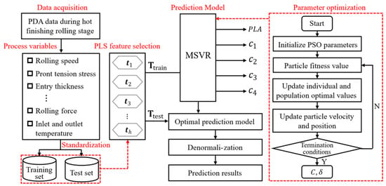
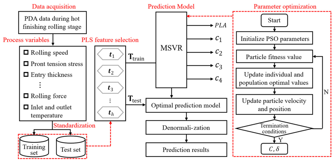
The flow chart of the $\mathrm{P}\mathrm{L}\mathrm{S}$-$\mathrm{P}\mathrm{S}\mathrm{O}$-$\mathrm{M}\mathrm{S}\mathrm{V}\mathrm{R}$ method is shown in Figure 1.

Figure 1. PLS-PSO-MSVR procedure.

The implementation process is mainly divided into the following steps:

Step 1: Collect the process data and flatness data of 1580 finishing the rolling stage, namely the training and testing data of the model.

Step 2: Remove the outlier from the original data and standardize the data.

Step 3: Divide the standardized dataset into training and testing sets.

Step 4: Parameterize the flatness data and extract the flatness feature coefficients and $\mathrm{P}\mathrm{L}\mathrm{A}$ as the model output.

Step 5: Extract the latent variable score matrix ${\mathrm{T}}_{\mathrm{t}\mathrm{r}\mathrm{a}\mathrm{i}\mathrm{n}}$ from the training set to construct the $\mathrm{M}\mathrm{S}\mathrm{V}\mathrm{R}$ framework. At the same time, the potential test set variable score matrix ${\mathrm{T}}_{\mathrm{t}\mathrm{e}\mathrm{s}\mathrm{t}}$ is used to verify the accuracy of the model.

Step 6: Use PSO to evaluate $\mathrm{R}\mathrm{B}\mathrm{F}$ kernel parameters $\mathsf{\delta }$ and penalty factor $\mathrm{C}$ for optimization. Obtain optimal prediction results.

Step 7: The prediction performance of $\mathrm{P}\mathrm{L}\mathrm{S}$-$\mathrm{P}\mathrm{S}\mathrm{O}$-$\mathrm{M}\mathrm{S}\mathrm{V}\mathrm{R}$ and other comparison models is evaluated by MAE, MSE, RMSE and ${\mathrm{R}}^2$, which are defined as follows:

$$E_{\mathrm{MAE}}={\displaystyle \frac{1}{N}}{\displaystyle \sum _{i=1}^N\left|Y_i-{\widehat{Y}}_i\right|}$$

(28)

$$E_{\mathrm{MSE}}={\displaystyle \frac{1}{N}}{\displaystyle \sum _{i=1}^N{\left(Y_i-{\widehat{Y}}_i\right)}^2}$$

(29)

$$E_{\mathrm{RMSE}}=\sqrt{{\displaystyle \frac{{\displaystyle \sum _{i=1}^N{\left(Y_i-{\widehat{Y}}_i\right)}^2}}{N}}}$$

(30)

$$R^2=1-{\displaystyle \frac{{\displaystyle \sum _{i=1}^N{‖Y_i-{\widehat{Y}}_i‖}^2}}{{\displaystyle \sum _{i=1}^N{\left(Y_i-\overline{Y}\right)}^2}}}$$

(31)

where $Y_i$ and ${\widehat{Y}}_i$ represent the true value and the predicted value, respectively. $\overline{Y}$ represents the average of the measured values. $N$ represents the number of samples.

3. Parameterized Characterization of the Flatness Characteristics of Hot-Rolled Strip

3.1. Flatness Parameterization Based on Legendre Polynomial

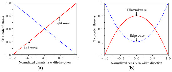
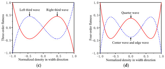
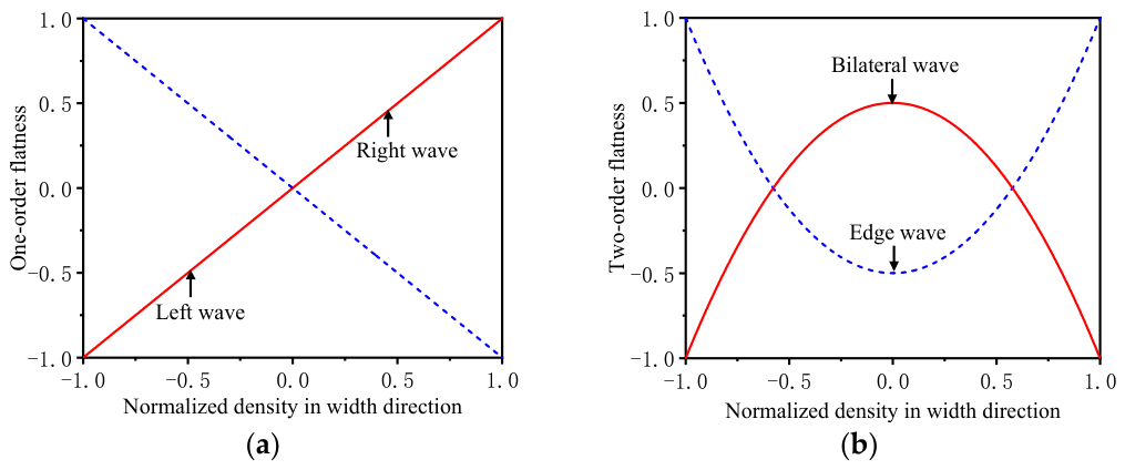
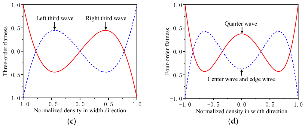
Selecting the flatness pattern recognition model as the indicator feature for parameterization of flatness quality, analyzing and identifying the types of flatness defects in the measured flatness signals, providing a basis for parameterization of flatness recognition. Based on the process and control technology of the rolling mill, as well as the characteristics of plate shape defects in the 1580 hot rolling production line of a certain steel, Legendre orthogonal polynomials $\left\{Y_1\left(x\right),Y_2\left(x\right),Y_3\left(x\right),Y_4\left(x\right)\right\}$ of degree 1,2,3,4 are selected to represent the benchmark mode of the plate shape, where $x$ is the position of the standardized flatness measurement point. The Legendre polynomial of each order is used to parametrically represent the flatness, and they are used as the benchmark mode of the flatness parameterization process, as shown in Figure 2.

Figure 2. Flatness reference mode represented by Legendre polynomials. (a) One-order flatness; (b) Two-order flatness; (c) Three-order flatness; (d) Four-order flatness.

The flatness distribution across the strip width is represented by a linear combination of Legendre polynomials. The coefficient $c_1$ represents the first-order (linear) component, corresponding to left–right asymmetry (e.g., edge wave on one side only). The second-order coefficient $c_2$ describes a symmetric parabolic shape, typically associated with center buckle (positive $c_2$) or edge wave (negative $c_2$). The third-order coefficient $c_3$ reflects a more complex “W-shaped” or inverse-W asymmetry, while $c_4$ captures higher-order oscillations such as quarter buckles. The parameter PLA (predicted length adjustment) represents the overall deviation of the strip from a perfectly flat state, often used as a comprehensive flatness index.

Parameterize the flatness of rolled plates using Legendre polynomials, as shown in the following equation:

$$\sigma \left(x\right)=c_1{Y}_1\left(x\right)+c_2{Y}_2\left(x\right)+c_3{Y}_4\left(x\right)+c_4{Y}_4\left(x\right)$$

(32)

where $\sigma \left(x\right)$ represents the flatness value along the width direction of the strip, $c_k$ is the flatness characteristic parameter, $k=\mathrm{1,2},\mathrm{3,4}$. Given the flatness data point $\left(x_i,{\sigma }_i\right)(i=\mathrm{1,2},\cdots ,m)$, establish a flatness pattern recognition model based on the least squares method, so that the fitted flatness value function $Y\left(x_i\right)$ satisfies $\mathrm{m}\mathrm{i}\mathrm{n}{\displaystyle {\sum }_{i=1}^m}{\left[Y\left(x_i\right)-{\sigma }_i\right]}^2$. Turning to the extremum problem:

$$\varphi =\left(c_1,c_2,c_3,c_4\right)={\displaystyle \sum _{i=1}^m{\left[{\displaystyle \sum _{j=1}^4{c}_j{Y}_j\left(x_i\right)-{\sigma }_i}\right]}^2}$$

(33)

where $x_i$ represent the position of the measuring point along the board width direction, and ${\sigma }_i$ is the flatness value at point $x_i$, $i=\mathrm{1,2},\cdots ,9$.

Construct a matrix of flatness measurement values.

$$\mathit{\sigma }={\left[{\sigma }_1,{\sigma }_2,\cdots ,{\sigma }_9\right]}^{\mathrm{T}}$$

(34)

Based on Legendre polynomials as orthogonal polynomials, the matrix $\mathit{P}$ is composed of Legendre polynomials.

$$\mathit{P}=\left[Y_1^{\mathrm{T}}\left(x\right),Y_2^{\mathrm{T}}\left(x\right),Y_3^{\mathrm{T}}\left(x\right),Y_4^{\mathrm{T}}\left(x\right)\right]=\left[\begin{array}{ccc}{Y}_{11}& \cdots & Y_{41}\\ ⋮& ⋮& ⋮\\ Y_{1n}& \cdots & Y_{4n}\end{array}\right]$$

(35)

where $Y_{ij}=Y_i\left(x_j\right)\left(i=\mathrm{1,2},\mathrm{3,4};j=\mathrm{1,2},\cdots ,n\right)$, $x_j$ represents the coordinate value of the $j$-th sampling point along the width direction of the strip. Obtain the flatness characteristic coefficient $\mathit{c}$.

$$\mathit{c}={\left[c_1,c_2,c_3,c_4\right]}^{\mathrm{T}}={\mathit{P}}^T\mathit{\sigma }$$

(36)

The flatness after rolling is composed of the above-mentioned flatness base mode, and the flatness quality is quantitatively represented by using the flatness characteristic parameter $c_k$. According to the Legendre polynomial characterization characteristics of flatness quality, if there is no abnormal fluctuation in the flatness quality, the characteristic parameters of each order of the flatness will not show obvious statistical characteristics. When the flatness is abnormal, a certain order coefficient will appear significantly prominent.

3.2. Flatness Parameterization Based on PLA

To achieve rapid diagnosis of flatness quality and rapid evaluation of strip quality, the detection data from nine channels of the flatness tester are converted into one-dimensional flatness standard deviation data [32,33], thereby achieving evaluation of the overall state of the flatness. The data conversion is as follows:

$$PLA=\sqrt{{\displaystyle \frac{{\displaystyle \sum _{i=1}^m\Delta y_i^2}}{m-1}}}$$

(37)

where $m$ represents the number of flatness detection channels, $∆y_i$ represents the straightness deviation of the measurement channel, and $PLA$ represents the standard deviation of flatness.

The above formula is used to achieve one-dimensional conversion of multi-channel data on flatness, and the overall situation of flatness fluctuation during the rolling process is judged through $PLA$.

4. Validated in the Measured Data

4.1. Flatness-Related Data Acquisition

The data related to strip quality comes from offline PDA (Process Data Acquisition System) data of a 1580 mm hot-rolled strip production line, which was put into operation in 2008. The product specifications are $1.2~12.7 \mathrm{mm}\times 800~1400 \mathrm{mm}$. Use the IBA Analyzer software v8.3.1 to read data and extract the required data. In the data file, each file includes all production data of a coil of strip. Based on the strip production data, the data set is divided after preprocessing, and the data set division structure is in accordance with the ratio of 2:1. Based on the production data file, the relevant data of plate shape is extracted as shown in Table 3. This includes 45 process variables and one quality variable, namely the flatness of the strip. This article parameterizes the flatness and converts it into the flatness feature parameter $PLA$, $c_1$, $c_2$, $c_3$, $c_4$ as output. At the beginning of the modeling process, preprocess the original sample data. In this study, the Pauta criterion in statistical hypothesis-testing was used to process and remove abnormal data. Then standardize the data.

Table 3. Flatness-related parameters.

Variable Category	Variable	Unit	F1	F2	F3	F4	F5	F6	F7
Process variables	Rolling speed	m/s	√	√	√	√	√	√	√
	Front tension stress	MPa	√	√	√	√	√	√	-
	Entry thickness	mm	√	√	√	√	√	√	√
	Rolling force	MN	√	√	√	√	√	√	√
	Roll gap value	mm	√	√	√	√	√	√	√
	Bending roll force	kN	√	√	√	√	√	√	√
	Finish rolling inlet temperature	°C	√	-	-	-	-	-	-
	Finish rolling outlet temperature	°C	-	-	-	-	-	-	√
	Finish-rolled outlet thickness	mm	-	-	-	-	-	-	√
	Finish rolling outlet width	mm	-	-	-	-	-	-	√
Quality variables	Flatness	I	-	-	-	-	-	-	√

4.2. Prediction Result

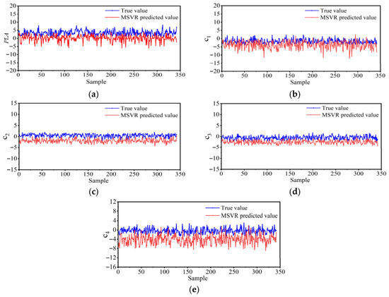
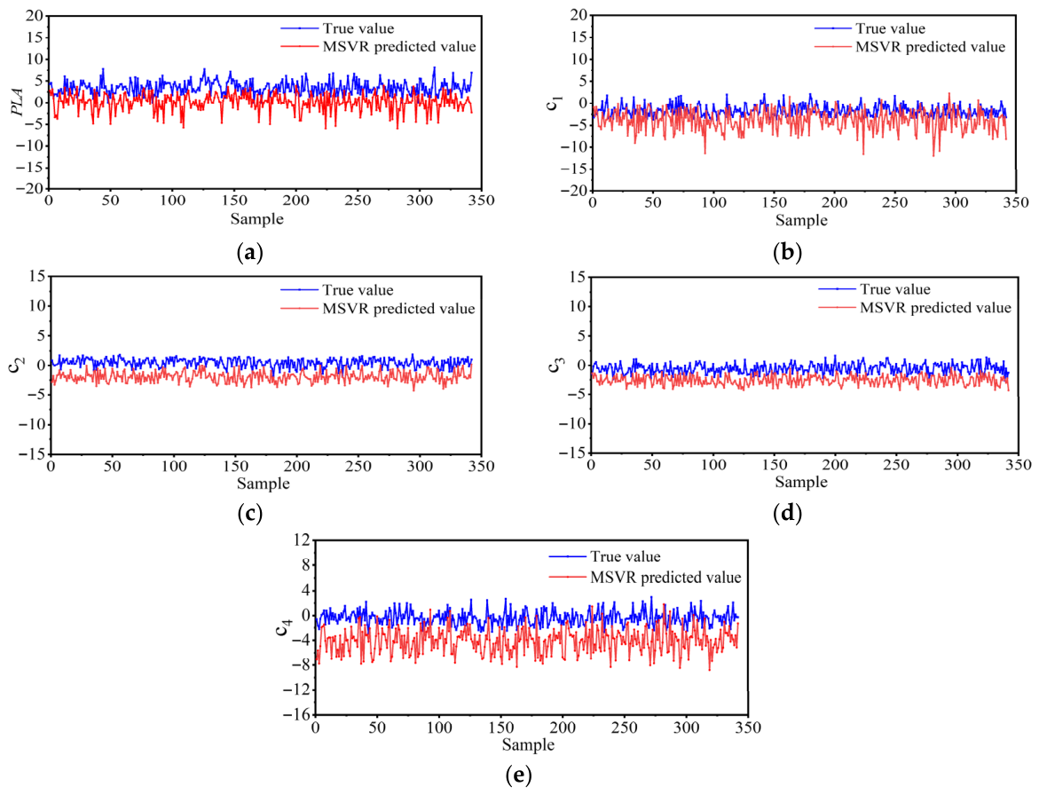
$\mathrm{M}\mathrm{S}\mathrm{V}\mathrm{R}$, $\mathrm{P}\mathrm{S}\mathrm{O}$-$\mathrm{M}\mathrm{S}\mathrm{V}\mathrm{R}$, and $\mathrm{P}\mathrm{L}\mathrm{S}$-$\mathrm{P}\mathrm{S}\mathrm{O}$-$\mathrm{M}\mathrm{S}\mathrm{V}\mathrm{R}$ are used to predict the flatness characteristic parameters of hot-rolled strip. The results of the flatness quality characteristics predicted using MSVR are shown in Figure 3. It can be seen that the predicted results are basically consistent with the true values, although they reflect a trend. However, there is still a significant deviation between the actual value and the predicted value, making it difficult to effectively reflect the true information of the flatness quality. The main reason for the occurrence of this result is that the MSVR prediction model uses kernel functions to map low-dimensional feature space vectors to high-dimensional feature spaces, in order to improve the interpretation ability of variable nonlinear relationships. However, in the prediction process, the core parameters need to be constantly corrected, which can make it difficult for the prediction model to achieve optimal results. Therefore, it is necessary to evaluate the kernel parameters of the model $\delta$ and penalty factor $C$ for optimization, to ensure the superior performance of the prediction model.

Figure 3. Prediction of plate shape feature coefficients based on MSVR. (a) PLA prediction based on MSVR; (b) c₁ prediction based on MSVR; (c) $c_2$ prediction based on $\mathrm{M}\mathrm{S}\mathrm{V}\mathrm{R}$; (d) $c_3$ prediction based on $\mathrm{M}\mathrm{S}\mathrm{V}\mathrm{R}$; (e) $c_4$ prediction based on $\mathrm{M}\mathrm{S}\mathrm{V}\mathrm{R}$.

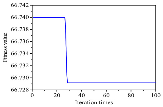
Use the particle swarm optimization to optimize the kernel parameter $\delta$ and penalty factor $C$ in the model. As shown in Figure 4, it is the fitness curve of the $\mathrm{P}\mathrm{S}\mathrm{O}$-$\mathrm{M}\mathrm{S}\mathrm{V}\mathrm{R}$ model optimization process. In the optimization process, the optimal value is found when the number of iterations is 30.

Figure 4. PSO-MSVR fitness curve.

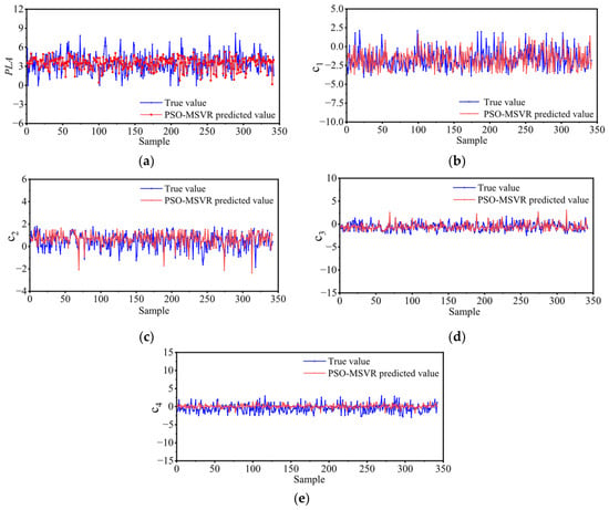
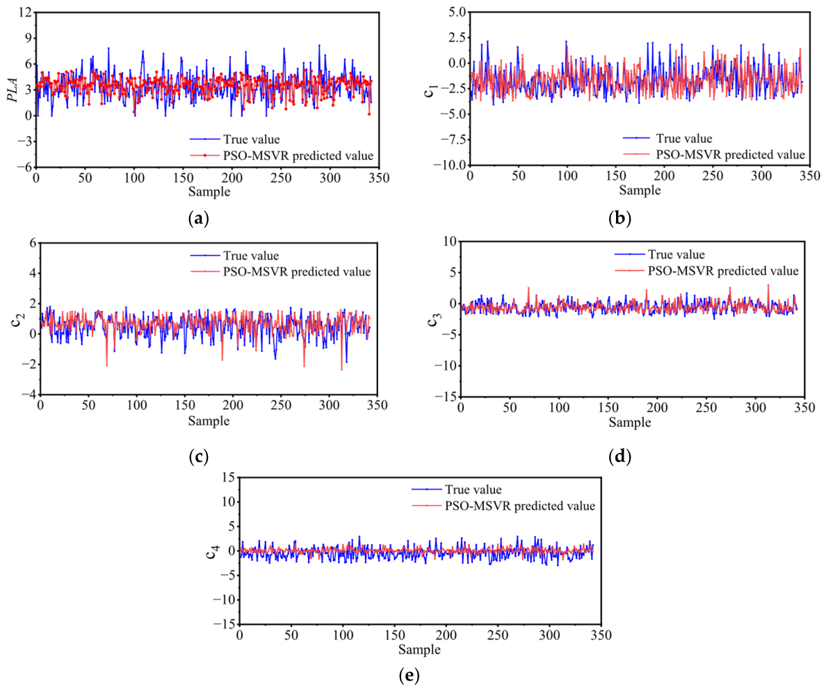
The prediction results of flatness feature coefficients based on the $\mathrm{P}\mathrm{S}\mathrm{O}$-$\mathrm{M}\mathrm{S}\mathrm{V}\mathrm{R}$ method are shown in Figure 5. The $\mathrm{P}\mathrm{S}\mathrm{O}$-$\mathrm{M}\mathrm{S}\mathrm{V}\mathrm{R}$ model has a good predictive effect on the flatness quality characteristic coefficients. It has been proven that the $\mathrm{P}\mathrm{S}\mathrm{O}$-$\mathrm{M}\mathrm{S}\mathrm{V}\mathrm{R}$ model can better fit the complex nonlinear relationship between complex rolling process technology and flatness quality characteristic coefficients, and has a good predictive effect on flatness quality.

Figure 5. Prediction of flatness feature coefficients based on PSO-MSVR. (a) $PLA$ prediction based on $\mathrm{P}\mathrm{S}\mathrm{O}$-$\mathrm{M}\mathrm{S}\mathrm{V}\mathrm{R}$; (b) $c_1$ prediction based on $\mathrm{P}\mathrm{S}\mathrm{O}$-$\mathrm{M}\mathrm{S}\mathrm{V}\mathrm{R}$; (c) $c_2$ prediction based on $\mathrm{P}\mathrm{S}\mathrm{O}$-$\mathrm{M}\mathrm{S}\mathrm{V}\mathrm{R}$; (d) $c_3$ prediction based on $\mathrm{P}\mathrm{S}\mathrm{O}$-$\mathrm{M}\mathrm{S}\mathrm{V}\mathrm{R}$; (e) $c_4$ prediction based on $\mathrm{P}\mathrm{S}\mathrm{O}$-$\mathrm{M}\mathrm{S}\mathrm{V}\mathrm{R}$.

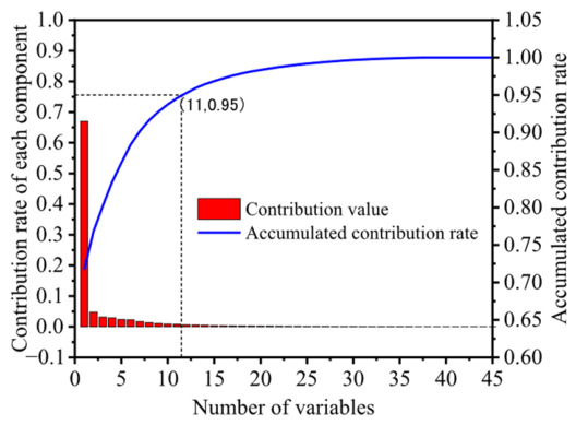
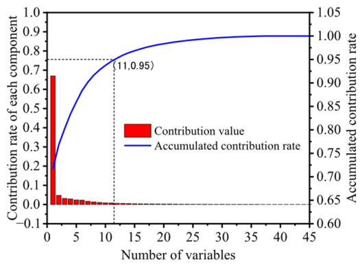
The accuracy of the optimized $\mathrm{M}\mathrm{S}\mathrm{V}\mathrm{R}$ prediction model has been improved. However, in the prediction process, it is found that the process variables are many, and the related variables are complex. There is a lot of redundant information in the prediction process of a characteristic coefficient, which reduces the accuracy of the prediction model and increases the cost of prediction time. Therefore, this article integrates the $\mathrm{P}\mathrm{L}\mathrm{S}$ algorithm with the vector machine prediction model. The $\text{PLS-PSO-MSVR}$ flatness feature prediction model was proposed to improve the prediction accuracy, reduce the dimensionality of the input data, and improve the computational efficiency of the model. The contribution rate and cumulative contribution rate of characteristic variables were calculated based on PLS, and the results are shown in Figure 6. According to the cumulative contribution rate, when the number of principal elements is 11, 95% of the variation in the original data is explained. Therefore, the extracted data features can be used as input for the prediction model of flatness feature coefficients.

Figure 6. Contribution rates of various variables.

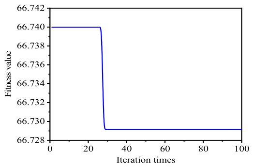
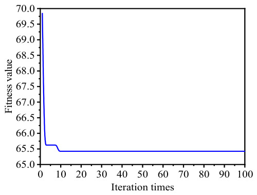
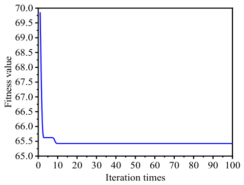
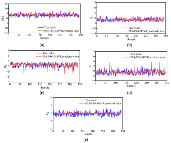
As shown in Figure 7, it is the fitness curve of the PLS-PSO-MSVR model optimization process. After feature extraction of the original data through PLS, the model found the optimal parameter value at 10 iterations, significantly reducing the number of iterations. Based on the $\mathrm{P}\mathrm{L}\mathrm{S}$-$\mathrm{P}\mathrm{S}\mathrm{O}$-$\mathrm{M}\mathrm{S}\mathrm{V}\mathrm{R}$ method, the prediction of flatness feature coefficients is shown in Figure 8.

Figure 7. $\mathrm{PLS}\text{-}\mathrm{PSO}\text{-}\mathrm{MSVR}$ fitness curve.

Figure 8. Prediction of flatness feature coefficients based on $\mathrm{P}\mathrm{L}\mathrm{S}$-$\mathrm{P}\mathrm{S}\mathrm{O}$-$\mathrm{M}\mathrm{S}\mathrm{V}\mathrm{R}$. (a) $PLA$ prediction based on $\mathrm{P}\mathrm{L}\mathrm{S}$-$\mathrm{P}\mathrm{S}\mathrm{O}$-$\mathrm{M}\mathrm{S}\mathrm{V}\mathrm{R}$; (b) $c_1$ prediction based on $\mathrm{P}\mathrm{L}\mathrm{S}$-$\mathrm{P}\mathrm{S}\mathrm{O}$-$\mathrm{M}\mathrm{S}\mathrm{V}\mathrm{R}$; (c) $c_2$ prediction based on $\mathrm{P}\mathrm{L}\mathrm{S}$-$\mathrm{P}\mathrm{S}\mathrm{O}$-$\mathrm{M}\mathrm{S}\mathrm{V}\mathrm{R}$; (d) $c_3$ prediction based on $\mathrm{P}\mathrm{L}\mathrm{S}$-$\mathrm{P}\mathrm{S}\mathrm{O}$-$\mathrm{M}\mathrm{S}\mathrm{V}\mathrm{R}$; (e) $c_4$ prediction based on $\mathrm{P}\mathrm{L}\mathrm{S}$-$\mathrm{P}\mathrm{S}\mathrm{O}$-$\mathrm{M}\mathrm{S}\mathrm{V}\mathrm{R}$.

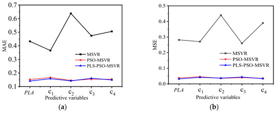
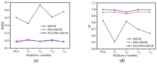
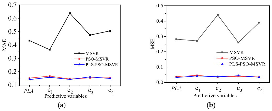
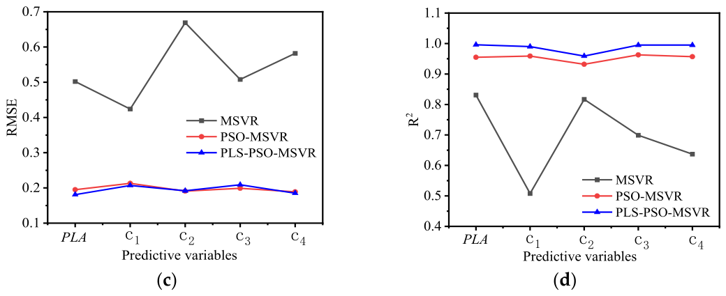
Among the three prediction models for flatness feature coefficients, the $\mathrm{M}\mathrm{A}\mathrm{E}$, $\mathrm{M}\mathrm{S}\mathrm{E}$, and $\mathrm{R}\mathrm{M}\mathrm{S}\mathrm{E}$ of $\mathrm{P}\mathrm{L}\mathrm{S}$-$\mathrm{P}\mathrm{S}\mathrm{O}$-$\mathrm{M}\mathrm{S}\mathrm{V}\mathrm{R}$ are lower than other models, and the ${\mathrm{R}}^2$ is higher than the comparison models. The $\mathrm{P}\mathrm{L}\mathrm{S}$-$\mathrm{P}\mathrm{S}\mathrm{O}$-$\mathrm{M}\mathrm{S}\mathrm{V}\mathrm{R}$ model has the smallest $\mathrm{M}\mathrm{A}\mathrm{E}$, $\mathrm{M}\mathrm{S}\mathrm{E}$, and $\mathrm{R}\mathrm{M}\mathrm{S}\mathrm{E}$ in predicting the flatness coefficients, and the average ${\mathrm{R}}^2$ reached 0.987. As shown in Figure 9, after the introduction of particle swarm optimization to optimize the model parameters, the prediction model has a good prediction accuracy. Comparing the two prediction models, $\mathrm{P}\mathrm{S}\mathrm{O}$-$\mathrm{M}\mathrm{S}\mathrm{V}\mathrm{R}$ and $\mathrm{P}\mathrm{L}\mathrm{S}$-$\mathrm{P}\mathrm{S}\mathrm{O}$-$\mathrm{M}\mathrm{S}\mathrm{V}\mathrm{R}$, the $\mathrm{M}\mathrm{A}\mathrm{E}$, $\mathrm{M}\mathrm{S}\mathrm{E}$, and $\mathrm{R}\mathrm{M}\mathrm{S}\mathrm{E}$ evaluation indicators can meet the prediction requirements, as shown in Figure 9a–c. The decision coefficient ${\mathrm{R}}^2$ evaluation index of the prediction model $\mathrm{P}\mathrm{L}\mathrm{S}$-$\mathrm{P}\mathrm{S}\mathrm{O}$-$\mathrm{M}\mathrm{S}\mathrm{V}\mathrm{R}$ has significantly improved. This prediction model can achieve complete fitting of the data relationship between the dependent variable and the independent variable.

Figure 9. Prediction and evaluation indicators for different models. (a) $\mathrm{M}\mathrm{A}\mathrm{E}$ evaluation indicator; (b) $\mathrm{M}\mathrm{S}\mathrm{E}$ evaluation indicator; (c) $\mathrm{R}\mathrm{M}\mathrm{S}\mathrm{E}$ evaluation indicator; (d) ${\mathrm{R}}^2$ evaluation indicator.

The prediction model proposed in this paper not only achieves better prediction results, but also reduces the error between the predicted value and the actual value. By feature extraction, the prediction loss time is reduced and the time cost is lower. As shown in Table 4, the $\mathrm{P}\mathrm{L}\mathrm{S}$ algorithm was used to extract the principal components of flatness-related data and construct a feature set. By reducing the dimensionality of the data, the prediction efficiency of our model was improved by 26.34% compared to the $\text{PSO-MSVR}$ model.

Table 4. Prediction time of different models.

Prediction Model	Optimization Parameter	Time (s)
$\mathrm{MSVR}$	-	5.319
$\mathrm{PSO}\text{-}\mathrm{MSVR}$	$\left(\delta ,C\right)$	22.458
$\mathrm{PLS}\text{-}\mathrm{PSO}\text{-}\mathrm{MSVR}$	$\left(\delta ,C\right)$	16.401

This article proposes to parameterize the flatness quality, extract the flatness feature coefficient, and use the flatness feature coefficient as the indicator parameter for judging flatness. The fluctuation of strip flatness can be directly characterized by characteristic parameters, which can provide reference for the diagnosis of flatness anomalies. Three prediction models were compared, including $\mathrm{M}\mathrm{S}\mathrm{V}\mathrm{R}$, $\mathrm{P}\mathrm{S}\mathrm{O}$-$\mathrm{M}\mathrm{S}\mathrm{V}\mathrm{R}$, and $\mathrm{P}\mathrm{L}\mathrm{S}$-$\mathrm{P}\mathrm{S}\mathrm{O}$-$\mathrm{M}\mathrm{S}\mathrm{V}\mathrm{R}$. The MSVR prediction model can effectively solve the high-dimensional nonlinear small-sample problem, but in the process of mapping data to high-dimensional space, the selection of kernel parameters has a certain degree of blindness, making it difficult to ensure the reliability of the prediction results. Therefore, optimizing the $\mathrm{M}\mathrm{S}\mathrm{V}\mathrm{R}$ model through the $\mathrm{P}\mathrm{S}\mathrm{O}$ algorithm in high-dimensional data reduces the blindness of the parameter search.

In the process of parameter optimization of the $\mathrm{P}\mathrm{S}\mathrm{O}$-$\mathrm{M}\mathrm{S}\mathrm{V}\mathrm{R}$ model, because there are many quality-related variables, when $\mathrm{P}\mathrm{S}\mathrm{O}$-$\mathrm{M}\mathrm{S}\mathrm{V}\mathrm{R}$ models the strip quality data, the computational complexity increases with the increase in iteration times, resulting in higher time consumption. The computational complexity of the modeling process increases with the number of iterations, resulting in higher time consumption. In this paper, considering the correlation between process variables and quality variables, combining $\mathrm{P}\mathrm{L}\mathrm{S}$ and $\mathrm{P}\mathrm{S}\mathrm{O}$-$\mathrm{M}\mathrm{S}\mathrm{V}\mathrm{R}$, a flatness quality feature prediction model of $\mathrm{P}\mathrm{L}\mathrm{S}$-$\mathrm{P}\mathrm{S}\mathrm{O}$-$\mathrm{M}\mathrm{S}\mathrm{V}\mathrm{R}$ was proposed. The $\mathrm{P}\mathrm{L}\mathrm{S}$ method was used to extract the components with strong influence on the flatness features, overcome the problem of information redundancy, reduce the dimension of the multi-output support vector machine, and shorten the execution time of modeling.

The overall structure of the proposed method can be considered as a series structure. Firstly, feature extraction is performed on the input variables, and feature data is used as input to the prediction model. Then, the iterative training process is completed through $\mathrm{P}\mathrm{S}\mathrm{O}$-$\mathrm{M}\mathrm{S}\mathrm{V}\mathrm{R}$ and parameter optimization is completed. The $\mathrm{P}\mathrm{L}\mathrm{S}$-$\mathrm{P}\mathrm{S}\mathrm{O}$-$\mathrm{M}\mathrm{S}\mathrm{V}\mathrm{R}$ model has the advantages of high prediction accuracy and efficient modeling process, which is conducive to the development of the plate-shape quality control system based on the principle of prediction feedback.

5. Conclusions

The reason for the development of $\mathrm{P}\mathrm{L}\mathrm{S}$-$\mathrm{P}\mathrm{S}\mathrm{O}$-$\mathrm{M}\mathrm{S}\mathrm{V}\mathrm{R}$ is to realize better monitoring and diagnosis of hot-rolled flatness. There are quality fluctuations and unknown reasons for abnormal flatness during the hot rolling process, making it impossible to achieve early control of flatness quality. In order to solve this problem, this paper parameterizes the flatness characteristics, takes the flatness coefficient as the prediction object, and then monitors the influence of process variables on the flatness characteristics. Considering the relationship between process variables and quality, PLS was used to extract appropriate latent variables as input variables to optimize the quality and structure of the data, and improve model prediction efficiency. The multi-output $\mathrm{M}\mathrm{S}\mathrm{V}\mathrm{R}$ model was used to integrate with $\mathrm{P}\mathrm{L}\mathrm{S}$, and $\mathrm{P}\mathrm{S}\mathrm{O}$ was used to optimize the process parameters. $\mathrm{P}\mathrm{L}\mathrm{S}$-$\mathrm{P}\mathrm{S}\mathrm{O}$-$\mathrm{M}\mathrm{S}\mathrm{V}\mathrm{R}$ has higher prediction accuracy, but also has obvious improvement on parameter optimization ability. To verify the superiority of the proposed method, $\mathrm{M}\mathrm{A}\mathrm{E}$, $\mathrm{M}\mathrm{S}\mathrm{E}$, $\mathrm{R}\mathrm{M}\mathrm{S}\mathrm{E}$, and ${\mathrm{R}}^2$ were introduced to evaluate the predictive performance.

Compared with conventional single-output models (e.g., BPNN, SVR) and PCA-based dimensionality reduction methods, the proposed PLS-PSO-MSVR model demonstrates three distinct advantages:

(1)

it preserves the correlation among multiple flatness feature coefficients through multi-output regression, avoiding information loss caused by independent predictions;

(2)

PLS-based feature extraction explicitly considers the relationship between process variables and flatness quality, leading to more interpretable latent variables; and

(3)

the PSO-optimized MSVR achieves higher prediction accuracy (MAE = 0.15, R² = 0.987) with 26.34% less computational time compared to PSO-MSVR without PLS.

Future work will focus on:

(1)

Adapting the model for different steel grades and production lines.

(2)

Exploring online learning strategies for real-time prediction.

(3)

Integrating the model into a closed-loop control system.

References

- Duan, B.W.; Wang, D.C.; Wang, G.D.; Hu, Y.X.; Xu, Y.H.; Liu, H.M. Pi-TabNet: An explainable physics-informed deep learning method for flatness prediction in cold-rolled copper strips. J. Manuf. Process. 2025, 150, 1260–1281. [Google Scholar] [CrossRef] [Scilit]
- He, A.R.; Qie, H.T.; Zhang, Y.G.; Liu, C.; Chen, C.K.; Wang, X.L. Flatness prediction and optimization control of electronic aluminum foil based on MPSO-LightGBM. Int. J. Adv. Manuf. Technol. 2025, 138, 367–384. [Google Scholar] [CrossRef] [Scilit]
- Peng, Y.; Shi, B.D.; Liu, C.Y.; Xing, J.K. Review of the integrated development of strip rolling equipment-process-product quality control. J. Mech. Eng. 2023, 59, 96–118. [Google Scholar]
- Guo, H.S.; Sun, J.L.; Peng, Y.; Wu, Z.Y.; Yang, J.H. Hot-rolled strip thickness diagnosis and abnormal transmission path identification based on sub-stand strategy and KPLS-MIC-TE. J. Frankl. Inst. 2024, 361, 106622. [Google Scholar] [CrossRef] [Scilit]
- Peng, K.X.; Zhong, H.; Zhao, L.; Xue, K.; Ji, Y.D. Strip shape modeling and its setup strategy in hot strip mill process. Int. J. Adv. Manuf. Technol. 2014, 72, 589–605. [Google Scholar] [CrossRef] [Scilit]
- Yao, C.H.; He, A.R.; Shao, J.; Zhao, J.W. A real-time quasi-3D metal flow model for hot strip rolling. Int. J. Mech. Sci. 2019, 159, 91–102. [Google Scholar] [CrossRef] [Scilit]
- Shin, J.M.; Han, S.I.; Kim, J.S. Development and experimental evaluation of strip shape prediction model for Sendzimir rolling mills. J. Iron Steel Res. Int. 2013, 20, 25–32. [Google Scholar] [CrossRef] [Scilit]
- Wang, D.C.; Liu, H.M. A model coupling method for shape prediction. J. Iron Steel Res. Int. 2012, 19, 22–27. [Google Scholar] [CrossRef] [Scilit]
- Liu, Q.; Qin, S.Z. Perspectives on big data modeling of process industries. Acta Autom. Sin. 2016, 42, 161–171. [Google Scholar]
- Gao, H.; Li, X.; Jin, S.R.; Qin, Y.M.; Cao, J.Z.; Luan, F.; Zhang, D.H. Strip deviation analysis and prediction based on time series methods in hot rolling process. J. Manuf. Process. 2024, 131, 1143–1157. [Google Scholar] [CrossRef] [Scilit]
- Dong, Z.S.; Li, X.; Luan, F.; Zhang, D.H. Prediction and analysis of key parameters of head deformation of hot-rolled plates based on artificial neural networks. J. Manuf. Process. 2022, 77, 282–300. [Google Scholar] [CrossRef] [Scilit]
- Ding, J.G.; Liu, F.L.; Du, H.Z.; Li, X.; Zhang, D.H. Research and application of flatness CPS system based on multi-source data and multi-model fusion. Steel Roll. 2022, 39, 75–83+90. [Google Scholar]
- Li, M.; Li, G.Q.; Li, X.H.; Lu, L.X.; Peter, M. Prediction of mechanical properties of hot-rolled strip steel based on XGboost and metallurgical mechanism. Phys. Met. Metallogr. 2024, 125, 1728–1738. [Google Scholar]
- Shi, K.; Wang, X.; Zheng, G.; Liu, Y.F.; Wang, D.H. Shape prediction of 20-high rolling mill based on finite element and PSO-BP method. Mach. Tool Hydraul. 2023, 51, 152–157. [Google Scholar]
- Liu, J.Y.; Song, S.N.; Wang, J.Y.; Balaiti, M.; Song, N.N. Flatness prediction of cold rolled strip based on deep neural network with improved activation function. Sensors 2022, 22, 656. [Google Scholar] [CrossRef] [Scilit]
- Zhang, Y.J.; Ding, J.G.; Sun, J.; Zhang, D.H. Prediction and online optimization of strip shape in hot strip rolling process using sparrow search algorithm-online sequential-deep multilayer extreme learning machine algorithm. Steel Res. Int. 2023, 94, 2200832. [Google Scholar] [CrossRef] [Scilit]
- Meng, L.M.; Ding, J.G.; Du, H.Z.; Dong, Z.S.; Gao, P.; Zhang, D.H. Stacking ensemble learning fused with whale optimisation algorithm based method for crown prediction of hot-rolled strip. Ironmak. Steelmak. 2024, 51, 281–296. [Google Scholar] [CrossRef] [Scilit]
- Ding, Z.Y.; Ding, C.Y.; Sun, J.; Zhang, D.H. Prediction model of cold rolled strip flatness based on CatBoost. Steel Roll. 2022, 39, 99–105. [Google Scholar]
- Li, W.G.; Xie, L.; Zhao, Y.T.; Wang, W.B. Prediction model for mechanical properties of hot-rolled strips by deep learning. J. Iron Steel Res. Int. 2020, 27, 1045–1053. [Google Scholar] [CrossRef] [Scilit]
- Peng, G.Z.; Cheng, Y.L.; Zhang, Y.F.; Shao, J.; Wang, H.W.; Shen, W.M. Industrial big data-driven mechanical performance prediction for hot-rolling steel using lower upper bound estimation method. J. Manuf. Syst. 2023, 65, 104–114. [Google Scholar] [CrossRef] [Scilit]
- Liu, M.H.; Zhang, Q. Prediction of strip crown based on support vector machine and neural network. CAAI Trans. Intell. Syst. 2022, 17, 506–514. [Google Scholar]
- Pascual, H.; Yee, X.C. Least squares regression principal component analysis: A supervised dimensionality reduction method. Numer. Linear Algebra Appl. 2021, 29, e2411. [Google Scholar] [CrossRef] [Scilit]
- Gewers, F.L.; Ferreira, G.R.; De Arruda, H.F.; Silva, F.N.; Comin, C.H.; Amancio, D.R.; Costa, L.D.F. Principal component analysis: A natural approach to data exploration. ACM Comput. Surv. 2021, 54, 70. [Google Scholar] [CrossRef] [Scilit]
- Kwak, N.; Kim, C.; Kin, H. Dimensionality reduction based on ICA for regression problems. Neurocomputing 2008, 71, 2596–2603. [Google Scholar] [CrossRef] [Scilit]
- Wang, Z.H.; Liu, Y.M.; Wang, T.; Gong, D.Y.; Zhang, D.H. Prediction model of hot strip crown based on industrial data and hybrid the PCA-SDWPSO-ELM approach. Soft Comput. 2023, 27, 12483–12499. [Google Scholar] [CrossRef] [Scilit]
- Ji, Y.F.; Song, L.B.; Sun, J.; Peng, W.; Li, H.Y.; Ma, L.F. Application of SVM and PCA-CS algorithms for prediction of strip crown in hot strip rolling. J. Cent. South Univ. 2021, 28, 2333–2344. [Google Scholar] [CrossRef] [Scilit]
- Song, L.B.; Xu, D.; Wang, X.C.; Yang, Q.; Ji, Y.F. Application of machine learning to predict and diagnose for hot-rolled strip crown. Int. J. Adv. Manuf. Technol. 2022, 120, 881–890. [Google Scholar] [CrossRef] [Scilit]
- Mishra, S.; Kumar, R.; Anindya, S.; Anish, P. Assessing the Effects of DMLS Processing Conditions on the Properties of AlSi10Mg: An Experimental and Modeling Approach. J. Mater. Eng. Perform. 2026, 35, 10070–10088. [Google Scholar] [CrossRef] [Scilit]
- Sanchez-Fernadez, M.; de-Prado-Cumplido, M.; Arenas-Garcia, J.; Perez-Cruz, F. SVM multiregression for nonlinear channel estimation in multiple-input multiple-output systems. IEEE Trans. Signal Process. 2004, 52, 2298–2307. [Google Scholar] [CrossRef] [Scilit]
- George, K.; Grace, W. Some results on Tchebycheffian spline functions. J. Math. Anal. Appl. 1971, 33, 82–95. [Google Scholar] [CrossRef] [Scilit]
- Zhang, S.; Shi, W.R.; Shi, X.; Guo, B.L. Water quality prediction based on partial least squares and support vector machine. Comput. Eng. Appl. 2015, 51, 249–254. [Google Scholar]
- Liu, M.H.; Zhang, Q.; Liu, Y.H.; Wang, W.L. A novel data-driven rolling force predictive model based on PSO-BAS-HKSVR approach. J. Comput. 2021, 32, 025–041. [Google Scholar]
- Wang, P.F.; Zhang, Z.J.; Sun, J.; Zhang, D.H.; Liu, H.M.; Gao, X.L. Flatness control of cold rolled strip based on relay optimization. Ironmak. Steelmak. 2018, 45, 166–175. [Google Scholar] [CrossRef] [Scilit]
Disclaimer/Publisher’s Note: The statements, opinions and data contained in all publications are solely those of the individual author(s) and contributor(s) and not of MDPI and/or the editor(s). MDPI and/or the editor(s) disclaim responsibility for any injury to people or property resulting from any ideas, methods, instructions or products referred to in the content. |
© 2026 by the authors. Licensee MDPI, Basel, Switzerland. This article is an open access article distributed under the terms and conditions of the Creative Commons Attribution (CC BY) license.