Comparative RSM Optimization of Deep Drawing Parameters for an AA5754-O Automotive Part Using Different Objective Functions: Q-Value and Maximum Thinning Percentage

Abstract

This study presents a comparison between the results of process parameter optimization for the deep drawing of an AA5754-O automotive fuel tank, which utilizes two different objective functions. The first objective function is the maximum thinning percentage (max. %Thinning) of the formed part, which is a conventional formability index. The second is Q-value, a metric derived from the Thinning Limit Diagram that accounts for both necking-prone (excessive thinning) and wrinkling-prone (thickening) regions. The experiments were conducted using finite element simulation to model the forming behavior under an inscribed central composite design within the response surface methodology. Three process parameters, which are well known to be important for controlling material flow and achieving a balance between wrinkling and excessive thinning in deep drawing, were varied: blank holder pressure, the height of the male drawbead, and the radius of the female drawbead. Refined second-order response surface models were developed for both objective functions. Optimization based on the response surface models showed that, for the max. %Thinning objective function, the final part exhibited 19.46% maximum thinning but suffered from substantially higher wrinkling, as indicated by a maximum thickening of 36.39%. In contrast, the Q-value-based optimization resulted in a more balanced formability condition, with maximum thinning of 21.74% and maximum thickening of 13.17%. Moreover, the normalized density of elements in the safe zone of the Thinning Limit Diagram was higher, indicating an improvement in formability robustness. Therefore, this study highlights the limitations of conventional thinning-based optimization and demonstrates the potential of the Q-value as an extended practical quantitative formability tool that can simultaneously address necking and wrinkling in sheet metal forming, as presented through the studied automotive fuel tank on behalf of complex components.

1. Introduction

Deep drawing is a sheet metal forming process commonly used to form cup-shaped components. As the term ‘deep’ implies, this process involves significant material deformation. Thickness reduction or thinning naturally occurs during the deep drawing process, regardless of the deformation severity. When thinning exceeds the material’s forming limit, necking and subsequent cracking potentially occur [1,2,3]. Hence, extensive research has investigated the influence of parameters on thinning and subsequently developed forming techniques to reduce the thinning. In this context, simulations based on finite element analysis (FEA) have been widely adopted as an efficient tool for such studies, because physical experiments are time-consuming and resource-intensive [4,5,6,7].

However, while minimizing the maximum thinning value, wrinkling issues were observed as a trade-off defect in some studies, like in a deep-drawn square medical container by Taşkın and Dengiz [8] and in a fuel container by Leelaseat et al. [9]. Therefore, they concluded that minimizing the thinning value alone is insufficient for achieving optimal formability. Similarly, Kakandikar and Nandedkar [10] studied an automotive sealing cover. Although they confirmed the effectiveness of thinning-value optimization through the absence of cracking on a strain-based Forming Limit Diagram (ε-FLD), the diagram exhibited strain paths within the wrinkling zone.

In practical sheet-metal formability assessment, the thinning value serves as a conventional quantitative metric suitable for optimization. This metric is often used in conjunction with the Forming Limit Diagram, which is typically applied qualitatively to visually identify safe regions and zones at risk of necking or wrinkling. Recognizing the trade-off between thinning and wrinkling, researchers have developed objective functions to evaluate formability in a more balanced manner. Guo et al. [11] introduced an objective function based on thickness variation relative to the initial blank thickness. Positive thinning and negative thinning (thickening) correspond to necking and wrinkling, respectively. Jakumeit et al. [12] proposed an objective function that incorporates the material’s limits directly based on ε-FLD. The objective function was calculated from summing the ratio of elements located within defined ‘bad zones’ associated with necking and wrinkling. Subsequently, Kahhal et al. [13] introduced an objective function that is calculated based on the distance between the major strain of each element and the corresponding limit curves. Building upon these concepts, Leelaseat et al. [14] introduced Q-value, an objective function derived from the Thinning Limit Diagram. This diagram is obtained by transforming the conventional ε-FLD from the principal strain space into the space of engineering minor strain and thinning. As a result, both necking (represented by positive thinning) and wrinkling (represented by negative thinning) are evaluated through a unified thickness-based approach that integrates the material’s forming limits.

In the present study, a comparative optimization analysis of an AA5754-O automotive component under deep drawing is presented by evaluating the results obtained from two distinct objective functions: maximizing the Q-value and minimizing the maximum thinning percentage. To our knowledge, a direct comparison between these two approaches within a single study under the same problem scenario has yet to be reported; as such, this research investigates whether conventional thinning-based optimization leads to an unintended trade-off with wrinkling, and how the Q-value handles the trade-off. Moreover, owing to the fundamental differences in the nature of these objective functions, the results of both optimizations are analyzed using maximum thinning, maximum thickening (to monitor wrinkling), and Thinning Limit Diagrams (TLDs), in order to ensure unbiased evaluations.

The optimization in this work utilizes a design of experiments (DOE) approach based on response surface methodology (RSM) to identify the global optimum. As a widely recognized methodology in sheet-metal forming research [15,16,17,18], RSM is utilized for systematically designing experiments and modeling the relationships between input variables and responses (objective function values). Furthermore, it facilitates the interpretation of variable–response interactions through graphical representations, such as three-dimensional response surfaces and two-dimensional contour plots [19].

Regarding the selection of input variables, the present study focuses on the design feasibility stage, a critical phase occurring before the forming tools are fabricated. Since tooling represents a major capital investment, finite element simulation is employed to mitigate the risks associated with costly trial-and-error processes. In this industrial context, although various parameters influence drawability, such as frictional conditions [20,21], forming temperature [22,23], and predefined constraints including initial blank thickness [24] and material anisotropy [25], this study prioritizes parameters that are directly related to tool design and significantly impact the characteristic trade-off between thinning and wrinkling.

The drawbead geometry was selected as a primary variable because it is an integral component of the forming tools. It is typically positioned on the blank holder and the upper/lower die surface, and serves to control material flow in non-axisymmetric parts during deep drawing. A drawbead consists of a pair of opposing features: the male bead (protrusion) and the female bead (groove), which locally regulate material flow by inducing repeated bending and unbending as the blank passes through the drawbead radii. In this work, a semi-circular drawbead was employed, as it is conventionally adopted in industrial practice [26]. Existing research [27,28,29] has demonstrated that the male bead height and the female bead radius of a semi-circular drawbead are critical geometric parameters that require careful balancing. Excessive restraining force induces thinning and potential failure, whereas insufficient restraint reduces the effectiveness of wrinkling mitigation.

Since the drawbead is positioned on the blank holder, the blank holder is a fundamental forming component in deep drawing for regulating material flow in the flange region. This regulation is essential to prevent wrinkling caused by circumferential compression. Numerous studies ranging from laboratory-scale experiments to industrial deep-drawn components [30,31,32,33,34] have demonstrated that the blank holder load must be carefully controlled. An excessive load overly restricts material flow and leads to necking or cracking. In contrast, an insufficient load fails to effectively suppress wrinkling. In this industrial case study, the deep drawing process is carried out on a hydraulic press equipped with a hydraulic cushion. Consequently, the load-controlled parameter is designated as pressure. Accordingly, the blank holder pressure was selected as an investigated variable alongside the drawbead dimensions. In summary, three input variables, including the male bead height, the female bead radius, and the blank holder pressure, were selected for optimization in this study.

2. Studied Part and Material

The studied part is an automotive fuel tank made from AA5754-O sheet metal with a 1.50 mm nominal thickness. The material was selected because aluminum alloys sheet is a lightweight material, characterized by corrosion resistance via oxidation, and competitive crashworthiness relative to steel [35,36]. Specifically, AA5xxx (Al-Mg) series alloys are known for their good weldability and chemical resistance, making them suitable for fuel container applications [37]. Furthermore, the annealed condition (denoted by the -O temper) provides enhanced ductility, which is crucial for forming processes, resulting from microstructural evolution induced by heat treatment [38].

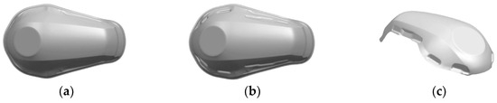
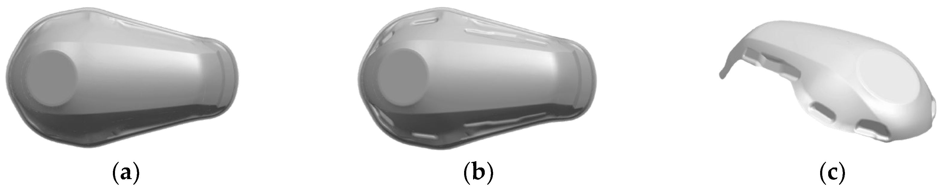
The forming process is conducted under cold forming. It involves mainly deep drawing to form the body of the part, followed by a minor stamping to form the sunken regions on the sides. The CAD models of the lower punch, corresponding to these consecutive shaping stages, are illustrated in Figure 1a,b. Finally, the flange area is removed by three-dimensional laser trimming, yielding the finished part shown in Figure 1c.

Figure 1. CAD models of the lower punch for (a) deep drawing; (b) stamping side sunken regions; (c) the final flange-trimmed part.

2.1. Material Characterization

The mechanical properties of the AA5754-O were evaluated using uniaxial tensile tests performed on an AG-X Plus 100 kN universal testing machine (SHIMADZU, Kyoto, Japan) with a strain rate of 0.001 s⁻¹. The specimen geometry was prepared according to the ASTM E8 [39] standard by wire electrical discharge machining. To characterize the material’s anisotropy, tests were conducted along three directions relative to the rolling direction (RD): 0°, 45°, and 90°, with three replicates per direction. The Lankford’s coefficients (r-values) were determined in accordance with the ASTM E517 [40] standard. The evaluated mechanical properties are summarized in Table 1.

Table 1. Mechanical properties of the AA5754-O.

Property [Unit]	Value
Young’s modulus [GPa]	70.24
Yield strength [MPa]	100.17
Ultimate tensile strength [MPa]	207.64
Total elongation [%]	21.87
Lankford’s coefficients [-]	r0	0.57
	r45	0.80
	r90	0.68

2.2. Material Modeling

2.2.1. Constitutive Modeling

In this study, the plastic deformation behavior of the material was modeled using the Swift hardening model and the YLD89 anisotropic yield criterion.

The Swift hardening model [41] is a widely used power-law model that has been proven effective in characterizing the plastic flow of AA5754-O sheets [42,43,44]. The model is expressed as shown in Equation (1).

$$\stackrel{-}{\mathsf{\sigma }} =K({{\mathsf{\epsilon }}_{0 }+\stackrel{-}{\mathsf{\epsilon }})}^n,$$

(1)

where $\stackrel{-}{\mathsf{\sigma }}$ and $\stackrel{-}{\mathsf{\epsilon }}$ denote effective stress and effective strain, respectively. The parameters $K$, $n$, and ${\mathsf{\epsilon }}_{0 }$ represent the strength coefficient, the strain hardening exponent, and the pre-strain term.

The YLD89 yield criterion [45] is a non-quadratic yield function that incorporates a crystallographic exponent ($M$), as shown in Equation (2). This model has been widely used in sheet metal forming research [46,47] due to its ability to provide reasonably accurate predictions of strain terms for highly anisotropic materials using only uniaxial tensile test data. Consequently, this model is practical for industrial applications, as the uniaxial tensile test is a universal test for characterizing material mechanical properties [48]. This facilitates parameter identification through a less specialized and less time-consuming experimental setup, making it accessible for routine industrial practice. While more recent anisotropic yield criteria, such as YLD2000 [49] and YLD2004 [50], offer enhanced predictive accuracy in yielding behavior and evolution of Lankford’s coefficients [51,52,53,54], they require a larger number of material parameters. Moreover, these parameters involve more complex identification procedures and require specialized experiments, such as balanced biaxial deformation tests. Furthermore, previous studies on aluminum alloy sheets have demonstrated that the YLD89 model strikes a superior balance between user-friendliness and predictive accuracy compared to well-known traditional quadratic model such as Hill’s 1948 [55] (which also relies solely on uniaxial data) [53,56].

$$2{\stackrel{-}{\mathsf{\sigma }}}^M = {a\left|k_1+k_2\right|}^M+{a\left|k_1-k_2\right|}^M+c{\left|{2k}_2\right|}^M,$$

(2)

The YLD89 model accounts for plane-stress components through stress invariants $k_1$ and $k_2$ as expressed in Equation (3).

$$k_1=\frac{{\mathsf{\sigma }}_{\mathit{xx}}+h{\mathsf{\sigma }}_{\mathit{yy}}}{2} \mathrm{and} k_2= \sqrt{{\left(\frac{{\mathsf{\sigma }}_{\mathit{xx}}- h{\mathsf{\sigma }}_{\mathit{yy}}}{2}\right)}^{2 }+{ p}^2{\mathsf{\sigma }}_{\mathit{xy}}^2}$$

(3)

The anisotropic parameters ($c$, $a$, $h$, and $p$) are derived from experimental Lankford’s coefficients and yield strength under uniaxial (YS) and pure shear (${\mathsf{\tau }}_1$) through the relationships in Equation (4).

$$\begin{array}{c}c=2\times \sqrt{\frac{{\mathrm{r}}_0}{1+{\mathrm{r}}_0}\times \frac{{\mathrm{r}}_{90}}{{1+\mathrm{r}}_{90}}},\\ a=2-c,\\ h=\sqrt{\frac{{\mathrm{r}}_0}{1+{\mathrm{r}}_0}\times \frac{1+{\mathrm{r}}_{90}}{{\mathrm{r}}_{90}}},\\ \mathrm{and} p=\frac{\mathrm{YS}}{{\mathsf{\tau }}_1}\times {\left(\frac{2}{2a+\left(2^{M}c\right)}\right)}^{1/M}\end{array}$$

(4)

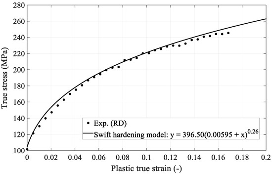
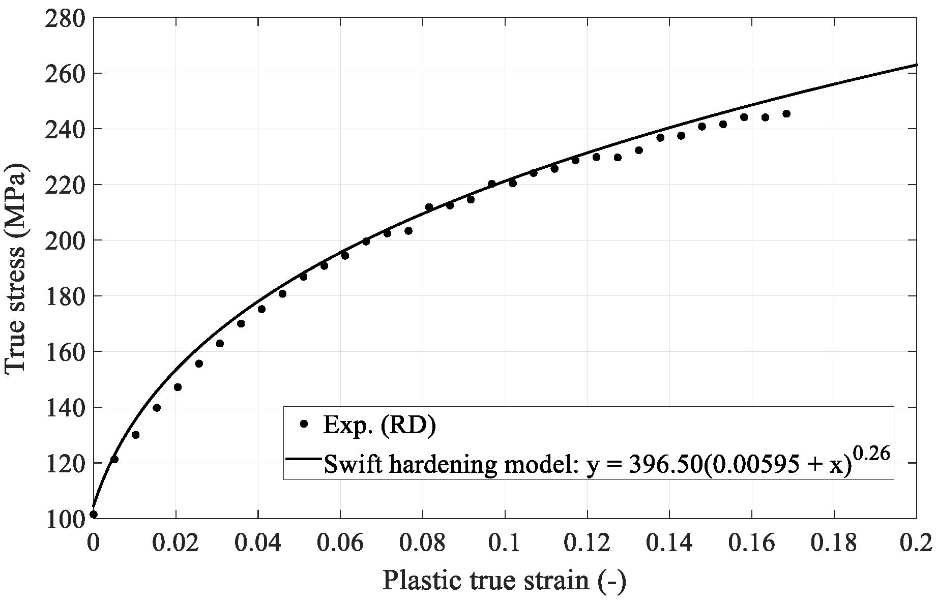
The experimental flow curve obtained from the uniaxial tensile tests was fitted to the Swift hardening model using the Curve Fitter app in MATLAB R2022b, yielding an R-squared value of 0.9963. This high correlation between the experimental true stress–strain data and the fitted curve is illustrated in Figure 2. Following the hardening model fitting and the parameter calculations described above, the identified parameters for both the Swift hardening and the YLD89 models are summarized in Table 2.

Figure 2. Experimental true stress–strain data and the fitted Swift hardening curve.

Table 2. Material parameters for the Swift hardening model and the YLD89 yield criterion.

Model	Parameter	Value [Unit]
Swift hardening	$K$	396.50 [MPa]
	${\mathsf{\epsilon }}_{0 }$	0.00595 [-]
	$n$	0.26 [-]
YLD89	$M$	8.00 [-]
	$c$	0.77 [-]
	$a$	1.23 [-]
	$h$	0.95 [-]
	$p$	1.07 [-]

2.2.2. Forming Limit Criteria

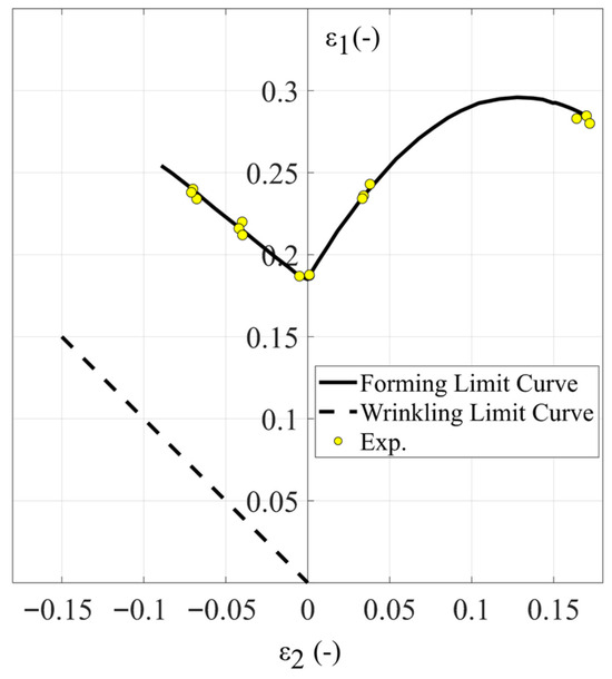
In this study, the strain-based Forming Limit Curve is utilized as the material necking criterion. The curve was determined through the Nakajima stretching tests in accordance with the ISO 12004 standard [57]. Five different waisted specimen geometries were prepared to represent different failure strain states.

The specimens were fabricated using wire electrical discharge machining. Following the methodology described by Larpprasoetkun et al. [58], a 2 mm square grid was applied via laser marking. The tests were performed on an Erichsen machine utilizing a 100 mm diameter hemispherical punch (Erichsen GmbH & Co. KG, Hemer, Germany), with a punch velocity of 1 mm/s and a maximum clamping force of 400 kN. The punch travel continued until crack initiation was observed. Subsequently, the major and minor strains (ε₁ and ε₂) were measured. The results were analyzed to construct the Forming Limit Curve, as presented in Figure 3.

Figure 3. Forming and Wrinkling Limit Curves of the AA5754-O.

In addition to the necking criterion, the dashed line in Figure 3 is adopted as the wrinkling-risk criterion. This line theoretically represents the state of pure shear, corresponding to a strain ratio of −1 (where ε₁ = −ε₂). This approach is consistent with experimental observations [59,60,61], which indicate that strain paths extending beyond this boundary into the compression-dominated region represent a wrinkled state. In this study, this criterion is utilized to identify wrinkled regions in the final formed components at the end of the finite element simulations, an approach that is commonly adopted in previous studies [62,63,64].

3. Methods

3.1. Overview of Framework

The methodology presented in this article facilitates a comparative analysis of the optimization results for the studied parameters based on two distinct objective functions: the Q-value and the maximum thinning percentage of the deep-drawn part. Finite element simulation is used as the primary experimental tool. Response surface methodology is applied to design experiments and investigate the relationship between the input variables (the studied parameters) and their corresponding responses (objective functions). Subsequently, optimization is performed independently for each objective function using regression response surface models to identify the optimal parameter conditions for: (1) minimizing the maximum thinning percentage, and (2) maximizing the Q-value. Finally, the results from both optimizations, consisting of the maximum thinning and thickening values on the simulated parts, and Thinning Limit Diagram characteristics, are compared and interpreted.

3.2. Response Surface Methodology Implementation

RSM was implemented in a sequential manner following established frameworks [65]. The input variables and responses are presented in Section 3.2.1 and Section 3.2.2. The experimental design and the subsequent parametric modeling for response surface fitting are described in Section 3.2.3 and Section 3.2.4, respectively.

3.2.1. Input Variables

Based on the selection criteria established in Section 1 (Introduction), this study investigates three primary input variables. These parameters include the blank holder pressure (BHP) along with the male bead height (H_{male bead}) and the female bead radius (R_{female bead}) of the semi-circular drawbead.

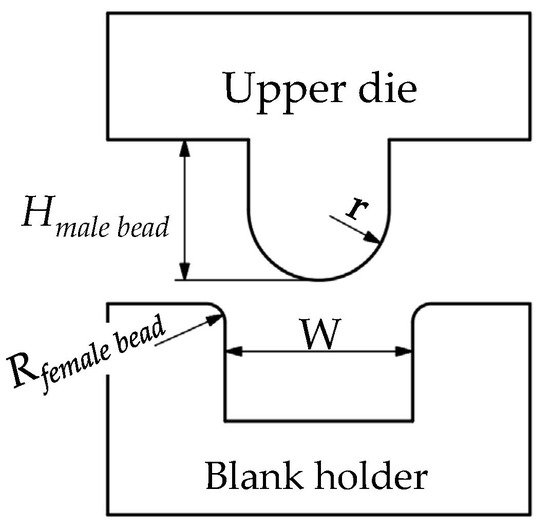
The configuration of the semi-circular drawbead is illustrated in the schematic cross-section in Figure 4. The male bead is integrated into the upper die, while the female bead groove is integrated into the blank holder. To ensure consistency in the analysis of the designated input variables, the width of the female groove (W) and the radius of the male bead (r) are fixed at 13.50 mm and 4.50 mm, respectively. The specific experimental ranges for the independent variables are detailed in Table 3.

Figure 4. Schematic of the semi-circular drawbead.

Table 3. Experimental ranges of the input variables.

Parameter [Unit]	Symbol	Levels
		Low	High
Blank holder pressure [MPa]	BHP	0.30	0.60
Male bead height [mm]	Hmale bead	2.25	4.50
Female bead radius [mm]	Rfemale bead	4.50	9.00

3.2.2. Responses and Q-Value Assessment

The maximum thinning percentage (max. %Thinning) and the Q-value are the selected responses used to evaluate the formability of the flange-trimmed part (illustrated in Figure 1c). These responses are extracted from the finite element simulation results, which are based on the predicted strain distribution of the deformed material under the influence of the forming process. While max. %Thinning is directly obtained from the simulation results, the Q-value requires additional computation based on the simulation output.

The Q-value is a quantitative metric for formability assessment derived from the Thinning Limit Diagram (TLD) [14]. While inspired by the conventional strain-based Forming Limit Diagram (ε-FLD), the TLD addresses both necking and wrinkling risks within a unified thickness-based framework. The transformation from the conventional major–minor strain space to the engineering minor strain (e₂)–thinning space is based on the assumption of material volume constancy during plastic deformation, as formulated in Equation (5). The principal strain in the thickness direction (ε₃) is calculated using the in-plane principal strains (ε₁ and ε₂) obtained from the ε-FLD, which incorporates the strain path, the Forming Limit Curve, and the Wrinkling Limit Curve. To avoid confusion with conventional strain-based diagrams, the converted FLC within the TLD is hereafter referred to as the Thinning Limit Curve (TLC).

$$\left.\%\mathrm{Thinning}=100\%\times (1-e^{-({\mathrm{\epsilon }}_1+{\mathrm{\epsilon }}_2)}\right)$$

(5)

The Q-value framework is grounded in the principle of material inhomogeneity, whereby thickness variations lead to a reduction in the forming limit. This phenomenon is well described by the Marciniak–Kuczynski (M-K) model [66]. The model assumes the existence of a pre-existing imperfection or a thinner region within the material that eventually leads to localized necking under load. As the thickness ratio decreases, the FLCs generated by the M-K model shift downward, signifying a lower necking threshold. Such theoretical behavior is consistent with experimental observations in aluminum alloys such as AA5083 [67]. Furthermore, it is supported by stepped-tensile specimen tests [68], which demonstrate that a greater difference between two connected cross-sectional areas results in lower total elongation.

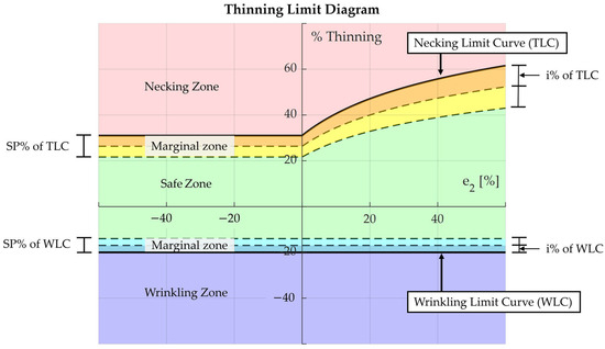
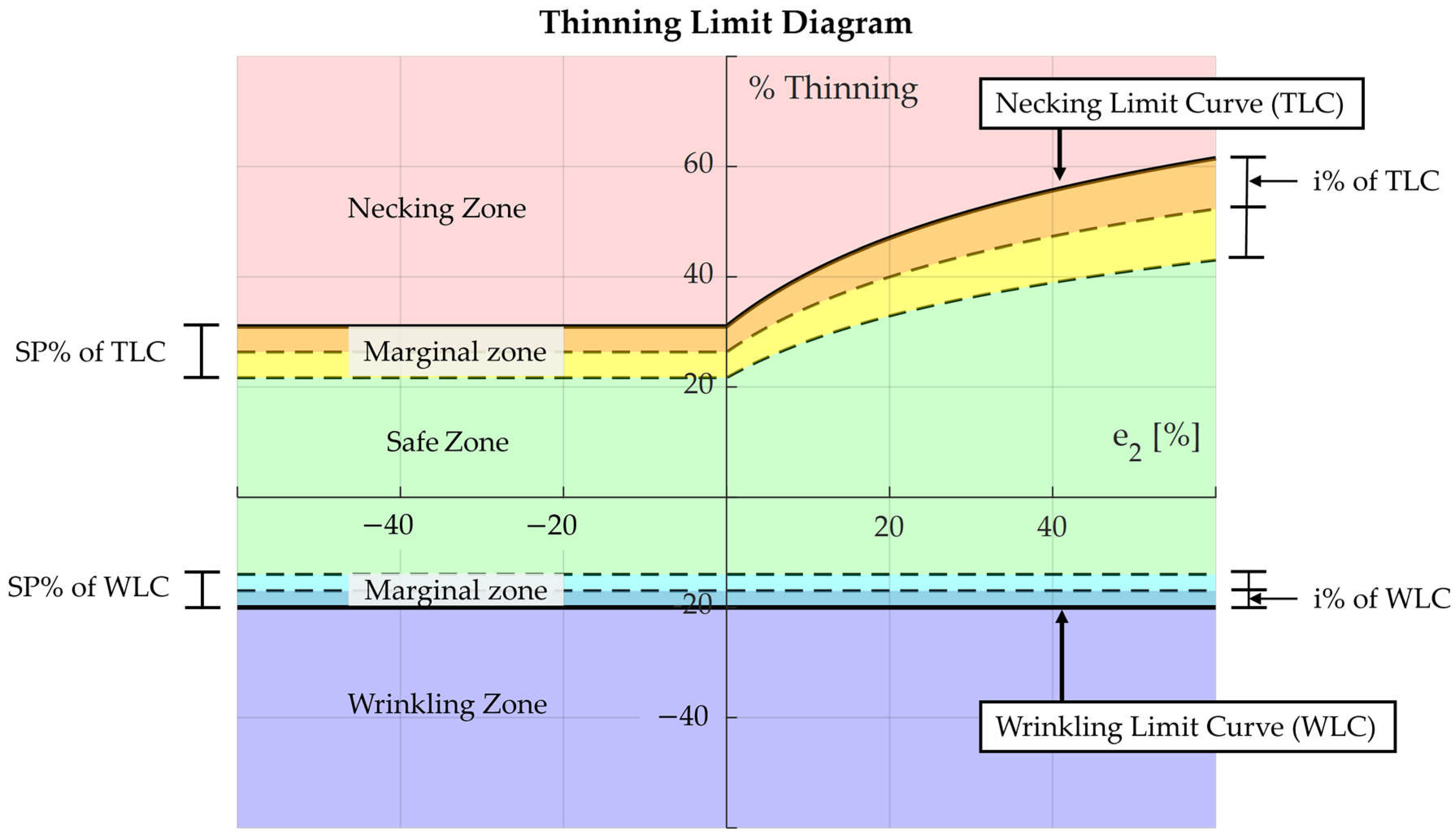
Consequently, in the Q-value formability assessment framework, the proximity of the thinning state to the TLC and the degree of material thickening as it approaches the wrinkling limit serve as quantitative indicators of severity. As illustrated in Figure 5, both the TLC and WLC are offset into multiple severity levels within marginal zones.

Figure 5. Thinning Limit Diagram with severity levels for Q-value assessment (Reprinted from Ref. [14]).

The width of these zones is defined by the severity percentage (SP%) and the interval width (i%). These marginal zones are located between the safe zone at the center and the necking or wrinkling zones at the outermost levels. The total number of intervals is determined by Equation (6), in which the value of three represents the intervals for the necking, safe, and wrinkling zones.

$$\mathrm{Number} \mathrm{of} \mathrm{intervals}=({\displaystyle \frac{\mathrm{SP}\%}{\mathrm{i}\%}} \times 2)+3$$

(6)

The Q-value is calculated by a weighted summation of the normalized number of elements in each level using the Pascal weighting factor (${\mathrm{W}}_{\mathrm{k}}$), as shown in Equation (7).

$$\mathrm{Q}-\mathrm{value}={\sum }_{\mathrm{k}=1}^{\mathrm{Number} \mathrm{of} \mathrm{intervals}}\left({\mathrm{W}}_{\mathrm{k}}\times ({\displaystyle \frac{\mathrm{number} \mathrm{of} \mathrm{elements} \mathrm{in} \mathrm{interval} \mathrm{kth}}{\mathrm{total} \mathrm{number} \mathrm{of} \mathrm{elements}}})\right)$$

(7)

In this formulation, $\mathrm{k}$ is an integer in the range from 1 to the Number of intervals. The zones are ordered from the critical necking zone ($\mathrm{k}=1$) at the top level down to the wrinkling zone at the final interval. ${\mathrm{W}}_{\mathrm{k}}$ is calculated using Equation (8), where $\mathrm{n}$ represents the Number of intervals minus 1.

$${\mathrm{W}}_{\mathrm{k}}={\displaystyle \frac{\mathrm{n}!}{(\mathrm{n}-(\mathrm{k}-1\left)\right)!\times (\mathrm{k}-1)!}}$$

(8)

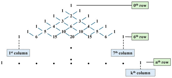
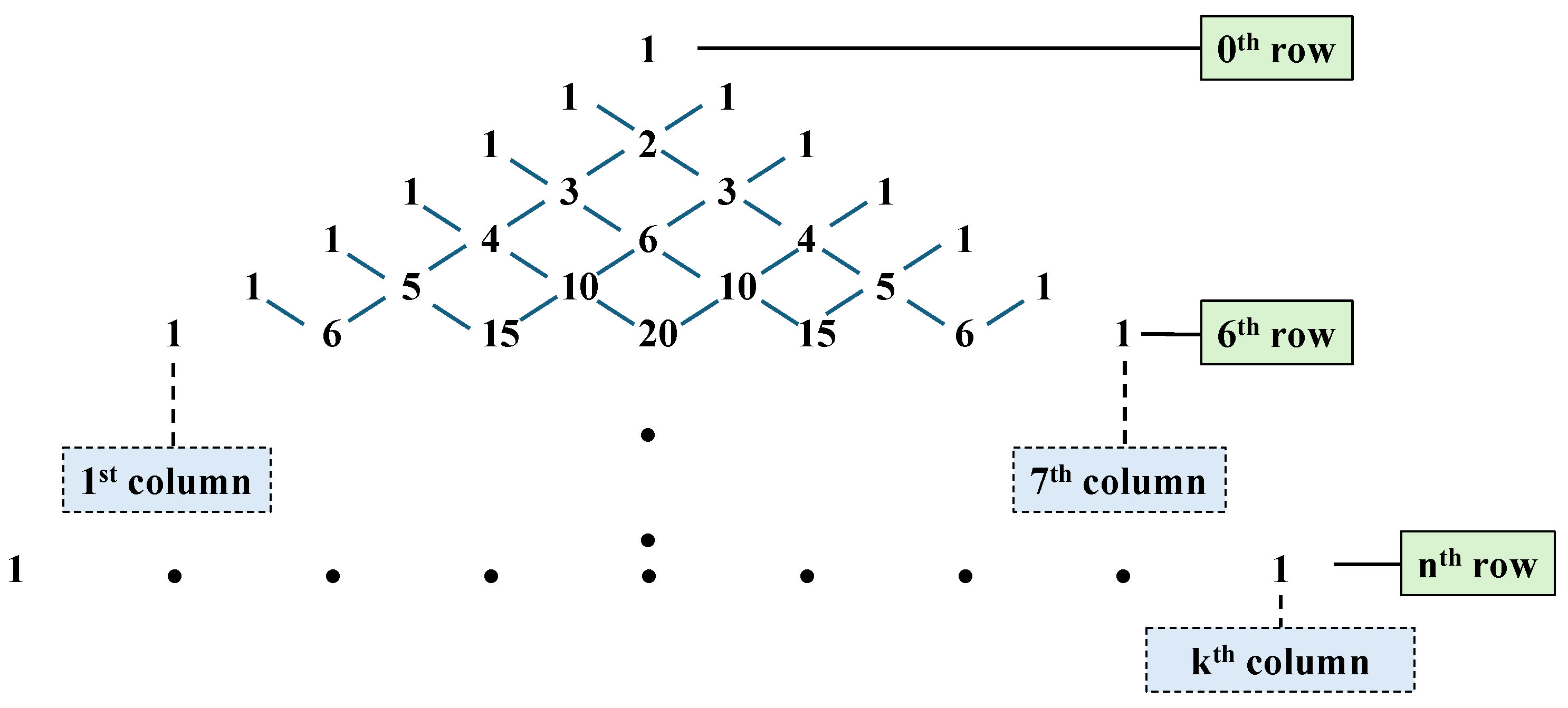
The mathematical properties of Pascal’s triangle, as illustrated in Figure 6, provide the theoretical foundation for the Q-value weighting scheme. The coefficients in each row exhibit inherent symmetry, a characteristic that ensures the risks of necking and wrinkling are balanced during the weighting process. Furthermore, the binomial distribution inherent in Pascal’s triangle approximates a normal distribution as the number of intervals increases [69]. As depicted in Figure 6, this behavior resembling a normal distribution becomes apparent from the sixth row onward. This statistical basis enables the weighting scheme to represent the severity of each level effectively without bias toward any specific interval.

Figure 6. Pascal’s triangle coefficients in nth row and kth column.

By leveraging the distribution in Pascal’s triangle, the strategy assigns the highest weighting factors to the safe zone, which progressively decrease toward a minimum value of 1 at the levels of necking and wrinkling. Consequently, a higher Q-value indicates a superior degree of formability because it reflects a larger proportion of elements residing within the safe region of the TLD. Notably, this Q-value metric is not a universal empirical constant; instead, it represents a physically meaningful assessment that is comparable within the same research framework defined by the SP%, i%, and specific experimental settings.

The flexibility of this weighting strategy is a key advantage of the Q-value framework, as it supports user-defined configurations tailored to specific problem requirements. In this study, the value of SP% is set to 20% because the maximum tolerance for thinning and thickening in the automotive manufacturing industry is conventionally 20% [70,71]. This value is also consistent with the specifications of the manufacturer collaborating in this study.

The interval width (i%) is set to 5% to provide an appropriate resolution *. According to Equation (6), this configuration results in 11 severity intervals where $\mathrm{n}=10$. This $\mathrm{n}$ value corresponds to the 10th row of Pascal’s triangle, which approximates a normal distribution. The specific Pascal weighting factors (${\mathrm{W}}_{\mathrm{k}}$) and their corresponding thinning ranges are detailed in Table 4.

Table 4. Weighting factors and associated thinning intervals for Q-value calculation.

${\mathrm{W}}_{\mathrm{k}}$	Condition
1	TLC(e2) ≤ %Thinning(e2)
10	0.95TLC(e2) ≤ %Thinning(e2) < TLC(e2)
45	0.90TLC(e2) ≤ %Thinning(e2) < 0.95TLC(e2)
120	0.85TLC(e2) ≤ %Thinning(e2) < 0.90TLC(e2)
210	0.80TLC(e2) ≤ %Thinning(e2) < 0.85TLC(e2)
252	0 ≤ %Thinning(e2) < 0.80TLC(e2)
210	−5 ≤ %Thinning(e2) < 0
120	−10 ≤ %Thinning(e2) < −5
45	−15 ≤ %Thinning(e2) < −10
10	−20 ≤ %Thinning(e2) < −15
1	%Thinning(e2) < −20

* Note: This selection was made to preserve the interpretability of the Q-value. An excessively high i% (e.g., 10%) would yield insufficient resolution, failing to distinguish critical near-failure states from highly safe states. Conversely, an overly low i% (e.g., 1%) would result in 43 intervals ($\mathrm{n}=42$), where the peak Pascal coefficient reaches a prohibitive 133 trillion (133,354,185,630,760). Such extreme magnitude could lead to difficulties in interpretation. Thus, while SP% is dictated by manufacturing standards, i% is a parameter limited by the need for appropriate severity classification without over-refinement, coupled with maintaining an $\mathrm{n}$ value of at least 6 to allow the weighting distribution to effectively approximate a normal model. The sensitivity of the framework to these parameters represents an intriguing challenge, offering a compelling pathway for future research to formalize standardized selection criteria.

3.2.3. Design of Experiments

The central composite design (CCD) is a well-established design used to support multivariate optimization within an RSM framework [72]. This design incorporates axial points positioned at an equal distance from the center for all variables to ensure rotatability [73].

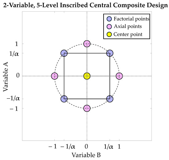
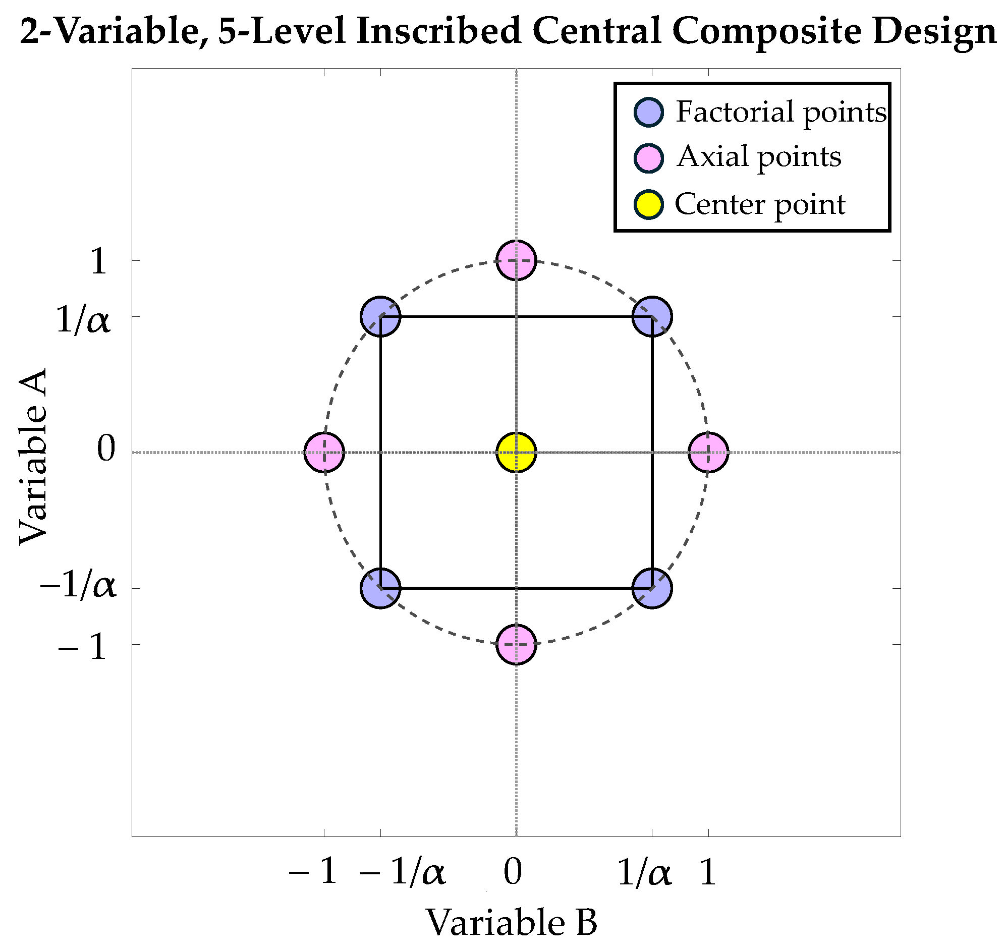
Owing to engineering constraints such as equipment capabilities, safety requirements, and resource limitations, the inscribed central composite design (CCI) is applied to ensure that all experimental points are located within the original variable range. As illustrated in Figure 7 for a two-variable example, the axial points are fixed at coded units of ±1, while the factorial points are positioned within these limits at ±1/$\alpha$. The value of $\alpha$ is calculated based on the number of variables ($k$) as shown in Equation (9).

$$\alpha ={\left(2^{\mathit{k}}\right)}^{1/4}$$

(9)

Figure 7. Illustration of a two-variable, five-level inscribed central composite design.

To eliminate scale dependency between variables with different units and ranges, the input variables are normalized from natural units (X_i) into dimensionless coded units (x_i) according to Equation (10).

$${\mathrm{x}}_{\mathrm{i}}=({\mathrm{X}}_{\mathrm{i}}-{\mathrm{X}}_{0, \mathrm{i}})/∆{\mathrm{X}}_{\mathrm{i}}$$

(10)

where X_{0, i} is the value at the center point, representing the mean of the variable’s range, and $∆$X_i is half of the variable’s range.

The experimental variables and their respective levels for the three-factor, five-level CCI design employed in this study are summarized in Table 5.

Table 5. Experimental design matrix for the inscribed central composite design.

Condition Number	Coded Unit (BHP, Hmale bead, Rfemale bead)	BHP [MPa]	Hmale bead  [mm]	Rfemale bead  [mm]	Point Type
1	(−0.595, −0.595, −0.595)	0.36	2.71	5.41	Factorial
2	(0.595, −0.595, −0.595)	0.54	2.71	5.41	Factorial
3	(−0.595, −0.595, 0.595)	0.36	2.71	8.09	Factorial
4	(0.595, −0.595, 0.595)	0.54	2.71	8.09	Factorial
5	(−0.595, 0.595, −0.595)	0.36	4.04	5.41	Factorial
6	(0.595, 0.595, −0.595)	0.54	4.04	5.41	Factorial
7	(−0.595, 0.595, 0.595)	0.36	4.04	8.09	Factorial
8	(0.595, 0.595, 0.595)	0.54	4.04	8.09	Factorial
9	(0, 0, 0)	0.45	3.38	6.75	Center 1
10	(0, 0, 0)	0.45	3.38	6.75	Center 2
11	(0, 0, 0)	0.45	3.38	6.75	Center 3
12	(0, −1, 0)	0.45	2.25	6.75	Axial
13	(0, 1, 0)	0.45	4.50	6.75	Axial
14	(0, 0, −1)	0.45	3.38	4.50	Axial
15	(0, 0, 1)	0.45	3.38	9.00	Axial
16	(−1, 0, 0)	0.30	3.38	6.75	Axial
17	(1, 0, 0)	0.60	3.38	6.75	Axial
18	(0, 0, 0)	0.45	3.38	6.75	Center 4
19	(0, 0, 0)	0.45	3.38	6.75	Center 5
20	(0, 0, 0)	0.45	3.38	6.75	Center 6

Note: The factorial points: coded unit of ±1/$\alpha$ $\approx$ ±0.595.

3.2.4. Response Surface Modeling

Since the true functional relationship between the independent variables and the responses is generally unknown, an empirical model is required to approximate this relationship within the investigated design space. Various parametric models, such as first-order models, interaction models, and higher-order polynomials, are typically available for this purpose. However, the second-order response surface model has demonstrated superior effectiveness across various engineering research fields due to its relative simplicity in fitting and its capability to capture non-linear behaviors [74,75,76,77].

Consequently, this study adopts the second-order response surface model for three variables ($k=3)$ as expressed in Equation (11).

$$\hat{y}={\mathrm{b}}_0+{\mathrm{b}}_1{\mathrm{x}}_1+{\mathrm{b}}_2{\mathrm{x}}_2+{\mathrm{b}}_3{\mathrm{x}}_3+{\mathrm{B}}_{12}{\mathrm{x}}_1{\mathrm{x}}_2+{\mathrm{B}}_{13}{\mathrm{x}}_1{\mathrm{x}}_3+{\mathrm{B}}_{23}{\mathrm{x}}_2{\mathrm{x}}_3+{\mathrm{B}}_{11}{{\mathrm{x}}_{1^1}+\mathrm{B}}_{22}{\mathrm{x}}_{2^2}+{\mathrm{B}}_{33}{\mathrm{x}}_{3^2}$$

(11)

where $\hat{y}$: predicted response, ${\mathrm{b}}_0$: intercept term, ${\mathrm{b}}_k$: coefficient of first-order terms, ${\mathrm{B}}_{ij}$: coefficient of the interaction terms ($i \ne j$), and ${\mathrm{B}}_{kk}$: coefficient of second-order terms.

3.3. Finite Element Simulation Setup

Finite element simulations were conducted using Dynaform version 7.2, focusing primarily on the deep drawing stage. In this stage, the input variables were varied according to the experimental design. The sequence included gravity loading of the blank, closing of the blank holder and upper die, and forming with the blank holder. Subsequently, secondary minor-stamping (conducted without a blank holder) and a three-dimensional laser trimming stage were performed. A Coulomb friction model was applied to all contact surfaces, with a constant friction coefficient of 0.125 assigned to both tool–blank and blank–blank interfaces.

For the closing stage, the upper die moved downward along the Z-axis at a velocity of 2 m/s to contact the blank holder and clamp the workpiece. In the subsequent forming stages, the clamped assembly (die and blank holder) during deep drawing and the upper die during the secondary stamping phase were moved downward at 5 m/s toward the fixed lower punch.

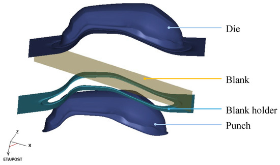
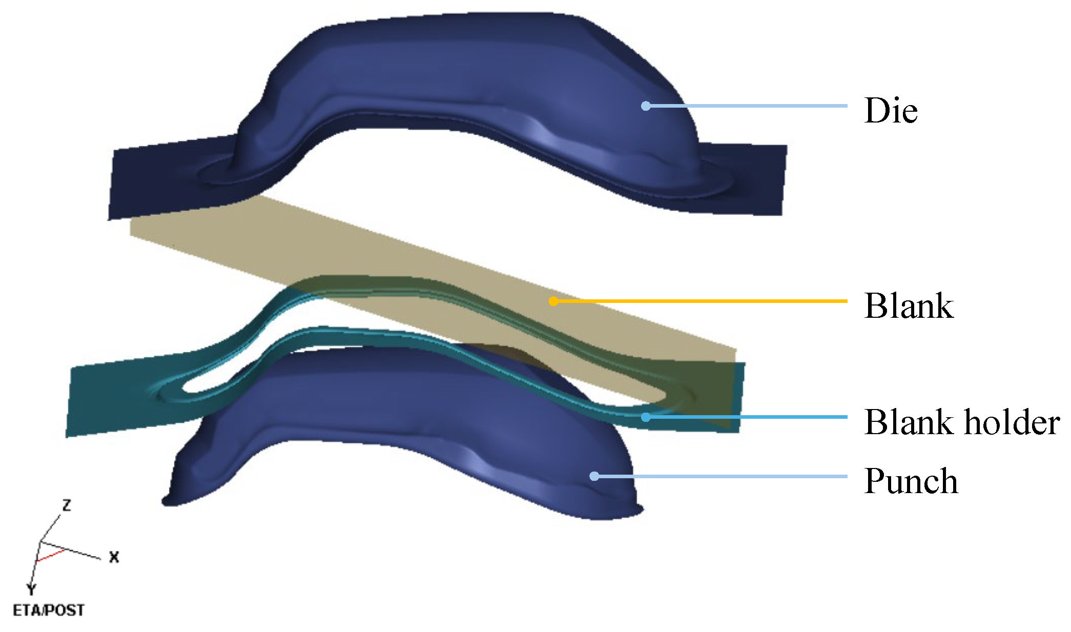
In the pre-processing stage, tool geometries were imported in the IGES format and modeled as rigid bodies, while a 740 × 510 mm² rectangular blank was defined as a deformable body. The relative positions of the tools and the blank for the deep drawing stage are illustrated in Figure 8.

Figure 8. Initial relative position of tools and blank for deep drawing simulation.

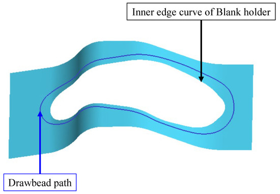
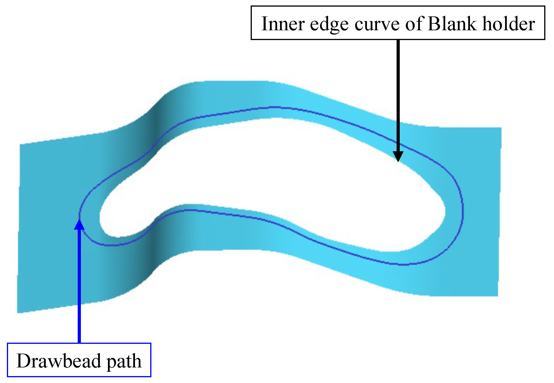
To facilitate the optimization process, the blank holder pressure and the drawbead geometries were assigned according to the experimental design detailed in Section 3.2.3 (Design of Experiments). Semi-circular drawbeads were generated using Dynaform’s geometric generation function. The drawbead path was defined by a 30 mm offset from the inner edge curve of the blank holder surface along the local tangential plane, as illustrated in Figure 9.

Figure 9. Drawbead path definition by offsetting the inner edge of the blank holder.

The deformable blank was meshed using Belytschko–Tsay elements with five integration points through the thickness. An initial mesh size of 16 mm was employed with four levels of adaptive refinement, allowing for a minimum element size of 1 mm for capturing high geometric gradients. For the material characterization of AA5754-O, the model incorporated an initial nominal thickness of 1.50 mm, a density of 2700 kg/m³, and a Poisson’s ratio of 0.33. The mechanical properties, constitutive models, and forming limits, as detailed in Section 2 (Studied Part and Material), were incorporated into the simulation setup.

4. Results and Discussion

A total of 20 simulation runs were conducted based on the inscribed central composite (CCI) experimental design detailed in Table 5. The resulting maximum thinning percentages (max. %Thinning) and the calculated Q-values are summarized in Table 6.

Table 6. Results of max. %Thinning and Q-value based on the inscribed central composite design.

Condition Number	Max. %Thinning [%]	Q-Value [-]
1	19.59	231.19
2	25.84	218.59
3	21.96	231.05
4	26.74	220.52
5	21.79	232.63
6	30.59	204.31
7	20.07	230.15
8	27.92	212.64
9	25.34	232.48
10	24.38	232.57
11	24.90	232.35
12	24.74	233.96
13	25.90	229.38
14	22.85	228.73
15	25.93	230.91
16	20.59	228.07
17	32.74	211.25
18	24.98	232.33
19	24.86	231.76
20	24.80	233.49

4.1. Repeatability Assessment of Results

The central composite experimental design includes replicated center points, facilitating the estimation of pure error to evaluate experimental repeatability. In this study, six center point runs (Condition Numbers 9–11 and 18–20) were conducted under identical conditions. To determine whether response variations were statistically significant relative to the effects of the input variables, F-tests for the max. %Thinning and Q-value were employed according to Equation (12), and the results are presented in Table 7 and Table 8, respectively.

$$\mathrm{F}-\mathrm{value}={\displaystyle \frac{\mathrm{Mean} \mathrm{Square} \mathrm{Error} \mathrm{of} \mathrm{Factorial} \mathrm{and} \mathrm{Axial} \mathrm{points}}{\mathrm{Mean} \mathrm{Square} \mathrm{Error} \mathrm{of} \mathrm{Center} \mathrm{points}}}$$

(12)

Table 7. F-test results for repeatability assessment of max. %Thinning.

	Center Points	Factorial and Axial Points
Degrees of Freedom	5	13
Mean	24.88	24.80
Total Sum of Squares	0.48	201.81
Mean Square Error	0.10	15.52
F-value	155.20

Table 8. F-test results for repeatability assessment of Q-value.

	Center Points	Factorial and Axial Points
Degrees of Freedom	5	13
Mean	232.50	224.53
Total Sum of Squares	1.58	1145.43
Mean Square Error	0.32	88.11
F-value	275.34

The F-test was conducted at a significance level of 0.05, corresponding to a 95% confidence level. The critical F-value (F_{0.05, 13, 5}) is 4.66. As shown in Table 7 and Table 8, the calculated F-values for both responses are substantially higher than this critical threshold. These results demonstrate that the experimental noise (pure error) is negligible compared to the variance induced by the changes in input variables. This confirms the high repeatability of the simulation and provides a reliable foundation for the subsequent analysis.

4.2. Response Surface Models

Regression analysis was utilized to model the relationships between input variables (BHP, H_{male bead}, and R_{female bead}) and the responses (max. %Thinning and Q-value). The three-variable full second-order response surface model was initially applied. Subsequently, model refinement was carried out using Bidirectional Stepwise Regression in MATLAB R2024b. The selection process was based on p-value thresholds of 0.05 for entry and 0.10 for removal to ensure that statistically significant terms were retained in the final response surface models.

The resulting regression coefficients and their corresponding p-values for both responses are summarized in Table 9 and Table 10, respectively.

Table 9. Regression coefficients of the refined response surface model for max. %Thinning.

Term	Coefficient Value	p-Value
Intercept	24.83	9.87 $\times$ 10−22
Hmale bead	1.01	0.05
Rfemale bead	0.50	0.31
BHP	5.93	6.04 $\times$ 10−9
Rfemale bead Hmale bead	−2.71	0.02
Hmale bead BHP	1.99	0.08

Table 10. Regression coefficients of the refined response surface model for Q-value.

Term	Coefficient Value	p-Value
Intercept	232.12	1.53 $\times$ 10−25
Hmale bead	−2.55	0.18
Rfemale bead	0.33	0.60 $\times$ 10−2
BHP	−13.27	5.20 $\times$ 10−9
Hmale bead BHP	−4.98	0.51 $\times$ 10−2
$R_{\mathit{female} \mathit{bead}}^2$	−3.13	0.76 $\times$ 10−2
BHP2	−18.98	1.96 $\times$ 10−8

Based on the regression coefficients in Table 9 and Table 10, the refined response surface models for max. %Thinning and Q-value are expressed in Equations (13) and (14) for coded units, and in Equations (15) and (16) for natural units, respectively.

max. %Thinning_{(coded unit)} = 24.83 + 1.01H_{male bead} + 0.50R_{female bead} + 5.93BHP − 2.71R_{female bead} H_{male bead} + 1.99H_{male bead} BHP

(13)

$$\mathrm{Q}-{\mathrm{value}}_{(\mathrm{coded} \mathrm{unit})}=232.12-2.55H_{\mathit{male} \mathit{bead}}+0.33R_{\mathit{female} \mathit{bead}}-13.27\mathit{BHP}-4.98H_{\mathit{male} \mathit{bead}} \mathit{BHP}-3.13R_{\mathit{female} \mathit{bead}}^2-{18.98\mathit{BHP}}^2$$

(14)

max. %Thinning = −3.97 + 2.82H_{male bead} + 3.83R_{female bead} − 0.24BHP − 1.07R_{female bead} H_{male bead} + 11.78H_{male bead} BHP

(15)

$$\mathrm{Q}-\mathrm{value}=34.84+11.00H_{\mathit{male} \mathit{bead}}+8.49R_{\mathit{female} \mathit{bead}}+770.20\mathit{BHP}-29.48H_{\mathit{male} \mathit{bead}} \mathit{BHP}-0.62R_{\mathit{female} \mathit{bead}}^2-{843.54\mathit{BHP}}^2$$

(16)

The fit statistics for max. %Thinning and Q-value refined response surface models are summarized in Table 11 to evaluate their robustness and monitor potential overfitting.

Table 11. Statistical model fit summary for the refined response surface models of max. %Thinning and Q-value.

Refined Model	R-Squared	Adjusted R-Squared	Predicted R-Squared
max. %Thinning	0.9239	0.8967	0.8053
Q-value	0.9691	0.9523	0.8404

Both models exhibit high R-squared and adjusted R-squared values. The small discrepancy between these metrics is well within the acceptable threshold of 0.2. These results were achieved by removing non-significant terms through stepwise regression, which reflects high accuracy and confirms that the refinement process did not lead to overfitting. Furthermore, the predicted R-squared values for both models exceed 0.8 and differ only slightly from the adjusted R-squared values, staying within the recognized 0.2 threshold. Consequently, the models are considered statistically robust for predicting formability within the design space.

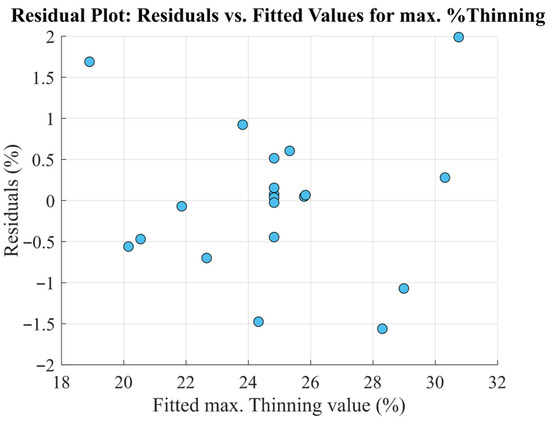
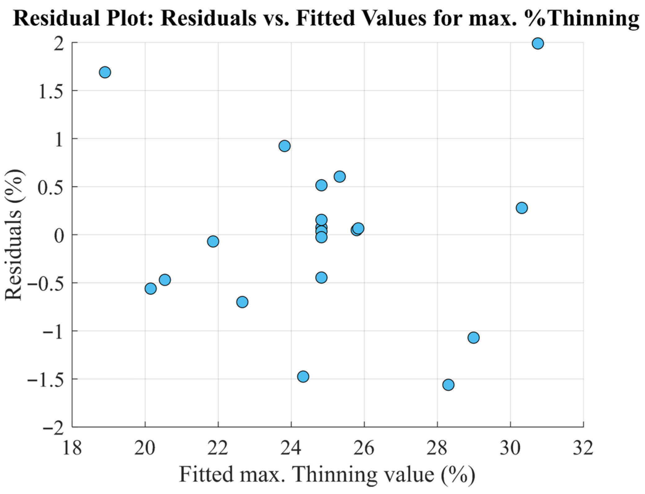
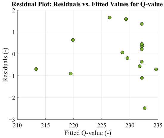
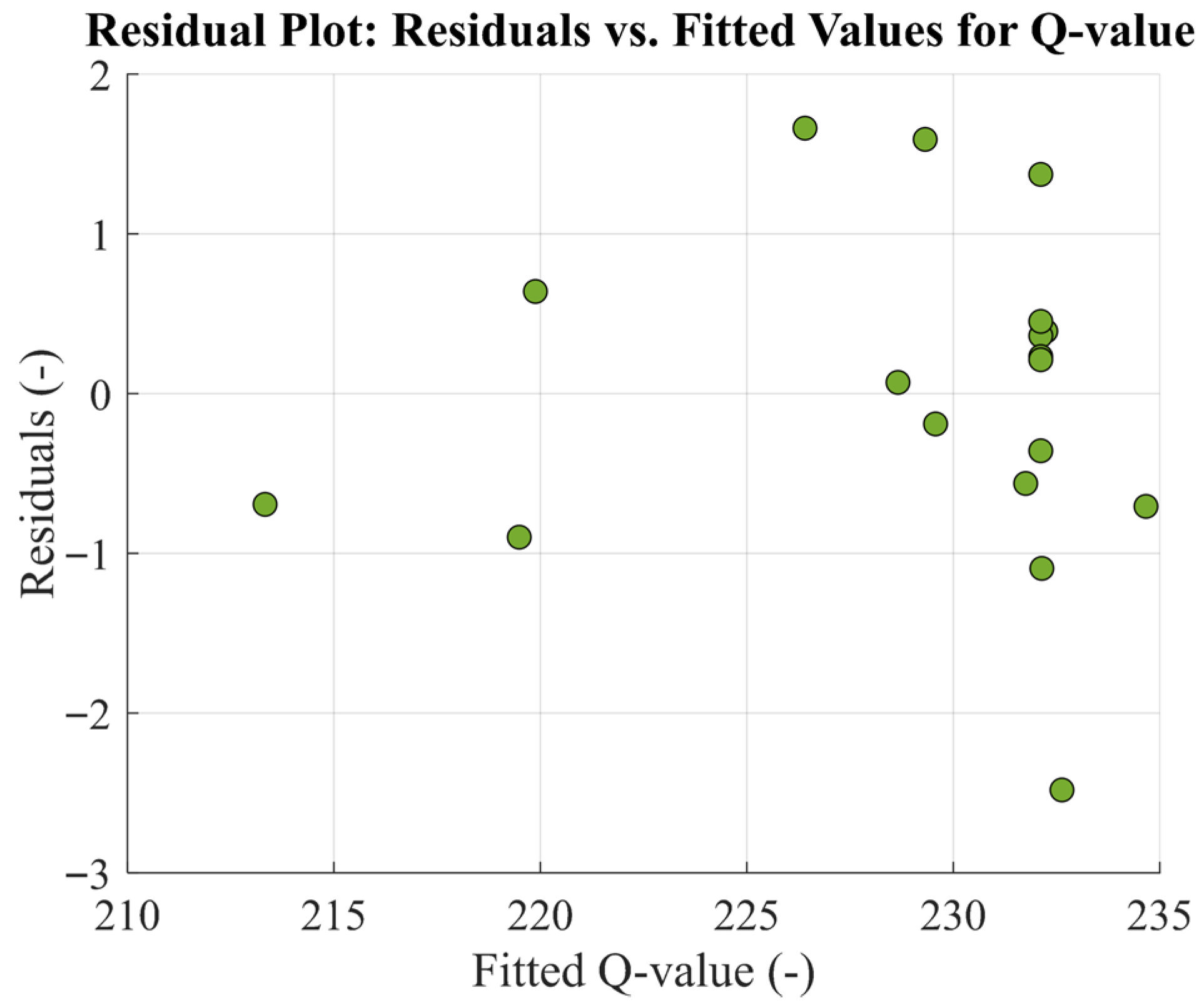
The normality of the residual distribution for the max. %Thinning and Q-value models were confirmed by skewness values of 0.36 and −0.37, respectively. These values fall within the generally accepted range of ±1. The residual plots in Figure 10 and Figure 11 exhibit random distributions without discernible patterns, indicating that the models effectively capture the systematic variation in the collected data.

Figure 10. Residual plot for the max. %Thinning response surface model.

Figure 11. Residual plots for the Q-value response surface model.

4.3. Parametric Analysis of Variable Effects on Max. %Thinning and Q-Value

The sensitivity of the responses to variable variations was investigated through the coded-unit response surface models. Each regression coefficient in the model represents the estimated change in the response resulting from a one-unit change in the corresponding term, with all other terms held constant. While the model coefficients provide the statistical foundation for sensitivity analysis, three-dimensional response surfaces and contour plots are simultaneously utilized to visualize the complex relationships, particularly the interaction effects and the global trends of the responses within the design space.

4.3.1. Variable Effects on Max. %Thinning

The refined coded-unit response surface model in Equation (13) is formulated as a first-order model with interaction terms consisting of all studied variables. Analysis of the coefficients reveals that BHP is the most dominant parameter, with a positive coefficient of 5.93. This magnitude is more than double that of the R_{female bead} H_{male bead} interaction term, which is the second most significant factor. This identifies BHP as the primary driver of max. %Thinning. The positive sign indicates a direct relationship, where increasing the BHP value within the investigated range leads to higher thinning.

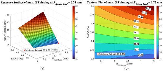
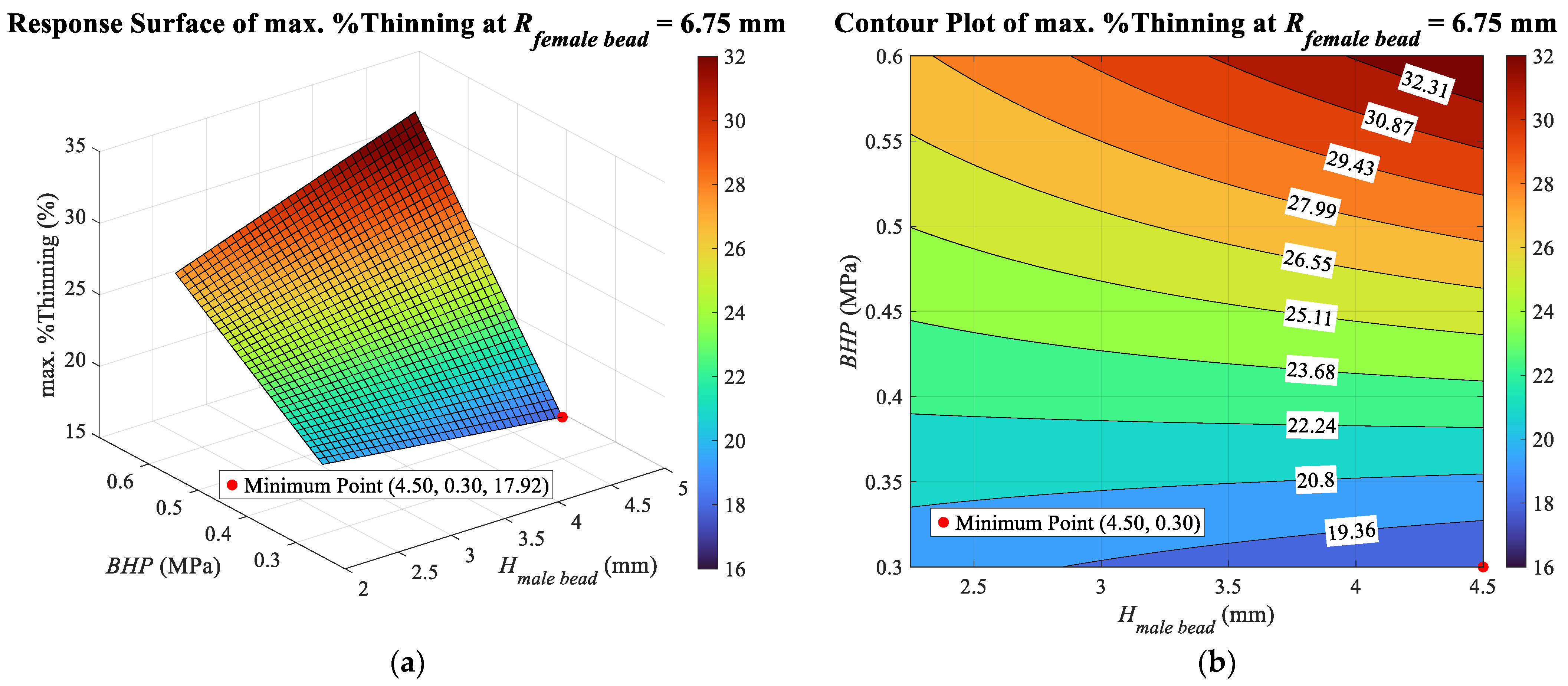
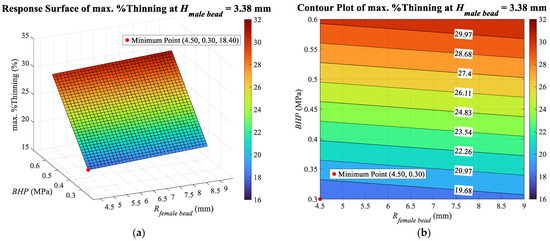
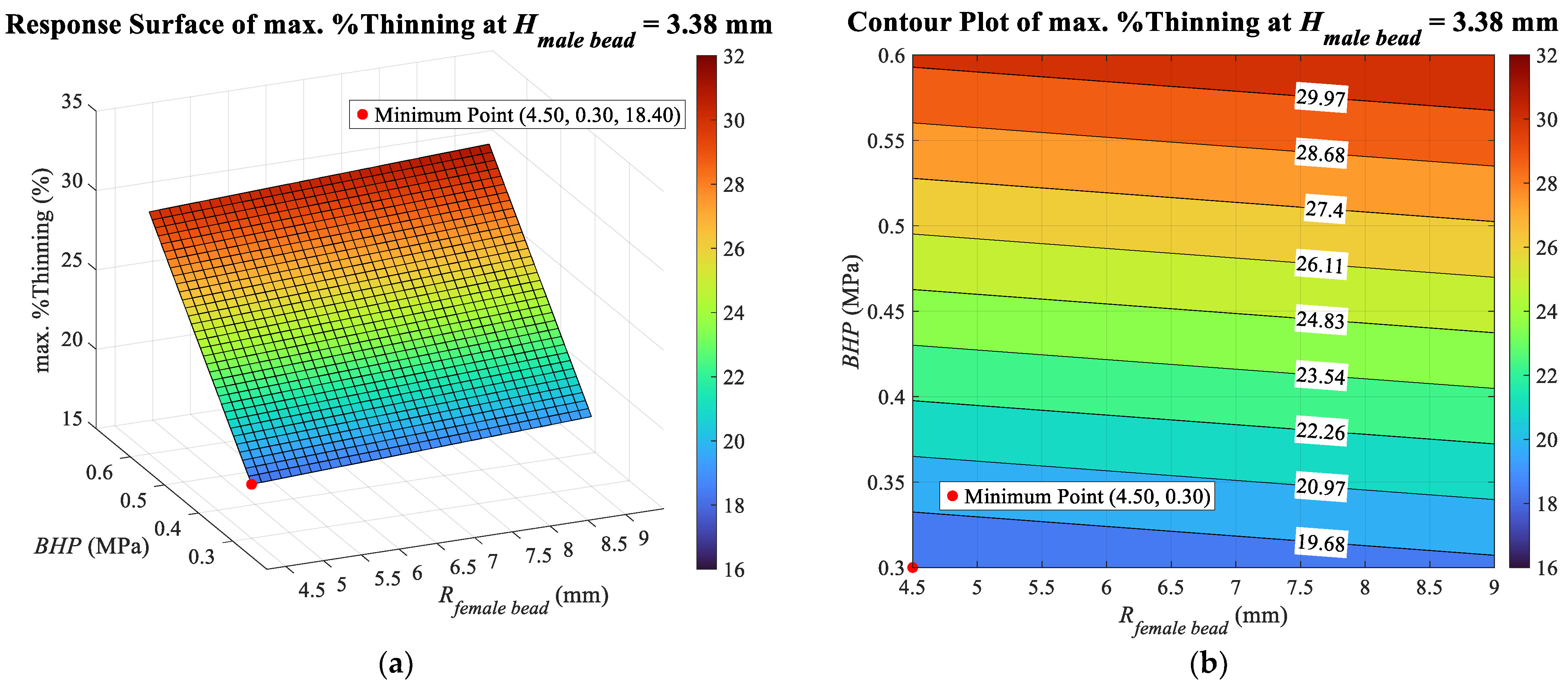
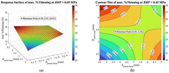
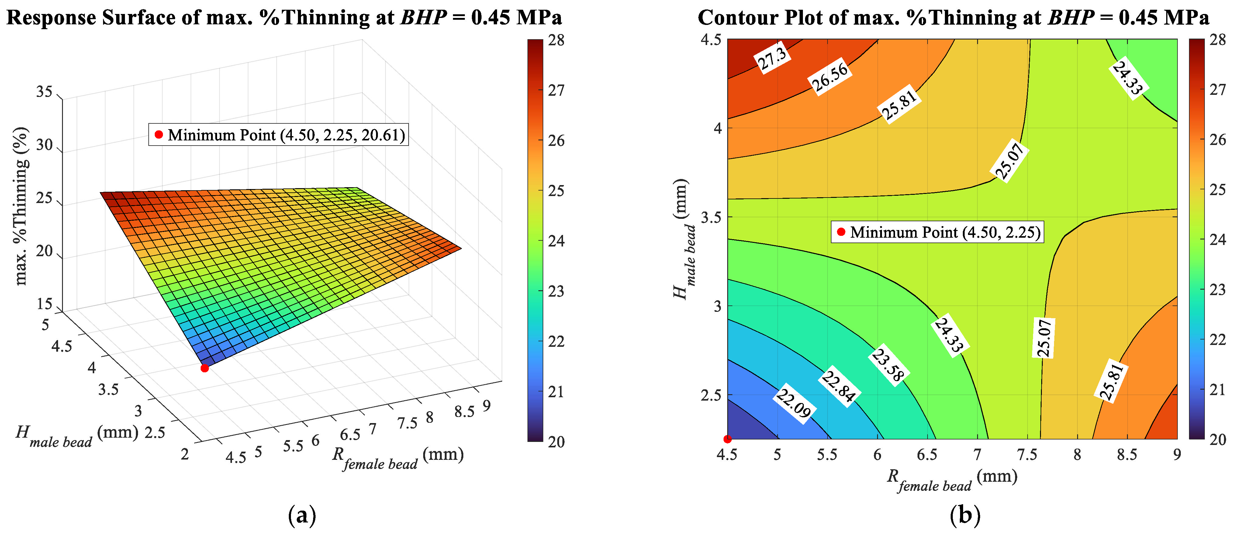
The response surfaces in Figure 12, Figure 13 and Figure 14 illustrate the interaction effects of the variables when one variable is held at its center point: R_{female bead} at 6.75 mm, H_{male bead} at 3.38 mm, and BHP at 0.45 MPa, respectively. The global trends in Figure 12 and Figure 13 confirm that the minimum thinning is consistently achieved with the lowest BHP. Additionally, the sensitivity of the max. %Thinning to BHP is evident when comparing Figure 12 and Figure 13 (where BHP varies) with Figure 14 (where BHP is constant). In the cases where BHP is a variable, the Z-axis (max. %Thinning) exhibits a significantly broader range.

Figure 12. Effect of H_{male bead} and BHP on max. %Thinning, with fixed R_{female bead} at 6.75 mm, shown in (a) response surface; (b) contour plot.

Figure 13. Effect of R_{female bead} and BHP on max. %Thinning, with fixed H_{male bead} at 3.38 mm, shown in (a) response surface; (b) contour plot.

Figure 14. Effect of R_{female bead} and H_{male bead} on max. %Thinning, with fixed BHP at 0.45 MPa, shown in (a) response surface; (b) contour plot.

An additional advantage of response surfaces is their ability to visualize complex interaction effects that may be overlooked when analyzing mathematical equations alone. For instance, while Equation (13) shows a positive coefficient of +1.01 for the H_{male bead}, which implies that increasing the male bead height exacerbates thinning, Figure 12a reveals a more nuanced behavior. Under a fixed R_{female bead} of 6.75 mm, the minimum thinning actually occurs at the highest male bead height. This demonstrates how response surfaces illustrate overall gradients to identify trends, while the corresponding contour plot (Figure 12b) provides the response-value identification required to navigate process windows and determine optimal parameters.

4.3.2. Variable Effects on Q-Value

The refined quadratic response surface model in Equation (14) incorporates all studied variables to characterize the Q-value response. Analysis of the regression coefficients reveals that the quadratic term of blank holder pressure (BHP²) and the linear term (BHP) are the most dominant parameters, with coefficients of 18.98 and 13.27, respectively. Notably, the next highest coefficient is the interaction term of H_{male bead} BHP, which is nearly three times smaller. The substantial gap emphasizes the dominance of blank holder pressure over the other two variables (H_{male bead} and R_{female bead}) within the investigated range.

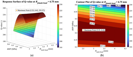
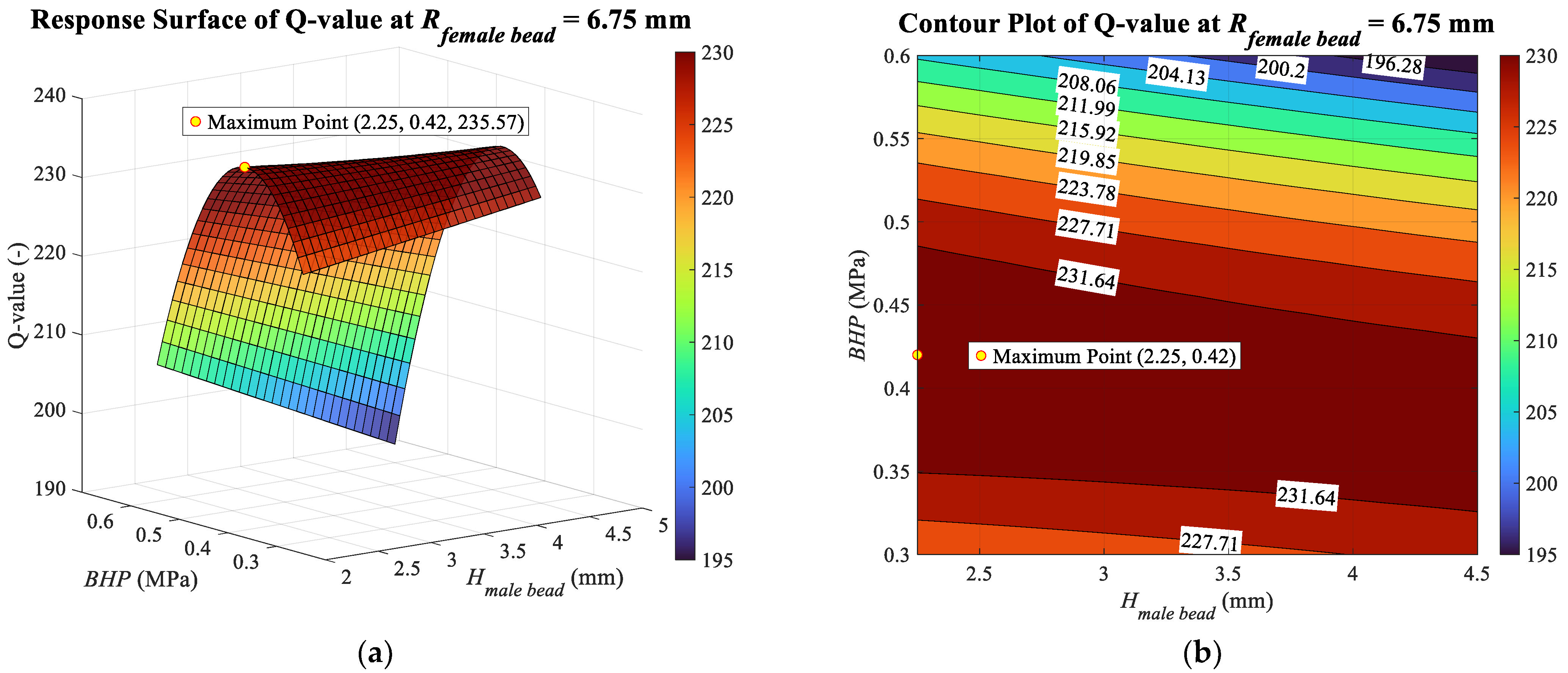
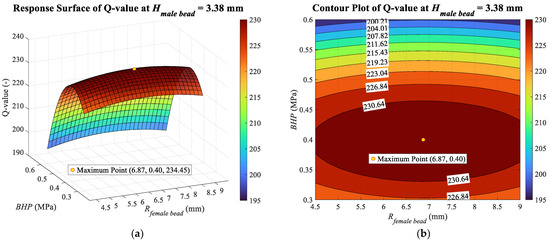
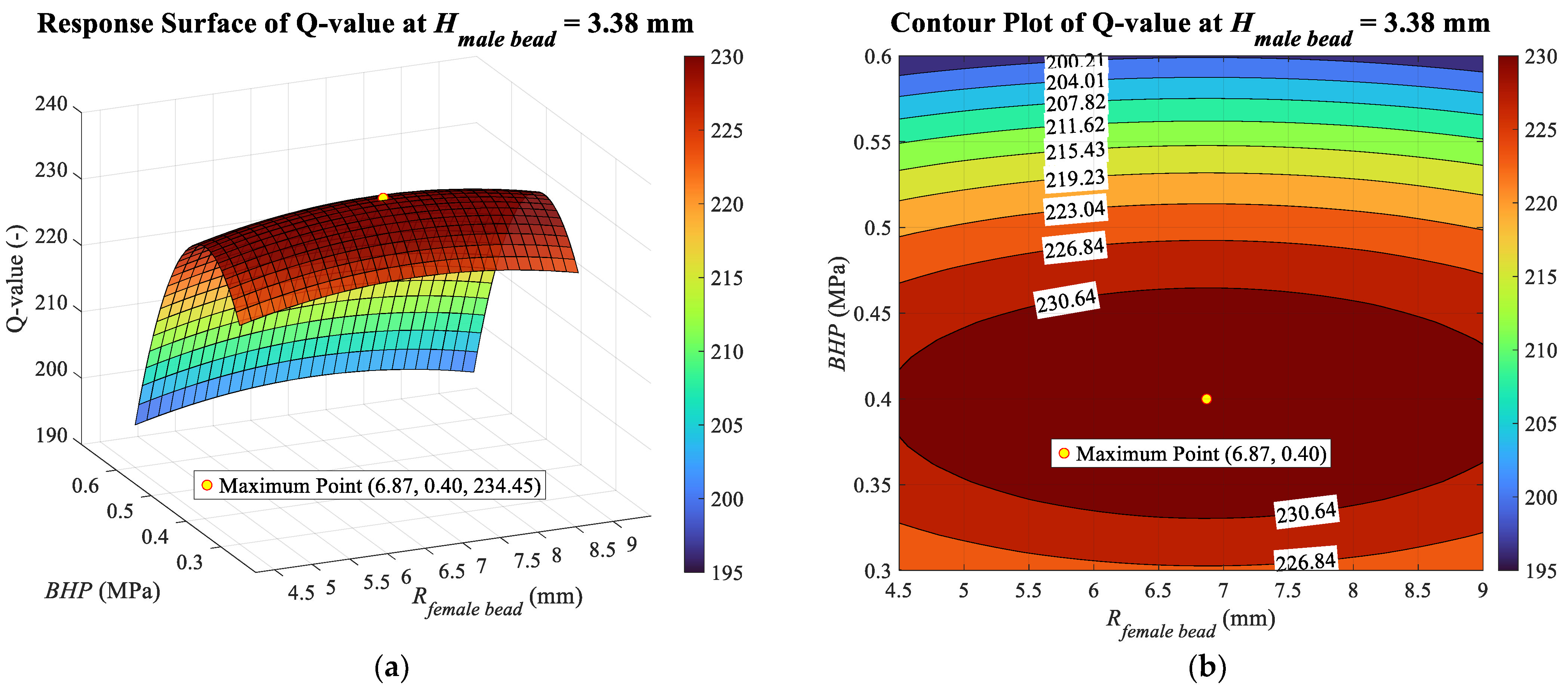
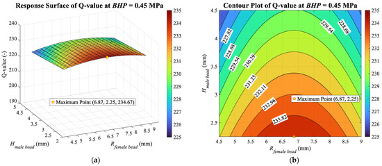
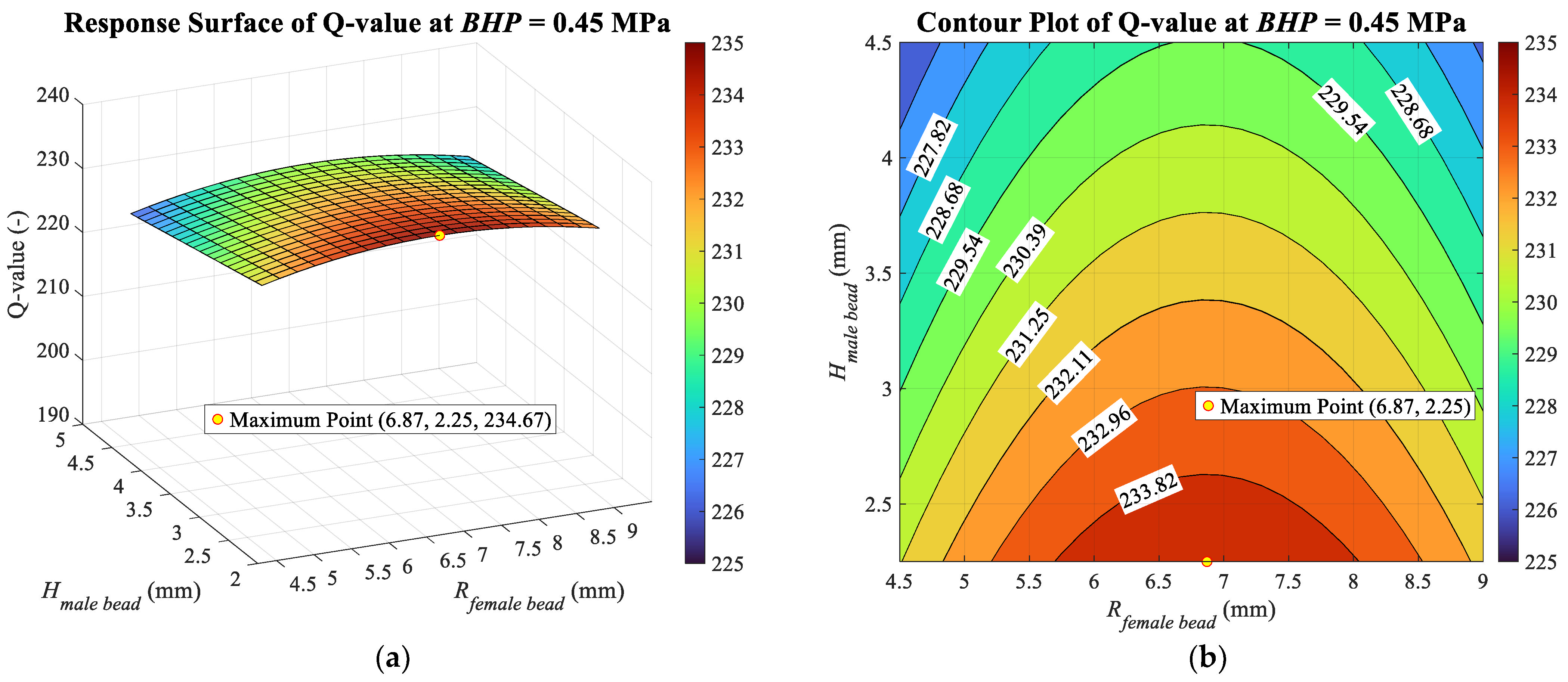
These findings identify blank holder pressure as the primary driver of Q-value, consistent with its observed dominant role in max. %Thinning. However, unlike the global linear trend observed in max. %Thinning response, the Q-value is characterized by non-linear behavior. In Figure 15 and Figure 16, where BHP is treated as a variable, the response surfaces exhibit a distinct peak. The downward-opening parabolic shape directly corresponds to the negative coefficient of the BHP² term.

Figure 15. Effect of H_{male bead} and BHP on Q-value, with fixed R_{female bead} at 6.75 mm, shown in (a) response surface; (b) contour plot.

Figure 16. Effect of R_{female bead} and BHP on Q-value, with fixed H_{male bead} at 3.38 mm, shown in (a) response surface; (b) contour plot.

Moreover, the negative sign of the second-order term for the female bead radius ($R_{\mathit{female} \mathit{bead}}^2$) results in a downward-opening parabolic trend, with the peak Q-value located near the center point of the investigated R_{female bead} range, as illustrated in Figure 16 and Figure 17.

Figure 17. Effect of R_{female bead} and H_{male bead} on Q-value, with fixed BHP at 0.45 MPa, shown in (a) response surface; (b) contour plot.

The diverging trends observed between the conditions for the minimum max. %Thinning and the maximum Q-value underscore the distinct optimization objectives associated with each response. A comparison between Figure 12 and Figure 15, in which BHP and H_{male bead} are treated as variables at a fixed R_{female bead} of 6.75 mm, reveals a discrepancy in the optimal conditions of the two variables. The Q-value reaches its peak near the center of the studied BHP range, at approximately 0.42 MPa, whereas max. %Thinning is minimized at the lowest BHP. Furthermore, while the Q-value is maximized at the lowest H_{male bead}, the max. %Thinning reaches its minimum at the highest H_{male bead} within the studied range.

A more robust comparison is evidenced in Figure 14 and Figure 17, where the drawbead geometries are varied at a constant BHP of 0.45 MPa. Although both the minimum max. %Thinning and the maximum Q-value are achieved at a consistent H_{male bead} of 2.25 mm, their required R_{female bead} values differ significantly. The minimum max. %Thinning requires the lowest investigated R_{female bead}, whereas the maximum Q-value requires a larger radius of 6.87 mm, located near the center of the studied range. These conflicting requirements confirm that each response prioritizes different aspects of formability, which are clearly captured within the studied variable ranges.

Consequently, individual optimizations for each response will be performed in the subsequent section based on the response surface models, followed by a comparative analysis of the results to clearly demonstrate the effectiveness of each approach.

4.4. Optimization of Variables for Individual Responses

To minimize the maximum percentage thinning and maximize the Q-value, the optimal conditions for the three studied variables (BHP, H_{male bead}, and R_{female bead}) were determined individually, based on the coded unit response surface models in Equations (13) and (14), respectively. The optimizations were executed using the ‘fmincon’ function in MATLAB R2024b, utilizing nonlinear optimization constrained by upper and lower bounds corresponding to the high and low levels of each investigated variable range. The optimized values in coded units were subsequently converted into natural units, as summarized in Table 12.

Table 12. Optimized variables for minimizing max. %Thinning and maximizing Q-value.

Response	BHP [MPa]	Hmale bead [mm]	Rfemale bead [mm]
max. %Thinning	0.31	2.82	4.69
Q-value	0.42	2.25	6.87

4.4.1. Results of Max. %Thinning-Based Optimization

Under the optimal conditions presented in Table 12, the response surface model predicts a minimum max. %Thinning of 17.84%. A simulation-based experiment was conducted using these optimized settings. The simulation yielded a max. %Thinning of 19.46%, which corresponds to an absolute error of 8.32% relative to the predicted value. Notably, this result demonstrates the lowest thinning compared to the initial twenty experimental runs.

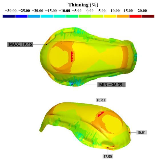
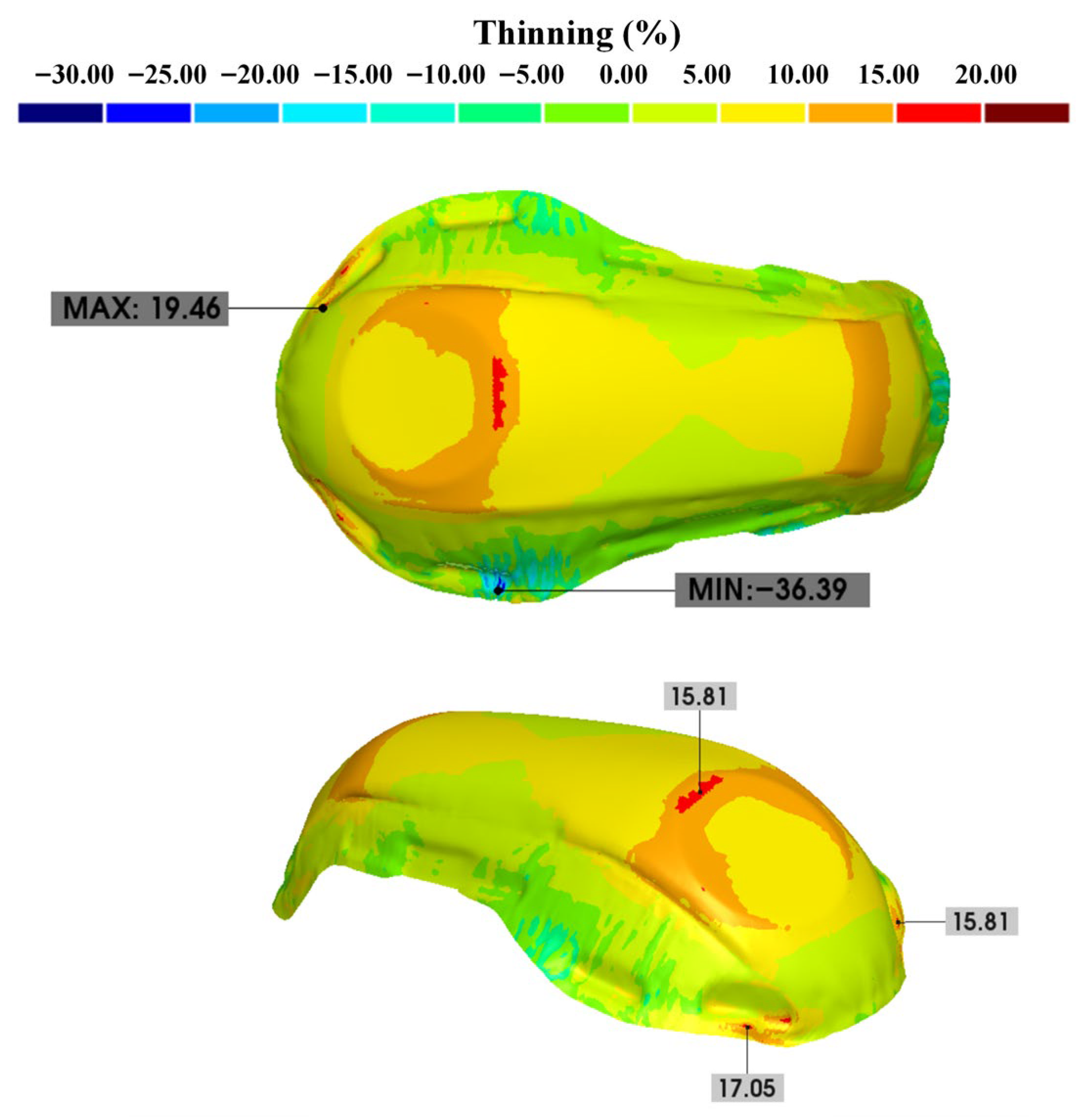
The distribution of thinning on the final flange-trimmed part under the optimal conditions is illustrated in Figure 18. Analysis of the distribution reveals that thinning is predominantly maintained within the 15% range, with only minimal areas exceeding this threshold. Similarly, thickening regions are primarily observed under 15%, with a peak thickening of 36.39%.

Figure 18. Thinning distribution of the flange-trimmed part formed under the optimal conditions for minimizing max. %Thinning.

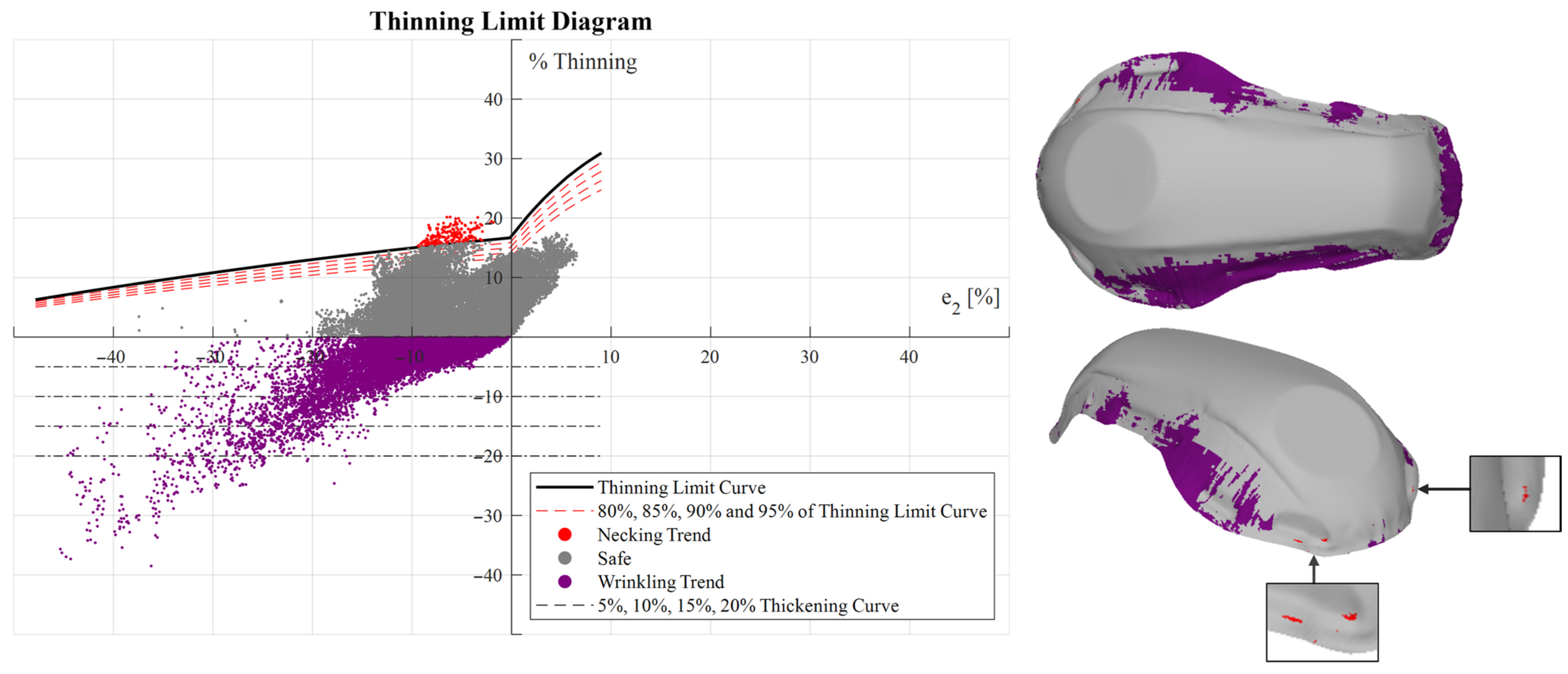
The Thinning Limit Diagram (TLD) obtained from the simulation results is illustrated in Figure 19, yielding a calculated Q-value of 227.98. Based on the red regions within the diagram, localized areas prone to necking are identified, as indicated by the rectangular highlights on the corresponding part. Additionally, regions with high material accumulation show a trend toward wrinkling (purple regions), which is consistent with the peak thickening values observed in the thinning distribution analysis.

Figure 19. Thinning Limit Diagram of the flange-trimmed part formed under the optimal conditions for minimizing max. %Thinning.

4.4.2. Results of Q-Value-Based Optimization

Under the optimized conditions summarized in Table 12, the response surface model predicts a maximum Q-value of 235.58. A simulation-based experiment was performed using these optimized settings, yielding a Q-value of 233.72. This represents an exceptionally low absolute error of only 0.80% relative to the predicted value.

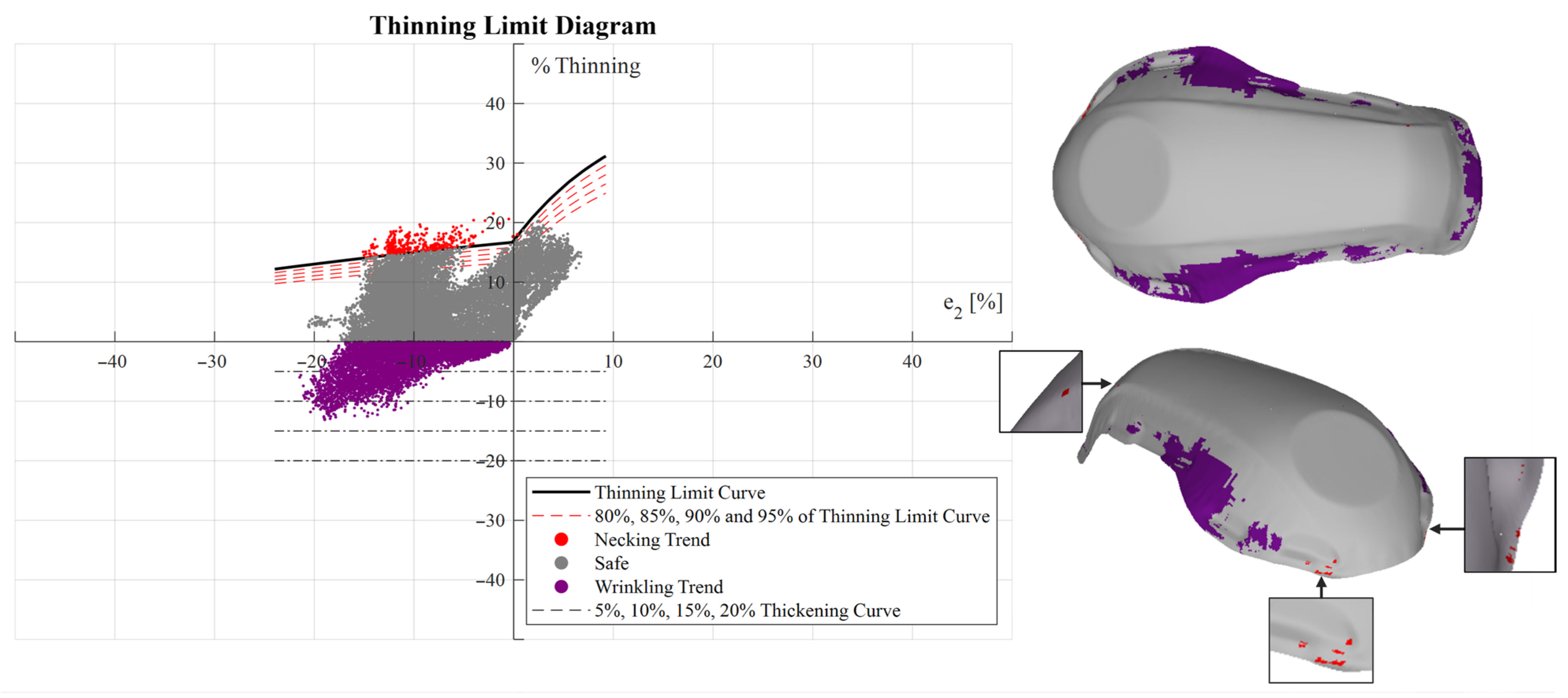
The Thinning Limit Diagram obtained from the simulation is presented in Figure 20. Compared with the optimized max. %Thinning case (Figure 19), this diagram shows a slightly larger red zone (necking trend) but a significantly smaller purple zone (wrinkling trend), especially in the side, head, and rear sections of the part. This analysis aligns with the thinning distribution illustrated in Figure 21.

Figure 20. Thinning Limit Diagram of the flange-trimmed part formed under the optimal conditions for maximizing Q-value.

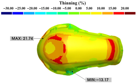
Figure 21. Thinning distribution of the flange-trimmed part formed under the optimal conditions for maximizing Q-value.

As shown in Figure 21, the maximum thinning is 21.74%, whereas the maximum thickening reaches 13.17%. In addition, thickening is commonly distributed within a 10% range, with only a limited zone exceeding this threshold at the peak thickening point. Remarkably, the thinning regions exceeding 15% are larger than those in the optimized max. %Thinning case, characterized by an expansion of the red color region (compared to Figure 18).

4.4.3. Comparison of Optimization Results

The comparison between the two optimization objectives reveals a critical trade-off in the forming performance of the AA5754-O part. While the objective of minimizing max. %Thinning (Section 4.4.1) achieved the lowest thinning value of 19.46%, it resulted in a peak thickening of 36.39%.

In contrast, the Q-value optimization (Section 4.4.2) offers the maximum thinning increase, marginally to 21.74%, and a dramatic decrease in maximum thickening to 13.17%. This represents a nearly threefold reduction in material accumulation compared to the optimized max. %Thinning case.

To provide a global assessment rather than focusing solely on localized peak values, the frequency distribution of elements across various severity levels was analyzed. This standardized comparison is necessary because the necking trend is not defined by a constant %Thinning value, as evidenced by the non-linear Thinning Limit Curve converted from the Forming Limit Curve.

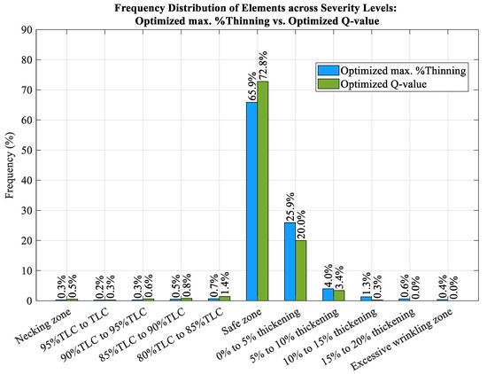
Consequently, the element count was normalized against the total number of elements to ensure a valid comparison between different cases. To establish a uniform basis for comparison, these elements were categorized using the same severity levels and 20% offset from both the Thinning Limit Curve (TLC) and the Wrinkling Limit Curve defined in the Q-value framework. The resulting frequency distributions for two optimization cases are illustrated in Figure 22.

Figure 22. Comparison of frequency distribution of normalized elements for max. %Thinning- and Q-value-optimized cases.

As illustrated in Figure 22, the necking trend severity levels (represented by the five bars on the left) for the optimized max. %Thinning case are slightly lower than those of the optimized Q-value case. The percentage of elements that exceed the TLC (necking zone) is minimal: lower than 1% for both cases, with the Q-value case being 0.2% higher. In the subsequent offset from the TLC zones, the element frequencies for the Q-value case are higher by 0.1%, 0.1%, 0.3%, 0.3%, and 0.7%, respectively. This confirms that direct optimization of max. %Thinning is more effective at specifically targeting thinning responses as a direct objective function.

The analysis of wrinkling trend (depicted by the five bars on the right) shows that the optimized Q-value outperforms the optimized max. %Thinning approach across all intervals. For the excessive wrinkling zone, the optimized Q-value case is successfully reduced to 0.0%, compared to 0.4% in the optimized max. %Thinning case. Across other thickening ranges (0% to 20%), the frequencies of the optimized Q-value case are lower by 5.9%, 0.6%, 1.0%, and 0.6%, respectively.

These results reflect a more balanced forming performance achieved by the Q-value approach. While this approach does not minimize thinning as aggressively as direct optimization (max. %Thinning-based optimization), the resulting differences in thinning behavior are marginal. In contrast, the improvement in the wrinkling approach is observed. A mechanical analysis of blank holder pressure (BHP), the most influential variable for both objective functions, clarifies these results. A lower BHP helps relieve thinning but neglects wrinkling risks, as evidenced by the max. % Thinning optimization results in Section 4.4.1. However, the Q-value index effectively accounts for the second-order influence of BHP. This influence exhibits a characteristic peak, signifying the optimal balance between excessive thinning (dominant at high pressures) and dominant wrinkling (caused by insufficient pressure). This finding is consistent with established research investigating the critical influence of blank holder loads on material formability [78,79]. Ultimately, the Q-value optimization leads to a significantly higher safe zone occupancy of 72.8%, compared to 65.9% in the max. %Thinning case. This global analysis confirms that maximizing the Q-value ensures the overall integrity of the component by effectively managing the trade-off between risk of necking and wrinkling failures for the studied complex automotive part.

5. Experimental Validation of the Part Formed Under the Optimized Q-Value

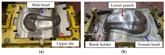
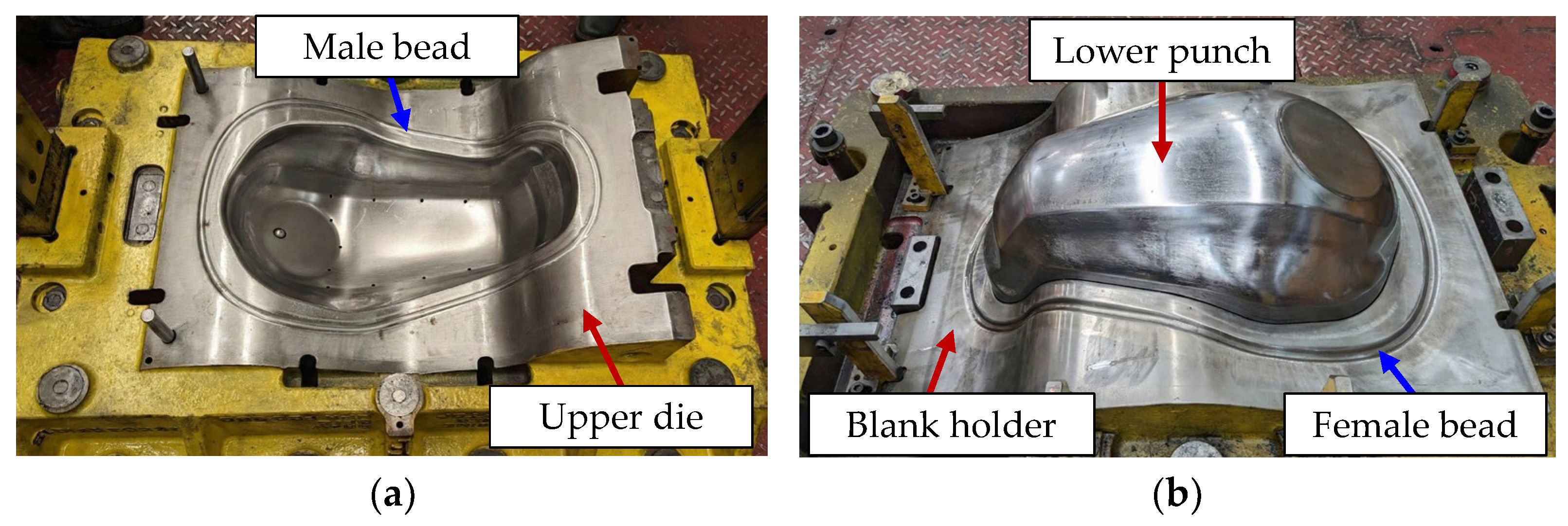
The shape and thickness of the experimentally formed part were examined under the optimized Q-value condition to validate the accuracy of the numerical simulations and the reliability of the optimization results. To maintain consistency with the simulation parameters, lubricating oil was applied uniformly to the aluminum blank surfaces using a paint roller prior to the forming operation. The blank is firstly formed using a 1000-ton single-action hydraulic press with a die cushion for the primary deep drawing stage. The upper and lower tools corresponding to the optimized drawbead geometry, which were equipped on the press, are shown in Figure 23. Following minor-sunken stamping by a 600-ton double crank mechanical press, 3D-laser trimming was performed, resulting in the final geometry.

Figure 23. Physical deep drawing tools: (a) upper tool; (b) lower tool.

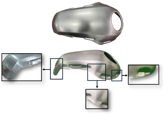
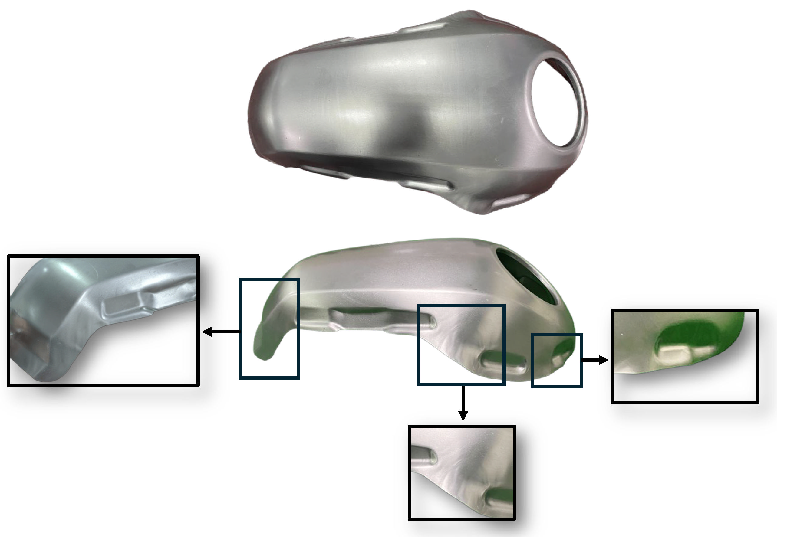
The resulting physical component is illustrated in Figure 24. A comparison of the wrinkling regions between the physical component and the simulation results in Figure 20 demonstrates a strong correlation. The predicted wrinkling patterns are indicated by the purple regions in the simulation. These patterns align precisely with the actual wrinkles observed on the experimental part, as shown in the magnified views within Figure 24. This close agreement further validates the ability of the finite element model to predict localized surface wrinkling behavior accurately.

Figure 24. The physical part formed under the optimized Q-value condition.

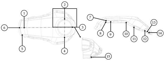
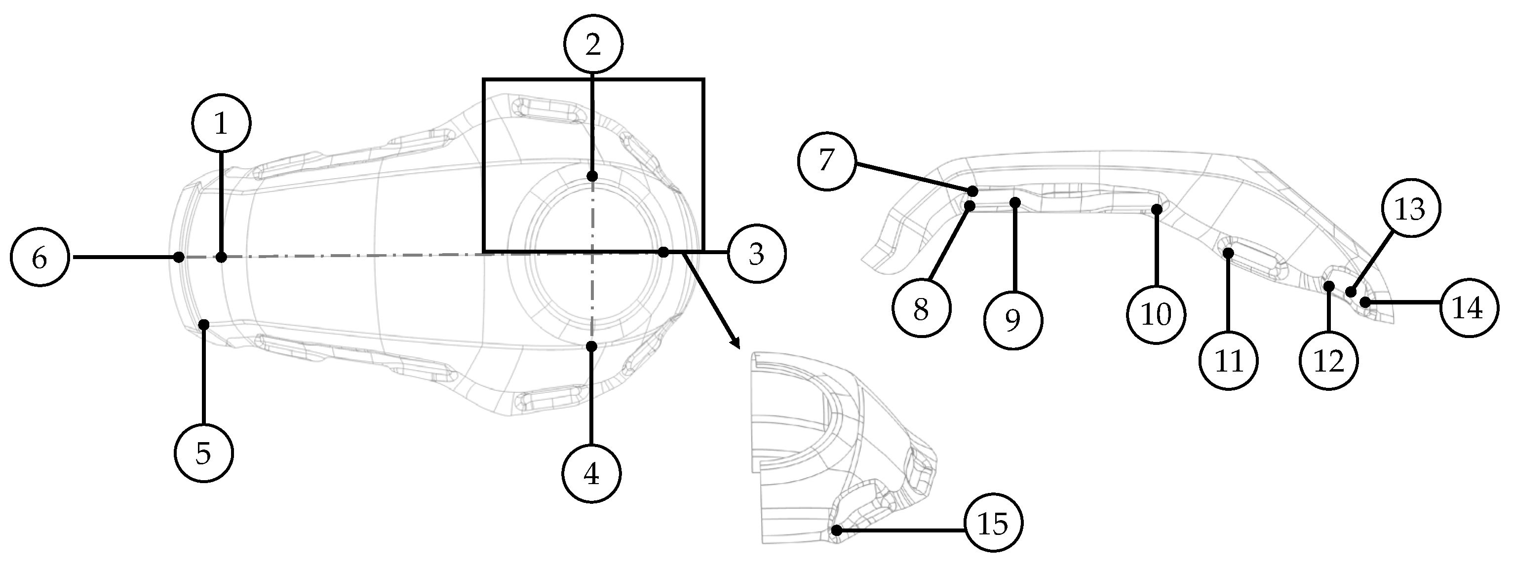
Non-destructive thickness measurements were performed to evaluate thinning behavior. Critical areas prone to thinning, such as the sunken and edge regions, were assessed using an Ultrasonic thickness gauge (resolution 0.01 mm, Dakota Ultrasonics PVX model). A total of fifteen measurement points were identified, as shown in Figure 25, and the comparison between these experimental measurements and the simulated results is summarized in Table 13.

Figure 25. Identification of 15 thickness measurement points for experimental validation.

Table 13. Comparison of simulated and experimentally measured thickness at fifteen locations on the Q-value optimized part.

Position (Point)	Thickness [mm]		Absolute Error [%]
	Simulated	Experimental
1	1.28	1.31	2.29
2	1.28	1.30	1.54
3	1.34	1.30	3.08
4	1.31	1.33	1.50
5	1.40	1.42	1.41
6	1.48	1.51	1.99
7	1.43	1.43	0.00
8	1.45	1.46	0.68
9	1.46	1.53	4.58
10	1.45	1.46	0.68
11	1.42	1.49	4.70
12	1.30	1.39	6.47
13	1.32	1.36	2.94
14	1.17	1.15	1.74
15	1.25	1.15	8.70

The results of the thickness validation indicate that the simulation is in acceptable close agreement with the experimental data, with the maximum deviation of 8.70% observed at point 15. Moreover, the simulation identified point 14 as the location of minimum thickness, which corresponds precisely with the experimental findings. The deviation between the simulated and measured values at this critical point was only 1.74%. Furthermore, the necking zone identified by the Thinning Limit Diagram, highlighted in the red region of Figure 20, aligned with points 14 and 15, where significantly higher thinning was observed compared to other regions. This consistency indicates a strong correlation between the simulation and experimental results, confirming the necking tendency predicted by the diagram.

6. Conclusions

This study compares the optimization results of the deep drawing process for a complex automotive component using two objective functions: the Q-value and the conventional maximum percentage of thinning (max. %Thinning). The main conclusions are summarized as follows:

• Response surface methodology (RSM) was successfully developed to refine second-order response surface models for both objective functions. Both max. %Thinning and Q-value responses achieved high statistical significance with R-squared values exceeding 80%. The absence of overfitting was verified through the analysis of adjusted and predicted R-squared values. The predictive capability of the models was further confirmed by low absolute errors of 8.32% for the optimized max. %Thinning and a remarkable 0.8% for the optimized Q-value. These results prove that the models maintain high accuracy even for coordinates outside the initial input data space. Furthermore, the manufacturing process window demonstrated the global influence of the studied variables (blank holder pressure, height of male bead, and radius of female bead) on both objective functions observed through response surfaces and contour plots.
• Parametric influence: All three studied variables within the investigated ranges significantly influenced the responses. Notably, blank holder pressure was identified as the most influential variable for both max. %Thinning and Q-value.
• The investigated parameter space revealed a clear trade-off between necking and wrinkling occurring in the optimized max. %Thinning case. In contrast, the Q-value-based optimization proved more effective in managing the critical trade-off. This is evidenced by the local maximum thinning and maximum thickening observed in the simulated parts. For the optimized Q-value condition, the maximum thinning and thickening were 21.74% and 13.17%, respectively, whereas for the optimized max. %Thinning condition, the corresponding values were 19.46% and 36.39%. In addition, the global proportion of elements in the “Safe Zone” of the Thinning Limit Diagrams (TLD) for the Q-value condition was 72.8%, compared to 65.9% for the max. %Thinning condition.

It is important to emphasize that Q-value optimization is not intended to replace the conventional maximum thinning assessment. Direct optimization of max. %Thinning remains effective for achieving its specific objective, yielding a minimum thinning value in this study. Rather, the Q-value serves as an extended quantitative formability tool that complements conventional approaches, particularly in manufacturing scenarios where balanced formability is required to ensure the overall formation of the part, rather than focusing solely on a localized indicator such as maximum thinning.

For future work, the proposed framework can be extended to incorporate additional process parameters, enabling improved generalizability of the Q-value and more rigorous validation of its effectiveness across diverse and complex forming conditions, thereby enhancing its potential for industrial applications.

References

- El Sherbiny, M.; Zein, H.; Abd-Rabou, M. Thinning and Residual Stresses of Sheet Metal in the Deep Drawing Process. Mater. Des. 2014, 55, 869–879. [Google Scholar] [CrossRef] [Scilit]
- Zein, H.; El Sherbiny, M.; Abd-Rabou, M. Thinning and Spring Back Prediction of Sheet Metal in the Deep Drawing Process. Mater. Des. 2014, 53, 797–808. [Google Scholar] [CrossRef] [Scilit]
- Lei, C.; Mao, J.; Zhang, X.; Wang, L.; Chen, D. Crack Prediction in Sheet Forming of Zirconium Alloys Used in Nuclear Fuel Assembly by Support Vector Machine Method. Energy Rep. 2021, 7, 5922–5932. [Google Scholar] [CrossRef] [Scilit]
- Kim, J.J.; Pham, Q.T.; Kim, Y.S. Thinning Prediction of Hole-Expansion Test for DP980 Sheet Based on a Non-Associated Flow Rule. Int. J. Mech. Sci. 2021, 191, 106067. [Google Scholar] [CrossRef] [Scilit]
- Hashemi, S.J.; Roohi, A.H. Minimizing Spring-Back and Thinning in Deep Drawing Process of St14 Steel Sheets. Int. J. Interact. Des. Manuf. (IJIDeM) 2022, 16, 381–388. [Google Scholar] [CrossRef] [Scilit]
- Modanloo, V.; Akhoundi, B.; Khatir, F.A.; Talebi-Ghadikolaee, H.; Mashayekhi, A. Investigation of the Effect of Process Parameters in Sheet Hydroforming Process. Int. J. Interact. Des. Manuf. (IJIDeM) 2023, 17, 3189–3198. [Google Scholar] [CrossRef] [Scilit]
- Thi, T.N.; Quang, N.H.; Thuy, M.T.; Duong, N.H. Research on Thinning Variation of the Copper Upper Sheet in Copper-Steel Double-Sheet Hydroforming. In Proceedings of the 2024 IEEE 11th International Conference on Computational Cybernetics and Cyber-Medical Systems (ICCC), Hanoi, Vietnam, 4–6 April 2024; IEEE: New York, NY, USA, 2024; pp. 321–326. [Google Scholar]
- Taşkın, A.; Dengiz, C.G. Experimental and Numerical Optimization of Deep Drawing Process Parameters for Square Medical Container Design with the Taguchi Method. Int. J. Adv. Manuf. Technol. 2024, 132, 2643–2659. [Google Scholar] [CrossRef] [Scilit]
- Leelaseat, J.; Larpprasoetkun, P.; Sunanta, A.; Nakwattanaset, A.; Suranuntchai, S. Investigation on the Effect of Blank Holder Force and Initial Blank Size on the Thinning Problem of the Fuel Tank Part Made from Aluminum Alloy Sheet 5754-O under Deep Drawing Process. Key Eng. Mater. 2024, 973, 101–107. [Google Scholar] [CrossRef] [Scilit]
- Kakandikar, G.M.; Nandedkar, V.M. Prediction and Optimization of Thinning in Automotive Sealing Cover Using Genetic Algorithm. J. Comput. Des. Eng. 2016, 3, 63–70. [Google Scholar] [CrossRef] [Scilit]
- Guo, Y.Q.; Batoz, J.L.; Naceur, H.; Bouabdallah, S.; Mercier, F.; Barlet, O. Recent Developments on the Analysis and Optimum Design of Sheet Metal Forming Parts Using a Simplified Inverse Approach. Comput. Struct. 2000, 78, 133–148. [Google Scholar] [CrossRef] [Scilit]
- Jakumeit, J.; Herdy, M.; Nitsche, M. Parameter Optimization of the Sheet Metal Forming Process Using an Iterative Parallel Kriging Algorithm. Struct. Multidiscip. Optim. 2005, 29, 498–507. [Google Scholar] [CrossRef] [Scilit]
- Kahhal, P.; Brooghani, S.Y.A.; Azodi, H.D. Multi-Objective Optimization of Sheet Metal Forming Die Using Genetic Algorithm Coupled with RSM and FEA. J. Fail. Anal. Prev. 2013, 13, 771–778. [Google Scholar] [CrossRef] [Scilit]
- Leelaseat, J.; Sunanta, A.; Suranuntchai, S. Formability Assessment Based on Q-Value for Optimizing the Deep Drawing Process of Automotive Parts Made from Aluminum Alloys Sheet. Metals 2025, 15, 68. [Google Scholar] [CrossRef] [Scilit]
- Merkani, M.S.; Parvizi, A. Optimization of Deep Drawing Products by Adding Effect of Texture Pattern in Draw Bead Design. J. Braz. Soc. Mech. Sci. Eng. 2022, 44, 1–16. [Google Scholar] [CrossRef] [Scilit]
- Semman, M.M.; Shazly, M.; Gadallah, M.H.; Mohamed, T.A.; Wifi, A.S. Prediction of Defects in Deep Drawn Rectangular Parts Using Finite Element Analysis (FEA) and Response Surface Methodology (RSM). J. Phys. Conf. Ser. 2024, 2811, 012013. [Google Scholar] [CrossRef] [Scilit]
- Singh Sivam, S.P.S.; Rajendran, R.; Harshavardhana, N. An Investigation of Hybrid Models FEA Coupled with AHP-ELECTRE, RSM-GA, and ANN-GA into the Process Parameter Optimization of High-Quality Deep-Drawn Cylindrical Copper Cups. Mech. Based Des. Struct. Mach. 2024, 52, 498–522. [Google Scholar] [CrossRef] [Scilit]
- Celik, I.; Şensoy, A.T.; Seven, G.; Cicek, D. Improving Deep Drawing Quality of DD13 Sheet Metal: Optimization of Process Parameters Using Box–Behnken Design. Materials 2025, 18, 1424. [Google Scholar] [CrossRef] [Scilit]
- Montgomery, D.C. Design and Analysis of Experiments; John Wiley & Sons, Inc.: New York, NY, USA, 2013; ISBN 9781118146927. [Google Scholar]
- Jivan, R.B.; Eskandarzade, M.; Bewsher, S.R.; Leighton, M.; Mohammadpour, M.; Saremi-Yarahmadi, S. Application of Solid Lubricant for Enhanced Frictional Efficiency of Deep Drawing Process. Proc. Inst. Mech. Eng. C J. Mech. Eng. Sci. 2022, 236, 624–634. [Google Scholar] [CrossRef] [Scilit]
- Gao, Y.; Li, H.; Zhao, D.; Wang, M.; Fan, X. Advances in Friction of Aluminium Alloy Deep Drawing. Friction 2024, 12, 396–427. [Google Scholar] [CrossRef] [Scilit]
- Takalkar, A.S.; Chinnapandi, L.B.M. Deep Drawing Process at the Elevated Temperature: A Critical Review and Future Research Directions. CIRP J. Manuf. Sci. Technol. 2019, 27, 56–67. [Google Scholar] [CrossRef] [Scilit]
- Dong, F.; Huang, S.; Yi, Y.; He, H.; Huang, K.; Wang, C.; Gao, S.; Jia, Y.; Yu, W. Enhanced Deep Drawing Formability and Deformation Mechanism of Aluminum Alloy at Cryogenic Temperature. J. Alloys Compd. 2023, 968, 171992. [Google Scholar] [CrossRef] [Scilit]
- Regueras, J.M.G.; López, A.M.C. Investigations on the Influence of Blank Thickness (t) and Length/Wide Punch Ratio (LD) in Rectangular Deep Drawing of Dual-Phase Steels. Comput. Mater. Sci. 2014, 91, 134–145. [Google Scholar] [CrossRef] [Scilit]
- Pitkin, N.; Uzun, U.; Knezevic, M. Improving R-Value of AA6016 Sheets by Cyclic-Bending-under-Tension and Heat-Treating Processes. J. Manuf. Process. 2025, 154, 623–639. [Google Scholar] [CrossRef] [Scilit]
- Xu, S.G.; Bohn, M.L.; Weinmann, K.J. Drawbeads in Sheet Metal Stamping—A Review. In Proceedings of the International Congress & Exposition, Detroit, MI, USA, 24 February 1997. [Google Scholar]
- Phanitwong, W.; Thipprakmas, S. Analysis of Draw Bead Geometry on Wall Thinning and Concave/Convex Feature in Rectangular Deep Drawn Parts. Adv. Mater. Res. 2011, 189–193, 2704–2707. [Google Scholar] [CrossRef] [Scilit]
- Ke, J.; Liu, Y.; Zhu, H.; Zhang, Z. Formability of Sheet Metal Flowing through Drawbead—An Experimental Investigation. J. Mater. Process. Technol. 2018, 254, 283–293. [Google Scholar] [CrossRef] [Scilit]
- Bassoli, E.; Sola, A.; Denti, L.; Gatto, A. Experimental Approach to Measure the Restraining Force in Deep Drawing by Means of a Versatile Draw Bead Simulator. Mater. Manuf. Process. 2019, 34, 1286–1295. [Google Scholar] [CrossRef] [Scilit]
- Wei, Z.; Zhang, Z.L.; Dong, X.H. Deep Drawing of Rectangle Parts Using Variable Blank Holder Force. Int. J. Adv. Manuf. Technol. 2006, 29, 885–889. [Google Scholar] [CrossRef] [Scilit]
- Candra, S.; Batan, I.M.L.; Berata, W.; Pramono, A.S. Modeling of the Minimum Variable Blank Holder Force Based on Forming Limit Diagram (FLD) in Deep Drawing Process. IOP Conf. Ser. Mater. Sci. Eng. 2017, 273, 012014. [Google Scholar] [CrossRef]
- Liu, Z.-Y.; Xiong, B.-Q.; Li, X.-W.; Yan, L.-Z.; Li, Z.-H.; Zhang, Y.-A.; Liu, H.-W. Deep Drawing of 6A16 Aluminum Alloy for Automobile Body with Various Blank-Holder Forces. Rare Met. 2019, 38, 946–953. [Google Scholar] [CrossRef] [Scilit]
- Mulyanto, B.; Khaerudini, D.S. Simulation and experimental investigation of wrinkle defect in deep drawing process of carbon steel spcc shaped cylinder flange cup. SINERGI 2020, 24, 197. [Google Scholar] [CrossRef] [Scilit]
- Asgharpour, A.; Gorji, H.; Delpazir, S.E. Experimental and Numerical Investigation to Determine the Optimal Blank-Holder Force in Deep Drawing Process Based on Forming Force for SS304L and St14 Sheets. J. Braz. Soc. Mech. Sci. Eng. 2024, 46, 349. [Google Scholar] [CrossRef] [Scilit]
- Tisza, M.; Czinege, I. Comparative Study of the Application of Steels and Aluminium in Lightweight Production of Automotive Parts. Int. J. Lightweight Mater. Manuf. 2018, 1, 229–238. [Google Scholar] [CrossRef] [Scilit]
- Varshney, D.; Kumar, K. Application and Use of Different Aluminium Alloys with Respect to Workability, Strength and Welding Parameter Optimization. Ain Shams Eng. J. 2021, 12, 1143–1152. [Google Scholar] [CrossRef] [Scilit]
- Davis, J.R. Alloying: Understanding the Basics; ASM International: Almere, The Netherlands, 2001; ISBN 1615030638. [Google Scholar]
- Sarkar, J.; Kutty, T.R.G.; Conlon, K.T.; Wilkinson, D.S.; Embury, J.D.; Lloyd, D.J. Tensile and Bending Properties of AA5754 Aluminum Alloys. Mater. Sci. Eng. A 2001, 316, 52–59. [Google Scholar] [CrossRef] [Scilit]
- ASTM E8/E8M-16a; Standard Test Methods for Tension Testing of Metallic Materials. ASTM International: West Conshohocken, PA, USA, 2016.
- ASTM E517-19; Standard Test Method for Plastic Strain Ratio r for Sheet Metal. ASTM International: West Conshohocken, PA, USA, 2019.
- Swift, H. Plastic Instability under Plane Stress. J. Mech. Phys. Solids 1952, 1, 1–18. [Google Scholar] [CrossRef] [Scilit]
- Ma, B.L.; Wan, M.; Cai, Z.Y.; Yuan, W.N.; Li, C.; Wu, X.D.; Liu, W. Investigation on the Forming Limits of 5754-O Aluminum Alloy Sheet with the Numerical Marciniak–Kuczynski Approach. Int. J. Mech. Sci. 2018, 142–143, 420–431. [Google Scholar] [CrossRef] [Scilit]
- Yuan, W.; Wan, M.; Wu, X.; Ma, B.; Lu, X.; Yang, B. Influence of Uniaxial Tensile Pre-Strain on Forming Limit Curve by Using Biaxial Tensile Test. Chin. J. Aeronaut. 2020, 33, 2268–2280. [Google Scholar] [CrossRef] [Scilit]
- Ma, B.; Yang, C.; Wu, X.; Zhan, L. Theoretical and Numerical Investigation of the Limit Strain of a 5754-O Aluminum Alloy Sheet Considering the Influence of the Hardening Law. J. Mater. Eng. Perform. 2023, 32, 10115–10127. [Google Scholar] [CrossRef] [Scilit]
- Barlat, F.; Lian, K. Plastic Behavior and Stretchability of Sheet Metals. Part I: A Yield Function for Orthotropic Sheets under Plane Stress Conditions. Int. J. Plast. 1989, 5, 51–66. [Google Scholar] [CrossRef] [Scilit]
- Mulidrán, P.; Šiser, M.; Slota, J.; Spišák, E.; Sleziak, T. Numerical Prediction of Forming Car Body Parts with Emphasis on Springback. Metals 2018, 8, 435. [Google Scholar] [CrossRef] [Scilit]
- Gajjar, N.; Modi, B.; Digavalli, R.K. Improvement in Accuracy of Failure Prediction in Sheet Hydroforming of Square Cups Using Stress-Based Forming Limit Diagram. J. Fail. Anal. Prev. 2019, 19, 1792–1800. [Google Scholar] [CrossRef] [Scilit]
- Holt, J.M. Uniaxial Tension Testing. In Mechanical Testing and Evaluation; ASM International: Almere, The Netherlands, 2000; pp. 124–142. [Google Scholar]
- Barlat, F.; Brem, J.C.; Yoon, J.W.; Chung, K.; Dick, R.E.; Lege, D.J.; Pourboghrat, F.; Choi, S.-H.; Chu, E. Plane Stress Yield Function for Aluminum Alloy Sheets—Part 1: Theory. Int. J. Plast. 2003, 19, 1297–1319. [Google Scholar] [CrossRef] [Scilit]
- Barlat, F.; Aretz, H.; Yoon, J.W.; Karabin, M.; Brem, J.C.; Dick, R. Linear Transfomation-Based Anisotropic Yield Functions. Int. J. Plast. 2005, 21, 1009–1039. [Google Scholar] [CrossRef] [Scilit]
- Bandyopadhyay, K.; Hariharan, K.; Lee, M.G.; Zhang, Q. Robust Multi Objective Optimization of Anisotropic Yield Function Coefficients. Mater. Des. 2018, 156, 184–197. [Google Scholar] [CrossRef] [Scilit]
- Tang, B.; Lou, Y. Effect of Anisotropic Yield Functions on the Accuracy of Material Flow and Its Experimental Verification. Acta Mech. Solida Sin. 2019, 32, 50–68. [Google Scholar] [CrossRef] [Scilit]
- Shang, H.; Niu, L.; Tian, Z.; Fan, C.; Zhang, Z.; Lou, Y. Multi-Scale Anisotropic Yield Function Based on Neural Network Model. Materials 2025, 18, 714. [Google Scholar] [CrossRef] [Scilit]
- Kumar, A.; Basak, S. Application of Necking and Uncoupled Ductile Fracture-Based Models to Estimate Formability of Thin Sheets Using Anisotropic Yield Theories. J. Mater. Eng. Perform. 2026. [Google Scholar] [CrossRef] [Scilit]
- Hill, R. A Theory of the Yielding and Plastic Flow of Anisotropic Metals. Proc. R. Soc. Lond. A Math. Phys. Sci. 1948, 193, 281–297. [Google Scholar] [CrossRef] [Scilit]
- Sivam, S.P.S.S. Frequently Used Anisotropic Yield Criteria for Sheet Metal Applications: A Review. Indian J. Sci. Technol. 2016, 9, 1–6. [Google Scholar] [CrossRef] [Scilit]
- ISO 12004-2:2021(en); Metallic materials — Determination of forming-limit curves for sheet and strip — Part 2: Determination of forming-limit curves in the laboratory. International Organization for Standardization: Geneva, Switzerland, 2021.
- Larpprasoetkun, P.; Leelaseat, J.; Nakwattanaset, A.; Suranuntchai, S. Development of Forming Limit Diagrams for Motorcycle Fuel Tank Made from AA5754-O under Deep Drawing. J. Met. Mater. Miner. 2024, 34, 2013. [Google Scholar] [CrossRef] [Scilit]
- Neto, D.M.; Oliveira, M.C.; Dick, R.E.; Barros, P.D.; Alves, J.L.; Menezes, L.F. Numerical and Experimental Analysis of Wrinkling during the Cup Drawing of an AA5042 Aluminium Alloy. Int. J. Mater. Form. 2017, 10, 125–138. [Google Scholar] [CrossRef] [Scilit]
- Du, B.; Xie, J.; Li, H.; Zhao, C.; Zhang, X.; Yuan, X. Determining Factors Affecting Sheet Metal Plastic Wrinkling in Response to Nonuniform Tension Using Wrinkling Limit Diagrams. Thin-Walled Struct. 2020, 147, 106535. [Google Scholar] [CrossRef] [Scilit]
- Panich, S.; Uthaisangsuk, V. Wrinkling Limit Curves with Consideration of Anisotropic Behaviour for the Deep Drawing of Aluminium Sheet Alloys. Proc. Inst. Mech. Eng. Part L J. Mater. Des. Appl. 2023, 237, 592–615. [Google Scholar] [CrossRef] [Scilit]
- Schrek, A.; Svec, P.; Gajdošová, V. Deformation Properties of Tailor Welded Blank Made of Dual Phase Steels. Acta Mech. Et Autom. 2016, 10, 38–42. [Google Scholar] [CrossRef] [Scilit]
- Tomáš, M.; Evin, E.; Kepič, J.; Hudák, J. Physical Modelling and Numerical Simulation of the Deep Drawing Process of a Box-Shaped Product Focused on Material Limits Determination. Metals 2019, 9, 1058. [Google Scholar] [CrossRef] [Scilit]
- Bouziane, K.; EL Mrabti, I.; Touache, A.; Chamat, A.; EL Hakimi, A.; Moujibi, N. Numerical Prediction and Experimental Validation of Forming Limit Curves of Laminated Half-Hard Aluminum Sheets. Int. J. Adv. Manuf. Technol. 2024, 132, 2157–2170. [Google Scholar] [CrossRef] [Scilit]
- Witek-Krowiak, A.; Chojnacka, K.; Podstawczyk, D.; Dawiec, A.; Bubala, K. Application of Response Surface Methodology and Artificial Neural Network Methods in Modelling and Optimization of Biosorption Process. Bioresour. Technol. 2014, 160, 150–160. [Google Scholar] [CrossRef] [Scilit]
- Marciniak, Z.; Kuczyński, K. Limit Strains in the Processes of Stretch-Forming Sheet Metal. Int. J. Mech. Sci. 1967, 9, 609–620. [Google Scholar] [CrossRef] [Scilit]
- Panahizadeh, V.; Hoseinpour, M.; Gholamzadeh, E.; Davoudi, M.; Dadgar Asl, Y. Theoretical and Experimental Study of FLDs of AA5083 Sheet and Investigation of Advanced Anisotropic Yield Criteria Coefficients. J. Braz. Soc. Mech. Sci. Eng. 2022, 44, 356. [Google Scholar] [CrossRef] [Scilit]
- Hosford, W.F.; Caddell, R.M. Metal Forming: Mechanics and Metallurgy; Cambridge University Press: Cambridge, UK, 2011; ISBN 113949743X. [Google Scholar]
- García-García, J.I.; Fernández Coronado, N.A.; Arredondo, E.H.; Imilpán Rivera, I.A. The Binomial Distribution: Historical Origin and Evolution of Its Problem Situations. Mathematics 2022, 10, 2680. [Google Scholar] [CrossRef] [Scilit]
- El Mrabti, I.; El Hakimi, A.; Touache, A.; Chamat, A. A Comparative Study of Surrogate Models for Predicting Process Failures during the Sheet Metal Forming Process of Advanced High-Strength Steel. Int. J. Adv. Manuf. Technol. 2022, 121, 199–214. [Google Scholar] [CrossRef] [Scilit]
- Lu, Z.; Li, D.; Cao, L.; Cui, H.; Xu, J. Springback Control in Complex Sheet-Metal Forming Based on Advanced High-Strength Steel. Coatings 2023, 13, 930. [Google Scholar] [CrossRef] [Scilit]
- Reji, M.; Kumar, R. Response Surface Methodology (RSM): An Overview to Analyze Multivariate Data. Indian J. Microbiol. Res 2022, 9, 241–248. [Google Scholar]
- Box, G.E.P.; Hunter, J.S. Multi-Factor Experimental Designs for Exploring Response Surfaces. Ann. Math. Stat. 1957, 28, 195–241. [Google Scholar] [CrossRef] [Scilit]
- Červeňanská, Z.; Kotianová, J.; Važan, P.; Juhásová, B.; Juhás, M. Multi-Objective Optimization of Production Objectives Based on Surrogate Model. Appl. Sci. 2020, 10, 7870. [Google Scholar] [CrossRef] [Scilit]
- Sharma, A.; Chaturvedi, R.; Sharma, K.; Saraswat, M. Force Evaluation and Machining Parameter Optimization in Milling of Aluminium Burr Composite Based on Response Surface Method. Adv. Mater. Process. Technol. 2022, 8, 4073–4094. [Google Scholar] [CrossRef] [Scilit]
- Yu, K.; Wang, X. Modeling and Optimization of Welding Fixtures for a High-Speed Train Aluminum Alloy Sidewall Based on the Response Surface Method. Int. J. Adv. Manuf. Technol. 2021, 119, 315–327. [Google Scholar] [CrossRef] [Scilit]
- He, Y.; Ma, X.; Tian, Y.; He, Z.; Zhang, X.; Kim, K.-J.; Bae, Y.-M. Set Response Surface Methodology and Its Application in Solving the Wrinkle and Crack Problem in the Auto Industry. IEEE Trans. Reliab. 2025, 74, 2851–2866. [Google Scholar] [CrossRef] [Scilit]
- Obermeyer, E.J.; Majlessi, S.A. A Review of Recent Advances in the Application of Blank-Holder Force towards Improving the Forming Limits of Sheet Metal Parts. J. Mater. Process. Technol. 1998, 75, 222–234. [Google Scholar] [CrossRef] [Scilit]
- Ibrahim Demirci, H.; Yaşar, M.; Demiray, K.; Karali, M. The Theoretical and Experimental Investigation of Blank Holder Forces Plate Effect in Deep Drawing Process of AL 1050 Material. Mater. Des. 2008, 29, 526–532. [Google Scholar] [CrossRef] [Scilit]
Disclaimer/Publisher’s Note: The statements, opinions and data contained in all publications are solely those of the individual author(s) and contributor(s) and not of MDPI and/or the editor(s). MDPI and/or the editor(s) disclaim responsibility for any injury to people or property resulting from any ideas, methods, instructions or products referred to in the content. |
© 2026 by the authors. Licensee MDPI, Basel, Switzerland. This article is an open access article distributed under the terms and conditions of the Creative Commons Attribution (CC BY) license.