


Abstract
Five experimental Ti-alloyed martensitic stainless steels derived from 17-4PH, with nominal Ti additions of 1–5 wt.%, were investigated to compare electrochemical corrosion behavior, Vickers microhardness, and exploratory numerical assessments. The alloys were produced by vacuum arc melting, solution-treated, and subjected to selected aging schedules. Optical microscopy, SEM–BSE/EDS characterization, image-derived descriptors, microhardness measurements, and potentiodynamic polarization tests in 3.5 wt.% NaCl were employed. The five alloy–aging conditions constituted a non-factorial design with simultaneous compositional and processing variations. P5–H900 exhibited the lowest reported corrosion current density (0.419 µA cm−2) and highest polarization resistance (61.67 kΩ cm2), together with a mean microhardness of 570.6 HV0.2. Its corrosion current density was approximately 93.3-fold lower than that of P1–H900. Stern–Geary recalculation demonstrated internal numerical consistency, whereas leave-one-out cross-validation revealed substantial regression instability. Multicriteria rankings depended on criterion selection, normalization, and weighting assumptions. The absence of independent electrochemical replication and a processing-matched unmodified reference limits causal interpretation and statistical validation. These results support condition-specific comparisons and identify candidates for further controlled investigation rather than establishing an isolated titanium effect or validated predictive optimization.
1. Introduction
Precipitation-hardening (PH) stainless steels are widely investigated for applications requiring a combination of mechanical strength, dimensional stability, and corrosion resistance. Among these materials, 17-4PH martensitic stainless steel derives its mechanical performance primarily from precipitation strengthening during aging, particularly through the formation of Cu-rich precipitates. The resulting properties depend on the interaction between chemical composition, martensitic microstructure, secondary constituents, and thermal history [1,2]. Consequently, the simultaneous evaluation of mechanical and electrochemical behavior is important when assessing experimental alloy conditions intended for demanding engineering environments.
Previous investigations have demonstrated that aging parameters and processing history substantially influence the microstructure and corrosion behavior of 17-4PH stainless steel. Villa et al. [1] examined the effects of aging prior to hardening on phase transformations and mechanical properties, while Zhou et al. [2] and Rao et al. [3] investigated the influence of aging temperature and duration on corrosion-related characteristics. Broader composition–microstructure–property relationships in precipitation-hardening stainless steels have been reviewed in [4]. Additional studies have addressed localized corrosion in material-extruded 17-4PH and compared the behavior of additively manufactured and conventionally processed materials [5,6]. Microbiologically influenced corrosion has also been investigated under aging-dependent conditions [7], although the corresponding exposure mechanisms differ from those associated with the abiotic chloride electrolyte considered in the present work.
More recent investigations have extended the assessment of processing-dependent corrosion behavior to binder-jetted and selectively laser-melted 17-4PH stainless steels subjected to different thermal treatments [8,9]. Kerbout et al. [10] examined the combined influence of manufacturing and heat-treatment parameters on corrosion resistance, while other studies considered protective coatings, laser surface modification, and additional surface treatments [11,12,13,14]. Collectively, these investigations demonstrate the importance of processing history and microstructural condition in determining material performance. Nevertheless, their findings cannot be directly transferred to experimental vacuum-arc-melted alloys with substantial titanium additions, because the manufacturing routes, chemical compositions, and thermal histories are not equivalent. This distinction provides the context for investigating the selected Ti-modified alloy–aging conditions through an integrated experimental and numerical assessment.
Compositional modification represents a complementary approach to investigating the structure–property relationships of precipitation-hardening martensitic stainless steels. Titanium is of particular interest because its affinity for carbon and nitrogen provides a metallurgical rationale for investigating Ti-containing secondary constituents and their possible contribution to the mechanical response of these alloys [15,16]. Building on previous microstructural and microhardness investigations, the present study examines the combined hardness and chloride polarization response of selected Ti-modified alloy–aging conditions, without assuming that increasing titanium content necessarily improves corrosion resistance. However, the presence, identity, and contribution of specific Ti-containing phases cannot be established without suitable crystallographic or nanoscale characterization. Previous investigations by Onici et al. [15,16] addressed the preparation and preliminary characterization of experimental Ti-modified 17-4PH-based alloys. The present study extends this experimental work by jointly examining the reported electrochemical behavior, Vickers microhardness, local SEM–EDS observations, and exploratory numerical assessment of selected alloy–aging conditions. The nominal Ti additions of 1–5 wt.% represent substantial compositional modifications; therefore, the investigated materials are described as experimental 17-4PH-derived alloys rather than conventional, specification-compliant 17-4PH stainless steels.
The scientific contribution of the present investigation lies in the integrated, condition-specific interpretation of experimental electrochemical and mechanical responses alongside numerical consistency checks, model-validation diagnostics, and multicriteria sensitivity analysis. Existing studies have established the importance of aging conditions and manufacturing routes for the properties of 17-4PH stainless steel [1,2,3,4,5,6,7,8,9,10,11,12,13,14], while preliminary research has documented the preparation and characterization of Ti-modified experimental compositions [15,16]. The remaining methodological challenge addressed here is to distinguish measured property differences from the interpretations introduced by descriptive models and preference-based decision methods. In particular, the analysis examines whether apparently favorable fitted relationships remain stable under leave-one-out cross-validation and whether multicriteria rankings are robust to changes in criterion selection, normalization, and weighting. These analyses are intended to improve the transparency of condition-level comparisons rather than establish an independently validated composition–property model.
Computational processing of microscopy and experimental-property data requires careful consideration of the physical meaning and limitations of the variables involved. Dia et al. [17] investigated EDS-guided segmentation of SEM images, providing methodological context for the sensitivity of image-based analyses to acquisition and processing procedures. However, intensity values extracted from exported RGB elemental maps are display-derived descriptors and must not be treated as calibrated X-ray counts or quantitative elemental concentrations. Similarly, validation methodology is critical when regression models are developed from limited datasets. Witman and Schindler [18] examined the role of cross-validation protocols in assessing materials-model performance, while recent work on learning from limited materials data has emphasized the importance of sample size, validation strategy, and domain knowledge [19]. These considerations motivate a clear distinction between local quantitative EDS measurements, rendered-map intensity descriptors, experimentally measured properties, and numerical model outputs.
Three limitations are particularly relevant to the interpretation of the present experimental series. First, the five investigated conditions do not constitute a factorial design, because titanium content, other measured alloying-element concentrations, and aging parameters are not independently controlled. Although P1 and P5 share the nominal H900 aging schedule, their chemical compositions differ in several elements. Second, the available electrochemical dataset contains one reported polarization-parameter set per condition, without independently replicated tests from which experimental variability or statistical significance could be established. Third, regression and multicriteria analyses applied to five conditions cannot establish causal relationships or validated predictive optimization. Moreover, the resulting rankings depend on the mathematical assumptions adopted, including the normalization procedure and criterion weights [20].
Accordingly, the objectives of this study are to: (i) compare the reported electrochemical response and Vickers microhardness of five experimental Ti-modified alloy–aging conditions derived from 17-4PH; (ii) evaluate the internal numerical consistency of the reported polarization parameters using the Stern–Geary relationship; (iii) describe microstructural morphology using optical microscopy and SEM–BSE, assess local elemental composition and distribution by EDS, and examine descriptive intensity metrics obtained from exported Ti maps; (iv) assess the stability and limitations of simple regression models using training statistics and leave-one-out cross-validation; and (v) investigate the sensitivity of multicriteria rankings to criterion selection, normalization, and weighting. The study is intended to provide a transparent comparison of the investigated conditions and identify candidates for further experimental evaluation, without attributing the observed property differences exclusively to titanium addition or claiming a validated optimum for untested compositions and processing schedules.
2. Materials and Methods
2.1. Alloy Preparation and Aging Conditions
Five experimental alloys, designated P1–P5, were prepared with nominal Ti additions of 1, 2, 3, 4, and 5 wt.%, respectively. The experimental alloys were prepared by vacuum arc melting using an RAV MRF ABJ 900 furnace (Materials Research Furnaces, LLC, Allenstown, NH, USA) equipped with a water-cooled copper hearth, with a nominal charge mass of 25 g per alloy. Prior to melting, the chamber was evacuated to a pressure of approximately 10−4 mbar, after which a protective argon atmosphere was established for the vacuum arc melting process. The solidified alloy buttons were repeatedly turned and remelted five times to promote compositional homogeneity, following the procedure described in our previous work [15].
Table 1 summarizes the nominal titanium additions and selected elemental concentrations determined by X-ray fluorescence (XRF) for the five experimental alloys. The measured bulk Ti contents were 1.077, 1.777, 3.162, 4.523, and 5.152 wt.% for P1–P5, respectively. The nominal Ti additions were used to identify the designed experimental compositions, whereas the XRF results characterized the elemental concentrations measured after alloy preparation. The reported XRF values represent selected constituents and do not constitute a complete, independently certified chemical composition; consequently, they were not renormalized to 100 wt.%.
Table 1.
Nominal titanium additions and selected XRF-determined elemental concentrations (wt.%) for the five experimental 17-4PH-based alloys.
Although the experimental compositions were designed to investigate increasing Ti additions, the measured concentrations of other constituents also differed among the five alloys. Cr decreased from 16.655 wt.% in P1 to 14.323 wt.% in P5, while Ni and Cu also exhibited variations across the series. These compositional differences, together with the distinct aging schedules, prevent the observed mechanical and electrochemical responses from being attributed exclusively to titanium content.
Bulk XRF measurements and local energy-dispersive X-ray spectroscopy (EDS) were considered complementary characterization methods because they examine different sampling volumes and employ different quantification procedures. Accordingly, nominal Ti additions, bulk Ti concentrations determined by XRF and normalized local Ti concentrations determined by SEM–EDS were treated as distinct variables. The intensity values extracted from exported RGB elemental maps were used only as image-derived descriptors and were not interpreted as quantitative elemental concentrations.
All specimens included in the aged-condition comparison were solution-treated at 1040 °C for 1 h and subsequently air-cooled. The selected aging schedules were H900 (482 °C for 1 h) for P1 and P5, H1025 (552 °C for 4 h) for P2, H1075 (579 °C for 4 h) for P3, and H1150 (621 °C for 4 h) for P4. These designations describe the nominal heat-treatment schedules applied to the experimental alloys and do not imply compliance with the compositional or property specifications of commercial 17-4PH stainless steel.
The five investigated alloy–aging combinations represent a limited screening design rather than a factorial experiment. Titanium content, variations in other measured alloying elements, aging temperature, and, for some conditions, aging duration were not independently varied. Although P1 and P5 underwent the same nominal H900 schedule, their measured bulk compositions differed in several elements. Consequently, the comparisons reported in this study are condition-specific and cannot establish independent causal effects of titanium concentration or aging parameters. Independent alloy batches and a composition- and processing-matched unmodified control were not included in the experimental series used for electrochemical and multicriteria analyses.
2.2. Microstructural Characterization and Microhardness
Specimens were prepared by conventional metallographic grinding and polishing before microstructural examination. For optical microscopy, the prepared surfaces were subsequently subjected to electrolytic etching in a 40% NaOH solution at an applied voltage of 6 V. Optical microscopy was performed using an Olympus GX51 inverted metallurgical microscope (Olympus Optical Co., Ltd., Tokyo, Japan) to examine the microstructural morphology of all five experimental alloy–aging conditions (P1–P5) after their respective heat treatments. Representative micrographs were selected at a common observation scale for qualitative comparison of the morphology and spatial distribution of optically contrasting constituents. The optical observations were interpreted descriptively and were not used for definitive crystallographic phase identification or quantitative phase-fraction determination.
Scanning electron microscopy (SEM) was performed using an FEI QUANTA 450 FEG microscope (FEI Company, Hillsboro, OR, USA) equipped with an EDAX Octane Plus energy-dispersive X-ray spectroscopy (EDS) detector (EDAX Inc., Mahwah, NJ, USA). Backscattered-electron (BSE) imaging was used to examine microstructural morphology and local contrast variations, while EDS was employed to assess local elemental composition and obtain elemental distribution maps.
SEM–BSE observations were available for all five experimental alloy–aging conditions (P1–P5). The P1–H900 and P5–H900 conditions were selected for detailed elemental-map comparisons because they represent the lowest and highest nominal titanium additions, respectively, while sharing the same nominal aging schedule. The intermediate conditions (P2–P4) were also included in the comparative microstructural assessment. Differences in BSE contrast and EDS signal distribution were interpreted descriptively rather than as definitive evidence of crystallographic phases or specific precipitate types. No XRD, EBSD, TEM, or surface-sensitive passive-film characterization was performed; consequently, the proposed microstructural and corrosion mechanisms could not be independently confirmed.
Vickers microhardness was measured using a Leitz Wetzlar instrument (Leitz, Wetzlar, Germany) at a test load of 0.2 kgf (approximately 1.961 N; HV0.2) and a dwell time of 10 s. Five indentations were performed at different locations within each investigated condition. The arithmetic mean and standard deviation were calculated from the individual measurements, following the methodological framework described in ASTM E384 [21]. These indentations characterize within-specimen variation and do not represent independent alloy batches or independently replicated heat treatments.
2.3. Image Descriptors and Integrated Visualization
The titanium elemental maps corresponding to the five experimental alloy–aging conditions (P1–P5) were processed from the original RGB TIFF exports (768 × 768 pixels). For each image, a common region of interest comprising columns 0–767 and rows 0–639 was extracted, excluding the lower annotation band containing the elemental label, scale bar, and acquisition information. The resulting region contained 491,520 pixels. Pixel intensity was calculated as the arithmetic mean of the red, green, and blue display channels, without applying gamma correction or percentile normalization before descriptor calculation. This procedure was applied consistently to all five Ti maps. The resulting intensities represent encoded display values rather than calibrated X-ray counts or quantitative Ti concentrations. The original TIFF exports were retained as the primary image records. For the retained pixels, μ and σ denote the mean and population standard deviation, and q5 and q95 denote the fifth and ninety-fifth percentiles. Relative intensity dispersion was expressed by the coefficient of variation, CV, and the descriptive heterogeneity index, H:
The calculated CV and H values were used exclusively as descriptive statistics of the intensity distribution in the exported EDS images. CV characterizes the relative standard deviation of pixel intensities, whereas H expresses the intensity spread between the 5th and 95th percentiles relative to the mean. These descriptors provide numerical summaries of image-intensity distributions that complement visual inspection. However, they do not directly measure elemental concentration, phase fraction, chemical segregation, or spatial connectivity. Their values may be influenced by image acquisition, color encoding, display scaling, and the selected region of interest. Consequently, comparisons between experimental conditions were considered exploratory and were not interpreted as quantitative evidence of differences in elemental segregation or as independent confirmation of corrosion mechanisms.
For comparative visualization, the image-derived intensity values were scaled to the interval from 0 to 1 by dividing the 8-bit RGB mean intensity by 255. Two-dimensional representations were generated using nearest-neighbor rendering and a common display color scale. A power-law color transformation (gamma = 0.65) was used exclusively to improve visual contrast and was not applied to the intensity values used for calculating CV and H.
Three-dimensional representations were constructed as illustrative renderings of the spatial distribution of image intensity. The horizontal coordinates correspond to pixel positions, whereas the vertical coordinate represents relative image intensity rather than physical surface height, depth, elemental concentration, or phase fraction. For the illustrative P3 rendering, Gaussian smoothing with a standard deviation of 2 pixels and reflect boundary handling was applied for visualization, followed by sampling at six-pixel intervals. These graphical operations were not used to modify the original experimental records or to infer quantitative microstructural dimensions.
The rendered images were considered complementary visualization tools. Quantitative local Ti concentrations obtained through EDS analysis were treated separately from the intensity descriptors derived from the exported elemental maps. Consequently, neither the displayed intensity variations nor the three-dimensional renderings were interpreted as direct evidence of chemical segregation, specific precipitate formation, or corrosion mechanisms. The image-processing and comparative visualization workflow was implemented in Python. The computational procedure comprised the selection of a consistent region of interest, extraction of scalar intensity values from the RGB display channels, and calculation of percentile-based and dispersion descriptors. The statistical descriptors were computed from the selected image regions before any visualization-specific color transformation or smoothing. Two-dimensional intensity maps and illustrative three-dimensional renderings were subsequently generated for qualitative examination. All image-derived descriptors refer to encoded display intensities and were analyzed separately from the quantitative elemental concentrations obtained by SEM–EDS.
Pearson correlation coefficients were calculated as exploratory measures of linear association across the five investigated alloy–aging conditions (n = 5). The variables included the local Ti concentration determined by EDS, the image-derived intensity descriptor H, the mean Vickers microhardness (HV0.2), the corrosion potential (Ecorr), and log10[icorr/(1 µA cm−2)]. The logarithmic transformation was used to represent differences in corrosion current density across the investigated conditions. Because the experimental series comprised only five non-factorial alloy–aging combinations, the resulting correlations were interpreted descriptively and were not used to establish statistical significance, independent compositional effects, or causal relationships. Associations involving H were not considered evidence of chemical segregation or corrosion mechanisms. The correlation heatmap and the two-dimensional scatter plot were used solely to summarize the available observations, without fitting additional response surfaces or generating interpolated experimental data. Polarization resistance (Rp) was excluded from this correlation matrix to avoid introducing an additional parameter mathematically related to corrosion current density and the Tafel slopes through the Stern–Geary relationship.
2.4. Electrochemical Measurements
Electrochemical measurements were conducted in a 3.5 wt.% NaCl aqueous solution at 25 ± 1 °C using a PARSTAT 4000 (Princeton Applied Research, AMETEK, Oak Ridge, TN, USA) potentiostat/galvanostat controlled by VersaStudio software (version 2.70.6). A conventional three-electrode cell was employed, comprising the investigated alloy as the working electrode, a saturated calomel electrode (SCE) as the reference electrode, and a platinum counter electrode. Before testing, specimen surfaces were ground using 500–1000-grit abrasive papers and polished with a 1 µm Al2O3 suspension (PRESI SAS, Eybens, France).
The open-circuit potential (OCP) was monitored for 6 h before potentiodynamic polarization measurements. Polarization scans were performed over a potential interval of −0.2 to +0.2 V relative to the established OCP, at a scan rate of 0.167 mV s−1. The electrochemical parameters considered in this study included the corrosion potential (Ecorr), corrosion current density (icorr), anodic and cathodic Tafel slopes (βa and βc), and polarization resistance (Rp). All corrosion potentials are reported relative to SCE. The electrochemical parameters were taken from the original laboratory report, in which corrosion current density and the anodic and cathodic Tafel slopes were determined from polarization-curve analysis, and polarization resistance was reported accordingly. Independent refitting of the Tafel regions was not performed because the underlying numerical polarization data were not available for reanalysis.
The available experimental documentation contained one reported set of polarization parameters for each of the five alloy–aging conditions (P1–P5). Independent electrochemical replicate measurements were not available in the dataset used for this investigation. Consequently, experimental repeatability, between-test variability, and statistical significance of the differences between conditions could not be assessed. The reported electrochemical parameters were therefore treated as condition-specific measurements, and comparisons were interpreted descriptively rather than as statistically established differences.
Corrosion penetration rates were excluded from the quantitative comparisons because the original laboratory documentation contained inconsistent unit designations (µm/year in the numerical table and mm/year in the accompanying narrative), and the information required for independent verification of the conversion was unavailable. Accordingly, no quantitative conclusions were drawn from these reported penetration-rate values.
The original potentiodynamic polarization curves were obtained from the laboratory documentation, while subsequent numerical consistency checks, regression analyses, and derived visualizations were performed in Python using the reported electrochemical parameters. These computational procedures did not involve independent refitting of the original polarization curves, additional electrochemical experiments, or independent experimental validation of the reported measurements.
2.5. Mathematical Models and Validation Diagnostics
The numerical analysis was performed in Python (version 3.11.0) using descriptive statistics, ordinary least-squares regression, residual analysis, and leave-one-out cross-validation (LOOCV). Model performance was examined using the coefficient of determination (R2), adjusted R2, root mean square error (RMSE), and LOOCV-based RMSE. These diagnostics were calculated using the five experimental alloy–aging conditions as the observational units. The individual Vickers indentations were not treated as independent observations in the regression models. Given the limited number of conditions (n = 5), the simultaneous variation in chemical composition and aging parameters, and the absence of independent experimental batches, the fitted relationships were regarded as exploratory descriptions of the available dataset rather than validated predictive models. Particular attention was given to discrepancies between in-sample goodness of fit and out-of-sample cross-validation errors.
The classical mixed anodic–cathodic Tafel expression provides the mathematical context for interpreting the reported slopes [22]:
Here, i(E) is the net current density, and βa and βc are positive slope magnitudes expressed in the same voltage units as E − Ecorr. Equation (2) is not a global passive-film model, and no independently fitted or reconstructed experimental curves are inferred from it. The Stern–Geary coefficient and corresponding polarization resistance were calculated using the original theoretical relationship [22]:
The Stern–Geary coefficient, B, was calculated using the reported anodic and cathodic Tafel slopes expressed in mV dec−1. With the corrosion current density expressed in µA cm−2, the resulting polarization resistance was obtained in kΩ cm2. The signed relative difference between calculated and reported polarization resistance values was evaluated as 100 × (Rp, calculated − Rp, reported)/Rp, reported. The sign indicates whether the recalculated value was higher or lower than the reported value, while the absolute magnitude was used to assess numerical agreement. This comparison was used exclusively to assess the internal numerical consistency of the reported electrochemical parameters. It does not constitute independent experimental validation because the calculations rely on parameters derived from the same polarization measurements. ASTM G59 [23] is referenced for the polarization-resistance measurement framework; however, no separate small-signal linear polarization-resistance experiment was performed.
Linear and quadratic ordinary least-squares regressions were examined as exploratory descriptions of the reported electrochemical parameters. Nominal Ti addition was used as a descriptive coordinate rather than an independently controlled explanatory variable. The fitted responses included corrosion current density and polarization resistance, with one reported parameter set for each of the five alloy–aging conditions (n = 5).
Model performance was evaluated using training R2, adjusted R2, root mean square error (RMSE), and leave-one-out cross-validation (LOOCV). In each LOOCV iteration, the model was refitted using four conditions and evaluated against the omitted fifth condition. The LOOCV RMSE was calculated from the five held-out prediction errors. Because the dataset is small and chemical composition and aging schedules vary simultaneously, the fitted coefficients cannot be interpreted as isolated effects of titanium. In-sample goodness of fit was therefore considered separately from cross-validation error, and no claim of validated predictive performance or statistical generalizability was made.
Microhardness was modeled using three low-complexity descriptions retained from the original Python analysis: a linear function of aging temperature T, a quadratic function of T, and a plane depending on nominal Ti addition C and T. The latter was expressed in centered coordinates to make its coefficients readable:
Here C is entered numerically in wt.% and T in °C. Ordinary least squares used the five-condition means, giving two residual degrees of freedom for the three-coefficient model. The five indentations were not entered as independent observations with duplicated predictors. Aging duration and the co-varying alloying elements remain unseparated factors; the plane is consequently a descriptive projection of the tested design. Its plotted domain was restricted to the convex hull of the observed (C, T) coordinates. This restriction avoids displaying the fitted plane beyond the sampled envelope but does not convert unsampled combinations within that envelope into validated predictions.
The models were assessed using in-sample RMSE, adjusted R2, and condition-level leave-one-out cross-validation. The leave-one-out predictions can be reproduced using the five reported condition-level means and the corresponding predictor values. Model complexity was interpreted in relation to held-out error, rather than judged by training R2 alone, in keeping with the importance of transparent validation design [18]. The distinction between model fit and out-of-sample performance is consistent with established concerns regarding selection bias in small datasets [24].
2.6. Multicriteria Assessment and Sensitivity Analysis
Simple additive weighting (SAW) was employed as an exploratory multicriteria decision-analysis method to compare the five experimentally investigated alloy–aging conditions. Three criteria were considered: Vickers microhardness (HV0.2), corrosion potential (Ecorr), and corrosion current density (icorr). Microhardness was treated as a benefit criterion, whereas corrosion current density was treated as a cost criterion. Corrosion potential was included as a preference-dependent benefit criterion, with more positive values favored under the selected decision assumptions. However, Ecorr alone does not quantify corrosion rate or establish superior resistance to localized corrosion. Therefore, its inclusion and weighting were explicitly examined through sensitivity analyses. Polarization resistance (Rp) was excluded from the SAW score to avoid assigning additional weight to an electrochemical parameter mathematically related to icorr and the Tafel slopes through the Stern–Geary relationship. The resulting scores represent conditional preference rankings rather than intrinsic or statistically validated measures of material superiority.
For criterion j and condition i, benefit and cost values were mapped to the interval [0, 1] using the observed extrema across the five conditions:
The criterion weights were constrained to be non-negative and to sum to unity. Six predefined weighting scenarios (W0–W5) were examined in the order (microhardness, corrosion potential, corrosion current density): W0 = (1/3, 1/3, 1/3), W1 = (0.60, 0.20, 0.20), W2 = (0.50, 0.25, 0.25), W3 = (0.20, 0.40, 0.40), W4 = (0.25, 0.50, 0.25), and W5 = (0.25, 0.25, 0.50). All six scenarios ranked P5 first, although this result does not establish weight-independent superiority.
To examine sensitivity beyond these selected scenarios, the complete admissible three-criterion weight simplex was approximated using a uniform grid with increments of 0.001, corresponding to 501,501 non-negative weight combinations. For each combination, the SAW scores of the five experimental conditions were recalculated and the highest-scoring condition was identified. P5 ranked first for approximately 75.21% of the sampled weight combinations, compared with 13.24% for P4 and 11.55% for P2. P1 and P3 were not ranked first within this grid. These percentages approximate the geometric proportions of the selected weight space favoring each condition; they do not represent experimental probabilities, statistical confidence levels, or intrinsic measures of material superiority. The grid-based proportions provide a discrete numerical approximation of the weighting-domain areas, whereas the geometric proportions reported in Section 3.7 describe the corresponding continuous regions. Minor differences between these estimates arise from the finite grid resolution and the treatment of ranking boundaries.
For interpretable sensitivity paths, one criterion weight w was varied from 0 to 1 while each of the other two weights was set to (1 − w)/2. Scores are affine functions of w, so transitions between the highest-scoring conditions were calculated from their exact line intersections. These paths are controlled sections through the weight space and do not replace its full-area assessment. For the two-criterion case, the score difference between P5 and P2 was traced as the hardness weight varied, with current assigned the complementary weight. Positive and negative differences indicate preference for P5 and P2, respectively; the zero crossing identifies a decision threshold.
Two additional scenarios examined the sensitivity of the ranking to criterion selection and scaling: the exclusion of Ecorr, with equal weights assigned to microhardness and icorr, and the base-10 logarithmic transformation of corrosion current density, expressed relative to 1 µA cm−2, before cost normalization. These alternatives were evaluated to determine whether the preference ranking remained stable when the decision assumptions were modified. Previous multicriteria studies have demonstrated that normalization procedures can influence ranking outcomes and their sensitivity [20,25]. San and Senyiğit [20] compared multiple decision-making methods and normalization techniques, whereas Roszkowska [25] investigated normalization-related ranking stability primarily within the TOPSIS framework. These studies provide methodological context but do not independently validate the SAW scores obtained in the present investigation. Consequently, the resulting rankings were interpreted as conditional preferences under the specified criteria, transformations, and weighting assumptions, rather than as evidence of universal material optimality.
The SAW scoring, ranking, alternative criterion transformations, and weighting sensitivity analyses were calculated with Python, including the declared six weight scenarios and additional weight-space comparisons. The resulting diagrams illustrate specified mathematical preference rules applied to the measured condition-level responses; they do not represent additional experimental observations or a globally optimized material composition.
3. Results
3.1. Morphological and Compositional Context
The P1–H900 and P5–H900 conditions were selected for detailed SEM–BSE and EDS characterization because they represent the lowest and highest nominal titanium additions investigated (1 and 5 wt.%, respectively), while sharing the same nominal H900 aging schedule. This selection enables a focused comparison of the endpoint alloy compositions under nominally identical aging conditions. Nevertheless, variations in other alloying elements and the absence of independent batch replication prevent the observed differences from being attributed exclusively to titanium addition.
Representative SEM–BSE micrographs of P1–H900 and P5–H900 reveal local differences in the morphology and spatial distribution of contrast-bearing constituents (Figure 1). In the P1 field, elongated bright features occur within a darker matrix, whereas the examined P5 field exhibits a different distribution of bright constituents. These observations are restricted to the selected fields and do not establish quantitative phase fractions, particle-size distributions, or specimen-wide microstructural characteristics. Furthermore, neither SEM–BSE contrast nor EDS elemental distributions alone provide definitive crystallographic identification of phases or precipitates, including TiC and Ni3Ti. The origin of dark discontinuities also remains undetermined from the available images.
Figure 1.
Representative SEM–BSE micrographs and EDS elemental distribution maps of the P1–H900 and P5–H900 alloy–aging conditions: (a) SEM–BSE image of P1–H900; (b–d) corresponding Ti, Cr, and Cu elemental maps; (e) SEM–BSE image of P5–H900; and (f–h) corresponding Ti, Cr, and Cu elemental maps. The original instrument scale bars (10 µm) are retained in all panels. The EDS maps illustrate relative spatial elemental signal distributions and do not establish quantitative phase fractions or definitive crystallographic phase identification.
Normalized local EDS analyses associated with P1 and P5 gave Ti contents of 0.99 and 4.35 wt.%, respectively, compared with their bulk XRF values of 1.077 and 5.152 wt.%. The corresponding local Fe/Cr contents were 72.39/17.10 wt.% for P1 and 68.37/16.83 wt.% for P5. Local EDS and bulk XRF sample different volumes and have different quantification conditions; their values are therefore not interchangeable. Moreover, the local EDS results cannot be used to quantify crystallographic phase fractions or determine passive-film chemistry, which would require complementary phase-identification and surface-sensitive characterization techniques.
Optical microscopy was additionally used to examine the microstructural morphology of all five alloy–aging conditions after the corresponding heat treatments (Figure 2). The optical micrographs reveal differences in the morphology and spatial distribution of contrast-bearing constituents across the experimental series. P1–H900 exhibits heterogeneous regions containing pronounced elongated and acicular features, whereas P2–H1025 shows numerous bright, elongated constituents, including locally interconnected arrangements. P3–H1075 displays an irregular network of bright constituents, while P4–H1150 and P5–H900 exhibit broader regions with contrasting optical appearances and less prominent elongated features in the selected fields. These observations provide supplementary morphological information at a larger observation scale than the SEM–BSE images. However, because alloy composition and aging conditions vary simultaneously, the observed differences cannot be attributed exclusively to titanium addition. Furthermore, optical contrast does not establish the crystallographic identity or quantitative phase fractions of the observed constituents.
Figure 2.
Representative optical micrographs of the five Ti-alloyed 17-4PH-based stainless steel conditions after the corresponding aging treatments: (a) P1–H900 (1 wt.% nominal Ti); (b) P2–H1025 (2 wt.% nominal Ti); (c) P3–H1075 (3 wt.% nominal Ti); (d) P4–H1150 (4 wt.% nominal Ti); and (e) P5–H900 (5 wt.% nominal Ti). The specimens were electrolytically etched in a 40% NaOH solution at an applied voltage of 6 V before optical examination. All micrographs are presented at the same observation scale, with the original 200 µm scale bars retained. The images illustrate differences in the morphology and spatial distribution of optically contrasting constituents without providing definitive phase identification. The light and dark regions correspond to differences in optical contrast following electrolytic etching and should not be interpreted as definitive identification of specific microstructural phases.
3.2. Ti Image Mapping and Relative Intensity Dispersion
Figure 3 presents the local EDS compositional measurements for the five investigated alloy–aging conditions (P1–P5) and compares the nominal titanium additions with the corresponding Ti contents determined in the analyzed regions. The heatmap provides a descriptive comparison of local elemental compositions, with color normalization performed independently for each element to account for differences in concentration ranges. The numerical annotations represent the measured local EDS concentrations (wt.%), whereas the second panel compares nominal Ti additions with locally determined Ti contents. The dashed equality line serves only as a visual reference and does not represent a fitted regression model. Because the EDS analyses were performed on selected local regions, the resulting compositions must not be interpreted as independent measurements of bulk alloy chemistry or as evidence of systematic analytical uncertainty.
Figure 3.
Local EDS compositional comparison for the five investigated alloy–aging conditions (P1–P5). (a) Heatmap of locally determined elemental concentrations expressed as normalized mass percentages (wt.%), with color normalization performed independently for each element to enable within-element visual comparison across the five conditions. Numerical annotations indicate the measured local EDS concentrations. (b) Comparison between nominal titanium addition and locally measured Ti content. The dashed line represents the equality line and is shown only as a visual reference. Because the EDS analyses were performed on selected local regions, these measurements do not represent bulk alloy composition and do not establish systematic analytical uncertainty.
The recalculated H values were 1.576, 2.883, 4.619, 4.335, and 5.009 for P1–P5, respectively. The variation was not strictly monotonic, as P4 exhibited a lower H value than P3. The coefficient of variation (CV) ranged from 132.7% to 171.2%, reaching its maximum for P3, whereas H was highest for P5. This difference arises from their mathematical definitions: CV characterizes the overall relative dispersion of pixel intensities, whereas H describes the width of the fifth-to-ninety-fifth percentile interval relative to the mean intensity. Consequently, the two descriptors emphasize different characteristics of the intensity distributions and do not necessarily produce identical rankings.
The image-derived descriptors provide numerical summaries of the intensity distributions in the exported Ti EDS maps, thereby complementing qualitative visual inspection. Their principal contribution is to describe differences in pixel-intensity dispersion using explicitly defined and reproducible computational procedures. However, because H and CV were calculated from rendered RGB images rather than calibrated X-ray count data, their values remain dependent on acquisition conditions, color encoding, display scaling, and the selected region of interest. Therefore, these descriptors are interpreted exclusively as measures of rendered-image intensity dispersion, rather than quantitative indicators of elemental segregation, phase fractions, or intrinsic microstructural heterogeneity. The local EDS compositional measurements and the image-derived descriptors provide distinct types of information and cannot independently establish the mechanisms responsible for the observed electrochemical behavior.
3.3. Electrochemical Response and Microhardness
The experimental potentiodynamic polarization curves for the five investigated alloy–aging conditions (P1–P5) are presented in Figure 4, while the reported electrochemical parameters and microhardness statistics are summarized in Table 2. The logarithmic current density axis in Figure 4 represents the absolute magnitude of the measured net current density. Consequently, the minimum displayed current density in the vicinity of the corrosion potential (Ecorr) must not be interpreted as the corrosion current density (icorr), which was obtained separately from the polarization analysis.
Figure 4.
Experimental potentiodynamic polarization curves of the five investigated Ti-alloyed 17-4PH-based stainless steel conditions (P1–P5) in 3.5 wt.% NaCl solution at 25 ± 1 °C. Potentials are reported versus the saturated calomel electrode (SCE), and the logarithmic horizontal axis represents the absolute current density magnitude. The curves were obtained from the original laboratory documentation, without reconstruction of the experimental data points. The corrosion current densities reported in Table 2 were derived from the original polarization analysis and should not be identified with the minima displayed in the curves.
Table 2.
Reported polarization parameters and within-specimen microhardness statistics.
This distinction is essential when comparing the graphical characteristics of the polarization curves with the electrochemical parameters reported in Table 2.
The corrosion current densities increased in the following order: P5 < P4 < P2 < P3 < P1. Among the investigated alloy–aging conditions, P5 exhibited the lowest reported corrosion current density (0.419 µA cm−2) and the highest polarization resistance (61.67 kΩ cm2), whereas P1 showed the highest corrosion current density (39.077 µA cm−2) and the lowest polarization resistance (1.41 kΩ cm2). In contrast, P4 exhibited the most positive corrosion potential (−131.33 mV vs. SCE). These differences indicate that the rankings based on corrosion potential and corrosion current density are not identical. Furthermore, the electrochemical parameters represent individual reported measurements for each condition; therefore, the observed differences cannot be interpreted as statistically established superiority.
The comparison between P1–H900 and P5–H900 is particularly relevant because both conditions underwent the same nominal aging treatment. The reported corrosion current density of P5 was approximately 93-fold lower than that of P1, while its polarization resistance was approximately 43.7-fold higher. In contrast, their mean microhardness values differed by only 5.4 HV0.2 (565.2 HV0.2 for P1 and 570.6 HV0.2 for P5). These numerical comparisons illustrate differences among the measured responses but do not establish a causal relationship between titanium addition and corrosion resistance or demonstrate statistically equivalent hardness. The simultaneous variation in other alloying elements and the absence of independent electrochemical replication remain important limitations of the experimental design.
Figure 5 compares the initial and post-aging Vickers microhardness values of the five investigated alloy–aging conditions and illustrates the corresponding changes after heat treatment. The highest post-aging mean microhardness was recorded for P2–H1025 (592.6 HV0.2), followed by P5–H900 (570.6 HV0.2) and P1–H900 (565.2 HV0.2). The greatest increase relative to the initial condition was observed for P1–H900 (+231.8 HV0.2), whereas P4–H1150 exhibited a reduction of 78.2 HV0.2 after aging. Although P5–H900 combined a relatively high mean microhardness with the lowest reported corrosion current density, these results represent condition-specific comparisons. Because titanium content, other alloying elements, and aging schedules were not independently varied, the observed microhardness differences cannot be attributed exclusively to titanium addition or aging temperature.
Figure 5.
Experimental microhardness for the five alloy–aging conditions: (a) initial and post-aging mean microhardness; (b) mean change after aging. Values correspond to the five investigated conditions, with different nominal compositions and aging schedules; these are not controlled single-variable effects.
3.4. Stern–Geary Consistency
The recalculated values agree with the reported Rp values to within 0.20% (Table 3), consistent with rounding of the tabulated inputs. This confirms numerical compatibility with the Stern–Geary relationship. It does not independently validate the Tafel fitting procedure, establish activation control over the entire scan, or substitute for impedance spectroscopy or separately measured small-signal polarization resistance. Because B differs across the series, the Rp ratio between two conditions is not simply the inverse icorr ratio.
Table 3.
Stern–Geary recalculation and comparison with the reported polarization resistance.
3.5. Integrated Image and Property Associations
The matrix in Figure 6a summarizes exploratory Pearson correlations across the five alloy–aging conditions. Local EDS Ti is positively associated with the Ti-map heterogeneity index H (r = 0.938) and the corrosion potential (r = 0.885), and negatively associated with log-transformed corrosion current density (r = −0.815). H is positively associated with the corrosion potential (r = 0.700) and negatively associated with log-current (r = −0.646). The microhardness–log-current correlation is weak (r = 0.133). These descriptive coefficients do not establish mechanisms or causality.
Figure 6.
Exploratory associations among local EDS titanium content, image-derived Ti-map intensity heterogeneity, microhardness, and electrochemical parameters across the five investigated alloy–aging conditions: (a) Pearson correlation matrix for local Ti content determined by EDS, the image-derived heterogeneity index H, mean Vickers microhardness (HV0.2), corrosion potential (Ecorr), and log-transformed corrosion current density; (b) relationship between H and log10(icorr), including a descriptive linear fit. Each point represents one experimental alloy–aging condition (P1–P5; n = 5). The correlations are exploratory and do not establish causal relationships or independent predictive validity.
Figure 6b further illustrates the limited predictive interpretation of the image-derived Ti-map intensity descriptor. Although P5 exhibited the highest H value (5.009) and the lowest reported corrosion current density (0.419 µA cm−2), P3 also showed a relatively high H value (4.619) but a substantially higher corrosion current density (18.102 µA cm−2). This contrast demonstrates that the image-derived descriptor alone does not uniquely determine the electrochemical response across the investigated conditions. Moreover, because H characterizes the dispersion of rendered-image intensities rather than a directly measured chemical segregation parameter, the observed associations should not be interpreted as evidence of a specific corrosion mechanism. The small number of non-factorial alloy–aging conditions (n = 5) and the absence of independent electrochemical replication further limit the predictive interpretation of these correlations.
3.6. Microhardness Models and Predictive Limitations
The regression comparison and diagnostics in Figure 7 and Table 4 distinguish in-sample fitting from leave-one-condition-out performance. Although the quadratic temperature model has a higher training R2, its LOOCV RMSE exceeds that of the linear model. The two-predictor Ti–temperature plane is particularly unstable, with a LOOCV RMSE of 457.0 HV0.2; none of these fitted relationships establishes a validated predictive treatment–composition surface.
Figure 7.
Descriptive microhardness models and validation diagnostics: (a) experimentally measured mean microhardness values plotted against aging temperature, together with fitted linear and quadratic relationships; (b) comparison of training RMSE and leave-one-out cross-validation RMSE for the linear-temperature, quadratic-temperature, and two-predictor Ti–temperature models. The analyses include five distinct alloy–aging conditions (n = 5). The fitted relationships are exploratory and do not establish independently validated predictive performance or an isolated effect of aging temperature.
Table 4.
Microhardness model diagnostics for five alloy–aging conditions.
The centered two-predictor plane is:
The fitted coefficients describe this particular design and cannot be interpreted as independently measured Ti or temperature effects. The plane has a training RMSE of 45.5 HV0.2, but its LOOCV RMSE rises to 457.0 HV0.2. When P5 is omitted, the remaining conditions provide insufficient coverage of the high-Ti, low-temperature corner; the resulting held-out prediction is −416.9 HV0.2, outside the physically admissible domain. The three-dimensional appearance of the fitted plane consequently provides no basis for claiming predictive validity.
The electrochemical regression diagnostics likewise distinguish in-sample agreement from held-out performance. For nominal Ti versus icorr, the linear and quadratic models yielded training R2 values of 0.567 and 0.664, respectively, whereas the corresponding LOOCV RMSE values were 17.5 and 26.2 µA cm−2. For nominal Ti versus Rp, the linear model gave R2 = 0.650, training RMSE = 13.5 kΩ cm2, and LOOCV RMSE = 26.9 kΩ cm2; the quadratic model gave R2 = 0.932, training RMSE = 5.95 kΩ cm2, and LOOCV RMSE = 24.7 kΩ cm2. In both cases, the held-out errors remain substantial relative to the observed ranges. These five-condition regressions therefore describe the tested design and should not be used as validated predictive relations for untested compositions or heat-treatment schedules.
3.7. Multicriteria Ranking and Its Dependence on Assumptions
Under equal weighting of Vickers microhardness, corrosion potential (Ecorr), and linearly normalized corrosion current density (icorr), the SAW scores were 0.9162 for P5, 0.7945 for P2, 0.6605 for P4, 0.4285 for P3, and 0.2939 for P1. Accordingly, P5 ranked first among the five investigated alloy–aging conditions under the reference weighting scenario (W0). Recalculation using the six predefined weighting scenarios (W0–W5) confirmed that P5 retained the highest score in each of these selected cases. However, this result demonstrates stability only within the investigated scenarios and does not establish that P5 is preferred under all admissible weighting combinations or alternative normalization procedures.
Figure 8 illustrates the equal weight SAW ranking and the sensitivity of the scores to the six predefined weighting scenarios. The analytical sensitivity assessment identified ranking transitions when the relative importance assigned to the criteria was varied. Along the hardness-weight path, P4 ranked first below a hardness weight of approximately 0.0708, P5 ranked first between approximately 0.0708 and 0.7078, and P2 ranked first above approximately 0.7078. Along the corrosion-potential-weight path, the leading condition changed from P2 to P5 at an Ecorr weight of approximately 0.0366 and from P5 to P4 at approximately 0.7470. In contrast, P5 remained the highest-scoring condition throughout the corrosion-current-weight path when the remaining two criteria were assigned equal complementary weights. These thresholds describe ranking transitions along the specified one-dimensional weighting paths and should not be interpreted as universal boundaries across the complete weight space.
Figure 8.
Three-criterion simple additive weighting (SAW) analysis for the five investigated alloy–aging conditions: (a) SAW scores obtained using equal weights (W0; one-third assigned to each criterion); (b) sensitivity of the SAW scores to six predefined weighting scenarios (W0–W5). The criteria comprise Vickers microhardness, corrosion potential, and corrosion current density, normalized using the declared benefit and cost transformations. Rankings represent conditional preferences under the specified criteria and weighting assumptions, rather than universally optimal material compositions.
For the full three-criterion weighting domain, the calculated geometric shares associated with the highest SAW score were approximately 75.3% for P5, 11.5% for P2, and 13.2% for P4. P1 and P3 did not occupy a winning region under the considered normalization and criteria. These percentages describe the relative areas of the weighting domain favoring each condition; they are not probabilities of experimental superiority, material reliability, or successful performance. Therefore, although P5 was preferred across the largest portion of the investigated weight space, the final ranking remains conditional on the selected criteria, normalization rules, and decision-maker preferences.
The two-criterion cases retain microhardness and icorr. The logarithm is applied before cost normalization. Scores are comparable within each column, not as absolute performance measures across columns.
Removing Ecorr from the multicriteria assessment and assigning equal weights to microhardness and linearly normalized corrosion current density changes the preferred condition from P5 to P2. Under this two-criterion configuration, P2 achieves a SAW score of 0.9675, compared with 0.9525 for P5 (Table 5). The difference reflects the trade-off between the higher microhardness of P2 and the lower reported corrosion current density of P5. Along the corresponding two-criterion weighting path, P2 becomes the preferred condition when the microhardness weight exceeds approximately 0.4062.
Table 5.
Ranking sensitivity to criterion removal and current density transformation. Equal weights are assigned to the retained criteria.
When a logarithmic transformation of icorr is applied before cost normalization, the two-criterion scores change to 0.7856 for P2 and 0.9525 for P5. Under this transformation, the hardness-weight threshold at which P2 overtakes P5 increases to approximately 0.8187. The transformation changes the relative numerical separation among corrosion-current values, thereby modifying the balance between the mechanical and electrochemical criteria. These results demonstrate that the preferred condition depends on criterion selection, scaling, and weighting assumptions. Consequently, the SAW rankings should be interpreted as conditional decision outcomes rather than evidence of universally superior material performance.
4. Discussion
4.1. Interpreting the Alloy–Aging Comparison
The main experimental finding is the favorable reported polarization response of P5–H900 relative to the other tested conditions, with a hardness level close to that of P1–H900. However, the common nominal schedule does not make P1 and P5 a single-variable Ti experiment. Their XRF Cr contents are 16.655 and 14.323 wt.%, and Ni, Cu, and minor-element concentrations also vary. Any interpretation in terms of Ti-modified microstructure must therefore remain a hypothesis requiring a composition-controlled study.
The complementary optical micrographs of the five investigated alloy–aging conditions (Figure 2), representative SEM–BSE observations and elemental distribution maps (Figure 1), local EDS compositional measurements, and image-derived intensity descriptors provide different but complementary levels of morphological and compositional information. Together, these observations document differences among the investigated conditions, although they do not independently establish crystallographic phase identity or quantitative phase fractions. Quantitative image interpretation also depends on acquisition and processing choices, as illustrated by the imaging-condition sensitivity examined in EDS-guided SEM analysis [17]. These observations do not establish the mechanism responsible for the reduced corrosion current density. Identification of specific precipitates would require crystallographic or nanoscale evidence, while attribution to passive-film enrichment would require surface-sensitive characterization. Similarly, the observed current densities and potential shifts cannot establish an aerospace service life, fatigue performance, or resistance to stress-corrosion cracking.
Published studies of aged 17-4PH steel show that corrosion behavior changes with both aging temperature and duration [2,3]. Recent work on binder-jetted and selectively laser-melted material further demonstrates the relevance of post-processing and manufacturing route [8,9,10]. Further evidence of the influence of manufacturing-related microstructural differences on corrosion behavior was provided by Xiong et al. [26], who compared binder-jet-printed and conventionally manufactured 17-4PH stainless steels, highlighting the roles of porosity and microstructural variations. More recently, Tian et al. [27] demonstrated that Cu-rich precipitate evolution and reversed austenite formation influence the strength–toughness balance of heat-treated commercial 17-4PH steel. These studies provide relevant context for interpreting the effects of processing and microstructure, but they do not establish the presence of identical phases or corrosion mechanisms in the Ti-modified alloy–aging conditions investigated in the present work.
Taken together, the available literature supports interpreting the present findings as comparisons among distinct alloy–processing conditions, rather than attributing the observed differences exclusively to titanium addition or transferring specific corrosion mechanisms and optimum aging temperatures from studies involving different material compositions and manufacturing routes. A direct comparison of reported corrosion current densities across studies would additionally require matched surface preparation, electrolyte conditions, reference electrodes, and analysis procedures. Forcellese et al. [5] studied localized corrosion of material-extruded 17-4PH, whereas Hou et al. [6] compared additively manufactured and bulk material; these are relevant processing contrasts, not composition-matched validation datasets. The microbiological exposure studied by Zhao et al. [7] represents a different corrosion mechanism from the present chloride polarization experiment. Reports on graphene-coated LPBF steel [11], laser-melted material [12], and surface or shot-peening treatments [13,14] further demonstrate why processing-specific microstructures must be considered when interpreting literature comparisons.
4.2. Interpretation of Numerical and Decision Analyses
Image descriptors, regression diagnostics, and decision analysis operate at different levels of evidence. The exported Ti elemental maps and the corresponding image-derived descriptors summarize spatial variations in rendered intensity, whereas the fitted hardness plane describes the five investigated alloy–aging conditions. These numerical representations do not introduce independent experimental observations. The consistency audit, regression diagnostics, and decision analysis answer different questions. The Stern–Geary check tests whether reported quantities are mutually compatible. LOOCV exposes instability hidden by a high training R2, most clearly in the Ti–temperature hardness plane. This distinction is consistent with recent materials-model validation research [18] and established work on overfitting and model-selection bias [24]. The SAW analysis makes the trade-off between hardness and electrochemical response explicit. Keeping these roles separate avoids presenting algebraic agreement as experimental validation or a numerical ranking as an intrinsic material property. This conservative interpretation is consistent with the broader materials-informatics discussion of limited training sets [19].
The change in the preferred condition from P5 to P2 when corrosion potential is excluded and equal weights are assigned to microhardness and linearly normalized corrosion current density (Table 5) represents an important sensitivity result. Under linear min–max normalization, the comparatively high corrosion current density of P1 determines the upper endpoint of the normalization range, thereby compressing the differences among conditions exhibiting lower current densities. Applying a logarithmic transformation to icorr before cost normalization changes the relative separation between these conditions and restores P5 to the highest-ranked position under the corresponding equal-weight, two-criterion scenario. Neither normalization procedure is universally preferable, as the appropriate transformation depends on the specific decision objective and the relative importance assigned to absolute or proportional differences in corrosion current density. In the absence of application-specific acceptance thresholds or an independently established utility function, the SAW scores should be interpreted as conditional decision-support indicators rather than validated measures of material superiority or aerospace suitability. The observed sensitivity to normalization is consistent with the broader methodological discussions in multicriteria decision analysis [20,25], although these studies do not independently validate the SAW rankings obtained in the present investigation.
Including Ecorr also requires a declared interpretation. A more positive mixed potential can result from changes in either anodic or cathodic kinetics and is not, by itself, proof of lower dissolution rate or greater resistance to localized attack. The analysis without Ecorr is therefore essential to show whether the preferred condition depends on this convention. Reporting the complete weight regions and the criterion-removal result provides a more informative assessment than presenting a single favorable ranking. In particular, interpreting a more positive Ecorr as a benefit is a decision convention rather than an independent quantitative measure of corrosion resistance; the ranking sensitivity to excluding this criterion is therefore reported explicitly.
4.3. Limitations and Validation Priorities
The principal limitation is the five-condition design, in which chemistry and aging history co-vary. Only one Ti-map field and one reported electrochemical parameter set per condition are analyzed, and the five hardness readings describe local indentation variation rather than independent batch reproducibility. Consequently, neither the ratios nor the ranking margins have experimentally established confidence intervals. The relatively high apparent Tafel slopes for some conditions also warrant scrutiny of the raw fitting windows, solution resistance, and possible departures from activation-controlled behavior. The EDS-derived image metrics may depend on preprocessing, false-color encoding, annotation masking and acquisition settings; they are not calibrated Ti concentration maps, phase fractions or physical surface topography. The original TIFF exports were used to verify the reproducibility of the reported H and CV calculations within the defined image regions. However, this verification does not establish quantitative comparability of the rendered EDS intensities between specimens or their equivalence to calibrated X-ray count data. A stronger validation study should vary Ti content and aging schedule independently, include an unmodified reference alloy, and use independently prepared replicate specimens.
Retaining raw potential–current and OCP records would permit auditing of fitting intervals and uncertainty propagation. For image-based modeling, multiple fields per specimen and raw EDS spectrum images acquired with documented dwell time, beam current, detector conditions, and quantification settings would distinguish reproducible microstructural descriptors from exported-image effects. Independent LPR or EIS measurements, cyclic polarization where localized corrosion is relevant, and phase/passive-film characterization would help distinguish numerical consistency from mechanism-based explanation. Such additions are needed before the present screening result can support a predictive optimization or a service-specific qualification claim.
5. Conclusions
Five Ti-alloyed 17-4PH-based alloy–aging conditions exhibited distinct electrochemical responses in 3.5 wt.% NaCl. Within this series, P5–H900 had the lowest reported icorr (0.419 µA cm−2) and highest Rp (61.67 kΩ cm2), with a mean hardness of 570.6 HV0.2. Relative to P1–H900, its reported icorr was 93.3 times lower while mean hardness differed by 5.4 HV0.2. These comparisons do not isolate the effect of Ti from other compositional changes. The nominal and bulk-XRF Ti contents must not be interchanged with normalized local EDS measurements; their differences reflect distinct sampling and analytical definitions.
Stern–Geary recalculation reproduced the reported polarization resistances within 0.20%, establishing internal numerical consistency. The analyzed Ti-map regions, after exclusion of the annotation bands, yielded H values ranging from 1.576 to 5.009, reflecting differences in rendered-image intensity dispersion rather than quantitatively measured elemental segregation. The temperature–hardness quadratic fit achieved R2 = 0.948 but had a larger held-out error than the linear fit, while the Ti–temperature plane showed severe instability. These models support descriptive interpretation and experimental-design refinement rather than validated prediction.
P5 ranked first in six three-criterion SAW scenarios and occupied 75.3% of the associated weight simplex. However, the ranking changed when Ecorr was removed and hardness and linearly normalized icorr were equally weighted: P2 then ranked first. Criterion selection and current density transformation are thus material determinants of the decision, not incidental reporting choices.
Within the limitations of the present five-condition, non-factorial screening study, P5–H900 represents a promising condition for further corrosion-focused investigation, as it exhibited the lowest reported corrosion current density and the highest polarization resistance. In contrast, P2–H1025 exhibited the highest mean microhardness after aging. These findings remain descriptive rather than statistically established, because independent alloy batches, replicated electrochemical measurements, and a processing-matched unmodified 17-4PH reference condition were not included in the experimental design. Furthermore, the simultaneous variation of titanium content, other alloying elements, and aging schedules prevents the observed differences from being attributed exclusively to titanium addition.
The optical, SEM–BSE, and EDS observations do not independently establish specific precipitate phases or corrosion mechanisms, while the regression models and multicriteria rankings remain exploratory and dependent on the investigated conditions and modeling assumptions. Future investigations should employ a controlled experimental design, independent replication, an unmodified reference alloy, and complementary crystallographic and electrochemical characterization before predictive compositional optimization or aerospace-service suitability can be established.
Author Contributions
Conceptualization, I.V.; Methodology, R.Ș.; Software, A.-E.O.; Validation, I.V.; Investigation, A.-E.O., I.V., R.Ș. and V.G.; Writing—Original Draft, A.-E.O.; Writing—Review and Editing, V.G.; Supervision, V.G.; Project Administration, V.G. All authors have read and agreed to the published version of the manuscript.
Funding
This research received no external funding.
Data Availability Statement
The experimental and numerical data supporting the analyses are presented in the article. Additional processed datasets and Python scripts used for regression modeling, cross-validation, and multicriteria assessment are available from the authors upon reasonable request. The electrochemical parameters and polarization curves were obtained from the original laboratory report, while the raw instrument-exported potential–current data were not available for independent reanalysis.
Acknowledgments
The authors wish to express their gratitude to the National University of Science and Technology POLITEHNICA Bucharest and TURBOMECANICA S.A. for providing access to research equipment and professional support.
Conflicts of Interest
The authors declare no conflicts of interest.
References
- Villa, M.; Grumsen, F.B.; Niessen, F.; Dahmen, T.; Cao, L.; Reich, M.; Kessler, O.; Huang, X.; Somers, M.A.J. Aging 17-4 PH martensitic stainless steel prior to hardening: Effects on martensitic transformation, microstructure and properties. Materialia 2023, 32, 101882. [Google Scholar] [CrossRef] [Scilit]
- Zhou, C.; Lv, Y.; Zhang, L. The Effect of Aging Treatment on the Corrosion Behavior of 17-4PH Stainless Steel. Materials 2025, 18, 1823. [Google Scholar] [CrossRef] [Scilit] [PubMed]
- Rao, G.N.; Baral, S.K.; Madhavi, Y.; Vijayan, S.; Dumpala, R. Effect of Aging Duration on the Microstructure and Corrosion Characteristics of 17-4 PH Stainless Steel. Procedia Struct. Integr. 2025, 71, 317–324. [Google Scholar] [CrossRef] [Scilit]
- Cui, P.; Xing, G.; Nong, Z.; Chen, L.; Lai, Z.; Liu, Y.; Zhu, J. Recent Advances on Composition–Microstructure–Properties Relationships of Precipitation Hardening Stainless Steel. Materials 2022, 15, 8443. [Google Scholar] [CrossRef] [Scilit] [PubMed]
- Forcellese, P.; Mancia, T.; Simoncini, M.; Bellezze, T. Characterization of Microstructure and Localized Corrosion Resistance of Heat-Treated 17-4 PH Stainless Steel Fabricated by Material Extrusion. Metals 2025, 15, 137. [Google Scholar] [CrossRef] [Scilit]
- Hou, B.-X.; Sheu, H.-H.; Lin, M.-Y.; Lee, C.-Y.; Lee, H.-B. Corrosion and Wear Behavior of 17-4PH Stainless Steel Manufactured by Selective Laser Melting and Bulk Material After Solution Treatment. Coatings 2025, 15, 649. [Google Scholar] [CrossRef] [Scilit]
- Zhao, L.; Qian, H.; Chang, W.; Guo, D.; Kwok, C.T.; Tam, L.M.; Zhang, D. Effect of aging heat treatment on microbiologically influenced corrosion of 17-4PH stainless steel by Pseudomonas aeruginosa. Corros. Sci. 2024, 227, 111739. [Google Scholar] [CrossRef] [Scilit]
- Nawal, T.; Humiston, A.; Khademitab, M.; Terry, J.; Mostafaei, A. Effect of thermal treatments on electrochemical behavior of binder jetted 17-4 PH stainless steel. Appl. Surf. Sci. 2026, 737, 166855. [Google Scholar] [CrossRef] [Scilit]
- Zhao, Z.; Wang, B.; Du, W.; Bai, P.; Wang, H. Microstructure and corrosion resistance of selective laser melted 17-4PH steel after heat treatment. Appl. Phys. A 2026, 132, 150. [Google Scholar] [CrossRef] [Scilit]
- Kerbout, A.; Tanji, A.; Hermawan, H.; Barka, N. Influence of Selective Laser Melting Process and Heat Treatment Parameters on the Corrosion Resistance of 17-4 Precipitation Hardening Stainless Steel. Metals 2025, 15, 232. [Google Scholar] [CrossRef] [Scilit]
- Maharana, P.; Sahu, D.K.; Sahoo, D.; Mallik, A.; Mishra, S.; Ramakrishna, M.; Prashanth, K.G.; Gollapudi, S. Corrosion behavior of 17-4 PH stainless steel manufactured by laser powder bed fusion: Effect of graphene coating and heat-treatment. Mater. Today Commun. 2024, 41, 111098. [Google Scholar] [CrossRef] [Scilit]
- Yu, D.T.; Wu, C.L.; Zhang, S.; Zhang, C.H.; Chen, H.T.; Tao, X.P. Effects of heat treatment on the nano-indentation, corrosion and cavitation erosion behavior of 17-4PH stainless steel by laser surface melting. Surf. Coat. Technol. 2024, 484, 130821. [Google Scholar] [CrossRef] [Scilit]
- Olugbade, T.O.; Oladapo, B.I.; Zhao, Q.; Ting, T.T. Strengthening and precipitation hardening mechanisms of surface-mechanically treated 17-4PH stainless steel. Int. J. Adv. Manuf. Technol. 2024, 132, 5683–5694. [Google Scholar] [CrossRef] [Scilit]
- Świetlicki, A.; Walczak, M.; Szala, M. Corrosion Resistance of Additive Manufactured 17-4PH DMLS Steel After Heat Treatment and Shot Peening Process. Acta Mech. Autom. 2025, 19, 205–211. [Google Scholar] [CrossRef] [Scilit]
- Onici, A.-E.; Lală, C.; Geantă, V.; Ștefănoiu, R.; Voiculescu, I. Effect of microalloying with titanium on the properties of 17-4 PH martensitic stainless steel. J. Eng. Sci. Innov. 2025, 10, 391–406. [Google Scholar] [CrossRef] [Scilit]
- Onici, A.-E.; Geantă, V.; Ștefănoiu, R.; Voiculescu, I. Effect of titanium addition on the microstructure of precipitation-hardened martensitic stainless steel. Mach. Technol. Mater. 2025, 19, 407–410. [Google Scholar]
- Dia, K.; David, T.; Guetaz, L.; Saghi, Z.; Daniel, G. Enhanced phase segmentation of scanning electron microscopy images using U-Net with energy dispersive X-ray spectroscopy-guided labelling. Mater. Des. 2025, 260, 115200. [Google Scholar] [CrossRef] [Scilit]
- Witman, M.D.; Schindler, P. MatFold: Systematic insights into materials discovery models’ performance through standardized cross-validation protocols. Digit. Discov. 2025, 4, 625–635. [Google Scholar] [CrossRef] [Scilit]
- Zong, B.; Li, J.; Yuan, T.; Wang, J.; Yuan, R. Recent progress on machine learning with limited materials data: Using tools from data science and domain knowledge. J. Mater. 2025, 11, 100916. [Google Scholar] [CrossRef] [Scilit]
- Şan, Y.; Şenyiğit, E. Correlation based sensitivity analysis and suitability evaluation of multicriteria decision-making methods according to different normalization techniques. Sigma J. Eng. Nat. Sci. 2025, 43, 1321–1338. [Google Scholar] [CrossRef] [Scilit]
- ASTM E384-22; Standard Test Method for Microindentation Hardness of Materials. ASTM International: West Conshohocken, PA, USA, 2022. [Google Scholar] [CrossRef] [Scilit]
- Stern, M.; Geary, A.L. Electrochemical Polarization: I. A Theoretical Analysis of the Shape of Polarization Curves. J. Electrochem. Soc. 1957, 104, 56–63. [Google Scholar] [CrossRef] [Scilit]
- ASTM G59-23; Standard Test Method for Conducting Potentiodynamic Polarization Resistance Measurements. ASTM International: West Conshohocken, PA, USA, 2023. [Google Scholar] [CrossRef] [Scilit]
- Cawley, G.C.; Talbot, N.L.C. On Over-fitting in Model Selection and Subsequent Selection Bias in Performance Evaluation. J. Mach. Learn. Res. 2010, 11, 2079–2107. [Google Scholar]
- Roszkowska, E. Entropy and Normalization in MCDA: A Data-Driven Perspective on Ranking Stability. Entropy 2026, 28, 114. [Google Scholar] [CrossRef] [Scilit] [PubMed]
- Xiong, Y.; Radhakrishnan, J.; Huang, S.; Chua, Y.; Shi, W.; Ramamurty, U. Corrosion and stress corrosion cracking resistances of the 17-4 precipitation hardened martensitic stainless steel additively manufactured using binder jet printing. Acta Mater. 2024, 281, 120417. [Google Scholar] [CrossRef] [Scilit]
- Tian, W.; Zhang, C.; Dong, G.; Xu, Z.; Yan, J.; Wang, S.; Gao, J.; Wu, H.; Zhao, H.; Lu, J.; et al. Achieving strength-toughness synergy in 17-4PH steel via heat treatment: A strategy to balance Cu-rich precipitate coarsening and reversed austenite formation. Mater. Sci. Eng. A 2026, 968, 150446. [Google Scholar] [CrossRef] [Scilit]
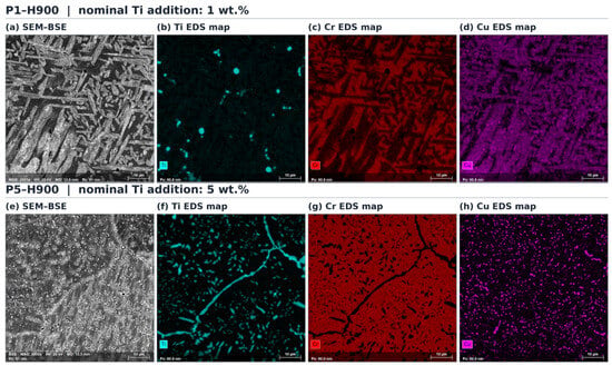
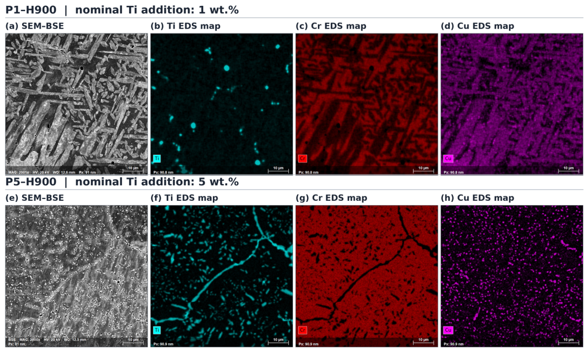
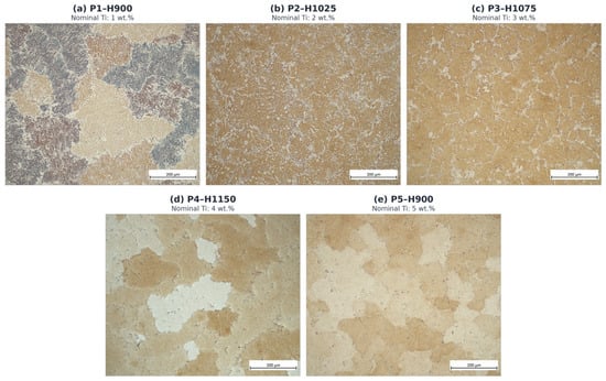
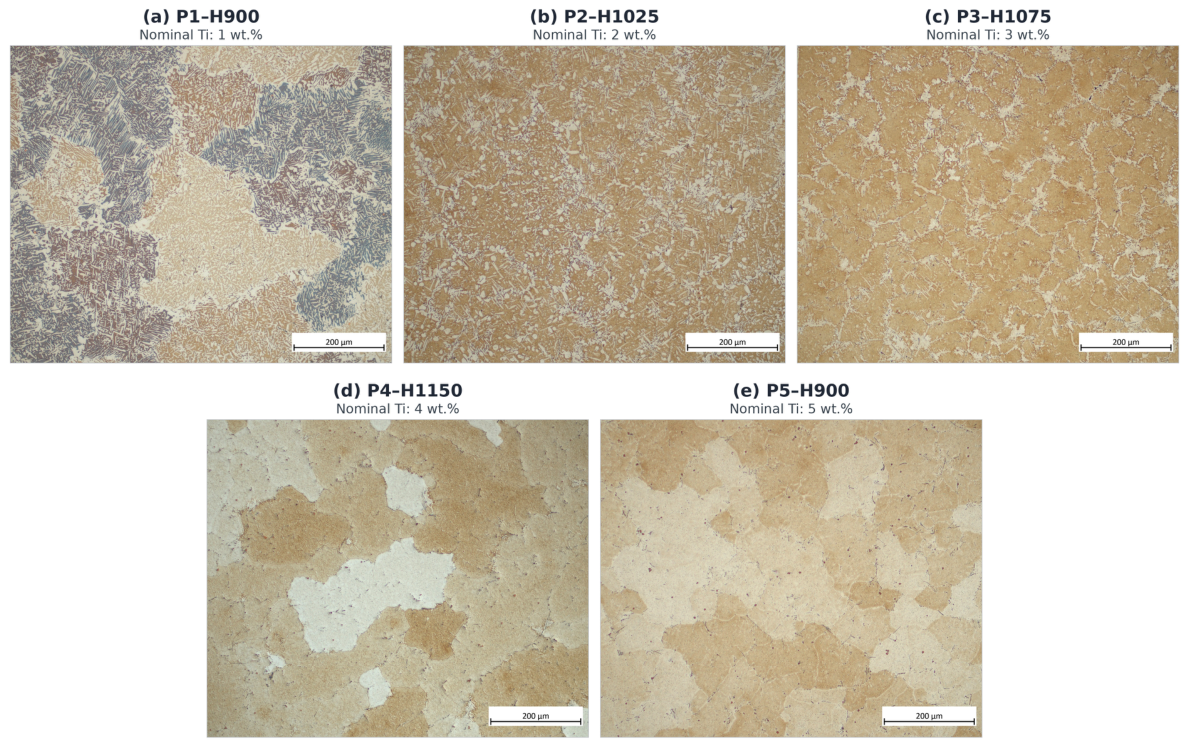
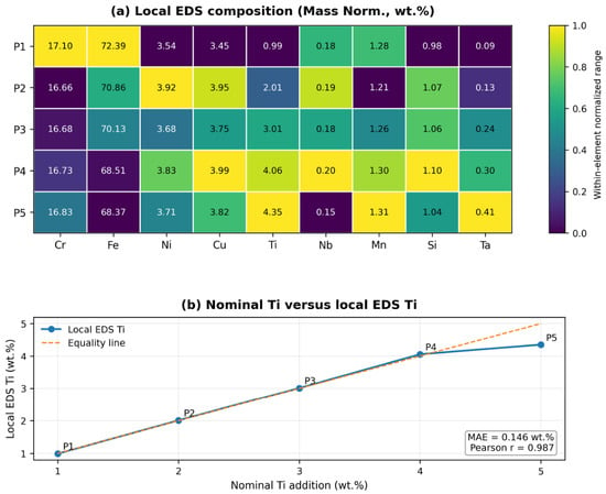
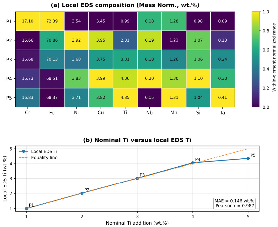
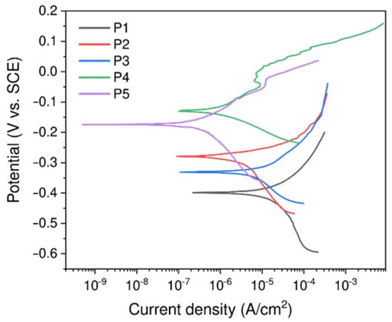
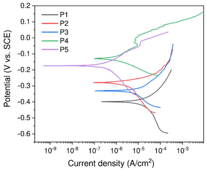
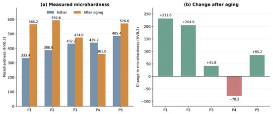
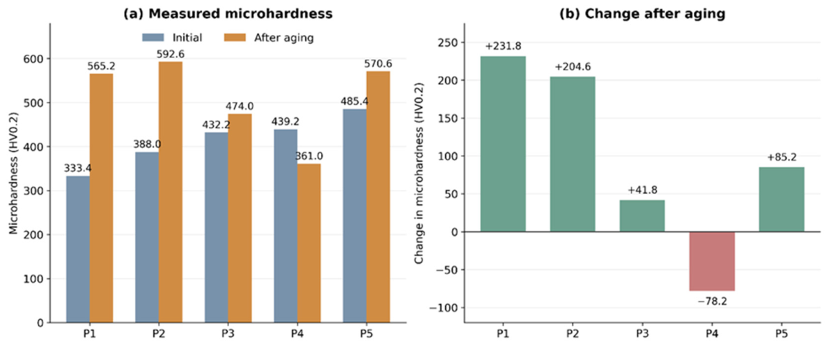
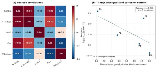
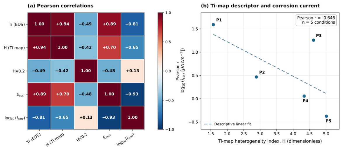
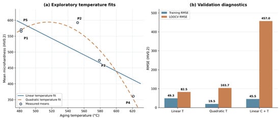
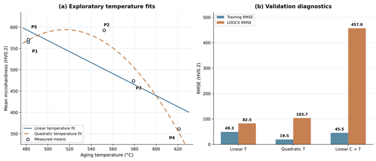
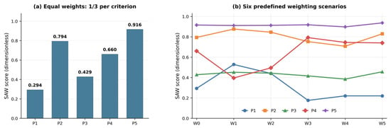
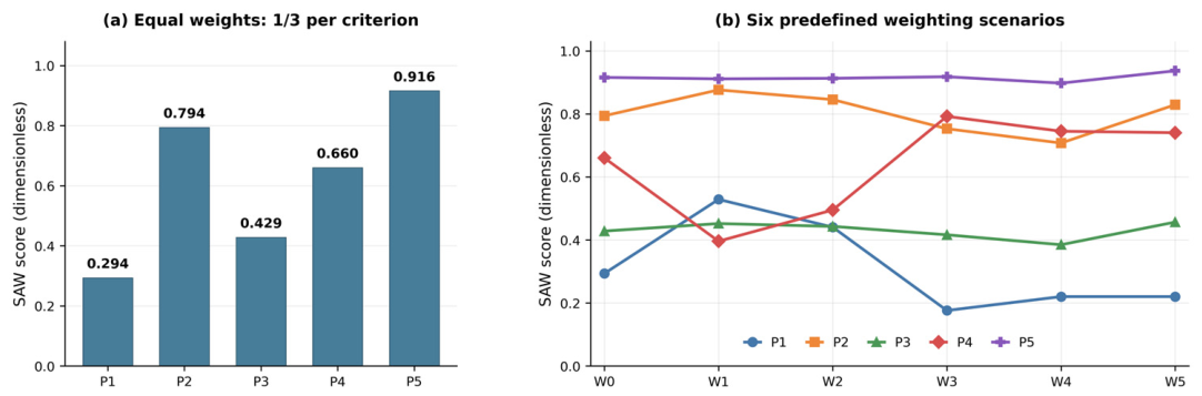

Disclaimer/Publisher’s Note: The statements, opinions and data contained in all publications are solely those of the individual author(s) and contributor(s) and not of MDPI and/or the editor(s). MDPI and/or the editor(s) disclaim responsibility for any injury to people or property resulting from any ideas, methods, instructions or products referred to in the content. |
© 2026 by the authors. Licensee MDPI, Basel, Switzerland. This article is an open access article distributed under the terms and conditions of the Creative Commons Attribution (CC BY) license.