


Simple Summary
Climate change is expected to alter the distribution of grassland insect pests, but comparable evidence for several important species remains limited in Yunnan, southwestern China. We combined extensive provincial census and targeted survey records to examine nine pests using the same modelling and evaluation procedures. Projections covered four consecutive 20-year periods from 2021 to 2100 under three emission pathways and three climate models. Rainfall during the warmest part of the year was the strongest predictor for six species. Suitable areas generally became smaller under the late-century high-emission pathway, although responses differed among species and climate models. The study also identified previously surveyed counties and townships for repeat monitoring. By combining a large local field database with comparable species-level projections, this study provides a basis for tracking distributional changes and coordinating grassland pest surveillance across Yunnan.
Abstract
Climate change may alter grassland pest distributions, yet province-wide comparisons based on extensive field surveys remain limited in Yunnan, China. We analysed 10,342 census and special-survey records, retaining 4281 species–climate-cell records for nine pests. Five WorldClim predictors entered ten-algorithm ensembles weighted by the true skill statistic (TSS), evaluated using nested spatial cross-validation. Three climate models projected SSP1-2.6, SSP2-4.5, and SSP5-8.5 across four 20-year periods spanning 2021–2100. Predictive performance varied among species: area under the receiver operating characteristic curve (AUC) ranged from 0.591 to 0.778, and TSS from 0.198 to 0.365. Pseudoxya diminuta had the highest AUC (0.778), Patanga japonica the highest TSS (0.365), and the 27-cell Holotrichia parallela model the lowest AUC (0.591). Warm-quarter precipitation ranked first for six species, with mean permutation-induced AUC decreases of 0.054–0.145. Baseline threshold-defined suitable area was largest for Oxya chinensis (235.3 × 10³ km2). By 2081–2100 under SSP5-8.5, consensus suitable area declined by 63.4% for P. japonica and 54.6% for P. diminuta. These species-specific climatic associations and projected changes provide a basis for coordinated provincial surveillance, supported by survey-derived county–township revisit priorities.
1. Introduction
Grassland insects respond rapidly to changes in temperature, rainfall, vegetation, and land use. Warming can accelerate development, increase voltinism, or improve overwinter survival, but it can also exceed thermal limits, desynchronise insects from forage, or reduce habitat through altered moisture regimes [1,2,3,4]. Observed range shifts and poleward movement of crop pests show that climate is already reorganising insect distributions, although responses remain taxon- and region-specific [5,6].
Grasshoppers are especially sensitive because embryonic survival depends on soil moisture and temperature, post-embryonic development is strongly thermal, and forage quantity and quality mediate growth and movement. Recent work links distributional change to habitat availability, phenology, elevation, and interannual climate rather than to warming alone [7,8,9,10]. Long-term locust records and grazing experiments further show that precipitation, plant nutrient status, and land management can interact with population processes [11,12]. Accordingly, monitoring systems increasingly combine field surveys, remote sensing, climate anomalies, and predictive mapping [13,14,15].
Species distribution models (SDMs) provide a practical framework for relating occurrences to environmental gradients and projecting potential suitability across space and climate scenarios [16,17,18,19]. Ensemble forecasts combine different response structures and can reduce dependence on one algorithm [20,21,22]. However, algorithm multiplicity does not correct biased sampling or guarantee geographic transfer. Fit-for-purpose SDMs require a stated sampling domain, ecologically defensible background, spatially independent validation, collinearity control, and explicit treatment of extrapolation [23,24,25,26]. Presence-background models are particularly sensitive to pseudo-absence choice, accessibility bias, and clustered records [27,28,29,30].
Grassland pest suitability research increasingly combines climate, vegetation, surface moisture, and topography. Studies document expansion, contraction, and elevational redistribution and support risk zoning in alpine, arid, and temperate grasslands [7,9,31,32,33,34,35]. Four gaps nevertheless limit coordinated surveillance. First, despite existing multi-species studies, province-scale comparisons of multiple grassland pests remain uncommon, particularly those based on extensive, systematically collected field records across Yunnan’s heterogeneous mountains [31,32,35]. Such evidence is needed to establish shared monitoring priorities under one design. Second, many applications rely on a single MaxEnt model and random validation, leaving spatial autocorrelation, between-algorithm differences, and threshold uncertainty incompletely characterised [23,25,27,30]. Third, host resources, biotic interactions, dispersal constraints, and multi-GCM uncertainty are seldom considered together [17,18,19,24,35]. Fourth, regional suitability maps are rarely translated into reproducible county–township monitoring lists that can guide routine surveillance and resource allocation [24,36].
Yunnan Province combines low-latitude monsoon climates with the southeastern Tibetan Plateau and Hengduan Mountains. Its short-distance elevation and moisture gradients support tussock grasslands, shrub-grasslands, dry-hot savannas, montane meadows, and alpine meadows. We examined nine taxa identified as operationally important in the provincial pest census: Acrida cinerea, Gastrimargus marmoratus, Oxya chinensis, Patanga japonica, Phlaeoba infumata, Trilophidia annulata, Atractomorpha sinensis, Holotrichia parallela, and Pseudoxya diminuta [37,38,39]. The focal taxa comprise seven acridid grasshoppers (Orthoptera: Acrididae), A. sinensis (Orthoptera: Pyrgomorphidae), and the scarab H. parallela (Coleoptera: Scarabaeidae: Melolonthinae), providing a comparison across contrasting feeding guilds and grassland associations.
We used a common ensemble framework to address three questions. (1) Where are current suitable areas, and which climatic variables are most strongly associated with their distribution? (2) How do threshold-defined suitable areas and suitability-weighted centroids change across 2021–2040, 2041–2060, 2061–2080, and 2081–2100 under SSP1-2.6, SSP2-4.5, and SSP5-8.5 across MIROC6, BCC-CSM2-MR, and MRI-ESM2-0? (3) How do performance and predictor importance differ among species and algorithms, and which counties and townships warrant repeat monitoring on the basis of existing survey records?
Provincial census and special-survey records provided the primary occurrence data, supplemented by distributional information from GBIF. Using a common modelling framework, we compared habitat suitability, predictive performance, and climatic associations among nine grassland insect pests, and assessed projected changes in suitable area and suitability-weighted centroids. Survey records were also used to identify priorities for repeat monitoring at county and township levels. Together, these analyses can inform species-specific surveillance and the allocation of monitoring resources across Yunnan.
2. Materials and Methods
2.1. Study Area and Climate-Suitability Modelling Framework
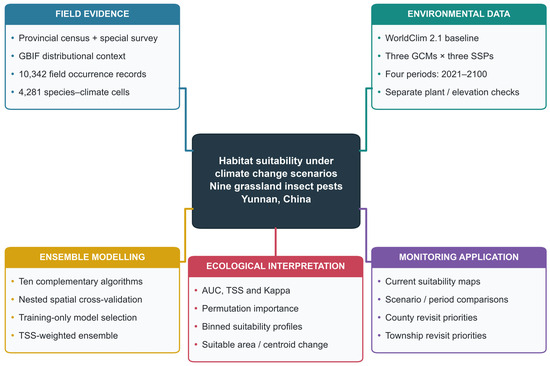
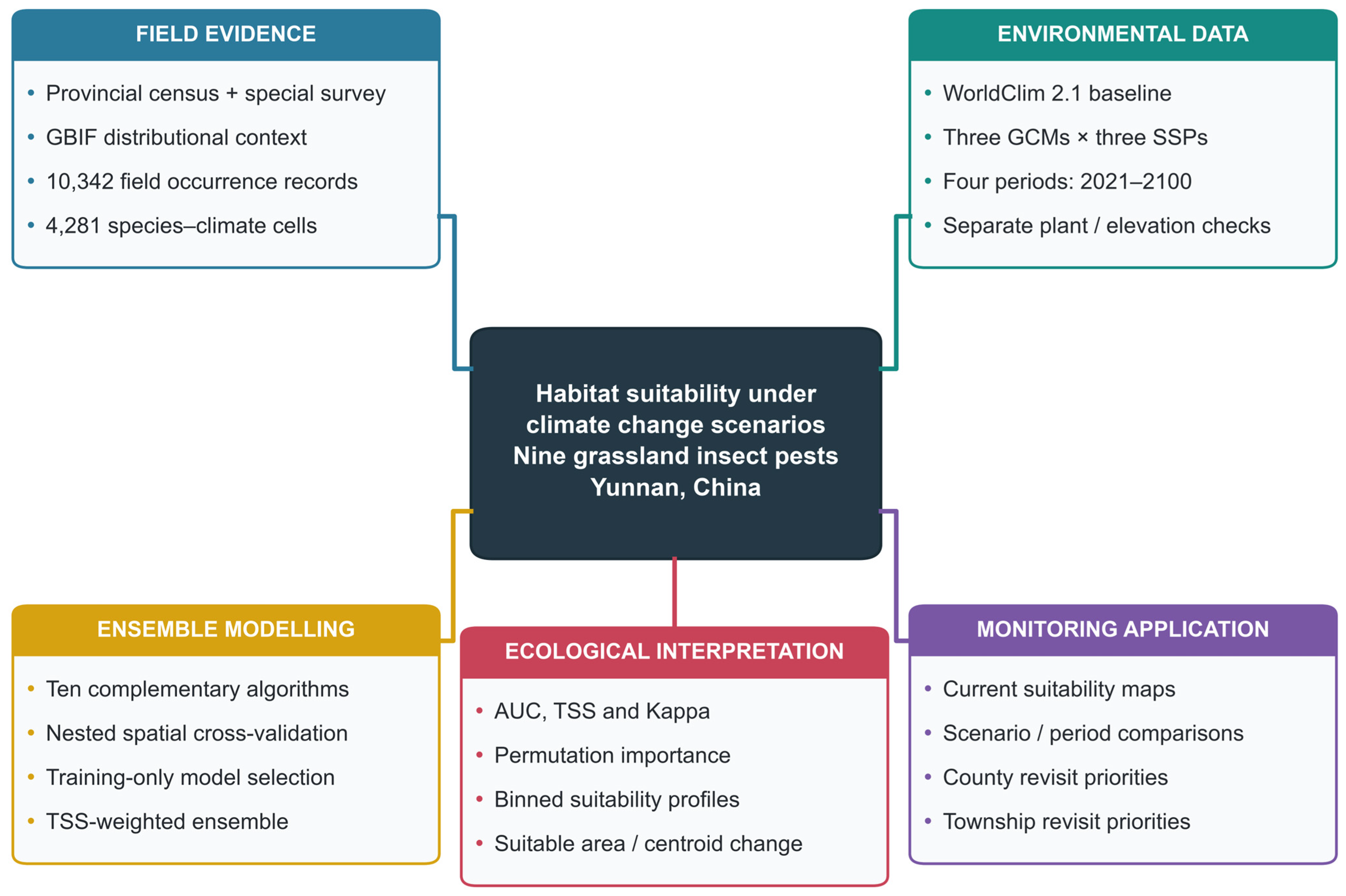
We followed the ODMAP reporting protocol [23]. Predictions from ten algorithms were combined using weights based on inner-validation TSS [20,21,22,40]. Figure 1 outlines the five components of the analysis.
Figure 1.
Analytical workflow for nine grassland insect pests. Five linked modules link field evidence, environmental data, ensemble modelling, ecological interpretation, and monitoring application. Climate projections cover three GCMs, three SSPs, and four periods spanning 2021–2100. Plant and elevation analyses are supplementary; revisit lists are derived separately from survey records. GCM, global climate model; SSP, shared socioeconomic pathway; AUC, area under the receiver operating characteristic curve; TSS, true skill statistic; GBIF, Global Biodiversity Information Facility.
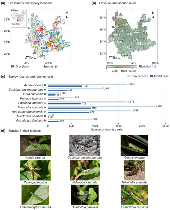
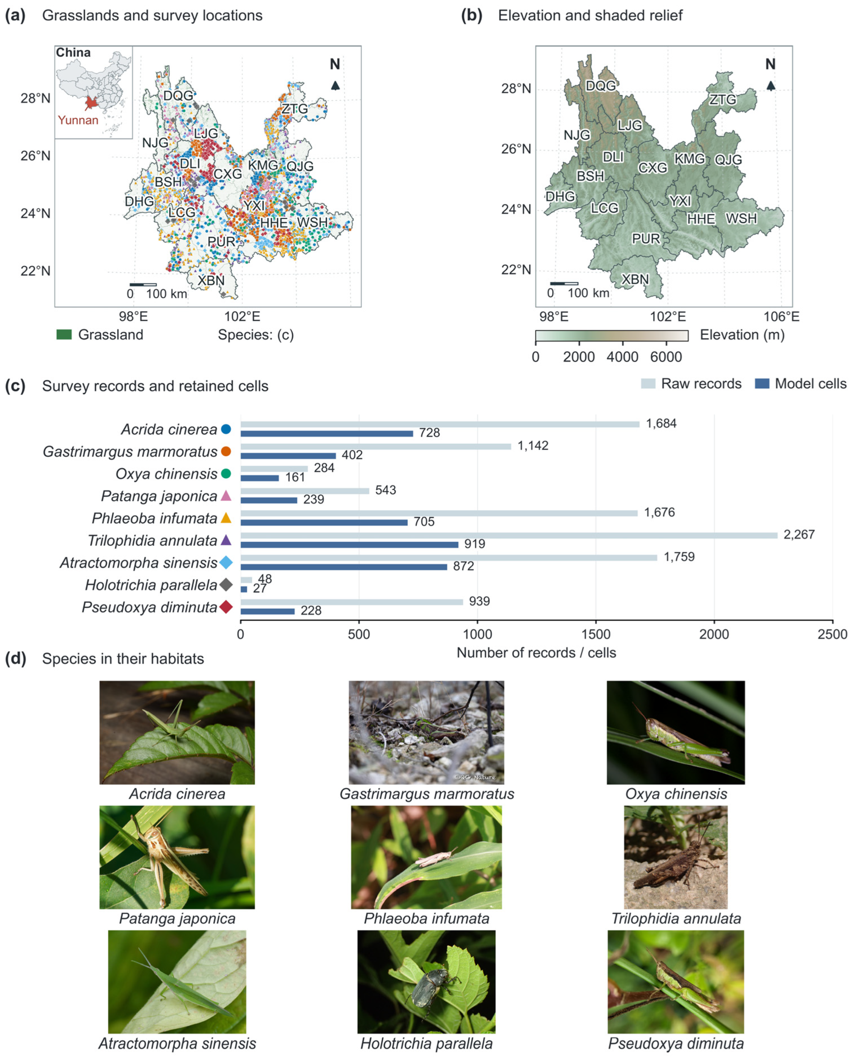
Yunnan is located in southwestern China (approximately 21.1–29.3° N, 97.5–106.3° E) and covers about 394,000 km2. Elevation generally decreases from Northwest to Southeast. Differences in monsoon influence and deeply incised valleys contribute to marked spatial variation in temperature and moisture. Figure 2b shows the terrain using a 30 arc sec digital elevation model (DEM). Across the 19,738 prediction cells at 2.5 arc min resolution, elevation ranges from 162 to 5254 m, with a median of 1819 m.
Figure 2.
Study area, terrain, and target species. (a) Grasslands and retained occurrence cells, with Yunnan located in China in the upper left; species symbols correspond to (c). (b) WorldClim 30 arc sec elevation and shaded relief in CGCS2000 Albers projection. (c) Raw-record and model-cell counts. (d) Ecological photographs of the nine species (sources and licences in the accompanying photograph-credit file). Prefecture codes: KMG, Kunming; QJG, Qujing; YXI, Yuxi; BSH, Baoshan; ZTG, Zhaotong; LJG, Lijiang; PUR, Pu’er; LCG, Lincang; CXG, Chuxiong; HHE, Honghe; WSH, Wenshan; XBN, Xishuangbanna; DLI, Dali; DHG, Dehong; NJG, Nujiang; DQG, Diqing.
2.2. Field Databases and Occurrence Processing
2.2.1. Provincial Grassland Pest Census
The provincial census began in December 2020, with fieldwork during 2021–2024 across 16 prefectures and 129 grassland-containing counties. Reconnaissance routes and standard plots represented alpine and montane meadows, warm and tropical tussock grasslands, dry-hot savannas, and sown grasslands. Methods included quadrats, soil pits, sweep-net transects, standardised plant units, and supplementary traps. Records documented coordinates, pests, vegetation, abundance or damage, photographs, and specimens. County, prefectural, and provincial quality checks and expert identification preceded release [37]. The programme comprised 2210 routes, 98,956 route points, 13,264 plots, and 76,959 quadrats or transects. The extraction used 30,641 valid standard-plot pest rows and 24,690 reconnaissance rows.
2.2.2. Provincial Grasshopper Special Survey
The 2025 grasshopper special survey sampled natural and sown grasslands and agro-pastoral ecotones, emphasising historical occurrence areas, frequent census localities, and representative habitats. Route reconnaissance, plots, sweep-net transects, visual counts, and quadrats documented life stage, density or damage, vegetation, coordinates, elevation, photographs, and specimens. Difficult taxa underwent morphological examination, selected DNA comparison, and expert identification following national survey specifications [38,41,42]. The collection and identified-specimen tables contained 637 and 369 records, respectively; 71 identified records matched the target taxa.
2.2.3. Harmonisation, Filtering, and GBIF Context
Species names and prefecture, county, and township fields were standardised across the two survey programmes. After excluding records with invalid coordinates or locations outside Yunnan, 10,342 target-pest records remained: 6518 from standard plots, 3753 from reconnaissance, and 71 from the special survey. Excluding 73 records assigned to boundary cells outside the prediction mask and retaining one occurrence per species per 2.5 arc min cell yielded 4281 species–cell records (27–919 per species; Table 1). For duplicate species–cell records, identified special-survey specimens took precedence over standard-plot and reconnaissance records, in that order. Target species were selected based on provincial survey findings, geographic coverage, grassland associations, and contrasting feeding guilds, rather than an abundance ranking.
Table 1.
Target-pest records and frequently recorded associated plants in the provincial survey archive.
The GBIF Occurrence Search portal (https://www.gbif.org/occurrence/search) (accessed on 4 July 2026) supplied public-distribution context [43]. Searches within the approximate Yunnan boundary returned 65 records for the 9 pests and 1483 records for 13 associated plant categories. Differences in coverage, sampling, and record independence precluded pooling these records with local occurrences or treating them as independent validation.
2.3. Background Sampling and Associated Plant Information
2.3.1. Pseudo-Absence/Background Sampling
Background cells were sampled uniformly without replacement within the provincial mask, excluding focal-species occurrence cells [27,28]. Sample size was max(120, 3n), where n is the occurrence-cell count: a 3:1 ratio for eight taxa and 120:27 for H. parallela. Supervised classifiers used inverse-frequency weights to equalise class totals; SREs and EDM used presences only. Background represents available environments, not confirmed absence. Sensitivities tested alternative quantities, survey-weighted sampling, and exclusion of the training-presence 2.5th–97.5th percentile envelope. A nested RF comparison held samples and tuning grids constant to assess class weighting (Table S10).
2.3.2. Associated Plant Sensitivity Models
Field plant records mix feeding observations, associated species, and dominant vegetation. Supplementary plant indices therefore used only outer-training data: five frequent plant categories were selected within each training fold, then their detections were smoothed at 17.5, 35, and 70 km and divided by similarly smoothed survey-site density. Outer-test sites were excluded. These effort-normalised indices describe associated-plant context, not measured cover, biomass, or confirmed host specificity [44,45,46]; they were not primary predictors.
A separate RF predicted the occurrence of selected plant categories from training-fold climate data. This score entered a supplementary pest RF, with future scores either held static or recalculated under future climate.
2.4. Environmental Predictors and Climate Scenarios
WorldClim 2.1 baseline normals (1970–2000) and CMIP6 projections were aligned at 2.5 arc min [47,48]. Cell areas were calculated by latitude. MIROC6, BCC-CSM2-MR, and MRI-ESM2-0 supplied SSP1-2.6, SSP2-4.5, and SSP5-8.5 for four consecutive periods: 2021–2040, 2041–2060, 2061–2080, and 2081–2100 (36 combinations). Each projection used unchanged fitted models, weights, and thresholds; no temporal interpolation was applied. Late-century maps summarise the endpoint; all periods are reported in Figures S3 and S4 and Table S12. Monthly 10 arc min data from the same three GCMs describe baseline and late-century seasonal context (Figure 10). Monthly temperature was (minimum + maximum)/2. Precipitation minus Hargreaves reference evapotranspiration (P − ET0) summarised the climatic water balance for May–October and November–April [49] (Table S11).
Candidates represented developmental and seasonal thermal constraints (bio1, bio2, bio4), moisture and vegetation-related conditions (bio12, bio15, bio18), and elevation [7,8,9,10,11,12,31,32,33,34,50,51,52,53,54] (Table 2). On the provincial grid, bio12 correlated strongly with bio18 (Spearman ρ = 0.95), and elevation with bio1 (ρ = −0.90); candidate VIFs reached 88.23. We retained bio1, bio2, bio4, bio15, and bio18 (maximum |ρ| = 0.68; VIF 1.72–3.17), favouring warm-season moisture and explicit thermal conditions over redundant annual precipitation and static elevation [29]. Screening used environmental data, not test-fold performance. Coordinates were excluded. Elevation was assessed separately in RF sensitivity models at 2.5 arc min (Table S9); the finer Figure 2b DEM serves cartographic purposes only.
Table 2.
Environmental predictors and supplementary covariates.
2.5. Algorithms and TSS-Weighted Ensemble
Ten algorithms represented complementary assumptions: linear and quadratic logistic models (GLM, QGLM), Gaussian naive Bayes (GNB), surface range envelopes (SREs), environmental distance (EDM), feature-logistic classification (FLC), random forests (RFs), gradient boosting (GBM), classification trees (CTA), and artificial neural networks (ANNs). Table 3 reports implementations and search grids. FLC used standardised linear, squared, and positive-hinge features at −1, 0, and 1 SD with L2-regularised logistic regression; it is distinct from MaxEnt [55,56,57]. RF and GBM represented bagged and sequentially boosted tree ensembles, respectively [40,58,59,60]. Scaling was fitted separately within every training partition.
Table 3.
Algorithms and principal settings used in the ensemble.
The bounded grid contained 36 configurations per outer fold (1620 candidate evaluations, each with three inner fits); RF tree count (200) and boosting stages (150) were fixed. ANN used five standardised inputs, one hidden layer with 12 or 24 rectified-linear units, and a logistic output. L-BFGS minimised class-weighted binary cross-entropy with an L2 penalty (alpha = 0.1 or 1); these four configurations were selected by inner-validation TSS [40]. Training allowed 5000 iterations and 100,000 function evaluations at tolerance 10−4.
All 540 inner and 45 selected outer fits completed without convergence warnings. Two additional initialisations per selected outer fit held architecture, penalties, samples, and thresholds fixed (90 fits; Table S13). No test-based seed selection was performed. A separate nine-algorithm ensemble excluded ANN, renormalised the remaining inner-TSS weights, and selected its own inner threshold (Table S10).
Nested spatial cross-validation separated selection from evaluation [25,26,61]. Approximately 75 km blocks were allocated to five outer folds and three inner folds within each outer-training set. The setting maximising pooled inner TSS was refitted to outer-training data. Non-negative inner TSS values were normalised as algorithm weights, and the ensemble threshold maximised inner TSS. Outer-test data were excluded from scaling, tuning, threshold selection, and weighting. AUC, TSS, and Kappa were calculated on each held-out outer fold using its fixed threshold [62,63,64,65]. Maps average five outer-training ensembles.
2.6. Model Evaluation and Ecological Interpretation
Performance is reported as mean ± sample SD across five outer folds (Table 4; Table S1). Importance is the decrease in outer-test ensemble AUC over five permutations per predictor per fold; negative values were retained without normalisation. Figure 3 shows Tukey boxplots of occurrence-cell environmental values. Marginal profiles average baseline predictions within 18 equal-width bins spanning the provincial 2nd–98th predictor percentiles.
Table 4.
Outer-fold performance of the nested TSS-weighted ensemble.
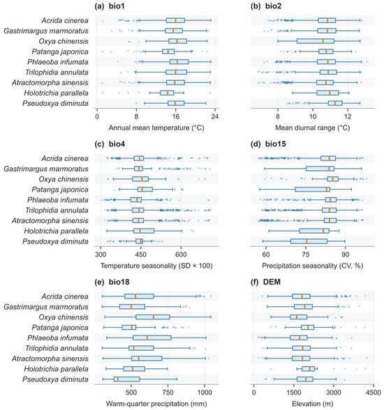
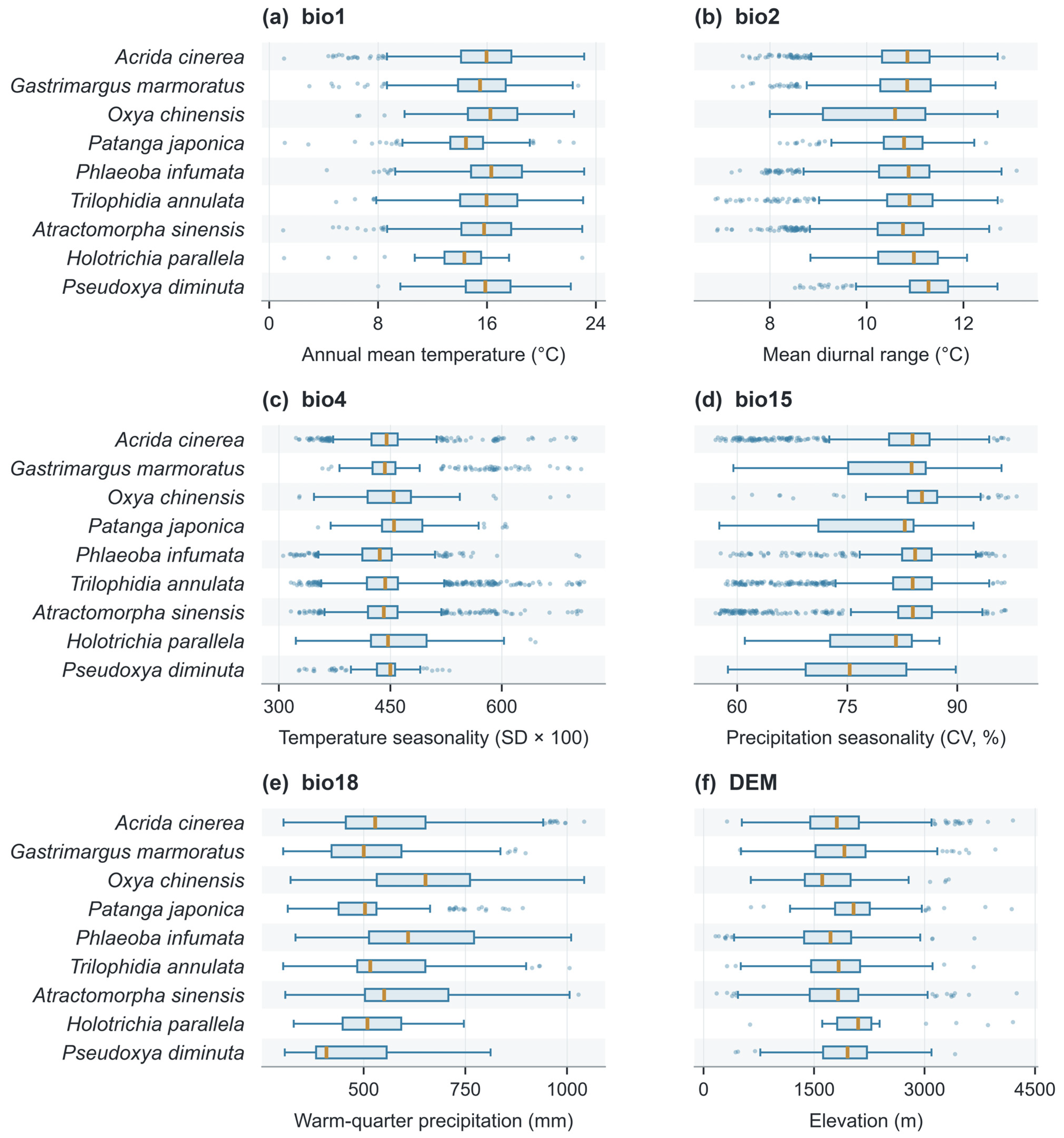
Figure 3.
Occurrence-cell distributions of (a) bio1, (b) bio2, (c) bio4, (d) bio15, (e) bio18, and (f) elevation. Boxes span the first to third quartiles; amber lines mark medians. Whiskers extend to the most extreme observations within 1.5 interquartile ranges, and dots show outliers. Species sample sizes, from top to bottom, are 728, 402, 161, 239, 705, 919, 872, 27, and 228.
Controlled RF sensitivities used 100 trees, maximum depth 6, minimum leaf size 5, balanced weights, and a fixed 0.5 threshold. Comparisons varied elevation, bio12, background quantity and selection, plant-index bandwidth, or climate-conditioned plant context while retaining the same outer-test samples. They are diagnostic comparisons, separate from the nested ensemble evaluation.
2.7. Climate Projections, Centroids, and Administrative Priorities
The mean inner-validation TSS threshold t defined suitable areas in consensus maps. The four display classes (unsuitable, low, moderate, and high) were bounded by t/2, t, and (1 + t)/2; moderate and high jointly define threshold-positive area. Sensitivity analyses used the mean inner-validation 10th-percentile presence threshold and a fixed score of 0.5. These classes represent relative model scores, not observed infestation.
Centroids were weighted by suitability × cell area within threshold-positive cells; displacement used WGS84 geodesics. For every species, period, and pathway, 1000 resamples of five fitted folds and three GCMs provided conditional 95% percentile intervals. Baseline and future used matched resampled fold weights. Undefined centroids were excluded and counted. These intervals describe model–GCM variation, not insect migration. Weighted directional agreement among algorithm–fold–GCM members is mapped separately for late-century SSP5-8.5 (Figure S5). Agreement values for all three pathways accompany the spatial data; values below 80% indicate lower agreement.
County and township revisit indices were calculated separately from a 5210-record, approximately 1 km grid-filtered survey archive: I = 20S + 12 ln(N + 1), where S is recorded target-species richness and N is record count. H. parallela was excluded from both quantities because evidence was sparse. The richness coefficient was varied from 10 to 40; rank correlations and top-ten overlap assessed stability. Survey effort affects these descriptive revisit priorities. All twenty displayed units were matched to administrative polygons by name and code.
2.8. Reproducibility
Data preparation, modelling, evaluation, and figure production were implemented in Python 3.12 with NumPy 2.5.3 and scikit-learn 1.9.1 [40], using master seed 20260912. Accompanying machine-readable outputs retain climate-cell occurrences, fold assignments, model metrics, variable importance, marginal profiles, suitability areas, centroid shifts, and county–township revisit rankings. Code documents seed offsets, settings, and resampling procedures.
3. Results
3.1. Occurrence Evidence for Suitability Modelling
After filtering and deduplication at 2.5 arc min resolution, 4281 species–cell records remained from 10,342 survey records, covering 2698 geographic cells and 119 counties across all 16 prefectures (Table 1; Figure 2a,c). Sample sizes ranged from 27 cells for H. parallela to 919 for T. annulata. Four species, T. annulata, A. sinensis, A. cinerea, and P. infumata, accounted for 75.3% of the modelling records.
Environmental conditions differed among species (Figure 3; Table S9). Median warm-quarter precipitation was 652 mm for O. chinensis and 609 mm for P. infumata, compared with 408.5 mm for P. diminuta. Median annual mean temperature ranged from 14.3 °C for H. parallela to 16.3 °C for P. infumata, while median climate-grid elevation ranged from 1609 m for O. chinensis to 2098 m for H. parallela.
3.2. Model Accuracy and Algorithm Comparison
Mean ensemble AUC ranged from 0.591 ± 0.142 for H. parallela to 0.778 ± 0.124 for P. diminuta; P. japonica reached 0.751 ± 0.028 (Table 4). TSS ranged from 0.198 to 0.365, with the maximum for P. japonica. For H. parallela, TSS was 0.270 ± 0.168 and Kappa 0.105 ± 0.058. Sparse test presences and substantial fold variability limit its map to exploratory interpretation.
ANN had the highest mean single-algorithm AUC (0.729; TSS 0.304), compared with 0.700 for the ensemble and 0.697 for RF (Table 4 and Table S1). Mean ANN weights were 7.1–18.3%. Original and additional initialisations yielded mean AUCs of 0.729, 0.727, and 0.727; G. marmoratus showed the widest species-level range (0.720–0.762; Table S13). Retaining ANN increased ensemble AUC by 0.0165 and TSS by 0.0301 relative to the matched nine-algorithm ensemble (Table S10).
3.3. Species-Specific Predictor Importance
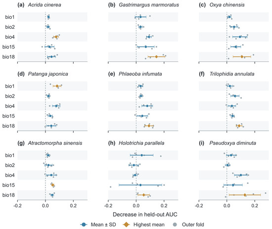
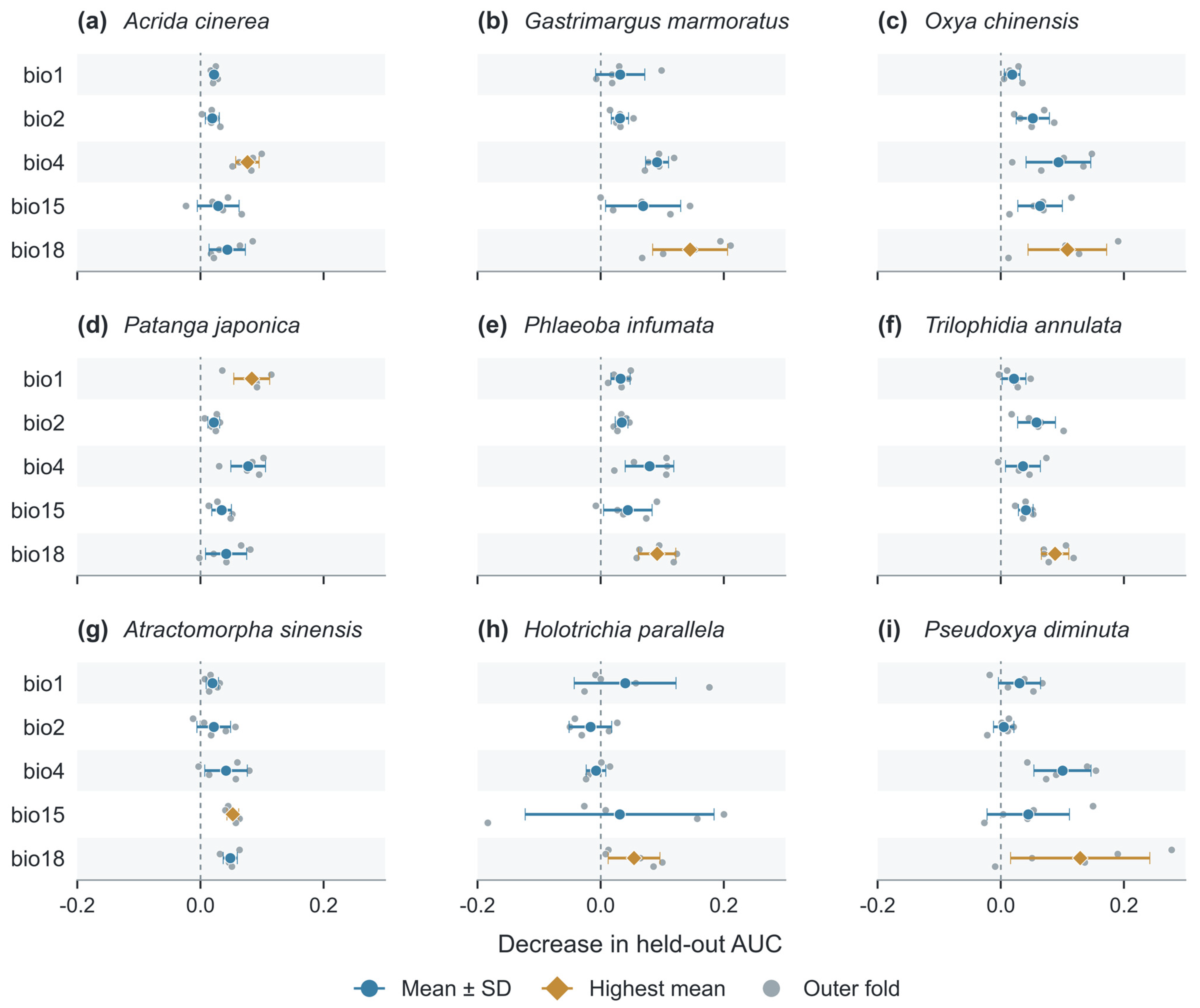
Warm-quarter precipitation (bio18) produced the largest average held-out AUC decrease for G. marmoratus (0.145), O. chinensis (0.108), P. infumata (0.092), T. annulata (0.088), H. parallela (0.054), and P. diminuta (0.129). Other leading predictors were bio4 for A. cinerea (0.076), bio1 for P. japonica (0.083), and bio15 for A. sinensis (0.053). Figure 4 reports the fold-level values, means, and SDs for every species and predictor; several intervals include zero.
Figure 4.
Species-specific held-out permutation importance. Panels (a–i) follow Table 1. Large symbols and horizontal lines show means ± sample SD across five outer folds; small grey points show the individual fold means, each based on five permutations. Amber diamonds identify the highest mean importance within each species; blue circles show the remaining predictors. All panels share one scale. Negative decreases are retained without normalisation. Predictor definitions are in Table 2.
Importance measures predictive association rather than causation. Variables were screened by ecology and collinearity, not test-fold importance. Adding elevation in controlled RF models changed mean AUC from 0.699 to 0.705 (unrounded increment 0.0067), but the mean gain across the eight grasshoppers was only 0.0004. H. parallela increased from 0.511 to 0.568, remaining weakly discriminated; O. chinensis declined from 0.740 to 0.729. Adding bio12 yielded a mean AUC of 0.704 (Table S3); elevation comparisons are detailed in Table S9.
3.4. Baseline Suitability Patterns
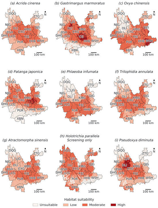
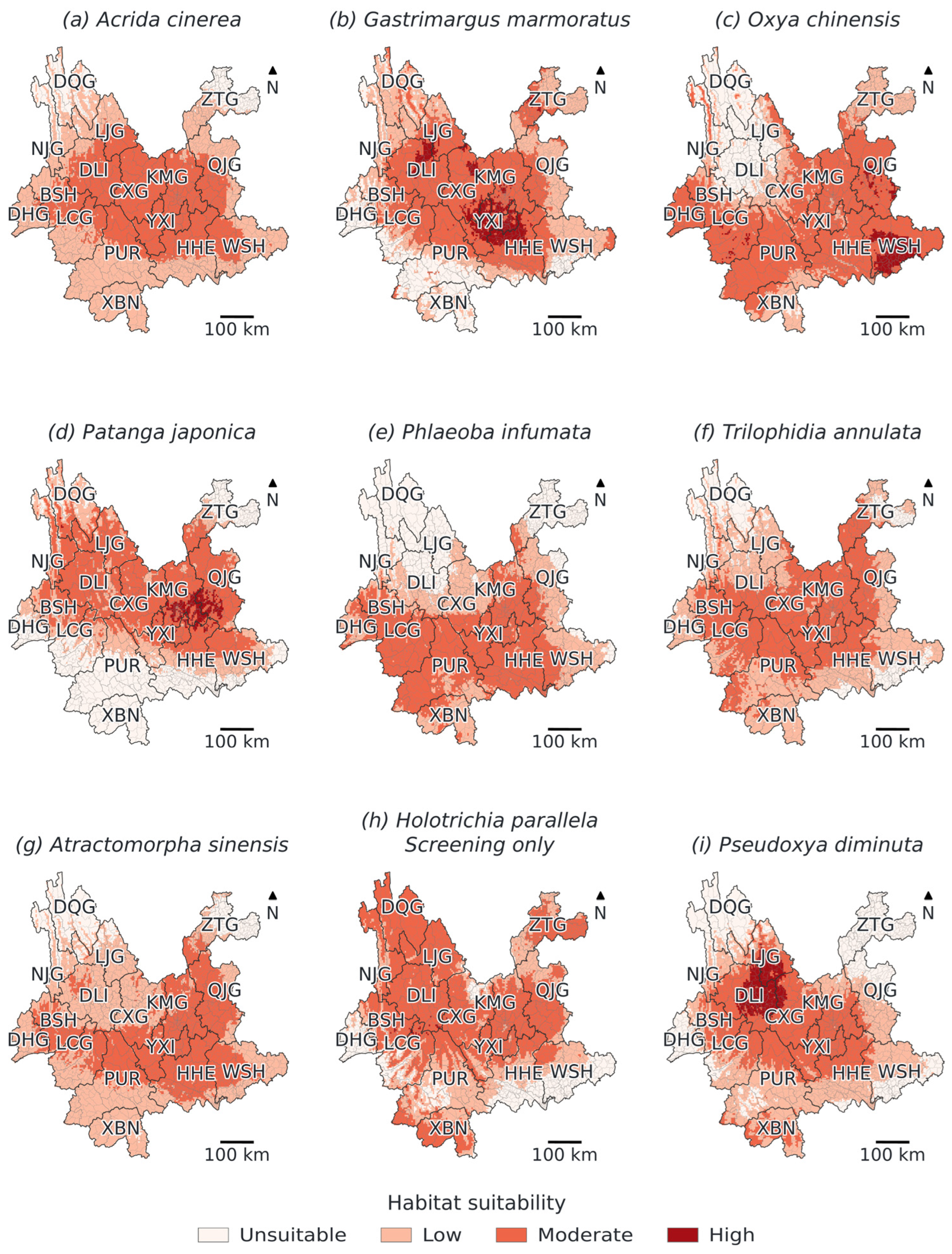
Under baseline climate, consensus threshold-positive area among the eight grasshoppers ranged from 153.3 × 10³ km2 for A. sinensis to 235.3 × 10³ km2 for O. chinensis (Table 5; Figure 5). The H. parallela estimate was 222.8 × 10³ km2; weak discrimination prevents interpreting it as a reliable occupied range.
Table 5.
Consensus threshold-positive area, late-century area change, and SSP5-8.5 centroid displacement.
Figure 5.
Baseline suitability under 1970–2000 normals. Panels (a–i) follow Table 1. The four classes (unsuitable, low, moderate, and high) are separated by t/2, t, and (1 + t)/2, where t is the mean inner-validation TSS threshold; moderate and high define suitable area. Fine and heavy lines mark townships and prefectures. H. parallela is exploratory. Prefecture codes follow Figure 2.
Threshold-positive areas were not restricted to a single shared provincial core. They extended across central plateaus and basins, southern and southeastern sectors, and species-dependent western and northern areas. The totals describe the provincial analysis mask, not grassland actually occupied by each pest. Locally unsuitable land cover and the absence of a dynamic grassland mask constrain their interpretation.
3.5. Future Suitability Under Climate Change Scenarios
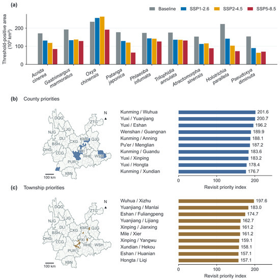
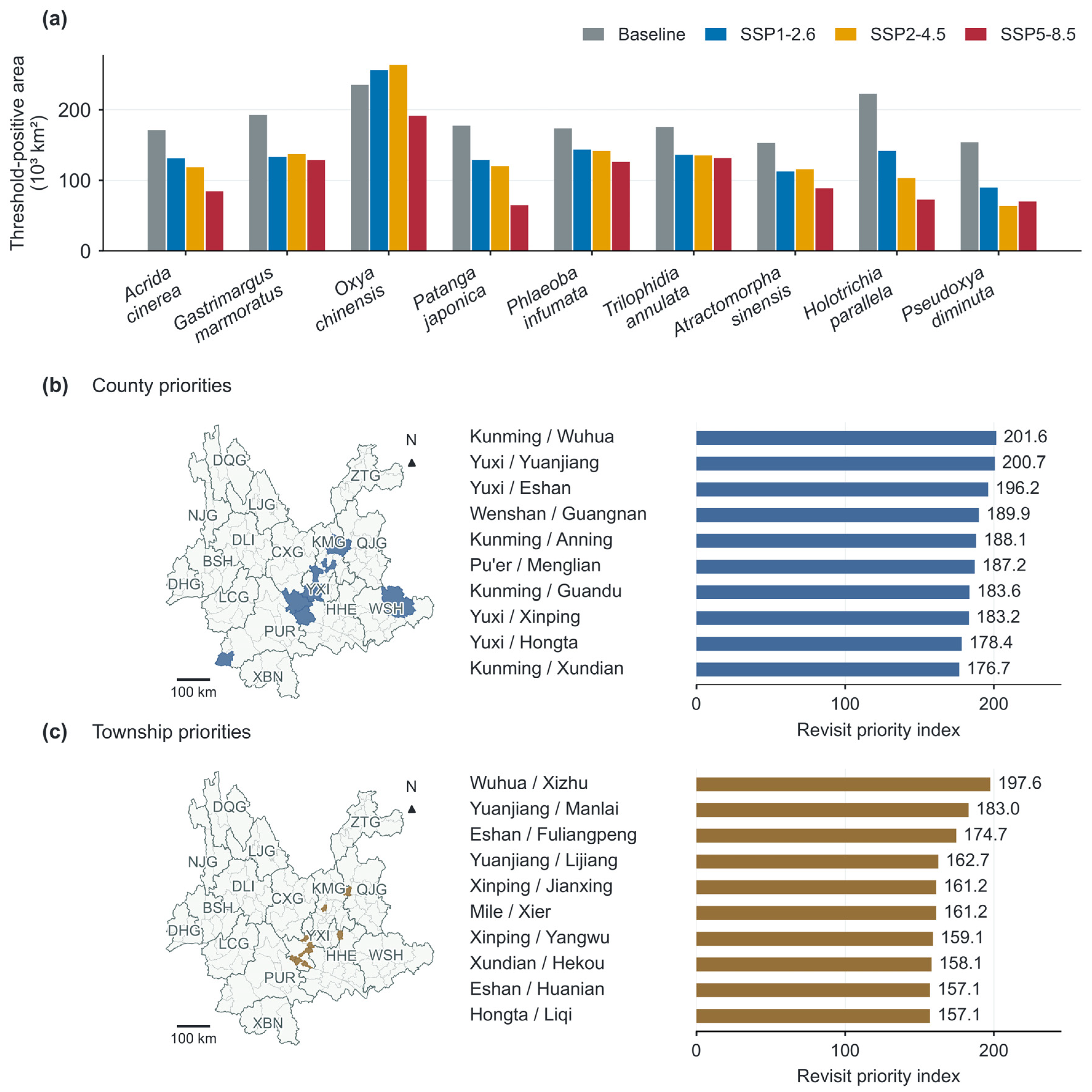
Across the four periods, responses were species-specific rather than uniformly progressive (Figure S3; Table S12). Under SSP5-8.5, P. japonica area changes were −16.2% in 2021–2040, −39.0% in 2061–2080, and −63.4% in 2081–2100; corresponding P. diminuta changes were −51.8%, −50.4%, and −54.6%. Late-century comparisons use the same period across pathways (Table 5; Figure 6 and Figure 7a).
Figure 6.
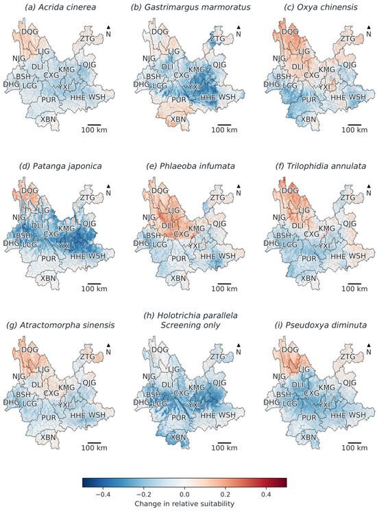
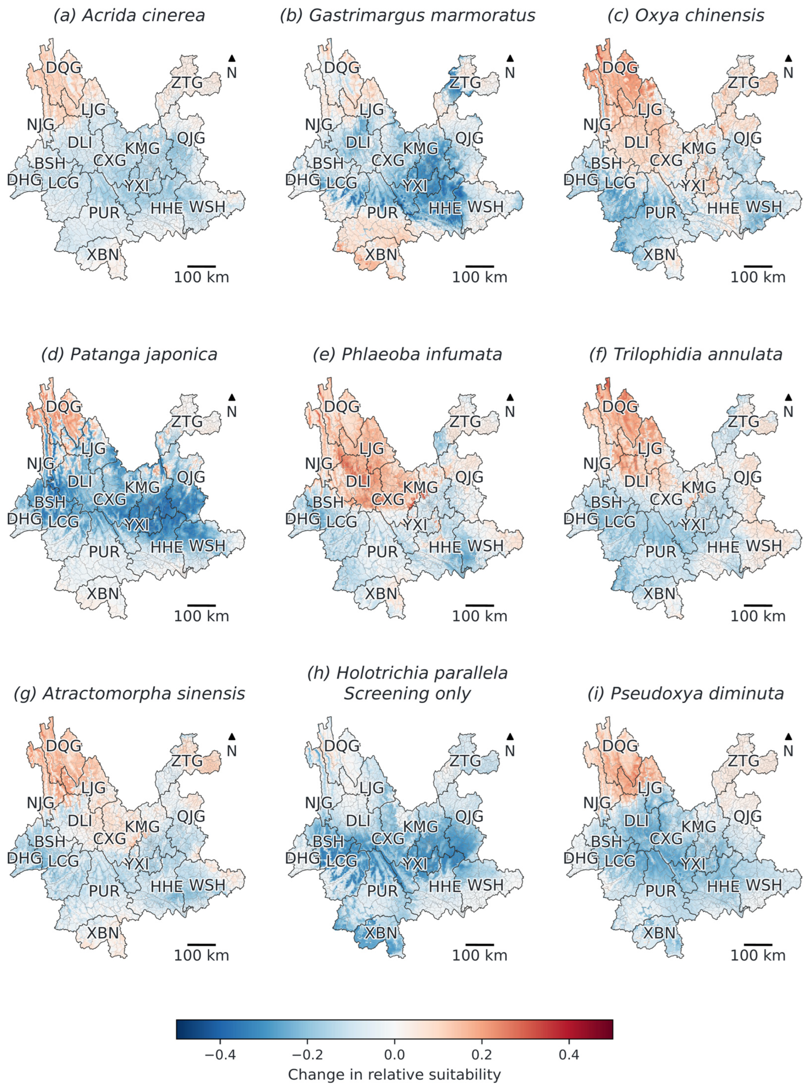
Consensus change in relative suitability under SSP5-8.5 for 2081–2100, compared with baseline climate. Panels (a–i) follow Table 1. Positive values indicate an increase in model score. Weighted directional agreement is shown separately in Figure S5. Township boundaries are shown as fine lines. The H. parallela panel is exploratory only; Figures S1 and S2 provide the other emission pathways.
Figure 7.
(a) Baseline and late-century consensus suitable areas. (b,c) Filled polygons and revisit indices for the ten highest-ranked counties and townships. Lists use prefecture/county and county/township names, respectively. Maps use CGCS2000 Albers projection; prefecture codes follow Figure 2.
Under SSP5-8.5, all nine consensus maps had smaller threshold-positive areas than baseline: A. cinerea -50.7%, G. marmoratus −33.2%, O. chinensis −18.5%, P. japonica −63.4%, P. infumata −27.4%, T. annulata −25.0%, A. sinensis −42.2%, H. parallela −67.3%, and P. diminuta −54.6%. Individual fold–GCM estimates nevertheless differed greatly; for G. marmoratus, future area ranged from 1.9 to 277.3 × 10³ km2. Consensus contraction therefore does not imply unanimous member agreement.
Change maps include local increases and decreases (Figure 6, Figures S1 and S2); SSP5-8.5 directional agreement is mapped separately in Figure S5. BCC-CSM2-MR projected substantially more precipitation: late-century SSP2-4.5 median annual rainfall was approximately 1545 mm versus 1024.5 mm at baseline. An independent monthly source total (approximately 1549 mm) corroborated this climate-model difference.
3.6. Marginal Associations, Centroid Shifts, and Revisit Priorities
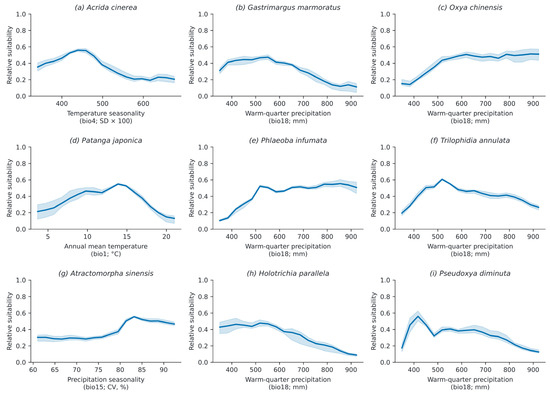
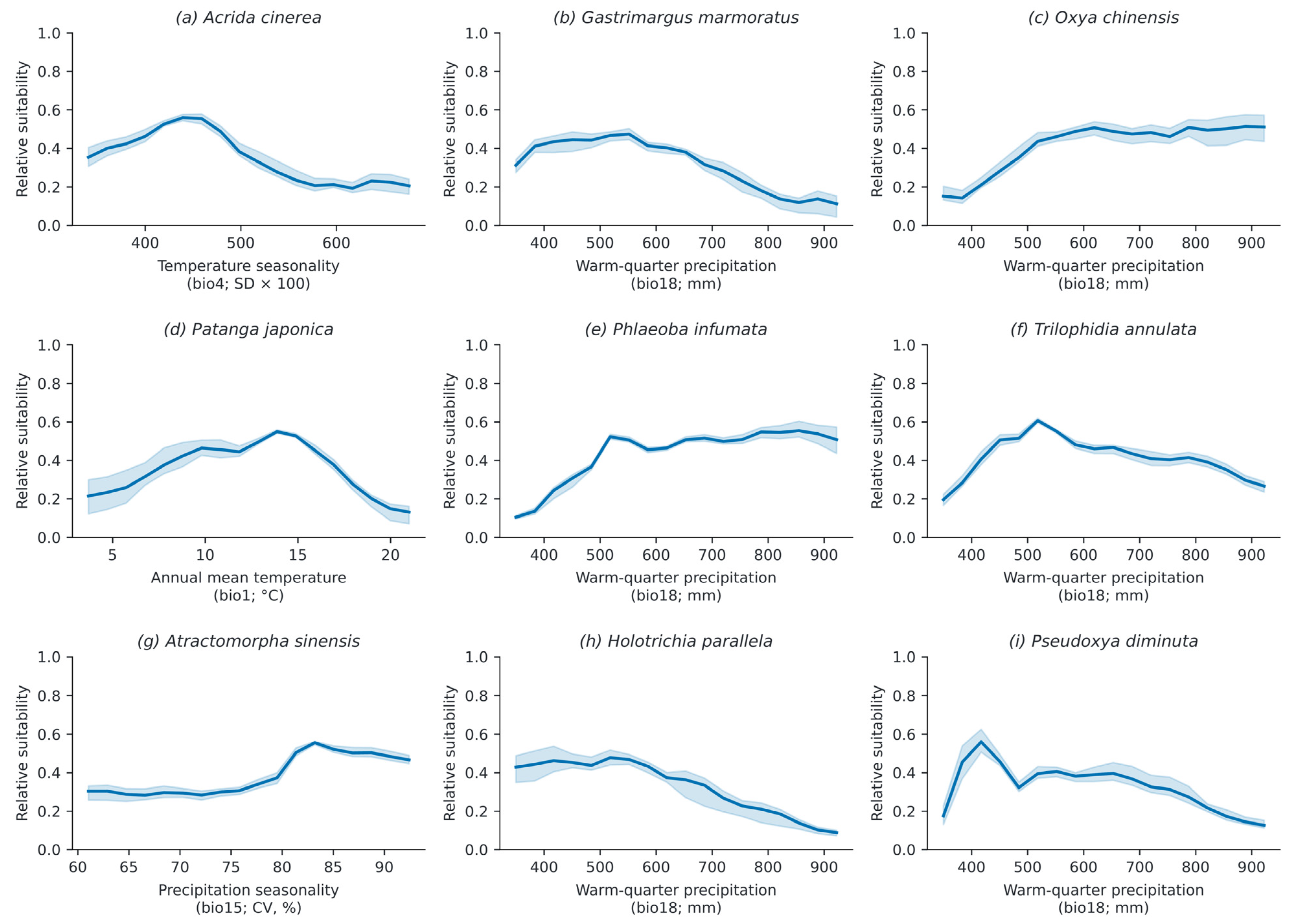
Binned predictor–suitability profiles differed among species (Figure 8). Each displays the highest-importance predictor. Because other environmental conditions co-vary across the grid, turning points cannot be interpreted as physiological optima or isolated predictor effects.
Figure 8.
Binned marginal associations for each species’ highest-importance predictor. Panels follow Table 1. Lines show five-fold means; shading spans fold minima–maxima. Eighteen bins cover the provincial 2nd–98th predictor percentiles. Bin counts are archived.
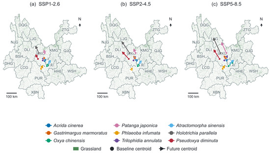
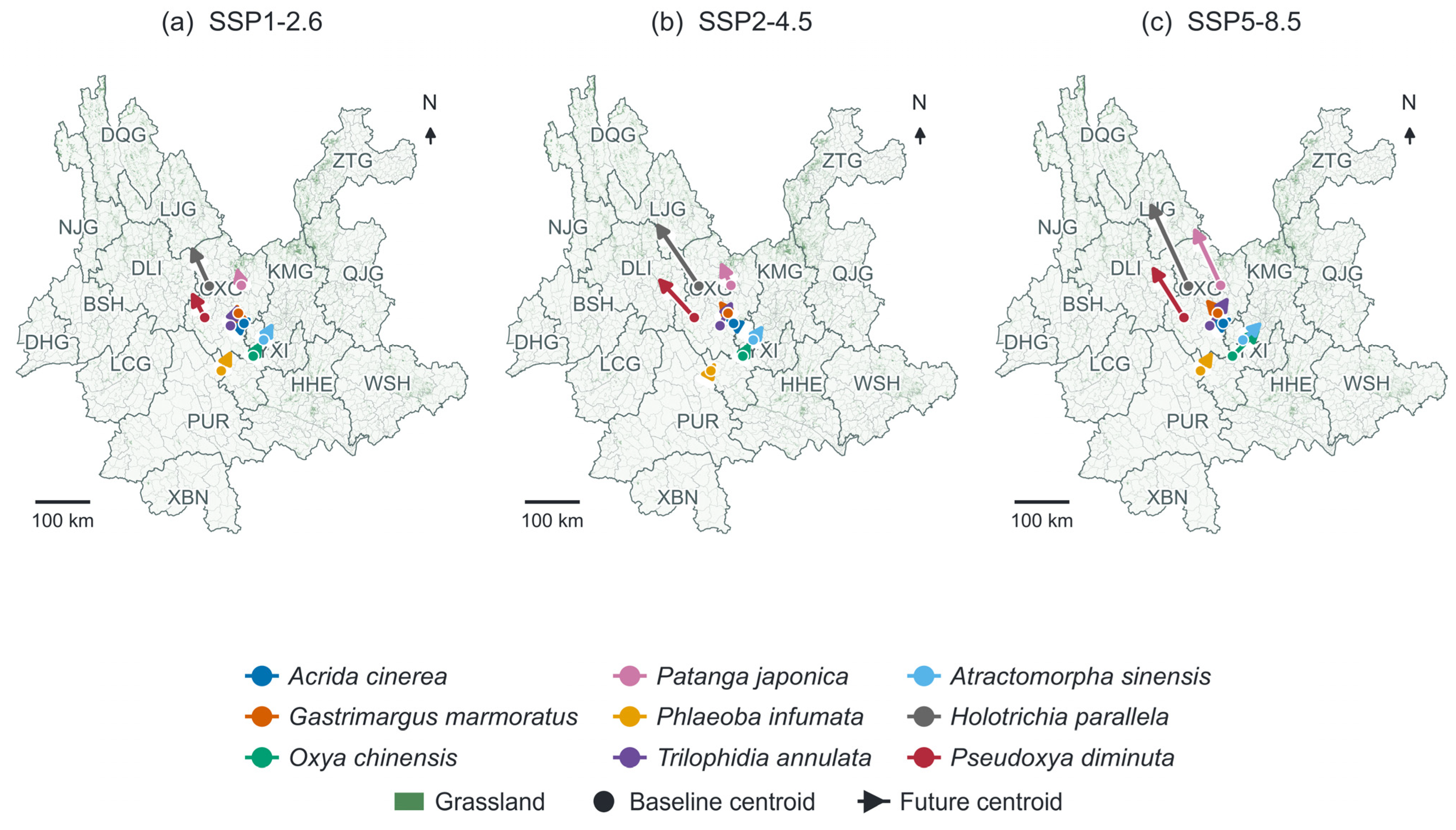
Late-century SSP5-8.5 centroid displacement ranged from 31.6 km (A. cinerea) to 139.0 km (P. japonica) among grasshoppers. Conditional intervals were 90.1–299.8 km for P. japonica and 25.8–407.2 km for G. marmoratus (consensus 49.7 km). One A. cinerea and 32 P. diminuta resamples lacked threshold-positive cells and were excluded from intervals (Table S6; Figure 9). All-period centroid estimates are in Figure S4 and Table S12.
Figure 9.
Late-century suitability-weighted centroids under (a) SSP1-2.6, (b) SSP2-4.5, and (c) SSP5-8.5. Circles mark baseline centroids and arrows point to future centroids; colours distinguish species. Green shows grassland context, with township and prefectural boundaries. Maps use CGCS2000 Albers, geodesic scales, and true north. Conditional intervals are in Table S6; all periods appear in Figure S4. H. parallela remains exploratory.
County indices were highest in Wuhua, Kunming (201.6), Yuanjiang, Yuxi (200.7), and Eshan, Yuxi (196.2); township indices were highest in Xizhu (197.6), Manlai (183.0), and Fuliangpeng (174.7). Varying the richness coefficient from 10 to 40 retained both top-ten lists; minimum rank correlations were 0.9846 for counties and 0.9956 for townships. Survey-effort bias remains (Figure 7b,c; Table S7).
3.7. Seasonal Climate Context
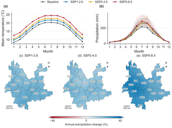
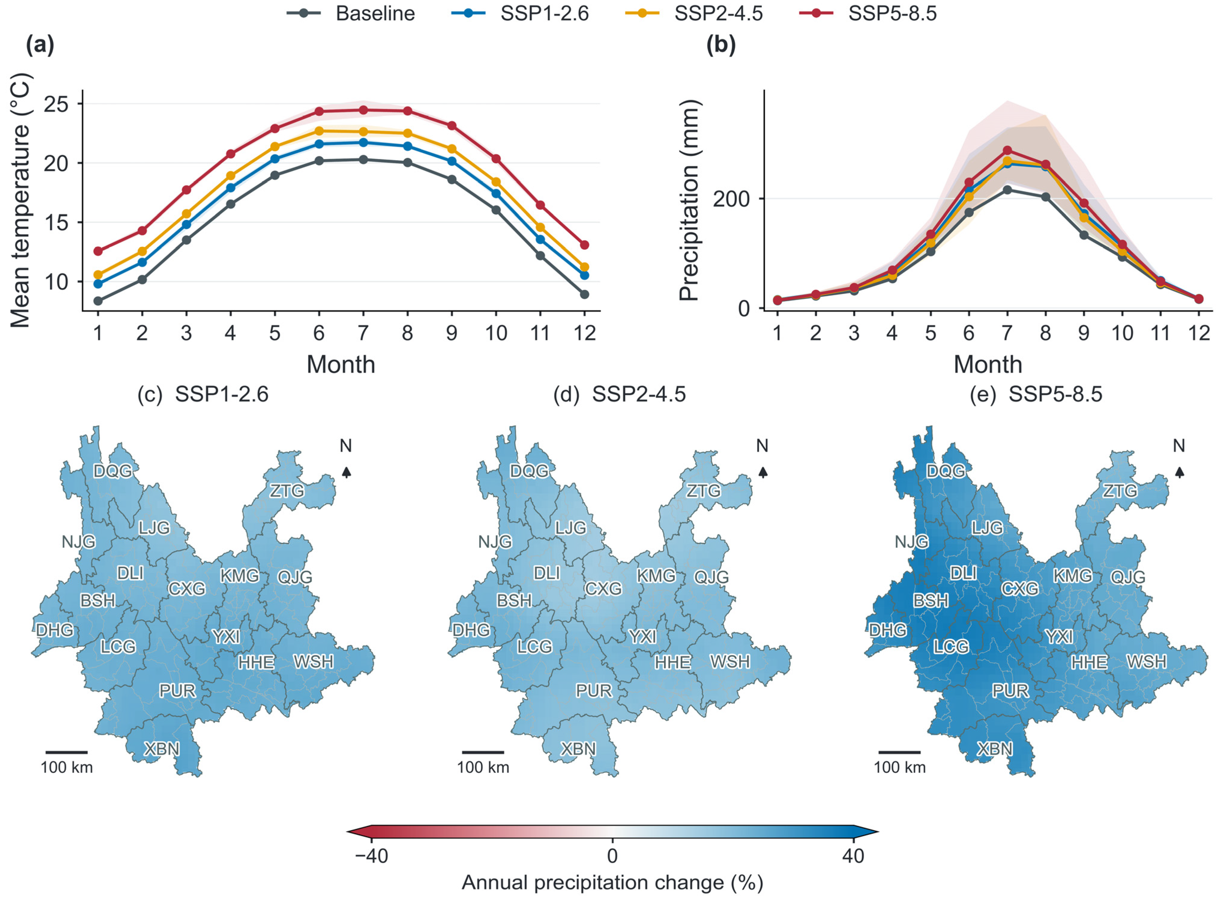
Late-century mean annual warming was 1.43, 2.38, and 4.23 °C under SSP1-2.6, SSP2-4.5, and SSP5-8.5, respectively. Under SSP5-8.5, GCM warming ranged from 3.97 to 4.40 °C and annual precipitation change ranged from +9.6% to +70.2% (mean +30.1%; Figure 10; Table S11). Despite wetter annual conditions, every GCM reduced province-wide dry-season P − ET0 by 20.7–62.8 mm (mean −45.3 mm). Regional mean reductions were 54.1 mm in the Central window, 49.6 mm in the Southeast, and 44.2 mm in the Southwest. Northwest responses crossed zero (−78.2 to +43.7 mm), demonstrating that annual rainfall alone obscures seasonal water constraints.
Figure 10.
Three-GCM monthly climate context at 10 arc min. (a) Temperature and (b) precipitation for baseline and 2081–2100: lines show GCM means, bands show their ranges. (c–e) Annual precipitation changes under SSP1-2.6, SSP2-4.5, and SSP5-8.5. Burgundy denotes decreases and blue denotes increases; end triangles identify values beyond ±40%. Maps use CGCS2000 Albers. Monthly temperature equals (minimum + maximum)/2; water-balance diagnostics are in Table S11.
4. Discussion
4.1. Predictive Reliability and Model Selection
The provincial surveys provided 4281 species–cell records across 119 counties, allowing nine pests to be compared with the same predictors and spatial evaluation design. Ensemble AUC nevertheless ranged from 0.591 to 0.778 (Table 4). P. diminuta had the highest mean AUC but substantial fold variation, whereas the 27-cell H. parallela model was weakly discriminating. Geographic coverage and total record count therefore need to be considered alongside the number of presences in each test fold. Climate-cell deduplication and nested spatial evaluation reduce duplication and selection bias; uneven survey effort remains a source of error [23,24,25,26,27,28,29,30,61].
Ensemble averaging did not outperform every component: mean ANN AUC was 0.729, compared with 0.700 for the ensemble. Including ANN improved ensemble AUC by 0.0165, but SSP5-8.5 area changes also depended strongly on model composition. For A. cinerea, the estimated change was −50.7% with ANN and −91.7% without it (Table S10). These comparisons include the effect of separately selected thresholds. Similar mean ANN performance across initialisations (Table S13) supports numerical repeatability, while the area comparison shows that projection sensitivity persists. Background design also mattered: controlled RF mean AUC ranged from 0.674 with SRE-restricted background to 0.699 with uniform background (Table S3). These results favour reporting component performance and sensitivity alongside the ensemble map.
Recent insect studies provide useful comparisons. Valdés-Díaz et al. [66] combined six algorithms for Aulacaspis yasumatsui and found that predictor selection and algorithm choice strongly affected model performance. Gao et al. [67] used a TSS-weighted ensemble for Rhodnius prolixus, mapped the distribution shape of member predictions using kurtosis, and evaluated predictions against independent field observations. These studies illustrate the value of examining model selection and spatial uncertainty alongside ensemble-mean suitability. In our study, sensitivity analyses assessed how ANN inclusion and background sampling affected predictions, while nested spatial cross-validation evaluated model performance within Yunnan. Future work should incorporate independent field validation and quantify the contributions of algorithms, GCMs, and thresholds to projection uncertainty.
Elevation describes the pronounced terrain gradient in Figure 2b, but its correlation with annual mean temperature (ρ = −0.90) complicates their joint interpretation. Adding elevation changed the controlled RF mean AUC by only 0.0004 across the eight grasshoppers (Table S9). Retaining the scenario-varying temperature predictor therefore kept the primary comparison parsimonious [29]. Terrain effects on radiation, soil moisture, and vegetation remain plausible at finer scales than the climate grid can resolve.
4.2. Species-Specific Climate Responses and Feeding Ecology
Warm-quarter precipitation had the highest permutation importance for six species, whereas bio4, bio1, and bio15 ranked first for A. cinerea, P. japonica, and A. sinensis, respectively (Figure 4). The retained records also sampled different moisture environments: median bio18 was 652 mm for O. chinensis and 408.5 mm for P. diminuta (Figure 3). O. chinensis gained suitable area under SSP1-2.6 and SSP2-4.5, but lost 18.5% under SSP5-8.5; P. diminuta lost 54.6% under the high-emission pathway (Table 5). A shared leading predictor therefore did not imply the same response across climate scenarios. Comparing these responses within one design extends the species-specific perspective of previous grasshopper studies [7,8,9,10,31,32,33,34,35].
The seven acridids and A. sinensis are principally foliage feeders, whereas H. parallela has root-feeding larvae and foliage-feeding adults [39,68,69]. Seasonal moisture may affect foliage-feeding species through plant growth as well as direct insect water balance. For H. parallela, adult collection sites provide limited information about the soil conditions experienced by larvae. Its sparse sample and missing life-stage and soil data justify a separate exploratory interpretation and exclusion from combined revisit rankings. Necrophagy and cannibalism reported in some locusts [70] do not establish that the focal species cease feeding on plants during a drought. Nutritional conditions, temperature, and density can modify feeding behaviour [12,71].
P. japonica combines the strongest grasshopper contraction under late-century SSP5-8.5 (63.4%) with a 139.0 km centroid displacement. Published observations describe one generation per year, adult overwintering, and reproductive diapause [68,72], suggesting seasonal processes worth testing against its temperature association. Two generations have been reported for A. sinensis in Osaka [73], and one for H. parallela in a Chinese study [69]. These records provide biological context without establishing voltinism throughout Yunnan. The present climatic averages cannot distinguish effects on development, winter survival, diapause, or the timing of food availability. Stage-specific observations would help explain why projected responses differ among species [8,10].
4.3. Plant Resources and Climate-Model Uncertainty
Field-associated plant indices added some predictive information: controlled RF mean AUC increased from 0.699 to 0.708–0.715 across the three bandwidths (Table S3). The scale dependence and heterogeneous plant recording limit attribution of this improvement to food resources. The static and climate-conditioned plant comparisons address alternative assumptions about future vegetation (Table S4). Holding plant context constant may miss forage losses or newly suitable resources; recalculating it from climate allows change but shares climatic information with the pest model [35,44,45,46,74]. Neither comparison establishes the added value of independently observed vegetation. An NDVI/EVI test was not included; seasonally matched vegetation measurements would be useful given their role in other grasshopper models [13,33,34]. Gao et al. [67] included vegetation-index variables in an insect ensemble, illustrating a useful comparison for future work rather than evidence that NDVI or EVI would improve the present models.
Monthly diagnostics help interpret the prominence of precipitation predictors. Under late-century SSP5-8.5, annual rainfall increased by a three-GCM mean of 30.1%, while November–April P − ET0 decreased by 45.3 mm (Figure 10; Table S11). Mean dry-season reductions were 54.1 mm in Central Yunnan and 49.6 mm in the Southeast. A wetter annual climate can therefore coincide with greater pre-monsoon climatic water deficit, potentially changing the seasonal availability of green tissue. This is a mechanism to test with plant observations: reference evapotranspiration does not account for rooting depth, soil-water storage, or grazing.
Using three GCMs and four matched periods separates temporal changes from differences among emission pathways. O. chinensis illustrates why the high-emission result should not be generalised to all futures. For G. marmoratus, late-century SSP5-8.5 member areas spanned 1.9–277.3 × 10³ km2 despite a consensus contraction (Table S5). Threshold choice and ANN inclusion added further variation (Tables S5 and S10). Area estimates, centroid intervals, and directional-agreement maps should therefore be interpreted together. The conditional resampling describes variation among fitted folds and GCMs; uncertainty from observation error, dispersal, and future land use remains outside those intervals.
The uncertainty diagnostics address different questions. Kurtosis, as used by Gao et al. [67], describes the shape of the distribution of member predictions; our directional agreement summarises whether algorithm–fold–GCM members predict the same sign of change (Figure S5). Neither measures prediction error against independent observations. Our centroid intervals are conditional on the models fitted within the spatial cross-validation folds and the three GCMs considered, while sensitivity to threshold choice and ANN inclusion was assessed separately. We did not partition total projection uncertainty among algorithms, GCMs, and thresholds or calculate a comparable pixel-level statistic describing the distribution of member predictions. High directional agreement, including consistent projections of habitat contraction, therefore reflects consistency within the evaluated ensemble rather than a complete assessment of predictive uncertainty.
4.4. Implications for Surveillance
The survey rankings and climatic projections serve complementary monitoring purposes. Wuhua, Yuanjiang, and Eshan offer well-documented county-level starting points for revisits, with Xizhu, Manlai, and Fuliangpeng leading the township list (Figure 7). Both top-ten sets were unchanged across the tested index weights (Table S7), although uneven effort can favour frequently surveyed units. Additional sites could be selected at projected margins and in poorly sampled or low-agreement areas, with site locations checked against actual grassland cover. This would allow existing field teams to retain continuity while testing where suitability is changing. H. parallela warrants a separate soil- and life-stage-specific survey.
The 2.5 arc min climate grid covers approximately 4.2 × 4.6 km at 25° N. Administrative boundaries help locate monitoring units but do not resolve within-cell terrain or vegetation. Area totals cover the provincial mask, and centroid movements summarise changing suitability without modelling colonisation. Relating recent observations to 1970–2000 climate normals also limits interpretation of survey-year conditions. Repeat visits should record non-detections, effort, weather, life stage, vegetation, soil, and voucher information so that detection can be estimated in a hierarchical analysis [75]. Such repeat histories were unavailable in the present archive. Performance was evaluated within Yunnan; independent surveys in other regions or years remain necessary to assess transferability.
5. Conclusions
The provincial census and special survey provided a common evidence base for comparing nine grassland insect pests across Yunnan. After climate-grid filtering, 4281 species–cell records were analysed with five climatic predictors and a ten-algorithm, TSS-weighted ensemble under nested spatial cross-validation. Ensemble AUC ranged from 0.591 to 0.778 and TSS from 0.198 to 0.365. Warm-quarter precipitation had the highest permutation importance for six species, whereas temperature seasonality, annual mean temperature, and precipitation seasonality led for A. cinerea, P. japonica, and A. sinensis, respectively. The results indicate species-specific climatic associations; the 27-cell H. parallela model remains exploratory.
Projections from three GCMs across four periods from 2021 to 2100 differentiated responses to the three emission pathways. O. chinensis had the largest baseline threshold-defined suitable area (235.3 × 10³ km2); its late-century area increased by 9.0% under SSP1-2.6 and 12.0% under SSP2-4.5, but decreased by 18.5% under SSP5-8.5. Under SSP5-8.5, late-century consensus suitable area contracted for all eight grasshopper species, including decreases of 63.4% for P. japonica and 54.6% for P. diminuta. Their species-level responses across periods were not uniformly progressive. Late-century centroid displacement among the grasshoppers ranged from 31.6 to 139.0 km, with substantial variation among fitted folds and climate models.
The combined analysis distinguishes projected climatic change from survey-based revisit priorities. Wuhua District in Kunming and Yuanjiang and Eshan counties in Yuxi ranked highest for county-level revisits; Xizhu, Manlai, and Fuliangpeng ranked highest among townships. These established survey locations provide starting points for coordinated monitoring, while species-specific maps identify areas of projected change for additional sampling. The results support species-specific surveillance, early warning, and repeated monitoring at current cores and climate-sensitive margins.
Supplementary Materials
The following supporting information can be downloaded at: https://www.mdpi.com/article/10.3390/insects17101028/s1. Table S1: Species and algorithm performance; Table S2: Collinearity diagnostics; Table S3: Controlled RF sensitivity; Table S4: Static and climate-conditioned plant sensitivity; Table S5: Threshold sensitivity and member dispersion, including member dispersion under SSP5-8.5; Table S6: Conditional centroid displacement intervals; Table S7: Revisit-index weight sensitivity; Table S8: Taxonomy and biological interpretation; Table S9: Occurrence elevation and controlled DEM sensitivity; Table S10: Algorithm inclusion and class weighting, including projection sensitivity to ANN inclusion; Table S11: Seasonal climate changes under SSP1-2.6, SSP2-4.5, and SSP5-8.5; Table S12a: All-period suitable area and centroid displacement for Acrida cinerea; Table S12b: All-period suitable area and centroid displacement for Gastrimargus marmoratus; Table S12c: All-period suitable area and centroid displacement for Oxya chinensis; Table S12d: All-period suitable area and centroid displacement for Patanga japonica; Table S12e: All-period suitable area and centroid displacement for Phlaeoba infumata; Table S12f: All-period suitable area and centroid displacement for Trilophidia annulata; Table S12g: All-period suitable area and centroid displacement for Atractomorpha sinensis; Table S12h: All-period suitable area and centroid displacement for Holotrichia parallela; Table S12i: All-period suitable area and centroid displacement for Pseudoxya diminuta; Table S13a: ANN structure selection and ensemble weights; Table S13b: ANN sensitivity to fixed alternative initializations; Figure S1: Consensus relative-suitability change under SSP1-2.6 for 2081–2100; Figure S2: Consensus relative-suitability change under SSP2-4.5 for 2081–2100; Figure S3: Consensus suitable-area change across four 20-year periods; Figure S4: Consensus centroid displacement from baseline across four 20-year periods; Figure S5: Weighted agreement in the direction of suitability change under SSP5-8.5 for 2081–2100.
Author Contributions
Conceptualisation, Y.L. and X.C. (Xiaoxue Chen); Methodology, Y.L. and Q.J.; Software, Y.L.; Validation, Y.L., Q.J., X.C. (Xiaoxue Chen), L.G., and X.C. (Xinqiang Chen); Formal Analysis, Y.L. and Q.J.; Investigation, X.C. (Xiaoxue Chen), L.G., X.C. (Xinqiang Chen), S.H., and T.P.; Resources, X.C. (Xinqiang Chen) and X.C. (Xiaoxue Chen); Data Curation, X.C. (Xiaoxue Chen), L.G., and X.C. (Xinqiang Chen); Writing—Original Draft Preparation, Y.L.; Writing—Review and Editing, all authors; Visualisation, Y.L.; Supervision, Y.L.; Project Administration, X.C. (Xiaoxue Chen). All authors have read and agreed to the published version of the manuscript.
Funding
This study was supported by Yunnan Fundamental Research Projects (grant no. 202601CI070005).
Institutional Review Board Statement
Not applicable. The study used field observations and records of non-protected invertebrates and did not involve humans or vertebrate animals.
Informed Consent Statement
Not applicable.
Data Availability Statement
Processed occurrences, climate values, folds, tuning and evaluation outputs, weights, permutation replicates, scenario summaries, and scripts are included in the revision archive. Raw field tables are held by the Yunnan Institute of Forest Inventory and Planning under its data-access procedures. WorldClim source URLs (https://www.worldclim.org/) and regional crop checksums are archived; GBIF access is described in Section 2.2.3.
Acknowledgements
The authors thank prefectural and county forestry and grassland personnel who completed the field programmes and the taxonomic experts who reviewed specimens and database determinations. The authors also thank all staff of the Pest Research Center of the Yinglin Branch for their dedication and contributions to this project.
Conflicts of Interest
The authors declare no conflicts of interest.
References
- Skendžić, S.; Zovko, M.; Pajač Živković, I.; Lešić, V.; Lemić, D. The impact of climate change on agricultural insect pests. Insects 2021, 12, 440. [Google Scholar] [CrossRef] [Scilit]
- Lehmann, P.; Ammunét, T.; Barton, M.; Battisti, A.; Eigenbrode, S.D.; Jepsen, J.U.; Kalinkat, G.; Neuvonen, S.; Niemelä, P.; Terblanche, J.S.; et al. Complex responses of global insect pests to climate warming. Front. Ecol. Environ. 2020, 18, 141–150. [Google Scholar] [CrossRef] [Scilit]
- Subedi, B.; Poudel, A.; Aryal, S. The impact of climate change on insect pest biology and ecology: Implications for pest management strategies, crop production, and food security. J. Agric. Food Res. 2023, 14, 100733. [Google Scholar] [CrossRef] [Scilit]
- Deutsch, C.A.; Tewksbury, J.J.; Huey, R.B.; Sheldon, K.S.; Ghalambor, C.K.; Haak, D.C.; Martin, P.R. Impacts of climate warming on terrestrial ectotherms across latitude. Proc. Natl. Acad. Sci. USA 2008, 105, 6668–6672. [Google Scholar] [CrossRef] [Scilit]
- Chen, I.C.; Hill, J.K.; Ohlemüller, R.; Roy, D.B.; Thomas, C.D. Rapid range shifts of species associated with high levels of climate warming. Science 2011, 333, 1024–1026. [Google Scholar] [CrossRef] [Scilit]
- Bebber, D.P.; Ramotowski, M.A.T.; Gurr, S.J. Crop pests and pathogens move polewards in a warming world. Nat. Clim. Change 2013, 3, 985–988. [Google Scholar] [CrossRef] [Scilit]
- Fartmann, T.; Poniatowski, D.; Holtmann, L. Habitat availability and climate warming drive changes in the distribution of grassland grasshoppers. Agric. Ecosyst. Environ. 2021, 320, 107565. [Google Scholar] [CrossRef] [Scilit]
- Lemoine, N.P. Phenology dictates the impact of climate change on geographic distributions of six co-occurring North American grasshoppers. Ecol. Evol. 2021, 11, 18575–18590. [Google Scholar] [CrossRef] [Scilit]
- Koot, E.M.; Morgan-Richards, M.; Trewick, S.A. Climate change and alpine-adapted insects: Modelling environmental envelopes of a grasshopper radiation. R. Soc. Open Sci. 2022, 9, 211596. [Google Scholar] [CrossRef] [Scilit]
- Buckley, L.B.; Graham, S.I.; Nufio, C.R. Grasshopper species’ seasonal timing underlies shifts in phenological overlap in response to climate gradients, variability and change. J. Anim. Ecol. 2021, 90, 1252–1263. [Google Scholar] [CrossRef] [Scilit]
- Tian, H.; Stige, L.C.; Cazelles, B.; Kausrud, K.L.; Svarverud, R.; Stenseth, N.C.; Zhang, Z. Reconstruction of a 1910-y-long locust series reveals consistent associations with climate fluctuations in China. Proc. Natl. Acad. Sci. USA 2011, 108, 14521–14526. [Google Scholar] [CrossRef] [Scilit]
- Cease, A.J.; Elser, J.J.; Ford, C.F.; Hao, S.; Kang, L.; Harrison, J.F. Heavy livestock grazing promotes locust outbreaks by lowering plant nitrogen content. Science 2012, 335, 467–469. [Google Scholar] [CrossRef] [Scilit]
- Klein, I.; Oppelt, N.; Kuenzer, C. Application of remote sensing data for locust research and management: A review. Insects 2021, 12, 233. [Google Scholar] [CrossRef] [Scilit]
- Cressman, K. Role of remote sensing in desert locust early warning. J. Appl. Remote Sens. 2013, 7, 075098. [Google Scholar] [CrossRef] [Scilit]
- Kistner-Thomas, E.; Kumar, S.; Jech, L.; Woller, D.A. Modeling rangeland grasshopper (Orthoptera: Acrididae) population density using a landscape-level predictive mapping approach. J. Econ. Entomol. 2021, 114, 1557–1567. [Google Scholar] [CrossRef] [Scilit]
- Elith, J.; Leathwick, J.R. Species distribution models: Ecological explanation and prediction across space and time. Annu. Rev. Ecol. Evol. Syst. 2009, 40, 677–697. [Google Scholar] [CrossRef] [Scilit]
- Guisan, A.; Thuiller, W. Predicting species distribution: Offering more than simple habitat models. Ecol. Lett. 2005, 8, 993–1009. [Google Scholar] [CrossRef] [Scilit]
- Franklin, J. Mapping Species Distributions: Spatial Inference and Prediction; Cambridge University Press: Cambridge, UK, 2009. [Google Scholar]
- Peterson, A.T.; Soberón, J.; Pearson, R.G.; Anderson, R.P.; Martínez-Meyer, E.; Nakamura, M.; Araújo, M.B. Ecological Niches and Geographic Distributions; Princeton University Press: Princeton, NJ, USA, 2011. [Google Scholar]
- Araújo, M.B.; New, M. Ensemble forecasting of species distributions. Trends Ecol. Evol. 2007, 22, 42–47. [Google Scholar] [CrossRef] [Scilit]
- Thuiller, W. BIOMOD-optimizing predictions of species distributions and projecting potential future shifts under global change. Glob. Change Biol. 2003, 9, 1353–1362. [Google Scholar] [CrossRef] [Scilit]
- Thuiller, W.; Lafourcade, B.; Engler, R.; Araújo, M.B. BIOMOD-a platform for ensemble forecasting of species distributions. Ecography 2009, 32, 369–373. [Google Scholar] [CrossRef] [Scilit]
- Zurell, D.; Franklin, J.; König, C.; Bouchet, P.J.; Dormann, C.F.; Elith, J.; Fandos, G.; Feng, X.; Guillera-Arroita, G.; Guisan, A.; et al. A standard protocol for reporting species distribution models. Ecography 2020, 43, 1261–1277. [Google Scholar] [CrossRef] [Scilit]
- Guillera-Arroita, G.; Lahoz-Monfort, J.J.; Elith, J.; Gordon, A.; Kujala, H.; Lentini, P.E.; McCarthy, M.A.; Tingley, R.; Wintle, B.A. Is my species distribution model fit for purpose? Matching data and models to applications. Glob. Ecol. Biogeogr. 2015, 24, 276–292. [Google Scholar] [CrossRef] [Scilit]
- Roberts, D.R.; Bahn, V.; Ciuti, S.; Boyce, M.S.; Elith, J.; Guillera-Arroita, G.; Hauenstein, S.; Lahoz-Monfort, J.J.; Schröder, B.; Thuiller, W.; et al. Cross-validation strategies for data with temporal, spatial, hierarchical, or phylogenetic structure. Ecography 2017, 40, 913–929. [Google Scholar] [CrossRef] [Scilit]
- Valavi, R.; Elith, J.; Lahoz-Monfort, J.J.; Guillera-Arroita, G. blockCV: An R package for generating spatially or environmentally separated folds for k-fold cross-validation of species distribution models. Methods Ecol. Evol. 2019, 10, 225–232. [Google Scholar] [CrossRef] [Scilit]
- Barbet-Massin, M.; Jiguet, F.; Albert, C.H.; Thuiller, W. Selecting pseudo-absences for species distribution models: How, where and how many? Methods Ecol. Evol. 2012, 3, 327–338. [Google Scholar] [CrossRef] [Scilit]
- Fourcade, Y.; Engler, J.O.; Rödder, D.; Secondi, J. Mapping species distributions with MaxEnt using a geographically biased sample of presence data: A performance assessment of methods for correcting sampling bias. PLoS ONE 2014, 9, e97122. [Google Scholar] [CrossRef] [Scilit]
- Dormann, C.F.; Elith, J.; Bacher, S.; Buchmann, C.; Carl, G.; Carré, G.; Marquez, J.R.G.; Gruber, B.; Lafourcade, B.; Leitão, P.J.; et al. Collinearity: A review of methods to deal with it and a simulation study evaluating their performance. Ecography 2013, 36, 27–46. [Google Scholar] [CrossRef] [Scilit]
- Sillero, N.; Barbosa, A.M. Common mistakes in ecological niche models. Int. J. Geogr. Inf. Sci. 2021, 35, 213–226. [Google Scholar] [CrossRef] [Scilit]
- Li, J.X.; Shao, L.; Guan, T.X.; Huang, J.J.; Jin, Q.; Biyake, D.; Ren, J.L.; Zhao, L. Analysis of potential suitable habitats of six dominant locusts in the Bortala Mongol Autonomous Prefecture, Xinjiang based on the MaxEnt model. Chin. J. Grassl. 2024, 46, 101–111. (In Chinese) [Google Scholar]
- Li, D.; Gan, H.; Li, X.; Zhou, H.; Zhang, H.; Liu, Y.; Dong, R.; Hua, L.; Hu, G. Changes in the range of four advantageous grasshopper habitats in the Hexi Corridor under future climate conditions. Insects 2024, 15, 243. [Google Scholar] [CrossRef] [Scilit]
- Du, B.; Wei, J.; Lin, K.; Lu, L.; Ding, X.; Ye, H.; Huang, W.; Wang, N. Spatial and temporal variability of grassland grasshopper habitat suitability and its main influencing factors. Remote Sens. 2022, 14, 3910. [Google Scholar] [CrossRef] [Scilit]
- Ahmed, R.; Huang, W.; Dong, Y.; Dildar, Z.; Ashraf, H.A.; Rahman, Z.U.; Rysbekova, A. Integrating remote sensing, machine learning, and degree-day models for predicting grasshopper habitat suitability in temperate grasslands. Remote Sens. 2025, 17, 3955. [Google Scholar] [CrossRef] [Scilit]
- Guo, J.; Huang, W.; Dong, Y.; Xie, Q.; Fang, G.; Yue, F.; Wang, K.; Hao, Z.; Zhang, Y.; Cheng, X.; et al. Spatiotemporal dynamics of grasshopper habitats under future climate projections, vegetation growth, and land use change. Int. J. Appl. Earth Obs. Geoinf. 2026, 152, 105481. [Google Scholar] [CrossRef] [Scilit]
- Sofaer, H.R.; Jarnevich, C.S.; Pearse, I.S.; Smyth, R.L.; Auer, S.; Cook, G.L.; Edwards, T.C.; Guala, G.F.; Howard, T.G.; Morisette, J.T.; et al. Development and delivery of species distribution models to inform decision-making. BioScience 2019, 69, 544–557. [Google Scholar] [CrossRef] [Scilit]
- Yunnan Forestry and Grassland Administration. Report on the Results of the Grassland Pest Census in Yunnan Province; Technical Report; Yunnan Forestry and Grassland Administration: Kunming, China, 2024. (In Chinese)
- Yunnan Forestry and Grassland Pest Control and Quarantine Bureau; Yinglin Branch, Yunnan Institute of Forest Inventory and Planning. Special Survey Report on Grassland Grasshoppers in Yunnan Province; Technical Report; Yunnan Forestry and Grassland Pest Control and Quarantine Bureau: Kunming, China, 2025. (In Chinese)
- Mao, B.Y.; Ren, G.D.; Ou, X.H. Fauna, Distribution Pattern and Adaptability of Acridoidea from Yunnan; China Forestry Publishing House: Beijing, China, 2011. (In Chinese) [Google Scholar]
- Pedregosa, F.; Varoquaux, G.; Gramfort, A.; Michel, V.; Thirion, B.; Grisel, O.; Blondel, M.; Prettenhofer, P.; Weiss, R.; Dubourg, V.; et al. Scikit-learn: Machine learning in Python. J. Mach. Learn. Res. 2011, 12, 2825–2830. Available online: https://www.jmlr.org/papers/v12/pedregosa11a.html (accessed on 25 July 2026).
- NY/T 1578-2007; Specification for Grassland Grasshopper Survey. Ministry of Agriculture: Beijing, China, 2007. (In Chinese)
- GB/T 25875-2010; Guideline for Segmentating and Monitoring the Inhabitable Area of Locust and Grasshopper in Grassland. General Administration of Quality Supervision, Inspection and Quarantine; Standardization Administration of China: Beijing, China, 2011. (In Chinese)
- GBIF Occurrence Download. Available online: https://www.gbif.org/ (accessed on 4 July 2026).
- Araújo, M.B.; Luoto, M. The importance of biotic interactions for modelling species distributions under climate change. Glob. Ecol. Biogeogr. 2007, 16, 743–753. [Google Scholar] [CrossRef] [Scilit]
- Kissling, W.D.; Dormann, C.F.; Groeneveld, J.; Hickler, T.; Kühn, I.; McInerny, G.J.; Montoya, J.M.; Römermann, C.; Schiffers, K.; Schurr, F.M.; et al. Towards novel approaches to modelling biotic interactions in multispecies assemblages at large spatial extents. J. Biogeogr. 2012, 39, 2163–2178. [Google Scholar] [CrossRef] [Scilit]
- Wisz, M.S.; Pottier, J.; Kissling, W.D.; Pellissier, L.; Lenoir, J.; Damgaard, C.F.; Dormann, C.F.; Forchhammer, M.C.; Grytnes, J.A.; Guisan, A.; et al. The role of biotic interactions in shaping distributions and realised assemblages of species: Implications for species distribution modelling. Biol. Rev. 2013, 88, 15–30. [Google Scholar] [CrossRef] [Scilit]
- Hijmans, R.J.; Cameron, S.E.; Parra, J.L.; Jones, P.G.; Jarvis, A. Very high resolution interpolated climate surfaces for global land areas. Int. J. Climatol. 2005, 25, 1965–1978. [Google Scholar] [CrossRef] [Scilit]
- Fick, S.E.; Hijmans, R.J. WorldClim 2: New 1-km spatial resolution climate surfaces for global land areas. Int. J. Climatol. 2017, 37, 4302–4315. [Google Scholar] [CrossRef] [Scilit]
- Allen, R.G.; Pereira, L.S.; Raes, D.; Smith, M. Crop Evapotranspiration: Guidelines for Computing Crop Water Requirements; FAO Irrigation and Drainage Paper 56; FAO: Rome, Italy, 1998; Available online: https://www.fao.org/4/x0490e/x0490e00.htm (accessed on 23 September 2026).
- Meynard, C.N.; Gay, P.E.; Lecoq, M.; Foucart, A.; Piou, C.; Chapuis, M.P. Climate-driven geographic distribution of the desert locust during recession periods: Subspecies’ niche differentiation and relative risks under scenarios of climate change. Glob. Change Biol. 2017, 23, 4739–4749. [Google Scholar] [CrossRef] [Scilit]
- Guan, J.; Li, M.; Ju, X.; Lin, J.; Wu, J.; Zheng, J. The potential habitat of desert locusts is contracting: Predictions under climate change scenarios. PeerJ 2021, 9, e12311. [Google Scholar] [CrossRef] [Scilit]
- Lv, Y.Y.; Yu, H.Y.; Chen, W.; Li, M.; Yi, S.H.; Meng, B.P. Predicting inhabitable areas for locust based on field observation and multi-environmental factors in alpine grassland: A case study in the Qilian Mountain National Park, China. Front. Ecol. Evol. 2023, 11, 1149952. [Google Scholar] [CrossRef] [Scilit]
- Sun, Z.X.; Hu, Z.X.; Ye, H.C.; Huang, W.J.; Qimuge, E.; Zhang, Y. Application of MaxEnt and remote sensing technology in grassland locust disaster risk monitoring: An example from the agricultural heritage systems of East Ujimqin Banner. J. Ecol. Rural Environ. 2022, 38, 1265–1272. (In Chinese) [Google Scholar] [CrossRef]
- Wang, Q.; Ta, F.; Yue, F.; Ma, H.; Yang, D. Potential distribution and key factors of Dasyhippus barbipes (Orthoptera: Acrididae: Gomphocerinae) in China under climate change scenarios. Insects 2026, 17, 616. [Google Scholar] [CrossRef] [Scilit]
- Phillips, S.J.; Anderson, R.P.; Schapire, R.E. Maximum entropy modeling of species geographic distributions. Ecol. Model. 2006, 190, 231–259. [Google Scholar] [CrossRef] [Scilit]
- Phillips, S.J.; Dudík, M. Modeling of species distributions with Maxent: New extensions and a comprehensive evaluation. Ecography 2008, 31, 161–175. [Google Scholar] [CrossRef] [Scilit]
- Merow, C.; Smith, M.J.; Silander, J.A. A practical guide to MaxEnt for modeling species’ distributions: What it does, and why inputs and settings matter. Ecography 2013, 36, 1058–1069. [Google Scholar] [CrossRef] [Scilit]
- Breiman, L. Random forests. Mach. Learn. 2001, 45, 5–32. [Google Scholar] [CrossRef] [Scilit]
- Friedman, J.H. Greedy function approximation: A gradient boosting machine. Ann. Stat. 2001, 29, 1189–1232. [Google Scholar] [CrossRef] [Scilit]
- Elith, J.; Leathwick, J.R.; Hastie, T. A working guide to boosted regression trees. J. Anim. Ecol. 2008, 77, 802–813. [Google Scholar] [CrossRef] [Scilit]
- Cawley, G.C.; Talbot, N.L.C. On over-fitting in model selection and subsequent selection bias in performance evaluation. J. Mach. Learn. Res. 2010, 11, 2079–2107. Available online: https://www.jmlr.org/papers/v11/cawley10a.html (accessed on 25 July 2026).
- Fielding, A.H.; Bell, J.F. A review of methods for the assessment of prediction errors in conservation presence/absence models. Environ. Conserv. 1997, 24, 38–49. [Google Scholar] [CrossRef] [Scilit]
- Allouche, O.; Tsoar, A.; Kadmon, R. Assessing the accuracy of species distribution models: Prevalence, kappa and the true skill statistic (TSS). J. Appl. Ecol. 2006, 43, 1223–1232. [Google Scholar] [CrossRef] [Scilit]
- Liu, C.; Berry, P.M.; Dawson, T.P.; Pearson, R.G. Selecting thresholds of occurrence in the prediction of species distributions. Ecography 2005, 28, 385–393. [Google Scholar] [CrossRef] [Scilit]
- Liu, C.; Newell, G.; White, M. On the selection of thresholds for predicting species occurrence with presence-only data. Ecol. Evol. 2016, 6, 337–348. [Google Scholar] [CrossRef] [Scilit]
- Valdés-Díaz, S.; Tuñón, R.; Castillo, D.; Sanchez, A.; Virola-Vasquez, B.; Corro, P.E.; Serrano-Peraza, F.; Zachrisson, B.; Loaiza, J.; Chang, R.; et al. Ensemble distribution modeling of the globally invasive Asian cycad scale, Aulacaspis yasumatsui Takagi, 1977 (Hemiptera: Diaspididae). Insects 2025, 16, 1016. [Google Scholar] [CrossRef] [Scilit]
- Gao, Y.; Añez, N.; Chaves, L.F. High spatial resolution ensemble species distribution modeling of Rhodnius prolixus, vector of Chagas disease, in western Venezuela. GeoHealth 2026, 10, e2025GH001628. [Google Scholar] [CrossRef] [Scilit]
- Tanaka, S. Biology of Patanga japonica (Orthoptera, Acrididae): Nymphal growth, host plants, reproductive activity, hatching behavior, and adult morphology. J. Orthoptera Res. 2023, 32, 93–108. [Google Scholar] [CrossRef] [Scilit]
- Zhang, H.; Teng, X.; Luo, Q.; Sheng, Z.; Guo, X.; Wang, G.; Li, W.; Yuan, G. Flight and walking performance of dark black chafer beetle Holotrichia parallela (Coleoptera: Scarabaeidae) in the presence of known hosts and attractive nonhost plants. J. Insect Sci. 2019, 19, 14. [Google Scholar] [CrossRef] [Scilit]
- Bazazi, S.; Buhl, C.; Hale, J.J.; Anstey, M.L.; Sword, G.A.; Simpson, S.J.; Couzin, I.D. Collective motion and cannibalism in locust migratory bands. Curr. Biol. 2008, 18, 735–739. [Google Scholar] [CrossRef] [Scilit]
- Youngblood, J.P.; Cease, A.J.; Talal, S.; Copa, F.; Medina, H.E.; Rojas, J.E.; Trumper, E.V.; Angilletta, M.J., Jr.; Harrison, J.F. Climate change expected to improve digestive rate and trigger range expansion in outbreaking locusts. Ecol. Monogr. 2023, 93, e1550. [Google Scholar] [CrossRef] [Scilit]
- Tanaka, S. Temperature-dependent phototaxis in overwintering adults of the grasshopper Patanga japonica (Orthoptera, Acrididae). J. Orthoptera Res. 2024, 33, 71–86. [Google Scholar] [CrossRef] [Scilit]
- Sasaki, K.; Akao, R.; Ueda, S.; Hirai, R.; Hirai, N. Life history characteristics and changes in distribution of the alien grasshopper Atractomorpha sinensis in Osaka Prefecture, Japan. Annu. Rep. Kansai Plant Prot. Soc. 2025, 67, 81–86. [Google Scholar] [CrossRef] [Scilit]
- Araújo, M.B.; Peterson, A.T. Uses and misuses of bioclimatic envelope modeling. Ecology 2012, 93, 1527–1539. [Google Scholar] [CrossRef] [Scilit]
- Fiske, I.; Chandler, R. unmarked: An R package for fitting hierarchical models of wildlife occurrence and abundance. J. Stat. Softw. 2011, 43, 1–23. [Google Scholar] [CrossRef] [Scilit]

Disclaimer/Publisher’s Note: The statements, opinions and data contained in all publications are solely those of the individual author(s) and contributor(s) and not of MDPI and/or the editor(s). MDPI and/or the editor(s) disclaim responsibility for any injury to people or property resulting from any ideas, methods, instructions or products referred to in the content. |
© 2026 by the authors. Licensee MDPI, Basel, Switzerland. This article is an open access article distributed under the terms and conditions of the Creative Commons Attribution (CC BY) license.