SPH-Based Local Lubricant Availability Assessment and Candidate-Region Screening for Oil Suction Port Placement Under Continuous Maneuvering

Abstract

In aviation lubrication systems, changes in lubricant flow and spatial distribution under different operating conditions can affect lubricant delivery and lubrication performance. Existing studies have used flow variables such as velocity and pressure, together with instantaneous spatial distributions, to characterize flow states. Although these quantities can effectively characterize flow states and their evolution, they are often difficult to directly translate into quantitative evaluation results for structural design, comparison of different configurations, and engineering decision-making. To address this issue, a local lubricant availability assessment and candidate-region screening approach is developed based on smoothed particle hydrodynamics (SPH) simulation results. Low-percentile availability A₅, minimum availability A_min, and the longest continuous low-oil duration L₅₀ are jointly used to assess the local lubricant state at different spatial locations. An aviation lubricant tank is considered as the application case, and local lubricant conditions under different initial oil volumes and baffle configurations are compared under identical maneuvering conditions. The results show that, within the investigated volume range, the initial oil volume is closely related to the local lubricant state and the extent of the candidate region. As the oil volume decreases, local lubricant deficiency becomes more pronounced, and the differences among baffle configurations become more evident. At an initial oil volume of 10 L, the cross-baffle configuration provides the largest candidate-region area ratio among the four configurations, reaching 59.39%, compared with 4.19% for the no-baffle case. The proposed framework translates transient flow differences under different operating conditions and structural configurations into spatially explicit candidate regions, providing a quantitative basis for preliminary oil suction port placement.

1. Introduction

Aviation transmission lubrication systems are subjected to complex motions involving attitude changes, acceleration and deceleration, and rotation. Continuous changes in inertial effects during operation can induce pronounced free-surface motion and spatial redistribution of lubricant within the cavity [1]. In practical lubrication systems, lubricant must continuously migrate through complex internal structures and reach the required functional regions. Its spatial distribution changes with operating conditions, and local accumulation or reduction in lubricant content, together with changes in supply pathways, may affect lubricant delivery to critical regions [1,2,3]. Recent studies have investigated maneuver-induced liquid motion and wall loads in aircraft fuel tanks [4], as well as oil–air mixing and separation in automotive lubricant tanks under racetrack maneuvers [5]. Constantin et al. combined experiments on a scaled wing-tank model with numerical simulations to examine the additional damping caused by liquid sloshing [6]. For lubricant tanks that supply a lubrication circuit through a local suction port, the lubricant state near potential suction locations therefore needs to be assessed throughout continuous maneuvering. The initial oil volume and internal baffle arrangement also influence liquid migration and spatial distribution. Erzan Topçu and Kılıç compared sloshing in a three-dimensional prismatic tank under different filling ratios, baffle types, excitation amplitudes, and liquid properties [7]. Al-Yacouby and Ahmed examined the effects of perforated and imperforate baffles on sloshing pressure [8], while Wang et al. combined scaled experiments and volume-of-fluid (VOF) simulations to compare the sloshing suppression achieved by different baffle configurations in a tank vehicle [9]. Baffle orientation and excitation mode also affect sloshing suppression. Lu and Cao experimentally investigated the influence of vertical-baffle orientation on resonant wave response and damping [10]. Rubesh Raja V. and Palanisamy used the VOF method to study wave baffles under combined surge and pitch excitation, considering the effects of wave amplitude and the number of periods in the baffle geometry [11]. These studies mainly assessed structural effects through free-surface response, sloshing loads, and damping; the placement analysis of aviation lubricant tanks additionally requires attention to local lubricant conditions during continuous attitude transitions.

Existing studies on transient fluid transport and spatial redistribution have primarily characterized flow behavior through conventional field variables and global performance parameters. In lubrication systems, oil distribution, velocity fields, local flow rates, and churning losses are frequently applied to assess lubricant migration and lubrication performance under variations in rotational speed, motion direction, and dynamic attitude [1,2,3]. Recent studies have also evaluated the oil quantity near specified gears and bearings [2], the wetted proportion of critical components [3], and the flow-rate histories of a predefined suction pipe [12]. Wang et al. used the moving particle semi-implicit (MPS) method to investigate gearbox flow under combined splash and jet lubrication, assessing lubrication through the oil quantity in bearing regions and oil coverage on critical component surfaces [13]. Such local statistics provide a basis for comparing lubricant conditions near specified components. These quantities provide detailed descriptions of transient flow behavior and are effective for mechanism interpretation and comparative evaluation of predefined structures or operating conditions. However, comparisons among multiple potential suction port locations require a consistent spatial assessment that accounts for local lubricant availability, instantaneous depletion, and the duration of low-oil conditions throughout the maneuver. Therefore, further processing of transient flow results is required when the objective shifts from flow-state characterization to spatial layout design.

Numerical simulation has become an important tool for capturing the continuous evolution of fluid flow and spatial distribution under different operating conditions. Mesh-based numerical methods, including the finite volume method, finite element method, and finite difference method, have developed into mature solution frameworks and are commonly combined with interface-capturing approaches such as the volume-of-fluid (VOF) and level-set methods for free-surface tracking and evolution analysis [14,15]. These methods have been widely applied to multiphase and free-surface flows. For liquid sloshing, Mahfoze et al. used the VOF method to compare the dissipation predicted by different turbulence-modeling approaches against experimental measurements [16]. However, for computational domains involving complex internal geometries, moving boundaries, and large-scale liquid migration, mesh generation, moving-boundary treatment, and free-surface/interface tracking can substantially increase the complexity of model construction and numerical solution [17,18,19,20,21]. Smoothed particle hydrodynamics (SPH) employs a fully Lagrangian mesh-free discretization, in which the continuum is represented by computational particles that move with the fluid. Because no conventional volumetric mesh is required for the fluid domain and the free surface can evolve naturally with particle motion, SPH is well suited to problems involving complex geometries, moving boundaries, and substantial free-surface deformation [17,18,19,20,21]. In addition, the local interaction pattern of SPH is well suited to parallel computation, and GPU-accelerated implementations have substantially improved the computational efficiency of large-scale particle simulations [22]. More importantly, Lagrangian particles retain the time histories of their positions and associated physical states throughout the calculation. In recent years, SPH has also been applied to gearbox lubrication and flow simulations involving complex moving boundaries [2,3,23]. For tank sloshing, Sun et al. used MPS to calculate sloshing forces in complex ship tanks under rolling excitation, examining the effects of roll angle and period [24]. Lu and Cao used SPH to compare free-surface elevation, wall pressure, and energy dissipation for different numbers of vertical baffles under varying excitation frequencies and amplitudes [25]. SPH therefore provides not only a means of describing transient flow under complex operating conditions, but also continuous particle-position information that facilitates further quantitative analysis of fluid spatial distributions.

Accordingly, the present study considers an aviation lubricant tank under complex motion and develops an SPH-based post-processing and screening framework that converts transient particle distributions into quantitative descriptors of local lubricant availability and spatial candidate regions for oil suction port placement. Regularly arranged virtual sampling domains extract local lubricant-availability histories from the particle data. Low-percentile availability A₅, minimum availability A_min, and the longest continuous low-oil duration L₅₀ describe the overall level, extreme depletion, and persistence of low-oil conditions, respectively. Stage-wise A₅ is combined with A_min and L₅₀ over the complete maneuvering period to identify candidate locations and compare the effects of initial oil volume and baffle configuration. The resulting regions provide a quantitative reference for preliminary oil suction port placement.

2. Materials and Methods

2.1. Characterization of Local Lubricant Availability

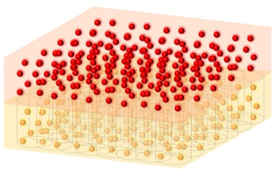
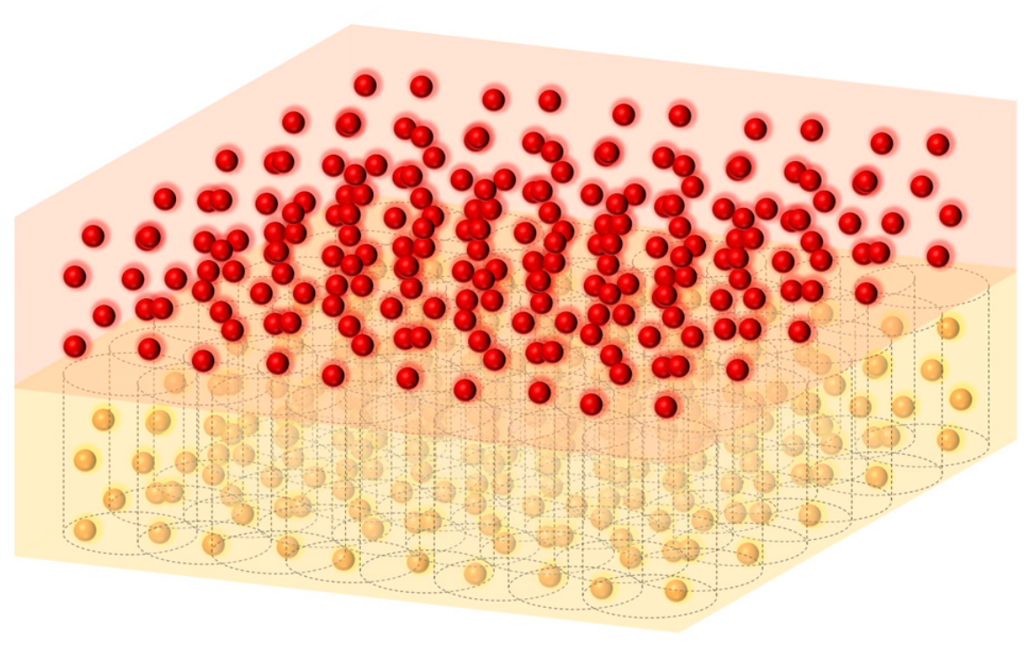
As the first step of the proposed framework, a regularized virtual-sampling strategy is introduced to extract local lubricant-volume time histories from SPH particle data. As shown in Figure 1, a series of cylindrical virtual sampling domains are regularly arranged over the tank bottom, with each sampling cylinder corresponding to a candidate location for the oil suction port. The virtual sampling domains are fixed in the tank-fixed coordinate system and move synchronously with the tank. During post-processing, SPH particles located within each sampling cylinder are identified according to their positions relative to the tank, and the local equivalent lubricant volume within the corresponding region is calculated from the particle mass and density.

Figure 1. Schematic illustration of the regularized virtual-sampling strategy within the proposed local lubricant availability assessment framework.

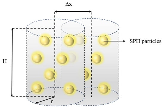
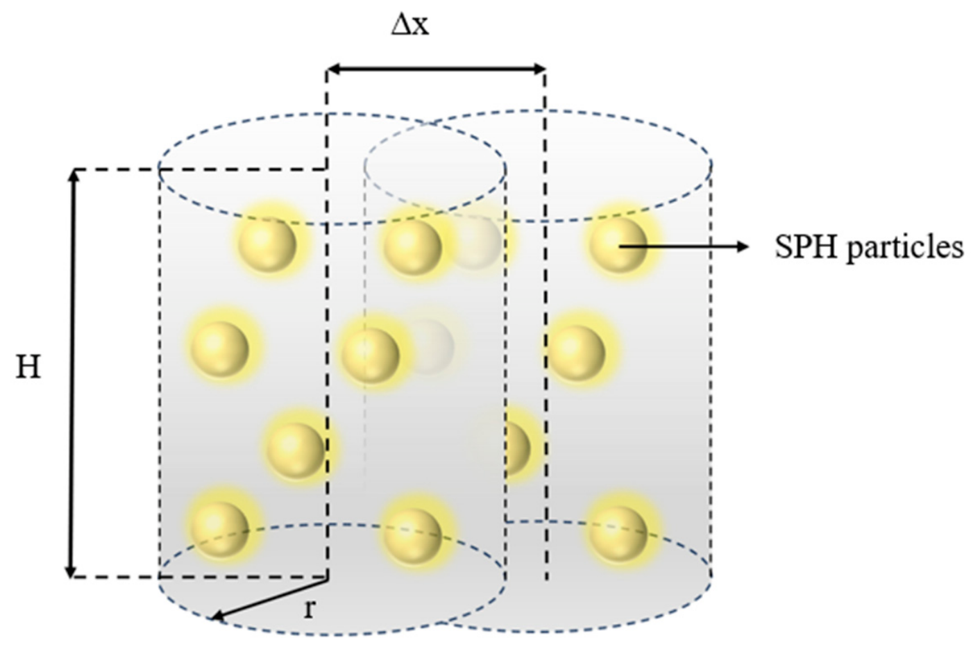
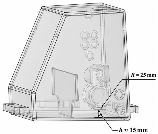
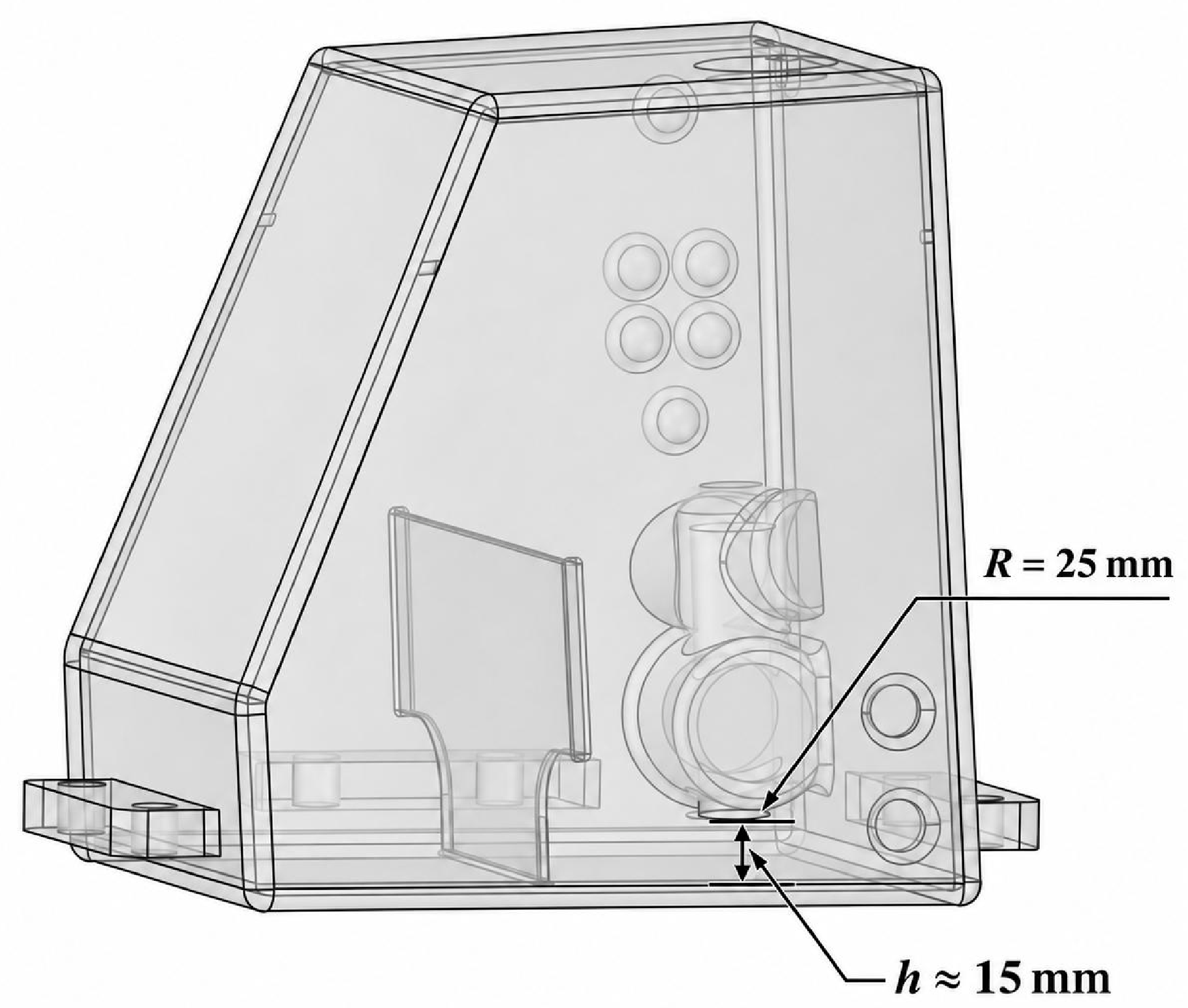
As shown in Figure 2, each virtual sampling domain is represented by a cylindrical region whose axis is perpendicular to the bottom surface of the oil tank. The sampling radius r was set to 25 mm and the sampling height H to 15 mm, based on the actual suction-port geometry and the project-specific design requirements. Specifically, the 25 mm radius corresponds to the radius of the actual suction port, while the 15 mm height is based on the approximate clearance between the suction-port end face and the tank bottom. These dimensions define a local assessment region near the suction port for evaluating lubricant availability. The corresponding project tank and suction-port dimensions are illustrated in Figure 3. The center-to-center spacing between adjacent candidate locations was set to 5 mm, and its influence was examined separately through a spacing-sensitivity analysis.

Figure 2. Schematic illustration of the cylindrical virtual sampling domain and its geometric parameters.

Figure 3. Schematic illustration of the actual tank and the dimensions of the suction port.

Each sampling cylinder is evaluated independently. Adjacent sampling domains may overlap, and the same fluid particle may contribute to the statistics at multiple candidate locations. Because the suction port is installed at the tank bottom and the baffles are perforated, lubricant on both sides of a baffle may contribute to the local lubricant inventory accessible to the inlet through the flow-through openings. Accordingly, when a sampling cylinder intersects a baffle, particles from both sides within the cylinder are included in the local particle-equivalent volume calculation, while the solid volume of the baffle is excluded.

The set of SPH particles located within the i-th virtual sampling domain at time t is denoted as:

$${\mathcal{P}}_{\mathit{i}}\left(\mathit{t}\right)=\{\mathit{p}\mid {\mathit{r}}_{\mathit{p}}(\mathit{t})\in {\mathit{\Omega }}_{\mathit{i}}$$

(1)

where r_p(t) denotes the position of the p-th SPH particle in the tank-fixed coordinate system, and Ω_i denotes the i-th sampling cylinder. Particle inclusion is determined from the particle-center position.

Based on the particle mass and density, the local equivalent lubricant volume at the i-th candidate location at time t is defined as:

$$V_i(t)=\sum _{p\in {\mathcal{P}}_i\left(t\right)}{\displaystyle \frac{m_p}{{\rho }_p\left(t\right)}}$$

(2)

where m_p and ρ_p(t) denote the mass and instantaneous density of the p-th SPH particle, respectively. The equivalent volume of an individual particle is m_p/ρ_p(t), and the sum of the equivalent volumes of all particles within the sampling domain represents the local lubricant volume at that location. This quantity is referred to as the local particle-equivalent lubricant volume. The entire equivalent volume of a particle is included when its center lies within the sampling cylinder.

To use the local pre-maneuver lubricant state at each location as the comparison reference, the mean local particle-equivalent volume during the initial reference period T₀ is taken as the reference value.

The initial reference period was defined as T₀ = [0, 0.5] s, following particle generation and before the prescribed maneuver began. During this interval, the tank remained stationary, and no prescribed translational, rotational, or oscillatory excitation was applied. The mean local particle-equivalent lubricant volume over this interval was used as the reference value for calculating local lubricant availability.

$$V_{i,0}={\displaystyle \frac{1}{N_0}}\sum _{t_k\in T_0}{V}_i\left(t_k\right)$$

(3)

where N₀ denotes the number of time points within the initial reference period.

On this basis, for locations with a positive initial reference volume, the local lubricant availability at the i-th candidate location at time t is defined as:

$$A_i(t)={\displaystyle \frac{V_i\left(t\right)}{V_{i,0}}}\times 100\%$$

(4)

When A_i = 100%, the current local lubricant volume is equal to the initial reference state; when A_i < 100%, the local lubricant volume at that location is reduced relative to the reference state.

Because particle inclusion is determined from the particle-center position and the entire particle-equivalent volume is summed, the crossing of particles at the sampling-cylinder boundary and variations in instantaneous density during maneuvering may cause the instantaneous equivalent volume to exceed the initial reference mean, giving A_i > 100%. Such values indicate an increase in local particle-equivalent lubricant volume relative to the initial reference mean.

2.2. Metrics for Assessing the Local Lubricant State

Based on the local lubricant availability, the local lubricant state at a given location under dynamic operating conditions can be further characterized from three aspects: overall level, extreme state, and persistence.

The overall level is primarily evaluated using the low-percentile local lubricant availability, defined as:

A_5,i = Q₅[A_i(t)]

(5)

where Q₅ denotes the 5th-percentile operator. For computational results saved at equal time intervals, this metric approximately represents the lower bound of local lubricant availability maintained for about 95% of the evaluation period.

Because the low-percentile metric has limited sensitivity to extreme low values occurring at individual time points, the minimum local lubricant availability is further introduced to characterize the most unfavorable local low-oil state within the evaluation period:

$$A_{\min ,i}=\underset{t\in T}{\min }{A}_i(t)$$

(6)

where T denotes the corresponding evaluation period. When A_min,i = 0, the particle-equivalent lubricant volume in the sampling cylinder is zero at least at one computational time point. A_min serves as an auxiliary exclusion criterion in candidate-location screening.

A₅ primarily reflects the low-percentile level of local lubricant availability over the evaluation period. It characterizes the statistical level of low-oil conditions but cannot distinguish whether these conditions are dominated by a single sustained event or comprise multiple short-term fluctuations. The longest continuous low-oil duration L₅₀ is therefore used to describe their temporal characteristics.

Within the evaluation period, each continuous interval during which A_i(t) < 50% is defined as a low-oil event. The longest duration among these events is denoted by L₅₀:

$$L_{50,i}=\underset{e}{\max }(t_{i,e}^{\mathrm{out}}-t_{i,e}^{\mathrm{in}})$$

(7)

where t_in and t_out denote the start and end times of the e-th low-oil event, respectively. The duration L₅₀ is expressed in seconds. If a low-oil event extends across a transition between maneuvering stages, it is treated as one continuous event. If no such event occurs, L₅₀ is set to zero.

2.3. Candidate-Region Screening and Area Assessment

Based on the three evaluation metrics described above, candidate regions are screened over the bottom of the cavity. Candidate locations are required to simultaneously satisfy:

$$A_{5,i}^{\left(\mathrm{s}\right)}\ge 50\%,\mathrm{s}=1,2,3,4;A_{\min ,i}>0;L_{50,i}\le 0.2 \mathrm{s}$$

(8)

where s = 1, 2, 3, and 4 correspond to the dive, pull-up, left-turn, and right-turn-and-recovery stages, respectively. A₅ is evaluated separately for each stage, whereas A_min and L₅₀ are evaluated over the complete maneuvering period. In accordance with the project requirements, the local lubricant state near potential suction-port locations was assessed in terms of extreme depletion, overall availability, and the persistence of low-availability conditions. Since the present study focuses on preliminary suction-port placement rather than the detailed performance of a specific suction port, the thresholds were adopted as reference values for the present assessment.

During lubricant extraction, complete depletion of lubricant near a suction port is undesirable because it may lead to air ingestion and affect continuous lubricant supply. Therefore, A_min was introduced to identify the most unfavorable local lubricant state during the maneuver, and the condition A_min > 0 was used to exclude locations where the particle-equivalent lubricant volume in the sampling cylinder reaches zero.

In addition to avoiding extreme depletion, the project requires attention to the local lubricant state throughout the maneuver. Accordingly, the fifth-percentile availability A₅ was used to characterize the lower level of local lubricant availability in each maneuvering stage. The reference condition A₅ ≥ 50% was adopted to identify locations where a relatively high local lubricant inventory can be maintained during most of each stage.

During continuous maneuvering, attitude changes and inertial effects cause lubricant to redistribute within the tank, and the local availability at a given location may decrease temporarily. The duration of such a reduction is therefore also relevant to the assessment of local lubricant conditions. The longest continuous low-availability duration L₅₀ was introduced to distinguish short-lived reductions from sustained low-availability conditions. A reference limit of L₅₀ ≤ 0.2 s was applied to exclude locations experiencing a prolonged continuous period below 50% availability.

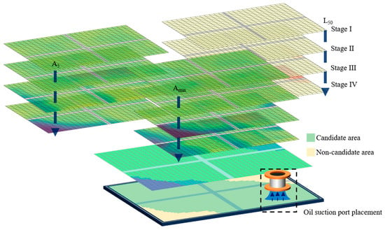
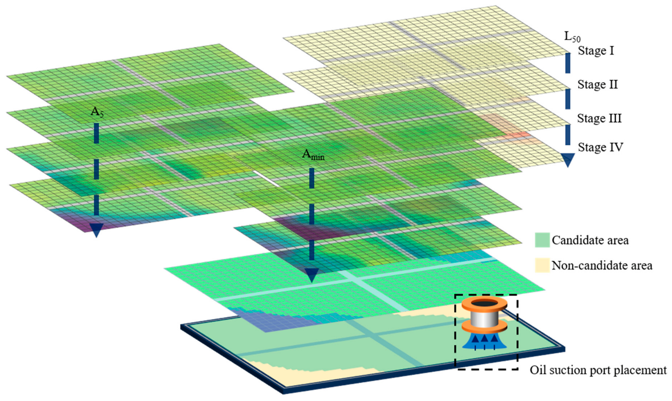
The metrics are calculated from the local lubricant state at each candidate location, and the constraints in Equation (8) are then applied point by point. Locations satisfying all constraints form the candidate region, as illustrated in Figure 4. The region provides a preliminary spatial screening of potential suction port centers and supports subsequent location selection in conjunction with pipeline routing, installation space, and structural constraints.

Figure 4. Schematic illustration of the multi-metric candidate-region screening framework for oil suction port placement.

Considering that different baffle configurations alter the actual evaluable area at the bottom of the cavity, the effective evaluation domain for each configuration is defined as the remaining bottom area after excluding baffles and other regions unsuitable for installation. Its area is denoted by S_valid.

The qualified regions corresponding to the three metrics are spatially intersected to obtain the final candidate region, whose area is denoted by S_candidate. Each 5 mm × 5 mm grid cell in the maps represents one potential suction port location on the tank bottom. The cells satisfying the screening criteria form the candidate region, and its area is calculated by summing their areas.

The candidate-region area ratio is defined as:

$$R_{\mathrm{candidate}}={\displaystyle \frac{S_{\mathrm{candidate}}}{S_{\mathrm{valid}}}}\times 100\%$$

(9)

R_candidate represents the proportion of the effective bottom area, after excluding baffles and other regions unsuitable for installation, that simultaneously satisfies the criteria for local availability, minimum availability, and longest continuous low-oil duration. A larger value indicates a larger retained area of potential suction port centers for the corresponding configuration or operating condition and provides a quantitative comparison among initial oil volumes and baffle configurations.

2.4. SPH Governing Equations and Numerical Method

The built-in divergence-free smoothed particle hydrodynamics (DFSPH) solver in the commercial software Ansys Rocky 2026 R1 is used to simulate lubricant motion in the tank under continuous maneuvering [26,27].

SPH is a mesh-free particle method based on a Lagrangian description. Its fundamental idea is to discretize a continuous fluid into particles carrying physical information such as mass, velocity, density, and pressure, and to solve the fluid motion through interactions among neighboring particles [28,29]. Compared with conventional grid-based computational fluid dynamics methods, SPH does not require a predefined fluid mesh, and fluid interfaces are naturally represented by the spatial distribution of particles. It is therefore well suited for problems involving large free-surface deformation, liquid breakup, and complex moving boundaries [30].

For the lubricant tank considered in this study, pronounced free-surface variations and local liquid separation occur during lubricant motion. Conventional grid-based methods require additional treatment of mesh deformation and interface capturing, whereas SPH directly tracks the motion of fluid particles and can therefore provide the time-dependent lubricant distribution at different spatial locations. Accordingly, SPH is employed to simulate lubricant migration inside the tank during maneuvering, and the resulting particle information is further used to evaluate the local lubricant state.

Under the Lagrangian formulation, fluid motion satisfies the mass- and momentum-conservation equations [31]:

$${\displaystyle \frac{\mathrm{D}\rho }{\mathrm{D}t}}=-\rho \nabla ·\mathbf{v}$$

(10)

$${\displaystyle \frac{\mathrm{D}\mathbf{v}}{\mathrm{D}t}}=-{\displaystyle \frac{1}{\rho }}\nabla p+{\displaystyle \frac{1}{\rho }}\nabla ·\mathit{\tau }+\mathbf{g}$$

(11)

where ρ denotes the fluid density, v the velocity vector, p the pressure, τ the viscous stress tensor, and g the external acceleration term.

In the SPH method, continuous field variables are discretized through kernel functions. The approximation of an arbitrary physical quantity f at particle i can be expressed as:

$$f_i=\sum _j{\displaystyle \frac{m_j}{{\rho }_j}}{f}_{j}W({\mathit{r}}_i-{\mathit{r}}_j,h)$$

(12)

where m_j, ρ_j, and f_j denote the mass, density, and corresponding physical quantity of neighboring particle j, respectively; r_i and r_j denote the particle positions; W is the kernel function; and h is the smoothing length. The kernel function limits particle interactions to a finite neighborhood, thereby transforming the continuous field variable into a discrete form based on summation over neighboring particles.

Applying the above kernel approximation to the governing equations, the mass-conservation equation can be further written in particle form as:

$${\displaystyle \frac{\mathrm{d}{\rho }_i}{\mathrm{d}t}}=\sum _j{m}_j({\mathbf{v}}_i-{\mathbf{v}}_j)·{\nabla }_i{W}_{\mathit{ij}}$$

(13)

Correspondingly, the momentum equation can be expressed in discrete form by accounting for interparticle pressure forces, viscous forces, and external acceleration:

$${\displaystyle \frac{\mathrm{d}{\mathbf{v}}_i}{\mathrm{d}t}}=-\sum _j{m}_j({\displaystyle \frac{p_i}{{\rho }_i^2}}+{\displaystyle \frac{p_j}{{\rho }_j^2}}){\nabla }_i{W}_{\mathit{ij}}+{\mathbf{F}}_i^{\mathrm{vis}}+\mathbf{g}$$

(14)

where v_i denotes the velocities of particle i; m_j, p_i, p_j, ρ_i and ρ_j denote the mass, pressure, and density of the corresponding particles, respectively; W_ij is the kernel function; ∇_i W_ij denotes its gradient with respect to the position of particle i, and ${\mathbf{F}}_i^{\mathrm{vis}}$ denotes the viscous force per unit mass acting on particle i. Through this particle discretization, the velocity, position, and related physical states are updated over time, while the motion and evolution of the free surface are represented by the spatial distribution of the particles.

DFSPH constrains density deviations through the pressure solution and imposes a divergence-free constraint on the velocity field to satisfy the requirements of incompressible flow [26,27]. Viscous effects are represented using the Cleary discretization [32], and turbulence is represented using the built-in large eddy simulation (LES) model. The molecular and turbulent viscosities together constitute the effective viscosity used in the viscous calculation [27].

Through this discretized formulation, SPH converts the fluid governing equations into local interaction calculations among particles and describes the migration and spatial redistribution of the lubricant free surface through the temporal evolution of particle states. The resulting time-series information of particle positions and physical states provides the data basis for subsequent extraction of local lubricant distributions and assessment of the local lubricant state.

2.5. Numerical Model Validation

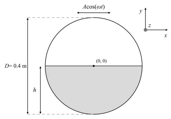
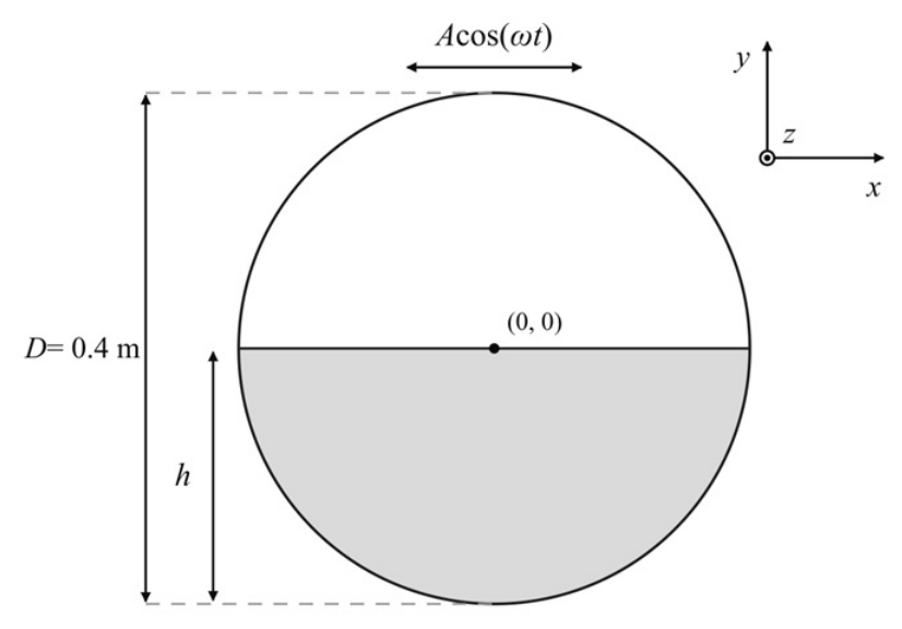
As shown in Figure 5, to assess the prediction of forced free-surface motion by the adopted SPH method, validation is performed using the experimental data published by Brown et al. (2025) for CCP-WSI Test Case 17, formerly CCP-WSI Blind Test Series 5 [33], together with the circular-tank sloshing comparison reported by Brown et al. (2026) in Ocean Engineering [34]. The horizontal-excitation case 2HIBT5, designated H1 in the comparative study [34], is selected. Free-surface displacement histories on the left and right sides of the tank are compared with the experiments, and the root-mean-square error (RMSE) is calculated. This comparison assesses the predicted free-surface response and supports the subsequent simulation of lubricant migration and spatial distribution under continuous maneuvering.

Figure 5. Benchmark tank schematic reproduced from the CCP-WSI Test Case 17 webpage; the experimental dataset and comparative study are described in [33,34]. Coordinates and the illustrative liquid level follow the original source. The present H1 model and its nominal initial water depth of 120 mm are shown in Figure 6.

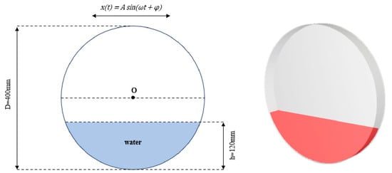
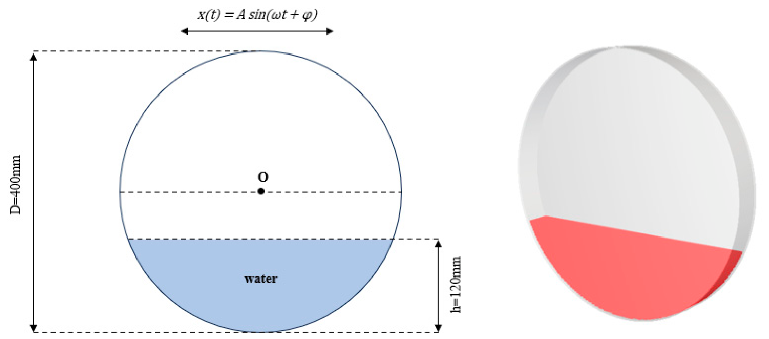
The experimental tank is a horizontal cylinder with an internal diameter of 400 mm, an internal axial width of 40 mm, and a nominal initial water depth of 120 mm measured upward from the lowest point of the inner wall. The origin is placed at the center of the circular cross-section, with Y along the cylinder axis, X in the horizontal excitation direction, and Z vertically upward. The nominal still-water surface is therefore at Z = −80 mm. A horizontal harmonic translation with an amplitude of 2 mm and a frequency of 1.3 Hz is imposed along X, with the initial motion in the negative X direction. The numerical simulation includes an initial 4 s stationary period followed by 20 s of horizontal excitation, giving a total duration of 24 s. Taking the onset of excitation as the comparison time origin, τ = t − 4 s, where t is the simulation time, the horizontal tank displacement relative to its initial position is:

$$q_x(t)=\left\{\begin{array}{cc}0,& 0\le t<4 \mathrm{s}\\ a\left[\cos \right(2\mathit{\pi f\tau })-1],& 4\le t\le 24 \mathrm{s}\end{array}\right.$$

(15)

where a = 2 mm and f = 1.3 Hz. The two-dimensional dimensions and three-dimensional geometry of the present H1 validation model are shown in Figure 6.

Figure 6. Present H1 horizontal-sloshing validation model. (Left): two-dimensional dimensions and horizontal harmonic excitation, with an internal diameter D = 400 mm and nominal initial water depth h = 120 mm. (Right): three-dimensional tank and initial fluid domain. The horizontal displacement amplitude is 2 mm and the excitation frequency is 1.3 Hz.

The DFSPH solver is used, with water treated as a constant-property fluid of density 998 kg/m³ and dynamic viscosity 0.001002 Pa·s. The initial particle spacing is 2 mm. The Wendland kernel is used with a kernel-scale factor of 1.25, together with the Cleary viscosity discretization, LES turbulence model, and a no-slip turbulent wall boundary. The principal numerical parameters are listed in Table 1.

Table 1. Principal numerical parameters of the circular-tank sloshing validation case.

Parameter	Value or Setting
SPH solver	DFSPH
Initial particle spacing	2 mm
Kernel function	Wendland
Kernel-scale factor	1.25
Fluid density	998 kg/m3
Dynamic viscosity	0.001002 Pa·s
Gravitational acceleration	9.81 m/s2, along −Z
Viscosity model	Cleary
Turbulence model	LES, CS = 0.2
Wall boundary	No Slip Turbulent
SPH time-step factor	0.25
Initial stationary period	4 s
Excitation duration	20 s

During post-processing, particle positions are first transformed into the tank-fixed coordinate system. Free-surface sampling paths are defined at the mid-plane Y = 0, horizontally offset by 2.3 mm into the water from the left and right curved walls. A local liquid-indicator field is reconstructed using a particle-volume-weighted Wendland kernel with a reconstruction scale of 2.5 mm, and the interface is identified at an indicator value of 0.5. Each sampling path is searched upward to locate the free surface connected to the bottom liquid, and its height is obtained by linear interpolation between adjacent sampling points. The free-surface displacement η is defined relative to the nominal still-water level Z = −80 mm. Simulation results at 4–24 s are aligned with experimental data at 0–20 s after excitation onset, and the numerical histories are interpolated to the experimental sampling times for comparison.

The RMSE between the numerical and experimental free-surface displacement histories is calculated as:

$${\mathrm{RMSE}}_{\eta }=\sqrt{{\displaystyle \frac{1}{N_{\eta }}}{\displaystyle \sum _{j=1}^{N_{\eta }}}{\left[{\eta }_{\mathrm{sim}}\right({\tau }_j)-{\eta }_{\exp }({\tau }_j\left)\right]}^2}$$

(16)

where N_η is the number of comparison times, and η_sim and η_exp are the numerical and experimental free-surface displacements, respectively. RMSE is expressed in millimeters and quantifies the overall difference between the numerical predictions and experimental measurements over the comparison period.

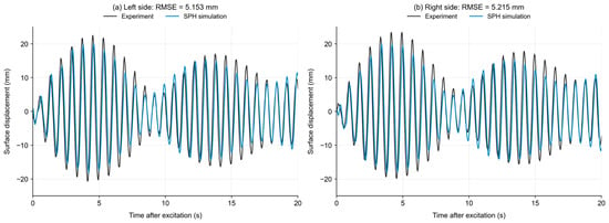
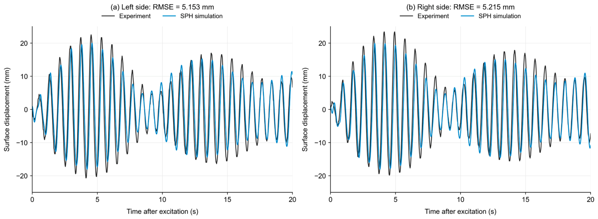
Figure 7 compares the numerical and experimental free-surface displacement histories on the left and right sides. The numerical results reproduce the periodic oscillation and the sequence of increasing, decreasing, and increasing amplitudes observed in the experiments. The principal trends on both sides are consistent with the measurements. Over the first 20 s after excitation onset, the RMSE values are 5.153 mm on the left and 5.215 mm on the right. The temporal response and error measures indicate that the model reasonably describes the free-surface dynamics under the investigated condition.

Figure 7. Numerical and experimental free-surface displacement histories under horizontal sloshing: (a) left side; (b) right side. Time is measured from the onset of excitation.

Overall mass conservation is also checked using the fluid-particle count and total mass at all 2401 saved time points over 0–24 s. The particle count remains 158,535 and the total mass remains approximately 1.265744 kg, with no changes in either quantity observed in the saved results.

The free-surface comparisons, RMSE values, and mass statistics indicate that the adopted SPH method captures the principal free-surface motion under the investigated horizontal-sloshing condition, providing a basis for the subsequent numerical study of lubricant free-surface motion and spatial distribution under continuous maneuvering.

2.6. Sensitivity to Numerical Resolution and Screening Parameters

The effects of spatial sampling, temporal sampling, screening conditions, and particle discretization are examined through analyses of sampling-center spacing, result-saving interval, screening thresholds, and particle resolution, respectively. Post-processing and screening parameters are first examined using the results obtained with a 5 mm particle spacing. Candidate regions obtained with different particle spacings are then compared under consistent assessment conditions.

The sampling-center-spacing, result-saving-interval, and particle-resolution analyses use the 10 L cross-baffle case. The threshold analysis considers the no-baffle, XY-baffle, YZ-baffle, and cross-baffle configurations at the same initial oil volume. The sampling-cylinder radius and height are fixed at 25 mm and 15 mm, respectively. The mean particle-equivalent volume at each location over 0–0.5 s is used as the reference, and the evaluation period is 0.5–7.2 s. The baseline criteria are stage-wise A₅ ≥ 50%, complete-period A_min > 0, and L₅₀ ≤ 0.2 s. Only the parameter under investigation is varied in each analysis.

Changes in the screening results are evaluated using the candidate-region area ratio and intersection over union (IoU). The area ratio is calculated from the bottom area represented by the retained locations relative to the effective bottom area. Results for different parameters within the same configuration are mapped to a common effective bottom domain, and IoU is defined as:

$$\mathrm{IoU}={\displaystyle \frac{|{\mathit{\Omega }}_{\mathrm{test}}\cap {\mathit{\Omega }}_{\mathrm{ref}}|}{|{\mathit{\Omega }}_{\mathrm{test}}\cup {\mathit{\Omega }}_{\mathrm{ref}}|}}\times 100\%$$

(17)

where Ω_test and Ω_ref denote the candidate regions of the evaluated and reference results, respectively, and |·| denotes area. A higher IoU indicates closer spatial overlap between the two candidate regions. Threshold comparisons among the four configurations use the effective bottom area of each configuration to calculate the area ratio and compare their ranking.

2.6.1. Effect of Sampling-Center Spacing

The sampling-center spacing determines the density of candidate locations over the tank bottom. Spacings of 2.5 mm, 5 mm, and 10 mm are examined while keeping the particle spacing at 5 mm, the saving interval at 0.05 s, and the sampling-cylinder dimensions unchanged. Local availability and screening metrics are calculated independently for each arrangement. The retained locations are mapped to the same effective bottom domain using their represented areas, with the 2.5 mm result used as the reference.

As shown in Table 2, the candidate-region area ratios range from 59.235% to 59.515%, with differences of no more than 0.280 percentage points relative to the 2.5 mm reference. The IoU values for 5 and 10 mm are 98.06% and 96.33%, respectively, indicating that the area and spatial distribution of the candidate region are relatively insensitive to sampling-center spacing within the investigated range. The area ratio for 5 mm differs from that for 2.5 mm by only 0.159 percentage points, with close spatial agreement. A smaller spacing provides finer candidate-location resolution but increases the number of sampling locations and the post-processing workload. A center spacing of 5 mm is therefore adopted to balance spatial detail and computational effort.

Table 2. Candidate-region comparison for different sampling-center spacings.

Sampling-Center Spacing/mm	Candidate-Region Area Ratio/%	Difference from 2.5 mm/pp	IoU Relative to 2.5 mm/%
2.5	59.235	0.000	100.00
5	59.394	0.159	98.06
10	59.515	0.280	96.33

2.6.2. Effect of Result-Saving Interval

With the sampling-center spacing fixed at 5 mm, temporal sampling is examined for its effects on local low-oil identification and candidate regions. Time series with intervals of 0.10 s and 0.20 s are subsampled from the original 0.05 s results. The initial reference volume at each location is held fixed, and A₅, A_min, L₅₀, and their joint screening result are recalculated. Sampling starts at 0.5 s, and the evaluation endpoint at 7.2 s is retained. The 0.05 s result is used as the reference. The comparison results for different result-saving intervals are summarized in Table 3.

Table 3. Candidate-region comparison for different result-saving intervals.

Result-Saving Interval/s	Candidate-Region Area Ratio/%	Difference from 0.05 s/pp	IoU Relative to 0.05 s/%
0.05	59.394	0.000	100.00
0.10	61.394	2.000	95.87
0.20	65.091	5.697	90.98

Increasing the saving interval from 0.05 s to 0.10 s and 0.20 s increases the candidate-region area ratio by 2.000 and 5.697 percentage points, with IoU values of 95.87% and 90.98%, respectively. Temporal sampling therefore affects the identification of local low-oil conditions and, consequently, the jointly screened region. Compared with the coarser series, the 0.05 s results retain more detailed information on liquid migration and short low-oil events. A saving interval of 0.05 s is therefore used for subsequent metric calculation and candidate-region screening.

2.6.3. Effect of Screening Thresholds

After fixing the spatial and temporal sampling conditions, the effects of varying assessment requirements on the candidate regions and configuration comparisons are examined. The baseline conditions are A₅ ≥ 50%, A_min > 0, and L₅₀ ≤ 0.2 s. The lower bound of A₅ and upper bound of L₅₀ are varied. For the four configurations at 10 L and a particle spacing of 5 mm, A_min > 0 is held fixed. The A₅ lower bound is first set to 40%, 50%, and 60%, with the L₅₀ upper bound fixed at 0.2 s. The A₅ lower bound is then fixed at 50%, and the L₅₀ upper bound is set to 0.1 s, 0.2 s, and 0.4 s. Throughout these comparisons, a low-oil event for L₅₀ remains defined by local availability below 50%.

As shown in Table 4, raising the A₅ lower bound or reducing the L₅₀ upper bound decreases the candidate-region area. For all threshold combinations tested, the ranking by candidate-region area ratio remains cross baffle, YZ baffle, XY baffle, and no baffle. The configuration comparison is therefore consistent over the investigated range of assessment requirements. These reference thresholds provide a common basis for comparing the local lubricant state and candidate regions among configurations.

Table 4. Candidate-region area ratios of the four configurations under different screening thresholds.

A5 Lower Bound/%	L50 Upper Bound/s	No Baffle/%	XY Baffle/%	YZ Baffle/%	Cross Baffle/%
40	0.2	10.24	22.06	50.76	63.39
50	0.2	4.19	17.29	45.13	59.39
60	0.2	0.71	11.94	38.81	54.94
50	0.1	1.33	8.32	36.42	52.12
50	0.4	4.19	17.29	45.13	59.39

2.6.4. Effect of Particle Resolution

Under the sampling and baseline screening conditions established above, initial particle spacings of 4 mm, 5 mm, 6 mm, and 7 mm are considered for the 10 L cross-baffle case. The tank structure, target initial oil volume, fluid properties, prescribed motion, and remaining numerical settings are held constant. The sampling-center spacing is 5 mm and the saving interval is 0.05 s. The 4 mm result is used as the reference.

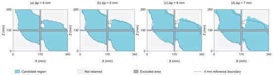
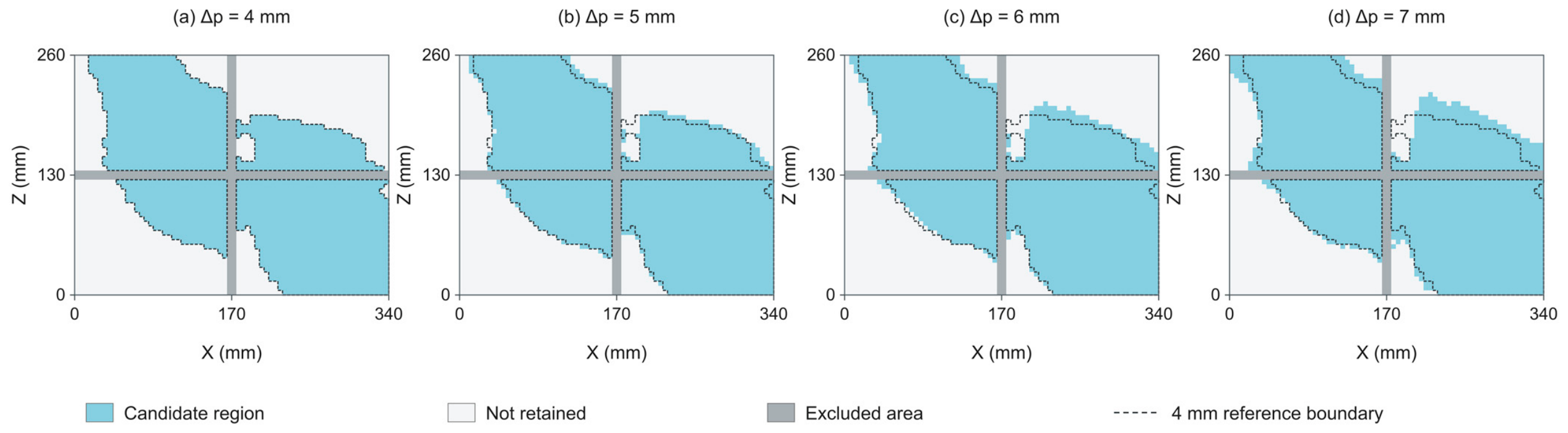
Figure 8 shows that the principal candidate-region locations are generally consistent among particle spacings. With particle refinement, the area and boundary approach the 4 mm reference result. Table 5 summarizes the candidate-region area ratios and IoU values.

Figure 8. Candidate regions obtained with different particle spacings for the 10 L cross-baffle case: (a) 4 mm; (b) 5 mm; (c) 6 mm; (d) 7 mm. Blue denotes the candidate region satisfying the joint criteria, light gray denotes the other locations in the effective bottom domain, and dark gray denotes excluded locations. The black dashed line marks the boundary of the 4 mm reference candidate region.

Table 5. Candidate-region comparison for different particle spacings.

Particle Spacing/mm	Candidate-Region Area Ratio/%	IoU Relative to 4 mm/%
4	57.39	100.00
5	59.39	95.34
6	60.30	92.66
7	62.88	89.45

As the particle spacing decreases from 7 mm to 6 mm and 5 mm, IoU relative to the 4 mm reference increases from 89.45% to 92.66% and 95.34%, respectively, indicating increasing spatial agreement with refinement. The area ratios for 5 mm and 4 mm are 59.39% and 57.39%, respectively, a difference of 2.00 percentage points, and the two regions exhibit close spatial overlap. The initial fluid-particle count for 5 mm is approximately 51.2% of that for 4 mm. Considering both screening consistency and computational scale, a particle spacing of 5 mm is adopted for the subsequent tank simulations.

2.7. Oil-Tank Model and Baffle Configurations

Baffles regulate lubricant motion within the tank, while their arrangement and geometry also affect the available space for suction port placement and local lubricant redistribution during maneuvering. Different baffle configurations are therefore considered to compare their effects on the local lubricant state and candidate-region distribution.

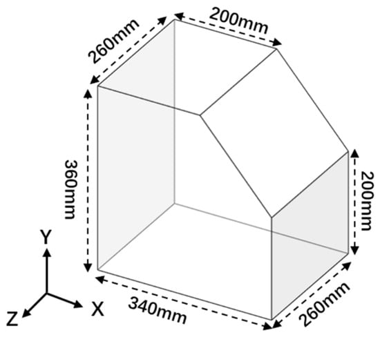
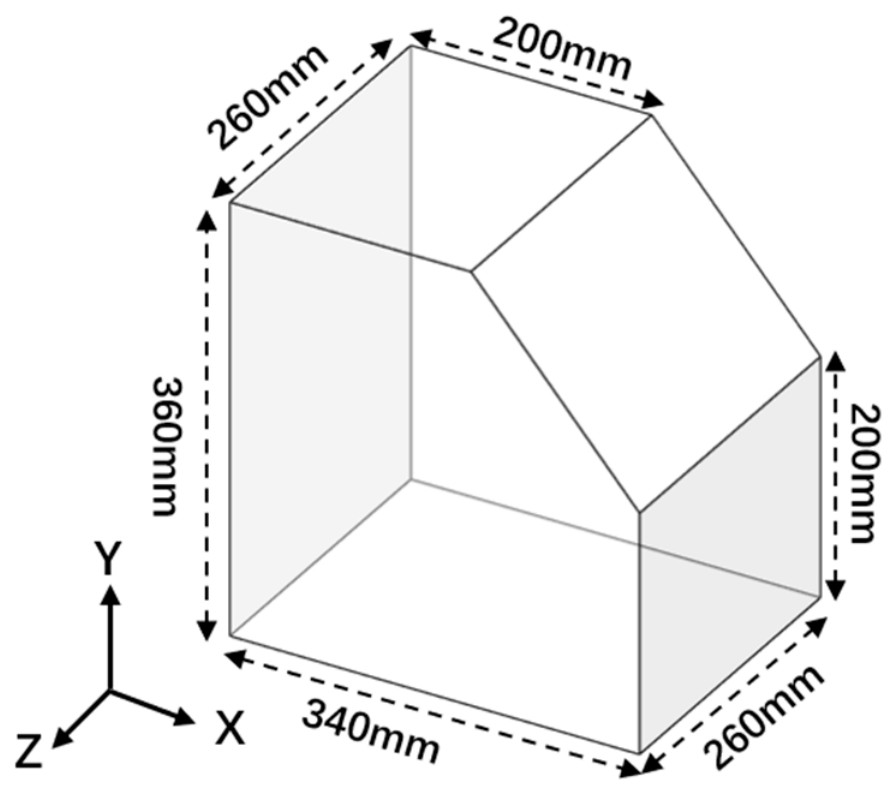
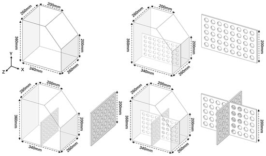
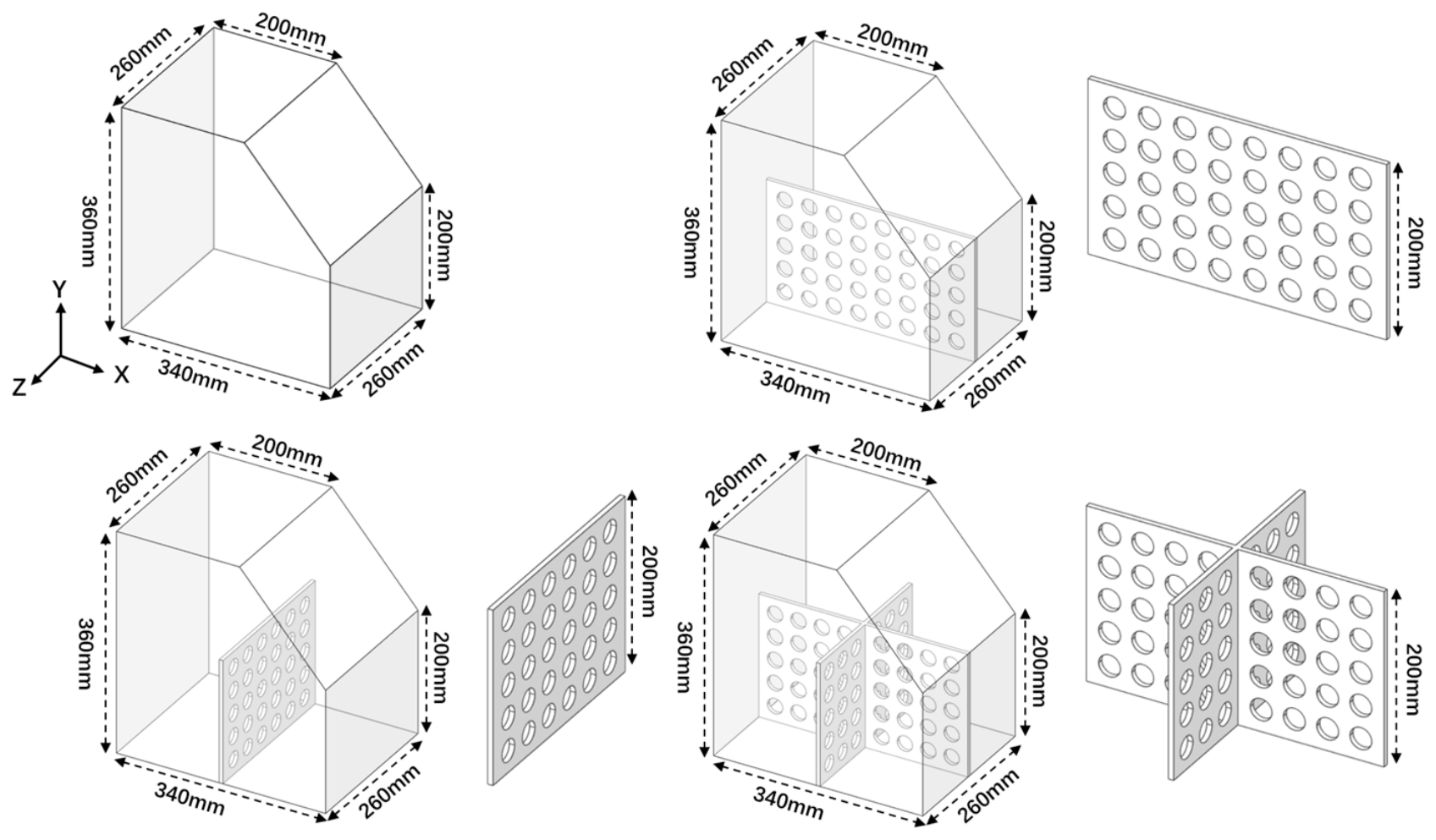
The lubricant tank model used in this study is shown in Figure 9, with bottom dimensions of 340 mm × 260 mm. While keeping the main tank geometry unchanged, four configurations are considered: no baffle, an XY-plane baffle (longitudinal baffle), a YZ-plane baffle (transverse baffle), and a cross baffle, to compare the effects of baffle arrangement on lubricant distribution.

Figure 9. Lubricant tank model and main dimensions.

All baffles are perforated, with a height of 200 mm, a thickness of 6 mm, circular flow-through holes of 25 mm in diameter, and an open-area ratio of 30%. The XY baffle is 340 mm in length, while the YZ baffle is 260 mm in length. The cross baffle is formed by combining the two. The four configurations are shown in Figure 10.

Figure 10. Schematic illustration of the four baffle configurations.

2.8. Numerical Parameters and Maneuvering Conditions

To investigate the effect of initial oil volume on the local lubricant state, three initial volumes of 10 L, 13 L, and 16 L are considered, representing low, medium, and high oil-volume conditions, respectively. Each group includes the no-baffle, XY-baffle, YZ-baffle, and cross-baffle configurations, resulting in 12 cases. Except for the initial oil volume and baffle configuration, the maneuvering conditions, fluid model, and numerical settings are identical.

AeroShell Turbine Oil 555 was selected as the reference lubricant and modeled as a constant-property Newtonian fluid. The reference density was set to 993 kg/m³ at 15.6 °C, and the reference kinematic viscosity was 26.5 mm²/s at 40 °C, as reported in the manufacturer’s Technical Data Sheet [35]. Using the relationship μ = ρν and considering the small density change between those two temperatures, the dynamic viscosity at 40 °C used in the simulations was 0.0263 Pa·s, which is treated as a nominal simulation input.

The principal numerical parameters are listed in Table 6.

Table 6. Numerical parameters of the main simulation cases.

Parameter	Setting
Software	Ansys Rocky 2026 R1
SPH solver	DFSPH
Initial oil volume	10 L, 13 L, 16 L
Reference density	993 kg/m3
Reference dynamic viscosity	0.0263 Pa·s
Initial particle spacing	5 mm
Kernel and scale factor	Wendland; 1.25
Viscosity discretization	Cleary
Turbulence model	LES
Wall boundary	No Slip Turbulent
Time-step factor	0.25
Result-saving interval	0.05 s
Total simulation duration	8 s
Gravitational acceleration	9.81 m/s2

The tank walls and internal baffles are treated as rigid boundaries, with the No Slip Turbulent boundary condition applied between the fluid and walls.

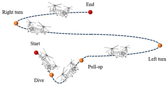
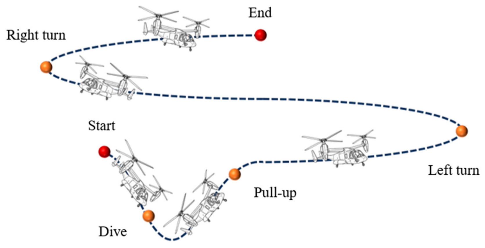
To characterize transient lubricant migration under continuous maneuvering, a prescribed sequence of dive, pull-up, left-turn, and right-turn-and-recovery motions is applied, as shown in Figure 11. The tank is initially stationary over 0–0.5 s, and the principal maneuvering period is 0.5–7.2 s. The tank and baffles follow the same prescribed rigid-body motion, and the virtual sampling domains are fixed in the tank-fixed coordinate system and move synchronously with the tank.

Figure 11. Schematic of the continuous maneuvering trajectory.

The origin is placed at a corner of the initial tank bottom, with X along the 340 mm edge, Y vertically upward, and Z along the 260 mm edge. Gravity acts in the −Y direction. The initial cavity center is used as the maneuver reference point. Pitch, roll, and turn motions are defined about the Z, X, and Y axes of their respective local motion frames and combined through nested coordinate systems. Positive rotation follows the right-hand rule.

The left-turn center is offset by 2 m along the local −Z direction from the left-roll reference point, which coincides with the initial cavity center. The right-roll reference point is offset by 2 m along the local +Z direction from the left-turn center, and the right-turn center is offset by another 2 m along the local +Z direction from the right-roll reference point. Each offset is defined in its parent motion frame; the turn centers and rotation axes therefore move with the preceding motions.

The parameters of the individual motion components are listed in Table 7. The axes are local to the corresponding motion frames, and the signs of velocity and acceleration are defined relative to those local axes.

Table 7. Parameters of the individual motion components in the continuous maneuver.

Time/s	Motion Component	Local Axis	Initial Velocity/Angular Velocity	Acceleration/Angular Acceleration
0.5–1.3	Dive rotation	Z	−15 °/s	0
0.5–1.3	Accelerating translation	X	0 m/s	+1.5 m/s2
1.3–2.1	Pull-up rotation	Z	+15 °/s	0
1.3–2.1	Decelerating translation	X	+1.2 m/s	−1.5 m/s2
2.1–2.6	Initial roll	X	−60 °/s	0
2.1–2.6	Left-turn acceleration	Y	0 °/s	+200 °/s2
2.6–3.9	Constant-speed left turn	Y	+100 °/s	0
3.9–4.4	Left-turn deceleration	Y	+100 °/s	−200 °/s2
3.9–4.9	Roll attitude transition	X	−60 °/s	0
4.4–4.9	Right-turn acceleration	Y	0 °/s	−200 °/s2
4.9–6.2	Constant-speed right turn	Y	−100 °/s	0
6.2–6.7	Right-turn deceleration	Y	−100 °/s	+200 °/s2
6.2–6.7	Recovery acceleration	X	0 °/s	−120 °/s2
6.7–7.2	Recovery deceleration	X	−60 °/s	+120 °/s2

The angular-displacement magnitudes of the dive and pull-up are both 12°, and the accumulated local turning angles are 180° for both the left and right turns.

The initial roll over 2.1–2.6 s is applied about the local X axis of the left-roll frame. The attitude transition over 3.9–4.9 s is applied about the local X axis of the right-roll frame, which changes orientation with the preceding left-turn motion. After the accumulated 180° left turn, this latter local X axis points opposite to the initial X direction.

The roll transition starts at 3.9 s and spans the left-turn deceleration and right-turn acceleration stages. Attitude recovery starts at 6.2 s and overlaps the right-turn deceleration. The recovery-acceleration and recovery-deceleration frames are nested sequentially after the right-turn-deceleration frame. The two recovery components act about their respective local X axes, which have the same direction. Under the combined motion, the tank is inclined by approximately 30° toward opposite sides at 2.6 s and 4.9 s and returns to its initial attitude at 7.2 s.

Over 7.2–8.0 s, the tank remains at its end-of-maneuver position and initial attitude while lubricant flow continues to be calculated. This interval is excluded from the local lubricant availability assessment, whose evaluation period is 0.5–7.2 s.

3. Results and Discussion

3.1. Overall Effects of Initial Oil Volume and Baffle Configuration on Candidate Regions

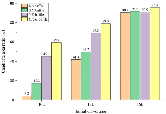
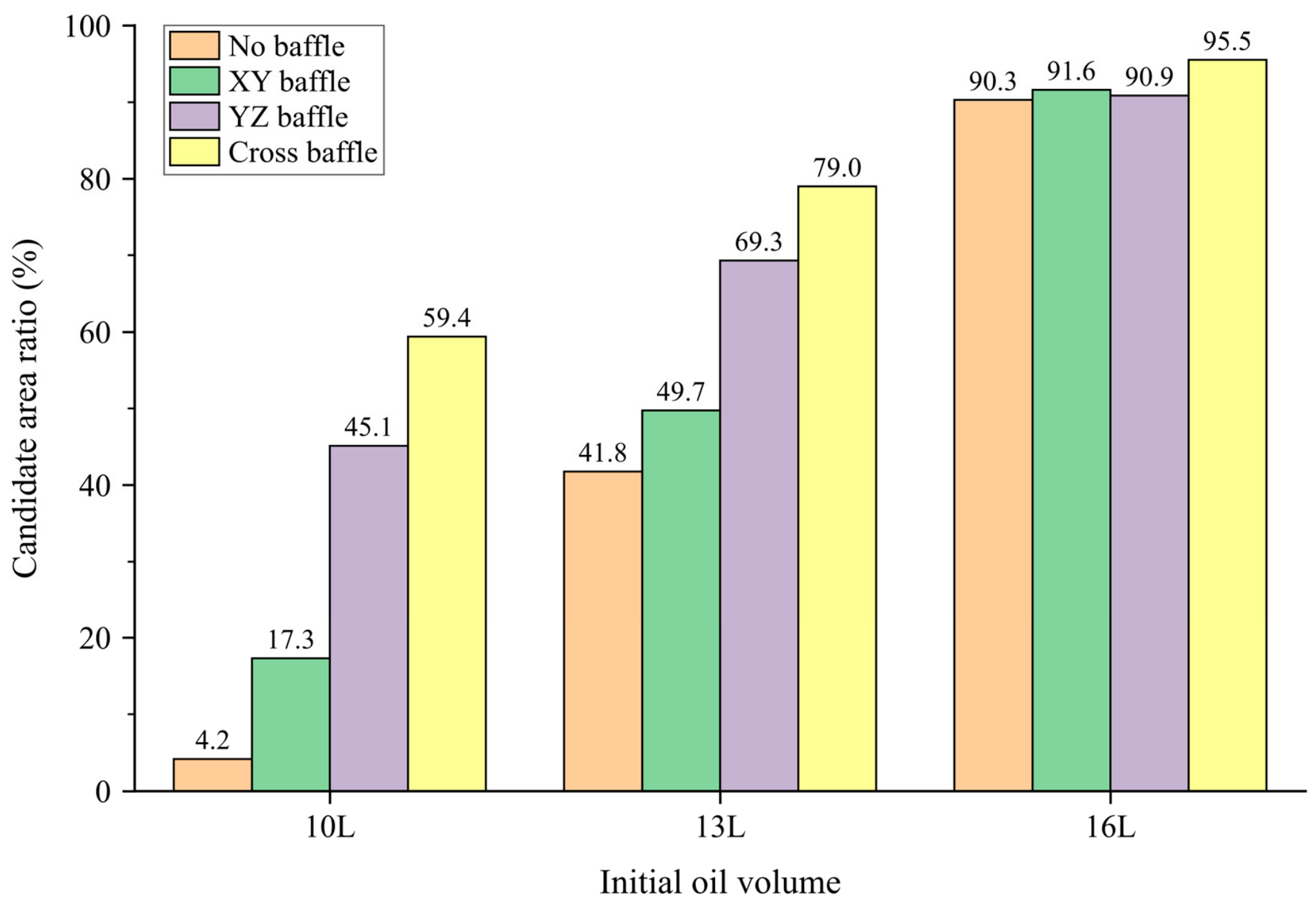
Figure 12 presents the candidate-region area ratios for the different initial oil volumes and baffle configurations. The denominator is the effective bottom area of each configuration after excluding baffles and other regions unsuitable for installation. Overall, the candidate-region area ratio increases for all configurations as the initial oil volume increases from 10 L to 13 L and 16 L. The ratios range from 4.19% to 59.39% for 10 L, from 41.77% to 79.00% for 13 L, and from 90.27% to 95.52% for 16 L.

Figure 12. Candidate-region area ratios for different initial oil volumes and baffle configurations.

Differences among baffle configurations become more pronounced as the oil volume decreases. For 10 L, the area ratios are 4.19%, 17.29%, 45.13%, and 59.39% for the no-baffle, XY-baffle, YZ-baffle, and cross-baffle configurations, respectively. At a lower oil volume, maneuver-induced lubricant migration more readily produces low-oil conditions at some bottom locations, making the candidate region more sensitive to baffle arrangement. By constraining migration between compartments, the baffles alter local lubricant retention; at lower volumes, these changes more readily determine whether a location satisfies the screening criteria.

The cross-baffle configuration provides the largest candidate-region area ratio in all three volume groups. The results for the different configurations are relatively close at 16 L. With more lubricant, a larger part of the bottom can retain local conditions satisfying the assessment requirements during migration, and the candidate-region area ratios become more similar.

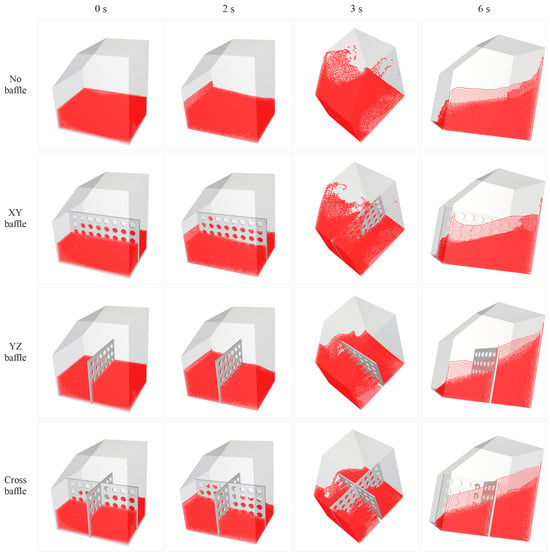
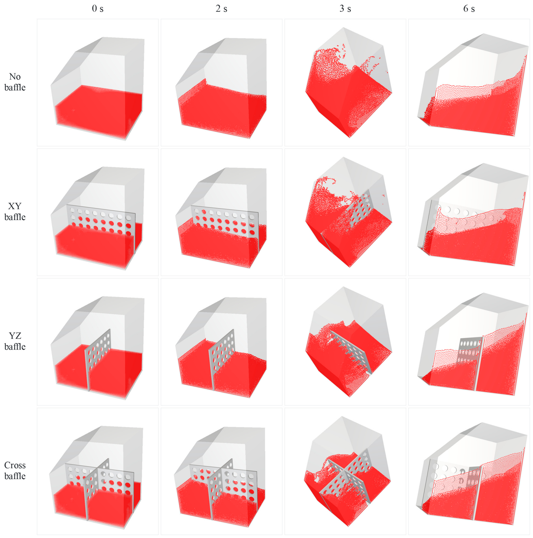
Figure 13 shows the transient lubricant distributions of the four baffle configurations at selected times.

Figure 13. Transient lubricant distributions under four baffle configurations at 0, 2 s, 3 s, and 6 s.

3.2. Local Lubricant State Under the Low-Volume Condition

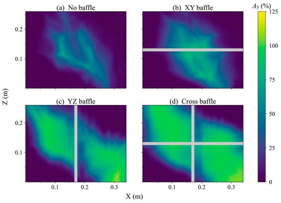
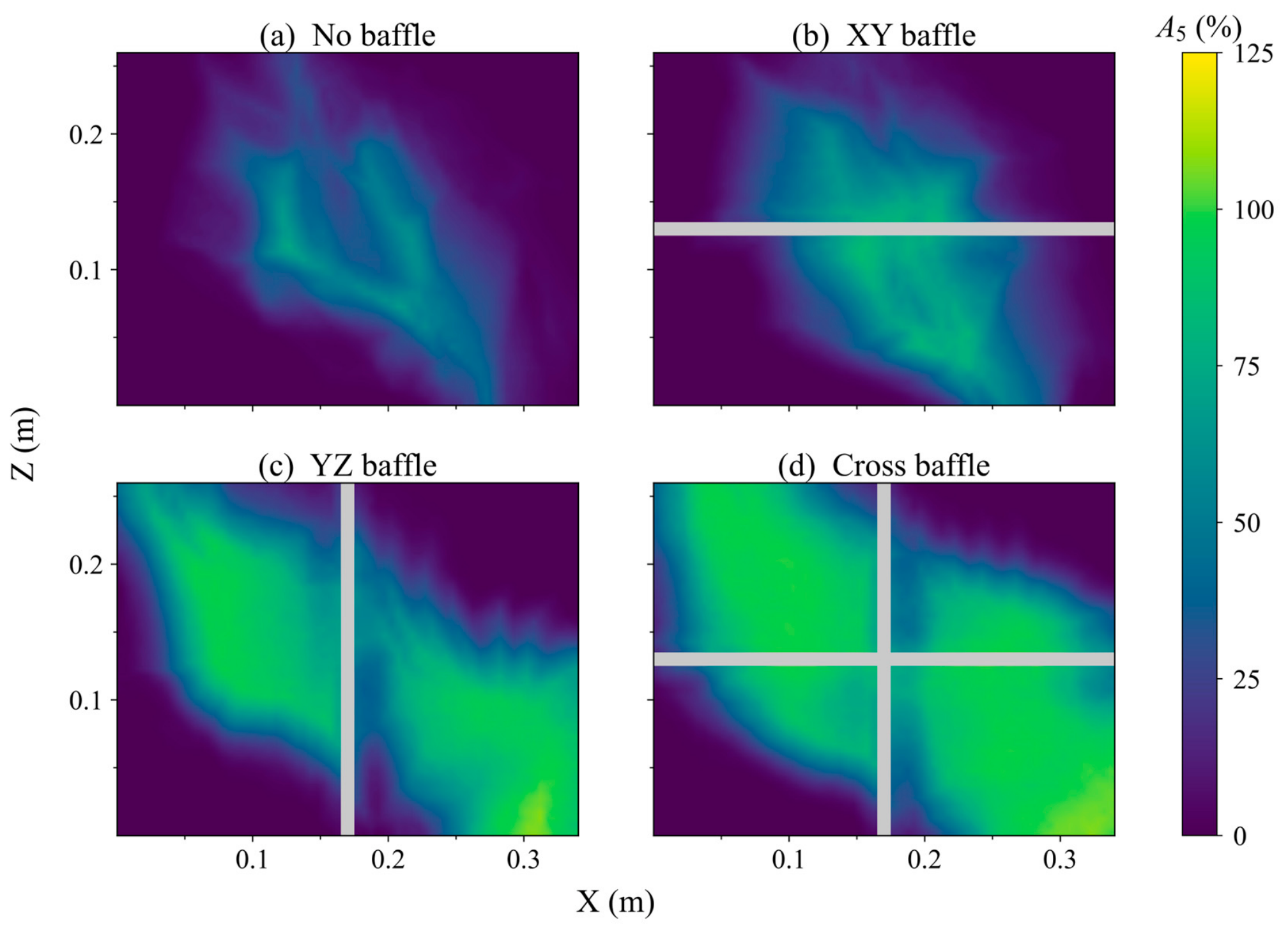
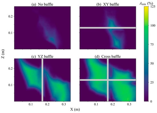
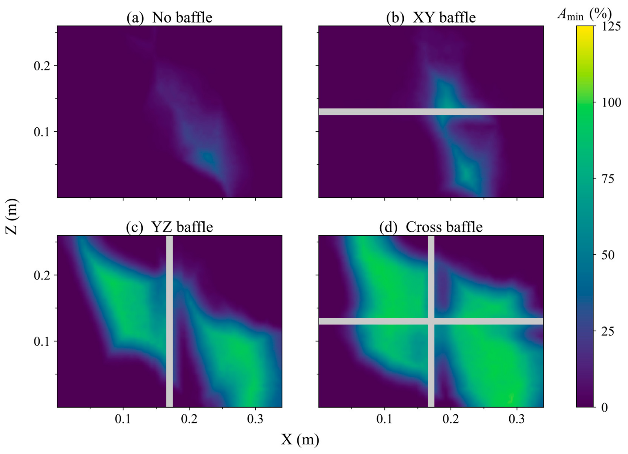
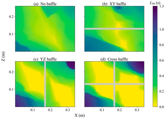
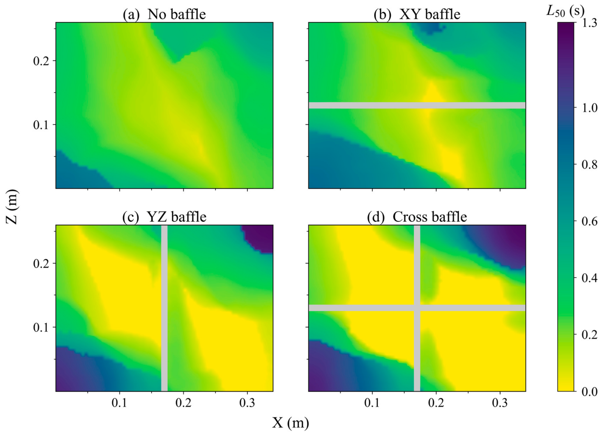
Because the candidate regions are smallest at 10 L and the differences among baffle configurations are relatively pronounced, this group is selected for further analysis of the local lubricant state. In practical aviation operation, lubricant quantity may decrease under emergency or weight-reduction conditions while the normal lubrication of critical components must still be maintained. A lower initial oil volume therefore provides a representative condition for examining local lubricant deficiency and the effects of baffle configuration. Figure 14, Figure 15 and Figure 16 show the spatial distributions of A₅, A_min, and L₅₀ used for screening. A₅ is the minimum of the four stage-wise values, whereas A_min and L₅₀ are evaluated over the complete maneuvering period.

Figure 14. Spatial distributions of screening A₅ for the four configurations at 10 L. Each location uses the minimum of its four stage-wise A₅ values. The color scale spans 0–125%; purple to yellow indicates increasing overall availability, and gray denotes the baffle footprint. Higher values indicate better local lubricant retention during continuous maneuvering. (a) No baffle; (b) XY baffle; (c) YZ baffle; (d) cross baffle.

Figure 15. Spatial distributions of complete-period A_min for the four configurations at 10 L. The color scale spans 0–125%; purple to yellow indicates increasing minimum local availability, and gray denotes the baffle footprint. Brighter colors and higher values indicate that, even when lubricant is least abundant during the maneuver, the local particle-equivalent volume remains a relatively high proportion of its initial reference value. (a) No baffle; (b) XY baffle; (c) YZ baffle; (d) cross baffle.

Figure 16. Spatial distributions of complete-period L₅₀ for the four configurations at 10 L. The color scale spans 0–1.3 s; yellow to purple indicates increasing longest continuous low-oil duration, and gray denotes the baffle footprint. Darker colors and larger values indicate a longer uninterrupted low-oil episode during the maneuver. (a) No baffle; (b) XY baffle; (c) YZ baffle; (d) cross baffle.

As shown in Figure 14, regions of relatively high A₅ in the no-baffle case mainly form an inclined band through the central bottom area, with extensive low-value regions toward the periphery. Introducing baffles changes the high- and low-value patterns according to the resulting compartments. The YZ-baffle and cross-baffle configurations provide larger regions of relatively high availability, indicating that baffle arrangement alters lubricant migration and redistribution over the bottom under the low-volume condition. The proportions of the effective bottom satisfying A₅ ≥ 50% in every stage are 5.29%, 19.21%, 45.37%, and 60.76% for the four configurations, respectively.

The higher-value regions of A_min in Figure 15 broadly correspond to those of A₅ but are more spatially concentrated. In the no-baffle case, higher A_min is mainly confined to the central bottom area. Introducing baffles redistributes these regions among the compartments, with larger high-value coverage in the YZ-baffle and cross-baffle cases. When A_min > 0 is applied alone, the passing area ratios are 29.13%, 39.41%, 62.53%, and 75.85%, respectively. This criterion provides an auxiliary exclusion of locations where the sampling-cylinder particle-equivalent volume reaches zero during maneuvering.

Figure 16 presents the spatial distributions of the longest continuous low-oil duration L₅₀. Longer events mainly occur in some peripheral regions in all four configurations. In the YZ-baffle and cross-baffle cases, locations with shorter continuous low-oil durations extend over larger parts of the compartment interiors. The area proportions satisfying L₅₀ ≤ 0.2 s are 35.83%, 37.91%, 56.64%, and 67.58%, respectively. Baffle arrangement therefore affects both the duration and spatial location of low-oil conditions.

Overall, A₅, A_min, and L₅₀ describe the local lubricant state under the low-volume condition in terms of overall level, extreme state, and longest continuous low-oil duration, respectively. The XY and YZ baffles divide the tank in different directions, while the cross baffle divides the bottom in both directions. The perforations retain intercompartment flow paths while the baffles constrain migration, leading to different redistribution processes within the compartments. Under the investigated maneuver, higher A₅ and A_min overlap with shorter L₅₀ in several compartments of the YZ-baffle and cross-baffle cases, indicating more favorable local conditions for suction port placement.

3.3. Local Lubricant State During Different Maneuvering Stages

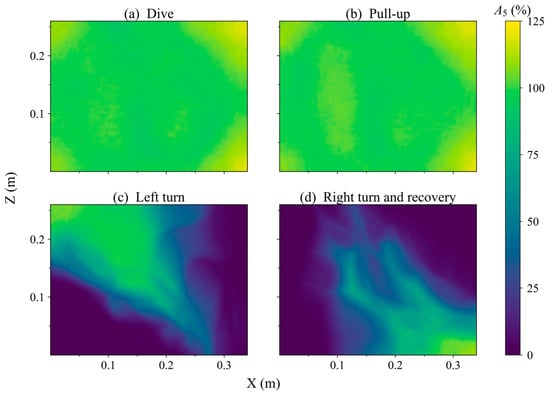
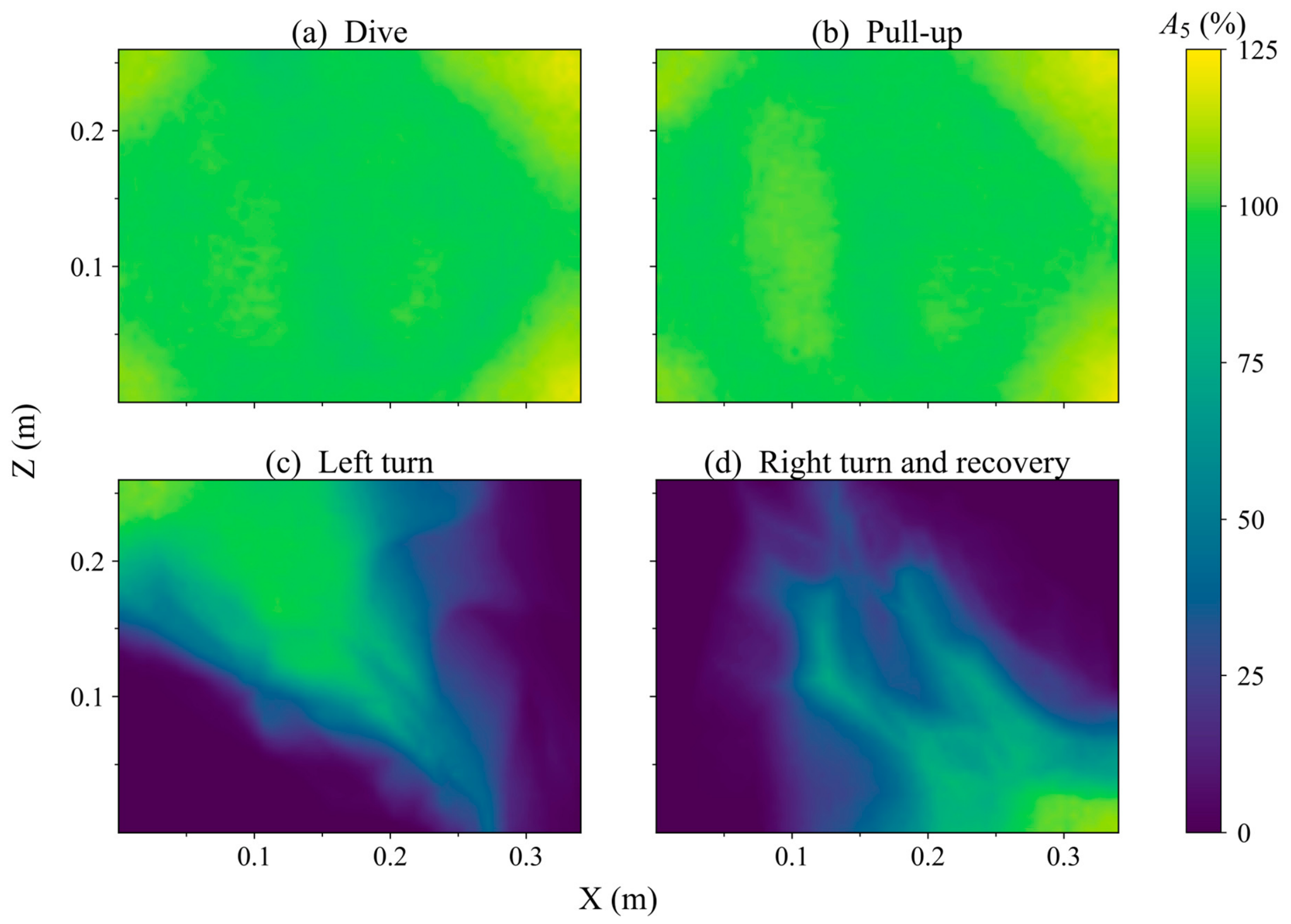
To further investigate the stage-dependent variation in local lubricant distribution during continuous maneuvering, the 10 L no-baffle case is selected as a representative condition. Low-percentile availability A₅ is compared among the dive, pull-up, left-turn, and right-turn-and-recovery stages, as shown in Figure 17. During the dive and pull-up stages, A₅ generally remains relatively high, with a comparatively uniform bottom distribution and limited spatial variation. Locations satisfying A₅ ≥ 50% cover the entire effective bottom in both stages.

Figure 17. Spatial distributions of A₅ during different maneuvering stages for the representative 10 L no-baffle case. The color scale spans 0–125%. (a) Dive; (b) pull-up; (c) left-turn; (d) right-turn-and -recovery.

After the turning stages begin, the spatial non-uniformity of A₅ becomes more pronounced. During the left-turn, high- and low-availability regions form an inclined pattern across the bottom. During the subsequent right-turn-and-recovery, the low-value region shifts further, producing substantial differences among bottom locations. The area proportions satisfying A₅ ≥ 50% decrease to 35.04% during the left-turn and 21.63% during the right-turn-and-recovery. For this representative case, turning and attitude recovery are therefore the principal stages in which extensive local low-oil regions develop.

The low-value regions formed in different maneuvering stages do not completely overlap, indicating that unfavorable local lubricant locations depend on the stage. After a transition, the distribution established in the preceding stage continues to adjust to the new motion, so a location with high availability in one stage may still experience low-oil conditions later. Evaluation of a single stage therefore cannot fully characterize the local lubricant state throughout continuous maneuvering. Candidate locations must satisfy the A₅ requirement in all four stages and the complete-period A_min and L₅₀ conditions. For this representative case, the area satisfying all four stage-wise A₅ requirements is 5.29%, smaller than the area passing either turning stage alone.

3.4. Candidate-Region Identification and Oil Suction Port Placement Analysis

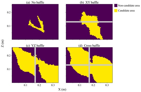
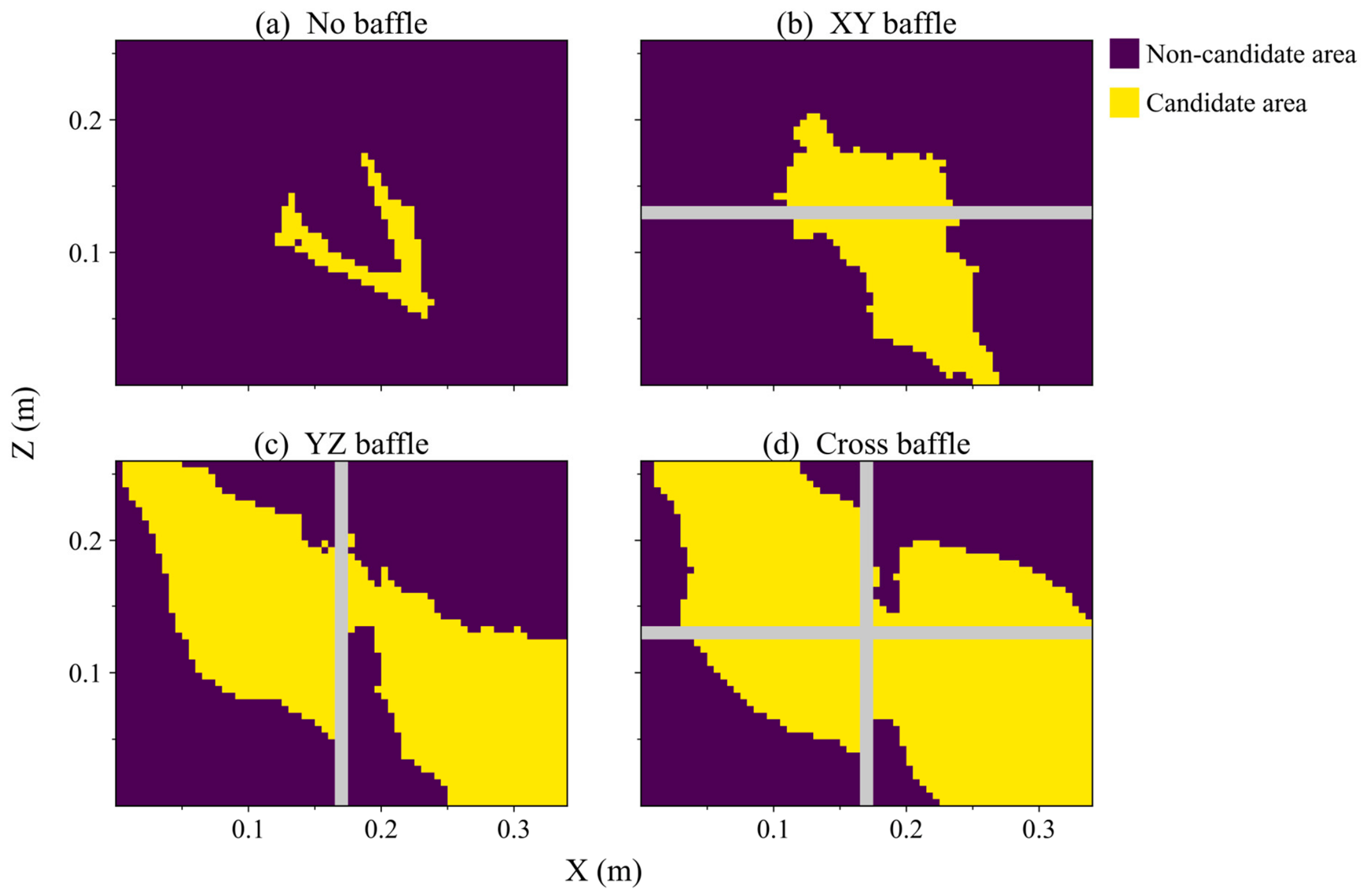
The preceding results show that reducing the initial oil volume contracts the candidate regions satisfying the assessment requirements. Figure 18 presents the joint screening results for 10 L: yellow denotes candidate suction port centers satisfying the criteria, purple denotes locations that fail, and gray denotes the baffle footprint. The configurations differ in the location, extent, and shape of their candidate regions.

Figure 18. Candidate regions for suction port centers in the four configurations at 10 L. The criteria are A₅ ≥ 50% in each stage, complete-period A_min > 0, and L₅₀ ≤ 0.2 s. (a) No baffle; (b) XY baffle; (c) YZ baffle; (d) cross baffle.

Without baffles, the candidate region is confined to a narrow central area, leaving relatively few placement options. The XY baffle produces local candidate regions on its two sides, while the YZ baffle provides larger regions in both compartments. The cross baffle further changes the bottom lubricant distribution and retains larger candidate regions in multiple compartments, with an area ratio of 59.39%. Under the baseline conditions of this group, all locations passing the combined A₅ and A_min requirements also satisfy L₅₀.

The candidate regions provide a preliminary spatial screening of potential suction port centers, with a larger region offering greater placement flexibility. The final layout should account for suction port dimensions and height, available space, and pipeline routing.

4. Conclusions

This study addresses the quantitative assessment of the local lubricant state and its dynamic variation in an aviation lubricant tank under continuous maneuvering. An SPH-based local lubricant availability assessment is developed using time-resolved particle information. Regularly arranged virtual sampling domains convert transient particle data into local lubricant-availability histories. Low-percentile availability A₅, minimum availability A_min, and the longest continuous low-oil duration L₅₀ describe the overall level, extreme state, and continuous low-oil duration, respectively. Their joint application screens candidate regions for suction port centers and translates transient lubricant migration into spatial guidance for port placement.

Within the conditions investigated, the initial oil volume and internal baffle configuration affect the local lubricant state and candidate-region distribution. As the initial oil volume decreases, local low-oil conditions become more likely, candidate regions satisfying the screening criteria contract, and differences among baffle configurations become more pronounced. At 10 L, the candidate-region area ratios are 4.19% for the no-baffle configuration and 59.39% for the cross-baffle configuration.

Different baffle layouts redirect lubricant migration and redistribution, producing distinct candidate-region patterns at low initial oil volumes. A₅, A_min, and L₅₀ describe different aspects of the local lubricant state, and their spatial responses need not coincide. Some configurations improve the overall lubricant distribution, yet sustained low-oil events may persist within certain compartments. Internal structures should therefore be assessed using both the local lubricant level and its temporal characteristics near potential suction locations.

For the representative 10 L no-baffle case, extensive local low-oil regions develop during turning and attitude recovery, and the low-value locations differ among stages. A single time point or an overall distribution measure cannot fully characterize the local lubricant variation throughout the maneuver. The proposed stage-wise, multi-metric assessment accounts for conditions in the different stages and supports candidate-location screening under continuous maneuvering.

The candidate regions identified in this study provide a quantitative reference for preliminary spatial screening of potential suction port centers under the evaluated conditions. In practical design, the final location should be selected within a candidate region while accounting for baffle positions, tank boundaries, suction-pipeline routing, installation space, and other structural constraints. No actual suction flow is imposed in the present model. Further assessment incorporating the inlet geometry and supply requirements is therefore needed to evaluate inlet pressure, supply flow rate, air ingestion, vortices, and other aspects of suction performance.

References

- Hu, X.; Wang, A.; Li, P.; Wang, J. Influence of dynamic attitudes on oil supply for bearings and churning power losses in a splash lubricated spiral bevel gearbox. Tribol. Int. 2021, 159, 106951. [Google Scholar] [CrossRef] [Scilit]
- Yang, J.; Shao, S.; Zhang, K.; Liu, Y.; Cao, G. Flow field study and lubrication performance optimization of gearbox based on the SPH method. J. Braz. Soc. Mech. Sci. Eng. 2025, 47, 338. [Google Scholar] [CrossRef] [Scilit]
- Chintala, P.; Inada, J.; Flores Solano, C.A.; Gingade, S. Advancing Electric Drive Unit Design with Smoothed Particle Hydrodynamics. In Proceedings of the WCX SAE World Congress Experience 370157, Detroit, MI, USA, 14–16 April 2026. [Google Scholar] [CrossRef] [Scilit]
- Wang, Y.; Ruan, C.; Lu, S.; Li, Z. A Study on the Movement Characteristics of Fuel in the Fuel Tank during the Maneuvering Process. Appl. Sci. 2023, 13, 8636. [Google Scholar] [CrossRef] [Scilit]
- Fontanesi, S.; Olcuire, M.; Cicalese, G.; Lamberti, L.; Pulvirenti, F.; Berni, F. Computational Fluid Dynamics (CFD) Analysis of Lubricant Oil Tank Sloshing of a High-Performance Car under Racetrack Maneuvers. SAE Int. J. Engines 2022, 15, 185–201. [Google Scholar] [CrossRef] [Scilit]
- Constantin, L.; De Courcy, J.J.; Titurus, B.; Rendall, T.C.S.; Cooper, J.E.; Gambioli, F. Effect of Fuel Sloshing on the Damping of a Scaled Wing Model—Experimental Testing and Numerical Simulations. Appl. Sci. 2022, 12, 7860. [Google Scholar] [CrossRef] [Scilit]
- Erzan Topçu, E.; Kılıç, E. A Numerical Investigation of Sloshing in a 3D Prismatic Tank with Various Baffle Types, Filling Rates, Input Amplitudes and Liquid Materials. Appl. Sci. 2023, 13, 2474. [Google Scholar] [CrossRef] [Scilit]
- Al-Yacouby, A.M.; Ahmed, M.M. A Numerical Study on the Effects of Perforated and Imperforate Baffles on the Sloshing Pressure of a Rectangular Tank. J. Mar. Sci. Eng. 2022, 10, 1335. [Google Scholar] [CrossRef] [Scilit]
- Wang, Q.; Qi, W.; Zheng, G.; Xu, W.; Yu, H. Liquid sloshing in a tank vehicle: A numerical and experimental investigation with baffle configurations. Measurement 2024, 234, 114806. [Google Scholar] [CrossRef] [Scilit]
- Lu, T.; Cao, D. Comparative study on wave response to vertical baffle orientation for resonant sloshing suppression in an upright cylindrical tank. Ocean Eng. 2025, 341, 122526. [Google Scholar] [CrossRef] [Scilit]
- Rubesh Raja, V.; Palanisamy, P. A numerical study of wave baffles on sloshing reduction of rectangular containers under combined excitation. Mech. Adv. Mater. Struct. 2024, 31, 11561–11578. [Google Scholar] [CrossRef] [Scilit]
- Zhang, N.; Pan, S.; Liu, J.; Liu, M.; Wang, W. CFD Study of Lubrication Pump Starvation Due to Oil Pan Sloshing. In Proceedings of the KSAE/SAE 2025 Powertrain, Energy & Lubricants Conference & Exhibition 361994, Busan, Republic of Korea, 22–25 June 2025. [Google Scholar] [CrossRef] [Scilit]
- Wang, L.; Liu, Y.; Zhang, K.; Yao, Y.; Shao, S.; He, K. Study of Lubrication Performance and Churning Loss under Mixed Lubrication Mode in Gearbox. Lubricants 2024, 12, 283. [Google Scholar] [CrossRef] [Scilit]
- Boniou, V.; Schmitt, T.; Vié, A. Comparison of interface capturing methods for the simulation of two-phase flow in a unified low-Mach framework. Int. J. Multiph. Flow 2022, 149, 103957. [Google Scholar] [CrossRef] [Scilit]
- Gibou, F.; Fedkiw, R.; Osher, S. A review of level-set methods and some recent applications. J. Comput. Phys. 2018, 353, 82–109. [Google Scholar] [CrossRef] [Scilit]
- Mahfoze, O.A.; Liu, W.; Longshaw, S.M.; Skillen, A.; Emerson, D.R. On the Efficacy of Turbulence Modelling for Sloshing. Appl. Sci. 2022, 12, 8851. [Google Scholar] [CrossRef] [Scilit]
- Monaghan, J.J. Smoothed particle hydrodynamics. Rep. Prog. Phys. 2005, 68, 1703–1759. [Google Scholar] [CrossRef] [Scilit]
- Lind, S.J.; Rogers, B.D.; Stansby, P.K. Review of smoothed particle hydrodynamics: Towards converged Lagrangian flow modelling. Proc. R. Soc. A 2020, 476, 20190801. [Google Scholar] [CrossRef] [Scilit]
- Pozorski, J.; Olejnik, M. Smoothed particle hydrodynamics modelling of multiphase flows: An overview. Acta Mech. 2024, 235, 1685–1714. [Google Scholar] [CrossRef] [Scilit]
- Wang, Z.-B.; Chen, R.; Wang, H.; Liao, Q.; Zhu, X.; Li, S.-Z. An overview of smoothed particle hydrodynamics for simulating multiphase flow. Appl. Math. Model. 2016, 40, 9625–9655. [Google Scholar] [CrossRef] [Scilit]
- Vacondio, R.; Altomare, C.; De Leffe, M.; Hu, X.; Le Touzé, D.; Lind, S.; Marongiu, J.-C.; Marrone, S.; Rogers, B.D.; Souto-Iglesias, A. Grand challenges for smoothed particle hydrodynamics numerical schemes. Comput. Part. Mech. 2021, 8, 575–588. [Google Scholar] [CrossRef] [Scilit]
- O’Connor, J.; Rogers, B.D. A fluid–structure interaction model for free-surface flows and flexible structures using smoothed particle hydrodynamics on a GPU. J. Fluids Struct. 2021, 104, 103312. [Google Scholar] [CrossRef] [Scilit]
- Haftu, A.; Muta, A.; Ramachandran, P. Parallel adaptive weakly-compressible SPH for complex moving geometries. Comput. Phys. Commun. 2022, 277, 108377. [Google Scholar] [CrossRef] [Scilit]
- Sun, X.; Zhong, Y.; Bian, F.; Liu, C.; Yin, Y. Numerical Computation of Sloshing-Induced Force in Complex Ship Tanks under the Excitation of Ship Rolling Motion Based on the MPS Method. Appl. Sci. 2022, 12, 5130. [Google Scholar] [CrossRef] [Scilit]
- Lu, T.; Cao, D. SPH study of sloshing dynamics and energy dissipation characteristics in baffled tanks with varying baffle quantities. Ocean Eng. 2025, 340, 122378. [Google Scholar] [CrossRef] [Scilit]
- Bender, J.; Koschier, D. Divergence-Free SPH for Incompressible and Viscous Fluids. IEEE Trans. Vis. Comput. Graph. 2017, 23, 1193–1206. [Google Scholar] [CrossRef] [Scilit]
- Ansys Inc. Rocky SPH Technical Manual, Release 2026 R1; Ansys Inc.: Canonsburg, PA, USA, 2026; Available online: https://ansyshelp.ansys.com/public/Views/Secured/corp/v261/en/dem_sph_tec/DFSPH.html (accessed on 7 October 2026).
- Lucy, L.B. A numerical approach to the testing of the fission hypothesis. Astron. J. 1977, 82, 1013–1024. [Google Scholar] [CrossRef] [Scilit]
- Gingold, R.A.; Monaghan, J.J. Smoothed particle hydrodynamics: Theory and application to non-spherical stars. Mon. Not. R. Astron. Soc. 1977, 181, 375–389. [Google Scholar] [CrossRef] [Scilit]
- Monaghan, J.J. Simulating free surface flows with SPH. J. Comput. Phys. 1994, 110, 399–406. [Google Scholar] [CrossRef] [Scilit]
- Morris, J.P.; Fox, P.J.; Zhu, Y. Modeling low Reynolds number incompressible flows using SPH. J. Comput. Phys. 1997, 136, 214–226. [Google Scholar] [CrossRef] [Scilit]
- Cleary, P.W. Modelling confined multi-material heat and mass flows using SPH. Appl. Math. Model. 1998, 22, 981–993. [Google Scholar] [CrossRef] [Scilit]
- Brown, S.; Colville, S.; Lee, Y.; Greaves, D. Isothermal Sloshing in a Circular Tank (CCP-WSI Test Case 017 Dataset); University of Plymouth Research Repository: Plymouth, UK, 2025. [Google Scholar] [CrossRef]
- Brown, S.A.; Colville, S.W.; Francis, V.; Zhao, T.; Lee, Y.C.; Cao, D.; Chen, H.; Chen, J.; Chen, S.; Davidson, J.; et al. A blind comparative study on isothermal sloshing in a circular tank (CCP-WSI Blind Test Series 5). Ocean Eng. 2026, 362, 126290. [Google Scholar] [CrossRef] [Scilit]
- Shell. AeroShell Turbine Oil 555: Technical Data Sheet, Version 1.3; Royal Dutch Shell: London, UK, 2020; Available online: https://www.shell-livedocs.com/data/published/en/eab103ba-927d-4d68-97d4-f1008d707f50.pdf (accessed on 4 November 2026).
Disclaimer/Publisher’s Note: The statements, opinions and data contained in all publications are solely those of the individual author(s) and contributor(s) and not of MDPI and/or the editor(s). MDPI and/or the editor(s) disclaim responsibility for any injury to people or property resulting from any ideas, methods, instructions or products referred to in the content. |
© 2026 by the authors. Licensee MDPI, Basel, Switzerland. This article is an open access article distributed under the terms and conditions of the Creative Commons Attribution (CC BY) license.