


Abstract
We investigate the fundamental kinematic parameters of stellar motions in the Milky Way using a statistical sample of 27,485,720 stars with measured three-dimensional velocities from the Gaia DR3 catalogue. From these data, we determine the local solar velocity , the average rotation velocity km/s, and the circular velocity km/s, both at the radius . Next, within the range of kpc, we derive the Galactic circular velocity curve and determine the average spherical components of the stellar velocities as functions of both Galactocentric radius R and distance from the Galactic plane . Two-dimensional maps of these components reveal a complex three-dimensional kinematic structure. In particular, the pattern observed at kpc can be associated with the influence of the Galactic bar. To facilitate the description of the observations, we employ a simplified axisymmetric Monte Carlo model with several free parameters that reproduces the main kinematic trends.
1. Introduction
The Milky Way (MW) represents a unique laboratory for studying gravity and for understanding the formation and evolution of galaxies. In recent years, the Gaia space observatory has provided an unprecedented amount of highly precise astrometric, photometric, and spectroscopic data for millions of stars in the MW [1]. The scientific exploitation of these data has led to thousands of studies devoted to Galactic structure, stellar populations, and Galactic dynamics.
In particular, the Gaia DR3 catalogue provides exceptionally rich input data for constructing a detailed kinematic map of the MW, far beyond what was previously achievable. These data reveal structures on a broad range of spatial and dynamical scales, from gravitationally bound binaries and multiple stellar systems [2,3] to streaming motions associated with spiral arms [4,5], local velocity fluctuations and turbulence, and the global rotation of the Galactic disk and halo.
The observed Galactic rotation strongly suggests the presence of dark matter, which is believed to constitute a substantial fraction of the total mass of the MW (see [6,7,8,9,10,11,12,13,14,15,16,17] and the overview in [18]). Recent analyses of MW kinematics have provided increasingly accurate determinations of the Galactic circular velocity curve, defined as the radial dependence of the galaxy circular velocity [7,15,19,20,21,22]. Circular velocity curves represent one of the principal observational constraints for models of Galactic mass distribution and dark matter halos.
In addition to gravity, the formation and evolution of stars are governed by the forces of the microworld, namely the strong and electroweak interactions described by the Standard Model of particle physics. However, despite extensive observational and theoretical efforts, the microscopic nature and origin of dark matter remain unresolved.
Another important area of current research concerns the detailed mapping of kinematic substructures and deviations from axial symmetry within the MW, including spiral-arm perturbations, resonances induced by the Galactic bar, phase-space streams, and vertical oscillatory motions [20,23,24,25,26,27,28,29,30,31]. A comprehensive overview of the integrated, structural, and kinematic properties of the Galaxy is provided in [32].
In general, the kinematic structure of galaxies also provides important clues to their evolutionary history. Observations have revealed galaxies with unusual kinematic properties, suggesting that their disks may have undergone significant changes over time. Such evolutionary processes could result in an atypical orientation of the galactic disk with respect to the dark matter halo. Previous studies have generally indicated an alignment between the angular momentum of dark matter and that of the baryonic component of galaxies [33,34,35,36,37]. Departures from this general picture may arise from interactions with smaller galaxies, including mergers or accretion events involving a more massive host galaxy. The MW itself may have experienced such interactions, and certain perturbations in its kinematic structure could provide observational evidence of these past events.
The primary objective of this paper is to derive the circular velocity curves of the MW using data from the Gaia observatory, specifically a subset of sources with measured radial velocities from the DR3 catalogue [38]. These data enable a complete 3D reconstruction of stellar kinematics in arbitrary coordinate systems. Our analysis focuses on the distribution of stellar velocity components in spherical coordinates and on their dependence on spatial position. This work extends our previous 2D kinematic analysis based on the full DR3 catalogue, in which sources lacking radial velocity measurements constitute the dominant fraction of the dataset [39].
Section 2 introduces the basic concepts and variables used throughout the study. Section 3 describes the criteria used for selecting stars and defines the angular sectors of the Galactic system that are suitable for separate analysis. A useful tool for modelling derived velocity distributions is a simple Monte Carlo (MC) simulation with several free parameters, the algorithm for which is described in Section 4. Essentially, the same model was employed in our earlier 2D analysis; however, the present 3D approach enables a more precise determination of the free parameters.
The results are presented in Section 5. In addition to circular velocity curves, our analysis also provides more general velocity maps in coordinates. The accuracy of these results depends crucially on the precise determination of the Sun’s motion, which coincides with the motion of the Gaia observatory. The independent calculation of the Sun’s local velocity and the Galaxy’s mean rotational velocity at the radius of the Sun’s orbit is an important part of our analysis. In Section 6, the results obtained are discussed and, where appropriate, compared with the results of previous studies.
2. Definition of Variables
The positions of sources in Gaia data are expressed in galactic angular coordinates: longitude (l) and latitude (b). Using parallax, we can also define the distance ( of the source from the Sun. The proper motion of the stars in Gaia data is represented by the vector
whose components are angular velocities in the directions of right ascension and declination in the ICRS. For our analysis, we prefer the representation of proper motion in the galactic reference frame:
which is obtained by the transformation given in [40]. Then, the transverse 2D velocity defined as
where are velocity components in directions of increasing latitude and longitude , and the distance r is obtained from the parallax p:
where ZP is the value of the parallax zero-point for Gaia EDR3 and Gaia DR3 returned by the Python gaiadr3_zeropoint package [41] based on the functions described in [42]. We work with data that also include radial velocity (), so we have complete 3D data on position and velocity relative to the Sun’s position. For our analysis, it is convenient to express spherical components in the local standard of rest (LSR) frame. In fact, there are two LSR approaches:
- (i)
- Kinematic—based on the average motion of nearby stars. The key parameter is , the average velocity of the stars along the circular path of radius .
- (ii)
- Dynamic—a hypothetical point that would orbit the Galaxy along a perfectly circular path at a given distance from the Galactic centre. The key parameter is , the circular velocity of this point along the path of radius .
In the first step, the analysis is conducted within a kinematic framework. Subsequently, in Section 5, selected results are appropriately corrected to account for the effects associated with the dynamic formulation.
If is the Sun’s velocity relative to the average velocity of the surrounding stars, then the corresponding LSR components take the form
and satisfy
independently in various sectors around the Sun. The practical application of this definition is demonstrated in Section 5. The resulting may, of course, depend to some extent on the choice of these sectors. This inevitable uncertainty must be included in the measurement error. The vectors define directions of increasing coordinates . In terms of Cartesian coordinates, we have
In the next step, we transform spherical galactic LSR coordinates and velocities to the Galactocentric representation:
where
The explicit forms of the unit vectors and are given in Appendix A, where the relationship between galactic and Galactocentric coordinates is defined. For clarity, we use the following convention throughout the paper: positions, velocities, and their coordinates are denoted in lowercase (uppercase) in the galactic (Galactocentric) reference frame. The LSR frame rotates around the Galactic centre, so the total Galactocentric velocity reads
where velocity is defined as the average rotation velocity of stars in the Galactic plane and at the radius of the Sun’s orbit . For our analysis, we use the value kpc [43]. The rotation velocity of a star reads
The direction of increasing (or ) is opposite to the direction of the Galaxy’s rotation, which explains the negative value of see Figure A1 in Appendix A.
The velocities are the subject of statistical analysis. The function
averaged in the galactic plane at fixed R is the input for the calculation of the circular velocity curve . Velocity defined above is a special case: The rotation curve reflects the collective rotation velocity rather than the velocity of a test particle [11]. We also study the functions and depending on two cylindrical coordinates (A5). The average denotes the average value in the corresponding bin centred at the point .
3. Dataset
The data sectors of the sky used for analysis are defined in Table 1.
Table 1.
Sectors of the sky and the number of stars in them. The sectors N0, Q0 and S0 cover the entire range of l: .
From the set of all Gaia DR3 sources with a defined radial velocity (33,812,183 stars) [38], we only accept sources with a positive parallax p and limited distance kpc that satisfy the following condition:
where we use the relation [39]
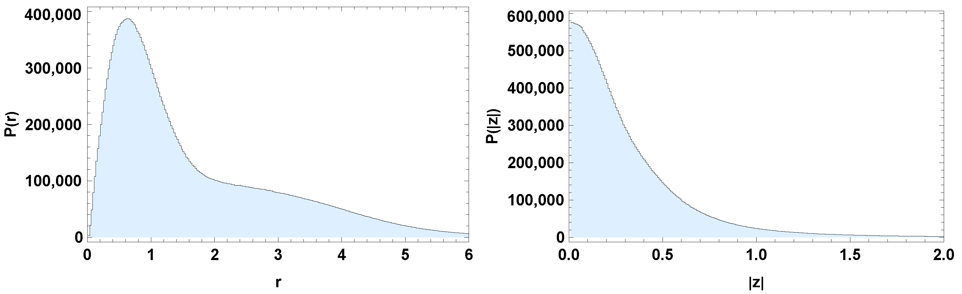
All parameters, including errors, are included in the Gaia DR3 data. The resulting star counts are listed in the table. After these cuts, we are left with a total of 27,485,720 stars for further analysis. The distributions of their distances from the Sun and from the galactic plane over all sectors are shown in Figure 1.
Figure 1.
Distribution of distances from the Sun (left) and from the galactic plane (right). Units: [kpc]. Bin widths: 0.024 and 0.008 kpc.
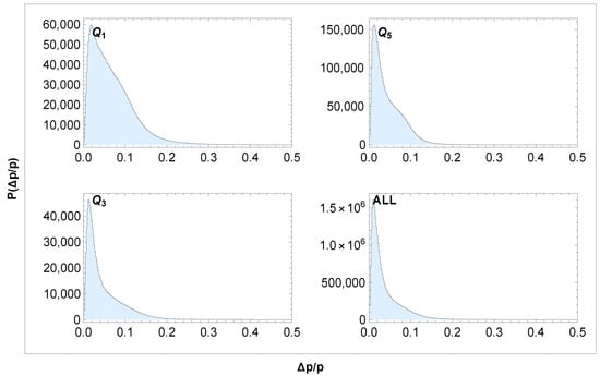
Note that the cuts (13) simultaneously select sources with higher parallax precision. Figure 2 show the corresponding distribution of relative parallax errors. The selected sources meet the condition in all sectors, which is the standard criterion for selecting “good” sources. The first cut on in Equation (13) should be regarded as approximate because covariance terms are neglected in (14). We have verified that the narrowing of the cuts does not systematically affect the parameters of the resulting curves in Section 5. Most of our calculations focus on mean values, which means that the resulting errors are much smaller than the errors of individual entries. The error bars in the figures in Section 5 represent the statistical errors of the average values in the corresponding bins. These errors are calculated using the formula
where is the standard deviation of the velocities and is their number in the given bin.
Figure 2.
Distribution of relative parallax errors across different sectors. Bin width: 0.002.
4. Algorithm of Monte Carlo Simulations
The velocity distributions are compared with a simple MC probabilistic model proposed in our previous study [39]. This model represents an axially symmetric approximation corresponding to a simplified scenario in which local velocity fluctuations are averaged out. The simulated velocity of a star in the Galactocentric reference frame is given by the relation
where the velocity is defined by Equation (12). The components , and are generated in the local reference frame defined by the basis (A6). The model is based on the multinormal distribution
with partial asymmetry (different for positive and negative ). The dependence on R and Z is absorbed in the standard deviations . As a first approximation, we assume
where and are free parameters. We have found that the optimal shape of the distribution is slightly asymmetric, with different for the two opposite orientations, where denotes in (against) the direction of rotation:
Thus, only depends on . This asymmetry also reflects the effective deceleration of the collective rotation for larger :
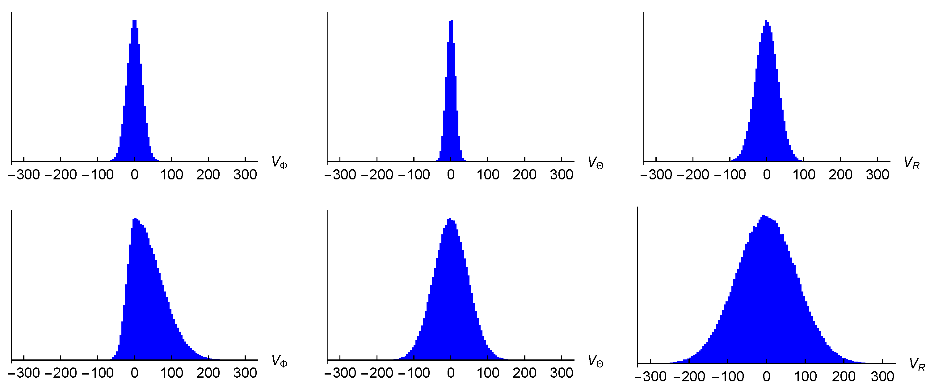
It should be noted that the parameter represents only an average over the sectors and . In Section 5, we show that the actual situation is somewhat more complex. The Wolfram Mathematica code of the generator is available at https://www.fzu.cz/~piska/Catalogue/genkinJUN26.nb (accessed on 8 October 2026). Figure 3 shows examples of the distribution of simulated velocities and . The distributions and are symmetric for any , whereas the distribution is asymmetric for .
Figure 3.
Distribution of simulated velocities , and at (top row) and kpc (bottom row). Units: [km/s].
The simulated distributions at different positions are obtained as follows. The position of the source in the galactic reference frame is transformed using Equation (A3) into the Galactocentric spherical coordinate system . Then, at this position, the velocity is generated according to the distribution (16) using the parameters from Table 2. The optimal parameters listed in the table are obtained through comparison with the real data presented in the following section. The generated velocity can be transformed back to the galactic reference frame:
Table 2.
Optimal parameter values in the MC simulation. Units: , .
In this way, for any source defined by input or , we generate the vector or . To compare the model simulations with the measured data, we also need to know the local velocity of the Sun and the rotation velocity , which we also determine in the following section.
It goes without saying that different methods used to analyse different data samples can lead to slightly different parameters. Since the 3D analysis is more consistent, we give preference to the parameters , and obtained in this work.
5. Results
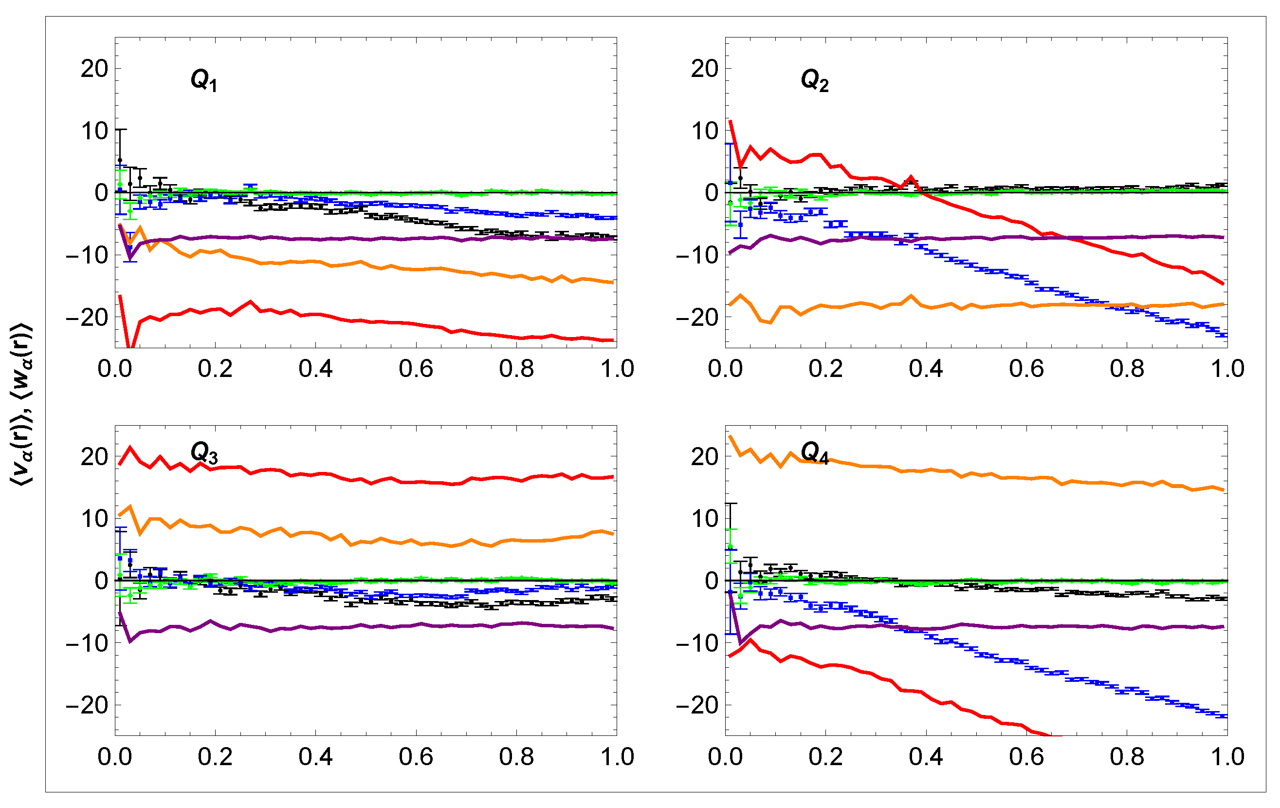
In Figure 4, we show the dependence of average galactic velocities on the distance r. We compare the set of galactic velocities related to the Sun () with those related to the LSR (), defined in Equation (5). Once the Sun’s local velocity has been set correctly, the average velocities should satisfy the condition (6). This condition is well satisfied for the values used in the figure:
Figure 4.
Dependence of mean velocity (blue; green; black; red; purple; and orange) on distance r in sectors –. Units: r [kpc], v [km/s].
These values were obtained after a minor correction (through visual fitting) of our previously measured values in [39], which also includes a comparison with other studies. Since the method for determining is virtually the same in both studies, we adopt the magnitude of systematic errors from the previous study. Statistical errors, on the other hand, are insignificant.
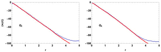
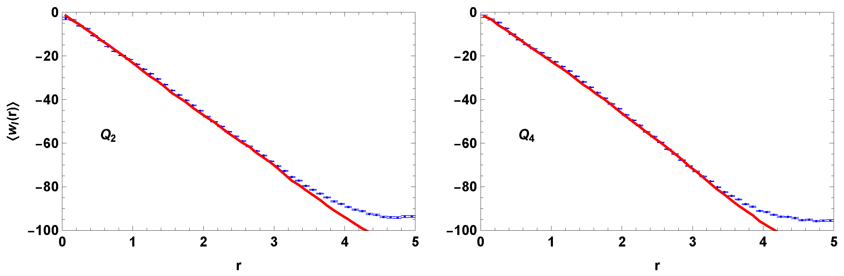
The slope of the curves in sectors and as we discussed in the cited paper, is a direct consequence of MW rotation. In Figure 5, we show these curves on a larger scale together with their simulated counterparts given by Equation (21). Consistency with the simulation further confirms the condition (6) for . The slope can be explained as follows. In the plane of the MW disc , the rotation is defined by the function in (12), so the average velocity at the position observed from the LSR frame reads
Figure 5.
The curves in sectors and : data (blue); simulation model (red). Units: r [kpc], [km/s].
For the curves , we then obtain
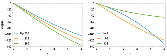
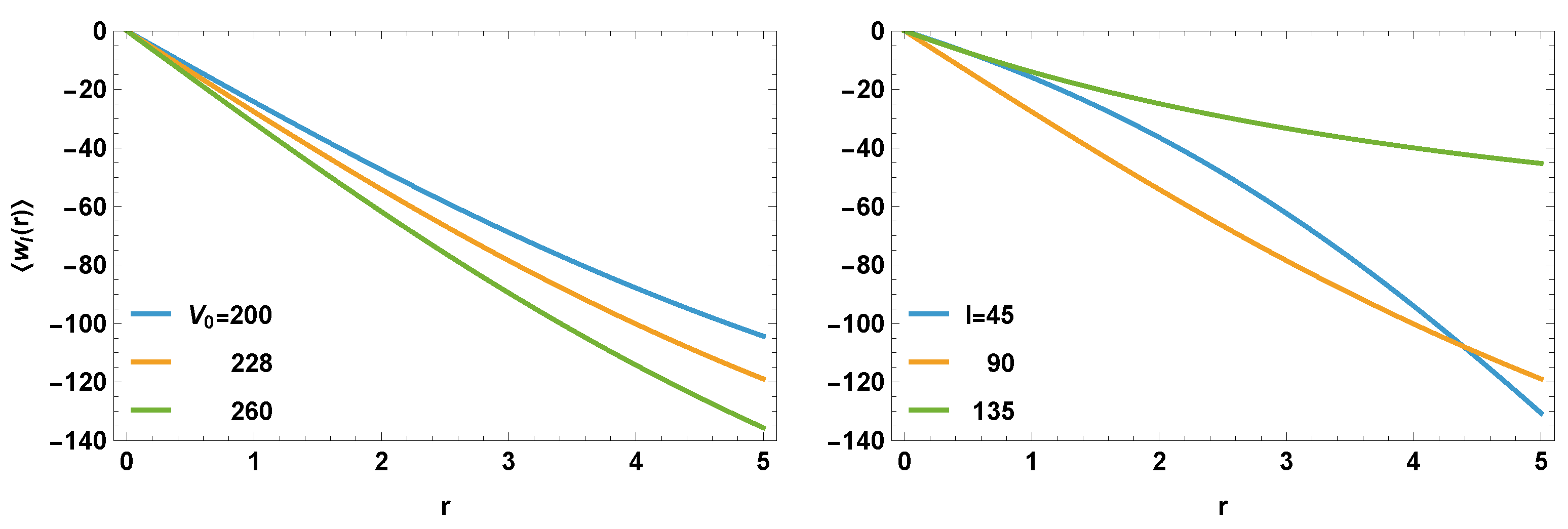
In Figure 6, we show the set of these curves for different values of the parameters and l. The curves in Figure 5 correspond to a superposition of curves over l from the sectors and . The MC simulation is based on the value obtained in the previous study:
Figure 6.
Dependence of velocity on distance r for various rotation velocities (at fixed deg) and various angles l (at fixed km/s) in the galactic plane (). Units: r [kpc], [km/s].
It is clear that agrees perfectly with the measured values in the range kpc, which confirms the previous result.
For consistent comparison with analyses resulting from the dynamic definition of the LSR (see Section 2), the velocities and require a correction based on the calculation of asymmetric drift
where is the MW circular velocity at . The Sun’s rotation velocity in the Galactocentric frame can be decomposed alternatively as
so
In [46], the asymmetric drift around the Sun’s position was estimated to be about 6 km/s. A similar value can be extracted from Figure 3 in [47], where the parameter is replaced with our value of km2s−2, as shown in Table 2. In the standard notation, we can identify
These results are summarised in Table 3.
Table 3.
Sun’s local velocity, mean rotation velocity , and circular velocity . Units: .
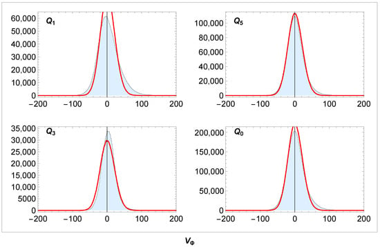
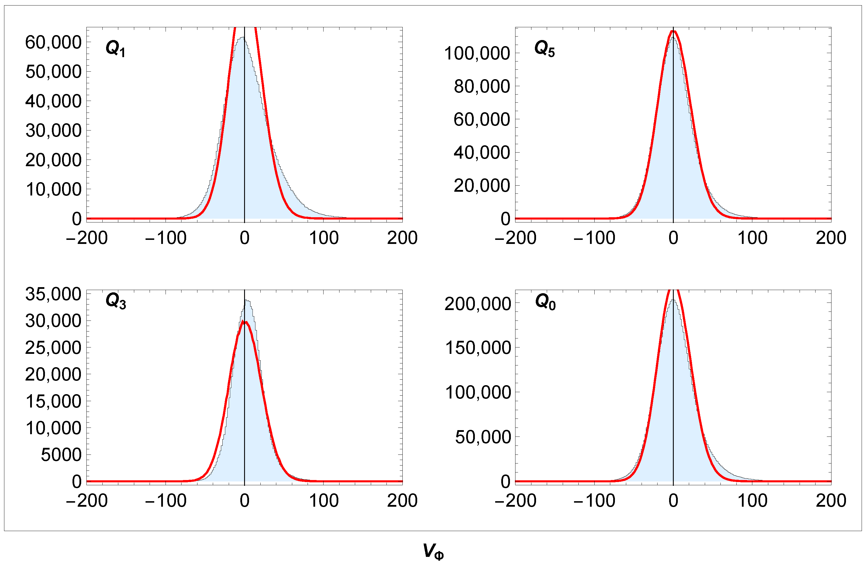
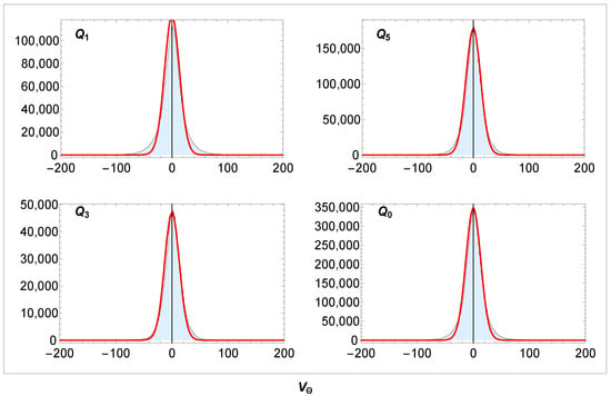
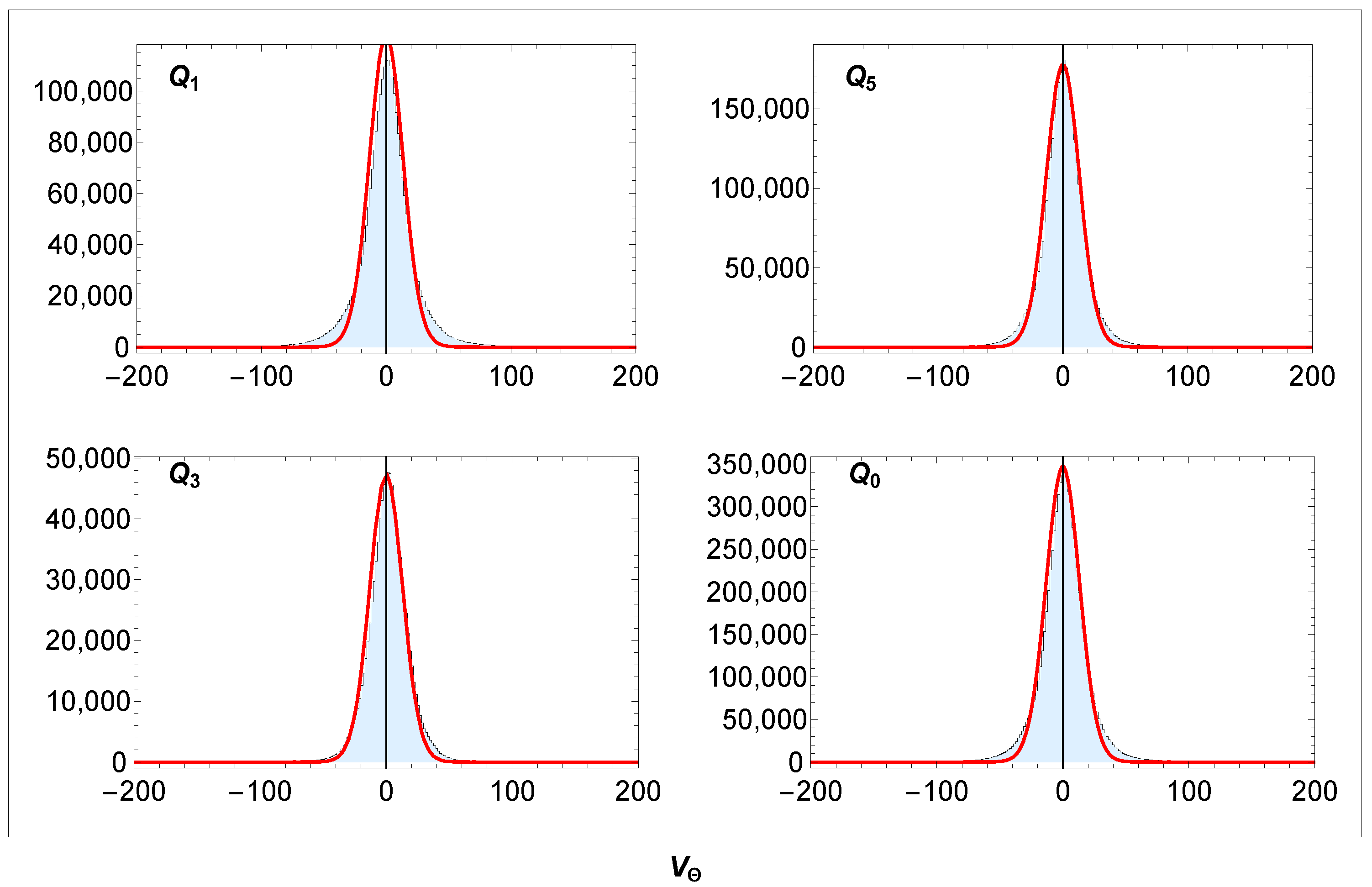
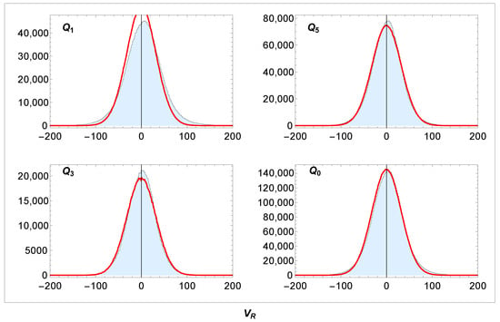
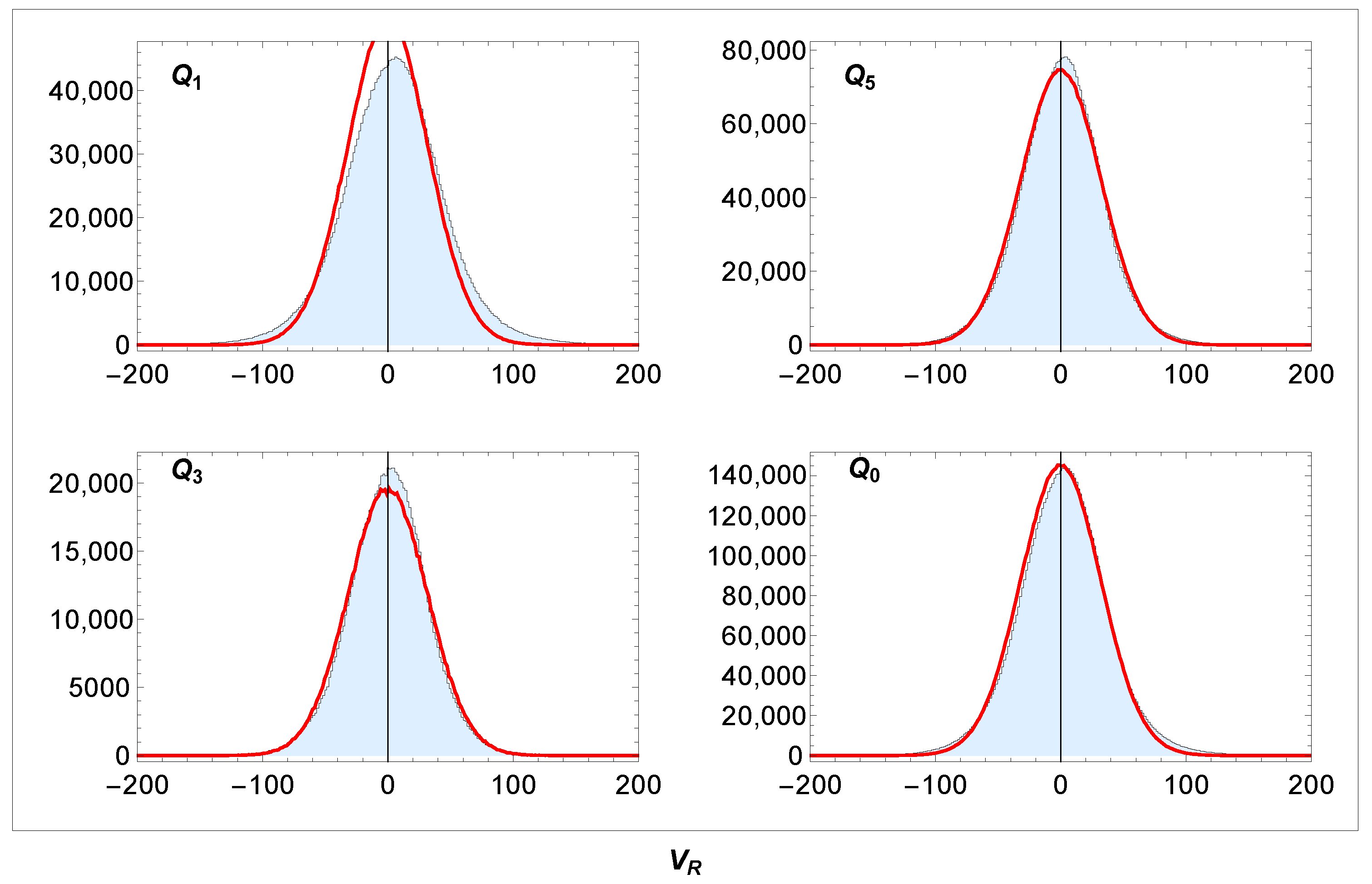
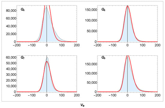
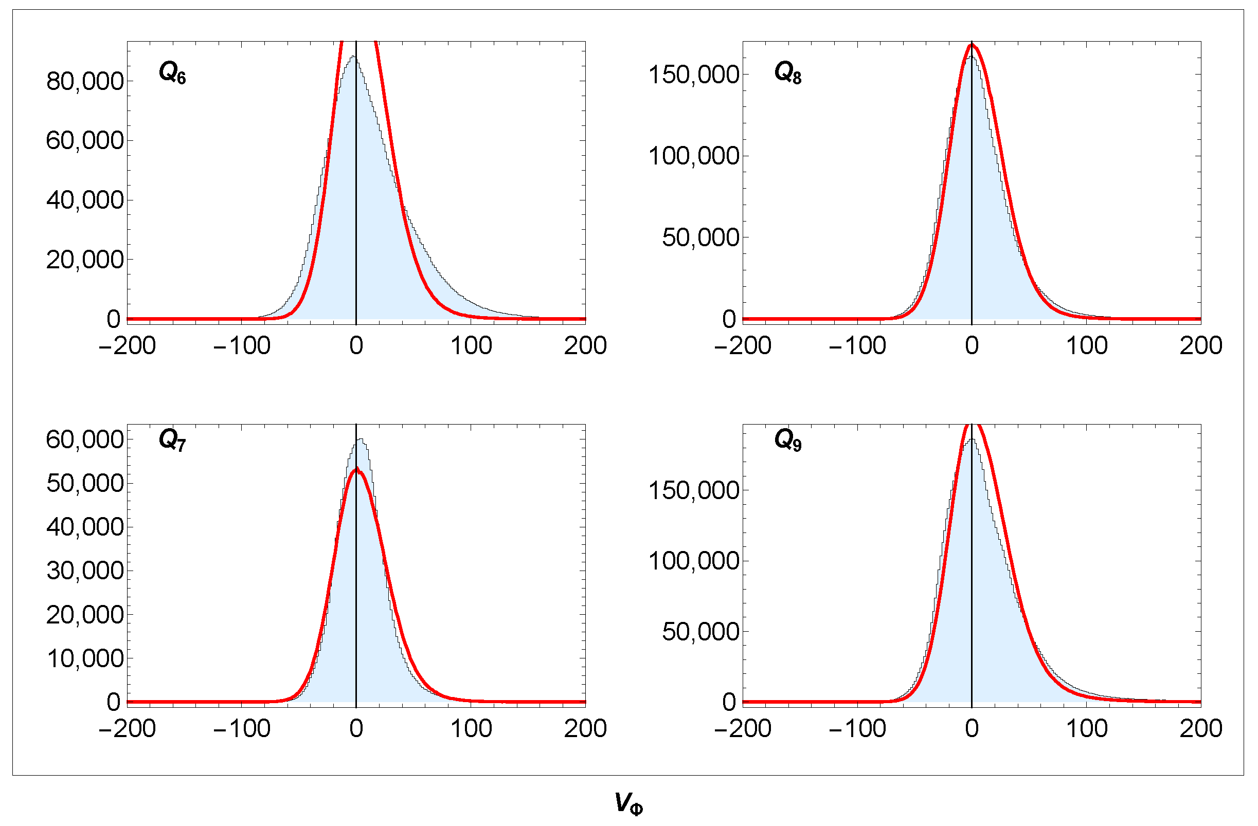
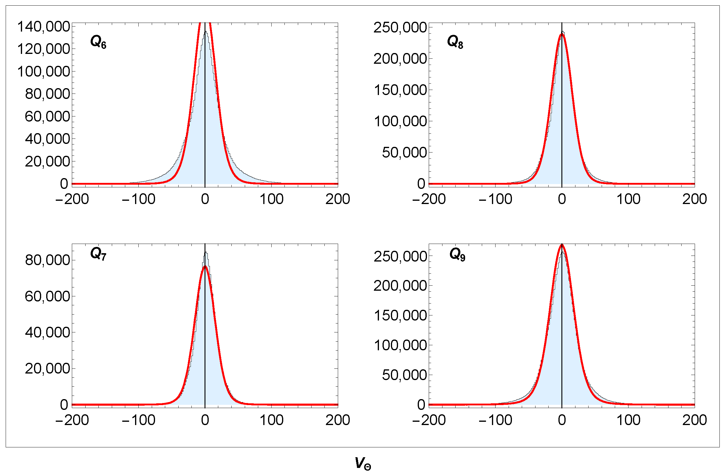
The Galactocentric velocities are calculated using Equation (9). The distributions , and in the sectors – covering the galactic plane are shown in Figure 7, Figure 8 and Figure 9.
The same distributions for other sectors (outside the galactic plane) are shown in Figure 10, Figure 11 and Figure 12. In the figures, we merge the sectors, which, due to rotational symmetry, give very similar results:
Figure 10.
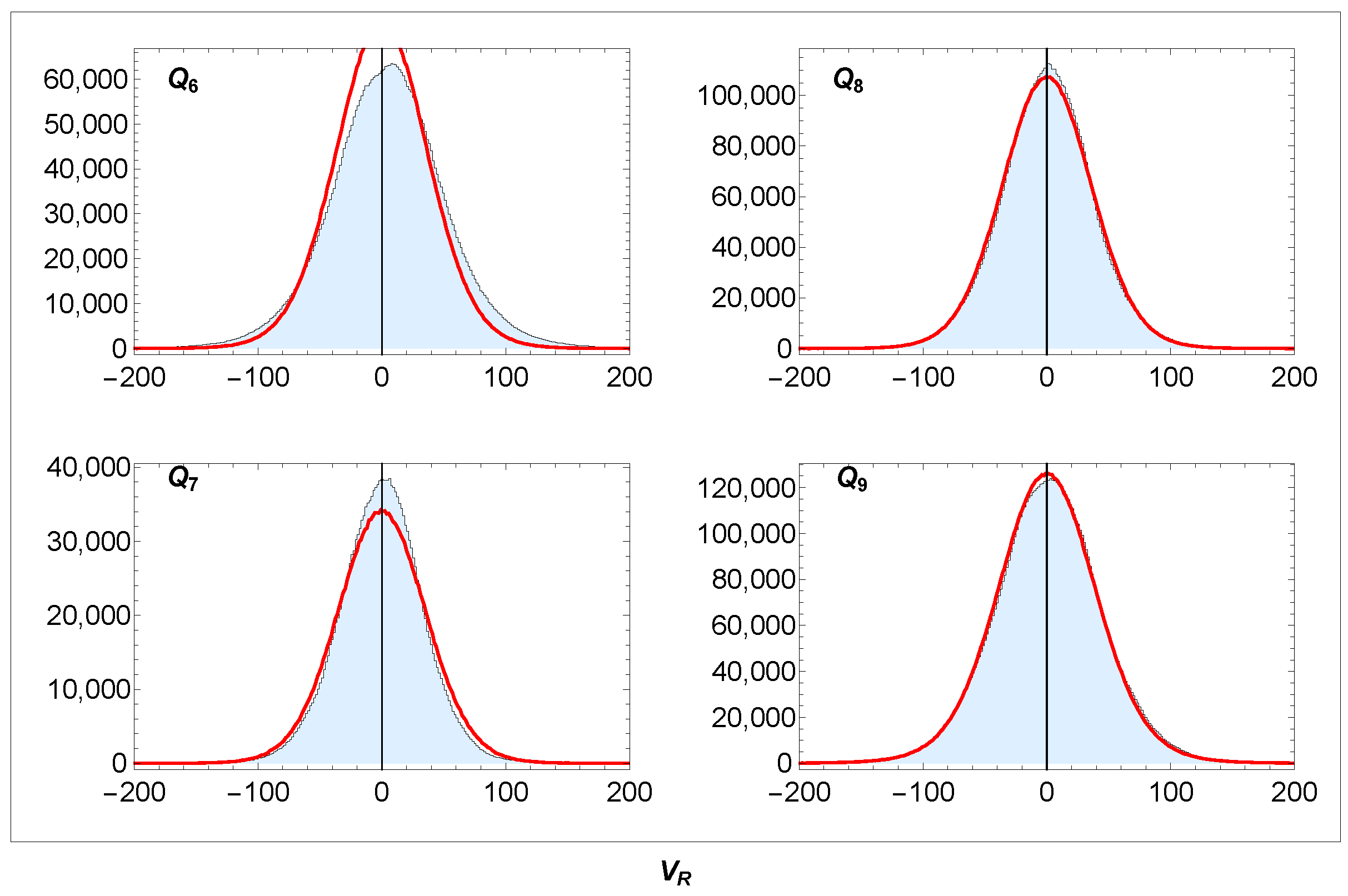
Distributions of in sectors outside the galactic plane defined in Equation (30): data (blue); simulation model (red). Unit: [km/s]. Bin width: 1.6 km/s.
Figure 11.
Distributions of in sectors outside the galactic plane defined in Equation (30): data (light blue) and the simulation model (red). Unit: [km/s]. Bin width: 1.6 km/s.
Figure 12.
Distributions of in sectors outside the galactic plane defined in Equation (30): data (light blue); simulation model (red). Unit: [km/s]. Bin width: 1.6 km/s.
Figure 7, Figure 8, Figure 9, Figure 10, Figure 11 and Figure 12 are used to determine the parameters of the simulated curves in Table 2.
Since these parameters generate 24 different images, we optimised them through visual fitting. The distributions in Figure 7, Figure 8 and Figure 9 correspond to the galactic plane (). Their simulated shapes are controlled solely by the parameters , which are fixed based on these figures. The remaining parameters are then fixed so that the simulation best matches the data in Figure 10, Figure 11 and Figure 12, which correspond to the sectors outside the galactic plane (). In all figures except for sectors and oriented towards the MW centre (), we observe very good agreement between the MC simulation and the data. A slight asymmetry of the distribution (both data and simulation) is observed outside the galactic plane in Figure 10. A slight widening with increasing is most clearly evident in Figure 9 and Figure 12 when comparing the distributions in sectors and . All parameters are close to the values we obtained previously [39] and in other studies listed in the table. In the cited studies, the velocity dispersions are related to the cylindrical coordinate system, whereas ours are related to the spherical one. However, since small values dominate the data, it can be assumed that and correspondingly.
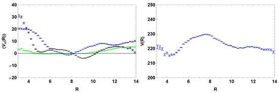
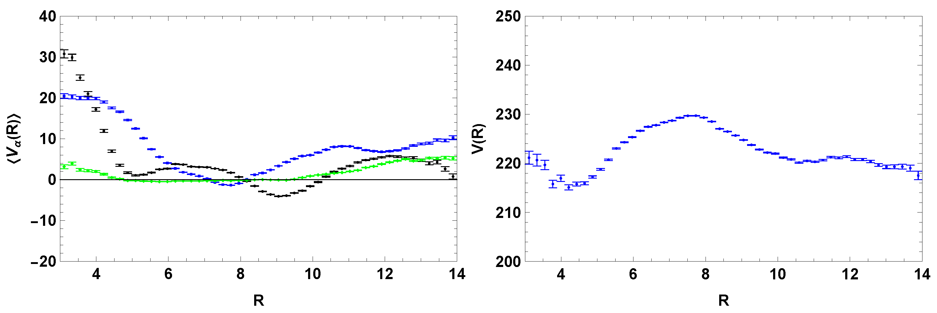
In the left panel of Figure 13, we show the velocity curves , and in sectors covering the galactic plane depending on the radius R in this plane. All curves give zero at the point , which once again confirms the correct setting of in our calculation. The curves fluctuate around zero, while the simulations yield a net zero (not shown in the figure). Local kinematic substructures generate deviations km/s. A more pronounced increase in (which means a decrease in rotation velocity) is evident for kpc. The apparent increase in for kpc may indicate that a slight centrifugal component accompanies the lower rotation velocity in this region. The resulting rotation velocity curve is shown in the right panel, where we used an additional cut deg (see note in the following section). The high number of stars in sector makes it possible to obtain curves with very good resolution of local kinematic substructures.
Figure 13.
Dependence of (blue) (green), and (black) on radius R in the galactic plane (left) in sector Q0 and rotation curve V(R) (right) in the same sector but with an additional cut deg. Units: V [km/s], R [kpc].
Table 4 contains the corresponding circular velocity curve
where, in accordance with [46], the asymmetric drift in the galactic plane is assumed to be km/s regardless of radius R.
Table 4.
Circular velocity curve with corresponding errors in the defined bin. N is the number of entries in a given bin. Units: [km/s], R [kpc].
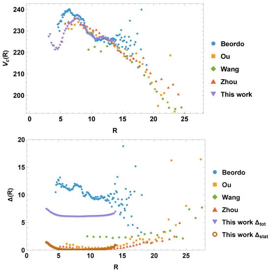
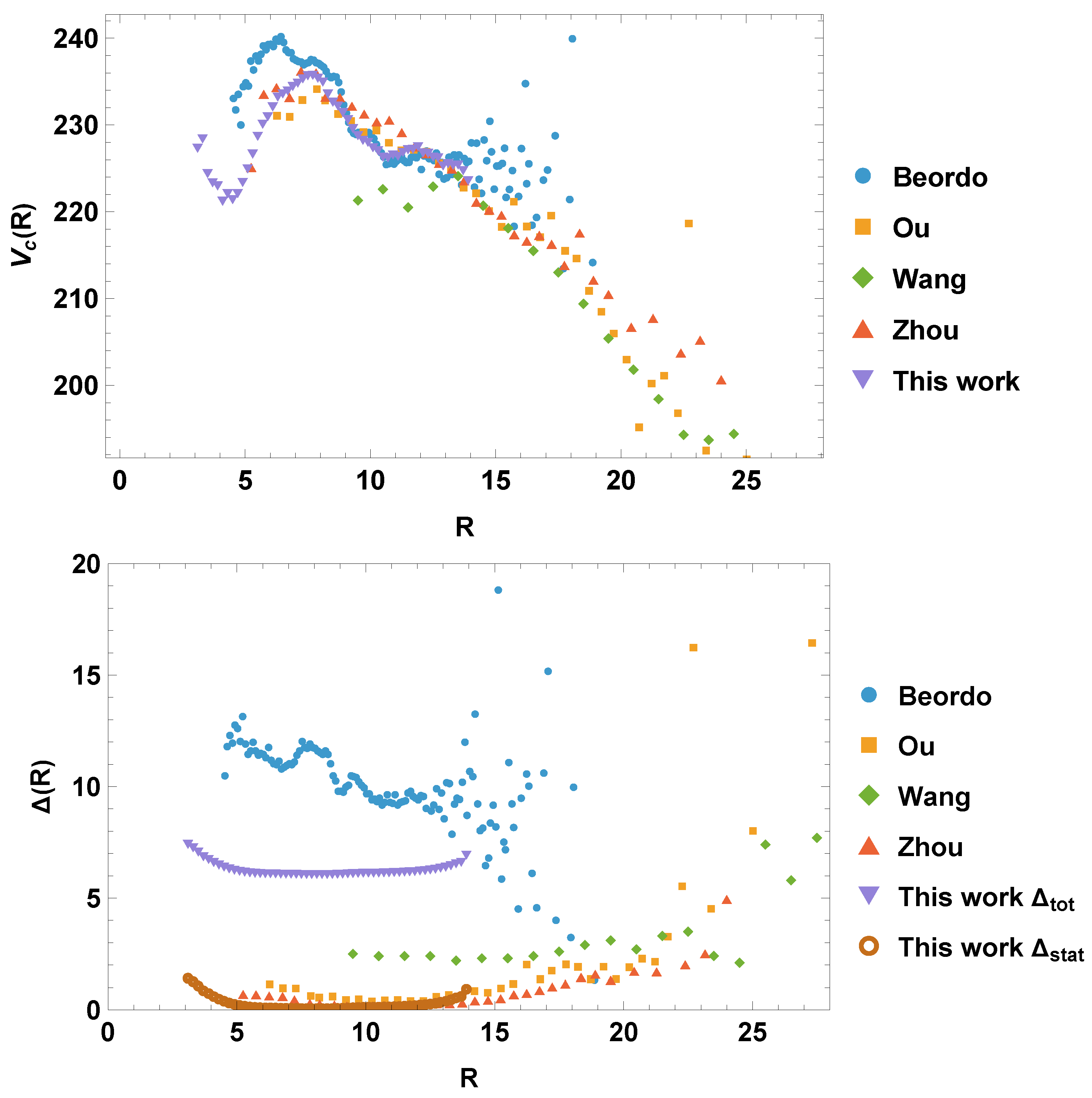
In Figure 14, we show the circular velocity curve together with the results of some other studies. For better clarity, we have illustrated the errors in a separate part.
Figure 14.
Circular velocity curve together with the curves from the studies [7,15,20,21] (top panel) and corresponding errors (bottom panel). Units: [km/s], R [kpc].
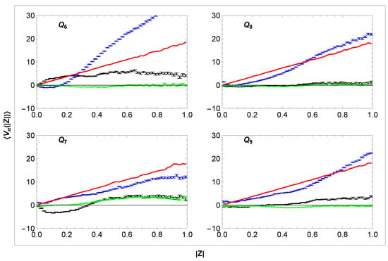
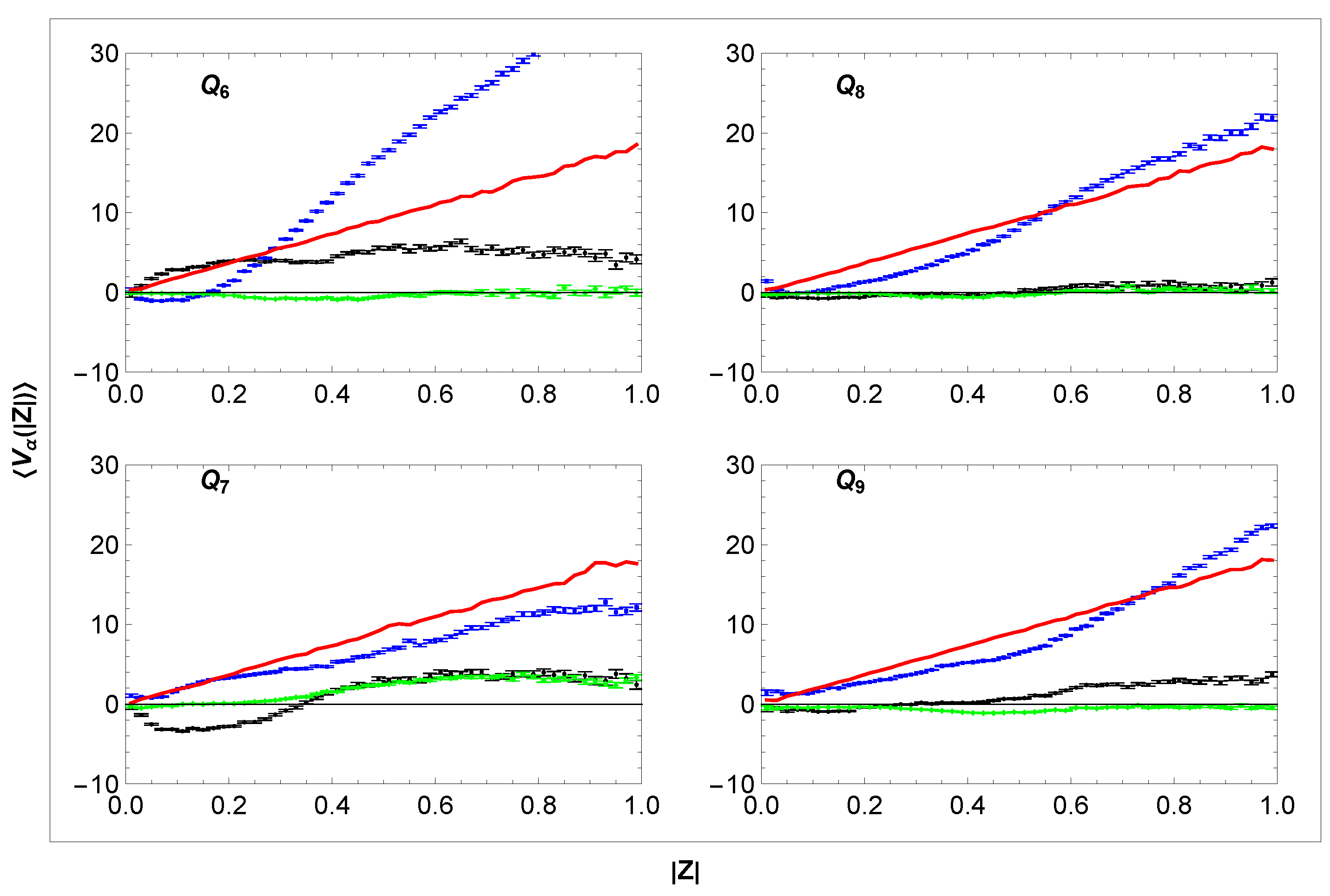
In Figure 15, we show the velocity curves in the sectors outside the galactic plane as functions of distance . Local fluctuations of and in all analysed sectors do not exceed 5 km/s. On the other hand, a clear increase in is observed in all sectors. The corresponding simulation, represented by a linear curve controlled by Equation (20), which is common to all sectors, is clearly only an approximation. The differences between the measured data and the simulation vary across different sectors. For and , the simulations yield a net zero (not shown in the figure).
Figure 15.
Dependence (blue, simulation red) (green), and (black) on distance from the galactic plane in sectors Qα. Units: V [km/s], Z [kpc].
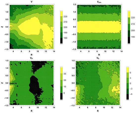
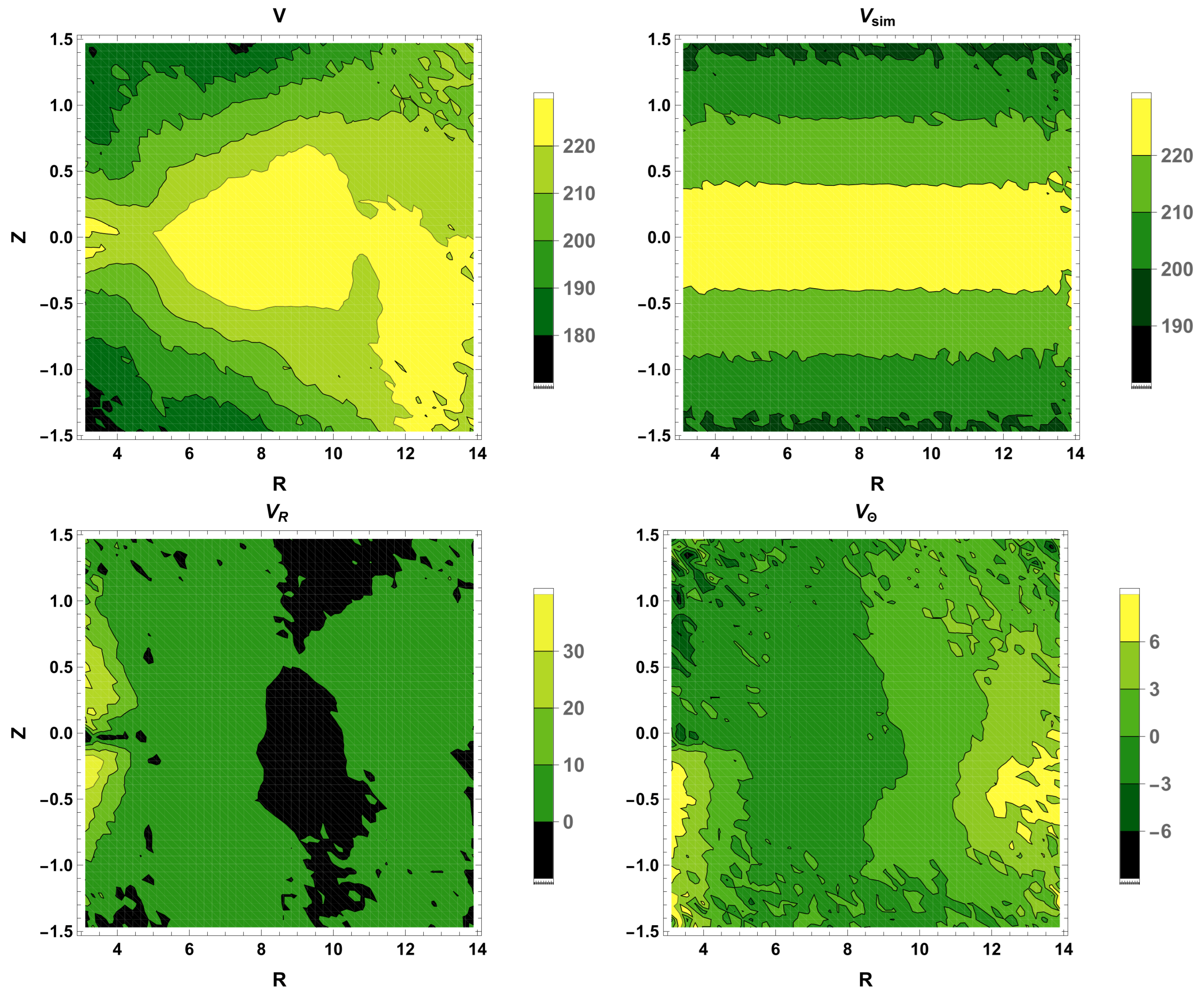
Diagrams of the rotation velocity , radial velocity , polar velocity , and simulated rotation velocity obtained from all sectors are shown in Figure 16.
Figure 16.
The diagrams. Top: rotation velocity and simulated rotation velocity . Bottom: radial velocity and polar velocity . Units: V [km/s], [kpc].
The plots provide additional information about the kinematics of the MW in the depicted region. Consistent with the left panel of Figure 13, we again observe that the decrease in rotation velocity in the region kpc is accompanied by a centrifugal component in . We also observe a slight asymmetry in at smaller R. For , is dominant; conversely, for , dominates.
The rotation velocity decreases as increases. This decrease is more pronounced for smaller (sector ) and less pronounced for larger (sector ). This pattern is more complex than the pattern from the simulation Vsim(Rc,Z), which assumes a constant slope throughout the entire region (see Equation (20)).
6. Discussion and Conclusions
Using a subset of the DR3 data from the Gaia space observatory, which includes information on radial velocities, we studied the 3D kinematics of the MW. This builds on our earlier 2D analysis, which relied on high-statistics data on stars without defined radial velocities. Although the two approaches differ in both method and input dataset, they yield identical or very close results, for example, concerning the Sun’s local velocity and the mean rotation velocity at radius .
As for , the component perpendicular to the galactic disk plane remains completely unchanged. The velocity also remains unchanged. It is important to emphasise that both velocities and are obtained completely independently of each other by analysing the stellar velocities in sectors . For measurements, sectors and are optimal, with a total sample of 3,737,755 stars. It follows from Equations (27)–(29) and Table 3 that the Sun’s total velocity km/s (that is, it does not contain the parameter ). Our result is consistent with a very reliable estimate of km/s based on the longitudinal speed of the radio source Sgr A*[48] and with the total velocity of km/s obtained in [43]. Very good agreement with other measurements also holds for the average rotation velocity km/s and the Sun’s local velocities , as shown in our previous 2D analysis.
Important results are the curves and and the corresponding diagrams in Figure 13, Figure 15, and Figure 16. In the region kpc in the figures, we observe fluctuations of local kinematic substructures in the range up to 10 km/s. The behaviour of the curves in the region kpc may be related to the proximity of the galactic bar.
Our velocity curve in Figure 14 agrees very well (in the overlap region) with the velocity curves presented in recent studies [7,15,20,21], which were also obtained using the Gaia DR3 catalogue. Small differences may be due to the parameters for the selection of stars, including the shape of the selection region.
As can be seen in Figure 15 and Figure 16, the average rotation velocity of stars slightly decreases with increasing . Therefore, to determine the curves and accurately, the selection region around the galactic plane should be as narrow as possible. That is why we used a very narrow range to generate the curve. This strict cut affects the curve particularly in the region kpc.
The decrease in rotation velocity with increasing has also been described in [20,44]. This effect is consistent with the Besançon Galaxy model [49], which provides a prediction for the region . This prediction agrees well with our curves in the sectors and of Figure 15, where . Asymmetric drift and a mixed population of thin and thick disks most likely contribute to the negative vertical gradient.
A useful tool in the analysis of stellar velocities is a simple MC simulation model described in Section 4. The simulation corresponds to an averaged axisymmetric approximation of the MW, so it may be useful in validating axisymmetric dynamical models or determining the scale of local kinematical substructures out of axial symmetry. The simulation model describes the distribution of velocities , and in the region kpc. Some discrepancy between the simulated and the data in sectors and was mentioned in the previous section (Figure 7, Figure 9, Figure 10, Figure 12, and Figure 15). The simulations play an important role in determining the parameter in Figure 5. In the relevant sectors and , the agreement with the simulation is perfect in the region kpc. In these sectors, we also observe very good agreement between the measured data and the simulation for all velocity distributions, as can be seen in Figure 7, Figure 8 and Figure 9, sector . In other sectors where simulations yield poorer results, introducing additional free parameters into the MC generator would improve the fit to the data.
The goal was to present a methodology for the kinematic analysis of the MW. We have shown that our approach makes it possible—using only two external parameters ( and ) taken from other studies—to derive, with reasonable accuracy, valuable results that are fully consistent with the findings of other studies. It should be noted that the parameter , which characterises asymmetric drift, is a quantity derived from Jeans modelling [50], which necessarily assumes an axially symmetric gravitational potential. It would certainly be interesting to attempt to calculate the function for subsamples of different ages within the global and, presumably, time-dependent gravitational potential. It is clear, however, that solving such a problem would require further independent research.
In conclusion, we believe that the proposed methods for calculating the local velocity of the Sun, the average rotation velocity , the velocity curve , and, more generally, the velocity maps , and represent a useful contribution to the analysis, description, and understanding of the global kinematics of the MW. The MC simulation model proved to be an effective tool in our study.
Author Contributions
Conceptualization, P.Z.; Methodology, P.Z.; Software, P.Z. and K.P.; Validation, P.Z.; Formal analysis, P.Z. and K.P.; Investigation, P.Z.; Data curation, K.P.; Writing—original draft, P.Z.; Writing—review and editing, K.P.; Supervision, P.Z. All authors have read and agreed to the published version of the manuscript.
Funding
This research received no external funding.
Data Availability Statement
The data underlying this article were accessed from the European Space Agency (ESA) mission Gaia (https://www.cosmos.esa.int/gaia (accessed on 29 May 2025)) and from publicly available cited references. The derived data generated in this research will be shared on reasonable request to the corresponding author.
Acknowledgments
This work made use of data from the European Space Agency (ESA) mission Gaia (https://www.cosmos.esa.int/gaia (accessed on 8 October 2026)), processed by the Gaia Data Processing and Analysis Consortium (DPAC, https://www.cosmos.esa.int/web/gaia/dpac/consortium (accessed on 8 October 2026)). Funding for the DPAC was provided by national institutions, in particular the institutions participating in the Gaia Multilateral Agreement. We would also like to express our sincere gratitude to the anonymous reviewers for their thorough evaluation of the manuscript and their valuable and constructive suggestions, which have helped us improve its quality.
Conflicts of Interest
The authors declare no conflicts of interest.
Appendix A. Reference Frames
The relation between galactic and Galactocentric reference frames is illustrated in Figure A1.
Figure A1.
Galactic (green) and Galactocentric (red) reference frames.
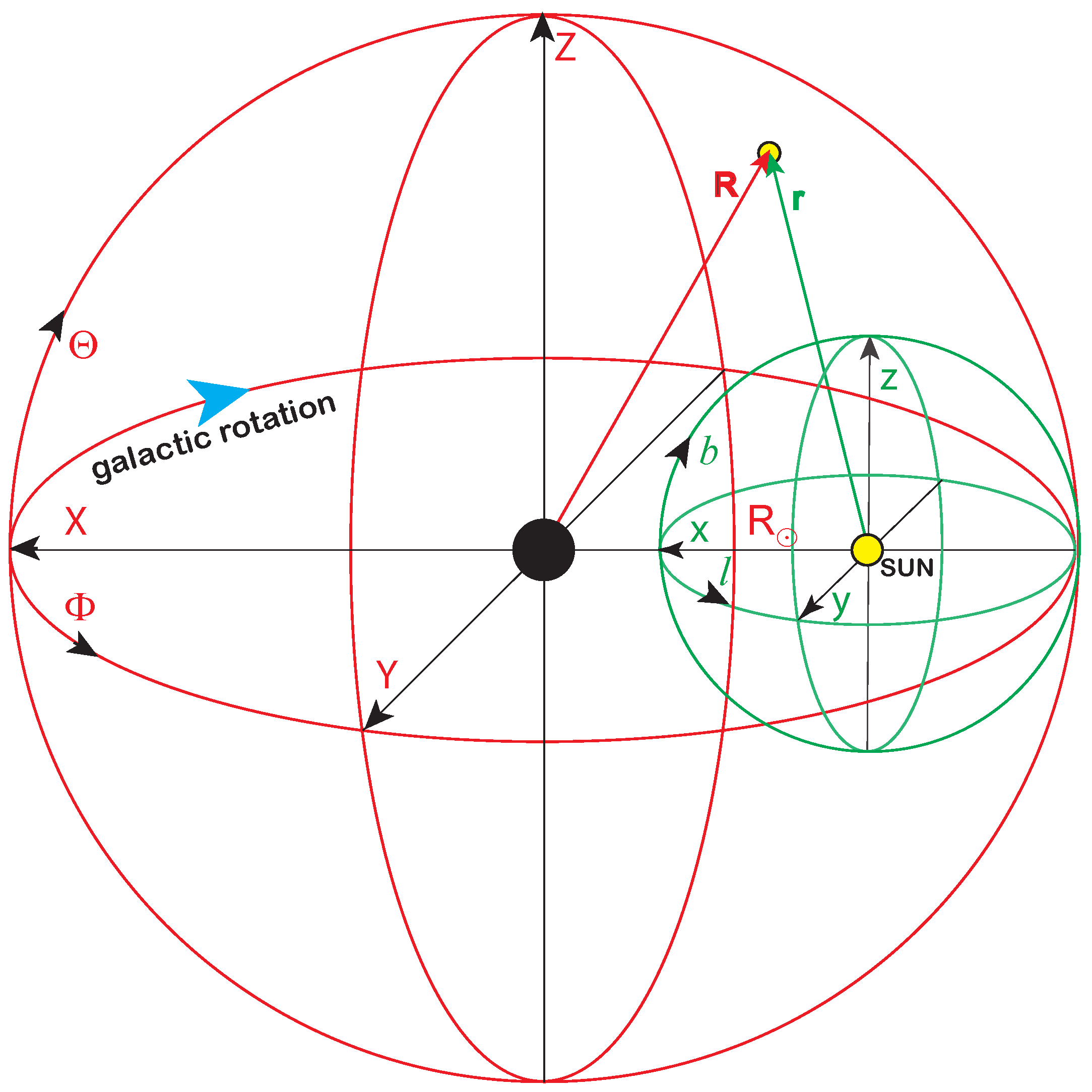
The axes are defined as
The axis therefore points towards the centre of the Galaxy, and the axis indicates the direction of the MW’s rotation. The corresponding coordinates are related as
The radius represents the distance of the Sun from the galactic centre. The small parameter kpc [51], defining the position of the Sun above the galactic plane, is neglected in our analysis, as justified in [39]. Then, the transformation between the spherical coordinates of both frames is defined by the equations
and inversely, :
where are defined by (A1). The spherical coordinates are simply related to the cylindrical coordinates :
In our analysis, we need vectors forming the local orthonormal bases in both reference frames:
where the vectors and define directions of increasing coordinates . For example, is the direction of the MW rotation at any point.
References
- Vallenari, A.; Brown, A.G.; Prusti, T.; De Bruijne, J.H.; Arenou, F.; Babusiaux, C.; Biermann, M.; Creevey, O.L.; Ducourant, C.; Evans, D.W.; et al. Gaia Data Release 3: Summary of the content and survey properties. Astron. Astrophys. 2023, 674, A1. [Google Scholar] [CrossRef] [Scilit]
- Zavada, P.; Píška, K. Statistical Analysis of Binary Stars from the Gaia Catalog Data Release 2. Astron. J. 2020, 159, 33. [Google Scholar] [CrossRef] [Scilit]
- Zavada, P.; Píška, K. Catalog of Wide Binary, Trinary and Quaternary Candidates from the Gaia Data Release 2. Astron. J. 2022, 163, 33. [Google Scholar] [CrossRef] [Scilit]
- Antoja, T.; Roca-Fàbrega, S.; De Bruijne, J.; Prusti, T. Kinematics of symmetric Galactic longitudes to probe the spiral arms of the Milky Way with Gaia. Astron. Astrophys. 2016, 589, A13. [Google Scholar] [CrossRef] [Scilit]
- Antoja, T.; Helmi, A.; Romero-Gḿez, M.; Katz, D.; Babusiaux, C.; Drimmel, R.; Evans, D.W.; Figueras, F.; Poggio, E.; Reylé, C.; et al. A dynamically young and perturbed Milky Way disk. Nature 2018, 561, 360. [Google Scholar] [CrossRef] [Scilit] [PubMed]
- Ablimit, I.; Zhao, G. The Milky Way’s Circular Velocity Curve and Its Constraint on the Galactic Mass with RR Lyrae Stars. Astrophys. J. 2017, 846, 10. [Google Scholar] [CrossRef] [Scilit]
- Beordo, W.; Crosta, M.; Lattanzi, M.G.; Re Fiorentin, P.; Spagna, A. Geometry-driven and dark-matter-sustained Milky Way rotation curves with Gaia DR3. Mon. Not. R. Astron. Soc. 2024, 529, 4681. [Google Scholar] [CrossRef] [Scilit]
- Bhattacharjee, P.; Chaudhury, S.; Kundu, S. Rotation Curve of the Milky Way out to 200 kpc. Astrophys. J. 2014, 785, 63. [Google Scholar] [CrossRef] [Scilit]
- Burch, B.; Cowsik, R. Properties of Galactic Dark Matter: Constraints from Astronomical Observations. Astrophys. J. 2013, 779, 35. [Google Scholar] [CrossRef] [Scilit]
- Chrobáková, Ž.; López-Corredoira, M.; Sylos Labini, F.; Wang, H.F.; Nagy, R. Gaia-DR2 extended kinematical maps: III. Rotation curves analysis, dark matter, and MOND tests. Astron. Astrophys. 2020, 642, A95. [Google Scholar] [CrossRef] [Scilit]
- Eilers, A.C.; Hogg, D.W.; Rix, H.W.; Ness, M.K. The Circular Velocity Curve of the Milky Way from 5 to 25 kpc. Astrophys. J. 2019, 871, 120. [Google Scholar] [CrossRef] [Scilit]
- Huang, Y.; Liu, X.W.; Yuan, H.B.; Xiang, M.S.; Zhang, H.W.; Chen, B.Q.; Ren, J.J.; Wang, C.; Zhang, Y.; Hou, Y.H.; et al. The Milky Way’s rotation curve out to 100 kpc and its constraint on the Galactic mass. Mon. Not. R. Astron. Soc. 2016, 463, 2623. [Google Scholar] [CrossRef] [Scilit]
- Jiao, Y.; Hammer, F.; Wang, J.L.; Yang, Y.B. Which Milky Way masses are consistent with the slightly declining 5–25 kpc rotation curve? Astron. Astrophys. 2021, 654, A25. [Google Scholar] [CrossRef] [Scilit]
- Mróz, P.; Udalski, A.; Skowron, D.M.; Skowron, J.; Soszyłski, I.; Pietrukowicz, P.; Szymałski, M.K.; Poleski, R.; Kozłowski, S.; Ulaczyk, K. Rotation Curve of the Milky Way from Classical Cepheids. Astrophys. J. Lett. 2019, 870, 10. [Google Scholar] [CrossRef] [Scilit]
- Ou, X.; Eilers, A.-C.; Necib, L.; Frebel, A. The dark matter profile of the Milky Way inferred from its circular velocity curve. Mon. Not. R. Astron. Soc. 2024, 528, 693. [Google Scholar] [CrossRef] [Scilit]
- Reid, M.J.; Menten, K.M.; Brunthaler, A.; Zheng, X.W.; Dame, T.M.; Xu, Y.; Wu, Y.; Zhang, B.; Sanna, A.; Sato, M.; et al. Trigonometric Parallaxes of High Mass Star Forming Regions. Astrophys. J. 2014, 783, 130. [Google Scholar] [CrossRef] [Scilit]
- Wegg, C.; Gerhard, O.; Bieth, M. The gravitational force field of the Galaxy measured from the kinematics of RR Lyrae in Gaia. Mon. Not. R. Astron. Soc. 2019, 485, 3296. [Google Scholar] [CrossRef] [Scilit]
- Sofue, Y. Rotation Curve of the Milky Way and the Dark Matter Density. Galaxies 2020, 8, 37. [Google Scholar] [CrossRef] [Scilit]
- Sylos Labini, F.; Chrobáková, Ž.; Capuzzo-Dolcetta, R.; López-Corredoira, M. Mass Models of the Milky Way and Estimation of Its Mass from the Gaia DR3 Data Set. Astrophys. J. 2023, 945, 3. [Google Scholar] [CrossRef] [Scilit]
- Wang, H.F.; Chrobáková, Ž.; López-Corredoira, M.; Sylos Labini, F. Mapping the Milky Way Disk with Gaia DR3: 3D Extended Kinematic Maps and Rotation Curve to ≈30 kpc. Astrophys. J. 2023, 942, 12. [Google Scholar] [CrossRef] [Scilit]
- Zhou, Y.; Li, X.; Huang, Y.; Zhang, H. The Circular Velocity Curve of the Milky Way from 5–25 kpc Using Luminous Red Giant Branch Stars. Astrophys. J. 2023, 946, 73. [Google Scholar] [CrossRef] [Scilit]
- Jiao, Y.; Hammer, F.; Wang, H.; Wang, J.; Amram, P.; Chemin, L.; Yang, Y. Detection of the Keplerian decline in the Milky Way rotation curve. Astron. Astrophys. 2023, 678, A208. [Google Scholar] [CrossRef] [Scilit]
- Drimmel, R. et al. [Gaia Collaboration] Gaia Data Release 3: Mapping the asymmetric disc of the Milky Way. Astron. Astrophys. 2023, 674, A37. [Google Scholar] [CrossRef] [Scilit]
- Katz, D.; Antoja, T.; Romero-Gómez, M.; Drimmel, R.; Reylé, C.; Seabroke, G.M.; Soubiran, C.; Babusiaux, C.; Di Matteo, P.; Figueras, F.; et al. Gaia Data Release 2: Mapping the Milky Way disc kinematics. Astron. Astrophys. 2018, 616, A11. [Google Scholar] [CrossRef] [Scilit]
- Kawata, D.; Baba, J.; Ciucă, I.; Cropper, M.; Grand, R.J.; Hunt, J.A.; Seabroke, G. Radial distribution of stellar motions in Gaia DR2. MNRAS Lett. 2018, 479, 108. [Google Scholar] [CrossRef] [Scilit]
- Kawata, D.; Bovy, J.; Matsunaga, N.; Baba, J. Galactic rotation from Cepheids with Gaia DR2 and effects of non-axisymmetry. Mon. Not. R. Astron. Soc. 2019, 482, 40. [Google Scholar] [CrossRef] [Scilit]
- Kushniruk, I.; Schirmer, T.; Bensby, T. Kinematic structures of the solar neighbourhood revealed by Gaia DR1/TGAS and RAVE. Astron. Astrophys. 2017, 608, A73. [Google Scholar] [CrossRef] [Scilit]
- López-Corredoira, M.; Sylos Labini, F. Gaia-DR2 extended kinematical maps. Astron. Astrophys. 2019, 621, A48. [Google Scholar] [CrossRef] [Scilit]
- Ramos, P.; Antoja, T.; Figueras, F. Riding the kinematic waves in the Milky Way disk with Gaia. Astron. Astrophys. 2018, 619, A72. [Google Scholar] [CrossRef] [Scilit]
- Tian, H.J.; Liu, C.; Wan, J.C.; Wang, Y.G.; Wang, Q.; Deng, L.C.; Cao, Z.H.; Hou, Y.H.; Wang, Y.F.; Wu, Y.; et al. Peculiar in-plane velocities in the outer disc of the Milky Way. Res. Astron. Astrophys. 2017, 17, 114. [Google Scholar] [CrossRef] [Scilit]
- Wang, H.F.; López-Corredoira, M.; Huang, Y.; Carlin, J.L.; Chen, B.Q.; Wang, C.; Chang, J.; Zhang, H.W.; Xiang, M.S.; Yuan, H.B.; et al. Mapping the Galactic disc with the LAMOST and Gaia red clump sample: II. 3D asymmetrical kinematics of mono-age populations in the disc between 6–14 kpc. Mon. Not. R. Astron. Soc. 2020, 491, 2104. [Google Scholar] [CrossRef] [Scilit]
- Bland-Hawthorn, J.; Gerhard, O. The Galaxy in Context: Structural, Kinematic, and Integrated Properties. Annu. Rev. Astron. Astrophys. 2016, 54, 529. [Google Scholar] [CrossRef] [Scilit]
- Navarro, J.F.; Frenk, C.S.; White, S.D.M. A Universal Density Profile from Hierarchical Clustering. Astrophys. J. 1997, 490, 493. [Google Scholar] [CrossRef] [Scilit] [PubMed]
- Stephanovich, V.A.; Godłowski, W. The Distribution of Galaxies’ Gravitational Field Stemming from their Tidal Interaction. Astrophys. J. 2015, 810, 167. [Google Scholar] [CrossRef] [Scilit]
- Codis, S.; Jindal, A.; Chisari, N.E.; Vibert, D.; Dubois, Y.; Pichon, C.; Devriendt, J. Galaxy orientation with the cosmic web across cosmic time. Mon. Not. R. Astron. Soc. 2018, 481, 4753. [Google Scholar] [CrossRef] [Scilit]
- Okabe, T.; Nishimichi, T.; Oguri, M.; Peirani, S.; Kitayama, T.; Sasaki, S.; Suto, Y. Projected alignment of non-sphericities of stellar, gas, and dark matter distributions in galaxy clusters: Analysis of the Horizon-AGN simulation. Mon. Not. R. Astron. Soc. 2018, 478, 1141. [Google Scholar] [CrossRef] [Scilit]
- Stephanovich, V.A.; Godłowski, W.; Biernacka, M. The Influence of Dark Matter Halos on Galaxies’ Orbital Momenta Alignment. Res. Astron. Astrophys. 2025, 25, 115002. [Google Scholar] [CrossRef] [Scilit]
- Katz, D. et al. [Gaia Collaboration] Gaia Data Release 3: Properties and validation of the radial velocities. Astron. Astrophys. 2023, 674, A5. [Google Scholar] [CrossRef] [Scilit]
- Zavada, P.; Píška, K. Kinematics of the Milky Way from the Statistical Analysis of the Gaia Data Release 3. Galaxies 2025, 13, 10. [Google Scholar] [CrossRef] [Scilit]
- Gaia Data Processing and Analysis Consortium 2023, Gaia Data Release 3, Documentation Release 1.3. Available online: https://gea.esac.esa.int/archive/documentation/GDR3/ (accessed on 8 October 2026).
- Ramos, P. gaiadr3-zeropoint 0.1.0 (Python3 package), ver.0.1.0, 2025. Available online: https://pypi.org/project/gaiadr3-zeropoint/ (accessed on 8 October 2026).
- Lindegren, L.; Bastian, U.; Biermann, M.; Bombrun, A.; de Torres, A.; Gerlach, E.; Geyer, R.; Hernandez, J.; Hilger, T.; Hobbs, D.; et al. Gaia Early Data Release 3: Parallax bias versus magnitude, colour, and position. Astron. Astrophys. 2021, 649, A4. [Google Scholar] [CrossRef] [Scilit]
- Abuter, R.; Amorim, A.; Bauböck, M.; Berger, J.P.; Bonnet, H.; Brandner, W.; Clénet, Y.; Du Foresto, V.C.; De Zeeuw, P.T.; Dexter, J.; et al. A geometric distance measurement to the Galactic center black hole with 0.3% uncertainty. Astron. Astrophys. 2019, 625, L10. [Google Scholar] [CrossRef] [Scilit]
- Anguiano, B.; Majewski, S.R.; Hayes, C.R.; Prieto, C.A.; Cheng, X.; Bidin, C.M.; Beaton, R.L.; Beers, T.C.; Minniti, D. The Stellar Velocity Distribution Function in the Milky Way Galaxy. Astron. J. 2020, 160, 43. [Google Scholar] [CrossRef] [Scilit]
- Vieira, K.; Carraro, G.; Korchagin, V.; Lutsenko, A.; Girard, T.M.; van Altena, W. Milky Way Thin and Thick Disk Kinematics with Gaia EDR3 and RAVE DR5. Astrophys. J. 2022, 932, 28. [Google Scholar] [CrossRef] [Scilit]
- Li, X.; Yang, P.; Wang, H.F.; Li, Q.; Luo, Y.P.; Luo, Z.Q.; Wang, G.Y. Asymmetric Drift Map of the Milky Way disk Populations between 8–16 kpc with LAMOST and Gaia datasets. arXiv 2023, arXiv:2310.01311. [Google Scholar]
- Schönrich, R.; Binney, J.; Dehnen, W. Local kinematics and the local standard of rest. Mon. Not. R. Astron. Soc. 2010, 403, 1829. [Google Scholar] [CrossRef] [Scilit]
- Reid, M.J.; Brunthaler, A. The Proper Motion of Sagittarius A★.III. The Case for a Supermassive Black Hole. Astrophys. J. 2020, 892, 39. [Google Scholar] [CrossRef] [Scilit]
- Bienaymé, O.; Leca, J.; Robin, A.C. A new dynamically self-consistent version of the Besançon Galaxy model. Astron. Astrophys. 2018, 620, A103. [Google Scholar] [CrossRef] [Scilit]
- Jeans, J.H. On the theory of star-streaming and the structure of the universe. Mon. Not. R. Astron. Soc. 1915, 76, 70. [Google Scholar] [CrossRef] [Scilit]
- Bennet, M.; Bovy, J. Vertical waves in the solar neighbourhood in Gaia DR2. Mon. Not. R. Astron. Soc. 2019, 482, 1417. [Google Scholar] [CrossRef] [Scilit]

Disclaimer/Publisher’s Note: The statements, opinions and data contained in all publications are solely those of the individual author(s) and contributor(s) and not of MDPI and/or the editor(s). MDPI and/or the editor(s) disclaim responsibility for any injury to people or property resulting from any ideas, methods, instructions or products referred to in the content. |
© 2026 by the authors. Licensee MDPI, Basel, Switzerland. This article is an open access article distributed under the terms and conditions of the Creative Commons Attribution (CC BY) license.