On Family-Separated Seesaw Relations: Exact Reconstruction and Corrections

Abstract

We examine the family-separated seesaw (FSS) ansatz proposed in arXiv:2605.27049v2. Combining its paired cancellations with exact partial unitarity fixes the light and heavy mixing blocks in terms of one unitary matrix and the paired mass ratios. We classify their unitary completions and reconstruct the Dirac and singlet Majorana mass matrices, distinguishing the physical heavy masses from the singlet mass parameters. This identifies FSS as an exact realization of form dominance whose conventional one-loop leptogenesis cancellation is already established. The particular sum of lepton-number-violating invariants entering the proposed decay asymmetry therefore vanishes; individual CP invariants need not vanish. We also correct the heavy-mass reconstruction formulas and quantify their errors for both light-mass orderings. These formulas are conditional algebraic relations, not independent predictions of the heavy spectrum. Numerical mass–mixing illustrations, explicit chiral projections for double-beta decay, and a leading-logarithmic estimate of radiative misalignment clarify the physical reach and limitations. The contribution is an exact consistency analysis and correction of specific proposed consequences rather than a new mass-generation mechanism or a general prohibition of leptogenesis.

1. Introduction

The canonical type-I seesaw generates Majorana neutrino masses by adding gauge-singlet fermions to the Standard Model [1,2,3,4,5]. With three singlets, let U and R denote the upper light and heavy blocks of the unitary $6\times 6$ neutral-lepton mixing matrix. Exact diagonalization implies

$$U{D}_{\nu }{U}^T+R{D}_N{R}^T=0,U{U}^{†}+R{R}^{†}=\mathbf{1},D_{\nu }=\mathrm{diag}\left(m_i\right),D_N=\mathrm{diag}\left(M_i\right).$$

(1)

Here $m_i\ge 0$ and $M_i>0$ are Takagi masses of the complete broken-phase mass matrix [6,7,8]. The family-separated seesaw (FSS) ansatz of Ref. [9] imposes the stronger, paired conditions

$$m_i{U}_{\alpha i}{U}_{\beta i}+M_i{R}_{\alpha i}{R}_{\beta i}=0(i=1,2,3;\alpha ,\beta =e,\mu ,\tau ).$$

(2)

Throughout, Ref. [9] means version 2 of arXiv:2605.27049, and a definite light–heavy pairing is fixed. “Exact” means an identity of the renormalized tree-level mass matrix at a common scale, not an all-loop or thermal statement.

The physical question is whether this restrictive ansatz supports the standard decay source used in early-Universe leptogenesis. Orthogonal Yukawa columns and their vanishing conventional flavored and unflavored decay asymmetries are established properties of form dominance [10,11,12]. Our purpose is to apply that knowledge consistently to the exact FSS relations and to correct two specific consequences proposed in Ref. [9]: the interpretation of its decay-asymmetry expression and its heavy-mass reconstruction formulas. Version 2 already distinguishes ordinary-oscillation Jarlskog invariants from lepton-number-violating (LNV) invariants. Our criticism concerns the particular flavor sum of the latter in Equation (12), not a purported identification with the ordinary-oscillation invariant.

It is useful to separate three levels of results. First, the leptogenesis cancellation for form dominance is known. Second, paired column proportionality, orthogonality, and the relevant invariant cancellations are already implicit in FSS together with partial unitarity. Third, the contribution developed here is their complete constructive realization: all unitary completions of the fixed upper blocks, the exact conversion between physical masses and singlet parameters, and an explicit correction and numerical comparison of the proposed mass formulas. The underlying two-state seesaw physics is familiar; its assembly into a general completion establishes that no algebraic higher-order correction in light–heavy mixing restores the specified decay source while exact FSS holds. It does not introduce a separate mass-generation mechanism.

Section 2 gives the reconstruction and its precise relation to form dominance. Section 3 states the decay cancellation compactly. Section 4 corrects and tests the mass formulas. Section 5 and Section 6 discuss measurable scales, chiral amplitudes, symmetry motivation, and a controlled estimate of radiative breaking.

2. Exact Reconstruction and Its Relation to Form Dominance

2.1. Upper Blocks and Completeness

Let $u_i$ and ${\rho }_i$ be the ith columns of U and R. For $m_i>0$, the equality $m_i{u}_i{u}_i^T=-M_i{\rho }_i{\rho }_i^T$ forces the two nonzero rank-one images to coincide. Thus ${\rho }_i={\lambda }_i{u}_i$ and ${\lambda }_i^2=-m_i/M_i$. If $m_i=0$, instead ${\rho }_i=0$. No entire pair $(u_i,{\rho }_i)$ can vanish: the two remaining paired contributions to $U{U}^{†}+R{R}^{†}$ each have rank at most one and cannot sum to ${\mathbf{1}}_3$. Hence, including the massless case,

$$R=UC,C=iE\mathrm{diag}\left(\sqrt{r_i}\right),r_i={\displaystyle \frac{m_i}{M_i}},E=\mathrm{diag}\left({\eta }_i\right),{\eta }_i=\pm 1.$$

(3)

The same sign applies to every flavor in one column; these signs are Majorana column conventions, not additional physical phases. Writing $D=\mathbf{1}+C{C}^{†}=\mathrm{diag}(1+r_i)$, partial unitarity reads $UD{U}^{†}=\mathbf{1}$. Therefore $V=U{D}^{1/2}$ is square and unitary, giving the general solution

$$U=V{C}_r,R=iVE{S}_r,C_r=\mathrm{diag}{\displaystyle \frac{1}{\sqrt{1+r_i}}},S_r=\mathrm{diag}\sqrt{{\displaystyle \frac{r_i}{1+r_i}}}.$$

(4)

In particular,

$$\begin{array}{cccccc}\hfill U^{†}U& =D^{-1},\hfill & \hfill R^{†}R& =\mathbf{1}-D^{-1},\hfill & \hfill U^{†}R& =iE\mathrm{diag}{\displaystyle \frac{\sqrt{r_i}}{1+r_i}}.\hfill \end{array}$$

(5)

Distinct columns are orthogonal, and $U^{†}U+R^{†}R=\mathbf{1}$. The latter is a special paired FSS identity, unlike the generic upper-row unitarity condition in Equation (1). Conversely, $C{D}_N{C}^T=-D_{\nu }$ verifies the seesaw relation directly.

For any unitary sterile-basis matrix W, a completion is

$$\mathcal{U}=\left(\begin{array}{cc}V{C}_r& iVE{S}_r\\ iWE{S}_r& W{C}_r\end{array}\right),\mathcal{U}{\mathcal{U}}^{†}={\mathbf{1}}_6.$$

(6)

This is the most general completion of the fixed upper blocks: the lower three rows form an orthonormal basis of their orthogonal complement, and two such bases differ precisely by left multiplication by W. With the convention

$$\mathcal{M}=\left(\begin{array}{cc}0& M_D\\ M_D^T& M_R\end{array}\right)=\mathcal{U}\mathrm{diag}(D_{\nu },D_N){\mathcal{U}}^T,$$

(7)

one obtains

$$M_D=iVE{\left(D_{\nu }{D}_N\right)}^{1/2}{W}^T,M_R=W(D_N-D_{\nu })W^T.$$

(8)

These are identities of chiral mass matrices. They do not replace spinor amplitudes or assume that physical processes are helicity-independent.

2.2. Masses, Yukawa Couplings, and the Two-State Interpretation

Choose $W=\mathbf{1}$. In the canonical domain $M_i>m_i$, the positive singlet Takagi masses are

$${\widehat{M}}_i=M_i-m_i,Y_{\nu }={\displaystyle \frac{i}{v}}VE{\left(D_{\nu }{D}_N\right)}^{1/2},H\equiv Y_{\nu }^{†}{Y}_{\nu }={\displaystyle \frac{D_{\nu }{D}_N}{v^2}},v=⟨{\varphi }^0⟩\simeq 174\mathrm{GeV}.$$

(9)

We denote the singlet mass eigenfields by ${\mathcal{N}}_i$ to distinguish them from the exact broken-phase heavy eigenstates $N_i$. The usual unbroken-phase decay description uses $({\mathcal{N}}_i,{\widehat{M}}_i,Y_{\nu })$; its thermal application also requires an electroweak-symmetric decay epoch, which $M_i>m_i$ alone does not ensure. The exact conversion is

$$R_{\alpha i}={\displaystyle \frac{v{\left(Y_{\nu }\right)}_{\alpha i}}{\sqrt{M_i(M_i+m_i)}}},y_i^2\equiv H_{ii}={\displaystyle \frac{m_i{M}_i}{v^2}}.$$

(10)

An active congruence by $V^{\ast }$ and a permutation into paired order reduce the neutrino mass matrix to

$${\displaystyle \underset{i=1}{\overset{3}{⨁}}}\left(\begin{array}{cc}0& i{\eta }_i\sqrt{m_i{M}_i}\\ i{\eta }_i\sqrt{m_i{M}_i}& M_i-m_i\end{array}\right).$$

(11)

The familiar two-state relations $|M_{D,i}{|}^2=m_i{M}_i$ and $M_{R,i}=M_i-m_i$ are thus recovered. The useful step is proving that every completion of the original upper-block ansatz has this structure up to a sterile basis rather than assuming it initially. Only the neutrino mass sector decouples in this basis; V still fixes the charged-current flavor directions relative to charged leptons.

The link to form dominance can be made exact without conflating mass definitions. The tree-level zero-momentum Schur complement is

$$m_{\mathrm{eff}}=-M_D{M}_R^{-1}{M}_D^T=V{\tilde{D}}_{\nu }{V}^T,{\left({\tilde{D}}_{\nu }\right)}_{ii}={\displaystyle \frac{m_i{M}_i}{M_i-m_i}}.$$

(12)

Its Takagi singular values are those of the dimension-five mass matrix, not the exact physical light masses; finite-mixing kinetic and higher-dimensional effects distinguish them. In the Casas–Ibarra representation $M_D=iV{\tilde{D}}_{\nu }^{1/2}O{\widehat{D}}_N^{1/2}$, ${\widehat{D}}_N=\mathrm{diag}\left({\widehat{M}}_i\right)$, one has $O=E$ exactly [10,11,13]. The usual identification using the physical light masses instead is a seesaw-limit statement. Conversely, mutually orthogonal Dirac columns in a positive diagonal singlet basis reduce to Equation (11) after exact diagonalization. Thus orthogonal ultraviolet form-dominant textures can already realize exact FSS.

For $r_i\ll 1$, $U_i/V_i=1-r_i/2+O\left(r_i^2\right)$ and ${\widehat{M}}_i/M_i=1-r_i$. At $m_i=0.05$ eV and $M_i=1$ TeV, $r_i=5\times {10}^{-14}$. Exactness supplies consistency and completeness, not a sizable correction to ordinary high-scale phenomenology.

2.3. Domains and Parameter Freedom

For $m_i=0$ the paired R and Yukawa columns vanish; its light column remains nonzero. Formal continuation to $M_i<m_i$ gives a signed $M_i-m_i$ whose physical singlet Takagi value is $|M_i-m_i|$ after rephasing. At equality the singlet mass vanishes. Neither continuation has the conventional heavy-singlet interpretation used below. Degenerate nonzero Takagi masses allow real orthogonal rotations within their subspaces; a massless subspace has unitary freedom. Pairwise statements require a specified basis there. Degeneracies of $M_i$ and ${\widehat{M}}_i$ are distinct: in a degenerate singlet subspace an orthogonal rotation may make H nondiagonal, although Equation (9) supplies a simultaneous diagonal basis.

For a fixed pairing and generic nonzero, nondegenerate spectra, the restricted FSS model has twelve continuous neutrino-sector parameters: six masses, three angles, and three phases in V after charged-lepton rephasings. The ratios $r_i$ are already fixed by the masses, W is sterile basis freedom, and ${\eta }_i$ are sign conventions. A massless light neutrino removes one Majorana phase. This is not the parameter count of a general type-I seesaw. Accordingly, angles and phases in a general $6\times 6$ Euler parametrization cannot be varied independently after imposing FSS [8,14].

3. The Conventional Decay Source and the Invariant Cancellation

For nondegenerate positive ${\widehat{M}}_i$ sufficiently far from resonance, the standard vacuum one-loop decay asymmetry contains

$${ϵ}_i={\displaystyle \frac{1}{8\pi H_{ii}}}\sum _{k\ne i}\mathrm{Im}\left(H_{ik}^2\right)f\left(x_{ki}\right),x_{ki}={\widehat{M}}_k^2/{\widehat{M}}_i^2.$$

(13)

Its flavored counterpart contains $\mathrm{Im}\left[Y_{\alpha i}^{\ast }{Y}_{\alpha k}{H}_{ik}\right]$ and $\mathrm{Im}\left[Y_{\alpha i}^{\ast }{Y}_{\alpha k}{H}_{ki}\right]$, with the appropriate loop functions [15,16,17,18,19]. Equation (9) sets both off-diagonal factors to zero: ${ϵ}_i={ϵ}_{i\alpha }=0$ when $H_{ii}>0$. This is the known form-dominance result [11], now applicable without using the approximate conversion $R\simeq v{Y}_{\nu }{D}_N^{-1}$. If $m_i=0$, instead $H_{ii}=0$ and the Yukawa decay width vanishes; the normalized asymmetry is undefined, and this state supplies no decay source. Chiral Yukawa vertices and the usual spin sums are already included in these standard expressions; the cancellation is in their flavor coefficients.

The cancellation in the proposed expression can also be seen directly. Define the LNV invariants used in Ref. [9] by

$${\mathcal{V}}_{\alpha \beta }^{ik}=\mathrm{Im}\left(U_{\alpha i}{U}_{\beta i}{U}_{\alpha k}^{\ast }{U}_{\beta k}^{\ast }\right).\sum _{\alpha }{\mathcal{V}}_{\alpha \beta }^{ik}=\mathrm{Im}\left[U_{\beta i}{U}_{\beta k}^{\ast }\sum _{\alpha }{U}_{\alpha i}{U}_{\alpha k}^{\ast }\right]=0(i\ne k).$$

(14)

The fixed-$\beta$ identity immediately implies

$$\sum _{\alpha }{\mathcal{V}}_{\alpha \alpha }^{ik}+2\sum _{\alpha <\beta }{\mathcal{V}}_{\alpha \beta }^{ik}=0,\mathrm{Im}\left[{\left(R^{†}R\right)}_{ik}^2\right]=-r_i{r}_k\sum _{\alpha ,\beta }{\mathcal{V}}_{\alpha \beta }^{ik}=0.$$

(15)

We read the undefined superscript $jk$ in the second flavor sum of Equation (12) of Ref. [9] as $ik$, as required by its first sum and by this expansion. Individual LNV invariants, and independently ordinary-oscillation CP invariants, may remain nonzero. Their presence does not make the proposed sum nonzero.

This result concerns the common-scale, nonresonant one-loop source. Degenerate or sufficiently quasi-degenerate singlets require a separate basis-invariant coherent treatment [20,21]. Thermal, higher-loop, and helicity-resolved transport sources are not evaluated here; Ref. [22] provides one thermal example. These exclusions do not assert that such effects necessarily generate an asymmetry. Radiative breaking of the alignment is estimated in Section 6.

4. Corrected Conditional Heavy-Mass Relations

4.1. Definitions and Corrected Expressions

Use the Euler convention of Ref. [9], with $s_{ij}=\sin {\theta }_{ij}$, $c_{ij}=\cos {\theta }_{ij}$, $t_{ij}=\tan {\theta }_{ij}$ and $C_e=c_{14}{c}_{15}{c}_{16}$. Its electron row obeys

$$|U_{ei}{|}^2=C_e^2{w}_i,(w_1,w_2,w_3)=(c_{12}^2{c}_{13}^2,s_{12}^2{c}_{13}^2,s_{13}^2),\sum _i{w}_i=1.$$

(16)

Assuming heavy states are inaccessible in the beta spectrum, distinguish the unnormalized coefficient of Ref. [9] from the normalized unresolved-spectrum shape parameter [23]:

$$m_{\beta }^2=\sum _i{m}_i^2{\left|U_{ei}\right|}^2,m_{\beta ,\mathrm{norm}}^2={\displaystyle \frac{m_{\beta }^2}{C_e^2}}=\sum _i{w}_i{m}_i^2.$$

(17)

The second definition factors out the electron-row normalization. For available neutrino energy w with $w^2\gg m_i^2$, the spectral factor is ${\sum }_i{\left|U_{ei}\right|}^{2}w\sqrt{w^2-m_i^2}=C_e^2{w}^2-m_{\beta }^2/2+O(m_i^4/w^2)$. Thus Equation (17) is useful when normalization is fitted separately, not a substitute for a full endpoint analysis. Experimental masses must be matched to that convention; the Euler angles must likewise be inferred consistently if nonunitarity is appreciable.

With signed $\Delta m_{ij}^2=m_i^2-m_j^2$ and $\Delta m_{31}^2=\Delta m_{32}^2+\Delta m_{21}^2$, the standard weighted mass identities, independent of FSS, are simply

$$\begin{array}{cc}\hfill m_1^2& =m_{\beta ,\mathrm{norm}}^2-w_2\Delta m_{21}^2-w_3\Delta m_{31}^2,\hfill \\ \hfill m_2^2& =m_{\beta ,\mathrm{norm}}^2+w_1\Delta m_{21}^2-w_3\Delta m_{32}^2,\hfill \\ \hfill m_3^2& =m_{\beta ,\mathrm{norm}}^2+w_1\Delta m_{31}^2+w_2\Delta m_{32}^2.\hfill \end{array}$$

(18)

FSS adds $m_i|U_{ei}{|}^2=M_i{\left|R_{ei}\right|}^2$, where $|R_{e1}{|}^2=s_{14}^2{c}_{15}^2{c}_{16}^2$, $|R_{e2}{|}^2=s_{15}^2{c}_{16}^2$, and $|R_{e3}{|}^2=s_{16}^2$. Consequently $M_i=m_i{F}_i$, with

$$(F_1,F_2,F_3)=\left({\displaystyle \frac{w_1}{t_{14}^2}},{\displaystyle \frac{w_2{c}_{14}^2}{t_{15}^2}},{\displaystyle \frac{w_3{c}_{14}^2{c}_{15}^2}{t_{16}^2}}\right).$$

(19)

The corrected version of Equation (20) of Ref. [9] is therefore

$$\begin{array}{cc}\hfill M_1^2& =F_1^2[m_{\beta ,\mathrm{norm}}^2-w_2\Delta m_{21}^2-w_3\Delta m_{31}^2],\hfill \\ \hfill M_2^2& =F_2^2[m_{\beta ,\mathrm{norm}}^2+w_1\Delta m_{21}^2-w_3\Delta m_{32}^2],\hfill \\ \hfill M_3^2& =F_3^2[m_{\beta ,\mathrm{norm}}^2+w_1\Delta m_{31}^2+w_2\Delta m_{32}^2].\hfill \end{array}$$

(20)

Each bracket is precisely $m_i^2$. The denominators and canceled factors in Equation (19) must be nonzero. At a zero-angle, vanishing first-row element, massless limit, or singular Euler chart, use the undivided FSS relations instead: in particular, a vanishing Yukawa column does not determine its heavy mass by division.

4.2. Direct Comparison and Numerical Size

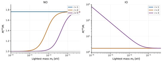
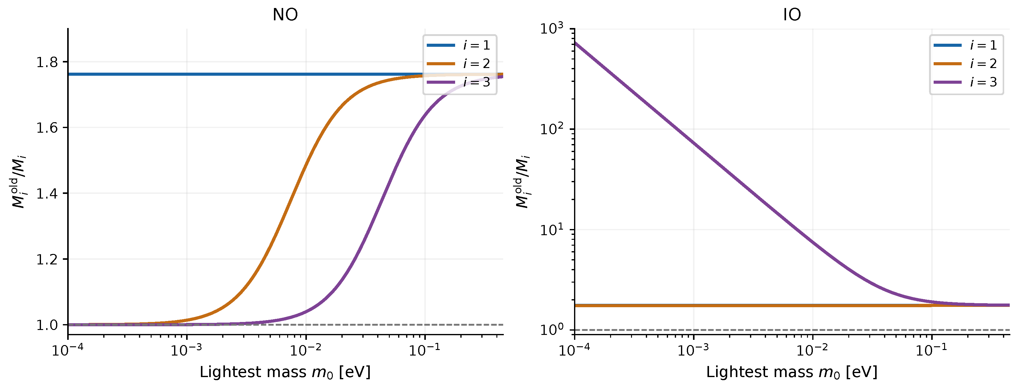
Let $q=w_2+w_3=1-w_1$, and use “old” only for the algebraic outputs of Equation (20) of Ref. [9] evaluated on the same inputs. Its three brackets divided by q are, respectively, $m_1^2/q$, $(m_2^2-w_1\Delta m_{21}^2)/q$, and $(m_3^2-w_1\Delta m_{31}^2)/q$. Thus

$${\displaystyle \frac{{\left(M_1^{\mathrm{old}}\right)}^2}{M_1^2}}={\displaystyle \frac{1}{q}},{\displaystyle \frac{{\left(M_2^{\mathrm{old}}\right)}^2}{M_2^2}}=1+{\displaystyle \frac{w_1{m}_1^2}{q{m}_2^2}},{\displaystyle \frac{{\left(M_3^{\mathrm{old}}\right)}^2}{M_3^2}}=1+{\displaystyle \frac{w_1{m}_1^2}{q{m}_3^2}}.$$

(21)

These ratios isolate both errors: the unnecessary common denominator and the missing $w_1\Delta m^2$ terms. They are independent of the active–heavy angles wherever the ratios are defined. For physical positive masses they overestimate, rather than underestimate, the corrected masses. In normal ordering (NO), the second and third ratios approach unity as $m_1\to 0$; in inverted ordering (IO), the third grows strongly as $m_3\to 0$. Exactly massless endpoints must still be treated with the undivided equations.

For reproducible illustrations we use rounded oscillation inputs $s_{12}^2=0.307$, $s_{13}^2=0.022$, $\Delta m_{21}^2=7.4\times {10}^{-5}{\mathrm{eV}}^2$ and $\Delta m_{31}^2=\pm 2.5\times {10}^{-3}{\mathrm{eV}}^2$, compatible with representative three-neutrino fits [24]; these are benchmarks, not a new global fit. Here $w_1=0.677754$ and $q=0.322246$. Table 1 and Figure 1 quantify the effect.

Table 1. Same-input comparison at lightest mass $0.01$ eV. The exact FSS angles are chosen to give corrected masses $(1,2,3)$ TeV, using $t_{14}^2=w_1{m}_1/M_1$, $t_{15}^2=w_2{c}_{14}^2{m}_2/M_2$, and $t_{16}^2=w_3{c}_{14}^2{c}_{15}^2{m}_3/M_3$. This constructs consistent inputs rather than inferring a heavy spectrum from oscillations.

	${\mathit{M}}_1$ (TeV)	${\mathit{M}}_2$ (TeV)	${\mathit{M}}_3$ (TeV)
Corrected (either ordering)	1.000	2.000	3.000
Original formula, NO	1.762	2.972	3.119
Original formula, IO	1.762	3.490	22.386

Figure 1. Ratios of the masses from the original Equation (20) of Ref. [9] to the corrected masses, for identical inputs. The lightest mass is $m_1$ in NO and $m_3$ in IO. The dashed horizontal line denotes agreement. Curves follow the exact ratios in Equation (21); no mixing-angle approximation is used.

Because the corrected brackets are identities for $m_i^2$, positivity adds no independent mass-ordering criterion. For example,

$${\displaystyle \frac{M_2}{M_1}}={\displaystyle \frac{m_2{w}_2{c}_{14}^2{t}_{14}^2}{m_1{w}_1{t}_{15}^2}},{\displaystyle \frac{M_3}{M_1}}={\displaystyle \frac{m_3{w}_3{c}_{14}^2{c}_{15}^2{t}_{14}^2}{m_1{w}_1{t}_{16}^2}}.$$

(22)

The mass and mixing ratios in these divided expressions must be nonzero. Without independent mixing information, either ordering of the heavy spectrum can be accommodated. The labels identify paired states, not ascending heavy masses. Simultaneously relabeling a fixed pairing is conventional, whereas pairing a different heavy mass with a fixed light eigenvector is a different discrete FSS assignment unless an additional symmetry specifies it. Even the ordering of $M_i$ and ${\widehat{M}}_i=M_i-m_i$ need not coincide outside the hierarchy. “Reconstruction” here therefore means consistent conditional algebraic relations, not a determination of the heavy masses from present low-energy data alone.

5. Physical Interpretation and Illustrative Tests

5.1. Chirality and the Double-Beta-Decay Propagator

The canonical type-I charged current is

$${\mathcal{L}}_{\mathrm{cc}}=-{\displaystyle \frac{g}{\sqrt{2}}}{W}_{\mu }^{-}{\overline{\mathsf{\ell }}}_{\alpha }{\gamma }^{\mu }{P}_L\sum _i(U_{\alpha i}{\nu }_i+R_{\alpha i}{N}_i)+\mathrm{h}.\mathrm{c}.,P_{L,R}={\displaystyle \frac{1\mp {\gamma }_5}{2}}.$$

(23)

Both U and R multiply the same left-chiral weak current; R denotes active–heavy mixing, not a right-handed charged current. In the LNV Majorana contraction between two such vertices, factoring out the charge-conjugation matrix leaves the numerator identity

$$P_L(\cancel{p}+m_n)P_L=m_n{P}_L,P_L\cancel{p}{P}_L=0.$$

(24)

Thus the momentum numerator is removed by the vertex projectors, not by neglecting a helicity contribution. By contrast, $P_L(\cancel{p}+m_n)P_R=\cancel{p}{P}_R$ contributes with an opposite-chirality leptonic vertex, as in extended right-handed-current mechanisms [25]. Those interactions are absent here. Chirality is not helicity for a massive fermion, and the exchanged neutrino is virtual. No on-shell helicity approximation is needed for Equation (24).

The neutrino-line kernel is consequently

$$\mathcal{K}\left(p^2\right)=\sum _i\left[{\displaystyle \frac{m_i{U}_{ei}^2}{p^2-m_i^2}}+{\displaystyle \frac{M_i{R}_{ei}^2}{p^2-M_i^2}}\right]=\sum _i{m}_i{U}_{ei}^2\left[{\displaystyle \frac{1}{p^2-m_i^2}}-{\displaystyle \frac{1}{p^2-M_i^2}}\right].$$

(25)

For spacelike nuclear momentum and $m_i^2\ll \left|p^2\right|\ll M_i^2$, the light and heavy pair terms scale, respectively, as $m_i{U}_{ei}^2/p^2$ and $m_i{U}_{ei}^2/M_i^2$. Their magnitude ratio is of order $|p^2|/M_i^2$ if the light term is nonzero. For $\left|p\right|=0.1$ GeV it is ${10}^{-2}$ at $M_i=1$ GeV and ${10}^{-8}$ at 1 TeV. These are pairwise propagator estimates, not ratios of complete summed nuclear amplitudes: mass-dependent nuclear matrix elements and cancellations matter [26,27]. At intermediate masses the full kernel and matrix elements are required.

The exact identity $m_{ee}\equiv {\sum }_i{m}_i{U}_{ei}^2=-{\sum }_i{M}_i{R}_{ei}^2$ is a mass-matrix sum rule, not equality or cancellation of the two observable exchange amplitudes. Ref. [9], footnote 3, already acknowledges high-scale heavy-exchange suppression. The present discussion clarifies the chiral origin and propagator interpretation of that statement; it is not a new correction to the suppression itself.

5.2. Mixing, Yukawa Strength, and Accessible Scales

For fixed $m_i$ and V,

$$B_{\alpha i}\equiv |R_{\alpha i}{|}^2={\left|V_{\alpha i}\right|}^2{\displaystyle \frac{m_i}{M_i+m_i}},{\mathcal{U}}_i^2\equiv \sum _{\alpha }{B}_{\alpha i}={\displaystyle \frac{m_i}{M_i+m_i}},y_i^2={\displaystyle \frac{m_i{M}_i}{v^2}}.$$

(26)

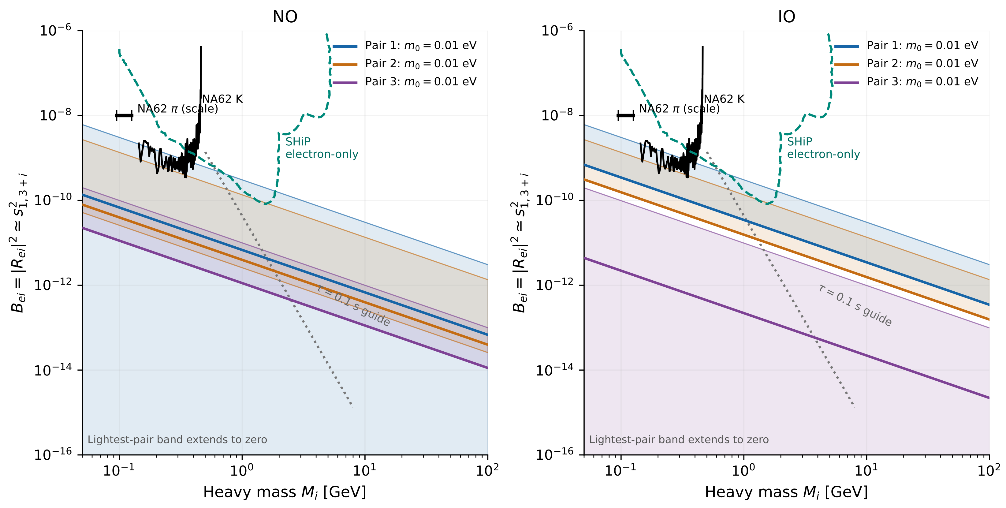
Mixing decreases with $M_i$, while Yukawa strength increases. Equivalently, $m_i=v^2{y}_i^2/M_i$ exactly and $y_i^2=m_i({\widehat{M}}_i+m_i)/v^2$. A small mixing therefore need not imply a weak Yukawa coupling. For $m_i=0.05$ eV, $({\mathcal{U}}_i^2,y_i)$ are approximately $(5\times {10}^{-11},4.1\times {10}^{-8})$ at 1 GeV, $(5\times {10}^{-14},1.3\times {10}^{-6})$ at 1 TeV, and $(5\times {10}^{-23},0.041)$ at ${10}^{12}$ GeV. The exact flavor fractions $B_{\alpha i}/{\mathcal{U}}_i^2={\left|V_{\alpha i}\right|}^2$ are potential tests if a state and its flavor-resolved rates are measured; they are not unique to FSS among form-dominant models.

For the Euler angles, the exact electron-row conversion is

$$s_{16}^2=B_{e3},s_{15}^2={\displaystyle \frac{B_{e2}}{1-B_{e3}}},s_{14}^2={\displaystyle \frac{B_{e1}}{1-B_{e2}-B_{e3}}}.$$

(27)

In the mass range shown in Figure 2, these differ negligibly from $B_{ei}\simeq w_i{m}_i/M_i$. We scan the lightest mass from zero to the laboratory envelope $m_{\beta ,\mathrm{norm}}<0.45$ eV [28], with the rounded inputs of Section 4. This use of the three-neutrino endpoint limit is justified in the illustrated region by the minute FSS nonunitarity and inaccessible heavy states. The shaded bands vary the absolute mass, not a joint statistical confidence region. They do not impose cosmological mass priors, whose interpretation depends on the cosmological model, or a simultaneous three-singlet cosmological likelihood.

Figure 2. Illustrative FSS electron-mixing bands for NO and IO, with fixed rounded oscillation parameters and the laboratory mass envelope specified in the text. Solid curves use lightest mass $0.01$ eV; the lightest-pair lower edge extends to zero. The displayed variable $B_{ei}$ agrees with $s_{1,3+i}^2$ at the stated accuracy. The NA62 kaon-search limit and SHiP projection are extracted from the published vector figures specified in Table 2; the pion marker is an order-of-magnitude reference. The SHiP curve assumes electron-only mixing and is not an FSS detector recast. The gray curve is a lifetime diagnostic with $C_i=1$ and $|V_{ei}{|}^2=0.3$ in Equation (30), not a BBN exclusion.

Figure 2. Illustrative FSS electron-mixing bands for NO and IO, with fixed rounded oscillation parameters and the laboratory mass envelope specified in the text. Solid curves use lightest mass $0.01$ eV; the lightest-pair lower edge extends to zero. The displayed variable $B_{ei}$ agrees with $s_{1,3+i}^2$ at the stated accuracy. The NA62 kaon-search limit and SHiP projection are extracted from the published vector figures specified in Table 2; the pion marker is an order-of-magnitude reference. The SHiP curve assumes electron-only mixing and is not an FSS detector recast. The gray curve is a lifetime diagnostic with $C_i=1$ and $|V_{ei}{|}^2=0.3$ in Equation (30), not a BBN exclusion.

The absence of a large observable nonunitarity signal is immediate:

$${\left(R{R}^{†}\right)}_{ee}=\sum _i{B}_{ei}\le {\epsilon }_e⟹M_i\ge m_i\left({\displaystyle \frac{|V_{ei}{|}^2}{{\epsilon }_e}}-1\right).$$

(28)

Each term is positive. Global heavy-neutrino fits constrain this type of deviation at roughly the ${10}^{-3}$ level, with scenario-dependent correlations [29]. Taking ${\epsilon }_e={10}^{-3}$ only as a reference gives $M_i\gtrsim 15$ eV for $m_i=0.05$ eV and $|V_{ei}{|}^2=0.3$. Extrapolating a high-mass fit to that mass is invalid; the exercise shows why it yields no useful lower bound in its own heavy-mass domain. Conversely, the stated perturbative convention $y_i^2<4\pi$ gives

$$M_i<{\displaystyle \frac{4\pi v^2}{m_i}}=7.6\times {10}^{15}\mathrm{GeV}\left({\displaystyle \frac{0.05\mathrm{eV}}{m_i}}\right).$$

(29)

This is a coupling criterion, not an experimental bound, and does not apply to a decoupled $m_i=0$ column. It lies far beyond the laboratory mass window in the figure.

Table 2. Published comparisons for Figure 2. The kaon limit (Ref. [30], Figure 6) and SHiP projection (Ref. [31], Figure 1) are extracted from the original vector figures; the pion marker summarizes the published scale. Table values are approximate summaries, not constant bounds over an entire interval. The SHiP contour is an electron-only reference.

Reference	Representative Scale	Interpretation
NA62, $K^{+}\to e^{+}N$ [30]	$B_e\sim {10}^{-9}$; $0.144$–$0.462$ GeV	Published 90% CL limits over most of the range, for lifetime $>50$ ns; applicable per resolved long-lived state.
NA62, ${\pi }^{+}\to e^{+}N$ [32]	$B_e\sim {10}^{-8}$; $0.095$–$0.126$ GeV	Published production-search limits; long-lived state assumption.
SHiP projection [31]	$B_e\sim {10}^{-10}$ near 1–$1.8$ GeV	Electron-only Majorana benchmark, $6\times {10}^{20}$ protons on target; FSS has additional flavor couplings and needs a dedicated recast.

Table 2. Published comparisons for Figure 2. The kaon limit (Ref. [30], Figure 6) and SHiP projection (Ref. [31], Figure 1) are extracted from the original vector figures; the pion marker summarizes the published scale. Table values are approximate summaries, not constant bounds over an entire interval. The SHiP contour is an electron-only reference.

Reference	Representative Scale	Interpretation
NA62, $K^{+}\to e^{+}N$ [30]	$B_e\sim {10}^{-9}$; $0.144$–$0.462$ GeV	Published 90% CL limits over most of the range, for lifetime $>50$ ns; applicable per resolved long-lived state.
NA62, ${\pi }^{+}\to e^{+}N$ [32]	$B_e\sim {10}^{-8}$; $0.095$–$0.126$ GeV	Published production-search limits; long-lived state assumption.
SHiP projection [31]	$B_e\sim {10}^{-10}$ near 1–$1.8$ GeV	Electron-only Majorana benchmark, $6\times {10}^{20}$ protons on target; FSS has additional flavor couplings and needs a dedicated recast.

BBN supplies an additional, genuinely cosmological restriction but not a universal electron-mixing line. For sub-electroweak masses a useful dimensional lifetime estimate is

$${\mathsf{\Gamma }}_i=C_i{\displaystyle \frac{G_F^2{M}_i^5}{96{\pi }^3}}{\mathcal{U}}_i^2,{\tau }_i\simeq {\displaystyle \frac{0.29\mathrm{s}}{C_i}}\left({\displaystyle \frac{0.05\mathrm{eV}}{m_i}}\right){\left({\displaystyle \frac{1\mathrm{GeV}}{M_i}}\right)}^4.$$

(30)

Here $C_i$ summarizes accessible channels, flavor weights, and hadronic effects; it is not fixed to unity by the model. A reference lifetime $0.1$ s would correspond to $M_i\gtrsim 1.3C_i^{-1/4}$ GeV for $m_i=0.05$ eV under this estimate. Published BBN calculations find lifetimes below about $0.02$ s for thermalized states above the pion mass [33]; production, reheating history, branching fractions, and the other singlets must be specified before applying their limits. In particular, Equation (30) must not be extrapolated through hadronic thresholds as a precision width or to $m_i=0$ as a decay constraint.

Thus a laboratory envelope is not a fully viable cosmological parameter region. Production searches can constrain individual long-lived states directly, while decay-search and future-facility contours generally depend on the full flavor pattern, lifetime, geometry, and any unresolved states. The reference comparisons identify where further searches may be relevant; they do not establish a discovery reach for exact FSS. In the intended high-scale domain, the mixings and exact-versus-leading corrections are too small for the laboratory effects considered here.

6. Origin and a Leading-Logarithmic Estimate of Alignment Breaking

Exact FSS is used here as a boundary condition at an alignment scale $\mathrm{\Lambda }$, without postulating a unique ultraviolet origin. Flavor models with orthogonal Yukawa columns provide examples: $A_4$ constructions realize form dominance [10], and both $A_4$ and $S_4$ examples can preserve it with nonzero reactor mixing [34]. Charged-lepton diagonalization acts by $Y_{\nu }\mapsto L^{†}{Y}_{\nu }$ with L unitary and leaves H unchanged. It can alter the observed angles without generating a conventional decay source. Neither a particular flavor group nor tri-bimaximal mixing is required by the FSS algebra.

These constructions motivate alignment but do not protect it automatically in the complete interacting theory. With nondegenerate charged-lepton Yukawas, their insertions generally spoil column orthogonality. An all-scale technical-naturalness claim requires a protecting symmetry of the full theory or additional restrictions. Without them, FSS is an exactly solvable, potentially symmetry-motivated boundary condition with calculable radiative departures.

To estimate their size, use the one-loop Standard Model equation above all singlet thresholds, in our convention with flavor rows and singlet columns [35]:

$$16{\pi }^2{\displaystyle \frac{d{Y}_{\nu }}{d\ln \mu }}=\left[{\alpha }_{\nu }\mathbf{1}+{\displaystyle \frac{3}{2}}{Y}_{\nu }{Y}_{\nu }^{†}-{\displaystyle \frac{3}{2}}{Y}_e{Y}_e^{†}\right]Y_{\nu }.$$

(31)

At the aligned boundary the first two terms preserve the diagonality of H. Keeping couplings fixed in the integral and defining $L=\ln (\mathrm{\Lambda }/\mu )>0$ gives, for $i\ne k$,

$$\delta H_{ik}={\displaystyle \frac{3L}{16{\pi }^2}}{\left(Y_{\nu }^{†}{Y}_e{Y}_e^{†}{Y}_{\nu }\right)}_{ik}\simeq {\kappa }_{\tau }{\eta }_i{\eta }_k{y}_i{y}_k{V}_{\tau i}^{\ast }{V}_{\tau k},{\kappa }_{\tau }={\displaystyle \frac{3y_{\tau }^{2}L}{16{\pi }^2}}.$$

(32)

For the numerical estimate only, take $y_{\tau }=1.777/174$ and $\mathrm{\Lambda }/\mu ={10}^4$. Then ${\kappa }_{\tau }=1.83\times {10}^{-5}$ and $|\delta H_{ik}|/\left(y_i{y}_k\right)\le {\kappa }_{\tau }/2\simeq 9.1\times {10}^{-6}$. Terms from running couplings, threshold matching, and the small change of the singlet mass basis are beyond this leading-log estimate. The latter is higher-order here for separated singlet masses; near degeneracy the expansion needs separate treatment.

Inserting Equation (32) into the standard nonresonant flavor structures gives the leading source

$$\begin{array}{cc}\hfill {ϵ}_{i\alpha }^{\left(1\right)}={\displaystyle \frac{{\kappa }_{\tau }}{8\pi }}\sum _{k\ne i}{y}_k^2\{& \mathrm{Im}\left[V_{\alpha i}^{\ast }{V}_{\alpha k}{V}_{\tau i}^{\ast }{V}_{\tau k}\right]f^{\left(1\right)}\left(x_{ki}\right)\hfill \\ \hfill & +\mathrm{Im}\left[V_{\alpha i}^{\ast }{V}_{\alpha k}{V}_{\tau k}^{\ast }{V}_{\tau i}\right]f^{\left(2\right)}\left(x_{ki}\right)\},\hfill \end{array}$$

(33)

up to the overall decay-asymmetry sign convention. The flavor sum of this $O\left({\kappa }_{\tau }\right)$ term vanishes by unitarity. The total source starts at

$${ϵ}_i^{\left(2\right)}={\displaystyle \frac{{\kappa }_{\tau }^2}{8\pi }}\sum _{k\ne i}{y}_k^2\mathrm{Im}\left[{\left(V_{\tau i}^{\ast }{V}_{\tau k}\right)}^2\right]f\left(x_{ki}\right).$$

(34)

For $m_k=0.05$ eV and $M_k={10}^{11}$ GeV, $y_k^2=1.65\times {10}^{-4}$. The prefactors before mixing invariants and loop functions are ${\kappa }_{\tau }{y}_k^2/\left(8\pi \right)=1.20\times {10}^{-10}$ and ${\kappa }_{\tau }^2{y}_k^2/\left(8\pi \right)=2.19\times {10}^{-15}$, respectively. They scale linearly with $m_k{M}_k$ at fixed L and are not upper bounds near resonance. They are common-scale source estimates above the thresholds, not an evolution to each separated decay temperature. These numbers characterize the small Standard Model breaking source, not an observed baryon yield: flavor resolution, washout, thresholds, and transport remain necessary for that prediction.

Cooper, King, and Luhn [36] explicitly implement RG-induced leptogenesis in supersymmetric form-dominant flavor models. Their charged-lepton coefficient and potentially enhanced tau Yukawa differ from Equation (31); their viable baryon asymmetries cannot be transferred numerically to this Standard Model estimate. The common mechanism is the radiative loss of orthogonality. This limited calculation quantifies it without constructing a new flavor model or performing threshold-resolved evolution.

7. Conclusions

The family-separated seesaw ansatz is a consistent, restrictive realization of type-I seesaw. Combined with partial unitarity, it fixes the upper mixing blocks and admits a complete unitary reconstruction up to sterile basis. Its neutrino mass sector consists of three aligned two-state systems. The exact relations distinguish physical Takagi masses from singlet parameters but do not imply large corrections to the usual high-scale approximation.

The conventional leptogenesis cancellation follows from established form dominance. The specific correction to Ref. [9] is that the flavor sum of LNV invariants in its proposed decay source vanishes under the ansatz. This conclusion respects that reference’s distinction between LNV and ordinary-oscillation CP invariants. Individual invariants can remain nonzero; the result applies to the specified common-scale, nonresonant one-loop source.

The corrected heavy-mass formulas satisfy the beta-mass identity and show quantitatively significant discrepancies with the proposed expressions, especially for a small lightest mass in inverted ordering. They remain conditional on active–heavy mixing and do not predict a heavy ordering from the light ordering alone. The numerical illustrations make the very small mixings explicit. The double-beta-decay discussion clarifies the left-chiral propagator projection and the distinction between a mass sum rule and a nuclear amplitude.

Flavor symmetries can motivate aligned boundary conditions, while charged-lepton Yukawa running generally perturbs them. The leading-log estimate exhibits a flavored source linear in the radiative perturbation and an unflavored source quadratic in it. A quantitative baryogenesis prediction or experimental exclusion requires additional dynamical and observational inputs. The main contribution is therefore the exact consistency analysis and correction of the proposed relations, with their practical limitations stated explicitly.

References

- Minkowski, P. μ→eγ at a Rate of One Out of 109 Muon Decays? Phys. Lett. B 1977, 67, 421–428. [Google Scholar] [CrossRef] [Scilit]
- Yanagida, T. Horizontal Gauge Symmetry and Masses of Neutrinos. In Proceedings of the Workshop on the Baryon Number of the Universe and Unified Theories; Sawada, O., Sugamoto, A., Eds.; KEK: Tsukuba, Japan, 1979; pp. 95–99. [Google Scholar]
- Gell-Mann, M.; Ramond, P.; Slansky, R. Complex Spinors and Unified Theories. In Supergravity; van Nieuwenhuizen, P., Freedman, D.Z., Eds.; North-Holland: Amsterdam, The Netherlands, 1979; pp. 315–321. [Google Scholar]
- Mohapatra, R.N.; Senjanović, G. Neutrino Mass and Spontaneous Parity Nonconservation. Phys. Rev. Lett. 1980, 44, 912–915. [Google Scholar] [CrossRef] [Scilit]
- Weinberg, S. Baryon- and Lepton-Nonconserving Processes. Phys. Rev. Lett. 1979, 43, 1566–1570. [Google Scholar] [CrossRef] [Scilit]
- Schechter, J.; Valle, J.W.F. Neutrino Masses in SU(2)⊗U(1) Theories. Phys. Rev. D 1980, 22, 2227–2235. [Google Scholar] [CrossRef] [Scilit]
- Grimus, W.; Lavoura, L. The Seesaw Mechanism at Arbitrary Order: Disentangling the Small Scale from the Large Scale. J. High Energy Phys. 2000, 2000, 042. [Google Scholar] [CrossRef] [Scilit]
- Blennow, M.; Fernández-Martínez, E. Parametrization of Seesaw Models and Light Sterile Neutrinos. Phys. Lett. B 2011, 704, 223–229. [Google Scholar] [CrossRef] [Scilit]
- Xing, Z.-Z. Family-Separated Seesaw Relations of Majorana Neutrinos. arXiv 2026, arXiv:2605.27049v2. [Google Scholar]
- Chen, M.-C.; King, S.F. A4 See-Saw Models and Form Dominance. J. High Energy Phys. 2009, 2009, 072. [Google Scholar]
- Choubey, S.; King, S.F.; Mitra, M. On the Vanishing of the CP Asymmetry in Leptogenesis due to Form Dominance. Phys. Rev. D 2010, 82, 033002. [Google Scholar] [CrossRef] [Scilit]
- Aristizabal Sierra, D.; Bazzocchi, F.; de Medeiros Varzielas, I.; Merlo, L.; Morisi, S. Tri-Bimaximal Lepton Mixing and Leptogenesis. Nucl. Phys. B 2010, 827, 34–58. [Google Scholar] [CrossRef] [Scilit]
- Casas, J.A.; Ibarra, A. Oscillating Neutrinos and μ→e, γ. Nucl. Phys. B 2001, 618, 171–204. [Google Scholar] [CrossRef] [Scilit]
- Chen, Z.-Q.; Hu, X.-H.; Zhou, Y.-L. Exact Parametrization of a Minimal Seesaw Model. Phys. Rev. D 2025, 112, 115032. [Google Scholar] [CrossRef] [Scilit]
- Covi, L.; Roulet, E.; Vissani, F. CP-Violating Decays in Leptogenesis Scenarios. Phys. Lett. B 1996, 384, 169–174. [Google Scholar] [CrossRef] [Scilit]
- Davidson, S.; Nardi, E.; Nir, Y. Leptogenesis. Phys. Rept. 2008, 466, 105–177. [Google Scholar] [CrossRef] [Scilit]
- Fong, C.S.; Nardi, E.; Riotto, A. Leptogenesis in the Universe. Adv. High Energy Phys. 2012, 2012, 158303. [Google Scholar] [CrossRef] [Scilit]
- Abada, A.; Davidson, S.; Ibarra, A.; Josse-Michaux, F.-X.; Losada, M.; Riotto, A. Flavour Matters in Leptogenesis. J. High Energy Phys. 2006, 2006, 010. [Google Scholar] [CrossRef] [Scilit]
- Nardi, E.; Nir, Y.; Roulet, E.; Racker, J. The Importance of Flavor in Leptogenesis. J. High Energy Phys. 2006, 2006, 164. [Google Scholar] [CrossRef] [Scilit]
- Pilaftsis, A.; Underwood, T.E.J. Resonant Leptogenesis. Nucl. Phys. B 2004, 692, 303–345. [Google Scholar] [CrossRef] [Scilit]
- Dev, P.S.B.; Millington, P.; Pilaftsis, A.; Teresi, D. Flavour-Covariant Transport Equations: An Application to Resonant Leptogenesis. Nucl. Phys. B 2014, 886, 569–664, Erratum in Nucl. Phys. B 2015, 897, 749–756. https://doi.org/10.1016/j.nuclphysb.2015.06.015. [Google Scholar] [CrossRef] [Scilit]
- Li, S.-P.; Pilaftsis, A. Low-Scale Leptogenesis from Resonant Thermal Lepton Flavour Coherences. arXiv 2026, arXiv:2604.06493. [Google Scholar]
- Rodejohann, W. On Non-Unitary Lepton Mixing and Neutrino Mass Observables. Phys. Lett. B 2010, 684, 40–47. [Google Scholar] [CrossRef] [Scilit]
- Esteban, I.; Gonzalez-Garcia, M.C.; Maltoni, M.; Martinez-Soler, I.; Pinheiro, J.P.; Schwetz, T. NuFit-6.0: Updated global analysis of three-flavor neutrino oscillations. J. High Energy Phys. 2024, 2024, 216. [Google Scholar] [CrossRef] [Scilit]
- Barry, J.; Rodejohann, W. Lepton number and flavour violation in TeV-scale left-right symmetric theories with large left-right mixing. J. High Energy Phys. 2013, 2013, 153. [Google Scholar] [CrossRef] [Scilit]
- Rodejohann, W. Neutrinoless Double-Beta Decay and Particle Physics. Int. J. Mod. Phys. E 2011, 20, 1833–1930. [Google Scholar] [CrossRef] [Scilit]
- Fang, D.-L.; Li, Y.-F.; Zhang, Y.-Y.; Zhu, J.-Y. Neutrinoless Double-Beta Decay in the Minimal Type-I Seesaw Model: Mass-Dependent Nuclear Matrix Element, Current Limits and Future Sensitivities. J. High Energy Phys. 2024, 2024, 217. [Google Scholar] [CrossRef] [Scilit]
- Aker, M. et al. [The KATRIN Collaboration] Direct neutrino-mass measurement based on 259 days of KATRIN data. Science 2025, 388, 180–185. [Google Scholar] [CrossRef] [Scilit] [PubMed]
- Blennow, M.; Fernández-Martínez, E.; Hernández-García, J.; López-Pavón, J.; Marcano, X.; Naredo-Tuero, D. Bounds on lepton non-unitarity and heavy neutrino mixing. J. High Energy Phys. 2023, 2023, 030. [Google Scholar] [CrossRef] [Scilit]
- Cortina Gil, E. et al. [The NA62 Collaboration] Search for heavy neutral lepton production in K+ decays to positrons. Phys. Lett. B 2020, 807, 135599. [Google Scholar] [CrossRef] [Scilit]
- Wang, Z.S.; Zhang, Y. Updated sensitivities to heavy neutral leptons at the LHC far detectors and SHiP. Phys. Rev. D 2026, 113, 075024. [Google Scholar] [CrossRef] [Scilit]
- Bloch-Devaux, B. et al. [The NA62 Collaboration] Search for heavy neutral leptons in π+ decays to positrons. Phys. Lett. B 2026, 872, 140119. [Google Scholar] [CrossRef] [Scilit]
- Boyarsky, A.; Ovchynnikov, M.; Ruchayskiy, O.; Syvolap, V. Improved big bang nucleosynthesis constraints on heavy neutral leptons. Phys. Rev. D 2021, 104, 023517. [Google Scholar] [CrossRef] [Scilit]
- King, S.F.; Luhn, C. Trimaximal neutrino mixing from vacuum alignment in A4 and S4 models. J. High Energy Phys. 2011, 2021, 042. [Google Scholar] [CrossRef] [Scilit]
- Antusch, S.; Kersten, J.; Lindner, M.; Ratz, M.; Schmidt, M.A. Running Neutrino Mass Parameters in See-Saw Scenarios. J. High Energy Phys. 2005, 2025, 024. [Google Scholar] [CrossRef] [Scilit]
- Cooper, I.K.; King, S.F.; Luhn, C. Renormalisation Group Improved Leptogenesis in Family Symmetry Models. Nucl. Phys. B 2012, 859, 159–176. [Google Scholar] [CrossRef] [Scilit]
Disclaimer/Publisher’s Note: The statements, opinions and data contained in all publications are solely those of the individual author(s) and contributor(s) and not of MDPI and/or the editor(s). MDPI and/or the editor(s) disclaim responsibility for any injury to people or property resulting from any ideas, methods, instructions or products referred to in the content. |
© 2026 by the author. Licensee MDPI, Basel, Switzerland. This article is an open access article distributed under the terms and conditions of the Creative Commons Attribution (CC BY) license.