


Abstract
Blazars are variable at every timescale that has been observed, from minute-scale flares to secular trends spanning decades, and across the whole electromagnetic spectrum from radio to very-high-energy (VHE; GeV) -rays. This variability is not merely a nuisance to be averaged over: it is a time-resolved record of the physical conditions in the jet, and therefore a diagnostic of whether, and how, these sources accelerate particles to the highest energies. This review takes variability itself as its organizing principle. Rather than asking whether a particular blazar subclass accelerates ultra-high-energy cosmic rays (UHECRs), we ask what the amplitude, timescale, spectral evolution, inter-band correlation, and polarization behavior of blazar variability reveal about the underlying particle acceleration, and how that information bears on the production of VHE -rays and the acceleration of UHECRs. We organize the discussion by timescale, from microvariability through secular evolution, and by messenger, treating the electromagnetic light curves, the high-energy neutrino signal, and the (necessarily time-averaged) UHECR flux as complementary probes of the same accelerator. We review how causality arguments applied to rapid flares constrain the size, Doppler factor, and magnetic field of the emission region; how the presence or absence of inter-band correlation discriminates between leptonic and lepto-hadronic scenarios; and why the enormous magnetic time delays of charged cosmic rays sever the temporal link that neutrinos preserve. We close with the prospects that the Cherenkov Telescope Array Observatory (CTAO), the Southern Wide-field Gamma-ray Observatory (SWGO), IceCube-Gen2, and the AugerPrime upgrade open for turning time-domain information into the identification of the astrophysical accelerators of the most energetic particles in the Universe.
1. Introduction
Active galactic nuclei are the compact, luminous cores of galaxies in which a supermassive black hole, of to solar masses, accretes surrounding gas. The accretion flow converts gravitational energy into radiation with an efficiency of order ten percent, far exceeding that of nuclear burning, which is why a region no larger than the Solar System can outshine the entire stellar population of its host galaxy. A minority of AGN, of order ten percent, additionally launch collimated, relativistic outflows, jets, that propagate outward along the black-hole rotation axis and can remain collimated over hundreds of kiloparsecs. The launching mechanism is generally attributed to the extraction of rotational energy from the black hole by magnetic fields threading its horizon, or from the inner accretion disk, in the Blandford–Znajek and Blandford–Payne processes, respectively [1,2,3]. The composition of the resulting outflow remains debated: it may be an electron–positron pair plasma, an electron–proton plasma, or Poynting-flux dominated near the base and progressively converted to kinetic energy further out [3,4]. That question bears directly on the subject of this review, since only a jet carrying protons can accelerate the ultra-high-energy cosmic rays and produce the neutrinos discussed below. What is established observationally is that the emitting material moves with bulk Lorentz factors –50, inferred from the apparent superluminal motion of features in very long baseline interferometry images and from the -ray transparency arguments developed in Section 2. The classification of AGN into radio-loud and radio-quiet, and into the various optical types, is substantially a matter of orientation: the same underlying object presents very differently depending on the angle at which the jet and the obscuring torus are viewed [5].
Blazars occupy the extreme of that orientation sequence: they are the radio-loud AGN whose jets point within a few degrees of the line of sight. The small viewing angle is decisive because relativistic beaming amplifies the apparent luminosity of the non-thermal jet emission by orders of magnitude and, crucially for this review, compresses the observed variability timescales by the same Doppler factor. The result is a class of sources whose defining observational property is variability, rapid, large-amplitude, and present across the entire electromagnetic spectrum and at essentially every timescale that instruments have been able to probe, from a few minutes to several decades, with optical records for the best-studied sources now extending over nearly a century [6,7,8,9]. It is this variability, rather than any single time-averaged spectrum, that carries the dynamical information about how blazar jets accelerate particles, and the premise of this review is that it should be read as a diagnostic rather than treated as noise to be averaged away. A time-averaged spectral energy distribution (SED) can usually be fit equally well by competing physical models; what breaks the degeneracy is how the source changes. The shortest variability timescale places an upper limit on the size of the emitting region, and hence, given a luminosity, on its compactness, the dimensionless ratio that measures the optical depth of the region to internal pair production; the magnetic field and Doppler factor follow only through further, model-dependent assumptions about the emission mechanism; the way flux in one band tracks, or fails to track, flux in another encodes the number of emission zones and the identity of the radiating particles; the rise and decay profiles of flares measure the competition between acceleration, cooling, and escape; and the arrival of a high-energy neutrino during a specific flaring state, as opposed to a quiescent one, tells us when the hadronic machinery switches on. Reading variability this way reframes the central question of blazar physics: instead of asking which sources are accelerators in some static sense, we ask what their time-domain behavior reveals about the acceleration itself.
The connection between variability and acceleration in physics is direct and quantitative. Causality requires that a source varying on an observed timescale cannot be larger than , where is the Doppler factor and z is the redshift [10,11]. The detection of minute-scale variability therefore forces the emission into a very compact region and, through the requirement that this region be transparent to its own -rays, demands large Doppler factors. This is not a marginal effect: -ray flux-halving times of order one minute detected in BL Lacertae with Fermi-LAT imply a bulk Lorentz factor and a minimum Doppler factor of ∼15 from the -opacity argument, placing the emission site at a compact scale within the jet [12]. Very-high-energy (VHE; GeV) observations push this further still: intranight TeV variability from BL Lacertae during its extreme 2022 flaring state constrains the emitting region to cm [13], while minute-scale flares in Mrk 501 and PKS 2155−304 imply Doppler factors of several tens [10,14]. Even in the optical, the two-minute cadence now available from the Transiting Exoplanet Survey Satellite (TESS) has yielded minimum variability timescales of tens of minutes in sources such as 3C 371 and S4 0954+65, tightening the constraints on emission-region size well below a milliparsec [15,16]. Each of these measurements is, at root, a statement about how quickly and how compactly the jet can accelerate and cool its radiating particles. The character of the variability also changes systematically with timescale, and each regime probes different physics: microvariability, or intraday variability (IDV), includes flux changes of a few percent to tens of percent on timescales from minutes to less than a day, probing the most compact and dynamic regions of the jet and the fastest acceleration episodes [6,17,18]; short-term variability, spanning days to months, traces the development and decay of individual flares, whose asymmetry and spectral hysteresis measure the balance of acceleration and cooling [19,20]; and long-term variability, over months to years and decades, is characterized statistically through power spectral density analyzes that reveal red-noise stochastic behavior and, in some sources, claims of quasi-periodicity, as in OJ 287 and PG 1553+113 [21,22,23]. Across all these regimes, the recent proliferation of high-cadence, long-baseline monitoring, from TESS in the optical to the continuous coverage of Fermi-LAT in the GeV band, has transformed variability from a qualitative descriptor into a quantitative tool for constraining jet physics [7,15].
The origin of the high-energy hump of the blazar SED, peaking anywhere from MeV to multi-TeV energies, remains the central open question of blazar physics, and it is precisely here that variability becomes a discriminant. In leptonic models, the high-energy emission is inverse-Compton radiation from the same relativistic electrons that produce the synchrotron hump, scattering either their own synchrotron photons (synchrotron self-Compton, SSC) or an external field [24,25,26]. In hadronic and lepto-hadronic models, relativistic protons contribute through proton synchrotron radiation and through the electromagnetic cascades initiated by photo-meson and Bethe–Heitler interactions [27,28,29,30]. Only the latter class accelerates protons and nuclei to the energies relevant for ultra-high-energy cosmic rays (UHECRs), and only the latter produces the high-energy neutrinos that are the unambiguous signature of hadronic acceleration [31,32,33]. Static SED fits cannot cleanly separate these scenarios, but their temporal signatures differ: in a single-zone SSC model, the X-ray (synchrotron) and -ray (inverse-Compton) light curves are produced by one electron population and should therefore be correlated, often with a quadratic flux-flux relation, so that a departure from this behavior is diagnostic. The clearest such departure is the “orphan” flare, a -ray or TeV outburst with no X-ray counterpart, which is difficult to reconcile with one-zone leptonic models and has been invoked as evidence for a hadronic or multi-zone origin [34,35,36]. Time lags between bands, spectral hysteresis loops traced during a flare, and the rotation or stability of the polarization position angle all add further, dynamical constraints that a time-averaged spectrum simply does not contain [37,38]. Variability, in short, carries information that time-averaged spectra do not about whether a radiatively significant hadronic component is present. The inference runs in one direction only: a decorrelation or a slowly varying hard component can favor hadrons, but no light curve can exclude a subdominant or non-radiating proton population, which may still dominate the escaping cosmic-ray output. This asymmetry recurs throughout the review and is one reason the UHECR question cannot be settled electromagnetically.
The multi-messenger era has made this time-domain argument concrete. The watershed event was the 2017 detection of the ∼0.3 PeV neutrino IceCube-170922A in spatial and temporal coincidence with a -ray flare of the blazar TXS 0506+056, at the ∼ level [39]. The decisive word is temporal: the neutrino arrived while the source was flaring, not during quiescence, which is exactly the behavior expected if the hadronic interactions that produce neutrinos are enhanced when the target photon field and proton content peak. The subsequent identification of an earlier neutrino excess from the same direction during 2014–2015 [40], this time without a contemporaneous -ray flare, only sharpened the puzzle, since it shows that the electromagnetic and neutrino light curves need not track one another, pointing to spatially or temporally decoupled emission zones. Both faces of the TXS 0506+056 story are variability phenomena, and both have driven intense time-dependent lepto-hadronic modeling [41,42,43]. Charged cosmic rays, by contrast, are the one messenger for which the temporal link is broken, and understanding why is central to interpreting any blazar–UHECR connection. Because UHECRs are deflected by Galactic and extragalactic magnetic fields, they arrive delayed relative to photons by an amount that scales as the square of the rigidity-dependent deflection angle; for typical extragalactic field strengths, the delay reaches ∼ years for protons and ∼– years for iron nuclei over ∼100 Mpc [44,45]. No blazar monitoring campaign, and indeed no human observational baseline, can bridge such delays: the UHECRs arriving today were produced during activity states that predate any electromagnetic record of the source. This has a profound consequence for the logic of this review. Whereas neutrinos preserve the time-domain correlation with electromagnetic flares and can therefore be tied to specific variability states, UHECRs can only be associated with sources through time-averaged directional arguments, and even then only after accounting for magnetic deflection. Variability thus enters the UHECR problem not as a correlation to be sought in arrival times, but as a determinant of the time-averaged particle output and, through the physical parameters it constrains, of whether a source clears the acceleration threshold at all. That threshold is set by the Hillas criterion, which requires the accelerator to confine particles magnetically up to the observed energies [46]; the jets and lobes of radio-loud AGN are among the few environments that plausibly satisfy it for energies approaching eV [33,47,48]. On the observational side, the Pierre Auger Observatory has established a large-scale dipole anisotropy above eV at more than , confirming an extragalactic origin [49], and joint Auger–Telescope Array analyzes report intermediate-scale correlations with starburst galaxies and, more weakly, with jetted AGN [50,51]; the eV Amaterasu event reported by the Telescope Array [52], whose arrival direction points toward a local void and which that paper does not associate with any source, has been tentatively linked to a blazar by Das et al. [53], but only under the assumption of Lorentz-invariance-violating propagation. We note this caveat explicitly because the association carries no weight without it. In every case, the physical parameters that decide whether a source can be an accelerator, magnetic field, region size, Doppler factor, proton content, are the same quantities that its variability constrains.
The VHE band is where variability, the leptonic–hadronic question, and the UHECR connection meet most directly. VHE photons from distant blazars are attenuated by pair production on the extragalactic background light (EBL), so observed spectra fold together the intrinsic acceleration physics and the line-of-sight photon field [54,55]. Extreme, hard-spectrum, weakly variable high-synchrotron-peaked blazars are the preferred laboratories for EBL measurement, for constraints on the intergalactic magnetic field through the search for pair-echo cascades, and for tests of exotic photon propagation [56,57]. The temporal dimension is again diagnostic: if a fraction of the hard TeV emission from extreme blazars were produced not in the jet but along the line of sight, through the interactions of escaping UHECRs with background photons, that secondary component would be expected to show little or no variability, in contrast to the rapidly varying primary jet emission [58,59]. The interplay between the intrinsic variability of the accelerator and the steadiness of any propagation-induced component thus provides an independent handle on the hadronic content of the jet.
This review is deliberately organized around variability rather than around a source class or a single messenger. Section 2 surveys the multi-frequency variability phenomenology across all timescales, including microvariability, flares, and secular and quasi-periodic behavior, together with the statistical methods used to quantify it, and explicitly sets out what each observable constrains physically. Section 3 reviews leptonic and lepto-hadronic emission models with an emphasis on their time-dependent signatures and shows how variability observables constrain the parameters most relevant to particle acceleration. Section 4 treats VHE -ray variability, the discriminating role of inter-band correlations, and the distinction between variable primary emission and steady propagation-induced components. Section 5 develops the multi-messenger picture as a time-domain problem, centered on the neutrino–flare connection and on the loss of temporal information for charged cosmic rays. Section 6 then examines how the physical parameters constrained by variability bear on the acceleration of UHECRs and on the anisotropy and composition evidence. Section 7 outlines the prospects opened by CTAO, SWGO, IceCube-Gen2, and AugerPrime for real-time, time-domain multi-messenger astronomy, and Section 8 concludes.
2. Multi-Frequency Variability Across All Timescales
Blazar variability spans roughly seven orders of magnitude in timescale, from minutes to decades, and the physics that can be extracted changes character across that range. It is useful to organize the phenomenology into three loosely defined regimes, microvariability, short-term flaring, and long-term and quasi-periodic behavior, while keeping in mind that these are observational conveniences rather than sharp physical boundaries [6,7]. The unifying thread is that each regime constrains a different combination of the emission-region size, the particle acceleration and cooling rates, and the geometry and number of the emitting zones. Table 1 summarizes the three regimes, the timescales over which each is defined, the instruments typically used to probe them, and the physical quantities each primarily constrains; the sections that follow expand on each regime in turn.
Table 1.
The three variability regimes of blazars, the representative observed timescales, the instruments that probe them, and the physical quantities each regime constrains. The boundaries are observational conveniences rather than sharp physical divisions.
Before turning to the regimes themselves, it is worth recalling the phenomenological framework within which blazar variability is interpreted. Blazars are conventionally divided into flat-spectrum radio quasars (FSRQs), which show broad emission lines, and BL Lacertae objects, whose optical spectra are nearly featureless, and are further ordered by the rest-frame frequency of the synchrotron peak into low-, intermediate-, and high-synchrotron-peaked sources (LSP, ISP, HSP) [60,61,62]. This “blazar sequence” correlates the peak frequency with luminosity and Compton dominance and, although its interpretation as a single physical sequence remains debated, it provides a useful organizing axis because the variability properties themselves vary along it: HSP sources tend to show their fastest and largest-amplitude variability in the X-ray and TeV bands, where their synchrotron and inverse-Compton peaks lie, while FSRQs vary most dramatically in the GeV band [63,64].
The observed synchrotron peak frequency, which defines the LSP/ISP/HSP classification, is set by the Lorentz factor of the peak electron , the magnetic field B, and the Doppler factor through
so that reaching the Hz that defines HSP sources requires very energetic electrons, –, or strong beaming [65,66]. The extreme HSP objects, with synchrotron peaks in the hard X-ray band, are of particular interest here because their hard TeV spectra and clean radiation environments make them the leading candidate hadronic accelerators, and their variability, or notable lack thereof, at the highest energies is a recurring theme of this review.
2.1. Microvariability and Intraday Variability
Microvariability, also called intraday or intranight variability (IDV), refers to flux changes of a few percent to tens of percent on timescales from minutes to less than a day [6,17]. It was first established in the optical [17] and has since been detected across the spectrum, from the optical and X-ray bands to GeV and TeV -rays [18,67]. Its diagnostic value follows directly from causality: a flux change on an observed time scale requires an emission region no larger than , so the shortest observed variability sets the tightest bound on the compactness of the acceleration site [10,11]. Microvariability is, however, intermittent rather than continuous: a 25-year optical monitoring program finds duty cycles of 20–50% depending on the source, with no correlation between the presence of micro-variations and the flux state of the blazar [68]. Individual events are well described as a superposition of synchrotron pulses from turbulent cells energized by a shock, a picture in which pulse widths map directly onto the sizes of the brightest turbulent cells [69].
Quantitatively, the causality bound on the comoving radius of the emitting region reads
where is the observed variability timescale, is the Doppler factor of material moving with bulk Lorentz factor at an angle to the line of sight, and z is the redshift [10,11]. Equation (2) is the single most important relation in this review: it converts a measured timescale directly into an upper limit on the size of the accelerator. Figure 1 illustrates the underlying argument: a region of radius R cannot brighten coherently faster than the time light takes to cross it, so a shorter observed flare implies a smaller accelerator.
Figure 1.
The causality argument that turns a variability timescale into a size limit. A region of radius R cannot vary coherently on a timescale shorter than its light-crossing time, ∼; combined with relativistic beaming this yields the bound of Equation (2). The observed duration of a flare (right) therefore places a direct upper limit on the size of the emitting region (left), so that the minute-scale flares seen in the GeV and TeV bands force extremely compact, highly beamed accelerators. The TikZ code for this schematic was generated with the assistance of Claude (Anthropic; Sonnet 5) from a layout and content specified by the author, and was reviewed and edited by the author.
The advent of high-cadence, space-based optical photometry has sharpened this tool considerably: the two-minute sampling of TESS resolves minimum variability timescales of tens of minutes in 3C 371, probing structure well below a milliparsec [15]; ground-based multi-band monitoring of S4 0954+65 reaches comparable conclusions about the compactness of the optical emission region by a different route [16]. Figure 2 illustrates this capability with the TESS light curve of 3C 371: the densely sampled curve reveals continuous low-amplitude flickering superposed on the longer-term trend, and the inset makes explicit the two-minute cadence and the small per-point uncertainties that make such sub-hour structure measurable in the first place. In the GeV band, the detection of flux-halving times of order of one minute in BL Lacertae with Fermi-LAT pushes the minimum Doppler factor to ∼15 from the requirement that the source be transparent to its own -rays [12].
Figure 2.
TESS SAP_FLUX light curve of the blazar 3C 371, illustrating the intraday variability accessible with high-cadence, space-based optical photometry. The offsets between the different TESS sectors were estimated from the contemporaneous R-band WEBT light curve, converted into arbitrary flux units, and normalized by the mean value. The inset panel zooms onto a one-hour segment of the light curve to illustrate the two-minute observing cadence and the per-point uncertainties. The densely sampled curve resolves continuous low-amplitude flickering on sub-hour timescales, which through the causality bound of Equation (2) constrains the emitting region to well below a milliparsec. Reproduced from Otero-Santos et al. [15].
The transparency requirement translates into a lower bound on the Doppler factor. Demanding that the optical depth of the pair production for a photon of the observed energy satisfies yields
where is the Thomson cross-section, the luminosity distance, the flux of the target photons at the pair-production threshold, and the spectral index of the target field [11]. It is the combination of Equations (2) and (3) applied to minute-scale flares that produces the “Doppler-factor crisis” discussed below.
The interpretation of the very fastest events is not without difficulty, and the tension they create is itself a central result. The ∼200 s flux-doubling time observed during the 2006 giant flare of PKS 2155−304 requires, through the -ray transparency argument, a Doppler factor , far in excess of the values –20 inferred from radio VLBI on parsec scales in the same sources [11,70]. This “Doppler-factor crisis” has driven much of the theoretical work on structured jets discussed in Section 3, since it implies that the emitting material either moves substantially faster than the bulk jet or is organized into small, highly boosted sub-regions [71]. Continuous long-look X-ray monitoring campaigns, beginning with the pioneering ASCA observations of Mrk 421, Mrk 501, and PKS 2155−304, established that even the day-scale flares are frequently limited by the light-crossing time of the region rather than by the acceleration or cooling times, so that the observed variability directly measures the size of the emitting zone [72]. The lesson is general: the more finely time-resolved the observations become, the more severely they constrain the compactness of the accelerator, and the more acute the tension with independent size estimates.
2.2. Short-Term Variability and the Anatomy of Flares
Short-term variability, spanning days to months, is the regime of individual flares, and the shape of a flare is itself informative. The rise and decay of a flare measure the competition between the particle acceleration timescale, the radiative cooling timescale, and the light-crossing and escape times of the region [19]. When cooling dominates the decay, the flare is asymmetric, and the sense of the spectral evolution, whether the flux peaks earlier at higher or lower energies, traces out a hysteresis loop in the hardness-flux plane that distinguishes acceleration-dominated from cooling-dominated episodes [19,20]. Flux-doubling timescales as short as a fraction of an hour have been reported even in luminous flat-spectrum radio quasars such as PKS 1510−089, where the power dissipated in a single rapid flare can represent a substantial fraction of the total jet luminosity, placing strong constraints on the location and compactness of the dissipation zone [73]. The energetics and timing of such flares are the raw material from which the maximum attainable particle energy is inferred.
The direction in which a hysteresis loop is traversed carries specific physical meaning. A clockwise loop in the hardness-flux plane, as observed in Mrk 421 during several X-ray flares, indicates that cooling dominates over acceleration because the highest-energy electrons cool first and the spectrum softens as the flux decays; a counter-clockwise loop signals the opposite, acceleration-dominated case [74,75]. Figure 3 shows the two senses schematically. The near-ubiquitous “harder-when-brighter” behavior of HSP blazars in X-rays, the tendency for the spectrum to harden as the source brightens, is the time-averaged imprint of this same competition, and its systematic study across flares provides a direct handle on the injection and cooling timescales that any successful emission model must reproduce [72,76]. Simultaneous multi-wavelength campaigns that capture both the X-ray and TeV bands during a flare are especially valuable because the correlation (or its absence) between the synchrotron and inverse-Compton components tests the single-zone assumption directly, as discussed further below.
Figure 3.
Schematic hardness–flux hysteresis loops traced during a flare, and their physical interpretation. (a) A clockwise loop indicates that radiative cooling dominates over acceleration: the highest-energy electrons cool first, so the spectrum is hardest on the rise and softens as the flux decays. This sense is observed in Mrk 421 during several X-ray flares [74,75]. (b) A counter-clockwise loop indicates the acceleration-dominated case, in which particles are energized progressively and the spectral hardening lags the flux rise. The sense of the loop is therefore a direct time-domain measurement of which of the two competing timescales, given in Section 2, controls the flare, and it is information that no time-averaged spectrum contains. Axes are schematic; real loops are noisier and frequently incomplete.The TikZ code for this schematic was generated with the assistance of Claude (Anthropic; Sonnet 5) from a layout and physical interpretation specified by the author, and was reviewed and edited by the author.
2.3. Long-Term Variability and Quasi-Periodicity
Long-term variability, over months to years and decades, is best characterized statistically rather than event by event. The power spectral density (PSD) of blazar light curves is generally well described by a red-noise power law, in which the variability amplitude grows toward longer timescales [67,77]. Continuous-time autoregressive moving-average (CARMA) modeling of decade-long daily and weekly Fermi-LAT light curves of a sample of FSRQs recovers a red-noise continuum with low-frequency breaks on timescales of order a year in several sources and, in PKS 1510−089, an additional high-frequency break near nine days, hinting at characteristic timescales that may be tied to the size of the emission region or to the dynamics of the accretion flow [78]. The generic shape of such a PSD, with its two breaks and the flat observational noise level that limits the accessible frequency range, is sketched in Figure 4a. The long-timescale break, of order a year, is naturally associated with the accretion flow, since the jet-launching region is fed by the disk, whereas the shorter timescale may instead reflect processes within the jet itself, with the observed value compressed by the Doppler factor [78]. Systematic studies also find that the FSRQ and BL Lac subclasses separate in PSD slope, with FSRQs showing steeper, more structured variability and BL Lacs showing shallower, more stochastic behavior [67]. The longest available records extend this statistical picture well beyond the Fermi era. Optical light curves assembled from historical photographic plates and modern CCD monitoring now span nearly a century for the best-studied sources, and they show that both the mean brightness and the variability amplitude of individual blazars drift on decadal timescales, with no common trend shared by BL Lac objects and FSRQs [9]. Such baselines matter because they are the only ones long enough to test variability on timescales of years with more than a handful of cycles. Superposed on this red-noise continuum are the more controversial claims of quasi-periodic oscillations, most famously the ∼12-year optical cycle of OJ 287, attributed to a supermassive binary black hole, and the ∼2-year -ray modulation reported in PG 1553+113 [21,22]. The two cases differ in an instructive way: the century-long optical record of OJ 287 covers several cycles of its proposed period [9], whereas the -ray baseline of PG 1553+113 samples only a few. Claims of either kind must nonetheless be assessed against the strong red-noise background, which can mimic periodicity over a limited number of cycles, and this cautionary point motivates the careful statistical treatment discussed below.
Figure 4.
Schematic illustration of the long-term variability diagnostics discussed in the text; curves are illustrative and not fitted to any data set. (a) Power spectral density of a blazar -ray light curve modeled as red noise (solid): flat below a low-frequency break of order , falling as above it and steepening to beyond a possible high-frequency break of order , until it reaches the flat observational noise level (dotted) [78]. The dashed curve represents the 99% envelope of simulated light curves with the same PSD and flux distribution [79]. The shaded band marks frequencies sampled by fewer than ∼5 cycles over a decade-long baseline, where a peak such as the candidate QPO shown is most easily mimicked by red noise. (b) A transient QPO appearing, with a common period P and in phase, in the optical flux and in the polarization, each superposed on independent stochastic variability; the shaded interval marks the few cycles over which the oscillation is active, as in the ∼13 h QPO of BL Lacertae [80]. The pgfplots code was generated with the assistance of Claude (Anthropic; Sonnet 5); the functional forms (a broken power law with breaks at and plus a constant noise level in panel (a), and windowed sinusoids of common period superposed on independent stochastic terms in panel (b)) were specified by the author, who reviewed and edited the output.
Systematic, sample-wide searches have tempered the early enthusiasm for blazar quasi-periodicity. Analyzes of the full Fermi-LAT blazar population find that the number of sources showing formally significant periodicities is broadly consistent with what red-noise fluctuations alone would produce over a decade-long baseline, so individual claims must clear a high bar before they can be regarded as genuine [81]. The most robust way to assess a candidate period is to compare it against large ensembles of simulated light curves that reproduce both the red-noise PSD and the (often log-normal) flux distribution of the real data, using methods that preserve these statistical properties [79]. In the schematic of Figure 4a, this amounts to asking whether a peak rises above the confidence envelope of the simulations; because the red-noise power is largest at low frequencies, where a decade-long baseline samples only a handful of cycles, a years-long candidate period falls precisely where this test is least forgiving. This does not diminish the physical interest of a confirmed quasi-periodicity; a genuine years-long cycle would point to a binary supermassive black hole, jet precession, or magnetohydrodynamic instabilities. However, it does mean that secular variability is most reliably used not to hunt for clocks but to characterize the stochastic processes that dominate the light curves and to separate the jet contribution from any accretion-disk signal [81].
The red-noise caveat applies with full force to long-baseline, few-cycle claims, but it is not the whole story, and a distinct class of transient QPOs deserves separate treatment. These last only a few to roughly ten cycles and were historically dismissed as noise for precisely that reason. What changes the argument is the availability of a second, independent observable. In BL Lacertae, a ∼13 h QPO was detected simultaneously in the optical flux and in the polarization degree and angle during a 2020 outburst, and the authors interpret the signal as the signature of a current-driven kink instability propagating in a magnetically dominated jet [80]. Because the flux and the polarization are not the same measurement, a red-noise fluctuation that mimics a period in one of them has no reason to reproduce the same period, in phase, in the other, as illustrated schematically in Figure 4b. The behavior of the same source on shorter timescales makes this point concrete. In high-cadence optical polarimetry obtained during the 2020–2021 active period of BL Lacertae, the micro-variability of the flux is well described by a superposition of synchrotron pulses from shock-energized turbulent cells, yet the individual pulses show no systematic correlation with either the polarization degree or the polarization angle; the same absence of correlation is recovered when turbulent multi-zone simulations with a predominantly turbulent magnetic field are analyzed in the same way [69]. At the level of stochastic variability, then, flux and polarization behave as effectively independent channels, and a period shared by both, in phase, stands out against that background as a coherent signal rather than a chance alignment. The joint appearance of a common periodicity in two independent channels is therefore an argument of a different kind from the single-light-curve significance tests discussed above, and it is one that the red-noise null hypothesis does not naturally accommodate. This matters for the present review because kink instabilities are also an efficient site of magnetic dissipation and particle acceleration, so a transient QPO identified this way is a direct time-domain diagnostic of the acceleration mechanism rather than merely of the jet’s global geometry. It also suggests that polarimetric monitoring should be treated as an integral part of any periodicity search rather than as a separate programme, a point we return to in Section 7.
2.4. Inter-Band Correlations, Time Lags, and Polarization Variability
The single most powerful discriminant between emission scenarios, however, is not the behavior of any one band but the relationship between bands. In a single-zone SSC model the synchrotron (X-ray) and inverse-Compton (-ray) emission are produced by one electron population, so the two light curves should be correlated, frequently with a quadratic flux-flux relation and with characteristic inter-band time lags set by the energy-dependent cooling [20]. Departures from this expectation are therefore diagnostic. The best known departure is the “orphan” flare, a -ray or TeV outburst with no X-ray counterpart, first seen in 1ES 1959+650 and subsequently in other sources; such events are difficult to accommodate in one-zone leptonic models and have been invoked as evidence for a hadronic or multi-zone origin [34,35,36].
The converse case is in fact considerably more common and deserves equal attention: optical outbursts with no corresponding high-energy counterpart occur frequently in well-monitored sources. Their interpretation is instructive precisely because it need not involve any change in the particle population at all. A leading explanation is geometric. If the jet is inhomogeneous and bent, so that different emitting regions subtend slightly different angles to the line of sight, then a modest change in the orientation of one region alters its Doppler factor and hence its observed flux with no change in the intrinsic emission; because the beaming pattern is energy dependent and the various bands are produced at different locations along the jet, such a geometric event can brighten the optical while leaving the -rays unmoved. This mechanism was invoked to explain the extraordinary 2016–2017 outburst of CTA 102, where a twisted, inhomogeneous jet whose emitting regions progressively align with the line of sight reproduces both the flux and the spectral behavior [82]. Variable Doppler boosting of this kind, and more generally a non-stationary optical jet moving in and out of the line of sight, offers a natural account of decorrelations that would otherwise seem to demand separate particle populations. The lesson for the arguments of this review is a cautionary one: an absent correlation is diagnostic, but it does not by itself select between a second emission zone, a hadronic component, and a purely geometric effect, and distinguishing these requires the polarization and spectral information discussed below rather than the light curves alone.
Polarization adds a further, largely independent axis of time-domain information. The degree and, especially, the position angle of the optical and X-ray polarization vary on the same timescales as the total flux, and smooth rotations of the polarization angle during flares point to ordered, evolving magnetic-field geometries, while erratic behavior indicates turbulence [37]. The constraint tightens considerably when polarization and flux are considered jointly rather than separately. The RoboPol monitoring programme established, on a statistically controlled sample of 40 rotation events in 24 sources, that smooth rotations of the optical polarization angle are related to the nearest -ray flare with time lags consistent with zero, an association unlikely to arise by chance under a random-walk model of the polarization angle [83]. The physical implication is direct: the optical synchrotron emission and the GeV emission must share an emission region, or at least a common magnetic structure, so that whatever reorganizes the field also drives the high-energy flare. This is a constraint that neither the flux light curve nor the polarization curve delivers alone, and it disfavors geometries in which the -rays originate far from the optically polarized zone. It also bears on the optical orphan flares just discussed, since a purely geometric brightening need not be accompanied by any polarization-angle rotation, so the two observables together separate geometric from intrinsic events. Together with the transient QPOs discussed earlier in this section, this illustrates a general point: polarization supplies a second, independent time series, and the strongest time-domain inferences come from requiring a model to reproduce both.
The launch of the Imaging X-ray Polarimetry Explorer (IXPE) has extended this axis into the X-ray band, making the synchrotron polarization of HSP blazars directly measurable. The early finding that the X-ray polarization degree exceeds the optical in sources like Mrk 501 supports an energy-stratified shock-acceleration picture that a time-averaged SED alone could not have revealed [38]. Subsequent observations have made the picture considerably richer, and in doing so have complicated the simple “stable versus rotating angle” diagnostic invoked above. Mrk 421 showed an X-ray polarization angle rotating through more than over five days [84], followed by further episodic rotations with distinct multiwavelength behavior [85]; dense two-week monitoring has since resolved variability in both the polarization degree and the angle on timescales far shorter than a single observation [86]; and six epochs of Mrk 501 reveal a comparably variable picture [87]. The lesson is that the polarization angle is neither simply steady nor simply rotating, and that its diagnostic power lies in the detailed time evolution rather than in a binary classification. This raises the observational bar: distinguishing leptonic from hadronic states polarimetrically will require dense monitoring through a flare rather than a single pointing.
2.5. Statistical Tools for Time-Domain Analysis
Extracting these signatures reliably requires care because the underlying red-noise character of blazar variability makes naive period searches and correlation estimates prone to false positives. The standard toolkit includes the fractional and excess variance for quantifying amplitude, the structure function and the discrete correlation function for characterizing timescales and inter-band lags, the Lomb–Scargle periodogram and wavelet methods for periodicity searches, and CARMA modeling for a statistically rigorous estimate of the PSD in unevenly sampled data [67,78]. In every case, the significance of a claimed timescale or correlation must be evaluated against large ensembles of simulated red-noise light curves with the same sampling and noise properties as the data since sparse or irregular sampling can manufacture spurious features.
It is worth being concrete about the individual tools, since each answers a different question and carries its own pitfalls. The fractional root-mean-square variability amplitude quantifies the integrated variability power above the measurement noise and is the standard way to compare variability amplitudes across bands, but it must be corrected carefully for the Poisson noise that dominates faint sources [88].
Concretely, the fractional root-mean-square variability amplitude is defined as
where is the variance of the light curve, the mean square measurement error, and the mean flux; the subtraction of the noise term is essential, since neglecting it inflates the inferred variability of faint sources [88]. The structure function and the discrete correlation function characterize, respectively, the timescales present in a single light curve and the lags between two, but both are notoriously susceptible to sampling artifacts and can produce spurious breaks or peaks when the data are unevenly spaced. The Lomb–Scargle periodogram and wavelet transforms address periodicity searches in unevenly sampled data, yet their significance can only be assessed against red-noise simulations, not against the naive white-noise null hypothesis. CARMA modeling provides a principled, likelihood-based estimate of the PSD that naturally handles irregular sampling and returns physically interpretable characteristic timescales [78]. Across all of these, the recurring methodological theme is that blazar variability is intrinsically red, so that any claimed timescale, lag, or period is only as trustworthy as the simulations used to establish its significance [79,88]. These methodological caveats set the stage for the physical modeling of the next section, where the observed variability is translated into constraints on the emission mechanism and the acceleration of particles.
3. Time-Dependent Emission Models and What Variability Constrains
The two families of emission models introduced in Section 2, leptonic and lepto-hadronic, make their sharpest, most testable predictions not in the time-averaged SED, which they can both reproduce, but in the temporal domain. This section reviews how each class of model behaves dynamically and how the variability observables translate into constraints on the physical parameters most relevant to particle acceleration. Table 2 summarizes the leptonic and lepto-hadronic scenarios side by side, together with the time-domain observable that most cleanly distinguishes each from the others.
Table 2.
Leptonic versus lepto-hadronic emission scenarios: the radiating particles, the dominant high-energy processes, the associated neutrino output, and the temporal signatures that distinguish them. The final column lists the observables that, in the time domain, most cleanly break the SED-fitting degeneracy.
3.1. Leptonic Models and Their Temporal Signatures
In leptonic models, the entire non-thermal SED arises from a single population of relativistic electrons: synchrotron radiation produces the low-energy hump, and inverse-Compton scattering of the synchrotron photons (SSC) or of an external field (external Compton, EC) produces the high-energy hump [24,25,26,65]. Because one particle population feeds both humps, the model predicts a tight, often quadratic, correlation between the synchrotron and inverse-Compton light curves and specific inter-band lags governed by the energy-dependent electron cooling time. These correlated signatures are frequently observed and constitute the primary success of the leptonic picture. Their failures, however, are equally informative: orphan flares, inter-band lags of the wrong sign or magnitude, and the very fast variability that would require implausibly small regions or extreme Doppler factors all expose the limits of the single-zone assumption and motivate either multi-zone leptonic models or a hadronic contribution [34,36]. A particularly instructive case is the transition between quiescent and flaring states: connecting the low-state SED and the very-high-energy flaring behavior of a source such as Mrk 421 within a purely leptonic framework already requires either a change in the emitting-region parameters or the injection of a fresh, harder electron population, and the way these parameters must evolve to track the observed multi-wavelength variability is itself a strong constraint on the model [89].
The leptonic family itself spans a range of geometries with distinct temporal behavior. In the simplest one-zone SSC model, a single homogeneous region produces both humps, and the physical parameters, the magnetic field B, the region size R, the Doppler factor , and the electron energy distribution are tightly constrained by requiring a simultaneous fit to the two SED peaks and their variability [66,90]. External-Compton models, in which the seed photons come from the accretion disk, the broad-line region, or the dusty torus, are more relevant to FSRQs, where the external fields are strong, and they predict variability tied to the external photon field as well as to the electron population [25,91]. Multi-zone and internal-shock models, in turn, distribute the emission across regions with different parameters, which relaxes the single-zone constraints and naturally accounts for the frequency-dependent lags produced when a disturbance propagates down the jet and successively energizes zones emitting at different frequencies [92,93].
It is worth resisting, however, the common assumption that multiple zones necessarily mean more free parameters. That is true of models in which each zone is fitted independently, but not of those in which the zone structure is generated by a prescription: in the turbulent extreme multi-zone (TEMZ) model, for example, the many cells are populated stochastically from a small number of global parameters, so the parameter count is comparable to that of a one-zone fit while the predicted variability and polarization behavior is far richer [94]. Such models are also testable against data at the level of individual cells. When the micro-variability of simulated TEMZ light curves is decomposed into shock-energized synchrotron pulses, the fit recovers the cell structure that was built into the simulation, and the same analysis applied to BL Lacertae yields pulse statistics and flux–polarization behavior closely matching those of the simulation [69]. The multi-zone description therefore makes predictions that can be checked directly against observed light curves, rather than merely accommodating them. Particle-in-cell simulations go further still, since the particle spectrum is an output rather than an input: a reconnection or shock simulation is specified by the magnetization, the plasma beta, and the composition, and it predicts the electron distribution that one-zone leptonic and hadronic models must instead parameterize by hand [95,96]. On that accounting a PIC-informed model can carry fewer free parameters than the single-zone fits it is often contrasted with, and the real cost of multi-zone approaches is computational and interpretive rather than a loss of predictive power. The relativistic-reconnection “minijet” scenario deserves special mention in the leptonic context because particle-in-cell simulations show that reconnection in magnetically dominated plasma efficiently produces the hard, non-thermal electron spectra required, and the small, fast-moving plasmoids it generates provide a physical realization of the high effective Doppler factors demanded by the fastest flares [95,96].
3.2. Lepto-Hadronic Models and Neutrino Co-Production
In lepto-hadronic models, a population of relativistic protons is co-accelerated with the electrons, and the high-energy emission includes proton synchrotron radiation along with the electromagnetic cascades initiated by photo-meson () and Bethe–Heitler pair-production interactions [27,28,29,30,97,98]. The decisive feature of these models, for the purposes of this review, is that the same interactions that feed the electromagnetic cascade also produce high-energy neutrinos, so the neutrino output is an inescapable corollary of hadronic -ray production. In a interaction, the proton produces charged and neutral pions, whose decay chains channel energy into neutrinos and into the electromagnetic cascade, respectively; the branching between these channels is fixed by particle physics, which is what makes the neutrino flux a quantitative prediction rather than a free parameter once the proton content and target photon field are specified [31,32].
The photo-meson channel proceeds near the resonance as
so that neutral pions feed the electromagnetic cascade while charged pions feed the neutrinos, each neutrino carrying on average ∼ of the parent proton energy [31,32]. The fixed branching in Equation (5) is what ties the neutrino output to the -ray output and makes the neutrino flux a quantitative prediction.
Photo-meson production dominates in the radiation-rich inner jet, but it is not the only hadronic channel, and interactions become competitive wherever the jet encounters dense matter rather than dense radiation. Collisions between the jet and clouds from the broad-line region, or with material stripped from stars crossing the jet, have been proposed as sites of -ray emission [99,100]. Through hadronuclear interactions, they have also been proposed as the origin of the neutrino emission from TXS 0506+056, both for the 2017 event and for the 2014–2015 outburst, which occurred without an accompanying enhancement of the electromagnetic flux [101,102]. The variability signature is set by the dynamics of the obstacle rather than by the light-crossing time of a pre-existing emission zone, and it is not unique to the channel. The penetration of a single cloud produces a relatively slow, non-recurring event, transient in nearby low-luminosity sources such as Centaurus A and steady in powerful FR II jets [99]. Stellar material ablated and accelerated by the jet can instead produce very rapid flares [100], so the time domain alone does not identify an obstacle-driven origin. Interactions at the jet–sheath boundary and with the surrounding medium supply a further, more steady contribution. We note this channel here because it evades some of the constraints developed elsewhere in this review: provided a sufficiently dense target is available, production does not require a dense photon field and is therefore not suppressed in the transparent, weakly radiating jets that Section 6 identifies as the best candidate UHECR accelerators.
The critical point for a review organized around variability is that all of this hadronic machinery, photo-meson and hadronuclear alike, is intrinsically time-dependent, and it need not respond to a flare in the same way as the electromagnetic emission. The neutrino production efficiency depends on the density of the target photon field, which itself rises and falls during a flare; the proton cooling and escape times differ from those of the electrons; and the electromagnetic cascade that reprocesses the -decay -rays introduces its own delays. As a result, the neutrino light curve can lead, lag, or decouple entirely from the photon light curve, and modeling this behavior requires solving the full coupled evolution of protons, secondaries, and photons rather than fitting a static spectrum [42,43].
A further and less widely appreciated complication is spatial. Because protons cool radiatively far more slowly than electrons of the same Lorentz factor, they are not confined to the region in which they were accelerated: over a proton cooling time they can diffuse across, or be advected out of, the compact zone, so the volume in which hadronic emission is actually produced may be substantially larger than the leptonic emission region inferred from the causality bound of Equation (2). The same applies to the cascade. Photons produced at the lower end of the cascade, at and below ∼TeV, have a smaller absorption probability and therefore a longer mean free path, so the effective size of the cascade-emitting region grows as the cascade proceeds down in energy. Both effects act in the same direction on the light curve: they smooth it, lengthening the minimum variability timescale of the hadronic component relative to the synchrotron component and washing out the sharp features that the leptonic emission retains. This is precisely the signature, a hard component varying more slowly than the synchrotron emission, that has been proposed as a time-domain diagnostic of hadronic content [103]. It also cuts the other way as a caution: a one-zone hadronic model that assumes the protons share the electrons’ region and variability timescale is making a strong and usually unstated assumption, and the resulting fits to rapid flares may be correspondingly optimistic. Explicit treatments of proton escape and transport in this context remain relatively few [96,104], and we regard the coupling of spatial transport to time-dependent lepto-hadronic radiation codes as one of the more pressing theoretical needs identified by this review.
This need has driven the development of a generation of time-dependent lepto-hadronic radiation codes that solve the coupled integro-differential “kinetic” equations for the energy distributions of the interacting species, photons, electrons, positrons, protons, neutrons, pions, muons, and neutrinos, as functions of time. Several such codes are now in active use, including AM3, ATHEνA, SOPRANO, the Böttcher–Reimer framework, and LeHa-Paris, among others [29,105,106]. AM3, for example, is a documented open-source tool that has been applied not only to blazars, including the modeling of TXS 0506+056, but also to gamma-ray bursts and tidal disruption events, underlining that the same numerical machinery describes hadronic transients across source classes [105]. For the questions of this review, the value of these codes is precisely that they predict light curves in every channel, so that the observed inter-band and photon–neutrino timing relations can in principle become quantitative tests of the hadronic hypothesis rather than qualitative plausibility arguments.
That promise carries a caveat which, for a review organized around variability, should be stated plainly. Cross-validation of these tools is under way through the Blazar Hadronic Code Comparison Project, which has run a set of leptonic and lepto-hadronic benchmarks, including the non-linear Bethe–Heitler pair-production loop, through independent codes [107]. The published results are described by their authors as preliminary, cover only a small number of steady-state scenarios, and find agreement at approximately the level. This is a meaningful check on the underlying radiative physics, but it is not a validation of the time-dependent predictions, and the distinction matters here: the light-curve shapes, lags, and photon–neutrino timing relations on which the arguments of this review depend have not been compared across codes to the standard that the steady-state spectra have. Until they are, quantitative timing predictions from any single code should be treated with corresponding caution, and a systematic time-dependent comparison would be of considerable value to the observational programme outlined in Section 7.
A concrete application of this machinery to TXS 0506+056 illustrates what is at stake. Cerruti et al. [41] contrast two archetypal single-zone lepto-hadronic solutions for the 2017 high state: one in which the high-energy hump is dominated by proton synchrotron emission, and one “mixed” solution in which it is dominated by synchrotron self-Compton with a subdominant hadronic cascade. Both reproduce the electromagnetic SED comparably well, and no feature of the photon spectrum distinguishes them. Their neutrino predictions, however, differ sharply: narrow and peaking above eV in the proton-synchrotron case, broader and peaking at substantially lower energy in the mixed case. The neutrino channel therefore breaks a degeneracy that is invisible in the photon SED alone, and, since the two solutions also imply different cooling times and hence different light-curve shapes, so in principle does the variability.
Two generic constraints make the lepto-hadronic scenario demanding, and both are sharpened by variability. The first is energetic: reproducing a detectable neutrino flux typically requires proton luminosities that approach or exceed the Eddington luminosity of the central black hole, a tension that becomes acute when the modeling is required to match a specific flaring state rather than a time-averaged spectrum [108,109]. The second is the X-ray cascade constraint. Photomeson interactions produce neutrinos through charged-pion decay and, through neutral-pion decay, pairs that initiate an electromagnetic cascade; Bethe–Heitler pair production, , produces no neutrinos at all but adds to the same pair population. The combined synchrotron emission of these pairs fills the “valley” between the two SED humps, typically in the hard-X-ray to MeV band, so that the observed X-ray flux during a flare places a firm upper limit on the allowed proton luminosity and hence on the neutrino output [110,111].
The efficiency of this process is captured by the photo-meson optical depth , the ratio of the dynamical time to the interaction time, which relates the neutrino luminosity to the proton luminosity through
with set by the size and target photon density of the region [32,109]. The coefficient follows from Equation (5): one third of the pion energy goes into charged pions at the resonance, of which roughly three quarters is carried by neutrinos. The value often quoted in the literature instead assumes the multi-pion regime well above the resonance, where charged and neutral pions are produced in comparable numbers, so that the charged fraction is rather than . Which coefficient applies depends on the target spectrum, and the factor of between them is small compared with the uncertainty in itself. Because R and both vary during a flare, Equation (6) makes explicit why the neutrino light curve need not follow the electromagnetic one. Because both constraints tighten when the source is caught in a well-sampled flare, the time-resolved multi-wavelength data are precisely what turn the hadronic hypothesis from a qualitative possibility into a quantitatively testable, and often severely constrained, model [29,112]. Recent population-level applications, in which a single lepto-hadronic framework is fit to hundreds of Fermi blazars, make this concrete by showing which sources and which flaring states can plausibly contribute to the diffuse neutrino flux without violating the electromagnetic constraints [113].
3.3. From Variability to Jet Parameters
The bridge from variability to physical parameters rests on two arguments applied together. The first is causality, which bounds the comoving size of the emission region through . The second is the requirement of -ray transparency: for the observed VHE photons to escape rather than be absorbed by pair production on the internal soft photon field, the compactness of the region must be low enough, which for a given luminosity and variability timescale sets a lower bound on the Doppler factor [10,11]. Applied to minute-scale flares, these two conditions jointly force to values of several tens and confine the emission to regions of cm or smaller, far more compact than the jet cross-section inferred from radio imaging, a tension that is one of the central puzzles of blazar physics. The same flare timing, combined with the inferred magnetic field, bounds the maximum energy to which particles can be accelerated within a dynamical time, through the competition between the acceleration timescale and the shortest of the cooling and escape timescales, and hence feeds directly into the Hillas-type estimates relevant to UHECR production discussed in Section 6. In the hadronic case this maximum-energy argument is doubly important, because the protons that are not lost to interactions within the source are exactly those that can escape as cosmic rays, so the flare-derived parameters simultaneously constrain the neutrino output and the potential UHECR contribution.
3.4. Structured and Time-Evolving Jets
The compactness tension has driven the development of structured and time-evolving jet models, each of which predicts a distinct variability signature; Figure 5 contrasts the four canonical geometries schematically. In shock-in-jet models a disturbance propagating down the jet energizes successive regions, producing flares whose inter-band lags reflect the frequency-dependent location of the emitting zone [19]. In magnetic-reconnection or “minijet” models the emission arises from small, randomly oriented, relativistically moving plasmoids within the jet, so that the effective Doppler factor of an individual event can greatly exceed the bulk value, naturally accounting for the fastest flares without requiring an extreme bulk Lorentz factor [71,96]. In spine-sheath models a fast inner spine is surrounded by a slower sheath, and the radiative interplay between the two components enhances the target photon field for interactions while producing polarization and variability patterns distinct from the single-zone case [114,115]. Turbulent multi-zone models, finally, reproduce the stochastic, red-noise character of the long-term light curves and the erratic polarization behavior seen in many sources. These geometries also address the multi-messenger timing puzzles directly: a spine-sheath or otherwise multi-zone configuration allows the neutrino-producing region to be spatially and temporally decoupled from the bulk of the electromagnetic emission, which is one way to accommodate a neutrino signal that does not track the -ray light curve. Discriminating among these scenarios is therefore precisely a time-domain problem: they are most cleanly separated by their predicted inter-band correlations, lags, and polarization-angle behavior, and by the relative timing of the neutrino and photon signals, not by any static spectrum.
Figure 5.
Schematic comparison of the four canonical blazar jet geometries invoked to explain the variability phenomenology; in each panel the jet is launched from an accretion disk around the central black hole (left) and diverges to the right. (a) In the single-zone model one homogeneous region produces both SED humps, giving tightly correlated multi-band variability. (b) In the shock-in-jet model a disturbance propagating down the jet successively energizes different zones, producing frequency-dependent inter-band lags. (c) In the minijet/plasmoid model, magnetic reconnection generates small, randomly oriented, relativistically moving plasmoids whose high local Doppler factor accounts for the fastest flares without an extreme bulk Lorentz factor. (d) In the spine-sheath model a fast inner spine is surrounded by a slower sheath; the radiative interplay enhances the target photon field and allows the neutrino-producing region to be spatially decoupled from the bulk electromagnetic emission. The four scenarios are most cleanly distinguished not by their time-averaged spectra but by their predicted inter-band correlations, lags, polarization behavior, and neutrino–photon timing. The TikZ code for this schematic was generated with the assistance of Claude (Anthropic; Sonnet 5) from a layout and content specified by the author, and was reviewed and edited by the author.
A promising recent direction is the explicit search for hadronic signatures in the time domain, rather than in the time-averaged SED. Because the proton cooling and cascade timescales differ systematically from the electron cooling times, a hadronic contribution should leave characteristic imprints on the relative timing and shape of the multi-wavelength light curves, for example, a hard component that varies more slowly than the synchrotron emission, or a specific pattern of lags between the X-ray, GeV, and TeV bands [103]. Applying this approach to well-monitored sources such as Mrk 501 illustrates both its promise and its difficulty: the predicted hadronic timing signatures are subtle and require dense, simultaneous, multi-band coverage of the kind that only the next generation of facilities will routinely provide, which is one of the motivations for the observational program outlined in Section 7.
3.5. From Parsec-Scale Knots to the Radiating Particles
It is worth making explicit a distinction that the preceding discussion has used implicitly, because it joins two bodies of work that are usually pursued separately. On one side is the radio and millimeter VLBI literature, which images the jet on parsec scales, tracks the proper motions of discrete bright knots, and derives the bulk Lorentz factors, viewing angles, and jet kinematics of large samples [116,117]. On the other is the high-energy SED and variability literature reviewed in the preceding sections, which infers the energy distribution of the radiating particles, the magnetic field, and the compactness of the emitting region from spectra and light curves that carry no spatial information at all. The first measures where the emitting material is and how fast it moves in bulk; the second measures how energetic the particles inside it are. These are entirely different quantities, differing by three to five orders of magnitude in Lorentz factor, and the double-humped blazar SED requires both. Because the two communities work with different instruments, different resolutions, and largely different timescales, the relationship between their respective quantities is often left implicit, and this subsection sets it out.
What VLBI resolves, at radio and in a handful of sources optical wavelengths, is a sequence of discrete bright features, knots or plasmoids, that emerge from the core and propagate outward along the jet. Their apparent transverse speeds routinely exceed c, the classic superluminal signature, which for a feature moving at angle to the line of sight implies and constrains to a few degrees. This is the macroscopic scale: a parsec-sized region of magnetized plasma in bulk relativistic motion, whose Doppler factor sets the beaming and the compression of observed timescales that Equation (2) exploits.
Within such a knot, however, the radiating particles carry individual Lorentz factors far larger than the bulk value. Producing a synchrotron peak in the optical or X-ray band requires, through Equation (1), electron Lorentz factors – for LSP sources and – for the HSP class, that is, three to five orders of magnitude above . The two humps of the blazar SED then follow directly from this single population: the same electrons radiate synchrotron photons in the field threading the knot, producing the low-energy hump, and inverse-Compton scatter those photons, or an external field, to produce the high-energy hump. Each scattering boosts the photon energy by roughly in the comoving frame, which is why an optical seed photon and a electron yield emission in the GeV–TeV band, and the whole spectrum is then Doppler boosted by into the observer frame. The factor and the factor therefore play quite different roles: the former determines what we see and how fast it appears to change, the latter determines the energies at which the two humps sit.
The connection is not merely conceptual; it has a time-domain expression that is directly relevant here. Several sources show -ray flares coincident, within the timing uncertainties, with the passage of a new superluminal knot through the millimeter VLBI core, which places the high-energy dissipation site parsecs from the black hole rather than in the compact sub-parsec region assumed by many one-zone fits [93,116]. Conversely, the minute-scale variability of Section 4 demands emission regions many orders of magnitude smaller than a resolved knot, which is the compactness tension restated in spatial terms: the imaged jet and the flaring region cannot be the same object. The plasmoid picture of Section 3 offers a natural reconciliation, with the resolved knot containing many small, independently moving sub-regions whose local Doppler factors exceed the bulk value. In that view, the macroscopic and microscopic descriptions are nested rather than competing, and the observational program is to determine how the particle acceleration is distributed within the resolved structure, a question that polarimetric imaging and time-resolved spectroscopy are only now beginning to address.
4. Very-High-Energy Gamma-Ray Variability and Propagation
4.1. Minute-Scale TeV Flares and Extreme Accelerators
The VHE band occupies a special place in this review because it is where the fastest variability, the largest variability amplitudes, the hardest spectra, and the most direct connection to the highest-energy particles all converge. The amplitude deserves to be stated alongside the timescale, since the two are distinct properties and the second is often overlooked. In high-synchrotron-peaked sources the fractional variability amplitude of Equation (4) increases systematically with photon energy: the same source that varies by tens of percent in the optical varies by factors of a few in X-rays and by an order of magnitude or more at TeV energies [67,74]. The reason is that the highest-energy photons are produced by particles on the steeply falling tail of the energy distribution, which respond non-linearly to any change in injection or cooling; a modest shift in the maximum particle energy produces a large change in TeV flux while barely moving the optical. The VHE band is therefore not only the fastest but also the most sensitive probe of the acceleration process, which is why its light curves carry disproportionate weight in the arguments that follow.
The shortest variability timescales are measured at high energies generally. The current records sit in the GeV band, where flux-halving times of order one minute have been reported in BL Lacertae with Fermi-LAT [12], with the TeV band close behind and supplying the best-resolved events. The giant flare of PKS 2155−304 observed by H.E.S.S. on MJD 53944 reached fluxes of up to ∼15 times that of the Crab Nebula and displayed well-resolved bursts varying on timescales of ∼200 s, with a fractional rms variability amplitude twice that seen in archival X-ray data from the same source, a direct illustration of the energy dependence just described. Its light curve was characterized by decomposing it into a constant level plus a superposition of individual bursts with asymmetric rise and decay times of a few minutes [10], a procedure sketched in Figure 6a. Comparably fast variability has also been seen in Mrk 501 and in BL Lacertae during its extreme 2022 outburst [10,13,14]. Such events impose the most stringent causality and transparency constraints available: applied through Equations (2) and (3), the fastest bursts force Doppler factors of several tens and emission regions smaller than cm, and they probe the acceleration mechanism at its most extreme, where particles must be energized on timescales approaching the light-crossing time of the region. Indeed, if the emitting region is assumed comparable to the Schwarzschild radius of the central black hole, with a mass of –, the observed timescales require Doppler factors of ∼50–100 or more, sharpening the “Doppler-factor crisis” introduced in Section 2 [10]. Figure 6b shows how the two conditions combine in the plane of emission-region size and Doppler factor: causality confines the region to lie below a line whose normalization is set by the variability timescale, transparency excludes the most compact and least boosted configurations, and the Schwarzschild radius can be reached only at the high- end of the allowed wedge. Table 3 collects this and the other benchmark sources discussed throughout the review, together with their classification, redshift, and fastest reported variability timescale, to serve as a quick reference for the case studies that follow.
Figure 6.
Schematic illustration of the constraints imposed by minute-scale VHE flares; curves are illustrative and not fitted to any data set. (a) A flaring VHE light curve (solid) decomposed into a constant level plus a superposition of individual bursts (dashed) with asymmetric rise and decay times of a few minutes, the procedure used to characterize the giant flare of PKS 2155−304 [10]. (b) Allowed range of emission-region size R and Doppler factor for a variability timescale s at : causality (Equation (2)) excludes the region above the solid line, while transparency (Equation (3), shown schematically) excludes the region below the lower curve. The grey band marks the Schwarzschild radius of a – black hole; an emission region of that size is compatible with causality only for –110 (dotted lines), which is the origin of the “Doppler-factor crisis”. The pgfplots code was generated with the assistance of Claude (Anthropic; Sonnet 5); the causality bound (for s and ), the Schwarzschild-radius band, and the burst profiles were specified by the author, who verified the plotted numerical values and reviewed and edited the output.
Table 3.
Representative blazars discussed in this review, with their classification, redshift, the fastest reported variability timescale, and their significance for the variability–acceleration connection. Values are indicative and drawn from the cited literature; the fastest timescales in particular are flare-state dependent.
4.2. EBL Attenuation and the Gamma-Ray Horizon
Interpreting VHE spectra requires accounting for propagation because VHE photons from distant blazars are attenuated by pair production on the extragalactic background light (EBL). The observed spectrum is therefore the product of the intrinsic emission and an energy- and redshift-dependent absorption factor set by the EBL density [54,55]. This attenuation is both a complication and an opportunity: because the intrinsic hard spectra of extreme, weakly variable HSP blazars are relatively well understood, these sources serve as standard candles for measuring the EBL and the cosmic -ray horizon, and their steadiness is what makes them usable for this purpose [57]. Separating the intrinsic spectral shape from the absorbed one is essential before any hard TeV tail can be interpreted as evidence for exotic physics or a hadronic component.
The use of blazars as EBL probes has matured into a precision measurement. The first detections came from Fermi-LAT, statistically stacking the GeV spectra of many blazars across redshift, and from the ground-based Cherenkov telescopes using the brightest individual TeV sources; both recovered the absorption imprint and reconstructed a cosmic optical and infrared background in good agreement with the integrated light of galaxy surveys [119,120]. The subsequent decade has consolidated this considerably. The Fermi-LAT analysis of more than 700 blazars detects the attenuation at greater than and traces the EBL evolution out to [121]; H.E.S.S. has produced a largely model-independent determination of the EBL spectrum and the cosmic -ray horizon from its brightest sources, without assuming a parameterized background model [122]; and a joint MAGIC and Fermi-LAT analysis extending to finds the observed opacity consistent with standard EBL absorption, with no evidence for the anomalous transparency that axion-like particles or line-of-sight cascades would produce [123].
This matters for the present review in three ways. First, it means that the intrinsic, absorption-corrected spectra of distant blazars can be recovered with confidence, which is a prerequisite for identifying any anomalous hard tail. Second, the very hardness of the corrected spectra of extreme HSP sources such as 1ES 0229+200, with photon indices harder than standard shock acceleration predicts even after de-absorption, is one of the persistent puzzles that hadronic and line-of-sight cascade models were invoked to explain [55,59]. Third, and cutting the other way, the absence of anomalous transparency bounds how much of any hard TeV tail can be attributed to secondary emission produced along the line of sight rather than in the jet [123], which tightens the argument of Section 4 where we use the steadiness of such a component as a diagnostic of hadronic content. The EBL is thus simultaneously a foreground to be removed and, once removed, a revealer of the intrinsic spectral shape that carries the acceleration physics.
4.3. Variable Primary Versus Steady Secondary Emission
That separation leads to the most direct connection between VHE emission and UHECR acceleration. If a fraction of the hard TeV flux from extreme blazars were produced not in the jet but along the line of sight, through the interactions of escaping ultra-high-energy protons with background photons, that secondary component would have a characteristic signature: it would be steady because the cosmic-ray-induced cascade is smeared over the long propagation path and cannot follow the rapid variations of the jet [58,59]. The same escaping protons, deflected by the intergalactic magnetic field (IGMF), would also seed an electromagnetic cascade whose delayed, extended “pair-echo” emission constrains the IGMF strength through its non-detection around sources such as 1ES 0229+200 [56].
The pair-echo argument has an explicitly temporal dimension that reinforces the theme of this review. The secondary GeV emission produced when TeV photons initiate an electromagnetic cascade in the intergalactic medium is not only spatially extended but also time-delayed, because the intervening magnetic field lengthens the path of the intermediate pairs before they up-scatter cosmic-microwave-background photons back into the GeV band [124]. The magnitude of this delay depends on the IGMF strength, so that the joint analysis of the prompt TeV and delayed GeV emission from a variable source constrains the field: a strong field spreads the echo over such long timescales that it is diluted below detectability, while a weak field would produce a detectable, delayed GeV counterpart to TeV flares. The non-detection of such echoes around hard-spectrum blazars thus places a lower bound on the IGMF, and it does so through a fundamentally time-domain measurement, the comparison of the variable primary and the smeared, delayed secondary [56,124]. This is the same logic, applied to electromagnetic cascades, that distinguishes variable jet emission from steady cosmic-ray-induced emission earlier in this section. The temporal contrast is thus a diagnostic in its own right: a rapidly varying hard TeV component is intrinsic and jet-based, whereas a steady, non-varying hard tail in a distant source is the expected signature of line-of-sight UHECR interactions. Variability, once again, discriminates between a leptonic and a hadronic origin for the highest-energy photons.
5. The Multi-Messenger Picture as a Time-Domain Problem
The multi-messenger connection between blazars and the highest-energy particles is fundamentally a question of timing, and the three messengers, photons, neutrinos, and cosmic rays, carry very different temporal information. Photons and neutrinos travel in straight lines at the speed of light and therefore preserve the time structure of their source; charged cosmic rays do not. Organizing the multi-messenger evidence around this distinction clarifies both what has been learned and what can and cannot be learned from time-domain correlations.
5.1. The Neutrino–Flare Connection: TXS 0506+056
The foundational event is the 2017 coincidence of the ∼ PeV neutrino IceCube-170922A with a -ray flare of TXS 0506+056, significant at the ∼ level [39]. The essential point is temporal: the neutrino arrived while the source was flaring in -rays, exactly as expected if the hadronic interactions that produce neutrinos are enhanced when the jet’s proton content and target photon field peak. The event triggered an intensive modeling effort, and a robust conclusion emerged from it: single-zone lepto-hadronic fits to the flaring state require proton luminosities that strain the jet’s energy budget and tend to overproduce the X-ray flux through the accompanying electromagnetic cascade, so that the X-ray light curve during the flare becomes a stringent constraint on the hadronic component [41,42,108]. This behavior is not unique to the 2017 event. Figure 7 shows the multi-wavelength light curve of TXS 0506+056 across a dedicated 2017–2019 monitoring campaign, from the VHE -rays down to the radio band: the source again displays -ray flaring, most prominently in December 2018, while at lower energies no significant variability is seen over the same interval [125]. The flare, in other words, is not merely the backdrop to the neutrino detection; its multi-wavelength time profile, and in particular the recurring contrast between the active -ray band and the comparatively quiet lower-energy bands, is what constrains the physics.
Figure 7.
Multi-wavelength light curve of TXS 0506+056 during the 2017–2019 monitoring campaign. From top to bottom: MAGIC (VHE -rays), Fermi-LAT (high-energy -rays), X-rays (Swift-XRT and NuSTAR), Swift-UVOT, optical (ASAS-SN, KVA, REM, Siena), and radio (OVRO and Metsähovi). The dotted light-blue line marks the arrival time of the IceCube-170922A neutrino, and the dashed grey line the end of the earlier data set of Ansoldi et al. (2018). The source shows renewed -ray flaring, most prominently in December 2018, while no significant variability is seen in the optical, UV, X-ray, or radio bands over the same interval. This recurring contrast, between an active -ray channel most directly tied to any hadronic cascade and quiet lower-energy bands, is the observable that both motivates a hadronic component and, through the X-ray cascade constraint of Equation (6), limits its luminosity. Reproduced from Acciari et al. [125].
The modeling effort that followed the 2017 event converged on a specific and instructive tension. Single-zone lepto-hadronic fits that reproduce the observed neutrino flux tend to require proton luminosities orders of magnitude above the Eddington limit and to overproduce the simultaneous X-ray flux through the accompanying cascade, so that the very data that make the association compelling also constrain the hadronic component severely [42,108,110]. A further complication is that TXS 0506+056, although observed as a BL Lac, was subsequently argued to be a “masquerading” BL Lac, intrinsically an FSRQ whose broad lines are swamped by the boosted jet continuum, which would supply a hidden external photon field that enhances neutrino production and eases, though does not eliminate, the energetic tension [118].
The broader statistical context comes from stacking analyses, which sum the sub-threshold neutrino signal from many blazars and find that the resolved Fermi blazar population can account for at most a fraction of the diffuse neutrino flux, implying that efficient neutrino production is not a generic property of all blazars but is confined to particular sources or particular flaring states [126,127]. Independent lines of evidence keep the blazar–neutrino connection active while underscoring that it is the time-domain coincidences, such as the 2017 flare, that carry the most weight [128,129]. Several of these are themselves variability results. Radio monitoring with OVRO and Metsähovi finds that blazars coincident with IceCube events tend to be in an elevated or rising radio state at the time of arrival, at the ∼ level [130]. A subsequent analysis with an updated neutrino catalog, a signalness-weighted statistic, and optical as well as radio light curves recovers a correlation of at least only when the IceCube error regions are enlarged to allow for unknown systematics, and none when the published regions are used [131], so the radio–neutrino connection remains suggestive rather than established. More pointedly for the present review, blazars associated with neutrinos show systematically stronger jet beaming than other radio-bright sources in the complete MOJAVE sample, with larger Doppler and Lorentz factors and smaller viewing angles, which the authors take to indicate that neutrino production occurs at sub-parsec distances, where the jet has already been accelerated [132]. Since the most strongly beamed sources are also those in which intrinsic variability is most compressed in time and amplified in flux, this suggests, if the association holds, that the neutrino-producing population is selected by the same property that makes the time-domain approach viable in the first place.
5.2. The 2014–2015 Orphan Neutrino Excess
The picture was complicated, productively, by the archival discovery of an earlier neutrino excess from the same direction during 2014–2015, at significance and comprising roughly a dozen events, but this time without a contemporaneous -ray flare [40]. This “orphan” neutrino episode is the neutrino-channel analogue of the orphan -ray flares discussed earlier, and it carries the same lesson: the electromagnetic and hadronic light curves need not track one another. If neutrinos can be produced copiously while the source is quiescent in -rays, then the emission zones responsible for the two channels must be at least partially decoupled, whether spatially (as in spine-sheath geometries) or through a high internal opacity that hides the accompanying -rays. The mismatch between the neutrino and photon time profiles is thus a direct probe of the jet’s internal structure.
TXS 0506+056 is not the only candidate association, and the others reinforce the same time-domain logic. The PeV-energy cascade event IceCube-35 (“Big Bird”) was found to be temporally coincident with a major outburst of the FSRQ PKS 1424−418, whose integrated electromagnetic energy output during the flare was sufficient to power the neutrino, although the large angular uncertainty of cascade events limits the significance [133]. A separate search identified a track-like event coincident with the blazar GB6 J1040+0617 in a relatively modest activity state, and the associated modeling again ran into the Eddington-limit problem, reinforcing the conclusion that efficient neutrino production requires either special sources or special states [134]. In every case the strength of the association rests on the temporal coincidence between the neutrino and an electromagnetic feature, which is exactly the information that, as argued throughout this review, the neutrino channel preserves and the cosmic-ray channel does not.
5.3. Neutrinos Preserve Time, Cosmic Rays Do Not
The situation for cosmic rays is qualitatively different, and this difference is the crux of the multi-messenger argument. Because UHECRs are charged, they are deflected by Galactic and extragalactic magnetic fields, and the resulting path-length increase delays their arrival relative to photons by an amount that scales as the square of the rigidity-dependent deflection angle. For plausible extragalactic field strengths the delay reaches ∼ years for protons and ∼– years for iron nuclei over a ∼100 Mpc path [44,45].
Quantitatively, a cosmic ray of energy E and charge Z traversing a distance d through a turbulent field of strength B and coherence length is deflected by an RMS angle
and arrives delayed relative to a photon by
which evaluates to ∼ yr for protons and ∼– yr for iron over ∼100 Mpc [44,45]. Equation (8) is the formal statement of why the cosmic-ray channel carries no usable timing information: the delay dwarfs any conceivable monitoring baseline. Figure 8 summarizes this asymmetry schematically: photons and neutrinos leave the flaring jet and travel in straight lines, arriving with the time structure of the flare intact, whereas the charged cosmic ray is scattered by the intervening magnetic field and arrives smeared and delayed by a time that, per Equation (8), exceeds any human monitoring baseline by orders of magnitude.
Figure 8.
Schematic of the multi-messenger time-domain asymmetry that underlies this review. Photons () and neutrinos () leave the flaring blazar jet and propagate in straight lines, so they reach the observer with the time structure of the flare preserved and can be tied to a specific variability state. The charged ultra-high-energy cosmic ray (UHECR), by contrast, is scattered by the intervening Galactic and intergalactic magnetic fields; its arrival direction is smeared following Equation (7) and its arrival time is delayed following Equation (8) by ∼– yr, far longer than any monitoring baseline. Neutrinos therefore probe the accelerator in the time domain, whereas cosmic rays can be associated with sources only through directional, time-averaged arguments. The TikZ code for this schematic was generated with the assistance of Claude (Anthropic; Sonnet 5) from a layout and content specified by the author, and was reviewed and edited by the author.
No monitoring campaign can bridge such intervals: the UHECRs arriving today were produced during activity states that long predate any electromagnetic record of the source, and the flux we receive reflects a time-average over the delay timescale rather than any instantaneous state. The consequence for methodology is decisive. Whereas neutrinos can be tied to specific flares and thus to specific variability states, any blazar–UHECR association must be directional and time-averaged, and it must fold in the smearing of arrival directions by magnetic deflection. Variability enters the UHECR problem not as an arrival-time correlation to be sought, but as the determinant of the time-averaged particle output and of the physical parameters that decide whether a source can accelerate particles to the required energies at all.
6. Variability-Constrained Parameters and the UHECR Connection
6.1. The Hillas Criterion in Variable, Beamed Sources
Having established that the UHECR connection cannot be made in the time domain directly, we now examine how the parameters that variability does constrain feed into the question of whether blazars accelerate the highest-energy cosmic rays. The link runs through the Hillas criterion, which requires that the accelerator confine particles magnetically up to the observed energy, so that the maximum rigidity scales with the product of the magnetic field strength and the size of the acceleration region [46]. Both of these quantities are exactly what rapid variability constrains: the causality and transparency arguments of Section 3 and Section 4 bound the size R and the Doppler factor , and the SED modeling that accompanies a well-sampled flare bounds the magnetic field B. A blazar caught in a minute-scale flare, with cm and the correspondingly high inferred field, sits in a very different part of the Hillas plane from the same source modeled in quiescence, so the variability state directly affects the inferred maximum energy.
In its beamed form the Hillas criterion bounds the maximum energy of a particle of charge accelerated in a region of comoving field B and size R as
where is the shock velocity in units of c [46,135]. The quantities on the right-hand side are constrained to differing degrees, and it is worth being precise about which, since the strength of the whole argument rests on it. Equations (2) and (3) bound R and directly from the observed variability timescale, with no assumption beyond causality and transparency; these are the two robust links between the time domain and the acceleration question. The magnetic field is not measured by the variability at all. It is inferred from broadband SED modeling, through the ratio of the synchrotron and inverse-Compton peak luminosities and frequencies, and is therefore only as reliable as the emission model assumed, with values differing by an order of magnitude between one-zone SSC and external-Compton fits to the same source. The variability enters this inference indirectly, by fixing the R and that the SED fit must adopt, but the dependence is a mediated one. The shock velocity is not constrained observationally in these sources and is conventionally set to order unity for relativistic shocks. So of the four factors, two follow from the variability with few assumptions, one is model-dependent, and the fourth is assumed, and any statement about inherits that hierarchy.
Figure 9 places this relation in its classic graphical form, the Hillas diagram of magnetic field strength against source size, on which the diagonal lines mark the locus required to confine protons and iron nuclei at eV. The blazar region sits close to the proton threshold, so that the precise position of a given source, set by the field and size inferred as above, determines on which side of the line it falls, and hence whether it can accelerate protons to the highest energies or only heavier nuclei. Since the horizontal axis is fixed by the variability while the vertical axis is model-dependent, the dominant uncertainty in placing a source on this diagram is the magnetic field rather than the size.
The Hillas criterion is a necessary but not sufficient condition, and the additional requirements sharpen the role of the variability-derived parameters. Beyond mere magnetic confinement, a viable UHECR accelerator must also satisfy an energetic condition, the jet must carry enough power to supply the observed cosmic-ray luminosity, and the accelerated particles must be able to escape the source without catastrophic losses [135,136]. Here the clean radiation environments of HSP blazars become an asset: because their jets are relatively free of the dense external photon fields that would photodisintegrate nuclei or drain protons through interactions, particles accelerated in an HSP jet can in principle escape as UHECRs, whereas the same dense fields that make FSRQs efficient neutrino factories tend to suppress UHECR escape [47,137]. This is a direct trade-off between the two hadronic messengers, and it means that the source classes best suited to producing neutrinos and those best suited to releasing UHECRs need not coincide. The variability-derived parameters enter on both sides of this trade-off, since they fix the compactness and photon density that determine both the efficiency and the escape probability [138]. Explicit attempts to connect blazar populations to UHECR arrival directions, folding in these considerations, have found suggestive but not yet decisive correlations [138].
Figure 9.
Hillas diagram of magnetic field strength B against characteristic size R for candidate cosmic-ray accelerators, from compact Galactic objects (white dwarfs, neutron stars, Wolf–Rayet stars, micro-quasars, supernovae) through AGN, gamma-ray bursts, and blazars to the largest and weakest-field environments (starburst winds, AGN lobes, galaxy clusters, and the intergalactic medium). The diagonal lines indicate the threshold required to confine a particle at eV, following Equation (9): red for protons () and blue for iron (), with solid lines for relativistic () and dashed lines for slow () shocks. A source must lie above and to the right of the relevant line to reach eV. The blazar region sits close to the proton threshold, so that its precise placement determines whether it can accelerate protons or only heavier nuclei. The horizontal coordinate follows from the variability through Equations (2) and (3), while the vertical coordinate rests on SED modeling and is correspondingly the more uncertain of the two. Figure generated by the author using the HillasPlot software [139].
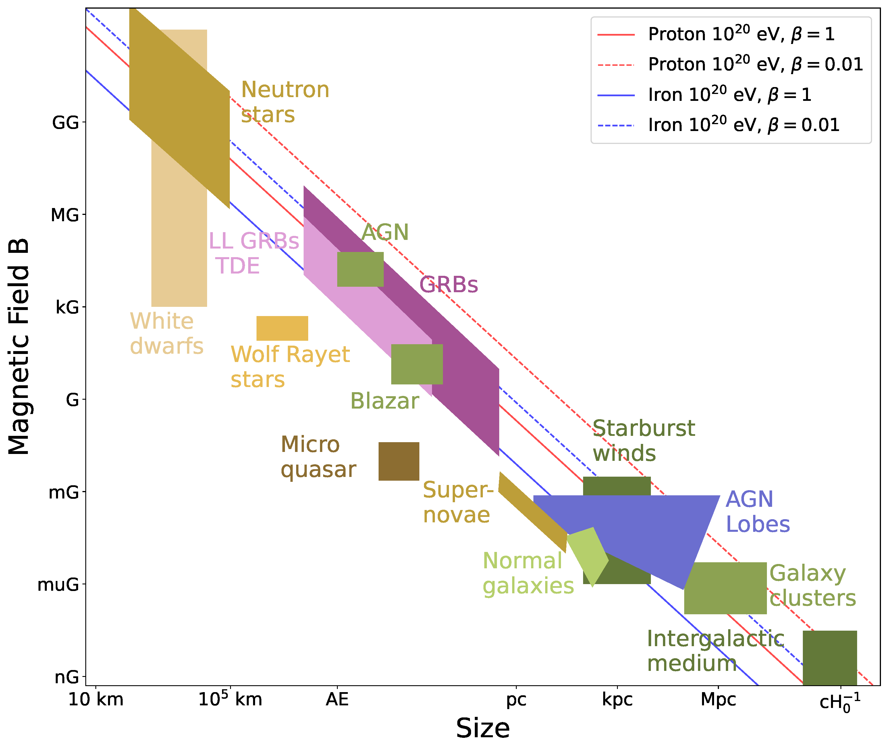
6.2. Anisotropy, Composition, and Time-Averaged Output
The observational evidence on the UHECR side is, correspondingly, statistical and directional rather than temporal. The Pierre Auger Observatory has established a large-scale dipole anisotropy in the arrival directions of cosmic rays above eV at more than , pointing away from the Galactic Center and thereby confirming an extragalactic origin [49]. On intermediate angular scales, the joint Pierre Auger–Telescope Array working group reports an excess correlated with the distribution of nearby starburst galaxies [50], while the Auger analysis of Phase I data finds the same starburst correlation together with a weaker signal when the catalog of -ray-bright AGN is used instead [51]. Blazars remain in the discussion both through these jetted-AGN correlations and through the recent, tentative association of the extreme Amaterasu event with a blazar under specific assumptions about its propagation and deflection [52,53]. The mass composition inferred by Auger, which becomes progressively heavier toward the highest energies, further shapes the interpretation, because heavier nuclei are deflected more strongly and are more easily accelerated to a given total energy through the rigidity dependence of the Hillas limit [49]. In every one of these arguments, the properties that determine whether a particular blazar could be a source, its magnetic field, its size, its Doppler factor, and hence its maximum rigidity and time-averaged particle output, are the properties that its variability constrains, which is why a time-domain understanding of the source population is a prerequisite for interpreting the anisotropy data even though the cosmic rays themselves carry no usable time information.
It is worth setting out the observational situation in more detail, because the composition data in particular shape which sources remain viable. The Auger dipole above eV has an amplitude of roughly and points about from the Galactic Center, firmly establishing the extragalactic origin of the highest-energy particles [49]. At higher energies, above ∼39 EeV, Auger reports an excess correlated with the flux pattern of nearby starburst galaxies at the ∼ level, together with a weaker signal associated with -ray-bright AGN [140], while the Telescope Array has reported an intermediate-scale “hotspot” in the northern sky that contains prominent HSP blazars such as Mrk 421 [141]. The interpretation of all these signals is entangled with composition: the depth-of-shower-maximum measurements from Auger indicate a progressive shift toward heavier nuclei above a few EeV, and because heavier nuclei of charge Z are deflected Z times more strongly by intervening magnetic fields, a mixed or heavy composition washes out the point-source correlations that a pure-proton flux would preserve [142]. This composition–deflection degeneracy is the central obstacle to identifying individual UHECR sources, and it is precisely why the mass-resolved measurements promised by the AugerPrime upgrade are so important. The through-line for this review is that the source parameters entering every one of these interpretations, maximum rigidity, jet power, escape efficiency, and time-averaged luminosity, are quantities constrained by the source’s electromagnetic variability, even though the cosmic rays themselves arrive with all their own timing information erased [45,135].
7. Prospects for Time-Domain Multi-Messenger Astronomy
The coming decade will transform the time-domain, multi-messenger study of blazars through the near-simultaneous arrival of several major facilities, each of which addresses a different link in the chain developed in this review. Realizing their combined potential depends on treating variability, across all messengers, as the connective tissue of the analysis.
7.1. Next-Generation Facilities
In the VHE band, the Cherenkov Telescope Array Observatory (CTAO) will improve flux sensitivity by roughly an order of magnitude over current instruments and, crucially for this review, will resolve variability on sub-hour timescales across a wide energy range, allowing the fastest flares to be characterized spectrally rather than merely detected [143]. Table 4 previews these facilities, the capability gain each brings, and its specific role in the time-domain programme developed in this review, before each is discussed in turn. Its low-energy threshold overlaps with the Fermi-LAT band, providing seamless coverage across the GeV–TeV transition where leptonic and hadronic models diverge most sharply. Complementing CTAO’s pointed, high-sensitivity observations, the Southern Wide-field Gamma-ray Observatory (SWGO), a wide-field, ground-level particle array now moving from its development phase toward construction, with its site selected at Pampa La Bola in the Atacama Astronomical Park, Chile (4770 m a.s.l.), will provide unbiased, continuous monitoring of the southern VHE sky with a duty cycle near unity, from a few hundred GeV into the PeV domain [144,145]. This continuous coverage catches the rare and unpredictable extreme flares that pointed instruments miss and enables genuine long-term VHE light curves; deployment is staged, beginning with a Pathfinder and the first science-capable array SWGO-A, and its southern location and proximity to CTAO make the two facilities strongly complementary [145]. In the neutrino sector, IceCube-Gen2 will increase the effective volume roughly eight-fold and improve point-source sensitivity by about a factor of five, and, most relevant here, it will lower the real-time alert threshold and raise the alert rate substantially, making prompt multi-wavelength follow-up of neutrino events routine rather than exceptional [146]. On the cosmic-ray side, the AugerPrime upgrade, commissioned in 2024 and now operating as a full multi-hybrid observatory, delivers event-by-event mass composition, sharpening the anisotropy analyzes whose interpretation, as argued in Section 6, depends on the composition-driven magnetic deflection [147,148]. Its Phase II surface array is expected to operate for at least a decade, until 2035 or beyond, accumulating a mass-resolved data set at the highest energies [148].
Alongside these large observatories, smaller dedicated arrays contribute in a way that bears specifically on the composition inference discussed in Section 6. The Horizon-T system at the Tien Shan high-altitude station, with ten detection points spread over ∼ km and a timing resolution of order nanoseconds, is designed to resolve the temporal structure of individual showers above eV rather than to accumulate exposure, and has reported events whose particles arrive in several distinct disks rather than the single front predicted by the standard nuclear-electromagnetic cascade [149]. The DUCK system, now being built with comparable timing resolution, is intended to provide an independent check on those observations [150]. Whatever the eventual interpretation of such events, the relevance here is methodological: the conversion of shower observables into a primary mass, on which the composition–deflection degeneracy of Section 6 entirely depends, rests on hadronic interaction models extrapolated well beyond accelerator energies, and detailed measurements of individual shower development are one of the few ways to test those models directly. Small, high-time-resolution arrays are therefore complementary to the large-exposure observatories in a specific sense: the latter measure the composition, the former help calibrate what a composition measurement means.
Table 4.
Next-generation multi-messenger facilities relevant to the time-domain study of blazars as particle accelerators. For each instrument we list the messenger and energy band it probes, its principal capability gain over current facilities, and the specific role it plays in the variability-based programme developed in this review. Sensitivity figures are approximate and design-dependent.
Each of these facilities also contributes a distinct piece of the puzzle beyond raw sensitivity. In the neutrino sector, the diffuse astrophysical flux first established by IceCube in 2013 set the energy scale that all source models must reproduce, and the transition now underway is from measuring that diffuse flux to resolving the individual sources within it, a transition that depends on the improved angular resolution and effective area of the next-generation detectors [146,153].
X-ray polarimetry has emerged as an unexpectedly powerful discriminant. The finding by IXPE that the X-ray polarization degree of HSP blazars such as Mrk 501 exceeds the optical degree points to an energy-stratified shock-acceleration geometry, in which the highest-energy particles occupy the most ordered part of the field, and monitoring the polarization angle through a flare tests whether the field is steady or reconfiguring [151,152]. The most constraining single result so far comes from BL Lacertae, observed by IXPE in November 2023 during the brightest millimeter outburst recorded from the source in four decades: the optical polarization degree reached a historical maximum of ∼ while no X-ray polarization was detected, giving a upper limit of [154]. The contrast is what carries the weight. Hadronic processes, whether proton synchrotron or pair synchrotron, generically predict X-ray polarization comparable to that of the radio and optical synchrotron emission, and this expectation survives in multi-zone geometries; leptonic inverse-Compton scattering, by contrast, depolarizes. A high optical degree together with a stringent X-ray upper limit therefore disfavors a hadronic origin for the X-rays in this source, and subsequent modeling of the full polarization SED finds that neither purely hadronic nor hybrid solutions satisfy the X-ray constraint [155]. The conclusion is not airtight: the same observations have since been reproduced by a proton-synchrotron model in which adiabatic rather than radiative losses set the cooling time, so that the intrinsic polarization is low and the variability timescale short [156]. What the episode establishes beyond dispute is the method. A single polarimetric non-detection, paired with a simultaneous optical measurement, constrained the emission mechanism more sharply than years of SED fitting had managed, and it did so because the two measurements are independent.
Two developments will extend this reach into the band where the hadronic signature is predicted to sit. The Compton Spectrometer and Imager (COSI) will survey the MeV sky with polarization sensitivity and a wide field of view [157]. Both properties matter here: the MeV band is where the electromagnetic cascade accompanying and Bethe–Heitler interactions deposits its energy, as set out in Section 3, and a wide field means hadronic flares can be caught as they happen rather than only when a pointed instrument is already looking, which is the same argument that makes SWGO complementary to CTAO. Further ahead, the proposed AMEGO-X and AMEGO concepts would improve MeV continuum sensitivity by a further order of magnitude, closing the “MeV gap” and turning the X-ray cascade constraint of Equation (6) from an upper limit into a measurement [158,159].
This polarimetric and MeV time-domain information is complementary to the flux light curves and, crucially, discriminates hadronic from leptonic scenarios through the degree of polarization and the stability of the polarization angle during neutrino-active states, as noted in Section 2. The combination of these facilities therefore does not merely add sensitivity in separate channels; it closes the loop between the electromagnetic variability, the polarization, the neutrino timing, and the cosmic-ray composition that this review has argued are all facets of the same accelerator.
7.2. Coordinated Real-Time Multi-Messenger Campaigns
The scientific return of these facilities is maximized not in isolation but through coordinated, real-time campaigns. The archetypal “golden event” would combine an IceCube-Gen2 neutrino alert, a prompt CTAO measurement of the simultaneous TeV spectrum and its sub-hour variability, IXPE X-ray polarimetry constraining the magnetic-field geometry, and continuous SWGO and Fermi-LAT coverage establishing the broadband flaring state, all triggered within hours of the neutrino arrival. Such a campaign would test, in a single source and a single flare, whether the neutrino is co-produced with the VHE photons in one compact zone or arises from a decoupled region, whether the polarization signals ordered or turbulent fields, and whether the inferred parameters place the source above the UHECR acceleration threshold. The time-domain infrastructure to make these connections, low-latency alerts, rapid-slewing instruments, and the statistical frameworks to correlate multi-messenger light curves against a red-noise background, is as essential to the enterprise as the sensitivity of any individual detector.
8. Summary and Conclusions
This review has advanced a single organizing thesis: blazar variability is not a complication to be averaged away but the primary diagnostic of how these sources accelerate particles to the highest energies. Read through this lens, an otherwise sprawling field collapses onto one principle, the amplitude, timescale, spectral evolution, inter-band correlation, and polarization behavior of the variability each constrain a specific physical property of the accelerator, and it is the temporal behavior, not the time-averaged spectrum, that breaks the persistent degeneracy between leptonic and lepto-hadronic emission scenarios. The three variability regimes of Table 1, the two model families of Table 2, and the benchmark sources of Table 3 are all facets of this one idea, and the chain of relations from the causality bound of Equation (2) to the Hillas criterion of Equation (9) is its quantitative backbone.
Four conclusions follow. First, rapid variability is the most powerful single constraint on the emission region. Minute-scale flares in the GeV and TeV bands force compact, high-Doppler-factor, high-field zones through the joint action of the causality bound, Equation (2), and the -transparency requirement, Equation (3); these are precisely the quantities R, , and B that enter the Hillas criterion, Equation (9), and therefore determine whether a source can reach ultra-high energies. The “Doppler-factor crisis” of the fastest TeV flares is not a peripheral curiosity but a direct, quantitative window onto the smallest and most extreme acceleration sites in the jet. Second, the multi-messenger connection is fundamentally a problem of timing, and the three messengers must be treated according to the temporal information they carry. Neutrinos preserve the correlation with electromagnetic flares and can be tied to specific variability states, as the two faces of the TXS 0506+056 story, the 2017 flaring coincidence and the 2014–2015 orphan excess, together demonstrate, while the fixed pion branching of Equation (5) and the efficiency relation of Equation (6) make the neutrino output a quantitative, testable corollary of hadronic -ray production. Charged cosmic rays, by contrast, lose all timing information to the magnetic delays of Equations (7) and (8), which reach millions of years for heavy nuclei and can therefore be associated with sources only through directional, time-averaged arguments. Third, the VHE band ties these threads together, both because it hosts the fastest variability and because the contrast between rapidly varying primary emission and steady, propagation-induced secondary emission offers an independent, purely temporal handle on the hadronic content of the jet. Fourth, and cutting across all of these, polarization, particularly the X-ray polarization now accessible with IXPE, adds a largely independent time-domain axis whose stability or rotation during a neutrino-active state may prove the cleanest single discriminant between leptonic and hadronic scenarios.
These conclusions are drawn against a backdrop of genuine and unresolved tensions, and intellectual honesty requires stating them plainly. The compactness demanded by the fastest flares remains in stark tension with the jet sizes inferred from radio imaging, and no structured-jet model, minijets, spine-sheath, or turbulence, yet accounts for the full phenomenology without introducing parameters that are themselves poorly constrained. Single-zone lepto-hadronic fits to the most compelling neutrino–blazar candidate, TXS 0506+056, an association at only ∼ and therefore suggestive rather than established, require proton luminosities that strain or exceed the Eddington limit and tend to overproduce the observed X-rays, so that even the flagship case is not comfortably explained. The stacking limits show that the resolved -ray blazar population accounts for at most a fraction of the diffuse neutrino flux, implying that efficient neutrino production is confined to particular sources or particular states rather than being generic. And on the cosmic-ray side, the drift toward heavy composition at the highest energies entangles source identification with magnetic deflection in a way that current data cannot disentangle. None of these tensions is fatal to the blazar hypothesis, but each is a reminder that the case remains circumstantial and that variability, powerful as it is, constrains rather than confirms.
The next decade is positioned to resolve much of this ambiguity, because for the first time the relevant facilities will operate contemporaneously and can be coordinated in real time. CTAO will resolve sub-hour VHE variability with an order-of-magnitude sensitivity gain; SWGO will provide the continuous, unbiased southern-sky monitoring that catches the rare extreme flares; IceCube-Gen2 will lower the neutrino alert threshold and raise the alert rate enough to make prompt multi-wavelength follow-up routine; and AugerPrime will deliver the event-by-event composition needed to interpret the anisotropy data. The scientific payoff lies not in any one of these instruments but in their coordination: the archetypal “golden event”, a neutrino alert followed within hours by a resolved TeV spectrum and its sub-hour variability, by X-ray polarimetry constraining the field geometry, and by broadband light curves establishing the flaring state, would test, in a single source and a single flare, whether the neutrino is co-produced with the VHE photons in one compact zone or arises from a decoupled region, whether the field is ordered or turbulent, and whether the inferred parameters place the source above the acceleration threshold of Equation (9).
The broader significance of this program extends beyond blazars. The question of where the most energetic particles in the Universe originate has remained open since the discovery of ultra-high-energy cosmic rays, and blazars are among the few candidate accelerators that satisfy the Hillas criterion while being numerous, nearby, and observable across every messenger. If they are indeed the sources, the identification will not come from a single spectrum or a single arrival direction; it will come from the time domain, from the coordinated recognition of the same accelerator flaring simultaneously in photons and neutrinos, with its polarization and its inferred parameters all pointing the same way. The central message of this review is therefore both methodological and physical: understanding blazars, and through them, the origin of the highest-energy cosmic rays and neutrinos, requires understanding not merely what these sources look like, but how, and how fast, they change.
Funding
This research was funded by the Fundação de Amparo à Pesquisa do Estado de São Paulo (FAPESP), via grant numbers 2021/01089-1, 2024/02267-9, and 2024/14769-9, and by the Conselho Nacional de Desenvolvimento Científico e Tecnológico (CNPq), grant numbers 403337/2024-0, 153839/2024-4, and 200164/2025-2.
Data Availability Statement
No new data were created or analyzed in this study. Data sharing is not applicable to this article.
Acknowledgments
During the preparation of this manuscript, the author used Claude (Anthropic; model Sonnet 5) to assist in generating the schematic Figure 1, Figure 3, Figure 4 and Figure 5, Figure 6 and Figure 8. For these figures, the tool was used to produce the LaTeX (TikZ/pgfplots) drawing code from the layout, physical content, functional forms, and parameter values specified by the author; it was not used to generate, analyze, or fit any data. The author has reviewed and edited the output and takes full responsibility for the scientific content and accuracy of all figures and of this publication.
Conflicts of Interest
The author declares no conflicts of interest.
Abbreviations
The following abbreviations are used in this manuscript:
| AGN | Active Galactic Nucleus/Nuclei |
| ASAS-SN | All-Sky Automated Survey for Supernovae |
| BL Lac | BL Lacertae object |
| BLR | Broad Line Region |
| CARMA | Continuous-time Autoregressive Moving Average |
| CTAO | Cherenkov Telescope Array Observatory |
| EBL | Extragalactic Background Light |
| EC | External Compton |
| EHSP | Extreme High-Synchrotron-Peaked |
| FSRQ | Flat-Spectrum Radio Quasar |
| H.E.S.S. | High Energy Stereoscopic System |
| HSP | High-Synchrotron-Peaked |
| IACT | Imaging Atmospheric Cherenkov Telescope |
| IDV | Intraday Variability |
| IGMF | Intergalactic Magnetic Field |
| ISP | Intermediate-Synchrotron-Peaked |
| IXPE | Imaging X-ray Polarimetry Explorer |
| KVA | Kungliga Vetenskapsakademien (telescope) |
| LAT | Large Area Telescope (Fermi) |
| LSP | Low-Synchrotron-Peaked |
| LST | Large-Sized Telescope (CTAO) |
| MAGIC | Major Atmospheric Gamma-ray Imaging Cherenkov (telescopes) |
| MCMC | Markov Chain Monte Carlo |
| NuSTAR | Nuclear Spectroscopic Telescope Array |
| OVRO | Owens Valley Radio Observatory |
| PSD | Power Spectral Density |
| REM | Rapid Eye Mount (telescope) |
| SED | Spectral Energy Distribution |
| SSC | Synchrotron Self-Compton |
| SWGO | Southern Wide-field Gamma-ray Observatory |
| TESS | Transiting Exoplanet Survey Satellite |
| UHECR | Ultra-High-Energy Cosmic Ray |
| UVOT | Ultraviolet/Optical Telescope (Swift) |
| VERITAS | Very Energetic Radiation Imaging Telescope Array System |
| VHE | Very High Energy ( GeV) |
| VLBI | Very Long Baseline Interferometry |
| WEBT | Whole Earth Blazar Telescope |
| XRT | X-Ray Telescope (Swift) |
References
- Blandford, R.D.; Znajek, R.L. Electromagnetic extraction of energy from Kerr black holes. Mon. Not. R. Astron. Soc. 1977, 179, 433–456. [Google Scholar] [CrossRef] [Scilit]
- Blandford, R.D.; Payne, D.G. Hydromagnetic flows from accretion disks and the production of radio jets. Mon. Not. R. Astron. Soc. 1982, 199, 883–903. [Google Scholar] [CrossRef] [Scilit]
- Blandford, R.; Meier, D.; Readhead, A. Relativistic Jets from Active Galactic Nuclei. Annu. Rev. Astron. Astrophys. 2019, 57, 467–509. [Google Scholar] [CrossRef] [Scilit]
- Sikora, M.; Madejski, G. On pair content and variability of sub-parsec jets in quasars. Astrophys. J. 2000, 534, 109. [Google Scholar] [CrossRef] [Scilit]
- Urry, C.M.; Padovani, P. Unified Schemes for Radio-Loud Active Galactic Nuclei. Publ. Astron. Soc. Pac. 1995, 107, 803. [Google Scholar] [CrossRef] [Scilit] [PubMed]
- Wagner, S.J.; Witzel, A. Intraday Variability In Quasars and BL Lac Objects. Annu. Rev. Astron. Astrophys. 1995, 33, 163–198. [Google Scholar] [CrossRef]
- Falomo, R.; Pian, E.; Treves, A. An optical view of BL Lacertae objects. Astron. Astrophys. Rev. 2014, 22, 73. [Google Scholar] [CrossRef] [Scilit]
- Madejski, G.G.; Sikora, M. Gamma-Ray Observations of Active Galactic Nuclei. Annu. Rev. Astron. Astrophys. 2016, 54, 725–760. [Google Scholar] [CrossRef] [Scilit]
- Webb, J.R. 30 Years of Multifrequency Quasar Variability: A Personal Journey. Galaxies 2021, 9, 69. [Google Scholar] [CrossRef] [Scilit]
- Aharonian, F.; Akhperjanian, A.G.; Bazer-Bachi, A.R.; Behera, B.; Beilicke, M.; Benbow, W.; Berge, D.; Bernlöhr, K.; Boisson, C.; Bolz, O. An Exceptional Very High Energy Gamma-Ray Flare of PKS 2155-304. Astrophys. J. Lett. 2007, 664, L71–L78. [Google Scholar] [CrossRef] [Scilit]
- Begelman, M.C.; Fabian, A.C.; Rees, M.J. Implications of very rapid TeV variability in blazars. Mon. Not. R. Astron. Soc. 2008, 384, 19. [Google Scholar] [CrossRef] [Scilit]
- Pandey, A.; Stalin, C.S. Detection of minute-timescale γ-ray variability in BL Lacertae by Fermi-LAT. Astron. Astrophys. 2022, 668, A152. [Google Scholar] [CrossRef] [Scilit]
- Abe, K.; Abe, S.; Abhishek, A.; Acero, F.; Aguasca-Cabot, A.; Agudo, I.; Alispach, C.; Ambrosino, D.; Ambrosino, F.; Antonelli, L.A.; et al. Very-high-energy gamma-ray intranight variability from BL Lacertae during the extreme flaring state of 2022. Astron. Astrophys. 2026, 710, A41. [Google Scholar] [CrossRef] [Scilit]
- Albert, J.; Aliu, E.; Anderhub, H.; Antoranz, P.; Armada, A.; Baixeras, C.; Barrio, J.A.; Bartko, H.; Bastieri, D.; Becker, J.K. Variable VHE gamma-ray emission from Markarian 501. Astrophys. J. 2007, 669, 862–883. [Google Scholar] [CrossRef] [Scilit] [PubMed]
- Otero-Santos, J.; Raiteri, C.M.; Acosta-Pulido, J.A.; Carnerero, M.I.; Villata, M.; Savchenko, S.S.; Carosati, D.; Chen, W.P.; Kurtanidze, S.O.; Joner, M.D.; et al. Optical variability of the blazar 3C 371: From minute to year timescales. Astron. Astrophys. 2024, 686, A228. [Google Scholar] [CrossRef] [Scilit]
- Pandey, A.; Bachev, R.; Czerny, B.; Wiita, P.J.; Gupta, A.C.; Strigachev, A.; Popowicz, A. Investigating the origin of optical flares from the TeV blazar S4 0954+65. Astron. Astrophys. 2023, 679, A28. [Google Scholar] [CrossRef] [Scilit]
- Miller, H.R.; Carini, M.T.; Goodrich, B.D. Detection of microvariability for BL Lacertae objects. Nature 1989, 337, 627. [Google Scholar] [CrossRef] [Scilit]
- Gupta, A.C.; Agarwal, A.; Bhagwan, J.; Strigachev, A.; Bachev, R.; Semkov, E.; Gaur, H.; Damljanovic, G.; Vince, O.; Wiita, P.J. Multiband optical variability of three TeV blazars on diverse time-scales. Mon. Not. R. Astron. Soc. 2016, 458, 1127–1137. [Google Scholar] [CrossRef] [Scilit]
- Kirk, J.G.; Rieger, F.M.; Mastichiadis, A. Particle acceleration and synchrotron emission in blazar jets. arXiv 1998, arXiv:astro-ph/9801265. [Google Scholar] [CrossRef] [Scilit]
- Zhang, Y.H.; Treves, A.; Celotti, A.; Chiappetti, L.; Fossati, G.; Ghisellini, G.; Maraschi, L.; Pian, E.; Tagliaferri, G.; Tavecchio, F. Four years monitoring of blazar pks 2155-304 with bepposax: Probing the dynamics of the jet. Astrophys. J. 2002, 572, 762. [Google Scholar] [CrossRef] [Scilit] [PubMed]
- Ackermann, M.; Ajello, M.; Albert, A.; Atwood, W.B.; Baldini, L.; Ballet, J.; Barbiellini, G.; Bastieri, D.; Gonzalez, J.B.; Bellazzini, R. Multiwavelength Evidence for Quasi-periodic Modulation in the Gamma-Ray Blazar PG 1553+113. Astrophys. J. Lett. 2015, 813, L41. [Google Scholar] [CrossRef] [Scilit]
- Bhatta, G.; Zola, S.; Stawarz, Ł.; Ostrowski, M.; Winiarski, M.; Ogłoza, W.; Dróżdż, M.; Siwak, M.; Liakos, A.; Kozieł-Wierzbowska, D. Detection of Possible Quasi-periodic Oscillations in the Long-term Optical Light Curve of the BL Lac Object OJ 287. Astrophys. J. 2016, 832, 47. [Google Scholar] [CrossRef] [Scilit]
- Raiteri, C.M.; Villata, M.; Larionov, V.M.; Jorstad, S.G.; Marscher, A.P.; Weaver, Z.R.; Acosta-Pulido, J.A.; Agudo, I.; Andreeva, T.; Arkharov, A.; et al. The complex variability of blazars: Time-scales and periodicity analysis in S4 0954+65. Mon. Not. R. Astron. Soc. 2021, 504, 5629–5646. [Google Scholar] [CrossRef] [Scilit]
- Maraschi, L.; Ghisellini, G.; Celotti, A. A jet model for the gamma-ray emitting blazar 3C 279. Astrophys. J. Lett. 1992, 397, L5–L9. [Google Scholar] [CrossRef] [Scilit] [PubMed]
- Sikora, M.; Begelman, M.C.; Rees, M.J. Comptonization of Diffuse Ambient Radiation by a Relativistic Jet: The Source of Gamma Rays from Blazars? ApJ 1994, 421, 153. [Google Scholar] [CrossRef] [Scilit] [PubMed]
- Ghisellini, G.; Celotti, A.; Fossati, G.; Maraschi, L.; Comastri, A. A Theoretical unifying scheme for gamma-ray bright blazars. Mon. Not. R. Astron. Soc. 1998, 301, 451. [Google Scholar] [CrossRef] [Scilit]
- Mannheim, K. The proton blazar. arXiv 1993, arXiv:astro-ph/9302006. [Google Scholar] [CrossRef] [Scilit]
- Mücke, A.; Protheroe, R.J.; Engel, R.; Rachen, J.P.; Stanev, T. BL Lac Objects in the synchrotron proton blazar model. Astropart. Phys. 2003, 18, 593–613. [Google Scholar] [CrossRef] [Scilit]
- Böttcher, M.; Reimer, A.; Sweeney, K.; Prakash, A. Leptonic and Hadronic Modeling of Fermi-Detected Blazars. Astrophys. J. 2013, 768, 54. [Google Scholar] [CrossRef] [Scilit]
- Cerruti, M.; Zech, A.; Boisson, C.; Inoue, S. A hadronic origin for ultra-high-frequency-peaked BL Lac objects. Mon. Not. R. Astron. Soc. 2015, 448, 910–927. [Google Scholar] [CrossRef] [Scilit]
- Atoyan, A.; Dermer, C.D. High-Energy Neutrinos from Photomeson Processes in Blazars. Phys. Rev. Lett. 2001, 87, 221102. [Google Scholar] [CrossRef] [Scilit] [PubMed]
- Murase, K.; Inoue, Y.; Dermer, C.D. Diffuse Neutrino Intensity from the Inner Jets of Active Galactic Nuclei: Impacts of External Photon Fields and the Blazar Sequence. Phys. Rev. D 2014, 90, 023007. [Google Scholar] [CrossRef] [Scilit]
- Rodrigues, X.; Heinze, J.; Palladino, A.; Van Vliet, A.; Winter, W. Active Galactic Nuclei Jets as the Origin of Ultrahigh-Energy Cosmic Rays and Perspectives for the Detection of Astrophysical Source Neutrinos at EeV Energies. Phys. Rev. Lett. 2021, 126, 191101. [Google Scholar] [CrossRef] [Scilit] [PubMed]
- Krawczynski, H.; Hughes, S.B.; Horan, D.; Aharonian, F.; Aller, M.F.; Aller, H.; Boltwood, P.; Buckley, J.; Coppi, P.; Fossati, G. Multiwavelength Observations of Strong Flares from the TeV Blazar 1ES 1959+650. Astrophys. J. 2004, 601, 151–164. [Google Scholar] [CrossRef] [Scilit] [PubMed]
- Böttcher, M. A Hadronic Synchrotron Mirror Model for the “Orphan” TeV Flare in 1ES 1959+650. Astrophys. J. 2005, 621, 176–180, Erratum in Astrophys. J. 2006, 641, 1233. [Google Scholar] [CrossRef] [Scilit] [PubMed]
- MacDonald, N.R.; Marscher, A.P.; Jorstad, S.G.; Joshi, M. Through the Ring of Fire: γ-ray Variability in Blazars by a Moving Plasmoid Passing a Local Source of Seed Photons. Astrophys. J. 2015, 804, 111. [Google Scholar] [CrossRef] [Scilit]
- Zhang, H.; Böttcher, M. X-Ray and Gamma-Ray Polarization in Leptonic and Hadronic Jet Models of Blazars. Astrophys. J. 2013, 774, 18. [Google Scholar] [CrossRef] [Scilit]
- Liodakis, I.; Marscher, A.P.; Agudo, I.; Berdyugin, A.V.; Bernardos, M.I.; Bonnoli, G.; Borman, G.A.; Casadio, C.; Casanova, V.; Cavazzuti, E.; et al. Polarized blazar X-rays imply particle acceleration in shocks. Nature 2022, 611, 677–681. [Google Scholar] [CrossRef] [Scilit] [PubMed]
- Aartsen, M.G. et al. [IceCube Collaboration] Multimessenger observations of a flaring blazar coincident with high-energy neutrino IceCube-170922A. Science 2018, 361, eaat1378. [Google Scholar] [CrossRef] [Scilit] [PubMed]
- Aartsen, M.G. et al. [IceCube Collaboration] Neutrino emission from the direction of the blazar TXS 0506+056 prior to the IceCube-170922A alert. Science 2018, 361, 147–151. [Google Scholar] [CrossRef] [Scilit] [PubMed]
- Cerruti, M.; Zech, A.; Boisson, C.; Emery, G.; Inoue, S.; Lenain, J.P. Leptohadronic single-zone models for the electromagnetic and neutrino emission of TXS 0506+056. Mon. Not. R. Astron. Soc. 2019, 483, L12–L16, Correction in Mon. Not. R. Astron. Soc. 2021, 502, L21–L22. [Google Scholar] [CrossRef] [Scilit]
- Gao, S.; Fedynitch, A.; Winter, W.; Pohl, M. Modelling the coincident observation of a high-energy neutrino and a bright blazar flare. Nat. Astron. 2019, 3, 88–92. [Google Scholar] [CrossRef] [Scilit]
- Petropoulou, M.; Murase, K.; Santander, M.; Buson, S.; Tohuvavohu, A.; Kawamuro, T.; Vasilopoulos, G.; Negoro, H.; Ueda, Y.; Siegel, M.H.; et al. Multi-Epoch Modeling of TXS 0506+056 and Implications for Long-Term High-Energy Neutrino Emission. Astrophys. J. 2020, 891, 115. [Google Scholar] [CrossRef] [Scilit]
- Waxman, E.; Miralda-Escude, J. Images of bursting sources of high-energy cosmic rays. 1. Effects of magnetic fields. Astrophys. J. Lett. 1996, 472, L89–L92. [Google Scholar] [CrossRef] [Scilit]
- Kotera, K.; Olinto, A.V. The Astrophysics of Ultrahigh-Energy Cosmic Rays. Annu. Rev. Astron. Astrophys. 2011, 49, 119–153. [Google Scholar] [CrossRef] [Scilit]
- Hillas, A.M. The Origin of Ultra-High-Energy Cosmic Rays. Annu. Rev. Astron. Astrophys. 1984, 22, 425–444. [Google Scholar] [CrossRef]
- Murase, K.; Dermer, C.D.; Takami, H.; Migliori, G. Blazars as Ultra-high-energy Cosmic-ray Sources: Implications for TeV Gamma-Ray Observations. Astrophys. J. 2012, 749, 63. [Google Scholar] [CrossRef] [Scilit]
- Matthews, J.H.; Bell, A.R.; Blundell, K.M.; Araudo, A.T. Ultrahigh energy cosmic rays from shocks in the lobes of powerful radio galaxies. Mon. Not. R. Astron. Soc. 2019, 482, 4303–4321. [Google Scholar] [CrossRef] [Scilit]
- Aab, A. et al. [The Pierre Auger Collaboration] Observation of a Large-scale Anisotropy in the Arrival Directions of Cosmic Rays above 8 × 10¹⁸ eV. Science 2017, 357, 1266–1270. [Google Scholar] [CrossRef] [Scilit] [PubMed]
- di Matteo, A.; Anchordoqui, L.A.; Bister, T.; Biteau, J.; Caccianiga, L.; de Almeida, R.M.; Deligny, O.; Giaccari, U.; Harari, D.; Kim, J.; et al. UHECR arrival directions in the latest data from the original Auger and TA surface detectors and nearby galaxies. PoS 2021, ICRC2021, 308. [Google Scholar] [CrossRef] [Scilit]
- Abreu, P.; Aglietta, M.; Albury, J.M.; Allekotte, I.; Cheminant, K.A.; Almela, A.; Alvarez-Muñiz, J.; Batista, R.A.; Yebra, J.A.; Anastasi, G.A.; et al. Arrival Directions of Cosmic Rays above 32 EeV from Phase One of the Pierre Auger Observatory. Astrophys. J. 2022, 935, 170. [Google Scholar] [CrossRef] [Scilit]
- Abbasi, R.U. et al. [Telescope Array Collaboration] An extremely energetic cosmic ray observed by a surface detector array. Science 2023, 382, abo5095. [Google Scholar] [CrossRef] [Scilit] [PubMed]
- Das, S.; Hazra, S.; Gupta, N. Cosmic Clues from Amaterasu: Blazar-driven Ultrahigh-energy Cosmic Rays? Astrophys. J. Lett. 2025, 988, L8. [Google Scholar] [CrossRef] [Scilit]
- Franceschini, A.; Rodighiero, G.; Vaccari, M. Extragalactic optical-infrared background radiation, its time evolution and the cosmic photon-photon opacity. Astron. Astrophys. 2008, 487, 837–852. [Google Scholar] [CrossRef] [Scilit]
- Domínguez, A.; Primack, J.R.; Rosario, D.J.; Prada, F.; Gilmore, R.C.; Faber, S.M.; Koo, D.C.; Somerville, R.S.; Pérez-Torres, M.A.; Pérez-González, P.; et al. Extragalactic background light inferred from AEGIS galaxy-SED-type fractions. Mon. Not. R. Astron. Soc. 2011, 410, 2556–2578. [Google Scholar] [CrossRef] [Scilit]
- Neronov, A.; Vovk, I. Evidence for strong extragalactic magnetic fields from Fermi observations of TeV blazars. Science 2010, 328, 73–75. [Google Scholar] [CrossRef] [Scilit] [PubMed]
- Biteau, J.; Prandini, E.; Costamante, L.; Lemoine, M.; Padovani, P.; Pueschel, E.; Resconi, E.; Tavecchio, F.; Taylor, A.; Zech, A. Progress in unveiling extreme particle acceleration in persistent astrophysical jets. Nat. Astron. 2020, 4, 124–131. [Google Scholar] [CrossRef] [Scilit]
- Essey, W.; Kalashev, O.E.; Kusenko, A.; Beacom, J.F. Secondary photons and neutrinos from cosmic rays produced by distant blazars. Phys. Rev. Lett. 2010, 104, 141102. [Google Scholar] [CrossRef] [Scilit] [PubMed]
- Takami, H.; Murase, K.; Dermer, C.D. Disentangling Hadronic and Leptonic Cascade Scenarios from the Very-High-Energy Gamma-Ray Emission of Distant Hard-Spectrum Blazars. Astrophys. J. Lett. 2013, 771, L32. [Google Scholar] [CrossRef] [Scilit]
- Fossati, G.; Maraschi, L.; Celotti, A.; Comastri, A.; Ghisellini, G. A Unifying view of the spectral energy distributions of blazars. Mon. Not. R. Astron. Soc. 1998, 299, 433–448. [Google Scholar] [CrossRef] [Scilit]
- Abdo, A.A.; Ackermann, M.; Agudo, I.; Ajello, M.; Aller, H.D.; Aller, M.F.; Angelakis, E.; Arkharov, A.A.; Axelsson, M.; Bach, U.; et al. The Spectral Energy Distribution of Fermi Bright Blazars. Astrophys. J. 2010, 716, 30–70. [Google Scholar] [CrossRef] [Scilit]
- Ajello, M.; Angioni, R.; Axelsson, M.; Ballet, J.; Barbiellini, G.; Bastieri, D.; Gonzalez, J.B.; Bellazzini, R.; Bissaldi, E.; Bloom, E.D.; et al. The Fourth Catalog of Active Galactic Nuclei Detected by the Fermi Large Area Telescope. Astrophys. J. 2020, 892, 105. [Google Scholar] [CrossRef] [Scilit]
- Ghisellini, G.; Righi, C.; Costamante, L.; Tavecchio, F. The Fermi blazar sequence. Mon. Not. R. Astron. Soc. 2017, 469, 255–266. [Google Scholar] [CrossRef] [Scilit]
- Costamante, L.; Ghisellini, G.; Giommi, P.; Tagliaferri, G.; Celotti, A.; Chiaberge, M.; Fossati, G.; Maraschi, L.; Tavecchio, F.; Treves, A.; et al. Extreme synchrotron bl lac objects. Astron. Astrophys. 2001, 371, 512. [Google Scholar] [CrossRef] [Scilit]
- Rybicki, G.B.; Lightman, A.P. Radiative Processes in Astrophysics; John Wiley & Sons: Hoboken, NJ, USA, 1986. [Google Scholar]
- Tavecchio, F.; Maraschi, L.; Ghisellini, G. Constraints on the physical parameters of TeV blazars. Astrophys. J. 1998, 509, 608. [Google Scholar] [CrossRef] [Scilit] [PubMed]
- Bhatta, G.; Dhital, N. The Nature of γ-Ray Variability in Blazars. Astrophys. J. 2020, 891, 120. [Google Scholar] [CrossRef] [Scilit]
- Webb, J.R.; Arroyave, V.; Laurence, D.; Revesz, S.; Bhatta, G.; Hollingsworth, H.; Dhalla, S.; Howard, E.; Cioffi, M. The Nature of Micro-Variability in Blazars. Galaxies 2021, 9, 114. [Google Scholar] [CrossRef] [Scilit]
- Webb, J.R.; Garcia, C.; Irizarry, J.; Moreno, D.; Marscher, A.P. Turbulent Cell Interpretation of Micro-Variability of BL Lacertae: Polarization. Galaxies 2026, 14, 24. [Google Scholar] [CrossRef] [Scilit]
- Tan, H.B.; Liu, R.Y.; Böttcher, M. Revisiting the TeV flare of PKS 2155-304 in 2006. Mon. Not. R. Astron. Soc. 2024, 529, 903–915. [Google Scholar] [CrossRef] [Scilit]
- Giannios, D.; Uzdensky, D.A.; Begelman, M.C. Fast TeV variability in blazars: Jets in a jet. Mon. Not. R. Astron. Soc. 2009, 395, L29–L33. [Google Scholar] [CrossRef] [Scilit]
- Tanihata, C.; Urry, C.M.; Takahashi, T.; Kataoka, J.; Wagner, S.J.; Madejski, G.M.; Tashiro, M.; Kouda, M. Variability timescales of TeV blazars observed in the ASCA continuous long look X-ray monitoring. Astrophys. J. 2001, 563, 569–581. [Google Scholar] [CrossRef] [Scilit] [PubMed]
- Saito, S.; Stawarz, Ł.; Tanaka, Y.T.; Takahashi, T.; Madejski, G.; D’Ammando, F. Very Rapid High-Amplitude Gamma-ray Variability in Luminous Blazar PKS 1510-089 Studied with Fermi-LAT. Astrophys. J. Lett. 2013, 766, L11. [Google Scholar] [CrossRef] [Scilit]
- Aleksić, J.; Ansoldi, S.; Antonelli, L.A.; Antoranz, P.; Babic, A.; Bangale, P.; de Almeida, U.B.; Barrio, J.A.; González, J.B.; Bednarek, W.; et al. Unprecedented study of the broadband emission of Mrk 421 during flaring activity in March 2010. Astron. Astrophys. 2015, 578, A22. [Google Scholar] [CrossRef] [Scilit]
- Gupta, A.C. X-ray Flux and Spectral Variability of the TeV Blazars Mrk 421 and PKS 2155-304. Galaxies 2020, 8, 64. [Google Scholar] [CrossRef] [Scilit]
- Ahnen, M.L.; Ansoldi, S.; Antonelli, L.A.; Antoranz, P.; Babic, A.; Banerjee, B.; Bangale, P.; de Almeida, U.B.; Barrio, J.A.; González, J.B.; et al. Multiband variability studies and novel broadband SED modeling of Mrk 501 in 2009. Astron. Astrophys. 2017, 603, A31. [Google Scholar] [CrossRef] [Scilit]
- Abdo, A.A.; Ackermann, M.; Ajello, M.; Antolini, E.; Baldini, L.; Ballet, J.; Barbiellini, G.; Bastieri, D.; Bechtol, K.; Bellazzini, R.; et al. Gamma-ray Light Curves and Variability of Bright Fermi-detected Blazars. Astrophys. J. 2010, 722, 520–542. [Google Scholar] [CrossRef] [Scilit]
- Ryan, J.L.; Siemiginowska, A.; Sobolewska, M.A.; Grindlay, J. Characteristic Variability Timescales in the Gamma-Ray Power Spectra of Blazars. Astrophys. J. 2019, 885, 12. [Google Scholar] [CrossRef] [Scilit]
- Emmanoulopoulos, D.; McHardy, I.M.; Papadakis, I.E. Generating artificial light curves: Revisited and updated. Mon. Not. R. Astron. Soc. 2013, 433, 907. [Google Scholar] [CrossRef] [Scilit]
- Jorstad, S.G.; Marscher, A.P.; Raiteri, C.M.; Villata, M.; Weaver, Z.R.; Zhang, H.; Dong, L.; Gómez, J.L.; Perel, M.V.; Savchenko, S.S.; et al. Rapid quasi-periodic oscillations in the relativistic jet of BL Lacertae. Nature 2022, 609, 265–268. [Google Scholar] [CrossRef] [Scilit] [PubMed]
- Peñil, P.; Domínguez, A.; Buson, S.; Ajello, M.; Otero-Santos, J.; Barrio, J.A.; Nemmen, R.; Cutini, S.; Rani, B.; Franckowiak, A.; et al. Systematic Search for γ-Ray Periodicity in Active Galactic Nuclei Detected by the Fermi Large Area Telescope. Astrophys. J. 2020, 896, 134. [Google Scholar] [CrossRef] [Scilit]
- Raiteri, C.M.; Villata, M. Blazar spectral variability as explained by a twisting inhomogeneous jet. Nature 2017, 552, 374–377. [Google Scholar] [CrossRef] [Scilit] [PubMed]
- Blinov, D.; Pavlidou, V.; Papadakis, I.; Kiehlmann, S.; Liodakis, I.; Panopoulou, G.V.; Angelakis, E.; Baloković, M.; Hovatta, T.; King, O.G.; et al. RoboPol: Connection between optical polarization plane rotations and gamma-ray flares in blazars. Mon. Not. R. Astron. Soc. 2018, 474, 1296–1306. [Google Scholar] [CrossRef] [Scilit]
- Gesu, L.D.; Marshall, H.L.; Ehlert, S.R.; Kim, D.E.; Donnarumma, I.; Tavecchio, F.; Liodakis, I.; Kiehlmann, S.; Agudo, I.; Jorstad, S.G.; et al. Discovery of X-ray polarization angle rotation in the jet from blazar Mrk 421. Nat. Astron. 2023, 7, 1245–1258. [Google Scholar] [CrossRef] [Scilit]
- Kim, D.E.; Di Gesu, L.; Liodakis, I.; Marscher, A.P.; Jorstad, S.G.; Middei, R.; Marshall, H.L.; Pacciani, L.; Agudo, I.; Tavecchio, F.; et al. Magnetic field properties inside the jet of Mrk 421. Multiwavelength polarimetry, including the Imaging X-ray Polarimetry Explorer. Astron. Astrophys. 2024, 681, A12. [Google Scholar] [CrossRef] [Scilit]
- Maksym, W.P.; Liodakis, I.; Saade, M.L.; Kim, D.E.; Middei, R.; Gesu, L.D.; Kiehlmann, S.; Matzeu, G.; Agudo, I.; Marscher, A.P.; et al. A Two-week IXPE Monitoring Campaign on Mrk 421. Astrophys. J. 2025, 986, 230. [Google Scholar] [CrossRef] [Scilit]
- Hu, X.K.; Yu, Y.W.; Zhang, J.; Wang, X.G.; Patra, K.C.; Brink, T.G.; Zheng, W.K.; Wang, Q.; Kong, D.F.; Chen, L.J.; et al. Multiwavelength Polarization Observations of Mrk 501. Astrophys. J. Lett. 2024, 970, L22. [Google Scholar] [CrossRef] [Scilit]
- Vaughan, S.; Edelson, R.; Warwick, R.S.; Uttley, P. On characterizing the variability properties of X-ray light curves from active galaxies. Mon. Not. R. Astron. Soc. 2003, 345, 1271–1284. [Google Scholar] [CrossRef] [Scilit]
- Dmytriiev, A.; Sol, H.; Zech, A. Connecting steady emission and very high energy flaring states in blazars: The case of Mrk 421. Mon. Not. R. Astron. Soc. 2021, 505, 2712–2730. [Google Scholar] [CrossRef] [Scilit]
- Bloom, S.D.; Marscher, A.P. An Analysis of the Synchrotron Self-Compton Model for the Multi–Wave Band Spectra of Blazars. Astrophys. J. 1996, 461, 657. [Google Scholar] [CrossRef] [Scilit]
- Dermer, C.D.; Schlickeiser, R. Model for the High-Energy Emission from Blazars. Astrophys. J. 1993, 416, 458. [Google Scholar] [CrossRef] [Scilit] [PubMed]
- Marscher, A.P.; Gear, W.K. Models for high-frequency radio outbursts in extragalactic sources, with application to the early 1983 millimeter-to-infrared flare of 3C 273. Astrophys. J. 1985, 298, 114–127. [Google Scholar] [CrossRef] [Scilit] [PubMed]
- Marscher, A.P.; Jorstad, S.G.; D’Arcangelo, F.D.; Smith, P.S.; Williams, G.G.; Larionov, V.M.; Oh, H.; Olmstead, A.R.; Aller, M.F.; Aller, H.D.; et al. The inner jet of an active galactic nucleus as revealed by a radio-to-γ-ray outburst. Nature 2008, 452, 966–969. [Google Scholar] [CrossRef] [Scilit] [PubMed]
- Marscher, A.P. Turbulent, Extreme Multi-Zone Model for Simulating Flux and Polarization Variability in Blazars. Astrophys. J. 2014, 780, 87. [Google Scholar] [CrossRef] [Scilit]
- Sironi, L.; Spitkovsky, A. Relativistic reconnection: An efficient source of non-thermal particles. Astrophys. J. Lett. 2014, 783, L21. [Google Scholar] [CrossRef] [Scilit]
- Petropoulou, M.; Giannios, D.; Sironi, L. Blazar flares powered by plasmoids in relativistic reconnection. Mon. Not. R. Astron. Soc. 2016, 462, 3325–3343. [Google Scholar] [CrossRef] [Scilit]
- Aharonian, F.A. TeV gamma-rays from BL Lac objects due to synchrotron radiation of extremely high-energy protons. New Astron. 2000, 5, 377–395. [Google Scholar] [CrossRef] [Scilit]
- Boettcher, M. Modeling the Emission Processes in Blazars. Astrophys. Space Sci. 2007, 309, 95–104. [Google Scholar] [CrossRef] [Scilit]
- Araudo, A.T.; Bosch-Ramon, V.; Romero, G.E. Gamma rays from cloud penetration at the base of AGN jets. Astron. Astrophys. 2010, 522, A97. [Google Scholar] [CrossRef] [Scilit]
- Barkov, M.V.; Aharonian, F.A.; Bogovalov, S.V.; Kelner, S.R.; Khangulyan, D. Rapid TeV Variability in Blazars as a Result of Jet-Star Interaction. Astrophys. J. 2012, 749, 119. [Google Scholar] [CrossRef] [Scilit]
- Liu, R.Y.; Wang, K.; Xue, R.; Taylor, A.M.; Wang, X.Y.; Li, Z.; Yan, H. Hadronuclear interpretation of a high-energy neutrino event coincident with a blazar flare. Phys. Rev. D 2019, 99, 063008. [Google Scholar] [CrossRef] [Scilit]
- Wang, K.; Liu, R.Y.; Li, Z.; Wang, X.Y.; Dai, Z.G. Jet Cloud–Star Interaction as an Interpretation of Neutrino Outburst from the Blazar TXS 0506+056. Universe 2023, 9, 1. [Google Scholar] [CrossRef] [Scilit]
- Chatzis, M.; Stathopoulos, S.I.; Petropoulou, M.; Vasilopoulos, G. Searching for Hadronic Signatures in the Time Domain of Blazar Emission: The Case of Mrk 501. Universe 2024, 10, 392. [Google Scholar] [CrossRef] [Scilit]
- Baring, M.G.; Böttcher, M.; Summerlin, E.J. Probing Acceleration and Turbulence at Relativistic Shocks in Blazar Jets. Mon. Not. R. Astron. Soc. 2017, 464, 4875–4894. [Google Scholar] [CrossRef] [Scilit]
- Klinger, M.; Rudolph, A.; Rodrigues, X.; Yuan, C.; de Clairfontaine, G.F.; Fedynitch, A.; Winter, W.; Pohl, M.; Gao, S. AM3: An Open-source Tool for Time-dependent Lepto-hadronic Modeling of Astrophysical Sources. Astrophys. J. Suppl. 2024, 275, 4. [Google Scholar] [CrossRef] [Scilit]
- Gasparyan, S.; Bégué, D.; Sahakyan, N. Time-dependent lepto-hadronic modelling of the emission from blazar jets with SOPRANO: The case of TXS 0506 + 056, 3HSP J095507.9 + 355101, and 3C 279. Mon. Not. R. Astron. Soc. 2021, 509, 2102–2121. [Google Scholar] [CrossRef] [Scilit]
- Cerruti, M.; Kreter, M.; Petropoulou, M.; Rudolph, A.; Oikonomou, F.; Böttcher, M.; Dimitrakoudis, S.; Dmytriiev, A.; Gao, S.; Inoue, S.; et al. The Blazar Hadronic Code Comparison Project. PoS 2021, ICRC2021, 979. [Google Scholar] [CrossRef] [Scilit]
- Keivani, A.; Murase, K.; Petropoulou, M.; Fox, D.B.; Cenko, S.B.; Chaty, S.; Coleiro, A.; DeLaunay, J.J.; Dimitrakoudis, S.; Evans, P.A.; et al. A Multimessenger Picture of the Flaring Blazar TXS 0506+056: Implications for High-Energy Neutrino Emission and Cosmic Ray Acceleration. Astrophys. J. 2018, 864, 84. [Google Scholar] [CrossRef] [Scilit]
- Gao, S.; Pohl, M.; Winter, W. On the direct correlation between gamma-rays and PeV neutrinos from blazars. Astrophys. J. 2017, 843, 109. [Google Scholar] [CrossRef] [Scilit]
- Reimer, A.; Böttcher, M.; Buson, S. Cascading Constraints from Neutrino-emitting Blazars: The Case of TXS 0506+056. Astrophys. J. 2019, 881, 46, Erratum in Astrophys. J. 2020, 899, 168. [Google Scholar] [CrossRef] [Scilit]
- Zech, A.; Cerruti, M.; Mazin, D. Expected signatures from hadronic emission processes in the TeV spectra of BL Lacertae objects. Astron. Astrophys. 2017, 602, A25. [Google Scholar] [CrossRef] [Scilit]
- Dimitrakoudis, S.; Petropoulou, M.; Mastichiadis, A. The Time-Dependent One-Zone Hadronic Model: First Principles. Int. J. Mod. Phys. Conf. Ser. 2012, 8, 19–24. [Google Scholar] [CrossRef] [Scilit]
- Rodrigues, X.; Paliya, V.S.; Garrappa, S.; Omeliukh, A.; Franckowiak, A.; Winter, W. Leptohadronic multi-messenger modeling of 324 gamma-ray blazars. Astron. Astrophys. 2024, 681, A119. [Google Scholar] [CrossRef] [Scilit]
- Ghisellini, G.; Tavecchio, F.; Chiaberge, M. Structured jets in TeV BL Lac objects and radiogalaxies. Implications for the observed properties. Astron. Astrophys. 2005, 432, 401–410. [Google Scholar] [CrossRef] [Scilit]
- Tavecchio, F.; Ghisellini, G. High-energy cosmic neutrinos from spine-sheath BL Lac jets. Mon. Not. R. Astron. Soc. 2015, 451, 1502–1510. [Google Scholar] [CrossRef] [Scilit]
- Jorstad, S.G.; Marscher, A.P.; Morozova, D.A.; Troitsky, I.S.; Agudo, I.; Casadio, C.; Foord, A.; Gómez, J.L.; MacDonald, N.R.; Molina, S.N.; et al. Kinematics of Parsec-scale Jets of Gamma-Ray Blazars at 43 GHz within the VLBA-BU-BLAZAR Program. Astrophys. J. 2017, 846, 98. [Google Scholar] [CrossRef] [Scilit]
- Lister, M.L.; Homan, D.C.; Hovatta, T.; Kellermann, K.I.; Kiehlmann, S.; Kovalev, Y.Y.; Max-Moerbeck, W.; Pushkarev, A.B.; Readhead, A.C.S.; Ros, E.; et al. MOJAVE. XVII. Jet Kinematics and Parent Population Properties of Relativistically Beamed Radio-loud Blazars. Astrophys. J. 2019, 874, 43. [Google Scholar] [CrossRef] [Scilit]
- Padovani, P.; Oikonomou, F.; Petropoulou, M.; Giommi, P.; Resconi, E. TXS 0506+056, the first cosmic neutrino source, is not a BL Lac. Mon. Not. R. Astron. Soc. 2019, 484, L104–L108. [Google Scholar] [CrossRef] [Scilit]
- Ackermann, M.; Ajello, M.; Allafort, A.; Schady, P.; Baldini, L.; Ballet, J.; Barbiellini, G.; Bastieri, D.; Bellazzini, R.; Blandford, R.D.; et al. The Imprint of the Extragalactic Background Light in the Gamma-Ray Spectra of Blazars. Science 2012, 338, 1190. [Google Scholar] [CrossRef] [Scilit] [PubMed]
- Abramowski, A. et al. [H.E.S.S. Collaboration] Measurement of the extragalactic background light imprint on the spectra of the brightest blazars observed with H.E.S.S. Astron. Astrophys. 2013, 550, A4. [Google Scholar] [CrossRef] [Scilit]
- Abdollahi, S. et al. [Fermi-LAT Collaboration] A gamma-ray determination of the Universe’s star formation history. Science 2018, 362, 1031–1034. [Google Scholar] [CrossRef] [Scilit] [PubMed]
- Abdalla, H. et al. [H.E.S.S. Collaboration] Measurement of the EBL spectral energy distribution using the VHE γ-ray spectra of H.E.S.S. blazars. Astron. Astrophys. 2017, 606, A59. [Google Scholar] [CrossRef] [Scilit]
- Acciari, V.A. et al. [MAGIC collaboration] Measurement of the extragalactic background light using MAGIC and Fermi-LAT gamma-ray observations of blazars up to z = 1. Mon. Not. R. Astron. Soc. 2019, 486, 4233–4251. [Google Scholar] [CrossRef] [Scilit]
- Taylor, A.M.; Vovk, I.; Neronov, A. Extragalactic magnetic fields constraints from simultaneous GeV-TeV observations of blazars. Astron. Astrophys. 2011, 529, A144. [Google Scholar] [CrossRef] [Scilit]
- Acciari, V.A.; Aniello, T.; Ansoldi, S.; Antonelli, L.A.; Engels, A.A.; Artero, M.; Asano, K.; Baack, D.; Babić, A.; Baquero, A.; et al. Investigating the Blazar TXS 0506+056 through Sharp Multiwavelength Eyes During 2017–2019. Astrophys. J. 2022, 927, 197. [Google Scholar] [CrossRef] [Scilit]
- Aartsen, M.G.; Abraham, K.; Ackermann, M.; Adams, J.; Aguilar, J.A.; Ahlers, M.; Ahrens, M.; Altmann, D.; Andeen, K.; Anderson, T.; et al. The contribution of Fermi-2LAC blazars to the diffuse TeV-PeV neutrino flux. Astrophys. J. 2017, 835, 45. [Google Scholar] [CrossRef] [Scilit]
- Murase, K.; Oikonomou, F.; Petropoulou, M. Blazar Flares as an Origin of High-Energy Cosmic Neutrinos? Astrophys. J. 2018, 865, 124. [Google Scholar] [CrossRef] [Scilit]
- Plavin, A.; Kovalev, Y.Y.; Kovalev, Y.A.; Troitsky, S. Observational Evidence for the Origin of High-energy Neutrinos in Parsec-scale Nuclei of Radio-bright Active Galaxies. Astrophys. J. 2020, 894, 101. [Google Scholar] [CrossRef] [Scilit]
- Giommi, P.; Glauch, T.; Padovani, P.; Resconi, E.; Turcati, A.; Chang, Y.L. Dissecting the regions around IceCube high-energy neutrinos: Growing evidence for the blazar connection. Mon. Not. R. Astron. Soc. 2020, 497, 865–878. [Google Scholar] [CrossRef] [Scilit]
- Hovatta, T.; Lindfors, E.; Kiehlmann, S.; Max-Moerbeck, W.; Hodges, M.; Liodakis, I.; Lähteemäki, A.; Pearson, T.J.; Readhead, A.C.S.; Reeves, R.A.; et al. Association of IceCube neutrinos with radio sources observed at Owens Valley and Metsähovi Radio Observatories. Astron. Astrophys. 2021, 650, A83. [Google Scholar] [CrossRef] [Scilit]
- Kouch, P.M.; Lindfors, E.; Hovatta, T.; Liodakis, I.; Koljonen, K.I.I.; Nilsson, K.; Kiehlmann, S.; Max-Moerbeck, W.; Readhead, A.C.S.; Reeves, R.A.; et al. Association of the IceCube neutrinos with blazars in the CGRaBS sample. Astron. Astrophys. 2024, 690, A111. [Google Scholar] [CrossRef] [Scilit]
- Plavin, A.V.; Kovalev, Y.Y.; Troitsky, S.V. Extreme Jet Beaming Observed in Neutrino-associated Blazars. Astrophys. J. 2025, 991, 33. [Google Scholar] [CrossRef] [Scilit]
- Kadler, M.; Krauß, F.; Mannheim, K.; Ojha, R.; Müller, C.; Schulz, R.; Anton, G.; Baumgartner, W.; Beuchert, T.; Buson, S.; et al. Coincidence of a high-fluence blazar outburst with a PeV-energy neutrino event. Nat. Phys. 2016, 12, 807–814. [Google Scholar] [CrossRef] [Scilit]
- Garrappa, S.; Buson, S.; Franckowiak, A.; Fermi-LAT collaboration; Shappee, B.J.; Beacom, J.F.; Dong, S.; Holoien, T.W.-S.; Kochanek, C.S.; Prieto, J.L. Investigation of two Fermi-LAT gamma-ray blazars coincident with high-energy neutrinos detected by IceCube. Astrophys. J. 2019, 880, 103. [Google Scholar] [CrossRef] [Scilit]
- Alves Batista, R.; Biteau, J.; Bustamante, M.; Dolag, K.; Engel, R.; Fang, K.; Kampert, K.; Kostunin, D.; Mostafa, M.; Murase, K. Open Questions in Cosmic-Ray Research at Ultrahigh Energies. Front. Astron. Space Sci. 2019, 6, 23. [Google Scholar] [CrossRef] [Scilit]
- Anchordoqui, L.A. Ultra-High-Energy Cosmic Rays. Phys. Rept. 2019, 801, 1–93. [Google Scholar] [CrossRef] [Scilit]
- Fang, K.; Murase, K. Linking High-Energy Cosmic Particles by Black Hole Jets Embedded in Large-Scale Structures. Nat. Phys. 2018, 14, 396–398. [Google Scholar] [CrossRef] [Scilit]
- Resconi, E.; Coenders, S.; Padovani, P.; Giommi, P.; Caccianiga, L. Connecting blazars with ultrahigh-energy cosmic rays and astrophysical neutrinos. Mon. Not. R. Astron. Soc. 2017, 468, 597–606. [Google Scholar] [CrossRef] [Scilit]
- Maier, G. Hillas Plot. 2022. Available online: https://doi.org/10.5281/zenodo.6037985 (accessed on 21 September 2026).
- Aab, A.; Abreu, P.; Aglietta, M.; Albuquerque, I.F.M.; Allekotte, I.; Almela, A.; Castillo, J.A.; Alvarez-Muñiz, J.; Anastasi, G.A.; Anchordoqui, L.; et al. An Indication of Anisotropy in Arrival Directions of Ultra-high-energy Cosmic Rays through Comparison to the Flux Pattern of Extragalactic Gamma-Ray Sources. Astrophys. J. Lett. 2018, 853, L29. [Google Scholar] [CrossRef] [Scilit]
- Abbasi, R.U.; Abe, M.; Abu-Zayyad, T.; Allen, M.; Anderson, R.; Azuma, R.; Barcikowski, E.; Belz, J.W.; Bergman, D.R.; Blake, S.A.; et al. Indications of Intermediate-Scale Anisotropy of Cosmic Rays with Energy Greater Than 57 EeV in the Northern Sky Measured with the Surface Detector of the Telescope Array Experiment. Astrophys. J. Lett. 2014, 790, L21. [Google Scholar] [CrossRef] [Scilit]
- Aab, A. et al. [Pierre Auger Collaboration] Depth of maximum of air-shower profiles at the Pierre Auger Observatory. II. Composition implications. Phys. Rev. D 2014, 90, 122006. [Google Scholar] [CrossRef] [Scilit]
- Acharya, B.S. et al. [The CTA Consortium] Science with the Cherenkov Telescope Array; WSP: Montreal, QC, Canada, 2018. [Google Scholar] [CrossRef] [Scilit]
- Albert, A.; Alfaro, R.; Ashkar, H.; Alvarez, C.; Álvarez, J.; Arteaga-Velázquez, J.C.; Solares, H.A.A.; Arceo, R.; Bellido, J.A.; BenZvi, S.; et al. Science Case for a Wide Field-of-View Very-High-Energy Gamma-Ray Observatory in the Southern Hemisphere. arXiv 2019, arXiv:1902.08429. [Google Scholar] [CrossRef] [Scilit]
- Abreu, P. et al. [SWGO Collaboration] Science Prospects for the Southern Wide-field Gamma-ray Observatory: SWGO. arXiv 2025, arXiv:2506.01786. [Google Scholar] [CrossRef] [Scilit]
- Aartsen, M.G.; Abbasi, R.; Ackermann, M.; Adams, J.; Aguilar, J.A.; Ahlers, M.; Ahrens, M.; Alispach, C.; Allison, P.; Amin, N.M.; et al. IceCube-Gen2: The window to the extreme Universe. J. Phys. G 2021, 48, 060501. [Google Scholar] [CrossRef] [Scilit]
- Aab, A. et al. [Pierre Auger Collaboration] The Pierre Auger Observatory Upgrade—Preliminary Design Report. arXiv 2016, arXiv:1604.03637. [Google Scholar] [CrossRef] [Scilit]
- Abdul Halim, A. et al. [The Pierre Auger Collaboration] AugerPrime: Status and first results. PoS 2025, ICRC2025, 385. [Google Scholar] [CrossRef] [Scilit]
- Beisembaev, R.U.; Baigarin, K.A.; Beznosko, D.; Beisembaeva, E.A.; Vildanova, M.I.; Zhukov, V.V.; Petlenko, M.S.; Ryabov, V.A.; Sadykov, T.K.; Shaulov, S.B. The Horizon-T cosmic ray experiment. Nucl. Instrum. Meth. A 2022, 1037, 166901. [Google Scholar] [CrossRef] [Scilit]
- Beznosko, D.; Aseykin, V.; Dyshkant, A.; Iakovlev, A.; Krivosheev, O.; Krivosheev, T.; Zhukov, V. Design Considerations of the DUCK Detector System. Quantum Beam Sci. 2023, 7, 6. [Google Scholar] [CrossRef] [Scilit]
- Weisskopf, M.C.; Soffitta, P.; Baldini, L.; Ramsey, B.D.; O’Dell, S.L.; Romani, R.W.; Matt, G.; Deininger, W.D.; Baumgartner, W.H.; Bellazzini, R.; et al. The Imaging X-Ray Polarimetry Explorer (IXPE): Pre-Launch. J. Astron. Telesc. Instrum. Syst. 2022, 8, 026002. [Google Scholar] [CrossRef] [Scilit]
- Gesu, L.D.; Donnarumma, I.; Tavecchio, F.; Agudo, I.; Barnounin, T.; Cibrario, N.; Lalla, N.D.; Marco, A.D.; Escudero, J.; Errando, M.; et al. The X-Ray Polarization View of Mrk 421 in an Average Flux State as Observed by the Imaging X-Ray Polarimetry Explorer. Astrophys. J. Lett. 2022, 938, L7. [Google Scholar] [CrossRef] [Scilit]
- Aartsen, M.G. et al. [IceCube Collaboration] Evidence for High-Energy Extraterrestrial Neutrinos at the IceCube Detector. Science 2013, 342, 1242856. [Google Scholar] [CrossRef] [Scilit] [PubMed]
- Agudo, I.; Liodakis, I.; Otero-Santos, J.; Middei, R.; Marscher, A.; Jorstad, S.; Zhang, H.; Li, H.; Gesu, L.D.; Romani, R.W.; et al. High Optical-to-X-Ray Polarization Ratio Reveals Compton Scattering in BL Lacertae’s Jet. Astrophys. J. Lett. 2025, 985, L15. [Google Scholar] [CrossRef] [Scilit]
- Liodakis, I.; Zhang, H.; Boula, S.; Middei, R.; Otero-Santos, J.; Blinov, D.; Agudo, I.; Böttcher, M.; Chen, C.; Ehlert, S.R.; et al. Determining the origin of the X-ray emission in blazars through multiwavelength polarization. Astron. Astrophys. 2025, 698, L19. [Google Scholar] [CrossRef] [Scilit]
- Tavecchio, F.; Bolis, F.; Sobacchi, E.; Boula, S.; Sciaccaluga, A. Do multifrequency polarimetric observations of BL Lac rule out a hadronic origin for its X-ray emission? Astron. Astrophys. 2025, 700, A185. [Google Scholar] [CrossRef] [Scilit]
- Tomsick, J.A.; Boggs, S.E.; Zoglauer, A.; Hartmann, D.; Ajello, M.; Burns, E.; Fryer, C.; Karwin, C.; Kierans, C.; Lowell, A.; et al. The Compton Spectrometer and Imager. PoS 2023, ICRC2023, 745. [Google Scholar] [CrossRef] [Scilit]
- Fleischhack, H. AMEGO-X: MeV gamma-ray Astronomy in the Multi-messenger Era. PoS 2021, ICRC2021, 649. [Google Scholar] [CrossRef] [Scilit]
- McEnery, J.; Barrio, J.A.; Agudo, I.; Ajello, M.; Álvarez, J.; Ansoldi, S.; Anton, S.; Auricchio, N.; Stephen, J.B.; Baldini, L. All-sky Medium Energy Gamma-ray Observatory: Exploring the Extreme Multimessenger Universe. arXiv 2019, arXiv:1907.07558. [Google Scholar] [CrossRef] [Scilit]
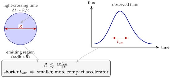
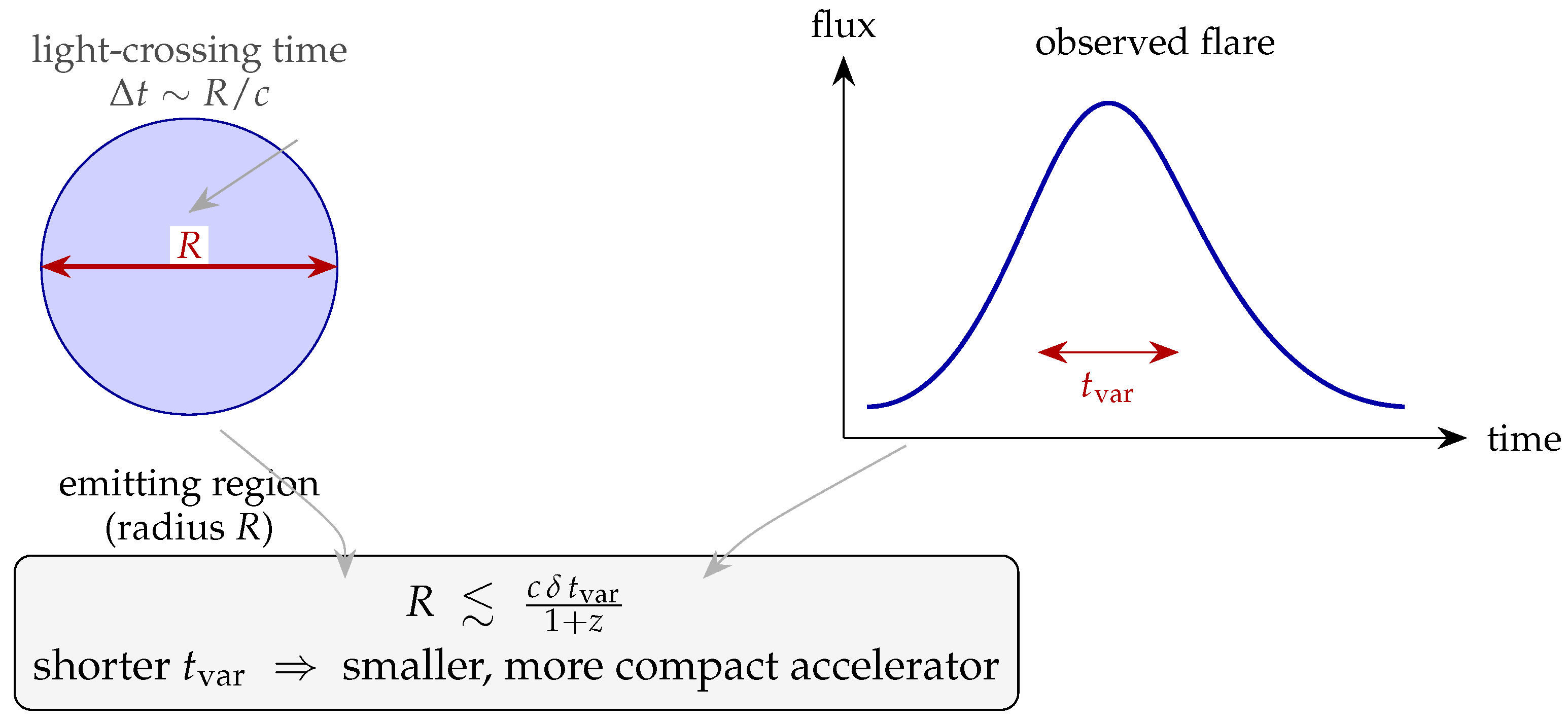
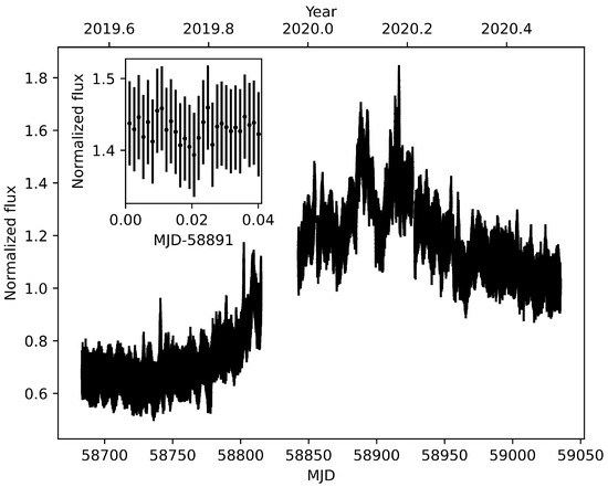
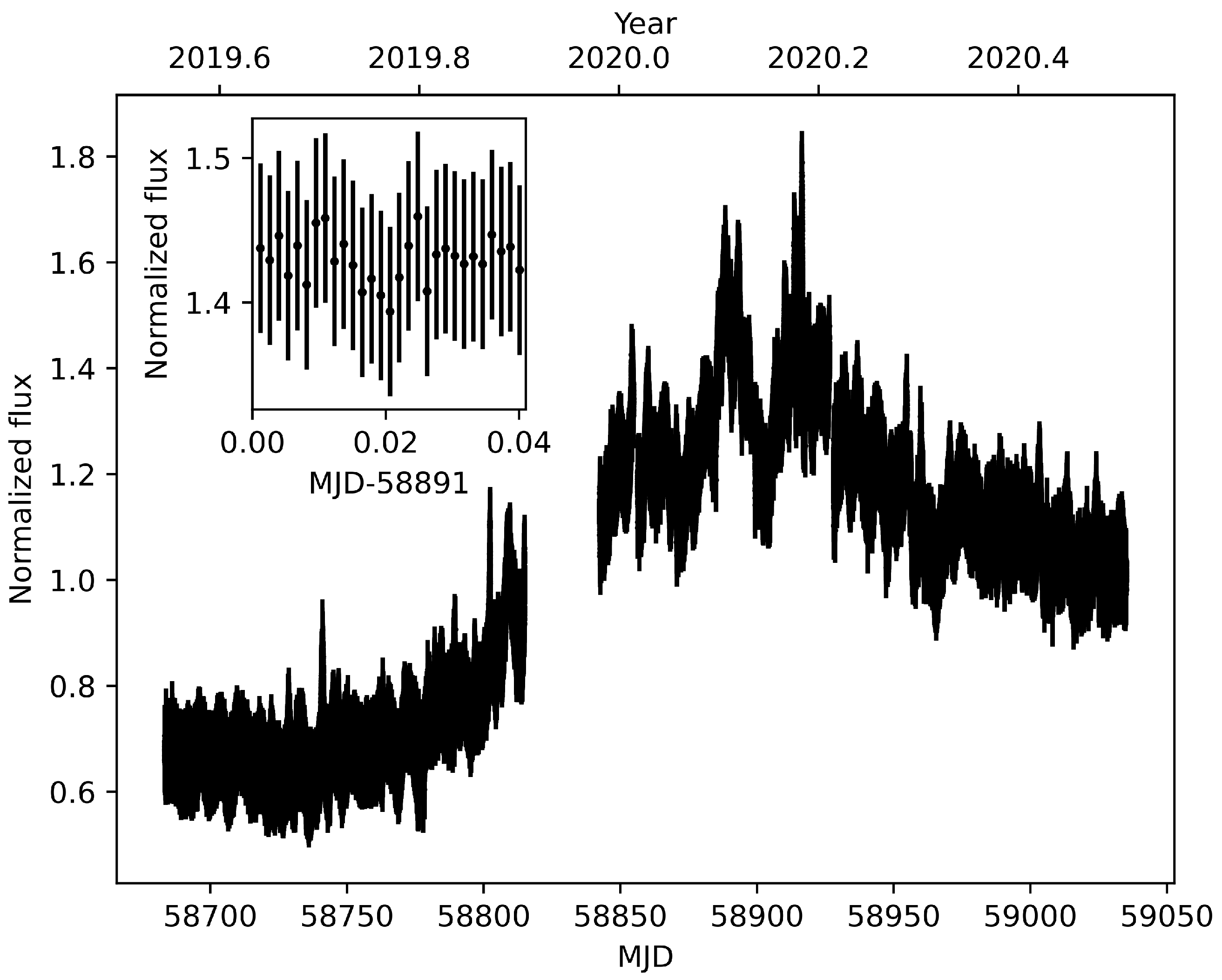
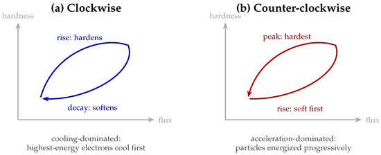
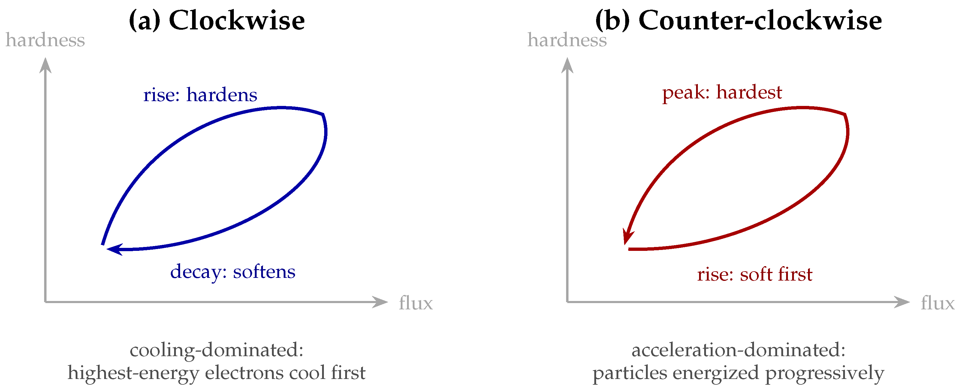
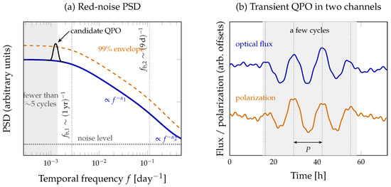
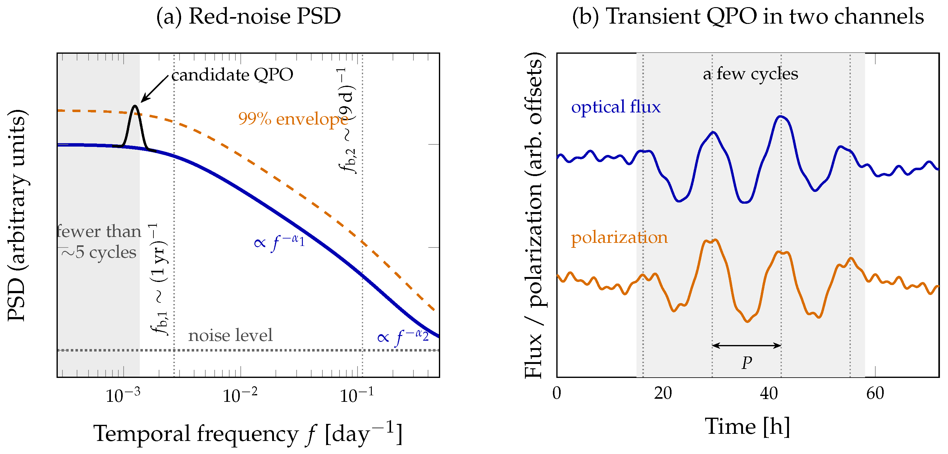
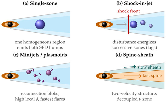
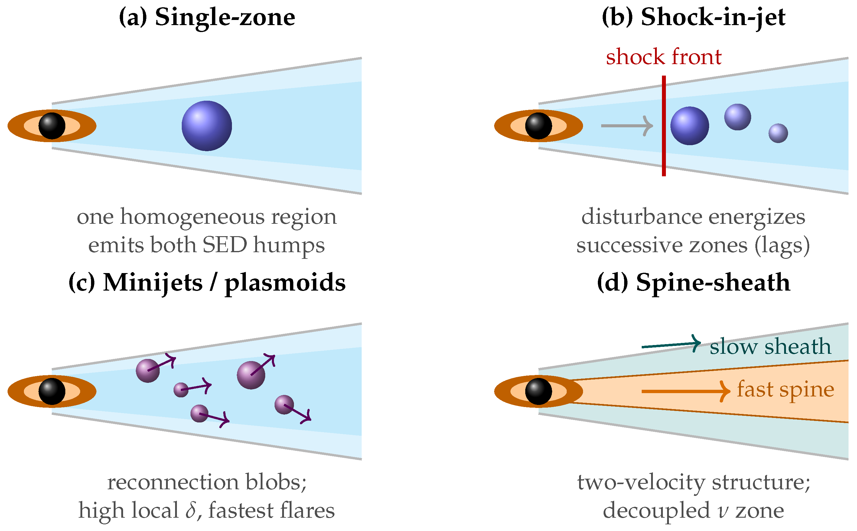
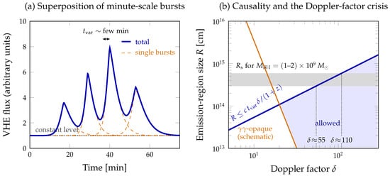
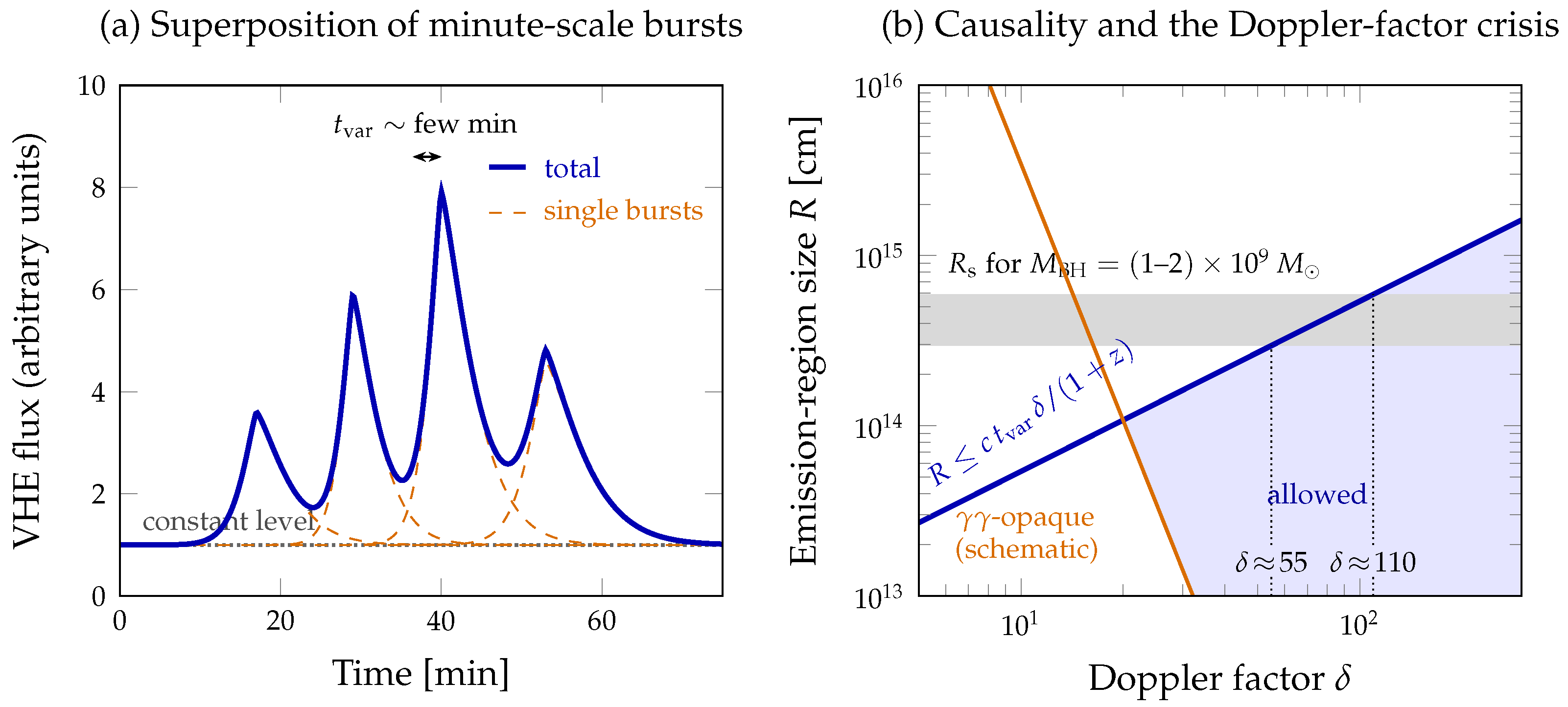
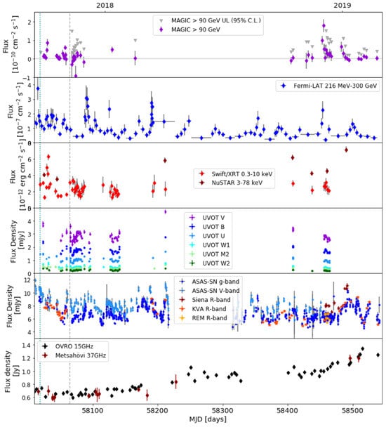
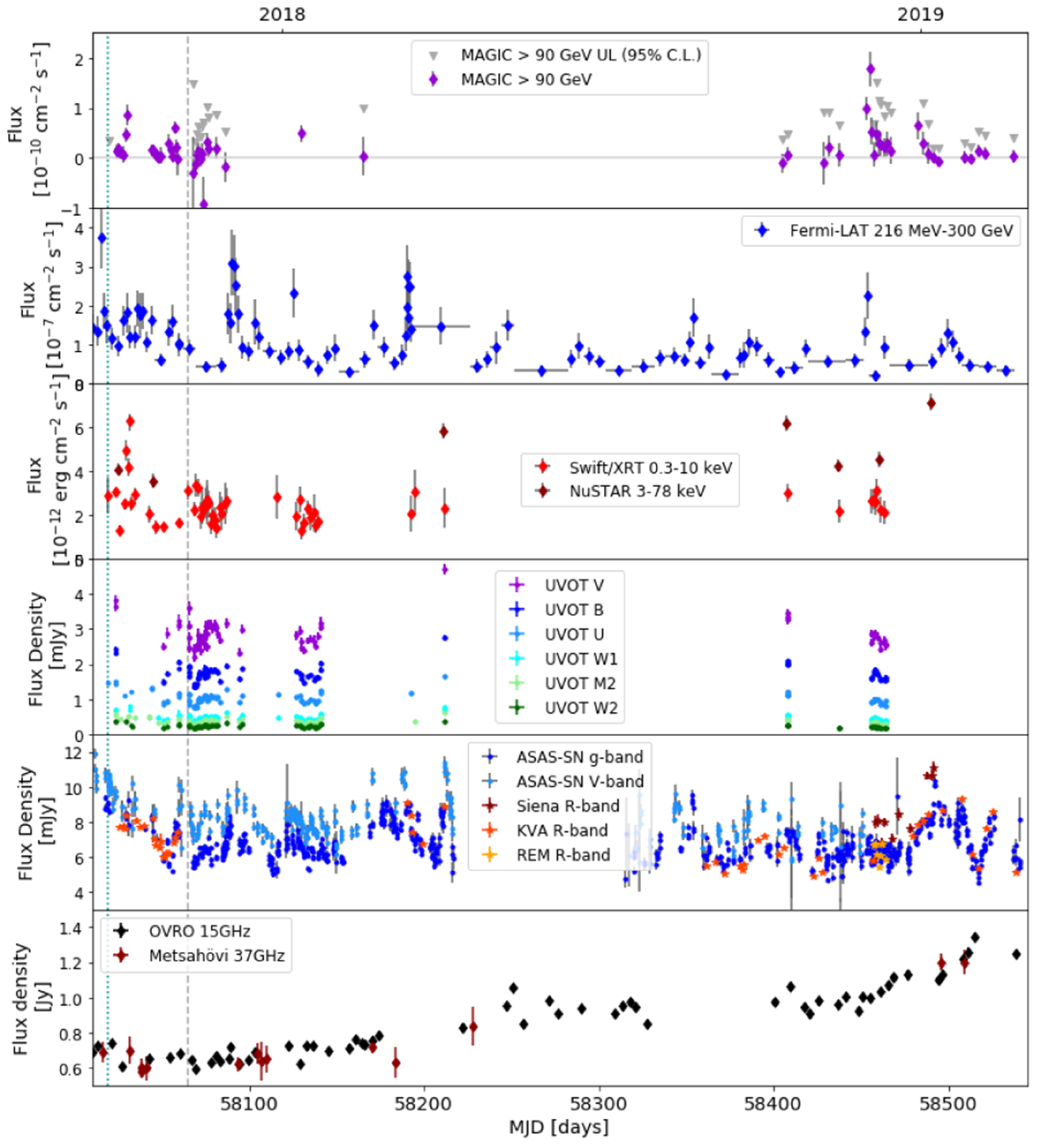
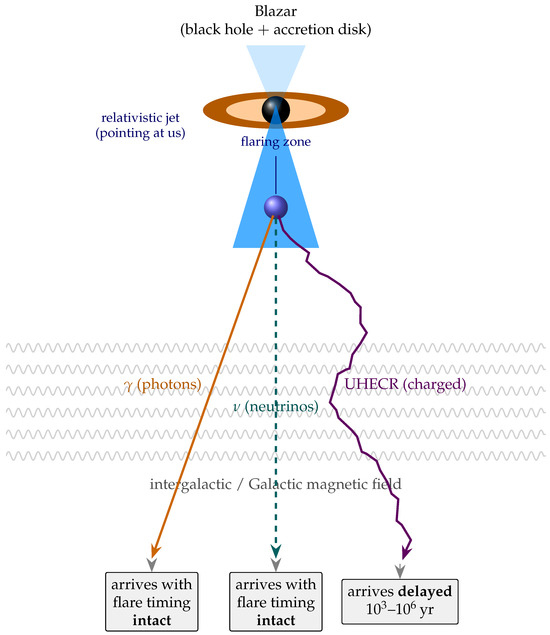
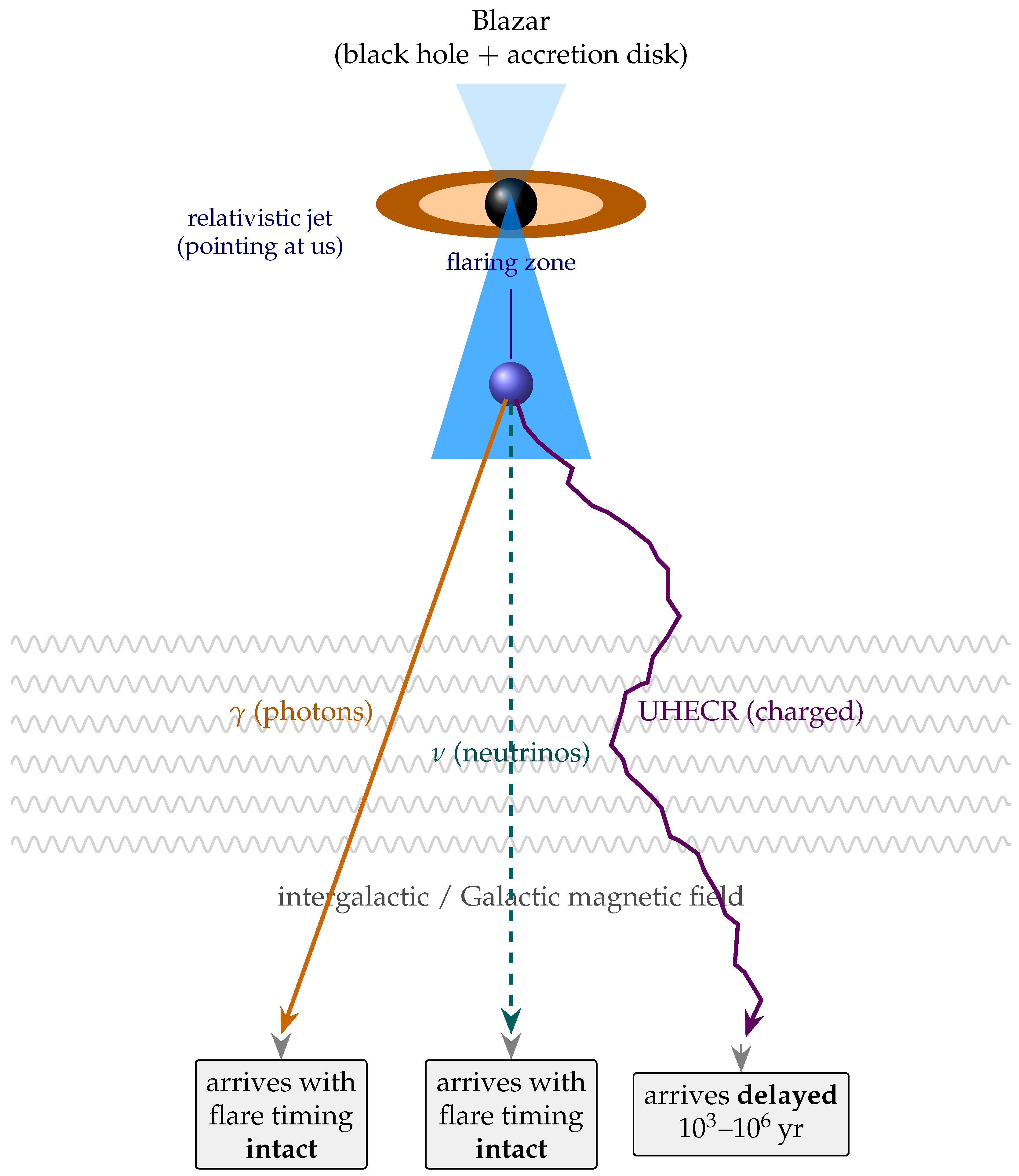

Disclaimer/Publisher’s Note: The statements, opinions and data contained in all publications are solely those of the individual author(s) and contributor(s) and not of MDPI and/or the editor(s). MDPI and/or the editor(s) disclaim responsibility for any injury to people or property resulting from any ideas, methods, instructions or products referred to in the content. |
© 2026 by the author. Licensee MDPI, Basel, Switzerland. This article is an open access article distributed under the terms and conditions of the Creative Commons Attribution (CC BY) license.