Robustness of U-Net Retinal Layer Segmentation to Controlled OCT Image Degradation

Abstract

Background: Optical coherence tomography (OCT) retinal layer segmentation supports quantitative clinical assessment, but its robustness to different image degradation has not been systematically characterized. Methods: This study evaluates a U-Net trained on unmodified OCT5k scans under seven synthetic degradation families at five family-specific severity levels. The test set included 315 held-out B-scans from nine cases, with three cases each of age-related macular degeneration, diabetic macular edema, and healthy retinas. After ordered boundary decoding, two primary outcomes were calculated: boundary mean absolute error (MAE, pixels) and internal-layer Dice. Results: Clean images yielded macro-MAE of 3.66 pixels and macro-Dice of 0.934. At severity 5, MAE increased in five families and Dice decreased in all seven. Gaussian noise, contrast reduction, and global attenuation produced the largest deterioration, with macro-MAE/macro-Dice values of 94.35/0.715, 236.81/0.044, and 112.32/0.0004, respectively. Adjusted paired tests showed statistically significant deterioration in both outcomes for these three families; macro-Dice also showed declines under defocus, shadowing, and axial-resolution reduction, while speckle showed no significant change. Conclusions: These results indicate corruption- and metric-specific vulnerability in the tested U-Net. This study may inform the development of automated OCT image-quality screening. Before clinical use, these findings may be evaluated on other segmentation models, larger datasets, additional OCT devices, and with naturally occurring acquisition artifacts.

1. Introduction

Optical coherence tomography (OCT) [1], a non-invasive and high-resolution imaging technology, is integral to the diagnosis and longitudinal assessment of retinal disease. Retinal morphology and layer thickness are common biomarkers used for diagnosis, particularly in diseases such as age-related macular degeneration (AMD) [2], diabetic macular edema (DME) [3,4], and glaucoma [5]. Robust OCT analysis relies on localization of anatomical boundaries.

Manual delineation is labor-intensive and subject to variability between clinicians. Therefore, automated segmentation has become central to quantitative OCT analysis. Before the deep learning renaissance, automatic retinal layer segmentation was largely driven by classical image processing techniques [6,7,8,9,10]. More recently, deep learning methods have demonstrated high accuracy on benchmark datasets [11], including convolutional networks [12], transformer-based approaches [13], and U-Net [14,15].

OCT is susceptible to image-quality deterioration due to various acquisition and optical factors, including low signal strength, speckle noise, defocus, depolarization, illumination or beam placement problems, media opacity, shadowing, motion, and reduced contrast [16,17,18]. Such factors have long been identified as important threats to quantitative interpretation of OCT images [19,20].

Prior work has established a relationship between image quality and automatic image analysis. Heikka demonstrated algorithm- and layer-dependent susceptibility to reduced image quality [21]. A subsequent study similarly showed that image quality affects the utility of OCT-derived retinal thickness measurements, particularly retinal nerve fiber layer thickness [22]. Optical degradation has also been studied in the context of deep learning segmentation [23]. Statistical work has also demonstrated a fundamental relationship between OCT signal/noise characteristics and an achievable retinal-boundary localization accuracy [24].

While prior studies have established that image quality matters for layer segmentation accuracy, there remains a gap in systematic characterization of the degradation response across multiple relevant corruption types with quantified degradation curves [11]. Indeed, in a study comparing U-Net-based architectures for automatic retinal layer segmentation across multiple datasets, the authors note worse performance (i.e., “greater variability”) in one AMD dataset that they hypothesize can be explained by lower average image quality, specifically more noise [15]. This paper seeks to examine that hypothesis by systematically characterizing the effect of image quality on segmentation accuracy.

A recently published dataset, OCT5k [25], enables a systematic analysis of image quality and the reliability of automated retinal layer segmentation. OCT5k contains 1672 B-scans from 60 volumes and includes healthy, AMD, and DME patients. Each B-scan is manually annotated by three graders, including five retinal boundaries. Importantly, this multi-grader approach allows algorithmic errors to be interpreted relative to observer disagreement rather than only an absolute pixel error. The effect of image degradation on layer segmentation using the OCT5k dataset has not previously been reported.

The aim of this study is to quantify the effect of controlled OCT image degradation on automated retinal-layer segmentation. This paper will identify degradation- and boundary-specific vulnerabilities and compare model localization error against human inter-grader variability.

2. Materials and Methods

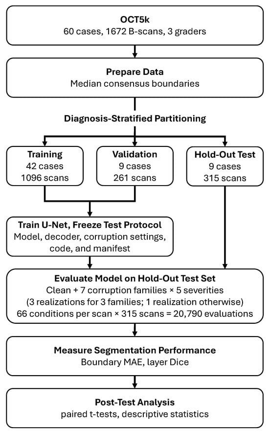
This study evaluates the performance of a U-Net segmentation model on computationally degraded OCT retinal images and annotations from OCT5k [25]. The data includes images from healthy, AMD, and DME patients. A U-Net segmentor was trained on the training and validation partitions without simulated image corruption. The trained model was evaluated across seven image corruption types, each with five severity levels. Two primary outcomes are examined: mean absolute errors (MAEs) for each of the pixel boundaries and Dice coefficients for the four internal regions. Figure 1 outlines the general workflow, and the following sections describe the experiment in detail.

Figure 1. OCT5k data, including three clinicians’ manual segmentation, is used to generate consensus retinal boundaries as ground truth, then partitioned and used to train a U-Net segmentation model. Seven corruption families (three of them having three realizations) each with five severity levels are used to degrade the images. MAE and layer Dice are used assess U-Net segmentation performance.

2.1. Dataset and Partitioning

The experiment includes 60 diagnostic cases with 1672 B-scans total: 739 AMD, 403 DME, and 530 healthy. Each image is a single channel, $512\times 512$-pixels, with three sets of manual clinician-drawn retinal boundary coordinates and segmentation masks. Five annotated boundaries include: inner limiting membrane (ILM), outer plexiform layer (OPL), inner segment-outer segment (IS-OS), inner boundary of retinal pigment epithelium (IBRPE) and outer boundary of retinal pigment epithelium (OBRPE). The diagnosis of all 60 cases was indicated by the directory structure and included 21 AMD, 19 DME, and 20 healthy patients (a slight discrepancy from the 20 volumes per diagnostic group reported in the original paper).

According to the original OCT5k paper [25], the sixty cases included in the OCT5k dataset were all visually assessed by clinicians and characterized as either “good” or “medium” quality; no “bad” quality images were included. The primary robustness analysis in this study compares each degraded scan with its own unmodified baseline. This paired comparison accounts for each scan’s starting performance, although it does not rule out the possibility that scans with different starting characteristics may respond differently to a given degradation.

The cases were pseudo-randomly assigned to training (~70%), validation (~15%), and test (~15%) partitions within each diagnostic class. All B-scans from one case were kept within the same partition. The result was 42 training cases (1096 B-scans), 9 validation cases (261 B-scans), and 9 test cases (315 B-scans). The test set included three cases for each diagnosis, but robustness outcomes were analyzed across the nine cases together; no diagnosis-specific robustness analyses were performed. The split was saved and reused throughout the experiment. See Table 1.

Table 1. Data partitioning by diagnostic label. Entries are numbers of cases/B-scans.

Diagnosis	Training	Validation	Test	Total
AMD	15/499	3/57	3/183	21/739
DME	13/247	3/99	3/57	19/403
Healthy	14/350	3/105	3/75	20/530
Total	42/1096	9/261	9/315	60/1672

2.2. Consensus Boundaries and Region Labels

As a prerequisite to training a U-Net model for layer segmentation, ground-truth boundaries were first derived from the three clinical annotations. For scan i, let $b_{igk}\left(x\right)$ denote the axial coordinate of boundary k at lateral position ( A-scan, or more precisely image columns) x for grader $g\in \{1,2,3\}$. Let $V_i$ be the set of image columns for which all five boundaries were valid, maintaining the expected top-to-bottom anatomical arrangement for each of the graders. The reference boundary was then calculated as the coordinate-wise median,

$$b_{ik}^{\mathrm{ref}}\left(x\right)={\mathrm{median}}_{g\in \{1,2,3\}}{b}_{igk}\left(x\right),x\in V_i,k=1,\dots ,5.$$

(1)

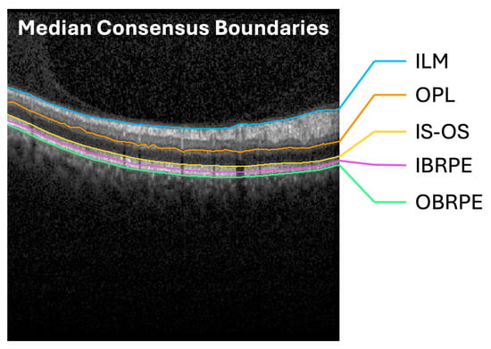
Thus, every evaluated column had contributions from all three graders. Columns with invalid boundaries were excluded from training and evaluation. Invalid columns were excluded from training labels and reference-based evaluation (0.40% of all columns). See Figure 2 for representative consensus boundaries.

Figure 2. The median of three clinicians’ boundary annotations was taken as the consensus boundary for the five boundaries in the B-scan images: (1) ILM, (2) OPL, (3) IS-OS, (4) IBRPE, and (5) OBRPE.

The five consensus boundaries defined six ordered region classes: above the ILM, ILM−OPL, OPL−IS-OS, IS-OS−IBRPE, IBRPE−OBRPE, and below the OBRPE. The four internal regions were used for the reported layer Dice scores; the two exterior regions were included in network training but excluded from the internal-layer Dice summary.

2.3. U-Net Architecture and Training

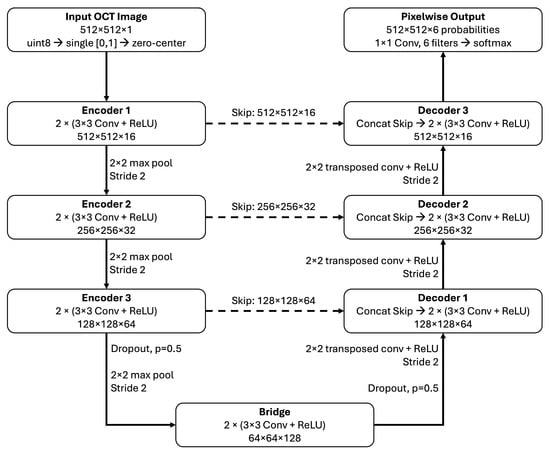
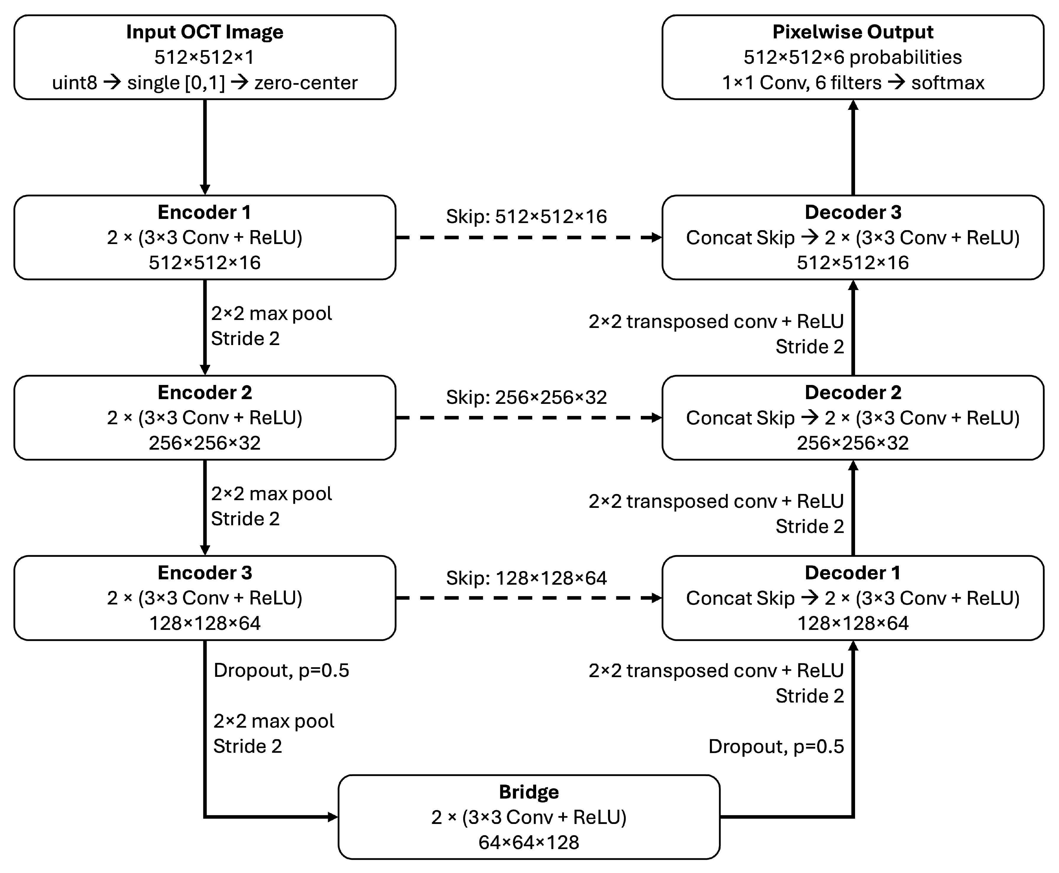
Images were used at their native $512\times 512$ resolution and scaled to single precision $[0,1]$ from 8-bit unsigned integer format, without minimum–maximum normalization. The segmentation baseline used the U-Net architecture [26] as implemented in MATLAB R2024b’s unetLayers function. The input is $512\times 512$-pixels and uses zero-centering normalization. The network is three encoders deep: (1) 16 filters, (2) 32 filters and (3) 64 filters, with 128 filters in the bridge. Encoder stages used pairs of $3\times 3$ convolutions with rectified linear unit activations and $2\times 2$ max pooling. The decoder used transposed convolutions for upsampling and skip connections to the corresponding encoder stages. Convolutions used same padding, and the final encoder stage and bridge included dropout with probability 0.5. A final $1\times 1$ convolution and softmax produced pixelwise class predictions with six possible classes. Convolution weights used He initialization, with initial biases set to zero. See Figure 3.

Figure 3. U-Net architecture for OCT retinal segmentation. Images are scaled to [0, 1] and zero-centered. Three encoder stages generated 16, 32, and 64 feature channels, followed by a bridge with 128 channels. Convolutional blocks contained two (3 × 3) convolutions, each followed by a rectified linear unit (ReLU), with same padding. Downsampling used (2 × 2) max pooling with stride 2. Decoder stages used (2 × 2) transposed convolutions with stride 2 and ReLU, followed by concatenation with the corresponding encoder features through skip connections (dashed arrows). Dropout (p = 0.5) was applied before the final max-pooling operation and after the bridge during training; skip features were extracted before dropout. A final (1 × 1) convolution and softmax produced six class probabilities per pixel. Dimensions indicate height × width × channels.

Training was performed with uncorrupted images and used the default, unweighted pixel classification cross-entropy loss, with undefined reference pixels ignored. The Adam optimizer was run for 30 epochs with a learning rate of ${10}^{-3}$ and a mini-batch size of two. Images were shuffled at each epoch. No explicit image augmentation, corruption augmentation, or class weighting was used. Other optimizer settings retained the defaults of the specified MATLAB release. MATLAB’s random generator was initialized with seed 20260927. Validation was scheduled every 548 training iterations, corresponding to one training epoch, and the network with the lowest validation loss was retained. The run completed 16,440 optimizer iterations, and the saved model corresponded to iteration 15,344, at epoch 28. The test partition was not used for checkpoint selection. Training was performed on a CPU using MATLAB R2024b Update 5 on an Apple-silicon platform.

2.4. Ordered Boundary Decoding

Region predictions were converted to boundaries algorithmically ensuring that the region labels were monotonically increasing through each image column. In each image column, the algorithm selected a nondecreasing sequence of region labels that minimized the number of changes to the raw predicted labels. The minimization was restricted to nondecreasing sequences of labels from 1 to 6, with the first and last rows constrained to classes 1 and 6, respectively. Here, $m(y,x)$ is the original predicted label at row y and column x, and $H=512$ is the image height.

$$\widehat{\mathbf{z}}\left(x\right)=\underset{\mathbf{z}}{\arg \min }{\displaystyle \sum _{y=1}^H}\mathbf{1}\{z_y\ne m(y,x)\}.$$

(2)

For example, if a U-Net labels a column as [1, 2, 3, 3, 2, 3, 4, 5, 6], the minimum number of changed labels is selected as the correct labels: [1, 2, 3, 3, 3, 3, 4, 5, 6]. Any ties go to the lowest predecessor state. Zero-thickness regions were allowed. See Table 2 for a simplified example calculation. Boundary k was extracted as $1+{\sum }_{y=1}^H\mathbf{1}\{{\widehat{z}}_y\left(x\right)\le k\}$.

Table 2. Simplified example of ordered boundary decoding for one image column. Each row represents a successive pixel position from top to bottom, and values denote the six predicted region classes. The original U-Net prediction contains a decreasing prediction (row 5 prediction = 2), which is disallowed. Three admissible corrections are shown, each preserving nondecreasing class order and fixing the first and last labels to classes 1 and 6, respectively. Arrows identify labels changed from the U-Net prediction. Candidates 1 and 2 each require two changes, whereas candidate 3, the selected output, requires one, the minimum necessary in this example. Nine rows are shown for illustration; the actual decoder processes all 512 rows of each image column.

Row y	U-Net Prediction	Candidate 1	Candidate 2	Candidate 3 *
1	1	1	1	1
2	2	2	2	2
3	3	→ 2 $\phantom{\to }$	3	3
4	3	→ 2 $\phantom{\to }$	3	3
5	$\phantom{\downarrow }$ 2 ↓	2	→ 4 $\phantom{\to }$	→ 3 $\phantom{\to }$
6	3	3	→ 4 $\phantom{\to }$	3
7	4	4	4	4
8	5	5	5	5
9	6	6	6	6
Number of Changes (→):		2	2	1

* Selected.

2.5. Controlled Image Degradations

Seven image corruption families were systematically examined across five severity levels: (1) speckle noise, (2) Gaussian noise, (3) Gaussian defocus blur, (4) contrast reduction, (5) global attenuation, (6) localized shadowing, and (7) reduced axial sampling resolution. The inclusion of all seven corruption types is supported by previous work and cited in Table 3 and Table 4. Each corruption family has a corresponding parameter to control its severity, also listed in Table 3. The range of parameters and their mapping to severity were not calibrated against OCT-acquired images. Instead, they were heuristically selected so that the segmentation model would be driven to failure, as a crash test of U-Net retinal layer segmentation for OCT images. Each corrupted condition was generated directly from the original image, without combining corruption families, and all outputs were clipped to $[0, 1]$ without subsequent contrast renormalization. Three corruption families (speckle-like noise, Gaussian noise, and shadowing) had at least one stochastic element and thus included three independently seeded realizations at each severity level. For each scan and severity, three realizations were generated using pseudorandom seeds derived deterministically from the scan identifier, degradation family, severity, and realization number, with base seed 20260927 (see reproducibility package); their scan-level metrics were averaged before aggregation across scans within cases. Including the unmodified image, this yielded $1+3\times 5\times 3+4\times 5=66$ evaluations per test B-scan, or 20,790 evaluations in total.

Table 3. Corruption parameters at severity levels 1–5.

Corruption	Varied Parameter	Severity Levels
		1	2	3	4	5
Speckle-like noise [24]	Noise standard deviation, ${\sigma }_1$	0.04	0.08	0.12	0.18	0.25
Gaussian noise [27]	Noise standard deviation, ${\sigma }_2$	0.01	0.02	0.04	0.06	0.09
Defocus blur [20]	Gaussian standard deviation (pixels), ${\sigma }_3$	0.5	1	1.5	2	3
Contrast reduction [28]	Fraction of contrast retained, $a_1$	0.85	0.70	0.55	0.40	0.25
Global attenuation [21]	Fraction of intensity retained, $a_2$	0.85	0.70	0.55	0.40	0.25
Shadowing [29]	Maximum fractional intensity loss, d	0.15	0.30	0.45	0.60	0.75
Axial resolution [30]	Retained height fraction, $a_3$	0.85	0.65	0.50	0.35	0.20

Table 4. Illustrative relationships between the synthetic corruption operations and possible clinical OCT appearances. The examples describe plausible analogies, not one-to-one mappings: the synthetic transformations do not reproduce specific device artifacts or establish their clinical frequency.

Synthetic Corruption	Possible Clinical Appearance	Possible Source or Mechanism in OCT	Relation to the Study Operation, Limitations, and Interpretation
Speckle-like noise	Granular intensity fluctuations within retinal tissue, particularly common around layer boundaries.	Speckle is inherent to coherent OCT imaging: light scattered from multiple tissue locations interferes at the detector. The speckle pattern can vary with the distribution of scatterers, scan geometry, and acquisition or averaging [31,32].	This study adds multiplicative random variation to the image. It represents increased speckle-like texture, not a specific disease or an established clinical state of “excess speckle.” Changes in the tissue scattering pattern can alter speckle, but do not necessarily increase its magnitude.
Gaussian noise	Random pixel-level fluctuations or a visibly noisier, lower signal-to-noise image.	OCT system noise can arise from detector and electronic noise, thermal noise, quantization, shot noise, and light-source intensity fluctuations [32].	The study adds independent Gaussian noise to the displayed image. This is a general noise stress test; real OCT noise sources have different statistical properties and are not necessarily independent, additive, or Gaussian in the displayed image. It should not be attributed to one particular device failure or patient condition.
Defocus blur	Less sharply defined retinal layers and reduced visibility of fine structure.	The retinal plane may be out of focus because of acquisition focus or alignment, refractive or optical factors, or other imaging conditions. Defocus is commonly recognized as a source of reduced OCT image quality [18,33].	The study applies Gaussian spatial blur. This approximates loss of fine detail but does not model the full optical point-spread function, a particular refractive error, or a specific scanner’s focusing behavior.
Contrast reduction	Reduced visual distinction between retinal layers or between adjacent structures.	Media opacity, including cataract or vitreous opacity, and ocular-surface or acquisition problems can reduce signal quality and make retinal structures harder to distinguish [18,33].	The study compresses image contrast around its mean. Real media opacity can cause scattering, attenuation, and other spatially varying effects; the contrast operation does not reproduce those mechanisms or their depth dependence.
Global attenuation	A generally dimmer B-scan with reduced signal across much of the image.	Diffuse signal loss can be associated with media opacity, dry eye, poor beam positioning or alignment, vignetting from a small pupil, or equipment and acquisition factors [18,33].	The study uniformly scales image intensity. This is a simplified model of generalized signal reduction; clinical attenuation may vary by location and depth and may occur together with blur or other image changes.
Shadowing	A dark region below a structure that attenuates or blocks the OCT beam.	Shadowing may occur beneath retinal vessels or structures such as drusen, hemorrhage, edema, and vitreous floaters [33,34].	The study applies a spatially localized intensity reduction. This approximates a shadow-like appearance but does not model the different optical interactions, shapes, or tissue-specific causes of clinical shadows.
Axial resolution	Reduced fine detail in the depth direction of the B-scan.	OCT axial resolution depends on system properties, including the source wavelength and spectral bandwidth; image sampling and reconstruction also affect the displayed axial detail [32].	The study vertically downsamples the image, applies antialiasing, and resizes it to the original dimensions. This reduces sampled axial detail; it does not simulate a specific OCT device’s native axial resolution or physical pixel spacing.

For an image I, speckle (multiplicative) noise was implemented as $I+{\sigma }_{1}Iϵ$ and additive noise as $I+{\sigma }_2ϵ$, where $ϵ(x,y)\sim \mathcal{N}(0,1)$ and ${\sigma }_{1,2}$ represents the standard deviation of the noise. Defocus blur was implemented using a Gaussian filter (replication boundary padding) with varying standard deviation, ${\sigma }_3$, for blur severity. Contrast reduction used $0.5+a_1(I-0.5)$, where $a_1$ was the fraction of the contrast retained, and global attenuation used $a_{2}I$. Shadowing multiplied each image column by $1-d\exp [-{(x-c)}^2/\left(2w^2\right)]$, where c was a randomly selected image column (uniform distribution) with width $w=0.06W$ (total image width, $W=512$), and d was varied for severity. Axial resolution was simulated by synthetically scaling down the image height to $a_{3}H$ and then resizing back to the original height using bilinear interpolation and MATLAB’s default antialiasing setting.

Corruption parameters and the decoding procedure were both assessed using validation data. The trained model and all inference settings were fixed before held-out test evaluation.

2.6. Outcome Measures

The primary outcomes were mean absolute errors (MAEs), in pixels, calculated for each image (i) and for each of the five retinal boundaries (k) (The OCT5k images did not include verified physical axial calibration; therefore, boundary errors are reported in pixels and were not converted to micrometers). For predicted boundary ${\widehat{b}}_{ik}$, the model-to-consensus error was calculated as

$${\mathrm{MAE}}_{ik}={\displaystyle \frac{1}{V_i}}\sum _{x\in V_i}\left|{\widehat{b}}_{ik}\left(x\right)-b_{ik}^{\mathrm{ref}}\left(x\right)\right|,$$

(3)

where $V_i$ is the number of valid image columns in a B-scan.

Inter-grader disagreement is calculated as grader-to-grader MAE ($MA{E}_{ik}^{g2g}$) for each image and boundary on the test set was calculated using exactly the same consensus-valid columns as the model evaluation. For each image (i) and boundary (k), the absolute differences for the three grader pairs were averaged:

$$MA{E}_{ik}^{g2g}={\displaystyle \frac{1}{3|V_i|}}\sum _{x\in V_i}\left(|b_{i1k}\left(x\right)-b_{i2k}\left(x\right)|+|b_{i1k}\left(x\right)-b_{i3k}\left(x\right)|+|b_{i2k}\left(x\right)-b_{i3k}\left(x\right)|\right).$$

(4)

Additionally, grader-to-consensus MAE ($MA{E}_{ik}^{\mathrm{g}2\mathrm{c}}$) was calculated for each image and boundary:

$$MA{E}_{ik}^{g2c}={\displaystyle \frac{1}{3|V_i|}}{\displaystyle \sum _{g=1}^3}\sum _{x\in V_i}\left|b_{ik}^{\left(g\right)}\left(x\right)-b_{ik}^{\mathrm{ref}}\left(x\right)\right|,$$

(5)

where $b_{ik}^{\left(g\right)}\left(x\right)$ is the position of boundary k in scan i marked by grader g, $b_{ik}^{\mathrm{ref}}\left(x\right)$ is the median position across the three graders, and $V_i$ is the set of valid columns.

Macro-MAEs are calculated for each image by averaging the five boundary-specific errors within a B-scan image and is used as an additional descriptive summary (physical axial spacing for the released images was not independently verified; errors were therefore not converted to micrometers).

A secondary segmentation outcome is the Dice coefficients for the four internal regions:

$${\mathrm{Dice}}_{i\mathsf{\ell }}={\displaystyle \frac{2|P_{i\mathsf{\ell }}\cap R_{i\mathsf{\ell }}|}{|P_{i\mathsf{\ell }}|+|R_{i\mathsf{\ell }}|}},$$

(6)

where $P_{i\mathsf{\ell }}$ and $R_{i\mathsf{\ell }}$ denote predicted and reference pixels in internal region ℓ. Dice was zero if exactly one region was empty and undefined if both were empty (this did not occur). An internal-region macro-Dice score for each B-scan was calculated by averaging the four region-specific scores. Exterior regions were excluded from this summary.

Case-weighted macro-Dice and macro-MAE are obtained by averaging the macro value across all the B-scans in a case, then averaging across all the cases. Because the ordered boundary decoder yields complete boundary predictions, all reference-valid columns were included in the evaluation, with incorrect boundary coordinates contributing to MAE and errors in the resulting region segmentation affecting Dice.

2.7. Statistical Analysis

For each stochastic degradation family–severity condition, the outcome measurements from the three seeded realizations were first averaged within each scan. Paired scan-level changes were then calculated relative to the same scan’s unmodified result. For all conditions, scan-level outcomes and changes were averaged within each case, and the nine case-level values were averaged with equal case weighting.

Uncertainty was summarized using 20,000 stratified whole-case bootstrap resamples. In each resample, three cases were drawn with replacement from each diagnostic group, retaining all scans for each selected case. The same resampled case indices were used for every outcome, condition, and paired clean-versus-degraded comparison. Pointwise 95% confidence intervals were calculated from the bootstrap distribution of the case-weighted means and are plotted against severity.

For each of the 35 degradation family–severity conditions, macro-MAE and macro-Dice were compared with their clean values. The paired comparisons used nine case-level observations (three cases per diagnostic group; 8 degrees of freedom) rather than treating the 315 B-scans as independent observations. The effect estimate was the mean of the nine paired case-level changes, with a two-sided 95% t-based confidence interval. Confidence intervals were pointwise and were not adjusted for multiple comparisons. Benjamini–Hochberg-adjusted [35] p-values were calculated across the 70 outcome–condition comparisons. BH-adjusted p-values below 0.05 were considered statistically significant, with a false discovery rate target of $q=0.05$. Worse performance is generally indicated by increased MAE and/or decreased Dice score. Layer-specific outcomes were also descriptively summarized.

The side-by-side summaries of model-to-consensus, grader-to-grader, and grader-to-consensus MAE are descriptive; no inferential tests compared these measures with one another. Because all three graders contributed to the median consensus, grader-to-consensus MAE is not an independent human-performance benchmark. These summaries do not define a human-performance threshold, clinical acceptability criterion, or equivalence between the model and graders.

Model training used MATLAB R2024b Update 5, and the completed held-out benchmark and statistical analysis used R2026a Update 4. The experiment pipeline used the Deep Learning Toolbox, Computer Vision Toolbox, and Image Processing Toolbox.

3. Results

3.1. Unmodified Image Segmentation Performance

A baseline of segmentation was first established using the trained U-Net model deployed on the test set. The test set included 315 B-scans from 9 cases: 3 AMD cases with 183 images, 3 DME cases with 57 images, and 3 healthy cases with 75 images. For unmodified images, the average case-weighted (i.e., averaged across each case, and each case weighted equally) macro-MAE value was 3.66 pixels, with an observed range of 0.63–23.41 pixels across the nine case averages. The average case-weighted macro-Dice coefficient across all test images was 0.934 for unmodified images (Table 5).

Table 5. Baseline image test-set boundary localization and retinal-band overlap. Values are equally case-weighted means ± standard deviations across the nine held-out cases. Boundary MAEs are expressed in pixels. Macro MAEs (bold) are the unweighted mean of the five MAEs within each case, then averaged across cases. Dice rows report overlap for the retinal band between the indicated boundaries. Macro-Dice (bold) is the unweighted mean of the four bands’ Dice values within each case, then averaged across cases. These are descriptive statistics only.

Boundary	Model-to-Consensus	Grader-to-Grader	Grader-to-Consensus	Dice Coefficient
	MAE	MAEg2g	MAEg2c	Dice
ILM	$3.94\pm 9.28$	$0.93\pm 0.10$	$0.47\pm 0.05$
				$0.964\pm 0.025$
OPL	$4.52\pm 8.45$	$1.68\pm 0.55$	$0.84\pm 0.27$
				$0.957\pm 0.024$
IS-OS	$3.18\pm 6.74$	$0.86\pm 0.12$	$0.43\pm 0.06$
				$0.921\pm 0.026$
IBRPE	$3.24\pm 6.42$	$0.91\pm 0.20$	$0.46\pm 0.10$
				$0.893\pm 0.026$
OBRPE	$3.41\pm 6.26$	$0.92\pm 0.09$	$0.46\pm 0.04$
Macro	$\mathbf{3.66}\pm \mathbf{7.42}$	$\mathbf{1.06}\pm \mathbf{0.15}$	$\mathbf{0.53}\pm \mathbf{0.07}$	$\mathbf{0.934}\pm \mathbf{0.024}$

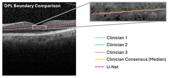
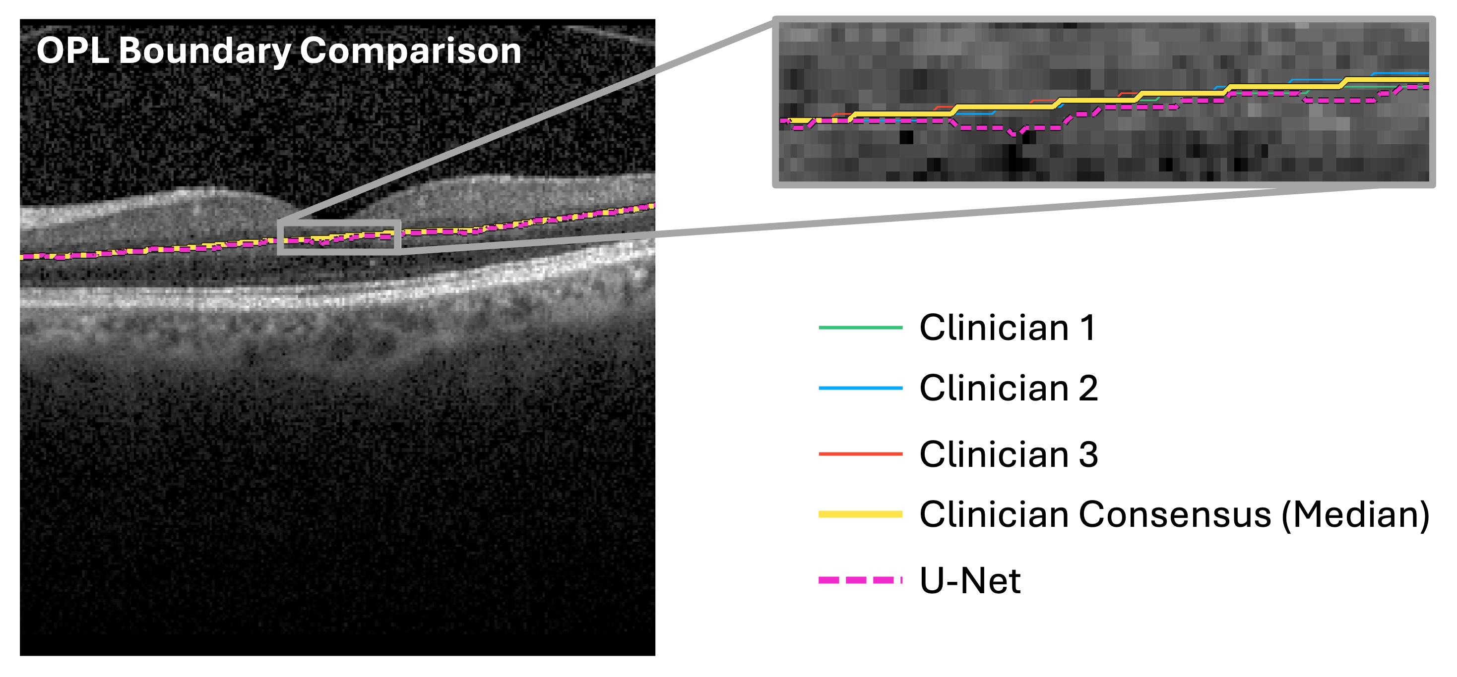
The average case-weighted model-to-consensus disagreement ($MAE$) was 3.66 pixels, case-weighted grader-to-grader disagreement ($MA{E}^{g2g}$) was 1.06 pixels, and case-weighted grader-to-consensus disagreement ($MA{E}^{g2c}$) was 0.53 pixels. The OPL had the largest mean model-to-consensus MAE (4.52 pixels), grader-to-grader MAE (1.68 pixels), and grader-to-consensus MAE (0.84). See Figure 4 and Table 5.

Figure 4. Example clinician, consensus, and U-Net-drawn OPL boundary, overlaid on a healthy retina (case: healthy 13, image: 10). The OPL boundary had the largest MAE of all MAE measurements.

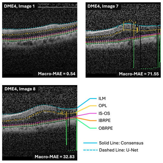
One test case, DME4 (Figure 5), had a clean macro-MAE of 23.411 pixels, compared with 0.631–2.093 pixels for the other eight cases. Including DME4, the equal-case mean clean macro-MAE was 3.658 pixels and the mean macro-Dice was 0.9340; after excluding DME4, these values were 1.189 pixels and 0.9412, respectively. DME4 also had the highest grader-to-grader and grader-to-consensus disagreement (1.33 and 0.67 pixels, respectively), consistent with greater difficulty in consistently delineating this case. These observations alone did not provide a sufficient basis for excluding DME4 as an outlier.

Figure 5. Case DME4 exhibited worse segmentation performance than all other cases included in the test set, as indicated by high MAE values. However, DME4 is included in all pairwise analyses in this study.

To assess the influence of DME4, paired analysis was performed again after excluding this case. For each remaining case, changes in macro-MAE and macro-Dice were calculated relative to that case’s unmodified images; the eight case-level changes were compared with zero using two-sided paired Student’s t-tests. BH adjustment was applied across the same comparisons as in the primary analysis. Supplementary Table S2 reports the mean paired changes and BH-adjusted p-values for all seven degradation families at all five severity levels.

In this sensitivity analysis of DME4, Gaussian noise degradation remained significant for both outcomes at severity 5, contrast reduction at severity 3 for macro-MAE and severity 2 for macro-Dice, and global attenuation at severity 4 for both outcomes. No comparison that was significant in the primary analysis became non-significant after excluding DME4. The leave-DME4-out analysis did, however, identify additional significant comparisons: macro-Dice for speckle-like noise at severities 3–5; macro-MAE for defocus blur at severity 5 and macro-Dice at severities 2 and 5; macro-MAE for shadowing at severity 5 and macro-Dice at severity 4; and macro-MAE for axial-resolution reduction at severity 5 and macro-Dice at severity 1.

At severity 5, the lower mean macro-MAE observed with DME4 included under defocus blur and axial-resolution reduction was driven by that case, whose paired changes were −12.14 and −14.43 pixels, respectively. In the other eight cases, mean macro-MAE increased by 1.112 pixels under defocus blur and 0.855 pixels under axial-resolution reduction, with all eight cases showing an increase in each condition. Macro-Dice was lower than the clean value in all nine cases at severity 5 for each degradation family, and the mean decrease remained after excluding DME4.

DME4 was retained in the primary analysis; the sensitivity analysis shows that its inclusion moderated some effects without changing the principal findings of this study.

3.2. Segmentation Response to Image Degradation

Across all degradation families and at severity level 5, mean macro-MAE increased for five of seven degradation families, and mean macro-Dice decreased for all seven (Table 6). Contrast reduction, attenuation, and Gaussian noise yielded the highest macro-MAEs, and in a BH-adjusted two-sided paired t-test between the unmodified baseline images and severity level 5, the difference in means was significantly different.

Table 6. Macro-MAE and macro-Dice means for severity level 5 image degradations compared to the unmodified baseline. Using a two-sided paired t-test with Benjamini–Hochberg adjustment, $\alpha =0.05$, three degradations produced significant differences in both measures: Gaussian noise, contrast reduction, and global attenuation.

Corruption (Severity 5)	Macro-MAE			Macro-Dice
	Mean	$\Delta$ Mean	# Increased	Mean	$\Delta$ Mean	# Decreased
Unmodified baseline	3.66	–	–	0.934	–	–
Speckle-like noise	7.45	+3.79	8/9	0.912	$-0.022$	9/9
Gaussian noise	94.35	+90.70 *	9/9	0.715	−0.219 *	9/9
Defocus blur	3.30	$-0.36$	8/9	0.878	−0.056	9/9
Contrast reduction	236.81	+233.15 *	9/9	0.044	−0.890 *	9/9
Global attenuation	112.32	+108.67 *	9/9	0.000	−0.934 *	9/9
Shadowing	4.84	+1.18	8/9	0.913	−0.021 *	9/9
Axial resolution	2.81	$-0.84$	8/9	0.885	−0.049 *	9/9

* BH-adjusted $p<0.05$.

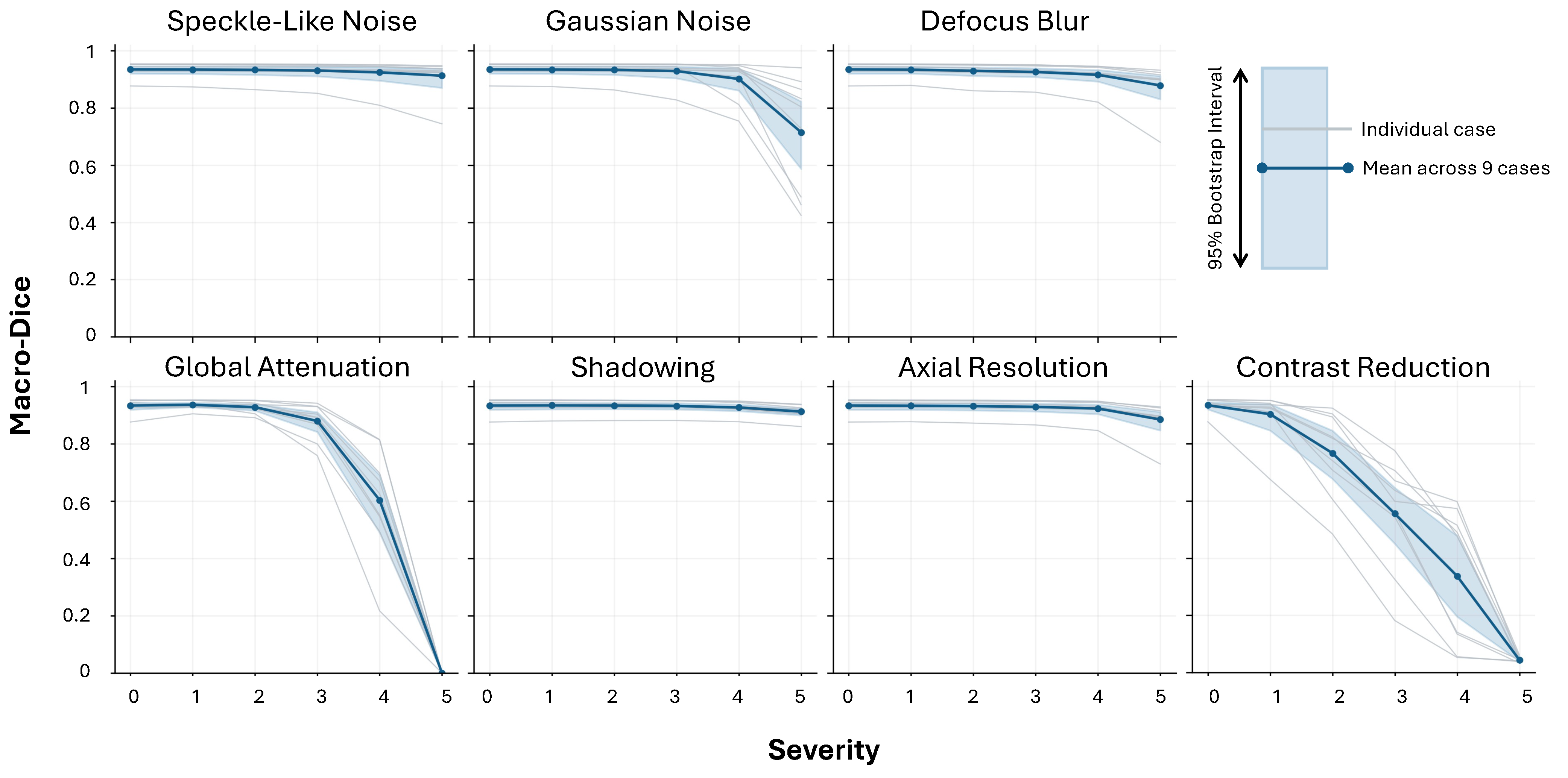
Across all severity levels and degradation families, the mean macro-Dice showed more consistent differences than the mean macro-MAE. The severity level at which statistically significant differences in the mean macro-Dice (compared to unmodified baseline images) first appeared varied: severity level 2 (axial resolution and contrast reduction), severity level 3 (defocus blur), severity level 4 (global attenuation), and severity level 5 (Gaussian noise and shadowing). Speckle-like noise did not exhibit any statistically significant differences at any severity level for macro-MAE or macro-Dice (Table 7). Table 8 lists the first significant MAE increase and Dice decrease for each degradation level and their corresponding degradation parameters. Supplementary Table S1 reports all 70 paired t-test confidence intervals, p-values, and BH-adjusted p-values.

Table 7. Severity levels at which a two-sided paired t-test between mean macro-MAE or mean macro-Dice in the degraded images versus the unmodified images yielded a significant difference ($\alpha =0.05$). Significant differences (BH-adjusted $p<0.05$) are indicated by a check mark, ✓.

Corruption	Macro-MAE					Macro-Dice
	1	2	3	4	5	1	2	3	4	5
Speckle-like noise
Gaussian noise					✓					✓
Defocus blur								✓	✓
Contrast reduction			✓	✓	✓		✓	✓	✓	✓
Global attenuation				✓	✓				✓	✓
Shadowing										✓
Axial resolution							✓	✓	✓	✓

✓ = BH-adjusted $p<0.05$.

Table 8. First tested corruption setting with significant worsening relative to the unmodified condition. Degradations without a significant difference across all severities are marked with –. All p-values are BH-adjusted.

Degradation	Macro-MAE Increase			Macro-Dice Decrease
	Severity	Parameter	p-Value	Severity	Parameter	p-Value
Speckle-like noise	–	–	–	–	–	–
Gaussian noise	5	${\sigma }_2=0.09$	0.0246	5	${\sigma }_2=0.09$	0.0297
Defocus blur	–	–	–	3	${\sigma }_3=1.5$	0.0131
Contrast reduction	3	$a_1=0.55$	0.0329	2	$a_1=0.70$	0.0237
Global attenuation	4	$a_2=0.40$	0.0212	4	$a_2=0.40$	0.0046
Shadowing	–	–	–	5	$d=0.75$	0.0008
Axial resolution	–	–	–	2	$a_3=0.65$	0.0019

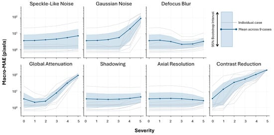
Contrast reduction demonstrated progressive deterioration across all severity levels, whereas other degradation families showed more reserved responses, particularly at low severity levels (Figure 6 and Figure 7).

Figure 6. Case-level macro-MAE across the five retinal boundaries for unmodified baseline scans (severity 0) and seven corruption families at severities 1–5. Gray lines indicate case-level means for the nine held-out test cases; the solid blue line is the mean across cases. The shaded region is the pointwise 95% interval from 20,000 stratified whole-case bootstrap resamples, sampling three cases with replacement within each diagnostic group. Severity scales are specific to each corruption family (Table 3) and are not directly comparable across families.

Figure 7. Case-level macro-Dice across the retinal layers for unmodified baseline scans (severity 0) and seven corruption families at severities 1–5. Gray lines indicate case-level means for the nine held-out test cases; the solid blue line is the mean across cases. The shaded region is the pointwise 95% interval from 20,000 stratified whole-case bootstrap resamples, sampling three cases with replacement within each diagnostic group. Severity scales are specific to each corruption family (Table 3) and are not directly comparable across families.

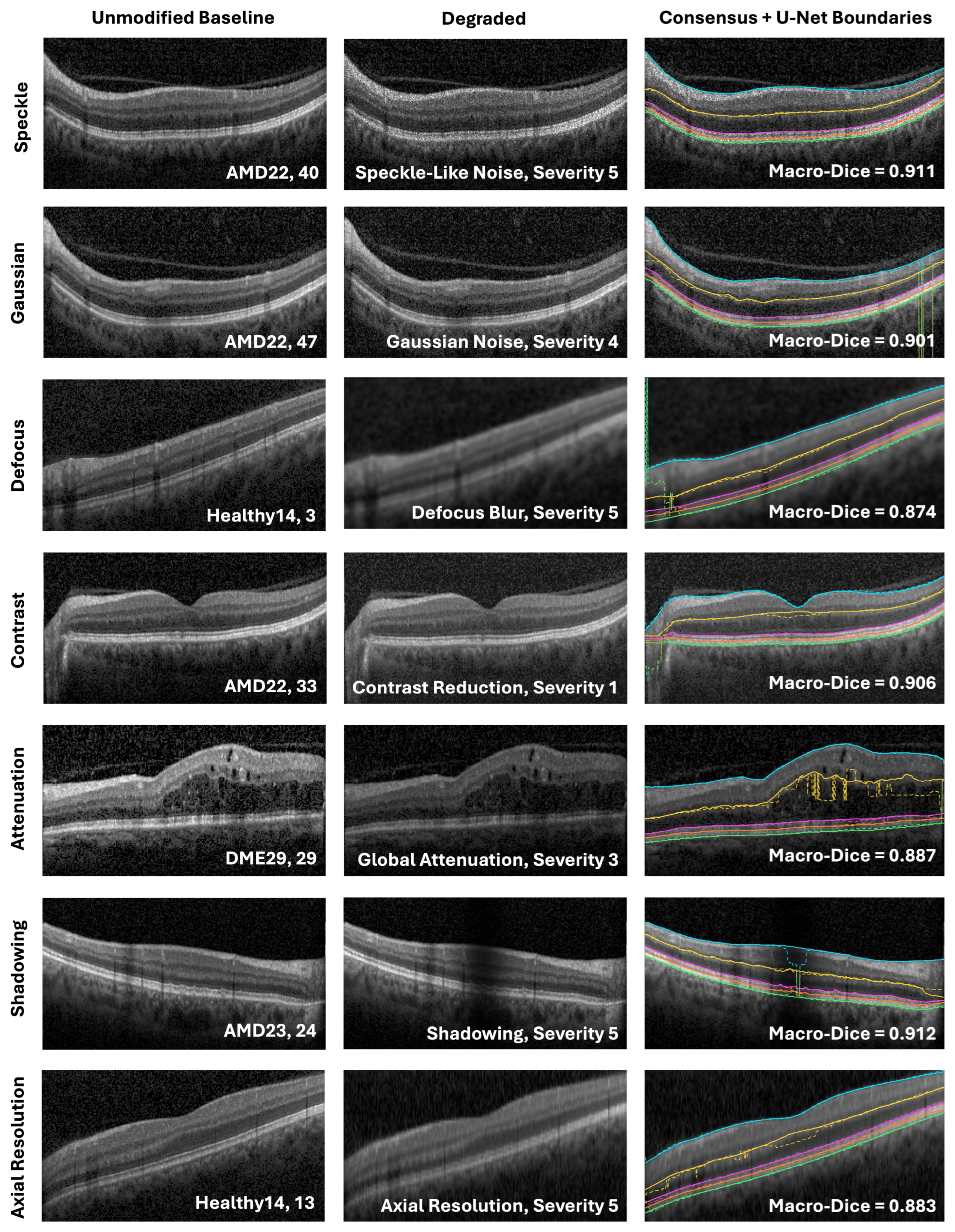
For visualization (Figure 8), the selected severity for each degradation family was the lowest tested level at which the equal-case mean macro-Dice fell by at least 0.02 from the unmodified baseline image mean (this was a display criterion only, not a statistical significance threshold). For each family, an example B-scan was chosen with a macro-Dice value close to the test-set mean at that severity. These examples illustrate image appearance and segmentation behavior near the average response after a point of >0.02 worse macro-Dice segmentation performance.

Figure 8. Representative B-scans before and after degradation at the selected severity, with consensus (solid) and U-Net (dashed) boundaries overlaid. Macro-Dice labels are for the displayed scans. Images are cropped for display only. Line colors and style are consistent with Figure 5.

3.3. Layer-Wise Analysis

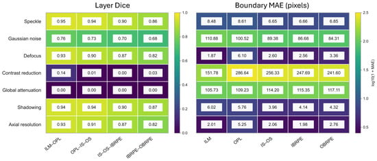
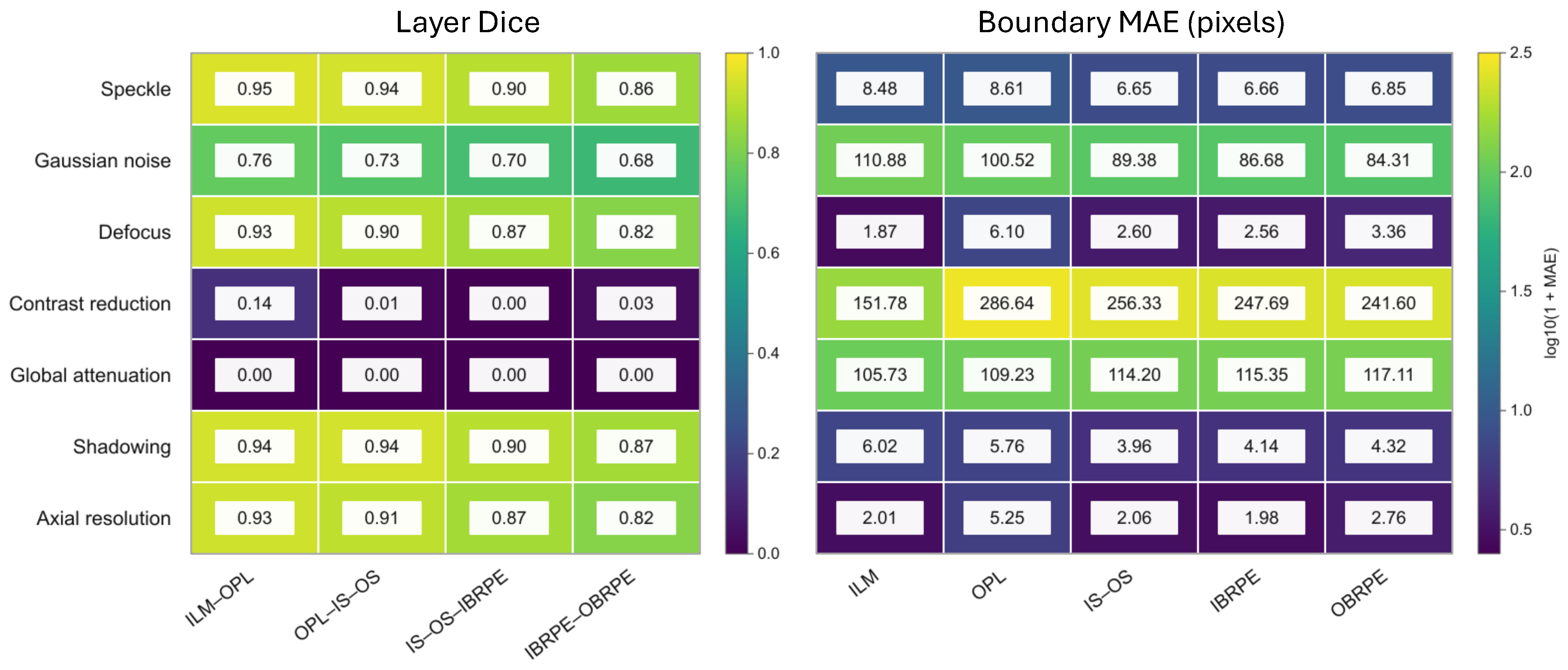
At severity 5, degradation effects varied across retinal boundaries (Figure 9). Gaussian noise produced its largest boundary MAE at the ILM (110.88 pixels), whereas contrast reduction produced its largest error at the OPL (286.64 pixels). With global attenuation, MAE increased from the ILM (105.73 pixels) toward the outer RPE boundary (117.11 pixels). Defocus blur also affected the OPL most strongly (6.10 pixels), while axial-resolution reduction produced its largest error at the OPL (5.25 pixels). Speckle-like noise and shadowing produced smaller boundary errors overall, although speckle-like noise reached 8.61 pixels at the OPL.

Figure 9. Boundary-specific MAE and internal-layer Dice at severity 5 for the seven corruption families. Values are case-weighted means across the nine held-out test cases; MAE is reported in pixels. Cell labels show raw MAE values, and color encodes ${\log }_{10}(1+\mathrm{MAE})$. Severity scales differ across corruption families, so severity 5 does not represent a common degradation strength.

Layer Dice generally decreased from the innermost to the outermost retinal band for speckle-like noise (0.95 to 0.86), Gaussian noise (0.76 to 0.68), defocus blur (0.93 to 0.82), shadowing (0.94 to 0.87), and axial-resolution reduction (0.93 to 0.82). Contrast reduction produced low Dice across all four bands (0.14, 0.01, 0.00, and 0.03); global attenuation reduced Dice to 0.00 for each band at the reported precision. These are case-weighted means at each corruption’s highest tested severity.

4. Discussion

This crash test study evaluated how controlled OCT image degradations affected U-Net segmentation. On unmodified images, the case-weighted macro-MAE was 3.66 pixels and the macro-Dice coefficient was 0.934. The severity at which performance first worsened varied by corruption family and outcome. Macro-Dice showed declines for six families: at intermediate settings for axial resolution ($a_3=0.65$), defocus blur (${\sigma }_3=1.5$ pixel), contrast reduction ($a_1=0.70$), and global attenuation ($a_2=0.40$), and only at the highest tested shadowing ($d=0.75$) and Gaussian noise levels (${\sigma }_2=0.09$). Macro-MAE showed increases for fewer families: contrast reduction ($a_1=0.55$), global attenuation ($a_2=0.40$), and Gaussian noise (${\sigma }_2=0.09$), with Gaussian noise appearing only at highest tested settings. Speckle-like noise showed no significant change in either metric. Dice sometimes showed degradation earlier than MAE.

The relationship between MAE and Dice depended on the corruption. At severity 5, defocus blur and axial-resolution degradation had mean MAE values below the clean mean, while their Dice coefficients were lower (0.878 and 0.885, respectively, compared with 0.934 for clean images). These two metrics respond differently to different degradation types, indicating that researchers developing automatic image quality algorithms should consider both output measures. MAE measures boundary-coordinate displacement, whereas Dice measures overlap of the regions between boundaries. Shifts can change band width or geometry differently, so lower mean MAE can coexist with lower Dice. A lower mean MAE alone should not be interpreted as better overall segmentation when Dice has declined. Conversely, the near-zero Dice values observed with severe contrast reduction and attenuation indicate that some degradations caused extensive failures in the predicted retinal regions.

The baseline image model-to-consensus macro-MAE was higher than both the pairwise grader disagreement (1.06 pixels) and grader-to-consensus disagreement (0.53 pixels). These quantities provide context for the model’s performance, but they are not independent measures of human accuracy: the same graders contributed to the consensus used as the reference. In particular, grader-to-consensus disagreement is expected to be lower in part because the consensus is constructed from the graders’ annotations. The comparison should therefore be interpreted as agreement with this study’s reference annotations rather than as a definitive threshold separating acceptable from unacceptable clinical performance.

The layer-wise summaries suggested that model error and grader disagreement varied across retinal boundaries. For example, the OPL had the largest clean model-to-consensus MAE and pairwise grader disagreement in the descriptive summaries. The high-severity results also showed boundary-specific variation across degradation families. Because these layer-wise differences were not tested inferentially, they should be treated as descriptive patterns that may guide future investigation rather than evidence that one boundary is systematically more vulnerable than another.

Retinal thickness, an important clinical indicator, is estimated from the separation between adjacent boundaries. Displacement of one boundary can bias the estimated thickness, while similar shifts of both boundaries may partly cancel in the thickness difference. Segmentation errors could therefore affect interpretation of retinal morphology or apparent longitudinal change. This study did not evaluate downstream thickness measurements or clinical decisions, but future work might expand the study to include diagnosis patterns.

Several limitations should be considered. First, the held-out test sample consisted of nine independent cases, with a total of 315 B-scans, and the t-test results should be interpreted cautiously given the small sample size. These findings are exploratory and may not generalize beyond the evaluated cases, U-Net model, and simulated degradations. The analysis evaluated one U-Net configuration and one OCT5k-derived test set; it does not establish how other architectures, training runs, devices, or patient populations would perform. The degradations were synthetic and applied using family-specific severity parameters. While the synthetic degradations were aimed at mimicking real-world artifacts, they cannot reproduce the full complexity or frequency of acquisition artifacts encountered in clinical practice. Moreover, clinical images may have multiple combined artifacts. (Such combinations may be explored in future studies.) Accordingly, this work does not claim to establish clinical degradation thresholds.

Only three test cases represented each diagnosis, and disease stage or severity was not analyzed. The results therefore do not establish performance across the full clinical variability of OCT images, including advanced AMD, severe DME, or other complex pathology. Larger independent cohorts spanning diagnostic subtypes and disease severity are needed to assess generalizability to these settings. Future work should evaluate the same corruption families on larger, independent datasets, including scans acquired on different devices and scans with naturally occurring quality problems. Evaluating multiple model architectures and repeated training runs would help determine whether the observed patterns are specific to this U-Net implementation or shared across segmentation methods. Such studies could establish whether image-quality indicators can reliably flag scans at risk of segmentation failure and whether those failures affect downstream retinal measurements.

Overall, controlled degradation revealed corruption-specific weaknesses in this U-Net pipeline, with particularly severe failures under strong noise, contrast reduction, and attenuation. These findings support evaluating image quality alongside automated segmentation performance, while further external validation is needed before translating the observed patterns into clinical quality-control rules.

5. Conclusions

Controlled image degradation revealed corruption-specific weaknesses in the evaluated U-Net pipeline on the held-out OCT5k cases. The largest failures occurred with severe contrast reduction and global attenuation, while Gaussian noise produced substantial increases in boundary error. Macro-Dice showed declines at lower tested settings than macro-MAE for several degradation families, and the measures did not always change in parallel, supporting the use of both overlap and boundary-distance outcomes. These findings describe one model tested on nine cases with synthetic degradations. The study did not evaluate a screening classifier, establish rejection thresholds, or demonstrate downstream clinical benefit; these applications require further validation using independent datasets and naturally occurring acquisition artifacts.

References

- Huang, D.; Swanson, E.A.; Lin, C.P.; Schuman, J.S.; Stinson, W.G.; Chang, W.; Hee, M.R.; Flotte, T.; Gregory, K.; Puliafito, C.A.; et al. Optical coherence tomography. Science 1991, 254, 1178–1181. [Google Scholar] [CrossRef] [Scilit] [PubMed]
- Heckenlaible, N.J.; Toomey, C.B.; Handa, J.T. OCT changes observed during the progression of early age-related macular degeneration. Ophthalmol. Sci. 2025, 5, 100615. [Google Scholar] [CrossRef] [Scilit] [PubMed]
- Parravano, M.; Cennamo, G.; Di Antonio, L.; Grassi, M.O.; Lupidi, M.; Rispoli, M.; Savastano, M.C.; Veritti, D.; Vujosevic, S. Multimodal imaging in diabetic retinopathy and macular edema: An update about biomarkers. Surv. Ophthalmol. 2024, 69, 893–904. [Google Scholar] [CrossRef] [Scilit] [PubMed]
- Suciu, C.I.; Suciu, V.I.; Nicoara, S.D. Optical coherence tomography (angiography) biomarkers in the assessment and monitoring of diabetic macular edema. J. Diabetes Res. 2020, 2020, 6655021. [Google Scholar] [CrossRef] [Scilit] [PubMed]
- Mayer, M.A.; Hornegger, J.; Mardin, C.Y.; Tornow, R.P. Retinal nerve fiber layer segmentation on FD-OCT scans of normal subjects and glaucoma patients. Biomed. Opt. Express 2010, 1, 1358–1383. [Google Scholar] [CrossRef] [Scilit] [PubMed]
- Koozekanani, D.; Boyer, K.; Roberts, C. Retinal thickness measurements from optical coherence tomography using a Markov boundary model. IEEE Trans. Med. Imaging 2001, 20, 900–916. [Google Scholar] [CrossRef] [PubMed]
- Ishikawa, H.; Stein, D.M.; Wollstein, G.; Beaton, S.; Fujimoto, J.G.; Schuman, J.S. Macular segmentation with optical coherence tomography. Investig. Ophthalmol. Vis. Sci. 2005, 46, 2012–2017. [Google Scholar] [CrossRef] [Scilit] [PubMed]
- Chan, A.; Duker, J.S.; Ishikawa, H.; Ko, T.H.; Schuman, J.S.; Fujimoto, J.G. Quantification of photoreceptor layer thickness in normal eyes using optical coherence tomography. Retina 2006, 26, 655. [Google Scholar] [CrossRef] [Scilit] [PubMed]
- Cabrera Fernández, D.; Salinas, H.M.; Puliafito, C.A. Automated detection of retinal layer structures on optical coherence tomography images. Opt. Express 2005, 13, 10200–10216. [Google Scholar] [CrossRef] [Scilit] [PubMed]
- Garvin, M.K.; Abràmoff, M.D.; Kardon, R.; Russell, S.R.; Wu, X.; Sonka, M. Intraretinal layer segmentation of macular optical coherence tomography images using optimal 3-D graph search. IEEE Trans. Med. Imaging 2008, 27, 1495–1505. [Google Scholar] [CrossRef] [Scilit] [PubMed]
- Zhang, H.; Yang, B.; Li, S.; Zhang, X.; Li, X.; Liu, T.; Higashita, R.; Liu, J. Retinal OCT image segmentation with deep learning: A review of advances, datasets, and evaluation metrics. Comput. Med. Imaging Graph. 2025, 123, 102539. [Google Scholar] [CrossRef] [Scilit] [PubMed]
- Roy, A.G.; Conjeti, S.; Karri, S.P.K.; Sheet, D.; Katouzian, A.; Wachinger, C.; Navab, N. ReLayNet: Retinal layer and fluid segmentation of macular optical coherence tomography using fully convolutional networks. Biomed. Opt. Express 2017, 8, 3627–3642. [Google Scholar] [CrossRef] [Scilit] [PubMed]
- Cao, G.; Zhang, S.; Mao, H.; Wu, Y.; Wang, D.; Dai, C. A single-step regression method based on transformer for retinal layer segmentation. Phys. Med. Biol. 2022, 67, 145008. [Google Scholar] [CrossRef] [Scilit] [PubMed]
- Wang, B.; Wei, W.; Qiu, S.; Wang, S.; Li, D.; He, H. Boundary aware U-Net for retinal layers segmentation in optical coherence tomography images. IEEE J. Biomed. Health Inform. 2021, 25, 3029–3040. [Google Scholar] [CrossRef] [Scilit] [PubMed]
- Kugelman, J.; Allman, J.; Read, S.A.; Vincent, S.J.; Tong, J.; Kalloniatis, M.; Chen, F.K.; Collins, M.J.; Alonso-Caneiro, D. A comparison of deep learning U-Net architectures for posterior segment OCT retinal layer segmentation. Sci. Rep. 2022, 12, 14888. [Google Scholar] [CrossRef] [Scilit] [PubMed]
- Chhablani, M.J.; Krishnan, M.T.; Sethi, M.V.; Kozak, I. Artifacts in optical coherence tomography. Saudi J. Ophthalmol. 2014, 28, 81–87. [Google Scholar] [CrossRef] [Scilit] [PubMed]
- Bazvand, F.; Ghassemi, F. Artifacts in macular optical coherence tomography. J. Curr. Ophthalmol. 2020, 32, 123. [Google Scholar] [CrossRef] [Scilit] [PubMed]
- Bayer, A.; Akman, A. Artifacts and anatomic variations in optical coherence tomography. Turk. J. Ophthalmol. 2020, 50, 99. [Google Scholar] [CrossRef] [Scilit] [PubMed]
- Tewarie, P.; Balk, L.; Costello, F.; Green, A.; Martin, R.; Schippling, S.; Petzold, A. The OSCAR-IB consensus criteria for retinal OCT quality assessment. PLoS ONE 2012, 7, e34823. [Google Scholar] [CrossRef] [Scilit] [PubMed]
- Somfai, G.M.; Salinas, H.M.; Puliafito, C.A.; Fernandez, D.C. Evaluation of potential image acquisition pitfalls during optical coherence tomography and their influence on retinal image segmentation. J. Biomed. Opt. 2007, 12, 041209. [Google Scholar] [CrossRef] [Scilit] [PubMed]
- Heikka, T.; Cense, B.; Jansonius, N.M. Retinal layer thicknesses retrieved with different segmentation algorithms from optical coherence tomography scans acquired under different signal-to-noise ratio conditions. Biomed. Opt. Express 2020, 11, 7079–7095. [Google Scholar] [CrossRef] [Scilit] [PubMed]
- Heikka, T.; Jansonius, N.M. Influence of signal-to-noise ratio, glaucoma stage and segmentation algorithm on OCT usability for quantifying layer thicknesses in the peripapillary retina. Acta Ophthalmol. 2023, 101, 251–260. [Google Scholar] [CrossRef] [Scilit] [PubMed]
- Allegrini, D.; Raimondi, R.; Sorrentino, T.; Tripepi, D.; Stradiotto, E.; Caruso, M.; De Rosa, F.P.; Romano, M.R. The effect of optical degradation from cataract using a new Deep Learning optical coherence tomography segmentation algorithm. Graefe’s Arch. Clin. Exp. Ophthalmol. 2024, 262, 431–440. [Google Scholar] [CrossRef] [Scilit] [PubMed]
- Dubose, T.B.; Cunefare, D.; Cole, E.; Milanfar, P.; Izatt, J.A.; Farsiu, S. Statistical models of signal and noise and fundamental limits of segmentation accuracy in retinal optical coherence tomography. IEEE Trans. Med. Imaging 2017, 37, 1978–1988. [Google Scholar] [CrossRef] [Scilit] [PubMed]
- Arikan, M.; Willoughby, J.; Ongun, S.; Sallo, F.; Montesel, A.; Ahmed, H.; Hagag, A.; Book, M.; Faatz, H.; Cicinelli, M.V.; et al. OCT5k: A dataset of multi-disease and multi-graded annotations for retinal layers. Sci. Data 2025, 12, 267. [Google Scholar] [CrossRef] [Scilit] [PubMed]
- Ronneberger, O.; Fischer, P.; Brox, T. U-net: Convolutional networks for biomedical image segmentation. In Proceedings of the International Conference on Medical Image Computing and Computer-Assisted Intervention; Springer: Berlin/Heidelberg, Germany, 2015; pp. 234–241. [Google Scholar]
- Cheong, H.; Krishna Devalla, S.; Chuangsuwanich, T.; Tun, T.A.; Wang, X.; Aung, T.; Schmetterer, L.; Buist, M.L.; Boote, C.; Thiéry, A.H.; et al. OCT-GAN: Single step shadow and noise removal from optical coherence tomography images of the human optic nerve head. Biomed. Opt. Express 2021, 12, 1482–1498. [Google Scholar] [CrossRef] [Scilit] [PubMed]
- Girard, M.J.; Strouthidis, N.G.; Ethier, C.R.; Mari, J.M. Shadow removal and contrast enhancement in optical coherence tomography images of the human optic nerve head. Investig. Ophthalmol. Vis. Sci. 2011, 52, 7738–7748. [Google Scholar] [CrossRef] [Scilit] [PubMed]
- Cheong, H.; Devalla, S.K.; Pham, T.H.; Zhang, L.; Tun, T.A.; Wang, X.; Perera, S.; Schmetterer, L.; Aung, T.; Boote, C.; et al. DeshadowGAN: A deep learning approach to remove shadows from optical coherence tomography images. Transl. Vis. Sci. Technol. 2020, 9, 23. [Google Scholar] [CrossRef] [Scilit] [PubMed]
- Xu, Y.; Williams, B.M.; Al-Bander, B.; Yan, Z.; Shen, Y.c.; Zheng, Y. Improving the resolution of retinal OCT with deep learning. In Proceedings of the Annual Conference on Medical Image Understanding and Analysis; Springer: Berlin/Heidelberg, Germany, 2018; pp. 325–332. [Google Scholar]
- Silva, V.B.; Andrade De Jesus, D.; Klein, S.; Van Walsum, T.; Cardoso, J.; Brea, L.S.; Vaz, P.G. Signal-carrying speckle in optical coherence tomography: A methodological review on biomedical applications. J. Biomed. Opt. 2022, 27, 030901. [Google Scholar] [CrossRef] [Scilit] [PubMed]
- Aumann, S.; Donner, S.; Fischer, J.; Müller, F. Optical coherence tomography (OCT): Principle and technical realization. In High Resolution Imaging in Microscopy and Ophthalmology: New Frontiers in Biomedical Optics; Springer: Cham, Switzerland, 2019; pp. 59–85. [Google Scholar]
- Anvari, P.; Ashrafkhorasani, M.; Habibi, A.; Falavarjani, K.G. Artifacts in optical coherence tomography angiography. J. Ophthalmic Vis. Res. 2021, 16, 271. [Google Scholar] [CrossRef] [Scilit] [PubMed]
- Greig, E.C.; Duker, J.S.; Waheed, N.K. A practical guide to optical coherence tomography angiography interpretation. Int. J. Retina Vitr. 2020, 6, 55. [Google Scholar] [CrossRef] [Scilit] [PubMed]
- Benjamini, Y.; Hochberg, Y. Controlling the false discovery rate: A practical and powerful approach to multiple testing. J. R. Stat. Soc. Ser. B (Methodol.) 1995, 57, 289–300. [Google Scholar] [CrossRef] [Scilit]
Disclaimer/Publisher’s Note: The statements, opinions and data contained in all publications are solely those of the individual author(s) and contributor(s) and not of MDPI and/or the editor(s). MDPI and/or the editor(s) disclaim responsibility for any injury to people or property resulting from any ideas, methods, instructions or products referred to in the content. |
© 2026 by the author. Licensee MDPI, Basel, Switzerland. This article is an open access article distributed under the terms and conditions of the Creative Commons Attribution (CC BY) license.