Mechanism-Guided Multi-Sensor Diagnosis of Return Oil Filter Blockage in Excavator Hydraulic Systems Based on a WOA-MLP-GRU Network

Abstract

The return oil filter in an excavator hydraulic system plays a critical role in maintaining oil cleanliness, and its blockage fault directly affects the thermal state and operational reliability of the machine. Owing to the progressive evolution and concealed characteristics of this fault, accurate identification remains challenging. To address this issue, this study proposes a return oil filter blockage fault identification model combining the whale optimization algorithm (WOA), multilayer perceptron (MLP), and gated recurrent unit (GRU). First, the hydraulic system configuration, operating process, and blockage mechanism of the return oil filter are analyzed. Then, multi-source operational variables are selected according to the fault propagation mechanism, while ACF and FFT analyses are employed to support signal denoising. In addition, variational mode decomposition (VMD) is introduced for representative pressure signals to provide supplementary evidence for fault evolution and the rationality of variable selection. On this basis, WOA is used to optimize the key hyperparameters of the hybrid model. Finally, the proposed scheme is systematically validated. Experimental results show that WOA-MLP-GRU achieves the best overall performance among the compared models, with an identification accuracy of 98.3%. Moreover, the proposed model exhibits lower validation loss, better feature separability, and a more concentrated error distribution, demonstrating superior training stability, robustness, and generalization capability.

1. Introduction

Excavators are widely used in modern infrastructure construction, emergency rescue, and other demanding scenarios, where they are often subjected to high loads, severe impacts, and highly variable operating conditions [1]. In practical maintenance, the return oil filter generally has a scheduled replacement interval of approximately 1000 h. However, on many construction sites, filter replacement is often delayed as long as no obvious abnormal symptoms are observed, even when the accumulated operating hours have exceeded the recommended service period. As a result, contaminants gradually accumulate in the filter element and hydraulic circuit, leading to a decline in hydraulic oil cleanliness and an increased risk of return oil filter clogging. Once clogging develops, the hydraulic system may exhibit abnormal phenomena such as elevated oil temperature, pressure fluctuations, increased return backpressure, and delayed actuator response. Since these symptoms are easily affected by load variation, operating conditions, and human judgment, relying solely on single-parameter monitoring or maintenance experience may result in misdiagnosis or delayed fault detection [2]. To address this issue, this study develops a cloud-oriented deep learning-based diagnosis model for return oil filter clogging. By using multi-source operating data collected from the excavator and constructing an intelligent identification algorithm in the cloud, the proposed method aims to improve diagnostic accuracy and provide technical support for condition monitoring and predictive maintenance of excavator hydraulic systems.

The hydraulic system is the core subsystem responsible for power transmission and actuation control in excavators, and its operating condition directly affects the overall performance and reliability of the machine. Existing studies on hydraulic-system condition monitoring can be broadly categorized into two directions: fault diagnosis of key hydraulic components and condition monitoring related to hydraulic-fluid cleanliness. For critical components such as pumps and valves, Ding, Soh, Chen, Kong, and their co-workers developed model-based approaches for fault detection and identification in valves and electro-hydraulic systems; however, the diagnostic performance of these methods generally depends strongly on the accuracy of the underlying mathematical models [3,4,5,6]. In contrast, Zhu et al. proposed a convolutional neural network (CNN)-based method capable of automatically extracting discriminative fault features and achieving high diagnostic accuracy [7]. Nevertheless, most existing studies have focused on major hydraulic components such as pumps and valves, whereas comparatively limited attention has been paid to contamination-induced fault evolution and return-oil-filter clogging. Such faults typically exhibit slow progression, weak observable symptoms, and strong concealment, making their reliable identification particularly challenging. Existing studies on contamination-related issues have mainly focused on oil-condition monitoring. For example, Ng et al. [8] employed an ICP/OES-based method for real-time monitoring of hydraulic oil contamination in a 22-ton excavator, while Jeon et al. [9] proposed an online monitoring approach based on a tuning-fork sensor to diagnose hydraulic oil degradation in multiple excavators.

For return-oil filters, Eker et al. [10] developed a physics-based clogging prognostic framework under laboratory conditions, in which flow and pressure-related information were combined with a particle-filtering approach to estimate the filter clogging state and remaining useful life. More recently, Wu et al. [11] proposed a physics-informed neural network framework by embedding a physics-of-failure model into the network architecture to predict the degradation process of hydraulic oil filters. However, studies that directly identify return-oil-filter clogging from conventional onboard signals collected during actual excavator operation remain relatively limited. Owing to the strong influence of operating conditions and the progressive nature of filter degradation, conventional model-based monitoring alone may still have difficulty achieving reliable clogging identification. Compared with traditional approaches, deep learning provides stronger capabilities for nonlinear feature extraction and temporal-dependency modeling, and therefore offers a promising solution for identifying return-oil-filter clogging faults under complex excavator operating conditions.

Deep learning methods are capable of automatically extracting representative features through multilayer nonlinear mappings and have demonstrated substantial advantages in tasks such as mechanical fault diagnosis, bearing condition identification, and hydraulic system anomaly detection. Gao et al. [12] combined dynamic time warping (DTW) with a deep residual network (ResNet) to achieve high-accuracy fault identification for hydraulic and power systems. Chennana et al. [13] fused shallow MBH-LPQ features with deep features extracted by a convolutional neural network (CNN) for bearing fault classification. Tang et al. [14] proposed a diagnostic framework integrating continuous wavelet transform, a lightweight deep network, and Bayesian optimization for hydraulic axial piston pumps, achieving high accuracies on vibration, acoustic, and pressure signals. Zhang et al. [15] proposed a convolutional neural network-based inverse physics-informed neural network (CNN-IPINN) to extract meshing stiffness information for gear fault assessment, enabling the diagnosis and evaluation of gear faults with different degrees of wear, pitting, and crack damage. Most of the above studies have primarily focused on the ability of convolutional networks to mine spatial features or time-frequency image features. In contrast, multilayer perceptrons (MLPs) offer the advantages of simple architecture and direct representation in modeling nonlinear mappings and coupling relationships among multidimensional features, while gated recurrent units (GRUs) can effectively capture long-term dependencies and dynamic evolution patterns in sequential data through their gating mechanisms. Sinitsin et al. [16] proposed a CNN-MLP hybrid method for rolling bearing fault diagnosis. ALTobi et al. [17] applied MLP to centrifugal pump fault diagnosis. Hu et al. [18] developed a GRU-based diagnostic method for fault identification in critical power transmission sections, incorporating the Nadam optimizer, Dropout, and a self-checking mechanism, with a maximum accuracy of 99.90%. Liu et al. [19] addressed the diagnosis and condition monitoring of flow-regulating valve clogging faults by combining a gated recurrent unit (GRU) with a dynamic model adaptive external torque observer (DMAO), reducing the identification error by 25%. A standalone MLP cannot explicitly characterize the temporal evolution of the degradation process, whereas an independent GRU may not fully exploit the instantaneous nonlinear interactions among heterogeneous operating variables. Both characteristics are critical for return-oil-filter clogging diagnosis. Specifically, pressure and temperature responses are closely coupled with the operating conditions at each time instant, while contaminant accumulation develops progressively over time. Therefore, combining MLP-based nonlinear feature interaction modeling with GRU-based temporal representation is more suitable for this specific diagnostic task, as it enables the simultaneous characterization of instantaneous multi-source feature coupling and long-term clogging evolution.

However, although deep learning models have achieved promising results in fault identification tasks, their performance is highly dependent on network architecture design and hyperparameter configuration. To address this issue, optimization algorithms are often introduced for parameter tuning. Common approaches include particle swarm optimization (PSO), the honey badger algorithm (HBA), and Bayesian optimization (BO). Nevertheless, these methods may suffer from premature convergence, insufficient stability, or additional computational overhead. By comparison, the whale optimization algorithm (WOA) offers a more favorable balance between global exploration and local exploitation, with the advantages of fewer control parameters and simple implementation. Wang et al. [20] proposed a fault identification method for incipient bearing faults by integrating variational mode decomposition (VMD), refined composite multiscale weighted permutation entropy (RCMWPE), and the whale optimization algorithm (WOA), achieving accuracies of 96.5% and 99.67% on two public bearing datasets, respectively. Ding et al. [21] developed a diagnostic method combining recursive feature elimination (RFE), SMOTETomek hybrid sampling, and WOA for transformer-related fault identification, further demonstrating the effectiveness of WOA in improving fault diagnosis performance. In this study, WOA is not introduced as an independent diagnostic mechanism; instead, it is employed to optimize the key hyperparameters of the MLP-GRU model. This strategy reduces the dependence on manual trial-and-error tuning and improves the reproducibility and consistency of model configuration.

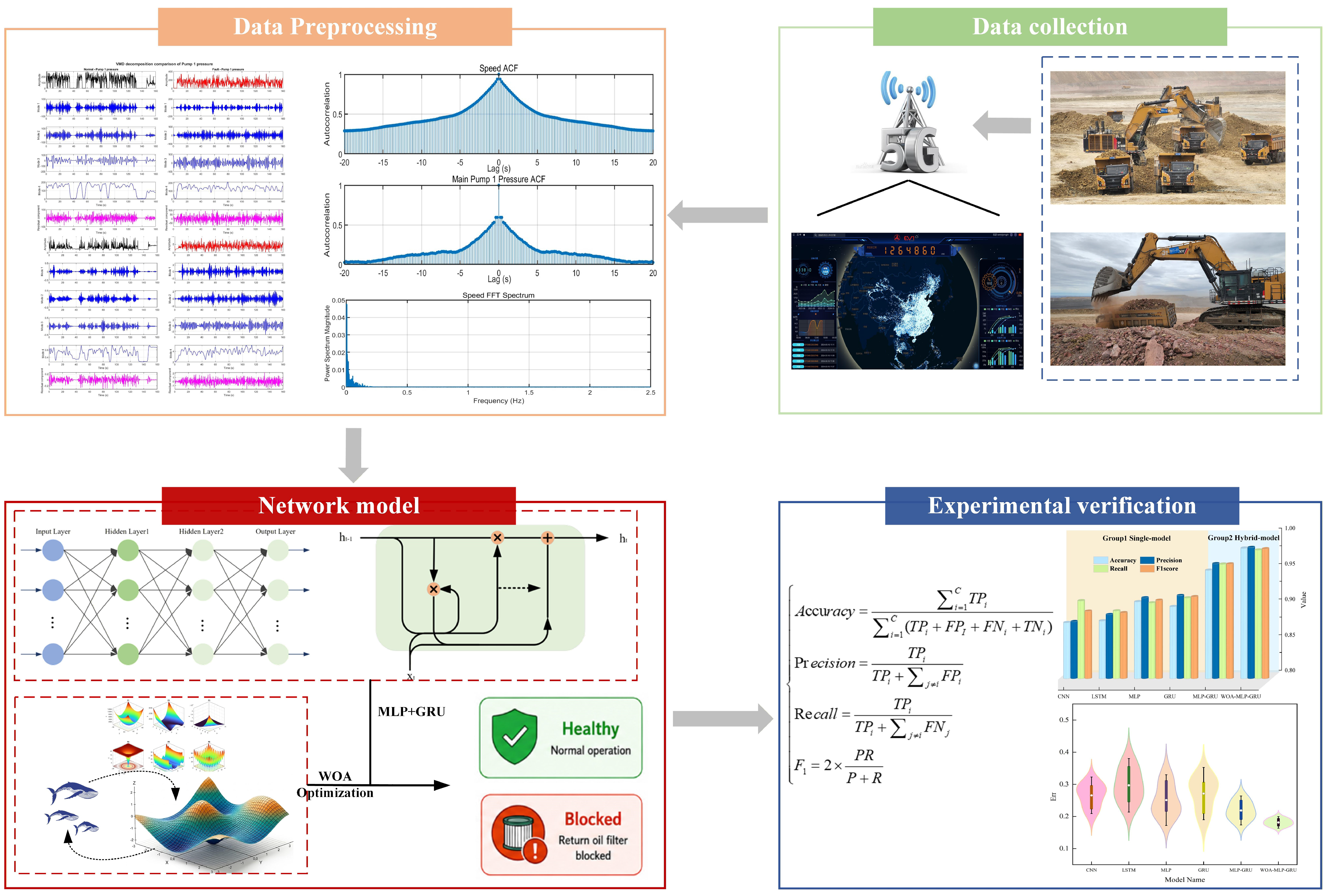
In this study, a SANY SY550 excavator was selected as the research object. Owing to the complex operating conditions, pronounced load fluctuations, and high dimensionality of hydraulic system data, fault identification based on a single MLP or GRU model may be insufficient to fully characterize return oil filter clogging. To address this issue, an MLP-GRU network was constructed, in which the MLP was used to model nonlinear correlations among multi-source input features and the GRU was employed to capture the temporal evolution of fault states. In addition, the whale optimization algorithm (WOA) was introduced to automatically optimize key hyperparameters of the network, thereby reducing the dependence on manual trial-and-error and improving parameter search effectiveness. The overall research framework is shown in Figure 1. The main contributions of this study are summarized as follows.

Figure 1. Overall Framework for Return Oil Filter Diagnosis.

(1)

A WOA-MLP-GRU-based identification framework is proposed for excavator return oil filter clogging faults. By integrating the nonlinear feature coupling capability of MLP, the temporal dependency modeling ability of GRU, and the hyperparameter optimization capability of WOA, the proposed model improves the identification performance for clogging faults under complex operating conditions.

(2)

Considering the complex operating conditions of excavators and the progressive evolution of return oil filter clogging, a mechanism-driven variable selection strategy was adopted to identify representative inputs from pressure, temperature, and operating-condition signals. Furthermore, ACF and FFT analyses were used to support signal denoising, and VMD was introduced to analyze representative pressure signals at the modal level, thereby providing additional physical evidence for fault evolution and the rationality of the selected variables.

(3)

In combination with the working characteristics of the return oil filter, the identification performance of the proposed model was validated under common excavation operations. Using 20 Hz cloud data collected from the SY550 excavator as input, the proposed method was compared with five widely used models through multiple evaluation metrics.

The remainder of this paper is organized as follows. Section 2 introduces the composition of the excavator hydraulic system and the data preprocessing procedure. Section 3 presents the performance evaluation of the WOA algorithm and the corresponding optimization process. Section 4 describes the proposed WOA-MLP-GRU identification model. Section 5 introduces the evaluation metrics and the related experiments.

2. Components of an Excavator’s Hydraulic System and Data Processing

2.1. Components of a Hydraulic System

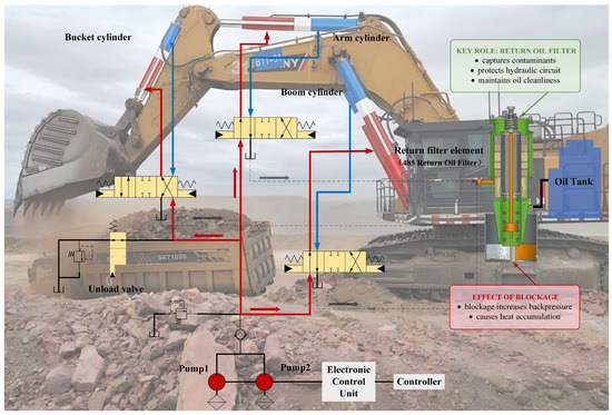
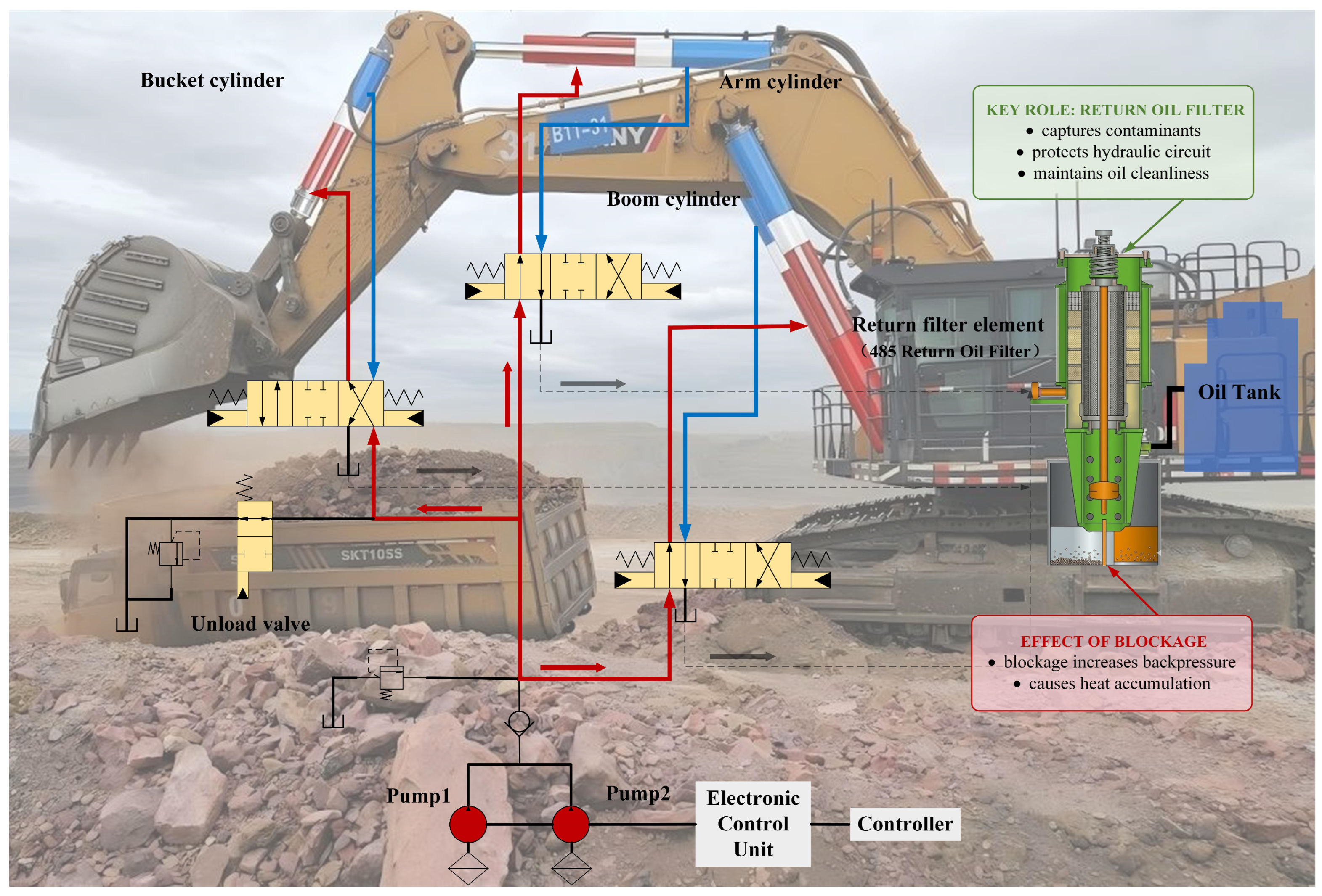
The excavator hydraulic system mainly consists of a power unit, a control unit, an actuation unit, an oil circuit, and a filtration and protection unit, which work together to accomplish the operating process, as shown in Figure 2. The power unit mainly includes the hydraulic pump, which converts the mechanical energy output from the engine into hydraulic energy and provides pressurized oil for the actuators. The control unit primarily comprises the electronic control unit, controllers, and multi-way directional valves, and is responsible for command transmission, valve regulation, and coordinated system control. The actuation unit consists of the boom cylinder, arm cylinder, and bucket cylinder, which convert hydraulic energy into mechanical output to realize different operating motions [22,23]. The return oil filter is arranged in the return branch of the system to maintain hydraulic oil cleanliness and ensure smooth return flow.

Figure 2. Components of an Excavator’s Hydraulic System.

2.2. Data Collection

The SANY SY550 hydraulic excavators (Sany Heavy Machinery SY550 model excavator, manufacturer: Sany Heavy Machinery, Kunshan, Suzhou, China) used in this study have an operating weight of 55,000 kg, a rated power of 310 kW, and a rated speed of 1800 rpm. The detailed equipment specifications are listed in Table 1.

Table 1. Key Technical Specifications of Excavators.

Equipment	Type	Main Parameters
Excavator	SY550	Total weight 55000 kg, 310 KW, 1800 rpm
Return Oil Filter	485 Return Oil Filter	β10(c) ≥ 10, −30 to +100 °C, 18,000 cm2
Displacement sensor	SH30-2000-V2	Scale 0~2000 mm
Pressure sensor	GPTJG3YG400BS CHX	4~20 mA, 2.5 XFS, 5 XFS
Temperature sensors	HST-PM6	−40~150 °C, 4–20 mA
USB-CAN card	USBCAN-II Pro	50–8000 kbps
Controller	BODAS RC28-14/30	4 CAN bus, 4, 32-bit CPU
Graphics card	NVIDIA GeForce	RTX3090
CPU	Intel	Intel Core i9-12900H CPU
Software environment	MATLAB	R2024a

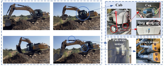
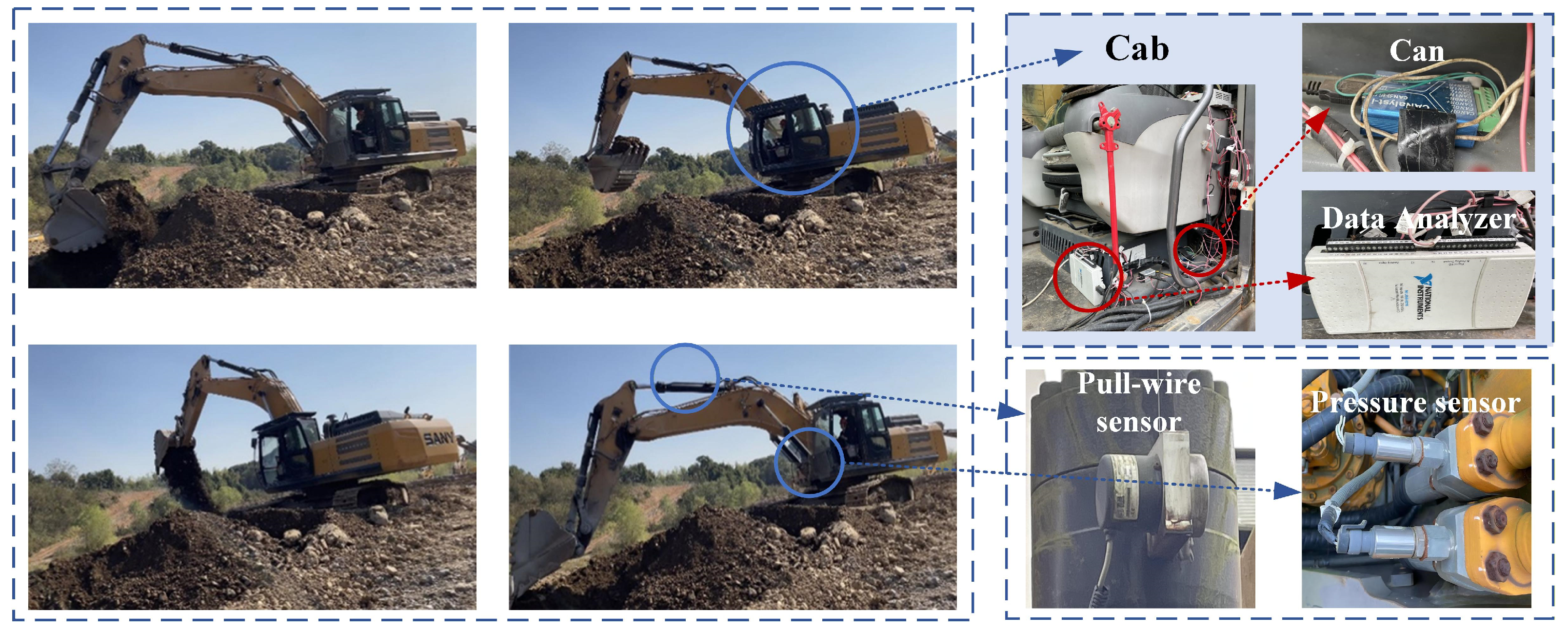
An SH30-2000-V2 draw-wire displacement sensor was installed on the cylinders of the excavator working device to measure cylinder extension and retraction displacement. GPTJG3YG400BS-CHX pressure sensors were arranged at key hydraulic pressure points to collect pressure data from the main hydraulic circuit and the return circuit. In addition, an HST-PM6 temperature sensor was installed in the hydraulic oil tank to monitor hydraulic oil temperature. All sensor signals were transmitted to the BODAS RC28-14/30 controller for unified data acquisition and processing, and then uploaded to the EVI cloud platform via the CAN bus and the USBCAN-II Pro module. The typical operating process and data acquisition procedure were analyzed. As shown in Figure 3, a complete excavator operating cycle generally lasts about 12–15 s and usually consists of four stages: excavation, slewing, unloading, and resetting. Because different operating stages correspond to different load levels and hydraulic system states, the parameters in the hydraulic circuit can, to a certain extent, characterize the system condition and fault evolution process.

Figure 3. Excavator Work Cycle.

The experimental data were collected from ten SANY SY550 excavators at the Kunshan test site in Jiangsu Province, including machines such as SY055BCD30608 and SY0555CC32058. These excavators were selected based on historical maintenance and alarm records containing repeated return-oil-filter clogging events. Multi-source hydraulic and operating parameters were continuously collected by onboard sensors and uploaded to the SANY EVI cloud platform at a sampling frequency of 20 Hz. Approximately 640,000 groups of normal and fault samples were obtained. To reduce the risk of information leakage, the dataset was partitioned by excavator serial number rather than by randomly splitting individual samples. Of the ten excavators, data from seven machines were used for model development, while the remaining three excavators were reserved exclusively for final independent testing. Within the seven development excavators, five machines were used for model training and the other two were used for validation and hyperparameter tuning. Therefore, samples from the same excavator or operating cycle did not appear simultaneously in the training, validation, and test sets. This machine-wise partitioning strategy provides a more reliable assessment of the model’s cross-machine generalization capability under real operating conditions.

2.3. Fault Analysis of the Return Oil Filter

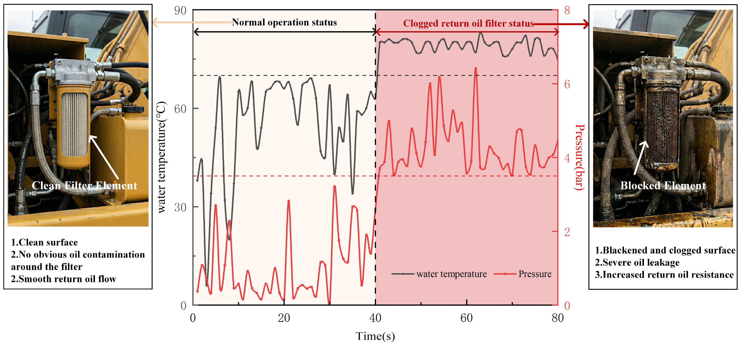
The return-oil filter removes impurities from the hydraulic oil and prevents contaminants from re-entering the hydraulic system. As shown in Figure 4, evident changes can be observed in the filter element before and after clogging. With continued operation, contaminant particles are progressively retained within the filter pores, resulting in narrowed flow passages and increased hydraulic resistance. This, in turn, leads to an increase in return-oil pressure and promotes heat accumulation, thereby disturbing the thermal balance of the system. Therefore, filter clogging is a progressive fault rather than an instantaneous event, and its development is accompanied by continuous changes in both hydraulic resistance and thermal response. During actual excavator operation, however, external vibration and impact may also be transmitted to valves, sensors, fittings, and filter components. As a result, valve-element oscillation, pressure pulsation, cavitation, and hydraulic or structural resonance may induce transient pressure responses that resemble those caused by clogging. In addition, hose deformation or bending, variations in the effective internal flow area, local restrictions at fittings, and other pipeline abnormalities may increase local hydraulic resistance and consequently affect both return-oil pressure and temperature. Therefore, filter clogging cannot be identified reliably from a single instantaneous pressure measurement. In this study, pressure, temperature, and other operating variables are jointly analyzed. VMD is further employed to separate pressure variations with different temporal characteristics, thereby distinguishing slowly varying degradation-related trends from short-term fluctuations within the monitored frequency range. All signals are sampled at 20 Hz, which is intended to capture the relatively slow evolution of clogging-related operating-state characteristics rather than to characterize individual high-frequency vibration modes [24,25,26,27].

Figure 4. Characteristics of the Return Oil Filter in Normal and Faulty Conditions.

However, under practical operating conditions, return-oil-filter clogging cannot be reliably identified from a single pressure signal because load fluctuations, oil-viscosity changes, cold starts, and transient disturbances may also cause temporary pressure increases. Therefore, the binary normal/clogged labels in this study were determined by combining after-sales maintenance records, confirmed filter-replacement information, and laboratory verification of recovered filters. Historical operating data before confirmed clogging events were further traced to characterize the transition from normal operation to clogging. Laboratory tests showed that clogged filters generally exhibited a sustained abnormal pressure response of approximately 4.5 bar. As shown in Figure 4, coolant temperature and return-oil pressure also show relatively clear separation around 70 °C and 4.5 bar, respectively; however, these values were used only as auxiliary physical references rather than universal classification thresholds. Since filter clogging is a progressive fault with clear temporal evolution, reliable identification requires the joint analysis of multidimensional operating variables and their temporal characteristics.

2.4. Key Input Variable Selection and VMD Analysis of Pressure Signals

Based on the above fault-mechanism analysis and the measurable data available from the SANY EVI cloud platform, 16 candidate variables were first considered from the perspectives of pressure, temperature, and operating conditions, as listed in Table 2. The final input variables, however, were not determined solely by data availability, but by their physical relevance to the clogging mechanism and their ability to characterize the propagation of the fault from local flow-resistance abnormality to system-level thermo-hydraulic response. Accordingly, seven variables were retained as model inputs. Among them, return oil filter pressure is the most sensitive core variable because it directly reflects the increase in return-flow resistance and local pressure loss caused by clogging. Pump 1 pressure and pump 2 pressure characterize the pressure response transferred from elevated return backpressure to the pump side, whereas water temperature and hydraulic oil temperature describe the thermal-state evolution associated with increased throttling loss and heat accumulation.

Table 2. Feature Variables.

Candidate Feature	Name	Input Features	Name
X1	Gear position	X2	Engine speed
X2	Engine speed	X3	Pump 1 pressure
X3	Pump 1 pressure	X4	Pump 2 pressure
X4	Pump 2 pressure	X7	Water temperature
X5	Atmospheric pressure	X8	Hydraulic oil temperature
X6	Real-time fuel consumption	X9	Engine oil pressure
X7	Water temperature	X11	Return oil filter pressure
X8	Hydraulic oil temperature
X9	Engine oil pressure
X10	Altitude
X11	Return oil filter pressure
X12	Bucket rodless chamber pressure
X13	Boom rodless chamber pressure
X14	Boom rod chamber pressure
X15	Arm rodless chamber pressure
X16	Arm rod chamber pressure

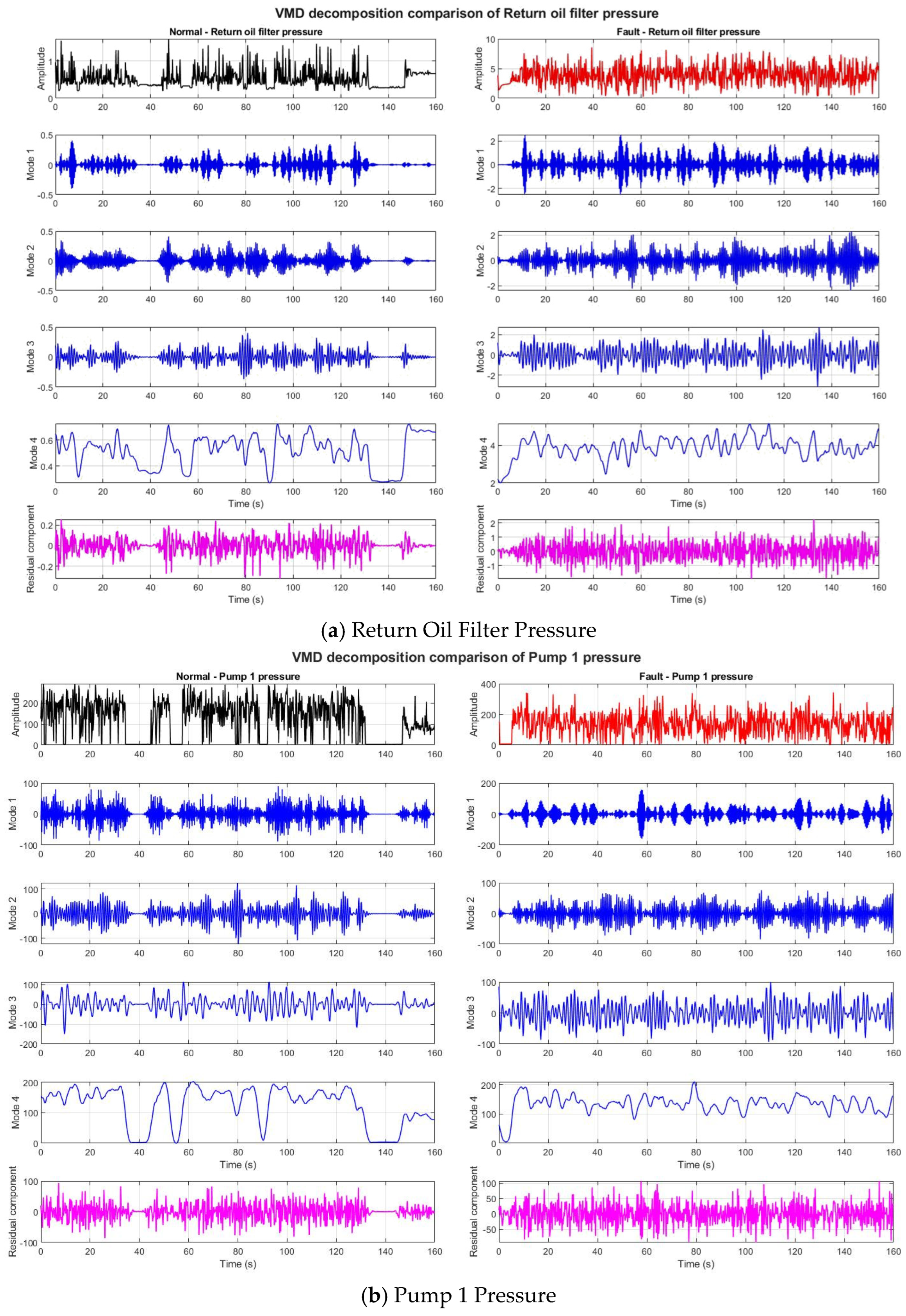
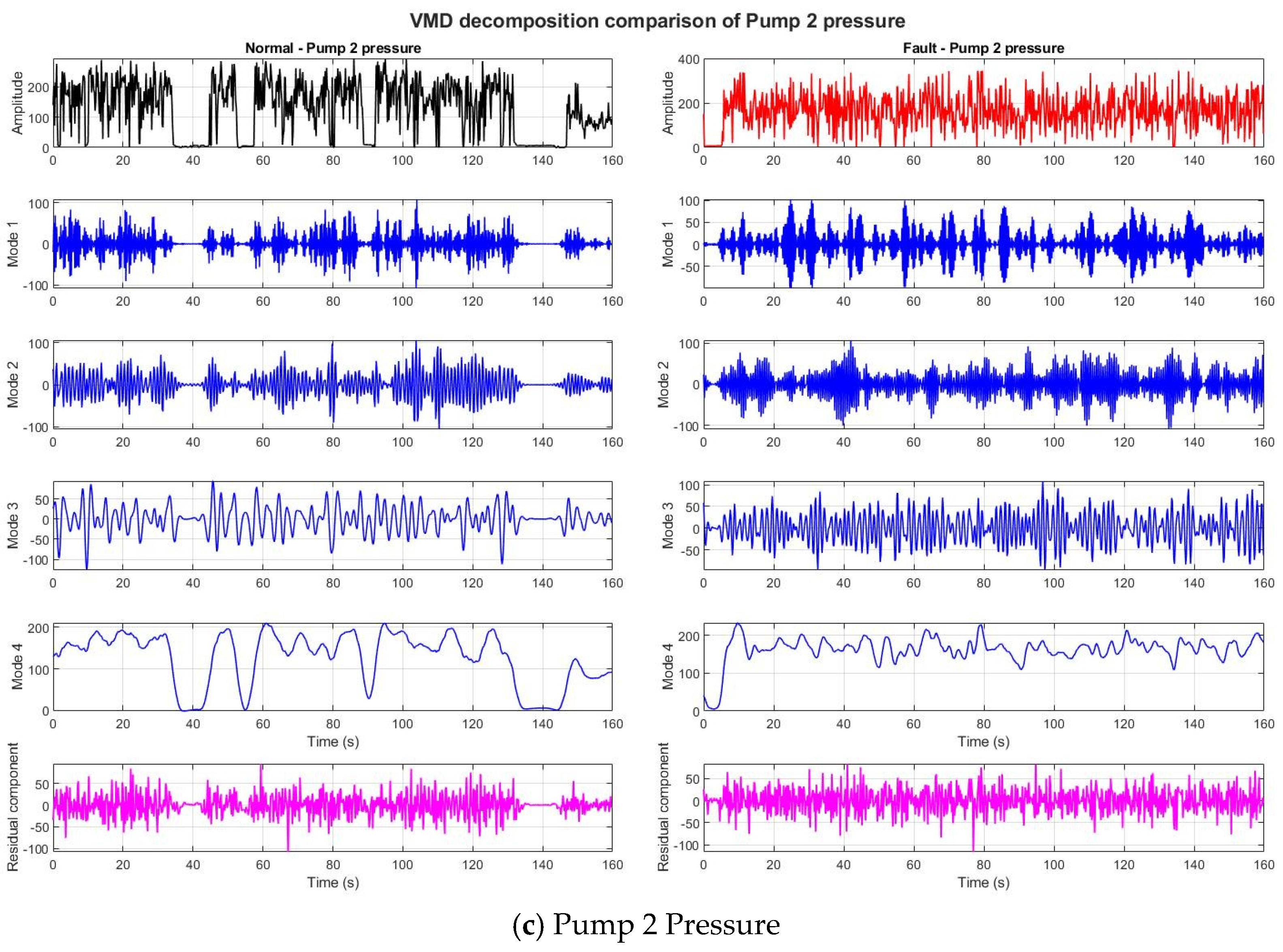
To further verify the mechanism-driven variable selection strategy, supplementary VMD analysis was conducted on three representative pressure variables, including return oil filter pressure (Figure 5a), pump 1 pressure (Figure 5b), and pump 2 pressure (Figure 5c). These variables were selected because they are directly associated with the fault propagation path of return oil filter clogging and can provide representative evidence of pressure response evolution. Other retained variables, such as temperature- and operation-related parameters, mainly reflect thermal effects and external disturbances, which have been justified through mechanism analysis and model validation; therefore, additional VMD analysis was not performed for all variables.

Quantitative evaluation further supports the effectiveness of the selected pressure variables. The return oil filter pressure achieved the highest discrimination capability, with Cohen’s d, Fisher Score, and AUC values of 2.9132, 4.2432, and 0.9867, respectively, indicating a significant difference between normal and clogged conditions. Although pump 1 pressure and pump 2 pressure showed weaker separability, their variations still reflect the propagation of clogging-induced disturbances through the hydraulic system. Furthermore, VMD analysis demonstrated consistent modal changes among the three pressure signals, with energy redistribution values of 0.9819%, 4.2800%, and 0.6759%, respectively, confirming that these variables contain dynamic information related to clogging evolution. Overall, the quantitative results verify the rationality of the proposed mechanism-driven variable selection strategy. The selected variables are supported not only by physical interpretation but also by statistical and time-frequency characteristics, providing reliable inputs for subsequent fault identification.

Figure 5. Variational Mode Decomposition Analysis.

Figure 5. Variational Mode Decomposition Analysis.

2.5. Noise Analysis and Data Standardization

During actual data acquisition, the measured signals are inevitably contaminated by noise due to multiple factors such as harsh operating environments, vibration and impact, and signal transmission media. This may lead to local distortion and measurement errors, thereby adversely affecting the performance of neural network models. Under this circumstance, analyzing the noise characteristics of the raw data is of great significance.

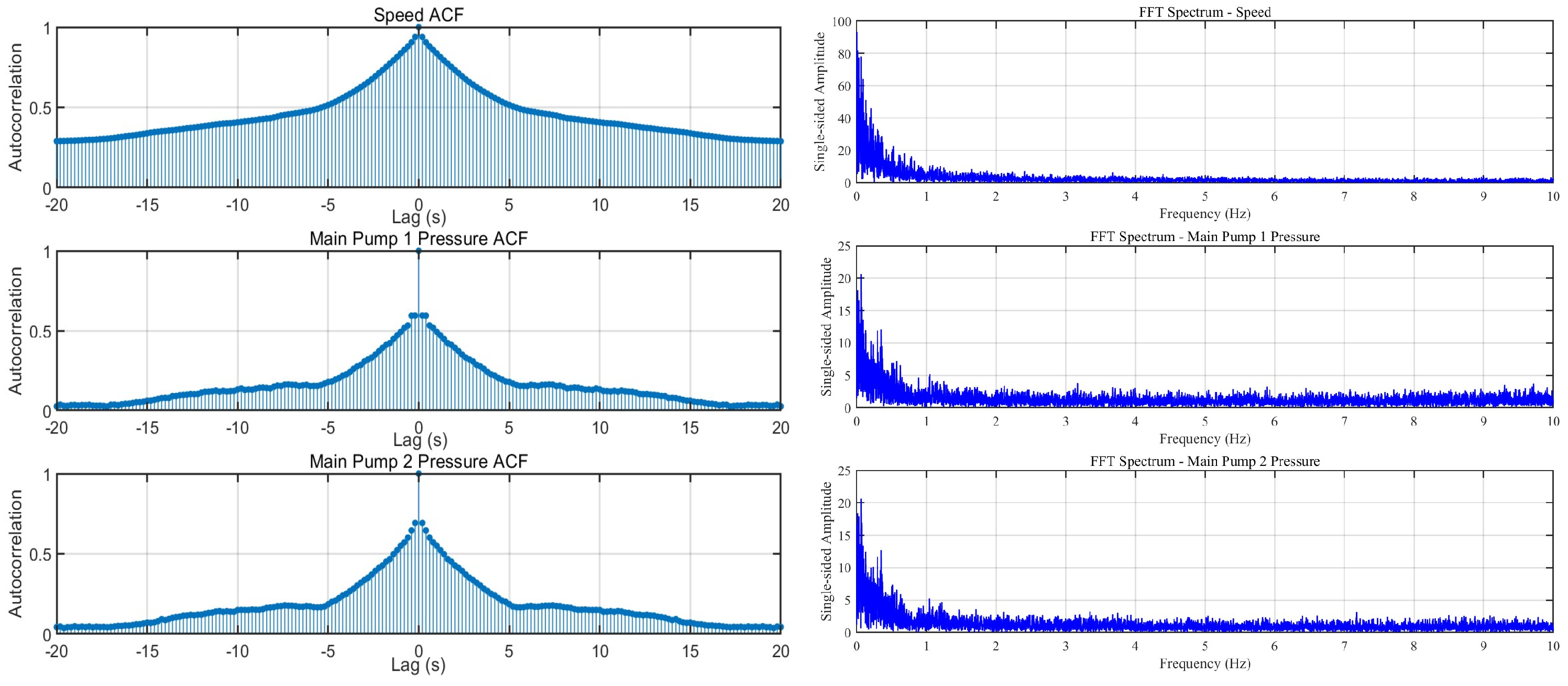
Taking pump pressure and rotational speed data as examples, a joint analysis based on the autocorrelation function (ACF) and fast Fourier transform (FFT) was conducted, and the results are shown in Figure 6. The ACF results indicate that both signals reach their peak at zero lag and then exhibit a clear gradual decay as the lag order increases. The FFT spectra further show that the signal energy is mainly concentrated in the low-frequency region, with pronounced spectral peaks near zero frequency, whereas the energy distribution in the high-frequency range is relatively weak and smooth, without the approximately uniform distribution over a wide frequency band that is typical of white noise [28,29].

Figure 6. ACF Noise Analysis and FFT Analysis.

Based on the temporal and spectral characteristics revealed by the ACF and FFT analyses, a UKF-based filtering method was adopted for signal preprocessing. A two-state model consisting of the signal value and its rate of change was defined as $x_k=\left[x_k,{\dot{x}}_k\right]$. At a sampling frequency of 20 Hz, the sampling interval was ${\mathrm{T}}_{\mathrm{s}}=0.05 \mathrm{s}$, and the state transition and observation models were expressed as:

$$\begin{array}{l}{\mathrm{x}}_{\mathrm{k}+1}=\left[\begin{array}{cc}1& {\mathrm{T}}_{\mathrm{s}}\\ 0& 1\end{array}\right]{\mathrm{x}}_{\mathrm{k}}+{\mathrm{w}}_{\mathrm{k}}\\ {\mathrm{z}}_{\mathrm{k}}=\left[1 0\right]{\mathrm{x}}_{\mathrm{k}}+{\mathrm{v}}_{\mathrm{k}}\end{array}$$

(1)

For each continuous data segment, the initial state was set using the first measurement with zero initial rate of change. The UKF sigma-point parameters were fixed as α = 0.5, β = 2, and κ = 0. The process and measurement noise parameters were selected by jointly considering innovation consistency, innovation characteristics, and filtering smoothness.

The filtered data were further normalized to accelerate the training process and improve model stability. The normalization formula is given as follows:

$${\mathrm{x}}^{\prime }={\displaystyle \frac{\mathrm{x}-{\mathrm{x}}_{\min }}{{\mathrm{x}}_{\max }-{\mathrm{x}}_{\min }}}$$

(2)

In the above equation, x denotes the filtered data, ${\mathrm{x}}_{\min }$ and ${\mathrm{x}}_{\max }$ represent the minimum and maximum values of the filtered data, respectively, and ${\mathrm{x}}^{\prime }$ is the normalized result.

3. Optimization Algorithms

3.1. Whale Optimization Algorithm (WOA)

The whale optimization algorithm (WOA) is an optimization method proposed in 2016 based on the bubble-net feeding behavior of humpback whales. Owing to its simple structure, fast convergence, strong robustness, and balanced capability for global exploration and local exploitation, WOA has been widely used for neural network hyperparameter optimization. The entire optimization process is carried out through three mechanisms: encircling prey, spiral updating, and random search. In nature, when whales fail to locate prey directly, they randomly select a position within the population and perform large-scale area exploration to increase the probability of capture [30,31]. In practical terms, this means that when the optimal solution has not yet been found, the search position is dynamically adjusted to move toward a potentially better solution. The corresponding expression is given as follows:

$$\begin{array}{l}\mathrm{D}=\left|\mathrm{C}\cdot {\mathrm{X}}_{\mathrm{r}\mathrm{a}\mathrm{n}\mathrm{d}}(\mathrm{t})-\mathrm{X}(\mathrm{t})\right|\\ \mathrm{X}(\mathrm{t}+1)={\mathrm{X}}_{\mathrm{r}\mathrm{a}\mathrm{n}\mathrm{d}}(\mathrm{t})-\mathrm{A}\cdot \mathrm{D}\end{array}$$

(3)

In the above equations, $\mathrm{X}(\mathrm{t})$ denotes the position of the current individual at the t-th iteration, ${\mathrm{X}}_{\mathrm{r}\mathrm{a}\mathrm{n}\mathrm{d}}(\mathrm{t})$ represents a randomly selected position, $\mathrm{X}(\mathrm{t}+1)$ is the updated position, D denotes the distance difference between the individual and the population, and A and C are control parameter vectors.

Once the target prey is detected, the search range is gradually reduced to form an encircling behavior. Assuming that the current best position found is ${\overrightarrow{\mathrm{X}}}^{*}(\mathrm{t})$, and that the whale position at the t-th iteration is $\overrightarrow{\mathrm{X}}(\mathrm{t})$, the encircling behavior can be expressed as follows:

$$\begin{array}{l}\overrightarrow{\mathrm{D}}=\left|\overrightarrow{\mathrm{C}}\cdot {\overrightarrow{\mathrm{X}}}^{*}(\mathrm{t})-\overrightarrow{\mathrm{X}}(\mathrm{t})\right|\\ \overrightarrow{\mathrm{X}}(\mathrm{t}+1)={\overrightarrow{\mathrm{X}}}^{*}(\mathrm{t})-\overrightarrow{\mathrm{A}}\cdot \overrightarrow{\mathrm{D}}\end{array}$$

(4)

$$\begin{array}{l}\overrightarrow{A}=2\overrightarrow{a}\cdot \overrightarrow{r}-\overrightarrow{a}\\ \overrightarrow{C}=2\overrightarrow{r}\end{array}$$

(5)

In the above equations, $\overrightarrow{\mathrm{r}}$ is a random variable in the interval [0, 1], $\overrightarrow{\mathrm{a}}$ denotes the convergence factor, and $\overrightarrow{\mathrm{A}},\overrightarrow{\mathrm{C}}$ are coefficient vectors used to control the search behavior.

During prey capture, the whale updates its position through a spiral attacking mechanism. In essence, this means that the individual approaches the target along a spiral trajectory, thereby improving the accuracy of local search. The mathematical expression is given as follows:

$$\overrightarrow{\mathrm{X}}(\mathrm{t}+1)=\overrightarrow{\mathrm{D}}\cdot {\mathrm{e}}^{\mathrm{b}\mathrm{l}}\cdot \cos (2\mathrm{\pi }\mathrm{l})+{\overrightarrow{\mathrm{X}}}^{*}(\mathrm{t})$$

(6)

In the above equation, b denotes the constant defining the spiral shape, and l is a random number within the interval [−1, 1].

3.2. Comparison and Evaluation of Optimization Algorithms

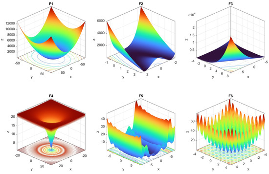
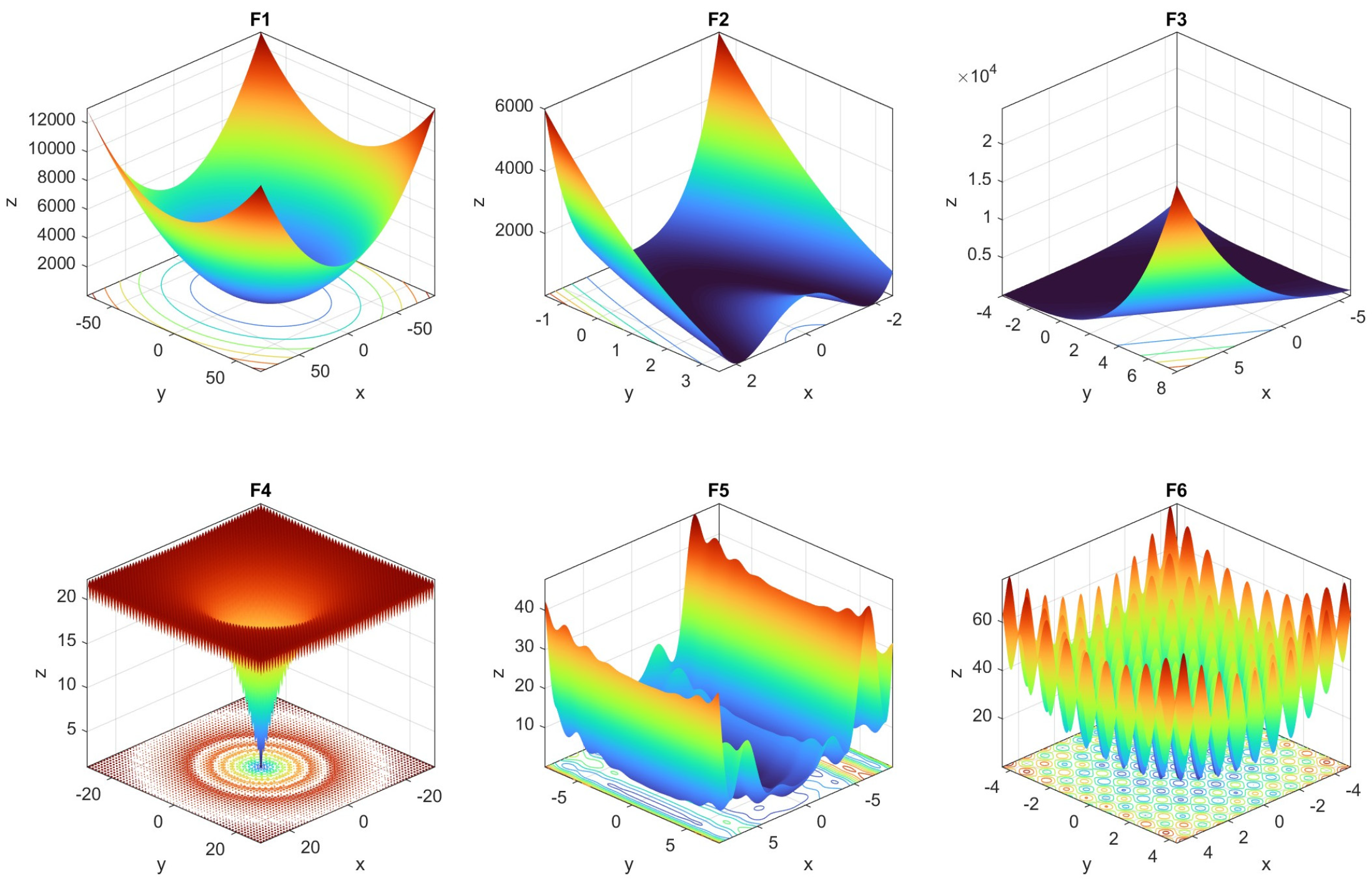
The previous section described the three underlying mechanisms of the WOA algorithm. To further verify its overall advantages, this section evaluates WOA using six benchmark functions and compares its performance with three representative optimization algorithms, namely particle swarm optimization (PSO), the honey badger algorithm (HBA), and Bayesian optimization (BO). Among these benchmark functions, F1~F3 are unimodal functions, whereas F4~F6 are multimodal functions. Figure 7 illustrates the landscapes of the six benchmark functions, and Table 3 summarizes the definition of each function.

Figure 7. Evaluation function curve.

Table 3. Evaluation Functions.

No	Function	Dimension	Range
1	$F_1(x)={\displaystyle {\sum }_{i=1}^n{x}_i^2}$	30	[−50, 50]
2	$\begin{array}{l}{F}_2(x)={{\displaystyle {\sum }_{i=1}^{n-1}\left[100(x_{i+1}-x_i^2)\right.}}^2\\ \left.+{(x_i-1)}^2\right]\end{array}$	30	[−2, 3]
3	$\begin{array}{l}{F}_3(x)={\displaystyle {\sum }_{i=1}^n{x}_i^2}+{({\displaystyle {\sum }_{i=1}^{n}0.5i{x}_i})}^2\\ +{({\displaystyle {\sum }_{i=1}^{n}0.5i{x}_i})}^4\end{array}$	30	[−5, 10]
4	$\begin{array}{l}{F}_4(x)=-20\exp (-0.2\sqrt{{\displaystyle \frac{1}{n}}{\displaystyle {\sum }_{i=1}^n{x}_i^2}})\\ -\exp ({\displaystyle \frac{1}{n}}{\displaystyle {\sum }_{i=1}^n\cos (2\pi x_i)})\\ +20+e\end{array}$	30	[−20, 20]
5	$\begin{array}{l}{F}_5(x)={\sin }^2(\pi {\omega }_1)+{{\displaystyle \sum _{i=1}^{n-1}({\omega }_i-1)}}^2\\ *\left[1+10{\sin }^2(\pi {\omega }_i+1)\right]+\\ {({\omega }_n-1)}^2\left[1+{\sin }^2(2\pi {\omega }_n)\right]\end{array}$	30	[−5, 5]
6	$\begin{array}{l}{F}_6(x)={\displaystyle {\sum }_{i=1}^n\left[x_i^2\right.}-10\cos (2\pi x_i)\\ \left.+10\right]\end{array}$	30	[−4, 4]

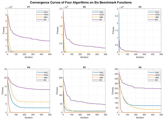
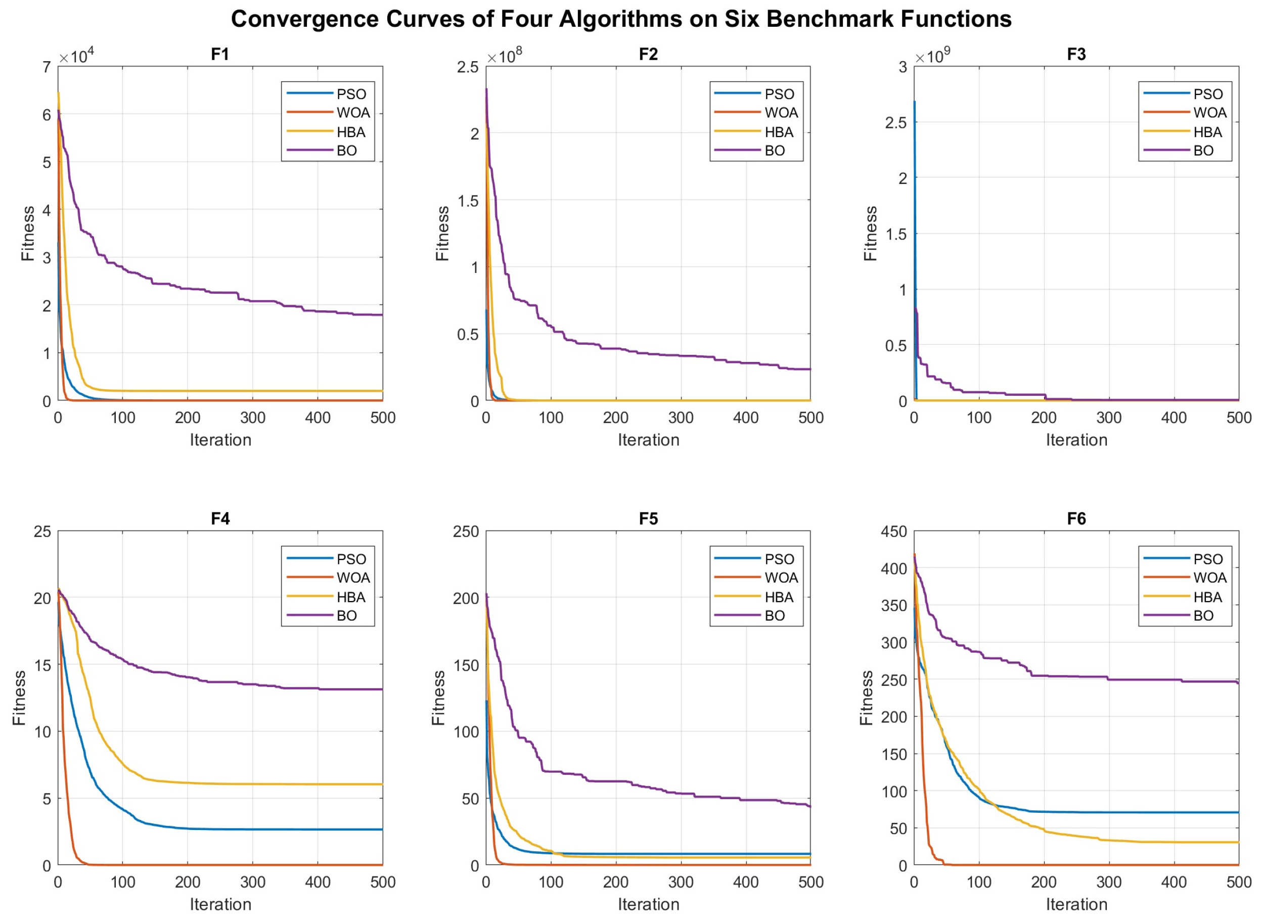
To ensure the reliability of the comparison results, each algorithm was independently executed 100 times on each benchmark function. The performance of the algorithms was evaluated using the mean value, standard deviation, and optimal value, where the mean value was used to measure the overall optimization accuracy, the standard deviation was used to reflect stability and robustness, and the optimal value was adopted to assess the search capability. For all algorithms, the population size was set to 30, the dimensionality was set to 30, and the maximum number of iterations was set to 500. Figure 8 presents the convergence curves of the different optimization algorithms on multiple benchmark functions, and the corresponding performance results are listed in Table 4.

Figure 8. Convergence curves of the four optimization algorithms.

Table 4. Performance Test Results for the Optimization Algorithm.

Function	Algorithm	Mean Value	Standard Deviation	Optimal Solution
F1	PSO	3.0524 × 10−5	5.0209 × 10−5	2.1906 × 10−8
	WOA	1.1491 × 10−85	3.0047 × 10−85	4.9028 × 10−93
	HBA	2000	4216.4	5.5482 × 10−7
	BO	17916	2158.7	15422
F2	PSO	52.176	32.409	4.6084
	WOA	4.1547	8.9271	0.061854
	HBA	368.4	985.59	26.345
	BO	2.3398 × 107	5.7853 × 106	1.4389 × 107
F3	PSO	74.065	52.885	21.337
	WOA	380.23	229.1	7.9029
	HBA	539.71	344	131.13
	BO	4.9604 × 106	4.9584 × 106	1067.4
F4	PSO	2.6555	0.92305	1.6462
	WOA	2.2204 × 10−15	2.5121 × 10−15	4.4409 × 10−16
	HBA	6.0315	7.8607	0.00036466
	BO	13.125	0.41719	12.512
F5	PSO	8.3001	5.5324	3.4513
	WOA	0.028015	0.040957	0.0001365
	HBA	5.5717	16.866	0.11543
	BO	43.653	8.9552	29.298
F6	PSO	70.749	29.796	30.844
	WOA	0	0	0
	HBA	30.617	18.36	2.5552
	BO	244.44	18.913	215.67

As shown in Figure 8, WOA exhibits a faster convergence rate and achieves lower final fitness values on most benchmark functions, indicating that it can rapidly locate promising regions during the search process while maintaining favorable convergence efficiency. The results in Table 4 further demonstrate that, for F2, F4, F5, and F6, WOA outperforms the other comparative algorithms in terms of mean value, standard deviation, and optimal value. For F3, although the mean value and standard deviation of WOA are slightly inferior to those of PSO, its optimal value still remains superior, suggesting that WOA retains strong global optimization capability on this function. Overall, WOA shows better comprehensive performance on most benchmark functions and is therefore selected as the hyperparameter optimization algorithm for the proposed model.

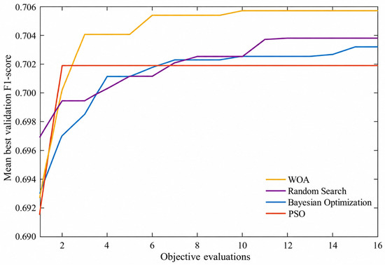
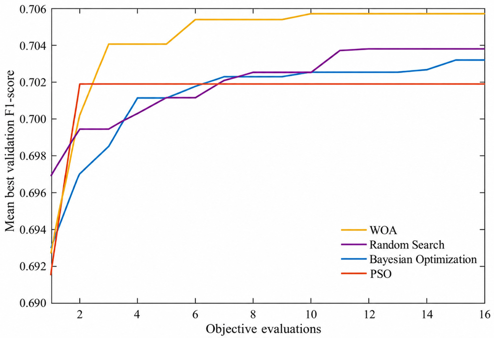
To further verify the applicability of WOA to the proposed model, an equal-budget hyperparameter optimization experiment was conducted for MLP-GRU. WOA, PSO, BO, and RS were compared under the same dataset, search space, and 16 objective evaluations, with validation F1-score as the optimization objective. As shown in Figure 9, WOA achieves faster improvement in the early stage and maintains the highest optimization performance. The mean best validation F1-scores of WOA, RS, BO, and PSO are 0.70572, 0.70374, 0.70313, and 0.70188, respectively. These results demonstrate that WOA provides better optimization efficiency and stability for MLP-GRU hyperparameter tuning.

Figure 9. Performance comparison of different optimization algorithms under equal computational budgets.

3.3. WOA Hyperparameter Optimization

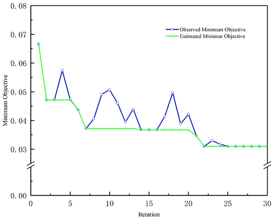
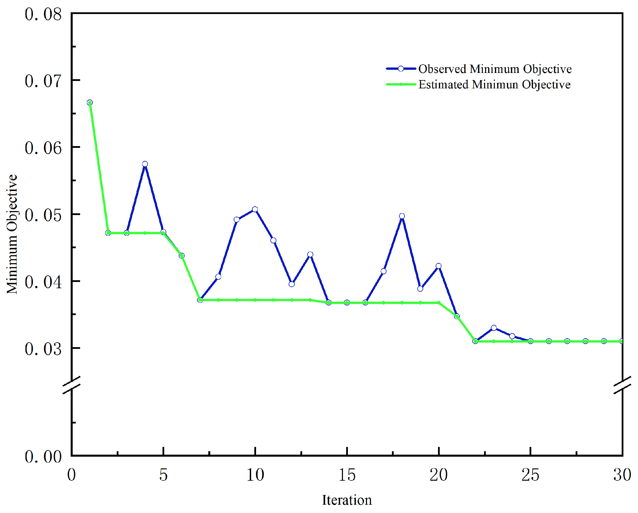
WOA exhibits notable overall advantages in terms of convergence speed, optimization accuracy, and stability, indicating that it can effectively balance global exploration and local exploitation. Therefore, WOA was selected to perform automatic hyperparameter optimization for the proposed model. The hyperparameter optimization process is illustrated in Figure 10. The horizontal axis represents the number of iterations, while the vertical axis denotes the minimum objective function value. The blue curve indicates the best objective value actually observed at each iteration, whereas the green curve represents the estimated best objective value. In this study, the maximum number of iterations was set to 30. On the one hand, for a medium-scale hyperparameter search space, 20–30 iterations generally provide a better trade-off between search adequacy and computational cost. On the other hand, this setting is also consistent with the convergence behavior shown in the figure.

Figure 10. The WOA Optimization Process.

In the early stage, the objective function value decreases rapidly from approximately 0.067 to around 0.047, indicating that WOA can quickly locate a promising hyperparameter region within a limited number of iterations and thus demonstrates strong global search capability. Around the 7th iteration, the objective function value further declines to approximately 0.037, suggesting that the algorithm has entered a more favorable search space. Although the blue curve exhibits some fluctuations between the 8th and 20th iterations, the green curve remains relatively stable overall, indicating that the algorithm at this stage mainly performs local exploration and repeated comparison around the potential optimum region rather than undergoing unstable search behavior. Around the 21st to 22nd iterations, the objective function value decreases again significantly and stabilizes at approximately 0.031. Thereafter, the two curves become nearly coincident with only negligible variation, indicating that the algorithm has converged to a relatively optimal hyperparameter combination. Within the 30 iterations shown in the figure, the objective function decreases to a stable value, and further optimization would yield only limited improvement while incurring additional computational cost. Therefore, 30 iterations is considered appropriate for the hyperparameter optimization task in this study. Overall, the optimization process exhibits the typical pattern of “rapid decline in the early stage, local fluctuating search in the middle stage, and stable convergence in the later stage,” which is consistent with the WOA mechanism of global exploration followed by local exploitation. The optimal hyperparameter results are listed in Table 5.

Table 5. Hyperparameter Optimization Ranges and Results.

Hyperparameters	Range	Optimal Value
Number of hidden cells	[16, 128]	34, 48
Dropout	[0.05, 0.5]	0.1
Learning rate	[1 × 10−4, 1 × 10−2]	0.00066
Weight decay	[1 × 10−6, 1 × 10−3]	5 × 10−5

4. GRU-MLP

4.1. MLP Model

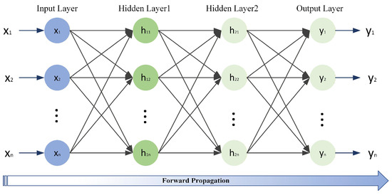
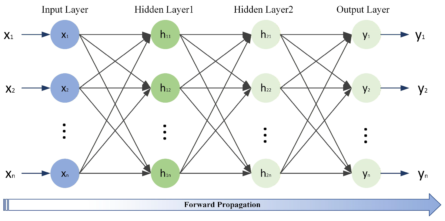
The multilayer perceptron (MLP), as a core model in deep learning, is a feedforward neural network composed of an input layer, one or more hidden layers, and an output layer. By mimicking the structure of biological neurons, the MLP learns the nonlinear relationship between inputs and outputs through layer-by-layer mapping. Moreover, by introducing activation functions into the hidden layers, it achieves strong nonlinear fitting capability [32]. Figure 11 illustrates the architecture of the MLP neural network, and its underlying process can be described as follows:

Figure 11. MLP Architecture Diagram.

In classification tasks, the input features are first subjected to weighted mapping and nonlinear transformation through the hidden layers. The forward propagation process can be expressed as follows:

$$a^{(l)}=f(W^{(l)}{a}^{(l-1)}+b^{(l)})$$

(7)

In the above equation, $a^{(l-1)}$ and $a^{(l)}$ denote the outputs of the (l-1)-th and l-th layers, respectively; $W^{(l)},b^{(l)}$ represent the weight matrix and bias vector of the l-th layer; and $f(\cdot )$ is the activation function. After feature extraction through the hidden layers, the output layer maps the result to the predicted probability of belonging to the positive class via the Sigmoid function, which can be expressed as follows:

$$\widehat{y}=\sigma (z)={\displaystyle \frac{1}{1+e^{-z}}}$$

(8)

In the above equation, z denotes the linear output, $\sigma (\cdot )$ represents the Sigmoid activation function, and $\widehat{y}$ is the predicted probability of the sample. The network employs the binary cross-entropy loss function, which is expressed as follows:

$$L=-{\displaystyle \frac{1}{N}}{\displaystyle \sum _{i=1}^N\left[y_i\log {\widehat{y}}_i+(1-y_i)\log (1-{\widehat{y}}_i)\right]}$$

(9)

In the above equation, L denotes the loss value, N represents the number of samples, and $y_i$ denotes the label of the I-th sample. In this study, the proposed MLP module consists of fully connected layers combined with ReLU activation functions and contains two hidden layers, each with 34 hidden units.

4.2. GRU Model

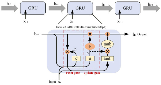
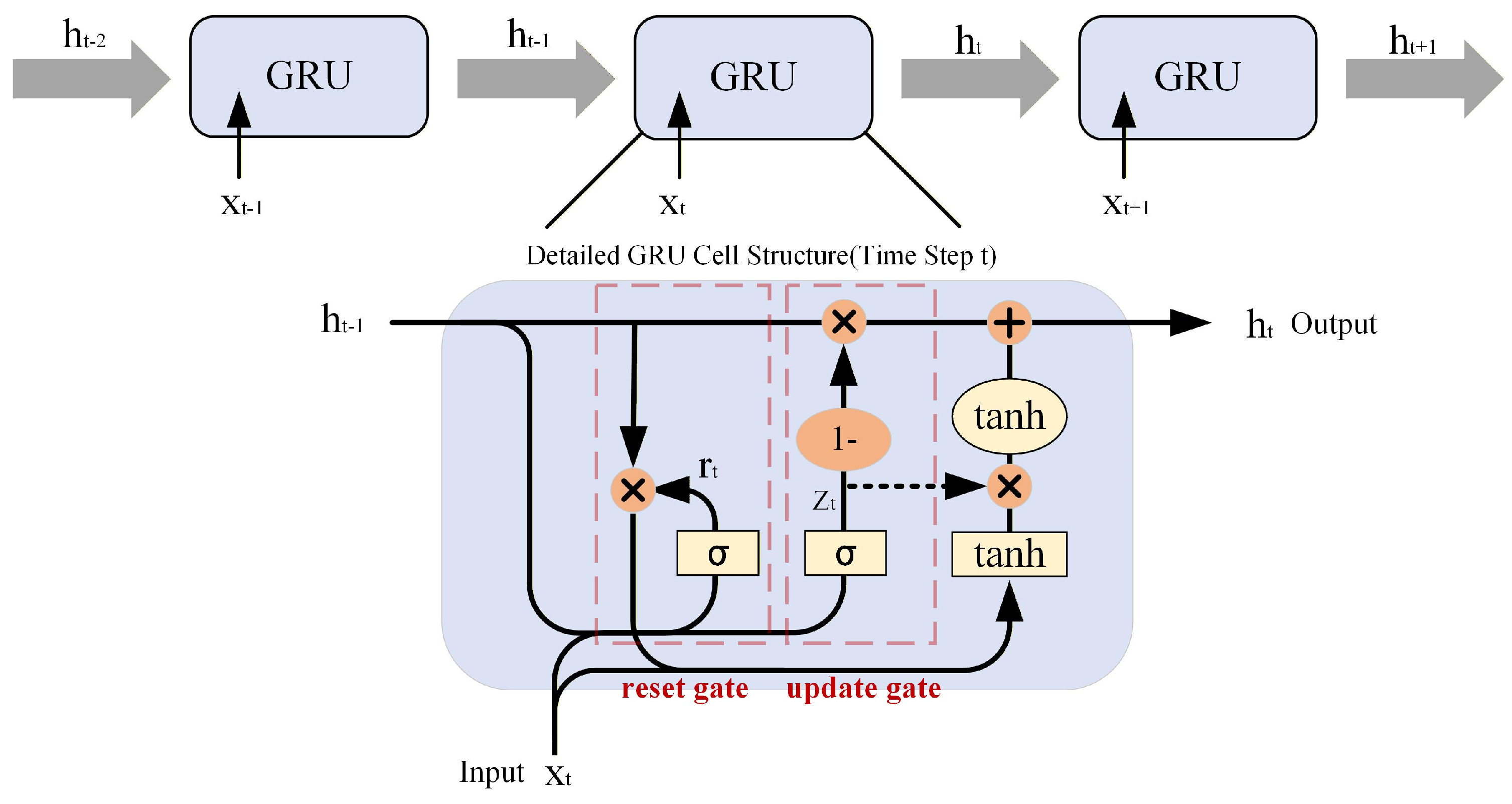
The gated recurrent unit (GRU) is an efficient recurrent neural network designed to address the gradient vanishing problem in traditional RNNs. By introducing a gating mechanism, the GRU employs an update gate and a reset gate to regulate the flow of information, while maintaining a simpler structure and fewer parameters than the long short-term memory (LSTM) network. Figure 12 presents the architecture of the GRU network. Specifically, the GRU first computes the reset gate and update gate based on the current input and the previous hidden state. The reset gate is then used to generate the candidate hidden state, and finally the update gate fuses the historical state with the candidate state through a weighted updating scheme to produce the current hidden state [33,34].

$$\left\{\begin{array}{l}{r}_t=\sigma (W_r{x}_t+U_r{h}_{t-1}+b_r)\\ z_t=\sigma (W_z{x}_t+U_z{h}_{t-1}+b_z)\\ {\tilde{h}}_t=\tanh (W_h{x}_t+U_h(r_t\odot h_{t-1})+b_h)\\ h_t=z_t\odot h_{t-1}+(1-z_t)\odot {\tilde{h}}_t\end{array}\right.$$

(10)

Figure 12. GRU Architecture Diagram.

In the above equations, $x_t$ denotes the current input, $h_{t-1}$ represents the hidden state at the previous time step, $r_t$ and $z_t$ are the reset gate and update gate, respectively, ${\tilde{h}}_t$ denotes the candidate hidden state, and $h_t$ is the current hidden state. In this study, the final hidden representation of the GRU was obtained using the last-output strategy, and the optimal number of hidden units in the GRU was determined to be 48.

4.3. WOA-MLP+GRU Model

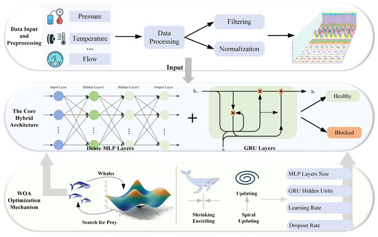
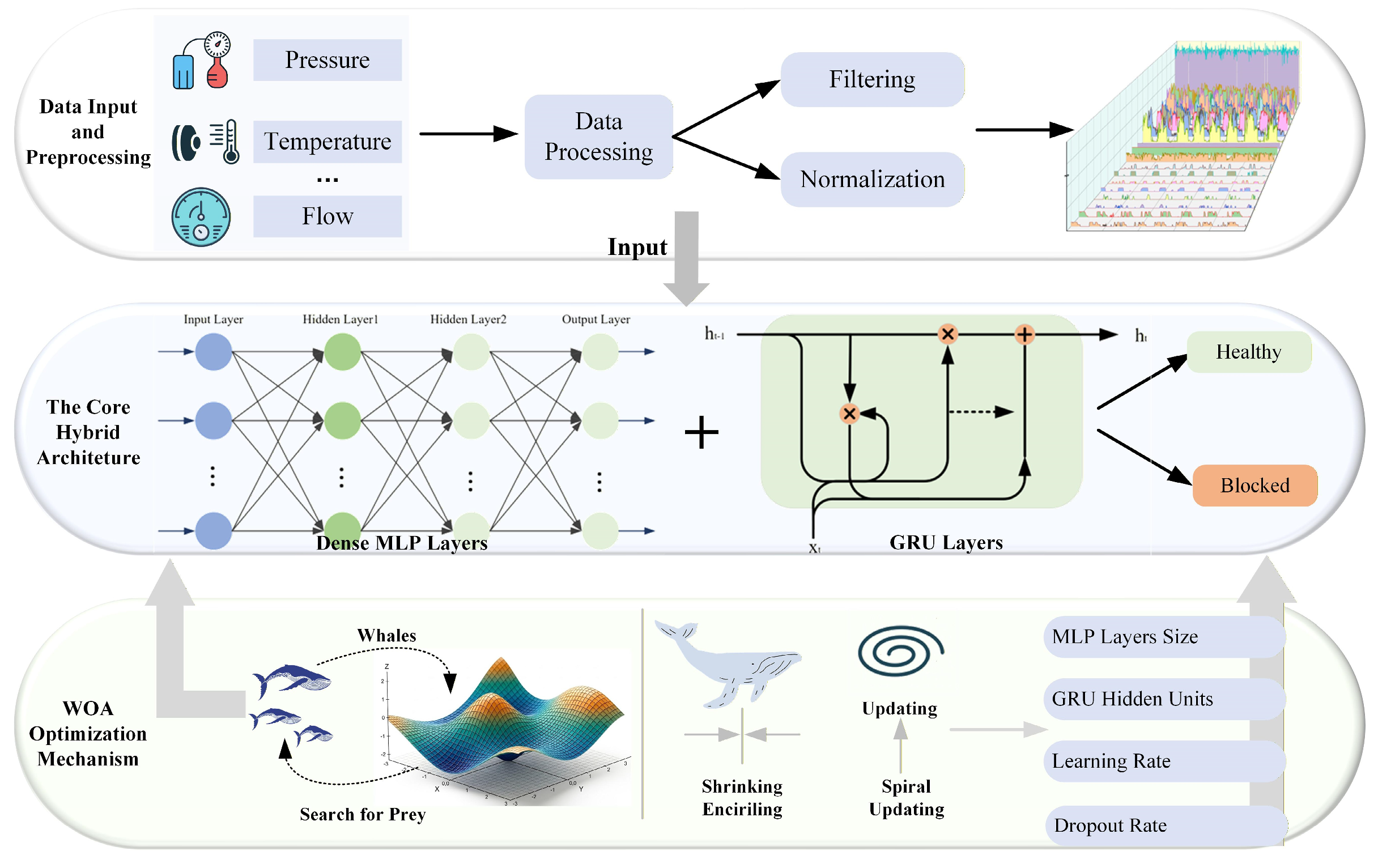
Figure 13 shows the overall architecture of the proposed WOA-MLP-GRU model, which consists of three parts: a data input and preprocessing module, a hybrid identification network, and a WOA-based optimization module. Multi-source signals, such as pressure and temperature, are collected through sensors and the CAN module and then retrieved from the EVI cloud platform. To reduce the influence of noise and fluctuations, the raw data are filtered and normalized before being used as model inputs.

Figure 13. Diagram of the WOA-MLP-GRU framework.

The preprocessed data are first fed into the MLP to perform nonlinear mapping and feature fusion of multidimensional inputs. The extracted features are then sent to the GRU, which captures temporal dependencies and dynamic fault evolution, thereby improving the identification of the transition from the healthy state to the blocked state. Finally, the model outputs the identification result.

To avoid the subjectivity of manual hyperparameter tuning, WOA is introduced to optimize the key parameters of the MLP-GRU model. By iteratively searching the hyperparameter space with the validation-set objective value as the fitness criterion, WOA determines the optimal parameter combination, including the MLP layer size, the number of GRU hidden units, the learning rate, and the dropout ratio, thereby further improving the identification performance of the model.

5. Experimental Results and Analysis

To validate the effectiveness of the proposed WOA-MLP-GRU model for excavator return oil filter clogging fault identification, this chapter conducts experimental analysis on the constructed dataset from four aspects: model performance, convergence behavior, feature representation capability, and output stability. Based on the comprehensive evaluation of model comparisons, training-process analysis, feature separability visualization, and repeated-experiment error distributions, the proposed model is shown to achieve the best overall identification performance under the current dataset and experimental settings, confirming the positive contribution of the hybrid architecture and the WOA-based hyperparameter optimization strategy.

5.1. Evaluation Criteria

To comprehensively evaluate the classification performance of the model, accuracy, precision, recall, and F1-score were selected as the primary evaluation metrics. Among them, accuracy is used to measure the overall correctness of classification; precision reflects the proportion of truly positive samples among those predicted as positive; recall measures the model’s ability to correctly identify positive samples; and the F1-score represents the balance between precision and recall. The calculation formulas of these four metrics are given as follows:

$$\begin{array}{l}\left\{\begin{array}{l}A\mathrm{ccu}racy={\displaystyle \frac{{\displaystyle {\sum }_{i=1}^{C}T{P}_i}}{{\displaystyle {\sum }_{i=1}^C(T{P}_i+F{P}_I+F{N}_i+T{N}_i)}}}\\ \mathrm{Pr}ecision={\displaystyle \frac{T{P}_i}{T{P}_i+{\displaystyle {\sum }_{j\ne i}F{P}_i}}}\\ \mathrm{Re}call={\displaystyle \frac{T{P}_i}{T{P}_i+{\displaystyle {\sum }_{j\ne i}F{N}_j}}}\\ F_1=2\times {\displaystyle \frac{PR}{P+R}}\end{array}\right.\end{array}$$

(11)

In the above equations, $T{P}_{\mathrm{i}}$ denotes the number of samples correctly predicted as class i, $F{P}_{\mathrm{i}}$ denotes the number of samples incorrectly predicted as class i, $F{N}_{\mathrm{i}}$ represents the number of samples incorrectly predicted as non-i, and $T{N}_{\mathrm{i}}$ denotes the number of samples correctly predicted as non-i. The closer these four metrics are to 1, the better the model performance; conversely, values closer to 0 indicate poorer identification performance.

5.2. Model Performance Analysis

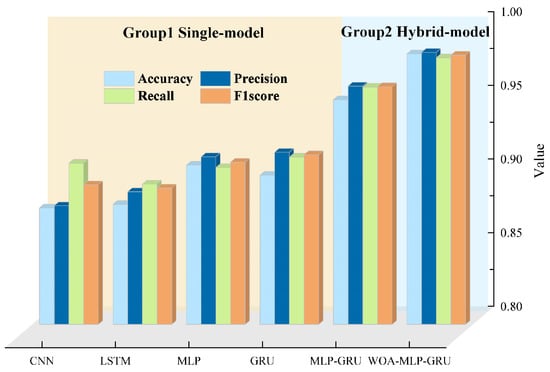
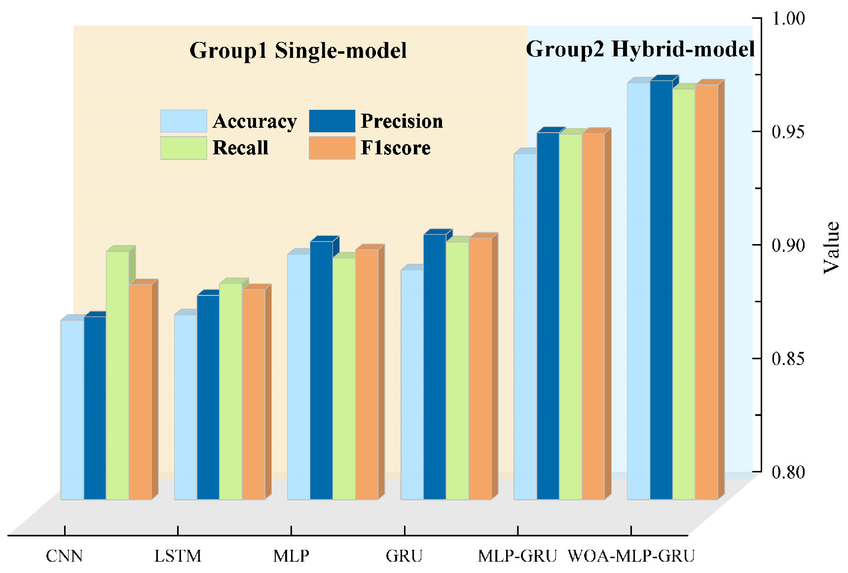
To compare the overall performance of the models from the perspective of the four evaluation metrics, MLP, GRU, MLP-GRU, CNN, and LSTM were selected as comparison models for experiments against the proposed WOA-MLP-GRU model. Their performance in terms of Accuracy, Precision, Recall, and F1-score was statistically analyzed, and the results are presented in Figure 14 and Table 6.

Figure 14. Model Performance Comparison Chart.

Table 6. Evaluation Results.

Model	Accuracy	Precision	Recall	F1-Score
CNN	0.8791	0.8806	0.9094	0.8948
LSTM	0.8815	0.8901	0.8952	0.8926
MLP	0.9081	0.9138	0.9065	0.9101
GRU	0.9012	0.9169	0.9135	0.9152
MLP-GRU	0.9525	0.9618	0.9611	0.9614
WOA-MLP-GRU	0.9836	0.9847	0.9811	0.9828

As shown in Figure 14 and Table 6, CNN and LSTM exhibit comparatively weaker performance among the evaluated models, with classification accuracies below 0.90. Although CNN achieves a Recall of 0.9094, its lower overall performance indicates that a portion of normal samples may be incorrectly classified as clogging faults. MLP and GRU provide more competitive results, with accuracies close to 0.90. In particular, GRU yields higher Precision, Recall, and F1-score than MLP, suggesting that both nonlinear feature interactions and temporal dependencies contribute substantially to the discrimination of filter clogging states. The hybrid MLP-GRU model further improves the four evaluation metrics to 0.9525, 0.9618, 0.9611, and 0.9614, respectively. Compared with MLP and GRU, the corresponding classification error rate is reduced by 48.3% and 51.9%. Moreover, the difference between Precision and Recall is only 0.0007, indicating a more balanced trade-off between false alarms and missed detections.

After WOA-based hyperparameter optimization, the four metrics increase further to 0.9836, 0.9847, 0.9811, and 0.9828, respectively. The classification error rate is consequently reduced from 4.75% for MLP-GRU to 1.64%, corresponding to a reduction of approximately 65.5%. From an engineering perspective, the simultaneous improvement in Precision and Recall is particularly important, as it can reduce unnecessary maintenance caused by false alarms while also lowering the risk of failing to detect actual clogging events. Overall, the results demonstrate that the MLP-GRU hybrid architecture and WOA-based parameter optimization jointly enhance both the diagnostic accuracy and the reliability of return-oil-filter clogging identification.

The experimental results indicate that the hybrid MLP-GRU model consistently outperforms all single-structure models, while WOA-MLP-GRU further improves upon the unoptimized MLP-GRU under the same backbone architecture. These findings confirm the effectiveness of the hybrid network design and the positive contribution of WOA-based hyperparameter optimization to performance improvement.

5.3. Analysis of Model Training Convergence

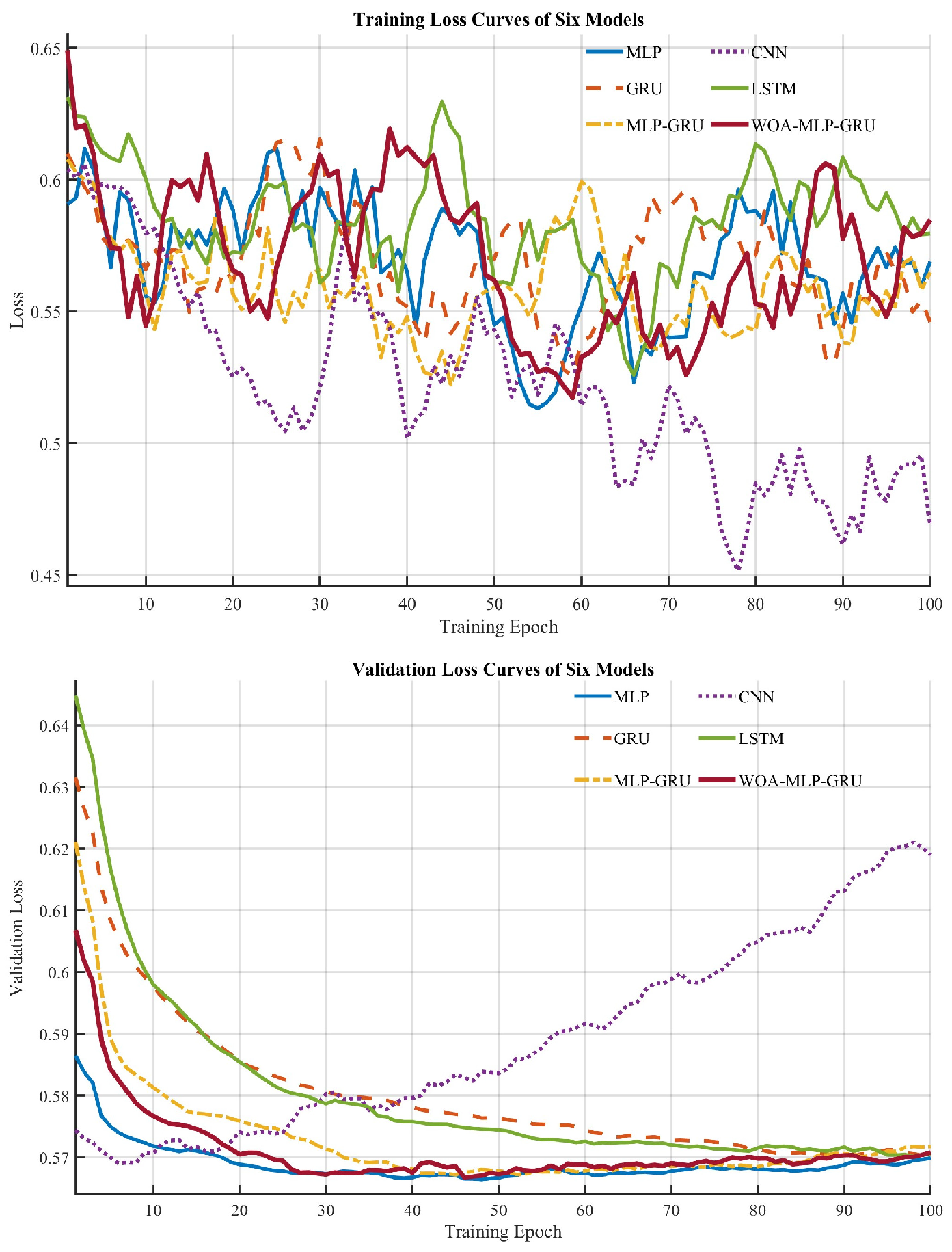
The final performance of a model depends not only on the network architecture itself, but also closely on the parameter updating behavior during training. Therefore, on the basis of the comparison of evaluation metrics, the number of training epochs was further uniformly set to 100, and the convergence characteristics and stability of different models were analyzed from the perspectives of training loss and validation loss.

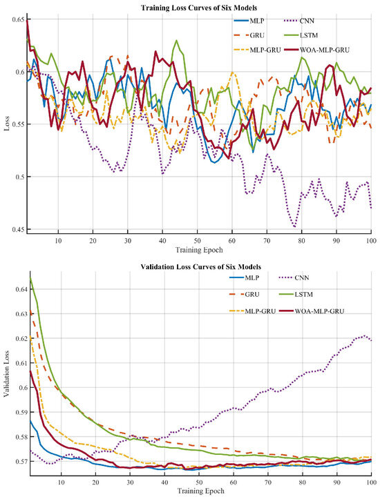
This section compares the convergence behavior and generalization capability of the six models. To ensure a fair comparison, all models were trained on the same dataset for 100 epochs. As shown in Figure 15, the training losses of all models decrease rapidly during the initial stage, indicating that each model is able to capture useful information from the input features. As training proceeds, however, clear differences gradually emerge. The single-structure models exhibit larger fluctuations in training loss, whereas the hybrid models show a comparatively more stable optimization process. Although CNN achieves a relatively low training loss in the later epochs, its validation loss begins to increase noticeably after approximately 40–50 epochs, revealing an increasing discrepancy between training and validation performance and therefore a stronger tendency toward overfitting.

Figure 15. Training loss and validation loss curves.

In contrast, the validation losses of MLP-GRU and WOA-MLP-GRU decrease rapidly and remain at relatively low levels during the middle and late stages of training. In particular, the WOA-optimized hybrid model maintains a smaller gap between training and validation losses, indicating that the optimized parameter configuration achieves a better balance between model fitting and generalization. Therefore, the loss curves provide process-level evidence that the MLP-GRU hybrid architecture improves training stability, while WOA-based hyperparameter optimization further enhances the generalization reliability of the proposed model.

5.4. Visual Analysis of Feature Separability

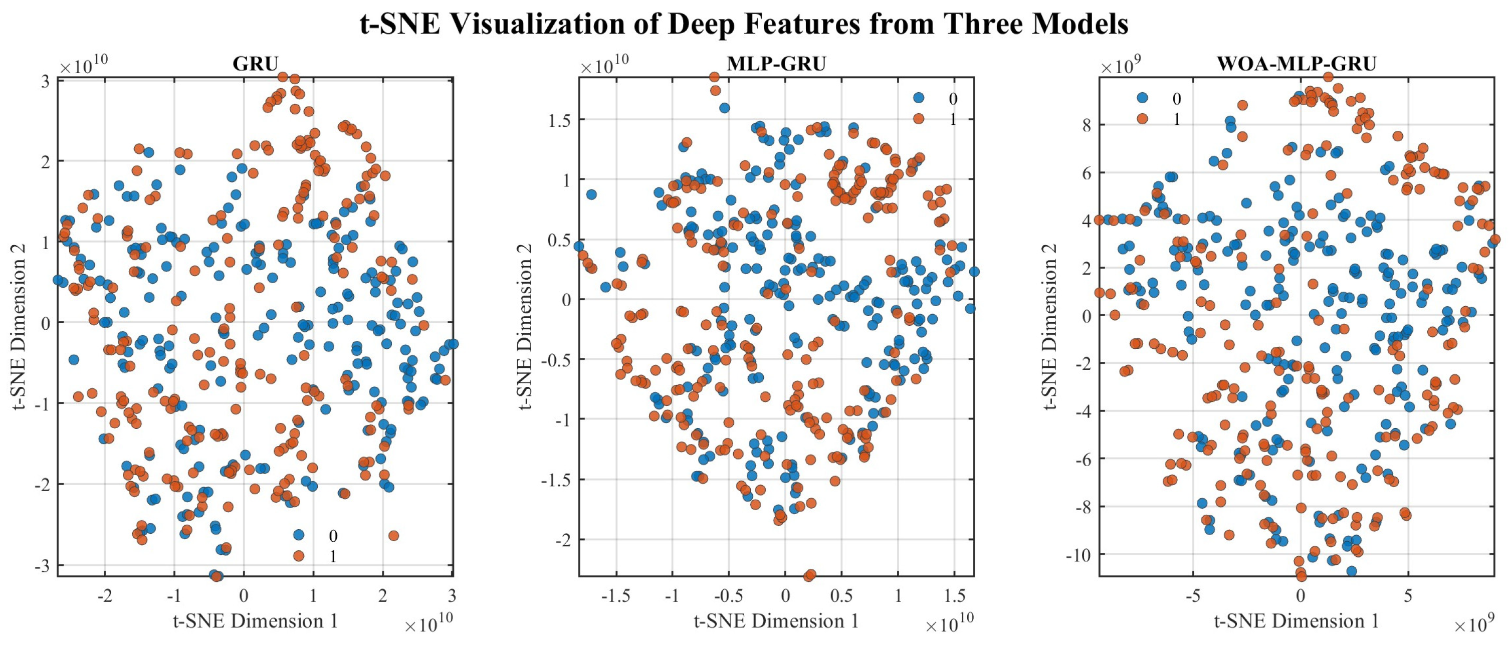
Section 5.2 and Section 5.3 have quantitatively evaluated the performance differences among models through evaluation metrics and convergence analysis. The results indicate that the MLP-GRU architecture improves classification performance and that WOA optimization further enhances the model performance under the current experimental settings. However, these quantitative results do not directly reveal how different models represent deep features. Therefore, t-SNE visualization is employed as a supplementary qualitative analysis to investigate the distribution characteristics of learned features.

The purpose of this section is not to perform another repetitive visualization comparison for all models, but to examine feature representation from the perspectives of the hybrid architecture design and the WOA-based hyperparameter optimization strategy. Therefore, only three representative models are selected. Specifically, GRU is taken as the baseline temporal model, MLP-GRU is used to evaluate the contribution of the hybrid architecture, and WOA-MLP-GRU is further employed to verify the effect of hyperparameter optimization while retaining the same backbone structure. Through this progressive comparison, the individual contributions of the hybrid design and the optimization strategy to feature representation can be more clearly revealed, while avoiding the loss of analytical focus caused by simultaneously presenting too many models.

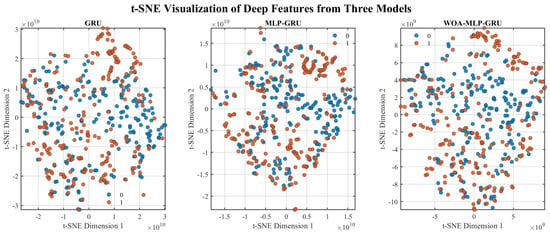
The cumulative explained variance of PCA for the three models exceeds 99%, indicating that the extracted deep features retain most of the information from the original feature space. The best t-SNE loss values of GRU, MLP-GRU, and WOA-MLP-GRU are 2.386, 2.404, and 2.373, respectively. Since t-SNE is a stochastic visualization method, the small differences in loss values are only considered as supplementary observations rather than quantitative evidence of model superiority. As shown in Figure 16, the GRU model exhibits considerable overlap between the two classes, suggesting that temporal features alone may not sufficiently capture the nonlinear characteristics of filter clogging. The MLP-GRU model achieves a more organized feature distribution by integrating nonlinear feature extraction with temporal modeling. The WOA-MLP-GRU model shows a relatively clearer class distribution, which may benefit from optimized hyperparameter selection. Nevertheless, the effectiveness of the proposed method is mainly supported by quantitative metrics and convergence analysis, while t-SNE provides only qualitative insight into feature representation.

Figure 16. t-SNE feature separability plot.

5.5. WOA Optimization Strategy Ablation Analysis

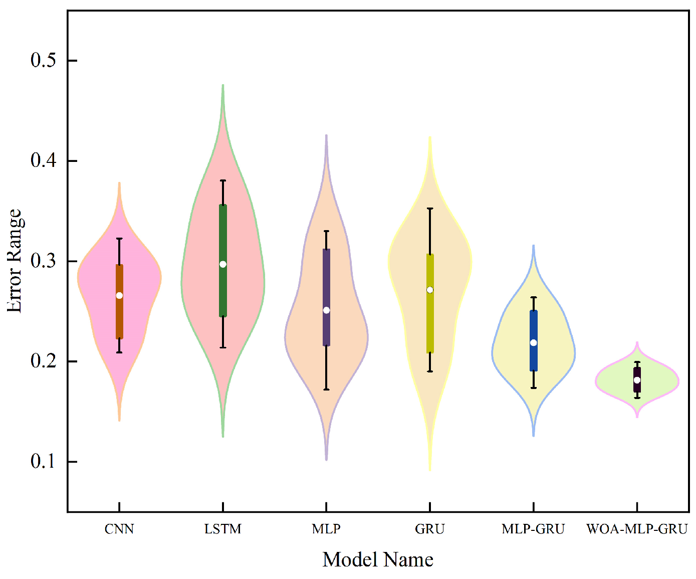
By comparing the error distributions of different models, this section further investigates, from the perspective of repeated experiments, whether WOA can effectively reduce model errors and improve the stability and robustness of model outputs.

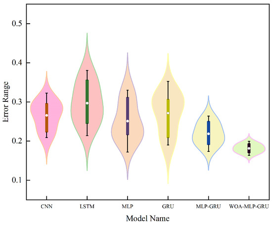
Figure 17 presents the violin distributions of the errors of the six models under repeated experimental conditions. It can be observed that the single models, including CNN, LSTM, MLP, and GRU, generally exhibit relatively high errors with wider distribution ranges, indicating larger error fluctuations and limited stability. By contrast, the error distribution of MLP-GRU shifts downward noticeably, suggesting that the hybrid architecture can effectively reduce identification errors and improve the model’s classification capability for fault samples. Furthermore, the WOA-MLP-GRU model achieves the lowest error distribution among all models, and its violin shape is more compact, indicating that after the introduction of the optimization strategy, the model not only attains a lower average error but also demonstrates better stability and robustness across repeated experiments.

Figure 17. Model Error Plot.

From the three progressive levels of validation, namely single-network models, hybrid models, and optimized models, the experimental results consistently show that the proposed WOA-MLP-GRU exhibits the best comprehensive performance in the task of return oil filter clogging fault identification. The underlying reason is that return oil filter clogging is not caused by an instantaneous abnormal event, but rather by the gradual accumulation of contaminants, which subsequently induces coupled variations in multiple variables such as pressure, flow, and temperature. This process is characterized by strong coupling, progressive evolution, and temporal dependency. A single network is generally insufficient to simultaneously capture the complex nonlinear relationships among multi-source features and the temporal dependencies involved in fault evolution. In contrast, the MLP-GRU model combines the nonlinear feature mapping capability of the MLP with the temporal modeling capability of the GRU, thereby enabling more effective extraction of discriminative information related to clogging faults and achieving joint representation of the coupling relationships and dynamic variation patterns of multi-source hydraulic features. On this basis, the WOA-based optimization strategy performs adaptive tuning of key hyperparameters, allowing a more reasonable balance to be achieved among model complexity, feature representation capability, and generalization performance. As a result, the model’s ability to capture intrinsic fault characteristics and its training stability are further enhanced.

6. Conclusions

This study proposes a mechanism-guided WOA-MLP-GRU framework for return-oil-filter clogging identification in excavator hydraulic systems. The main contribution is the integration of clogging-evolution mechanisms with multi-source operating variables, allowing the model to jointly characterize nonlinear feature interactions and temporal fault development. WOA is further used to optimize key network hyperparameters, while VMD analysis provides supplementary support for the pressure-evolution characteristics.

Experimental results based on real operating data demonstrate that the proposed method provides the best overall diagnostic performance among the compared models, achieving an Accuracy of 98.3%. Further evaluations of training convergence, feature separability, error distribution, and hyperparameter optimization confirm the effectiveness of the proposed framework. In particular, the combination of multi-source variables and temporal information reduces the possibility of confusing transient pressure increases caused by cold starts or operating-condition variations with progressive filter clogging. These findings indicate that the proposed method can provide a more reliable basis for return-oil-filter condition monitoring than conventional experience- or threshold-based diagnosis.

From an engineering perspective, the proposed method utilizes existing onboard pressure, temperature, and operating-state signals, which provides potential feasibility for integration into excavator controllers or cloud-based monitoring platforms without requiring additional dedicated sensing devices. However, the current study mainly focuses on offline clogging identification performance, and further investigations are still required regarding long-term online deployment, false alarm characteristics, maintenance effectiveness, and economic benefits in practical applications. Future work will extend the framework to more excavator models, operating conditions, and different fault severity levels, while incorporating remaining useful life prediction and field validation to further promote the transition from fault identification toward predictive maintenance.

References

- Feng, H.; Zhou, H.; Cao, D.; Yin, C.; Zhou, C. Data-driven hydraulic pressure prediction for typical excavators using a new deep learning SCSSA-LSTM method. Expert Syst. Appl. 2025, 275, 127078. [Google Scholar] [CrossRef] [Scilit]
- Luo, X.; Zhang, K.; Dong, S.; Wang, S.; Chen, H. Development and application of a multi-scale Thermal-Hydraulic coupling program for whole-core flow blockage analysis. Ann. Nucl. Energy 2025, 213, 111110. [Google Scholar] [CrossRef] [Scilit]
- Ding, R.; Cheng, M.; Jiang, L.; Hu, G. Active fault-tolerant control for electro-hydraulic systems with an independent metering valve against valve faults. IEEE Trans. Ind. Electron. 2020, 68, 7221–7232. [Google Scholar] [CrossRef] [Scilit]
- Soh, J.; Lee, C.; Kim, W.; Kang, B.; Kim, D. Anomaly Detection and Fault Diagnosis Based on Action States for Excavators. Appl. Sci. 2026, 16, 2414. [Google Scholar] [CrossRef] [Scilit]
- Chen, Q.; Wang, J.; Ahmed, Q. Design and evaluation of a structural analysis-based fault detection and identification scheme for a hydraulic torque converter. Sensors 2018, 18, 4103. [Google Scholar] [CrossRef] [Scilit] [PubMed]
- Kong, X.; Cai, B.; Yu, Y.; Yang, J.; Wang, B.; Liu, Z.; Shao, X.; Yang, C. Intelligent diagnosis method for early faults of electric-hydraulic control system based on residual analysis. Reliab. Eng. Syst. Saf. 2025, 261, 111142. [Google Scholar] [CrossRef] [Scilit]
- Zhu, Y.; Tang, S.; Yuan, S. Multiple-signal defect identification of hydraulic pump using an adaptive normalized model and S transform. Eng. Appl. Artif. Intell. 2023, 124, 106548. [Google Scholar] [CrossRef] [Scilit]
- Ng, F.; Harding, J.A.; Glass, J. Improving hydraulic excavator performance through in line hydraulic oil contamination monitoring. Mech. Syst. Signal Process. 2017, 83, 176–193. [Google Scholar] [CrossRef] [Scilit]
- Jeon, H.-G.; Kim, J.-K.; Na, S.-J.; Kim, M.-S.; Hong, S.-H. Application of condition monitoring for hydraulic oil using tuning fork sensor: A study case on hydraulic system of earth moving machinery. Materials 2022, 15, 7657. [Google Scholar] [CrossRef] [Scilit] [PubMed]
- Eker, O.F.; Camci, F.; Jennions, I.K. Physics-based prognostic modelling of filter clogging phenomena. Mech. Syst. Signal Process. 2016, 75, 395–412. [Google Scholar] [CrossRef] [Scilit]
- Wu, W.; Wang, S.; Chen, R.; Zhang, C.; Wang, Y.; Zhang, Y. Physics-informed recurrent neural network with cross-condition transfer for hydraulic oil filter degradation prognostics. Measurement 2026, 274, 121198. [Google Scholar] [CrossRef] [Scilit]
- Gao, H.; Huo, X.; Hu, R.; He, C. Optimized DTW-Resnet for fault diagnosis by data augmentation toward unequal length time series. IEEE Trans. Instrum. Meas. 2023, 72, 3532611. [Google Scholar] [CrossRef] [Scilit]
- Chennana, A.; Megherbi, A.C.; Bessous, N.; Sbaa, S.; Teta, A.; Belabbaci, E.O.; Rabehi, A.; Guermoui, M.; Agajie, T.F. Vibration signal analysis for rolling bearings faults diagnosis based on deep-shallow features fusion. Sci. Rep. 2025, 15, 9270. [Google Scholar] [CrossRef] [Scilit] [PubMed]
- Tang, S.; Khoo, B.C.; Zhu, Y.; Lim, K.M.; Yuan, S. A light deep adaptive framework toward fault diagnosis of a hydraulic piston pump. Appl. Acoust. 2024, 217, 109807. [Google Scholar] [CrossRef] [Scilit]
- Zhang, Z.; Wan, C.; Li, L.; Pang, Y.; Xiong, G.; Zhang, C.; Fan, X.; Wang, Y. CNN-IPINN: A method study on applying physics-informed neural networks to gear fault diagnosis. Meas. Sci. Technol. 2025, 36, 106101. [Google Scholar] [CrossRef] [Scilit]
- Sinitsin, V.; Ibryaeva, O.; Sakovskaya, V.; Eremeeva, V. Intelligent bearing fault diagnosis method combining mixed input and hybrid CNN-MLP model. Mech. Syst. Signal Process. 2022, 180, 109454. [Google Scholar] [CrossRef] [Scilit]
- Altobi, M.A.S.; Bevan, G.; Wallace, P.; Harrison, D.; Ramachandran, K. Fault diagnosis of a centrifugal pump using MLP-GABP and SVM with CWT. Eng. Sci. Technol. Int. J. 2019, 22, 854–861. [Google Scholar] [CrossRef] [Scilit]
- Hu, H.; Lu, H.; Shi, R.; Fan, X.; Deng, Z. A novel fault diagnosis method for key transmission sections based on Nadam-optimized GRU neural network. Electr. Power Syst. Res. 2024, 233, 110522. [Google Scholar] [CrossRef] [Scilit]
- Liu, B.; Fu, Z.; Hua, Z.; Zhang, J. Collision detection and fault diagnosis with DMAO-GRU for flow regulating valve. Meas. Sci. Technol. 2025, 36, 016238. [Google Scholar] [CrossRef] [Scilit]
- Wang, S.; Wang, C.; Lian, Y.; Luo, B. Research on Bearing Fault Diagnosis Based on VMD-RCMWPE Feature Extraction and WOA-SVM-Optimized Multidataset Fusion. Sensors 2025, 25, 5139. [Google Scholar] [CrossRef] [Scilit] [PubMed]
- Ding, C.; Yu, D.; Liu, X.; Sun, Q.; Zhu, Q.; Shi, Y. Research on Transformer Fault Diagnosis by WOA-SVM Based on Feature Selection and Data Balancing. IEEJ Trans. Electr. Electron. Eng. 2025, 20, 41–49. [Google Scholar] [CrossRef] [Scilit]
- Ma, W.; Ma, S.; Qiao, W.; Cao, D.; Yin, C. Research on PID controller of excavator electro-hydraulic system based on improved differential evolution. Machines 2023, 11, 143. [Google Scholar] [CrossRef] [Scilit]
- Feng, H.; Jiang, J.; Chang, X.; Yin, C.; Cao, D.; Yu, H.; Li, C.; Xie, J. Adaptive sliding mode controller based on fuzzy rules for a typical excavator electro-hydraulic position control system. Eng. Appl. Artif. Intell. 2023, 126, 107008. [Google Scholar] [CrossRef] [Scilit]
- Stosiak, M.; Karpenko, M.; Skačkauskas, P. Variations in the pressure pulsation spectrum of a hydraulic system with an oscillating relief valve. Adv. Mech. Eng. 2025, 17, 16878132251343945. [Google Scholar] [CrossRef] [Scilit]
- Stosiak, M.; Karpenko, M.; Deptuła, A.; Urbanowicz, K.; Skačkauskas, P.; Cieślicki, R.; Deptuła, A.M. Modelling and Experimental verification of the interaction in a hydraulic directional control valve spool pair. Appl. Sci. 2022, 13, 458. [Google Scholar] [CrossRef] [Scilit]
- Karpenko, M.; Prentkovskis, O.; Šukevičius, Š. Research on high-pressure hose with repairing fitting and influence on energy parameter of the hydraulic drive. Eksploat. Niezawodn. 2022, 24, 25–32. [Google Scholar] [CrossRef] [Scilit]
- Karpenko, M.; Bogdevičius, M. Investigation of Hydrodynamic Processes in the System–“Pipeline-Fittings”. In Proceedings of the International Conference TRANSBALTICA: Transportation Science and Technology; Springer International Publishing: Cham, Switzerland, 2019; pp. 331–340. [Google Scholar] [CrossRef] [Scilit]
- Yu, F.; Ran, M.; Xiang, W.; Xiong, J.; Bai, Y. Short-term load forecasting of integrated energy system based on improved complete ensemble empirical mode decomposition with adaptive noise maximum information coefficient transformer. Energy Explor. Exploit. 2025, 44, 685–712. [Google Scholar] [CrossRef] [Scilit]
- Elsayed, W.M.; Alsabaan, M.; Ibrahem, M.I.; El-Shafeiy, E. The potential of deep learning in underwater wireless sensor networks and noise canceling for the effective monitoring of aquatic life. Sensors 2024, 24, 6102. [Google Scholar] [CrossRef] [Scilit] [PubMed]
- Cui, X.; Zhu, J.; Jia, L.; Wang, J.; Wu, Y. A novel heat load prediction model of district heating system based on hybrid whale optimization algorithm (WOA) and CNN-LSTM with attention mechanism. Energy 2024, 312, 133536. [Google Scholar] [CrossRef] [Scilit]
- Zhang, J.; Li, S.; Liu, X.; Chen, H.; Zhou, Q. A WOA-ICEEMDAN joint wavelet threshold function based denoising method for ultrasound signals. Nondestruct. Test. Eval. 2026, 41, 278–313. [Google Scholar] [CrossRef] [Scilit]
- Wang, Y.; Tao, J.; Zhao, L. Incremental multi-step learning MLP model for online soft sensor modeling. Sensors 2025, 25, 4303. [Google Scholar] [CrossRef] [Scilit] [PubMed]
- Das, T.; Guchhait, S. A hybrid GRU and LSTM-based deep learning approach for multiclass structural damage identification using dynamic acceleration data. Eng. Fail. Anal. 2025, 170, 109259. [Google Scholar] [CrossRef] [Scilit]
- Miao, Y.; Xia, Y.; Liu, J. Remaining useful life prediction via a double convolutional attention-based CNN-GRU model. IEEE Trans. Instrum. Meas. 2025, 74, 3544313. [Google Scholar] [CrossRef] [Scilit]
Disclaimer/Publisher’s Note: The statements, opinions and data contained in all publications are solely those of the individual author(s) and contributor(s) and not of MDPI and/or the editor(s). MDPI and/or the editor(s) disclaim responsibility for any injury to people or property resulting from any ideas, methods, instructions or products referred to in the content. |
© 2026 by the authors. Licensee MDPI, Basel, Switzerland. This article is an open access article distributed under the terms and conditions of the Creative Commons Attribution (CC BY) license.