


Abstract
Wind turbine bearings operate long-term under complex and variable operating conditions, where fault impulse characteristics are easily submerged by strong noise. Traditional graph signal processing-based bearing fault diagnosis methods are limited by fixed graph topology, empirical feature selection and poor noise robustness. This paper proposes an adaptive frequency graph spectrum (AFGS) model for bearing fault diagnosis. The model constructs graph signals in the frequency domain and determines the core analysis interval adaptively via eigenvalue sequences, which eliminates fixed topology constraints. Combined with a fast bisection search framework and a correlation spectral negative entropy (CSNE) index sensitive to periodic fault impulses, the proposed method realizes fully automatic optimal band selection without manual intervention and improves noise resistance. The AFGS method first transforms vibration signals via fast Fourier transform and constructs frequency-domain graph features based on Laplacian matrix decomposition. The optimal fault characteristic band is adaptively determined using the bisection framework and CSNE criterion. Finally, signal reconstruction and envelope spectrum analysis are implemented for fault identification. Simulation results under −3 dB low signal-to-noise ratio show that AFGS can effectively extract the 1st to 8th fault harmonics. Further validation on the measured inner and outer race fault signals of 6205 bearings demonstrates that the proposed method can clearly identify fault characteristic frequencies and their multi-order harmonics. Comparative tests with Fast Kurtogram and Autogram indicate that the two benchmark algorithms only extract limited low-order harmonics under simulated noise and completely fail in practical strong noise environments. Experimental results verify that AFGS outperforms conventional methods in band localization accuracy, noise suppression, and fault feature extraction completeness, providing a reliable solution for the bearing fault diagnosis of rotating machinery under complex working conditions.
1. Introduction
As a core topic in the field of wind turbine health management, bearing fault diagnosis has attracted significant research attention from the academic community, with in-depth explorations conducted in three major areas: noise-robust signal processing, effective fault feature extraction, and the performance optimization of diagnostic models, with graph signal processing and spectral analysis becoming core technological pillars [1].
In practical wind turbine condition monitoring systems, vibration acceleration sensors are the most mainstream sensing hardware for assessing bearing health. The sensor is installed on the surface of the bearing housing or gearbox housing to collect vibration acceleration signals. When a bearing experiences damage such as spalling or cracking, periodic impact components are excited in the vibration response. However, the vibration signals collected on-site are inevitably contaminated by strong background noise from gear meshing, airflow, and mechanical transmission, and are also accompanied by time-varying disturbances in load and rotational speed, posing a significant challenge to fault feature extraction.
To address challenges in wind turbine bearing diagnosis—such as high noise levels, varying operating conditions, limited sample sizes, and operating condition shifts—researchers have successively proposed various improved methods: a sparse framework integrating frequency-slicing functions can enhance weak fault features [2]; high-dimensional optimization-based chirp transform extraction is suitable for analyzing complex non-stationary signals; self-supervised learning in both time and frequency domains effectively improves diagnostic performance with limited samples; and the combination of wavelet principal component analysis with a cross-domain attention network enhances the algorithm’s generalization capability across different operating conditions [3,4]. However, wind turbines operate under complex conditions, facing problems such as strong noise interference, load fluctuations, and frequent changes in speed. Existing methods still have significant limitations, and more robust and adaptive diagnostic technologies need to be developed. Various algorithms have been developed to address specific diagnostic challenges: A spherical tree-structured phase-space warping algorithm enables the precise tracking of bearing degradation under variable speeds [5]; a multivariate cyclization deep deconvolution algorithm enhances fault identification performance amidst strong interference [6]; an iterative correction-based variational mode extraction method effectively isolates transient fault features in noisy environments [7]; and a clustering low-rank tensor-train dynamic mode decomposition algorithm is suitable for the fault analysis of multivariate signals [8].
Early research on graph signal processing laid the theoretical foundation for the analysis of non-stationary signals. To address the scarcity of fault samples for wind turbine drivetrain equipment, a convex optimization-based differential analysis model achieves unsupervised fault diagnosis within a spectrum framework, demonstrating excellent generalization capabilities [9]; meanwhile, a differential strategy combining amplitude modulation with variational filtering enables the precise extraction of bearing fault features in environments with strong interference [10]. Shi and Moura [11] extended discrete signal processing to irregular graph structures, defined vertex domain and spectral domain shift operators, and implemented convolution and modulation operations based on the graph Fourier transform (GFT), providing a framework for processing complex correlation features in the vibration signals of wind turbine bearings. Hammond et al. [12] constructed a graph wavelet framework (SGWT) based on the spectral decomposition of the graph Laplacian matrix and achieved fast calculation through Chebyshev polynomial approximation. The localization characteristics of this framework provided theoretical support for capturing fault impact signals and promoted the initial application of graph theory in mechanical fault diagnosis. An et al. [13] applied the inherent time scale decomposition (ITD) method to the fault diagnosis of wind turbine bearings. By extracting the frequency center of the appropriate rotation component as the feature vector and combining it with the nearest neighbor algorithm to achieve fault identification, the feasibility of graph spectral theory in the fault diagnosis of wind turbine bearings was verified. With the deepening of application-oriented research, scholars have continuously optimized graph-based diagnostic strategies. Ou and Yu mapped the rolling bearing vibration signal to a road map, extracted the Laplace energy as a fault feature, and combined it with Mahalanobis distance (MD) to complete the classification. A high-accuracy diagnosis was achieved with a small number of samples. However, this method relied only on a single graph domain feature and failed to solve the dynamic matching problem between the fixed graph topology and the time-varying fault features of wind turbine bearings [14]. Furutani et al. proposed a graph signal processing framework for directed graphs based on the Hermitian Laplace matrix. By encoding the direction information of the edges into complex phases, they realized the spectral analysis of directed graphs while maintaining the Hermitian property, providing a new idea for processing the directional correlation features in the vibration signal of wind turbine bearings [15]. Ruiz et al. [16] systematically established the limit theory of graph signal processing—the graph neural signal processing framework (WSP)—and proved the convergence of graph Fourier transform and graph filters to this framework under convergent graph sequences, providing a mathematical basis for the signal analysis of large-scale dynamic wind power networks.
In the field of time–frequency domain fusion and composite fault diagnosis, researchers have also carried out substantial work. Tang et al. proposed a deep feature fusion method based on complete ensemble empirical mode decomposition and the second fast Fourier transform. The method combines chi-square test and recursive feature elimination to screen optimal features. A high recognition rate has been verified on measured data. However, the feature dimension of this method is prone to expansion and its sensitivity to early weak faults is insufficient [17]. In a separate study, Dhamande and Chaudhari [18] presented a statistical feature extraction technique specifically designed for composite gear-bearing faults. The core of their method relies on combining continuous wavelet transform (CWT) and discrete wavelet transform (DWT) to capture fault-related information. By extracting statistical quantities such as standard deviation and variance from different decomposition scales, this method effectively improves the recognition accuracy of composite faults. However, this method relies heavily on manually designed features and exhibits weak generalization ability under varying working conditions. In another study, Dhamande and Chaudhari presented a statistical feature extraction technique specifically designed for composite gear-bearing faults. The core of their method relies on combining continuous wavelet transform (CWT) and discrete wavelet transform (DWT) to capture fault-related information. The method achieves layer-by-layer screening of features through the chi-square test, variance-Relief-F, and hierarchical clustering, which effectively reduces feature redundancy. However, the feature stability under strong noise environments still needs to be further improved [19].
Scholars have also made active explorations in the areas of noise interference resistance and weak fault extraction. The adaptive minimum entropy deconvolution method proposed by Sun and Yu based on sparse representation and adjacent signal difference effectively enhances the fault pulse characteristics by embedding the adaptive sparse representation into the iterative calculation of minimum entropy deconvolution. However, this method is sensitive to the length of the inverse filter and does not make full use of the advantages of graph theory in multi-scale feature representation [20]. To improve spectrum sensing performance, Hu and co-workers designed a novel algorithm based on the graph Fourier transform. Corresponding detection statistics can be established by combining the Laplacian matrix with the vertex probability vector. Good detection performance was shown under low signal-to-noise ratio conditions. However, this method is mainly aimed at spectrum sensing tasks in cognitive radio. Its applicability in rotating machinery fault diagnosis still needs further verification [21]. Usta and Akay defined graph cepstrum as a new tool for homomorphic processing of graph signals. By combining the graph Fourier transform with logarithmic operation, they realized the separation of convolution quantities in the graph domain, providing a new analytical means for decoupling fault pulses and transmission paths in wind turbines bearing vibration signals [22].
In terms of the systematic fault analysis of wind turbine bearings, Liu and Zhang [23] systematically reviewed the fault modes and condition monitoring methods of large wind turbine bearings, pointing out that wind turbine bearings have diverse fault types and that the fault characteristics of different components such as main bearings, gearbox bearings, generator bearings, and pitch bearings are significantly different. An urgent need exists to develop intelligent diagnostic methods that are highly adaptable, have good noise resistance, and require no manual intervention. Wei and Yu [24] proposed the Hermitian random walk graph Fourier transform for directed graphs. By constructing the Hermitian random walk Laplace operator, they obtained an orthogonal Fourier basis while maintaining the direction information, providing a theoretical tool for dealing with the asymmetric transmission path problem in the vibration signals of wind turbine bearings.
Existing diagnostic methods suffer from the following problems: fixed graph topology cannot adapt to time-varying faults, poor immunity to strong noise, low identification of early and weak faults, weak generalization ability of manually designed features, serious feature redundancy, insufficient multi-scale graph feature mining, and difficulty in adapting to the differentiated faults of multiple components in wind turbine bearings. To address these issues, an adaptive fault feature localization method for wind turbine bearings based on adaptive frequency graph spectrum model (AFGS-Model) is proposed in this paper. First, a Laplacian moment eigenvalue decomposition method based on Fourier spectrum amplitude is constructed, successfully avoiding noise interference in the graph construction process. After determining key points based on the eigenvalue sequence, the optimal fault feature order band is adaptively searched using a fast bisection framework. The correlation spectral negentropy (CSNE), which is sensitive to fault features, is used to evaluate the information in the order band to achieve frequency band selection without manual intervention. Simulation and experimental results demonstrate that this method has excellent fault identification capability and robustness in strong noise environments.
It should be noted that the AFGS Model proposed in this paper is currently mainly validated for approximately stationary operating conditions with relatively stable rotational speeds. While the fast Fourier transform (FFT) is suitable for stationary signal analysis, real wind turbines operate under non-stationary conditions with varying rotational speeds. The actual rotational speed of the turbine’s main shaft can be as low as a few revolutions per minute, resulting in an extremely low fundamental frequency. It is worth noting that although the turbine’s main shaft frequency is very low, the fault characteristic frequencies generated by the impact of the bearing rolling elements are amplified by the bearing’s geometric parameters, placing the fault impact components in the mid-to-high frequency range. Therefore, vibration sensors can still collect fault information that can be used for diagnosis. Nevertheless, the highly non-stationary operating conditions with large-range rotational speed fluctuations and the extremely low rotational speed of the main shaft remain significant limitations of this method at this stage [25]. For such conditions, it is necessary to combine preprocessing techniques such as order tracking and angle resampling to convert the non-stationary time-domain signal into a stationary signal in the order domain. This will be a key research direction in the future.
The rest of this paper is organized as follows. Section 2 introduces the fundamental theory of graph signal processing. Section 3 elaborates the principle and implementation workflow of the AFGS Model. Section 4 carries out simulation verification and a comparative study with Fast Kurtogram and Autogram [26,27]. Section 5 validates the proposed method using measured bearing fault signals. Section 6 presents the conclusions.
2. Theoretical Background
Graph signal processing contains a wealth of fundamental concepts. To help readers understand the mathematical origins of the AFGS Model in this paper, this section first introduces the general fundamental definitions of graph signal processing; subsequently, the specific application of each part of the fundamental theory in the adaptive frequency spectrum (AFGS) model in this paper is clarified.
In the field of graph signal processing, time-domain signals are commonly mapped onto graph structures to facilitate analytical research. With the development of this field, the representation of graphs has become increasingly diverse. A graph can be defined as an ordered binary pair consisting of a vertex set and an edge set. Vertices correspond to individual data points, while edges serve to link any two vertices, representing the relationships between the data points. If the two vertices connected by an edge are unordered, such an edge is defined as an undirected edge; otherwise, it falls into the category of directed edges, namely a directed edge. As shown in Figure 1, if two vertices have similar amplitudes, a connection exists between them.
Figure 1.
Time series and its horizontal visibility graph.
Figure 2a,b shows the nearest neighbor graphs, which are constructed according to the nearest neighbor rule. If two points are sufficiently close, a connection is established, and the two graphs represent a directed graph and an undirected graph, respectively.
Figure 2.
Directed and undirected graphs.
Figure 3a shows the simplest roadmap structure, where only adjacent vertices are connected. This structure is often used in time-series data such as vibration signals and electrocardiogram signals. When any two vertices are connected by an edge, a complete graph is formed, as shown in Figure 3b.
Figure 3.
Road graph and complete graph.
The above-mentioned horizontally visible graphs, k-nearest neighbor graphs, path graphs, and complete graphs are typical topological forms in the field of graph signal processing. Although this paper does not directly adopt the above topologies, it introduces them to illustrate the basic modeling ideas of graph signals. The AFGS Model in this paper is based on the dynamic construction of weighted undirected graphs from frequency-domain amplitude sequences.
To represent graph signals, degree matrices, adjacency matrices, and Laplacian matrices are typically used. The elements in the adjacency matrix represent the connections between nodes. In undirected graphs, this matrix is symmetric, and the value indicate whether an edge exists between nodes i and j (1 for existence, 0 for absence). In directed graphs, the matrix is usually asymmetric, representing an edge where node i points only to node j. In weighted graphs, the elements represent the weights between nodes; the weighting method can be determined based on the signal characteristics of the specific problem, thus selecting appropriate weights.
Both the constant weight assignment of 1 and the weighting scheme based on the heat kernel function fail to account for the inherent differences between certain nodes. To improve the performance of the model, the Euclidean distance is adopted as the weighting strategy, as formulated in Equation (1). This weighting method can take into account both the relationship between connecting edges and the differences between vertices. The degree matrix is a diagonal matrix, and its function is to reflect the inherent attributes of each node. As shown in Equation (2), the element corresponding to each row in this matrix is numerically equivalent to the sum of all elements in the corresponding row of the adjacency matrix, and each element in the matrix can also be used to characterize the importance of the corresponding node.
The role of the adjacency matrix and degree matrix in the AFGS Model. The adjacency matrix and degree matrix are the prerequisites for constructing the Laplace matrix from the frequency-domain amplitude sequence in Section 3.1; this paper adopts the Euclidean distance weighting strategy to construct the graph adjacency weights corresponding to the frequency-domain signal.
The Laplacian matrix has significant applicability and effectiveness in graph signal processing tasks. As shown in Equation (3), this matrix incorporates the relevant parameters of the adjacency matrix and the degree matrix, which endows the Laplacian matrix with the inherent properties of the two types of matrices above-mentioned, enabling it to more comprehensively and accurately characterize the overall structural features of the graph.
To obtain the important information contained in the Laplacian matrix, the matrix needs to undergo eigenvalue decomposition, which can be expressed as:
In this context, p is the order variable, ranging over the set p = 1, 2…, n. The parameter in turn corresponds to the total number of vertices contained in the constructed graph. After conducting eigenvalue decomposition on the graph Laplacian matrix, the matrix composed of each eigenvector is denoted as , and the corresponding eigenvalue matrix can be represented as
3. Adaptive Frequency Graph Spectrum Model
In signal transformation, the Fourier transform is theoretically a reversible transform, and the original time-domain signal can be reconstructed without information loss by completely preserving the amplitude and phase. This method completely preserves the spectral phase information during the transformation from the time domain to the frequency domain, and only uses the amplitude sequence to construct the graph signal; the original phase is reused in the signal reconstruction stage, thereby avoiding the risk of loss of effective information caused by the frequency domain transformation.
As noise levels rise, periodic fault components in time-domain signals are often completely masked. Conventional approaches that convert time-domain signals directly into the frequency domain for diagnostic analysis often struggle to deliver reliable fault detection results, particularly under high noise conditions. To suppress the adverse effects of noise, an adaptive frequency graph spectrum model (AFGS Model) is proposed in this paper. This method overcomes the limitations of direct time-domain conversion by first converting the signal to the frequency domain and then further mapping it to a spectral representation. After obtaining the frequency-domain spectral bands, an adaptive strategy based on a bisection method is introduced to select the optimal order band, thereby achieving accurate bearing fault diagnosis. The overall process of this method is shown in Figure 4, and the specific implementation steps are as follows.
Figure 4.
Flowchart of the proposed method.
- (1)
- The collected time-domain vibration signal is processed by fast Fourier transform to convert it into the frequency domain, with the amplitude and phase information of the spectrum retained.
- (2)
- The amplitude sequence of the spectrum is used, and then the eigenvalue spectrum of the matrix is obtained through eigenvalue decomposition.
- (3)
- The graph structure is established based on the eigenvalue spectrum, and the graph Fourier transform is calculated to generate the graph frequency spectrum.
- (4)
- Based on the eigenvalue sequence, the spectrum feature map is then refined, and the last 128 nodes are selected as the key spectrum feature bands.
- (5)
- A fast bisection framework is constructed on the extracted key spectral feature bands, and the optimal order interval is searched.
- (6)
- The CSNE is used as the evaluation indicator to sequentially search for high-level sub-intervals and iteratively optimize the process.
- (7)
- The CSNE value is retained as the search range for the next round. This process is repeated until the preset convergence condition is met or the search interval reaches the minimum precision, and the finally determined order interval with the optimal indicator value is taken as the best order band.
- (8)
- With the reconstructed time-domain signal corresponding to the final optimal order band and its envelope spectrum obtained, the fault diagnosis procedure is concluded.
3.1. Frequency Domain Feature Graph Model
Graph theory, as a key analytical tool for graph-structured data, finds extensive use in areas such as machine learning, dimensionality reduction, and signal processing. This framework uncovers the inherent structural patterns within a graph by examining the spectral characteristics of its associated matrices.
In fault diagnosis, periodic impulses in time-domain signals are easily masked by noise, increasing the difficulty of feature extraction. Therefore, the graph Fourier transform is innovatively applied in this paper to frequency-domain signals, extracting features based on the distribution characteristics of faults in the frequency domain. Traditional methods use Fourier transform for frequency-domain conversion, but their global processing approach may limit the accuracy of the analysis. Therefore, this paper uses fast Fourier transform to achieve time–frequency conversion, as defined below:
In this context, g(n) represents the discrete vibration signal in the time domain, while G(f) is its corresponding spectral-domain form, which preserves both amplitude and phase characteristics. The variable N denotes the total number of samples in the discrete sequence.
The fast Fourier transform (FFT) allows for the conversion of signals from their original time-domain form into the frequency-domain representation, simultaneously acquiring both amplitude and phase information. To ensure information integrity, the phase information is retained in subsequent processing, and the graphical signal is primarily constructed based on the signal’s amplitude. The frequency-domain amplitude expression is shown below:
In some cases, fault characteristics are more pronounced in the frequency domain than in the time domain. To fully exploit the advantages of frequency-domain analysis, the approach proceeds as follows: first, a graph signal is built using the amplitude information extracted from the frequency domain. Then, by applying the graph Fourier transform to this constructed graph signal, the corresponding spectral representation of the original signal can be derived. The mathematical model and matrix representation of the frequency-domain spectrum are defined as follows:
Here, f(p) denotes the frequency-domain spectral sequence, and d is the corresponding eigenvector associated with this sequence. Selecting a suitable sub band from the frequency-domain spectrum and reconstructing the signal using inverse graph Fourier transform yields the following matrix representation:
Once the frequency-domain spectrum is acquired, it is analyzed to select several suitable orders for inverse graph Fourier transform, which produces updated amplitude information . To facilitate subsequent signal processing and analysis, the updated amplitude information must be paired with the original phase information, thereby forming a new composite frequency-domain signal . Subsequently, the signal is reconstructed by applying the inverse fast Fourier transform (IFFT), yielding a new time-domain sequence . The fault diagnosis process is then completed by computing the Hilbert envelope spectrum of the reconstructed signal. The mathematical formulation of the inverse fast Fourier transform is defined below:
Spectral clustering offers easy implementation and superior clustering performance, and is thus widely applied in practical scenarios. This work utilizes the inherent clustering characteristics of the Laplacian matrix to construct the basic functions for the graph Fourier transform. The transform decomposes the graph signal into a linear combination of eigenvectors of varying orders, thereby establishing a mapping between the vertex domain and the order dimension of the graph spectral domain, which enables the frequency-domain spectrum to contain rich structural information.
3.2. Binary Search Method for Optimal Fault Feature Order Band
To address the issues of traditional frequency band selection methods relying on manual experience and suffering from low computational efficiency, this paper proposes a fully adaptive frequency band partitioning strategy based on the bisection method. This method departs from fixed interval partitioning or sliding window traversal; its core innovation lies in its intelligent processing of the complete frequency-domain spectrum directly, without the need for empirical knowledge or manual intervention. Starting from the selected whole frequency band, the algorithm iteratively divides the original frequency band into increasingly finer sub-bands through bisection and selects an indicator as a quantitative evaluation criterion for comparison at each level.
The algorithm’s execution flow consists of three main stages: initialization, iterative search, and result output. Its purpose is to find the optimal interval that maximizes the evaluation value, with representing the interval. Observing the eigenvalue sequence as shown in Figure 5a, the larger the eigenvalue, the more important the eigenvalue vector, and this can be reflected in the frequency-domain spectrum, as shown in Figure 5b. Fault information is concentrated within a certain order range; therefore, it is not necessary to select all orders. This section only selected the last 128 nodes for the binary search.
Figure 5.
Eigenvalues and frequency-domain spectra.
The algorithm starts with the selected integer frequency-domain spectrum sequence . The initial search interval is set to the global frequency band.
Simultaneously, convergence condition parameters are preset. The most critical parameter is the minimum interval length threshold , which determines the final output accuracy of the algorithm. To ensure the accuracy of frequency band selection and improve frequency resolution, in this method is set to 4.
The hyperparameters involved in this paper mainly include the minimum interval length threshold for the binary search, and the selection of the last 128 nodes as the core analysis interval.
Minimum interval length : This parameter determines the termination condition of the binary iteration and controls the output order bandwidth. This value was not obtained through repeated trial and error: if the value is too large, the order bandwidth will be too wide and easily mixed with a lot of noise; if the value is too small, the interval will be too narrow, and the fault features will be segmented. Considering the overall spectrum order resolution and the order distribution corresponding to the fault impact, is set to ensure the frequency band resolution while avoiding the fault features being over-segmented.
The last 128 nodes were selected: Based on the distribution pattern of Laplace eigenvalues, the spectral components corresponding to high-order eigenvalues contain high-frequency details related to fault impact. Considering the eigenvalue sequence distribution characteristics under the sampling parameters used in this paper, the last 128 nodes were selected to balance computational complexity and fault feature capture capability. This parameter can be adaptively adjusted according to the number of sampling points; under the experimental conditions in this paper, it was fixed at 128.
The second step involves a recursive binary search. In each iteration , the current search interval is precisely divided into two sub-intervals. First, the midpoint of each sub-interval is calculated:
Generate two non-overlapping continuous sub-intervals based on the midpoint position:
This division method ensures that the orders of the two sub-intervals differ by no more than 1, thus guaranteeing the balance of the search.
The algorithm performs independent signal processing and quality assessment on two sub-intervals simultaneously. This process includes frequency-domain feature extraction, signal reconstruction and transformation, and quality indicator calculation. The processing of the two sub-paths is completely independent, which effectively improves the algorithm’s execution efficiency.
After obtaining the evaluation results for the two sub-intervals, the algorithm compares them and makes a decision. Let denote the frequency band quality evaluation function, then the decision rule is:
This decision-making mechanism ensures that the algorithm always searches in the direction of higher quality.
After each iteration, check whether the length of the current interval satisfies the convergence condition:
If the condition is met, the iteration terminates and enters the output stage; otherwise, let the condition be met and return to step 1 to continue the search. The specific operation is illustrated in Figure 6.
Figure 6.
Eigenvalues and frequency-domain spectra. Schematic diagram of determining the optimal fault frequency band using the bisection method.
When the iteration terminates, the current search interval is the optimal fault characteristic frequency band determined by the algorithm. Output the boundary information of this frequency band .
The binary search algorithm starts from the entire frequency band, requiring no prior knowledge about the fault frequency or band location. It is entirely data-driven, avoiding biases introduced by manually preset parameters. Furthermore, the binary search algorithm has a logarithmic complexity, a significant advantage over the linear complexity of the traditional sliding window method. This makes it particularly suitable for applications with high computational efficiency requirements, such as online monitoring and real-time diagnosis. Another key advantage of this strategy is its fully adaptive nature. Traditional methods often rely on expert experience to pre-set key parameters, such as the width and step size of the sliding window, or fixed frequency band boundaries. These parameter settings are not only highly subjective, but also require repeated adjustments under different operating conditions, severely limiting the method’s versatility and automation. The binary search algorithm completely eliminates this parameter dependence, requiring only a loose convergence threshold. The entire search process is entirely data-driven, automatically making decisions through the objective comparison of spectral values, eliminating uncertainties introduced by human intervention, and ensuring the consistency and repeatability of diagnostic results.
3.3. Correlation Spectral Negentropy
During the steady-state operation of rotating machinery, the collected vibration signals typically reflect the system’s balanced operating state. Nevertheless, once key components like bearings or gears develop faults, this equilibrium is disrupted when faults occur (e.g., inner or outer ring peeling of bearings, gear tooth breakage). The vibration signals not only generate pulses, but these pulses also exhibit significant periodicity. An inherent similarity and correlation exist between the pulses generated by a previous impact and those generated by subsequent impacts. Using correlation analysis to process the signal can effectively amplify the periodic characteristics it contains. Conversely, random noise and accidental impacts make it difficult to find similar components in the signal, exhibiting extremely poor autocorrelation. The impact information caused by a fault disrupts the original equilibrium state of the system; after correlation processing, the signal’s entropy will drop significantly. For this reason, like kurtosis, entropy is also an effective basis for detecting imbalanced disturbances in the system.
Given the signal as , its spectrum can be calculated using Fourier transform . Based on the minimum points of the trend spectrum, the signal spectrum is divided into frequency bands, with the boundaries of each band denoted as , where . The center frequency of each band is , and the bandwidth is . For each signal component within a frequency band, the squared envelope is calculated. Then, the unbiased autocorrelation function of this envelope signal is calculated as follows:
where is the time delay factor
It is worth noting that the unbiased autocorrelation function used in Equation (16) is theoretically more sensitive to the non-stationary characteristics of the signal, and the statistical properties of this operator assume wide stationary random signals.
In the complete AFGS algorithm flow presented in this paper, the autocorrelation operation is not directly applied to the original acquired vibration signal, but rather to the narrowband squared envelope component after bandpass filtering. After bandpass filtering, only the narrowband oscillation component corresponding to the bearing fault impact is retained within the target frequency band. This narrowband component approximately satisfies the wide stationarity condition under the approximately stationary operating conditions studied in this paper, thereby mitigating the autocorrelation calculation bias caused by the non-stationarity of the original signal.
To visually demonstrate the impact of variable speed non-stationary operating conditions on the autocorrelation calculation of Equation (16), two sets of comparative numerical simulations were conducted here. The simulations were uniformly set with a sampling frequency and a sampling point number .
Operating Condition 1 (Constant Speed—Approximately Stable): The bearing failure impact has a fixed period of and a fault characteristic frequency of . Damped oscillating pulses are used to simulate the bearing impact, superimposed with Gaussian white noise, and the impact times are strictly equal.
Operating Condition 2 (Variable Speed—Simulated Fan Non-Stability): The instantaneous frequency of the fault changes linearly with time , and the fault impact time interval continues to drift; the pulse damping parameters and noise intensity were completely consistent with those of Operating Condition 1 to ensure fair comparison.
Two sets of signals were filtered using identical bandpass filters to obtain narrowband outputs. The squared envelope was calculated and then substituted into Equation (16) to calculate the global unbiased autocorrelation. Simulation results show that under constant speed and stationary conditions, the autocorrelation function can form sharp peaks at the fault period and its double delay position, effectively characterizing the periodicity of the fault and contributing to a higher CSNE evaluation value. Under variable speed and non-stationary conditions, since Equation (16) uses global time averaging, the impact time of the drift cannot be aligned at the same delay position, the autocorrelation peak corresponding to the fault is significantly flattened, the peak amplitude is greatly attenuated, and the energy is spread out. This degradation directly reduces the concentration of the energy flow function, causing a decrease in the CSNE index. Even if the frequency band contains fault impacts, it may still give an incorrect low evaluation result, leading to the failure of frequency band screening.
If the signal has strong amplitude modulation, large-range speed fluctuations, and other strong non-stationary characteristics, the assumption of stationarity of the narrowband component no longer holds, and the calculation deviation of the autocorrelation in Equation (16) will become prominent, thus affecting the evaluation effect of the CSNE index. This is also the constraint of this index at this stage. For strongly non-stationary operating conditions, short-time sliding window autocorrelation or order domain autocorrelation can be considered to replace global autocorrelation to reduce the adverse effects of non-stationarity.
Performing a Fourier transform on the autocorrelation function yields the complex envelope , from which the energy flow function can be defined:
This function reflects the energy distribution characteristics of the signal in the frequency domain after autocorrelation enhancement.
Based on the energy flow function, the negative entropy of the correlation spectrum is defined as follows:
In the formula, represents the expectation operation. This indicator is essentially a measure of the “sharpness” of energy distribution: the more concentrated the energy, the smaller the entropy value, and the larger the negative entropy, indicating a stronger periodicity.
The CSNE indicator is embedded into a bisection framework to form a complete frequency band selection process. For each candidate frequency band , its envelope spectrum is calculated . Based on the prior bearing fault characteristic frequencies (or their estimates), the fault characteristic neighborhood is located within the envelope spectrum.
where represents the harmonic order considered (usually 3–5), and represents the frequency tolerance (usually 2–5 times the frequency resolution). The background spectrum region is represented by , where represents the complete frequency set. The statistical characteristics of the feature region and the background region are calculated separately:
where is the meaning of the background spectrum. Substituting this into the CSNE definition yields the quality score for that frequency band. In each iteration of the bisection method, the sum of the CSNE values for the two sub-intervals is calculated in parallel with and . The decision rule is:
Compared to traditional indicators such as kurtosis, spectral negative entropy, entropy, and sparsity, the core advantage of CSNE (correlation spectral negentropy) lies in its stronger noise resistance and higher sensitivity to periodic impact information. By enhancing the correlation characteristics of periodic impacts in fault signals and suppressing the interference of random noise and accidental impacts, CSNE can more clearly distinguish the indicator differences between the fault frequency band and the interference frequency band. Even in complex noise environments, it can accurately locate the periodic impact information related to rolling bearing faults, providing a more reliable feature screening basis for fault diagnosis.
4. Simulation Verification
To systematically assess the effectiveness and robustness of the proposed AFGS Model, this section presents a validation study using a carefully designed set of simulated signals. Given the realistic operating conditions of mechanical systems, which include pervasive noise and unpredictable disturbances, local pulse interference was incorporated into the simulated signals. This serves to replicate the random and incidental impacts encountered in practical scenarios. The parameters of the simulation were defined as follows: the sampling frequency was set to 10 kHz, and each signal contained 5000 data points. The mathematical expressions for each component are provided as follows:
The frequency corresponding to the example parameter in Equation (24) is not the rotation frequency of the low-speed main shaft on the side of the wind turbine blade, but the theoretical fault characteristic frequency of the high-speed shaft bearing of the gearbox.
The low-speed main shaft on the turbine blade side rotates at only a few revolutions per minute, corresponding to a shaft frequency of less than . After multiple speed increases via the gearbox, the operating speed of the high-speed shaft increases significantly, and the fault characteristic frequency of the high-speed shaft bearing can reach the 100 Hz range, thus resulting in a characteristic frequency of . The bearing simulated and verified here is the high-speed shaft bearing of the gearbox, not the low-speed main shaft bearing at the blade end.
In Equation (24), all frequency parameters are calculated from the corresponding bearing geometric parameters (rolling element diameter, pitch circle diameter, number of rolling elements, contact angle) and the actual rotational frequency of the high-speed shaft using the bearing fault characteristic frequency theory formula. In actual use, this frequency parameter needs to be recalculated based on the actual bearing model and operating speed; is only used as an example value for algorithm demonstration.
The AFGS strategy proposed in this paper can be directly adapted to the fault diagnosis task of high-speed shaft bearings in gearboxes. However, it cannot be directly transferred to low-speed main shaft bearings on the blade side without modification.
The operating speed of the blade side main shaft is extremely low, with a shaft frequency typically less than 1 Hz, and the corresponding bearing fault characteristic frequency is also in an extremely low frequency range. On the one hand, the frequency resolution of FFT is limited by the signal sampling length, resulting in insufficient frequency resolution at low frequencies; on the other hand, the operation of the wind turbine blade side main shaft fluctuates greatly, exhibiting strong non-stationary characteristics, further amplifying the inherent defects of the global autocorrelation operator in Equation (16) of this paper.
To extend this algorithm framework to low-speed main shaft bearings on the blade side, additional preprocessing methods must be added: a longer sampling time series needs to be used to improve the low-frequency resolution, coupled with order tracking-angle resampling to suppress non-stationary interference caused by speed fluctuations, before being integrated into the AFGS framework for analysis. Therefore, the framework has the potential for expansion, but the existing version cannot be directly used for low-speed main shaft bearings on the blade side. This expansion direction will be the subject of subsequent research.
The signal component is a harmonic signal operating at 110 Hz, while corresponds to an amplitude-modulated signal with a dominant frequency of 450 Hz. The term denotes a single transient pulse signal, whose resonant frequency is set to 2700 Hz. represents a periodic impact signal, defined by a damping coefficient , a natural frequency , and a repetition period T = 0.01 s; this component is designed to simulate the characteristic fault signal of a bearing with a fault frequency . The term accounts for the random noise interference present in practical operating conditions. The time-domain waveforms and corresponding spectra of all signal components are presented in Figure 7.
Figure 7.
Time-domain waveforms and spectra of each component signal.
Once all the component signals have been combined, Gaussian white noise is introduced into the composite signal. The noise level was calibrated to achieve a signal-to-noise ratio (SNR) of −3 dB, thereby simulating the noisy operating conditions encountered in real-world scenarios. The synthesized signal Y(t) is visualized through multiple representations. Specifically, its time-domain waveform and frequency-domain spectrum are shown in Figure 8a, while the corresponding envelope spectrum is provided in Figure 8b. Observing the time-domain plot, only sporadic, isolated pulses are visible, and no distinct periodic impact features can be identified. The fault-related sidebands around the 3600 Hz resonant frequency band are not clearly identifiable. Furthermore, the envelope spectrum failed to reveal any valid fault information: the dominant frequency component at 336 Hz did not correspond to the fault characteristic frequency. In conclusion, the fault-related features cannot be effectively extracted from the original signal’s time-domain waveform, spectrum, or envelope spectrum alone.
Figure 8.
TDW, spectrum, and envelope spectrum of Y(t).
To address this challenge, the adaptive frequency graph spectrum model (AFGS Model) proposed in this work was applied to process the composite signal. The key nodes for dividing the frequency band were determined based on the eigenvalue sequence information, as shown in Figure 9a. Subsequently, the frequency-domain spectrum shown in Figure 9b was obtained by graph Fourier transform. The last 128 nodes were selected as the frequency band intervals for screening. The correlation spectral negentropy was used as an indicator, and the bisection method was used for iterative screening to determine the optimal order band as [2492,2493,2494,2495,2496], as shown in Figure 10.
Figure 9.
Eigenvalues and frequency spectrum via the AFGS Model.
Figure 10.
Bisection method for selecting frequency bands.
Following the reconstruction process, the Hilbert envelope spectrum corresponding to the signal at this specific order was derived and is visualized in Figure 11a. As evidenced by the analysis outcomes, the reconstructed signal is characterized by distinct periodic impulses. Further examination of its envelope spectrum revealed a series of sharp, well-separated peaks at the 1st to 8th harmonic frequencies of the fault, with noise interference effectively attenuated. This clean spectral representation confirms the effectiveness of the method in extracting fault features under noisy conditions. Compared with the original signal, the reconstructed signal showed prominent periodic characteristics within the 0.3–0.4 s interval. In contrast, the pulses in the original signal were completely masked by background noise, as shown in Figure 11b. These findings confirm that the proposed method can effectively extract fault-related information from noisy signals.
Figure 11.
Time-domain waveforms and envelope spectra obtained using the AFGS Model.
As a widely recognized tool for adaptive frequency band segmentation, the Fast Kurtogram has become a cornerstone method in mechanical fault diagnosis. Its core function is to automatically locate the frequency bands that are most strongly correlated with fault-induced impulsive signals, facilitating targeted feature extraction from complex vibration data. To validate the performance of the proposed AFGS Model in this work, Fast Kurtogram was adopted as a comparative benchmark. Its computational results are illustrated in Figure 12a. By adopting the Fast Kurtogram algorithm for adaptive frequency band searching and partitioning, the sensitive fault frequency band was successfully screened out at the decomposition level of 3.6. Meanwhile, the corresponding characteristic parameters of this optimal band were determined, among which the center frequency was 3541 Hz and the effective bandwidth reached 416 Hz. After extracting and analyzing this band, it was found that the algorithm did not eliminate accidental impacts and a large amount of noise influence remained. The noise reduction effect was relatively poor, and the envelope spectrum only showed frequencies of 100 Hz and 200 Hz, with no other harmonics found.
Figure 12.
Envelope spectrum obtained using the Fast Kurtogram and Autogram methods.
The Autogram algorithm, proposed by Antoni, is another high-performance method that performs spectral segmentation using a binary tree structure to achieve precise fault feature identification. This algorithm was also applied to the simulated signal processing task, and its corresponding results are presented in Figure 12b. The Autogram algorithm identified a fault band with a center frequency of 3437.5 Hz and a bandwidth of 625 Hz, which is like the center frequency identified by the Fast Kurtogram algorithm. Nevertheless, the sensitive fault frequency band screened by this conventional approach suffers from insufficient positioning accuracy. Moreover, only a limited number of fault harmonic components can be effectively identified, and the extracted results are still severely contaminated by strong background noise interference. Through comprehensive comparative analysis, it can be clearly observed that the overall processing capability and fault feature extraction performance of both the Fast Kurtogram and Autogram algorithms were obviously inferior to the newly developed AFGS Model proposed in this study. This fully demonstrates and further validates the superior effectiveness and identification accuracy of the presented novel method in mechanical fault diagnosis.
5. Experimental Verification
In the core transmission system of wind power equipment, bearings are key supporting components, and their stable operation directly determines the power generation efficiency and safety reliability of the entire machine, thus, their importance is self-evident. Due to the long-term effects of complex loads, variable speeds, and harsh environments in wind power scenarios, wind power bearings are prone to aging failures such as wear and fatigue cracks. If such failures are not detected and addressed in time, they may cause chain failures or even shutdown of the entire machine. Therefore, given the critical role of wind turbine bearings as core rotating components that directly determine the operational reliability and service life of wind turbines, real-time condition monitoring and accurate fault diagnosis of these bearings are of paramount importance. These monitoring and diagnosis measures serve as key technical supports to effectively prevent unexpected bearing failures, reduce unplanned downtime, and ultimately guarantee the safe, continuous, and stable operation of the entire wind farm. To validate the practical applicability of the method proposed in this paper, targeted processing is conducted in this section using real-time operational data of wind turbine bearings collected from a test rig. All wind turbine bearing experimental data utilized in this study were acquired from the dedicated test bench shown on Figure 13. The experimental sampling frequency was set to , which can accurately capture the vibration characteristic information of the bearing during operation.
Figure 13.
Experimental test rig.
5.1. Bearing Outer Ring Test Signal
This section focuses on the in-depth analysis of the fault signal generated by the outer ring of the bearing, with a specific emphasis on the outer ring crack fault—a typical and common failure mode that easily leads to bearing performance degradation and even operational failure. As clearly illustrated in Figure 14a, the signal waveform presented is the characteristic fault signal corresponding to the bearing outer ring crack, which is the core object of the subsequent signal analysis and feature extraction work. By focusing on this type of fault signal, the key characteristics of outer ring cracks can be accurately captured, providing reliable support for the subsequent fault diagnosis and performance evaluation of the bearing. The rated speed of the experimental drive motor was set to , and the bearing used was model 6205, with key structural parameters of an inner diameter of 25 mm and an outer diameter of 52 mm.
Figure 14.
Outer ring faults and outer ring test signals.
This experiment was a laboratory algorithm verification bench, not a physical test platform for wind turbine generators. The rated speed of the high-speed shaft in a real wind turbine gearbox is mostly , and is higher than the actual operating speed of a high-speed shaft in a wind turbine field. The choice of is mainly based on experimental testing considerations: at this speed, the bearing fault characteristic frequency is in the mid-to-high frequency range, which is beneficial for vibration sensors to collect fault impact signals, resulting in a higher signal-to-noise ratio and facilitating the verification of the frequency band selection capability of the AFGS method; the grease-lubricated limit speed of the 6205 deep groove ball bearing can reach , and is far below the bearing’s allowable limit speed, placing the bearing operation within a safe range; this speed is the synchronous speed of a two-pole asynchronous motor, the experimental bench’s speed control system operates stably with small speed fluctuations, facilitating comparative tests under approximately stable operating conditions.
It should be noted that the speed is only a laboratory verification condition and differs from the actual operating conditions of the high-speed shaft of a wind farm gearbox. Further research could involve testing at speeds closer to actual engineering conditions, such as . The 6205 deep groove ball bearing used in the experiment was manufactured by SKF, with the full model number , an inner diameter of , an outer diameter of , and a width of .
Combining the structural dimensions and actual operating conditions of the bearing, the theoretical outer race fault characteristic frequency of this bearing type was calculated as . Figure 14b clearly presents the waveform of the original vibration signal acquired through on-site data collection. Through careful observation and analysis of this time-domain waveform, it can be found that there are no obvious periodic pulse characteristics that can reflect the fault information. In other words, the time-domain waveform does not show any distinct periodic pulse signals related to bearing faults, and the fault-related characteristic information is not effectively reflected, which also indicates that the original signal itself has certain limitations in terms of fault feature expression. Figure 14c presents the Hilbert envelope spectrum of the original vibration signal, which is specifically used to capture and analyze the periodic impulse characteristics associated with bearing faults. After careful observation and systematic analysis of this envelope spectrum, it was found that there is no obvious peak component that corresponds to the theoretical characteristic frequency of the outer ring fault. This indicates that the original signal, due to the interference of background noise and the weakening of fault features, fails to effectively reflect the fault-related frequency information, making it difficult to directly identify the outer ring fault through the Hilbert envelope spectrum of the original signal alone. In conclusion, it is impractical to merely rely on direct observation of the raw vibration signal and its corresponding envelope spectrum. Affected by heavy background noise and weak fault-induced impulse components, obvious fault feature characteristics cannot be clearly highlighted. Therefore, such simple observation means alone are insufficient to realize accurate and effective identification of bearing outer ring crack faults.
The AFGS Model presented in this paper was used to process the outer ring crack fault signal, and the results are shown in Figure 15. A key node of 7872 was determined from the signal eigenvalues, yielding the corresponding key frequency-domain spectrum band. The optimal frequency band was identified by the maximum CSNE value. After performing signal reconstruction on the screened optimal frequency band and subsequently calculating its Hilbert envelope spectrum, the results are illustrated in Figure 16. It can clearly be observed that the reconstructed time-domain waveform presented distinct and regular periodic impulse components. Meanwhile, the corresponding envelope spectrum prominently displayed the fault characteristic frequency and its harmonic components, with almost no unwanted background noise interference and spectral aliasing. A magnified view () showed that the frequency is consistent with the theoretical characteristic frequency of the outer ring fault, verifying the accurate diagnostic capability of this method for bearing outer ring faults.
Figure 15.
AFGS Model processing results of outer ring signal.
Figure 16.
AFGS Model-based time-domain waveform and envelope spectrum.
To verify the advantages of the AFGS Model in bearing fault diagnosis, the classic Fast Kurtogram and Autogram algorithms were selected as comparative benchmarks.
Both algorithms are representative adaptive frequency band selection algorithms widely used in the field of bearing fault diagnosis: Fast Kurtogram automatically locates the fault impact sensitive frequency band using kurtosis as the evaluation index, and is the benchmark comparison algorithm in the field of mechanical fault diagnosis; Autogram introduces autocorrelation operation on the basis of kurtosis map to enhance the ability to identify periodic impacts. Both achieve adaptive frequency band optimization without prior fault frequency, which is highly consistent with the application scenario and input conditions of the AFGS Model in this paper, and have the rationality for horizontal comparison.
All comparison algorithms were tested on the same experimental dataset and under identical software computing environments to ensure fair and consistent comparison conditions. In addition to the effectiveness of fault feature extraction, this paper further introduces algorithm computation time as an objective quantitative evaluation metric to comprehensively evaluate the overall performance of each method.
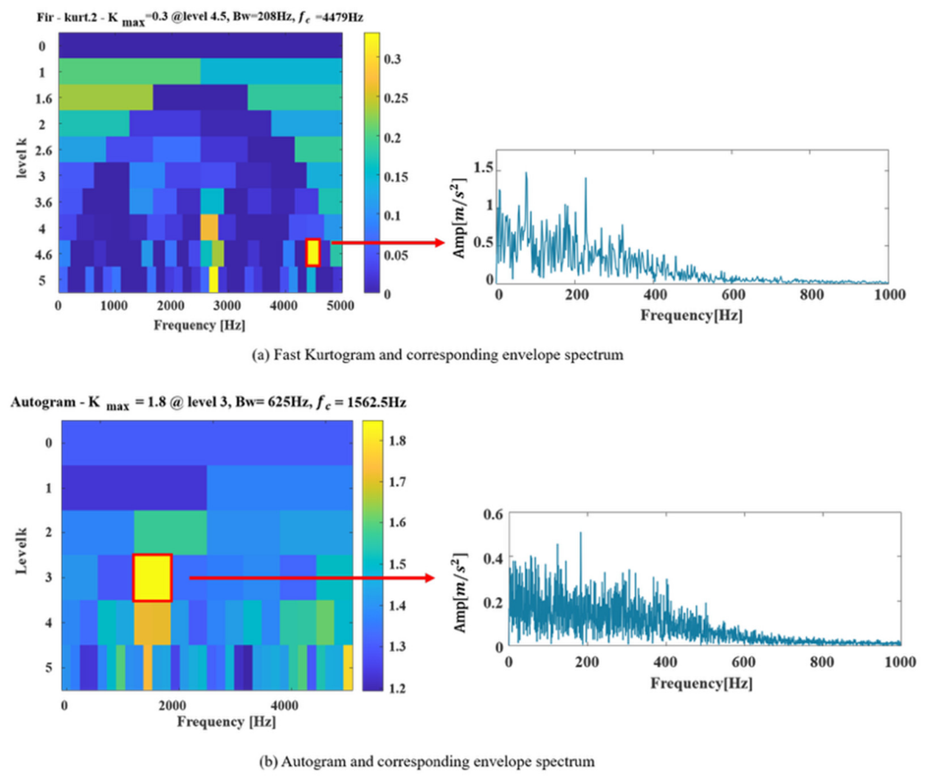
Under the same experimental conditions, all three methods were applied to process and analyze the vibration signal of the bearing outer ring fault to clearly highlight the superiority of the AFGS Model in fault feature extraction and diagnosis accuracy. As shown in Figure 17. The Fast Kurtogram located the fault at the 4.6 decomposition level (center frequency , bandwidth ), but the reconstructed signal envelope spectrum did not show any fault characteristic frequencies, rendering the diagnosis ineffective. The Autogram algorithm located the optimal sensitive fault band at the 3rd decomposition level, with a corresponding center frequency of and an effective bandwidth of , but also failed to identify any valid fault information after reconstruction. Both the Fast Kurtogram and Autogram algorithms failed to realize accurate diagnosis of this bearing fault due to ineffective feature extraction. These limitations of the two conventional methods fully reflect the outstanding performance and inherent superiority of the proposed AFGS Model.
Figure 17.
The envelope spectrum obtained using the Fast Kurtogram and Autogram methods.
5.2. Bearing Inner Ring Test Signals
This section presents a systematic analysis of the vibration signal collected from the bearing inner ring fault. All experimental vibration data used in the research were obtained from the professional bearing fault test platform displayed on Figure 18. The tested bearing model was 6205, for which the inner ring fault characteristic frequency was theoretically calculated to be . The studied fault type in this case is a typical bearing inner ring crack defect, as clearly illustrated in Figure 18a. Meanwhile, the original time-domain vibration signal collected from the bearing with inner ring failure is presented in Figure 18b for subsequent comparative analysis. Due to the heavy background noise in the experimental environment, the periodic fault impulse signals generated by the inner ring crack in the time-domain waveform were completely masked and could not be effectively identified. In the corresponding Hilbert envelope spectrum of the original signal, only the rotational frequency (denoted as ) could be barely distinguished, and this frequency component was significantly affected by noise interference, resulting in blurred spectral peaks and difficulty in extracting effective fault characteristic information. No characteristic frequency components related to the inner ring fault appeared. Further fault information needs to be extracted through professional signal processing methods.
Figure 18.
Inner ring fault and inner ring experimental signal.
The proposed AFGS Model was used to process the inner ring fault signal, and the results are shown in Figure 19. By extracting the signal feature value information, the key node was determined to be 2372, and the corresponding key frequency-domain spectrum band was obtained. Combined with the CSNE index evaluation results shown in Figure 19b, and by analyzing the index distribution across different frequency bands, the optimal order band corresponding to the maximum CSNE value was determined to be . This optimal order band was extracted, and the time-domain signal was reconstructed by the inverse graph Fourier transform, with the results shown in Figure 20. The reconstructed time domain waveform showed significant periodic pulse characteristics. The Hilbert envelope spectrum not only clearly displayed the 2-fold rotational frequency component, but also distinctly revealed the third harmonic component of the inner ring fault characteristic frequency with negligible noise interference. In addition, Figure 20b presents a local waveform comparison between the original noisy signal and the reconstructed signal within the time interval of , which intuitively reflects the prominent denoising and feature enhancement effect of the proposed method. It can be clearly observed that the average pulse interval of the reconstructed time-domain signal was approximately . This time interval corresponds well and is highly consistent with the theoretical characteristic frequency of the bearing inner ring fault . The excellent agreement between the experimental result and theoretical value further verifies that the AFGS Model has outstanding accuracy and reliability in extracting hidden weak fault feature information from noisy vibration signals.
Figure 19.
AFGS Model processing results of inner ring signal.
Figure 20.
Time-domain waveforms and envelope spectra obtained using the AFGS Model.
To further demonstrate the performance advantages of the method proposed in this work, two well-established mainstream algorithms were selected for comparative evaluation under the same test conditions. Specifically, the Fast Kurtogram and Autogram algorithms were selected for comparative experiments. The results obtained by the Fast Kurtogram algorithm are illustrated in Figure 21a. The algorithm identified the potential fault-related frequency band at the 5th decomposition level, with a center frequency of and a bandwidth of . While this band did contain some fault-related information, no distinct periodic impulses were observed in the reconstructed time-domain signal, and the corresponding envelope spectrum only showed the 1st and 2nd harmonics of the rotational frequency. Moreover, the reconstructed signal was severely affected by noise interference and failed to achieve effective fault diagnosis. The output results of the Autogram algorithm are presented in Figure 21b. The fault frequency band detected by this algorithm had a center frequency of 768 Hz and a bandwidth of 512 Hz, with an extremely low proportion of effective fault information within this range. The reconstructed time-domain waveform failed to exhibit any obvious periodic fault impulses. Meanwhile, the Hilbert envelope spectrum of this signal only revealed the 2nd harmonic of the shaft rotational frequency, with no clear fault characteristic components detected. Similarly, this algorithm failed to effectively extract the inner ring fault features. In summary, neither the Fast Kurtogram nor the Autogram algorithm could accurately diagnose the inner ring fault signal, while the AFGS Model method, with its optimized frequency-domain spectral modeling and adaptive frequency band selection strategy, demonstrated superior fault feature extraction capabilities and noise resistance.
Figure 21.
Envelope spectrum obtained using the Fast Kurtogram and Autogram methods.
Table 1 shows the single computation time of three algorithms—AFGS, Fast Kurtogram, and Autogram—for three datasets: simulation signal, bearing outer ring, and bearing inner ring.
Table 1.
Comparison of computation time for different algorithms.
The time consumption results show that the AFGS Model in this paper adopts a binary iterative search strategy, which had logarithmic time complexity and a lower computation time than Fast Kurtogram and Autogram. Autogram had the highest computational cost due to nested autocorrelation operations. Combined with the fault feature extraction effect, AFGS has comprehensive advantages in fault identification capability and computational efficiency.
6. Conclusions
To address the issue that bearing fault characteristics in rotating machinery are easily obscured by strong noise, and that traditional diagnostic methods suffer from fixed graph topology, reliance on human experience, and insufficient anti-interference capabilities, this paper proposes an adaptive frequency spectrum model (AFGS Model) for bearing fault diagnosis.
This paper addresses the problems of easily masked fault features in rotating machinery bearings under strong noise backgrounds and the reliance on manual experience and insufficient noise resistance of traditional diagnostic methods. Based on graph signal processing theory, a novel bearing fault diagnosis method, the adaptive frequency graph spectrum model (AFGS Model), is proposed, effectively solving the problem of poor fault feature extraction when directly converting time-domain signals to the spectral domain for analysis. The proposed method first transforms the raw vibration signal from the time domain into the frequency domain using the fast Fourier transform (FFT) while retaining the complete phase information during the entire conversion process. Subsequently, the amplitude sequence obtained from the FFT output is utilized to construct a graph signal. This graph signal is then systematically represented in matrix form, allowing the corresponding Laplace matrix to be derived. At the same time, eigenvalue decomposition is performed on the constructed matrix, yielding the feature sequence along with its corresponding eigenvectors. Based on the resulting feature sequence, key nodes in the graph signal are then identified, which serve as the basis for subsequent screening in the frequency domain. After screening key frequency-domain nodes, the last 128 nodes are selected as the core analysis interval. The bisection adaptive search strategy and the CSNE evaluation indicator are combined to lock the optimal fault feature order band. Finally, accurate fault diagnosis is achieved through signal reconstruction and envelope spectrum calculation. The CSNE indicator, with its high sensitivity to periodic impacts and strong noise resistance, provides a reliable quantitative basis for frequency band selection, while the bisection method improves the efficiency and automation level of diagnosis with logarithmic computational complexity.
Cross-comparison of the simulation and experimental results show that under the simulation condition of −3 dB strong noise, AFGS could completely extract the 1st to 8th order harmonics of bearing faults while Fast Kurtogram and Autogram could only identify a small number of low-order harmonics. Under the strong noise fault signals of the outer and inner races measured on the bench, the two comparative algorithms completely failed and could not detect the fault features, while AFGS could still clearly identify the fault characteristic frequencies and their multiple harmonics. At the same time, the calculation time results show that thanks to the logarithmic time complexity of the bisection framework, AFGS has a lower average computation time than Fast Kurtogram and Autogram and has advantages in both fault identification capability and computational efficiency.
The following solutions address the existing technical challenges raised in the introduction. By dynamically constructing graph signals in the frequency domain, the constraints of traditional fixed graph topologies are eliminated, allowing adaptation to time-varying bearing fault characteristics; fully data-driven order-band optimization is achieved using a bipartite framework and the CSNE index, eliminating reliance on human experience and prior fault parameters; the CSNE index enhances periodic impact characteristics and suppresses random noise interference, significantly improving the ability to extract weak early faults under strong noise environments; and multi-scale fault features of the graph are automatically mined, reducing feature redundancy.
The main innovations of this paper are summarized as follows:
- (1)
- A novel approach to frequency-domain mapping is proposed. Unlike the traditional method of directly constructing a fixed topology map from time-domain vibration signals, this approach constructs a map signal based on FFT amplitude sequences, preserving the original phase for signal reconstruction. This avoids noise interference during the mapping stage and overcomes the limitation of fixed map topologies being difficult to adapt to time-varying faults.
- (2)
- A correlation spectrum negative entropy (CSNE) evaluation index is proposed. This index utilizes the autocorrelation characteristics of fault impacts, and compared to traditional indices such as kurtosis, is more sensitive to periodic fault impacts and has stronger resistance to random noise and accidental pulse interference.
- (3)
- Fast binary search is introduced into the optimal fault order band selection, replacing the traditional sliding window traversal strategy. This achieves automatic search for the optimal fault order band without manual intervention with logarithmic complexity, balancing computational efficiency and the degree of diagnostic automation.
Simulation signal verification and experimental data processing of wind turbine bearing inner and outer ring faults both demonstrate that the proposed AFGS Model method can effectively extract the periodic impact characteristics of bearing faults under strong noise environments. The envelope spectrum of the reconstructed signal can clearly present the multiple harmonic information of the fault characteristic frequency without significant noise interference. Compared with traditional fault diagnosis algorithms such as Fast Kurtogram and Autogram, this method shows significant advantages in the accuracy of fault frequency band localization, noise suppression capability, and completeness of fault feature extraction. The proposed method provides an efficient and reliable new method for bearing condition monitoring and fault diagnosis of rotating machinery under complex working conditions.
Future work outlook: The current AFGS Model primarily focuses on single-type bearing faults under constant speed conditions. Future research will further expand the algorithm by combining order tracking and angle resampling techniques to address fault diagnosis issues under highly non-stationary conditions of variable speed wind turbines and under conditions of extremely low fundamental frequency of the main shaft; conducting research on the separation and identification of composite bearing faults; optimizing the hyperparameter adaptive selection strategy to avoid empirical settings for a fixed number of intercepted nodes; and deploying the algorithm to edge devices for engineering-level testing in the online monitoring of wind turbines.
Author Contributions
Writing—original draft preparation, Conceptualization, P.X.; Methodology, Software, Y.L.; Formal analysis, investigation, H.Z.; Validation, Resources, Data curation, Y.Y.; Writing—review and editing, Visualization, D.L.; Project administration, Funding acquisition, Y.X.; Supervision, L.F. All authors have read and agreed to the published version of the manuscript.
Funding
This research was funded by the CGN (Beijing) New Energy Technology Co., Ltd. research project (S-Y2025DBN).
Data Availability Statement
The data presented in this study are available on request from the corresponding author.
Acknowledgments
The authors would like to gratefully acknowledge the CGN (Beijing) New Energy Technology Co., Ltd. research project (S-Y2025DBN).
Conflicts of Interest
Author Peng Xu, Yiding Liu, Huaming Zhang, Yousheng Yang, Dian Liu, Yonggang Xu, Lei Feng, were employed by the company CGN (Beijing) New Energy Technology. The authors declare that the research was conducted in the absence of any commercial or financial relationships that could be construed as a potential conflict of interest.The authors declare that this study received funding from CGN (Beijing) New Energy Technology Co., Ltd. research project (S-Y2025DBN). The founder had the following involvement with the study: research design, data collection, data analysis, data interpretation, manuscript writing, or the decision to submit for publication.
References
- Bao, W.; Liu, S.; Liu, Z.; Li, F. Generalized synchroextracting transform: Algorithm and applications. Mech. Syst. Signal Process. 2025, 224, 112116. [Google Scholar] [CrossRef] [Scilit]
- Shao, Z.; Jiang, H.; Zhang, X.; Zhou, J.; Huang, W. PLL-WCAN: Pseudo-label progressive learning guided wavelet class-aware adaptive network for gearbox cross-domain fault diagnosis. Mech. Syst. Signal Process. 2025, 230, 112624. [Google Scholar] [CrossRef] [Scilit]
- Ge, L.; Zhao, D.; Wang, T.; Cui, L. High-dimensional optimized extraction chirplet transform: Algorithm and applications. ISA Trans. 2026, 169, 520–534. [Google Scholar] [CrossRef] [Scilit] [PubMed]
- Yuan, R.; Liu, H.; Lv, Y.; Chen, Y.; Yang, X.; Li, H.; Chelidze, D. Ball tree structure-informed phase space warping: A robust algorithm for dynamic degradation tracking under variable speed conditions. Adv. Eng. Inform. 2026, 71, 104288. [Google Scholar] [CrossRef] [Scilit]
- Chen, J.; Xu, Y.; Liu, T.; Yang, M.; Zhang, K.; Zhang, H. A convex optimization difference analysis model for intelligent fault detection and diagnosis of gearboxes. Mech. Syst. Signal Process. 2026, 251, 114207. [Google Scholar] [CrossRef] [Scilit]
- Qin, Y. A new family of model-based impulsive wavelets and their sparse representation for rolling bearing fault diagnosis. IEEE Trans. Ind. Electron. 2018, 65, 2716–2726. [Google Scholar] [CrossRef] [Scilit]
- Peng, Y.; Shao, H.; Yan, S.; Wang, J.; Xiao, Y.; Liu, B. A systematic review on interpretability research of intelligent fault diagnosis models. Meas. Sci. Technol. 2025, 36, 012009. [Google Scholar] [CrossRef] [Scilit]
- Chen, D.; Qin, Y.; Wang, Y.; Zhou, J. Health indicator construction by quadratic function-based deep convolutional auto-encoder and its application into bearing RUL prediction. ISA Trans. 2021, 114, 44–56. [Google Scholar] [CrossRef] [Scilit] [PubMed]
- Huangfu, Y.F.; Chen, K.K.; Ma, H.; Li, X.; Han, H.Z.; Zhao, Z.F. Meshing and dynamic characteristics analysis of spalled gear systems: A theoretical and experimental study. Mech. Syst. Signal Process. 2020, 139, 106640. [Google Scholar] [CrossRef] [Scilit]
- Huangfu, Y.F.; Dong, X.J.; Yu, X.L.; Chen, K.K.; Li, Z.W.; Peng, Z.K. Fault tracing of gear systems: An in-situ measurement-based transfer path analysis method. J. Sound Vib. 2023, 553, 117610. [Google Scholar] [CrossRef] [Scilit]
- Shi, J.; Moura, J.M.F. Topics in graph signal processing: Convolution and modulation. In Proceedings of the 2019 53rd Asilomar Conference on Signals, Systems, and Computers, Pacific Grove, CA, USA, 3–6 November 2019; pp. 457–460. [Google Scholar]
- Hammond, D.K.; Vandergheynst, P.; Gribonval, R. Wavelets on graphs via spectral graph theory. Appl. Comput. Harmon. Anal. 2011, 30, 129–150. [Google Scholar] [CrossRef] [Scilit]
- An, X.; Jiang, D.; Chen, J.; Liu, C. Application of the intrinsic time-scale decomposition method to fault diagnosis of wind turbine bearing. J. Vib. Control 2012, 18, 240–245. [Google Scholar] [CrossRef] [Scilit]
- Ou, L.; Yu, D. Fault diagnosis of roller bearings based on Laplacian energy feature extraction of path graphs. Measurement 2016, 94, 168–176. [Google Scholar] [CrossRef] [Scilit]
- Furutani, S.; Shibahara, T.; Akiyama, M.; Hato, K.; Aida, M. Graph signal processing for directed graphs based on the Hermitian Laplacian. In Proceedings of the European Conference Machine Learning and Knowledge Discovery in Databases (ECML PKDD), Würzburg, Germany, 16–20 September 2019; pp. 447–463. [Google Scholar]
- Ruiz, L.; Chamon, L.F.O.; Ribeiro, A. Graphon signal processing. IEEE Trans. Signal Process. 2021, 69, 4961–4976. [Google Scholar] [CrossRef] [Scilit]
- Tang, Z.; Wang, M.; Ouyang, T.; Che, F. A wind turbine bearing fault diagnosis method based on fused depth features in time-frequency domain. Energy Rep. 2022, 8, 12727–12739. [Google Scholar] [CrossRef] [Scilit]
- Dhamande, L.S.; Chaudhari, M.B. Compound gear-bearing fault feature extraction using statistical features based on time-frequency method. Measurement 2018, 125, 63–77. [Google Scholar] [CrossRef] [Scilit]
- Hou, J.; Wu, Y.; Ahmad, A.S.; Gong, H.; Liu, L. A novel rolling bearing fault diagnosis method based on adaptive feature selection and clustering. IEEE Access 2021, 9, 100309–100320. [Google Scholar] [CrossRef] [Scilit]
- Sun, Y.; Yu, J. Adaptive sparse representation-based minimum entropy deconvolution for bearing fault detection. IEEE Trans. Instrum. Meas. 2021, 70, 3513010. [Google Scholar] [CrossRef] [Scilit]
- Hu, G.; Gu, B.; Yang, L.; Wu, S.; Zhao, P. Spectrum sensing based on graph Fourier transform using Laplacian matrix and vertex probability vector. IEEE Trans. Commun. 2024, 72, 2579–2593. [Google Scholar]
- Usta, Ö.C.; Akay, O. Definition of a graph cepstrum for homomorphic processing of graph signals. In Proceedings of the 31st Signal Processing and Communications Applications Conference (SIU), Istanbul, Turkiye, 5–8 July 2023; pp. 1–4. [Google Scholar]
- Liu, Z.; Zhang, L. A review of failure modes, condition monitoring and fault diagnosis methods for large-scale wind turbine bearings. Measurement 2020, 149, 107002. [Google Scholar] [CrossRef] [Scilit]
- Wei, D.; Yuan, S. Hermitian random walk graph Fourier transform for directed graphs and its applications. Digit. Signal Process 2024, 155, 104742. [Google Scholar] [CrossRef] [Scilit]
- Shi, L.; Fan, J.Y.; Xu, Y.G.; Wang, X.H.; Zhang, K.; Zhang, H.M.; Liu, Y.F. Targeted diagnosis via spectral modulation Fourier decomposition for bearing faults. Sci. China Technol. Sci. 2026. just accepted. [Google Scholar] [CrossRef]
- Antoni, J. Fast computation of the kurtogram for the detection of transient faults. Mech. Syst. Signal Process. 2007, 21, 108–124. [Google Scholar] [CrossRef] [Scilit]
- Moshrefzadeh, A.; Fasana, A. The Autogram: An effective approach for selecting the optimal demodulation band in rolling element bearings diagnosis. Mech. Syst. Signal Process. 2018, 105, 294–318. [Google Scholar] [CrossRef] [Scilit]
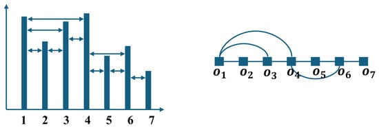
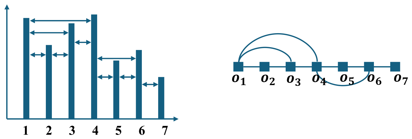
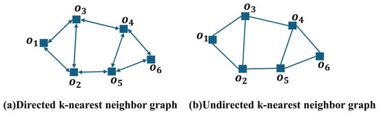
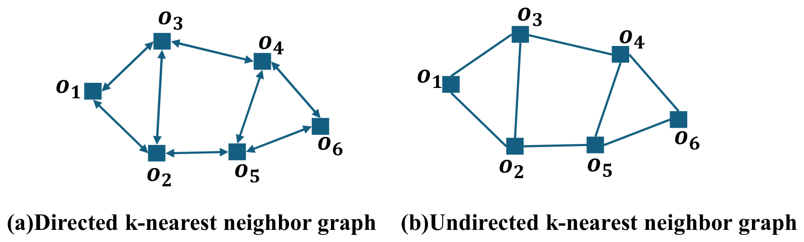
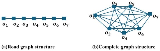
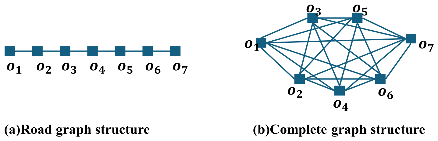
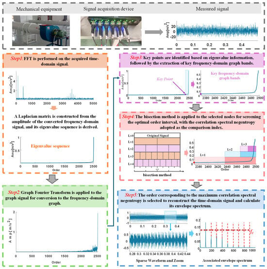
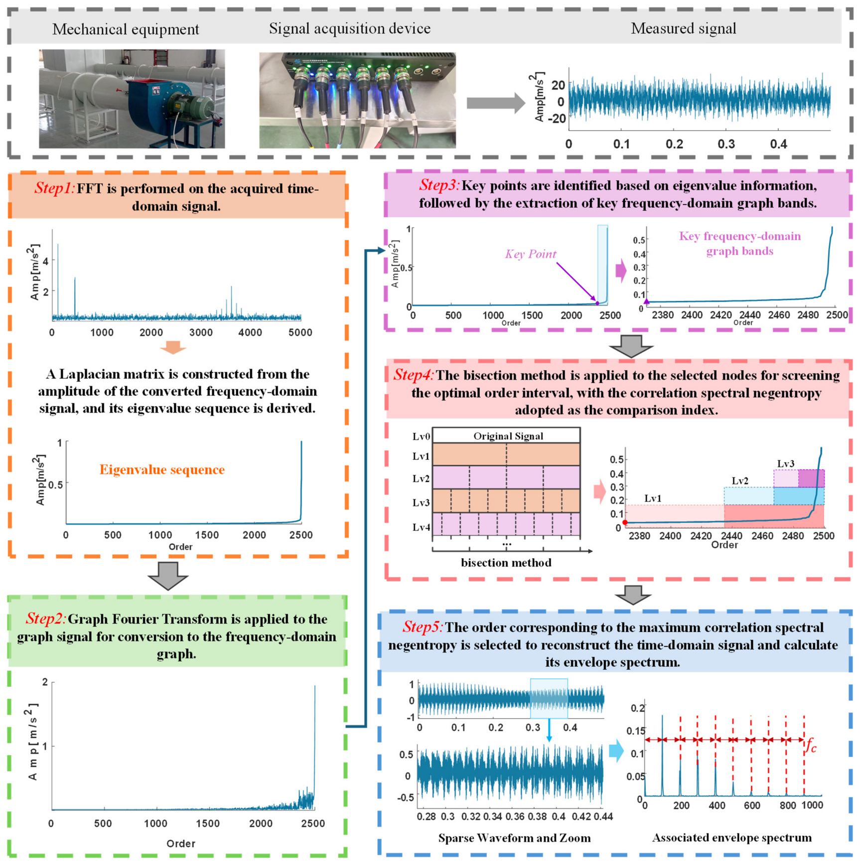
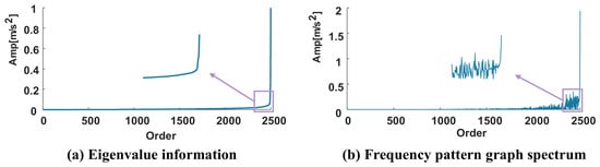
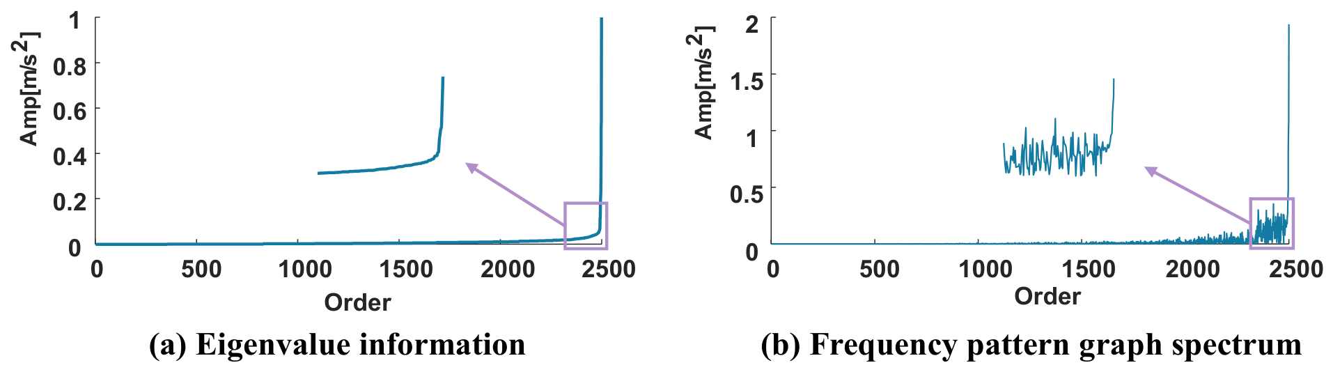
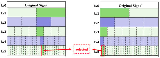
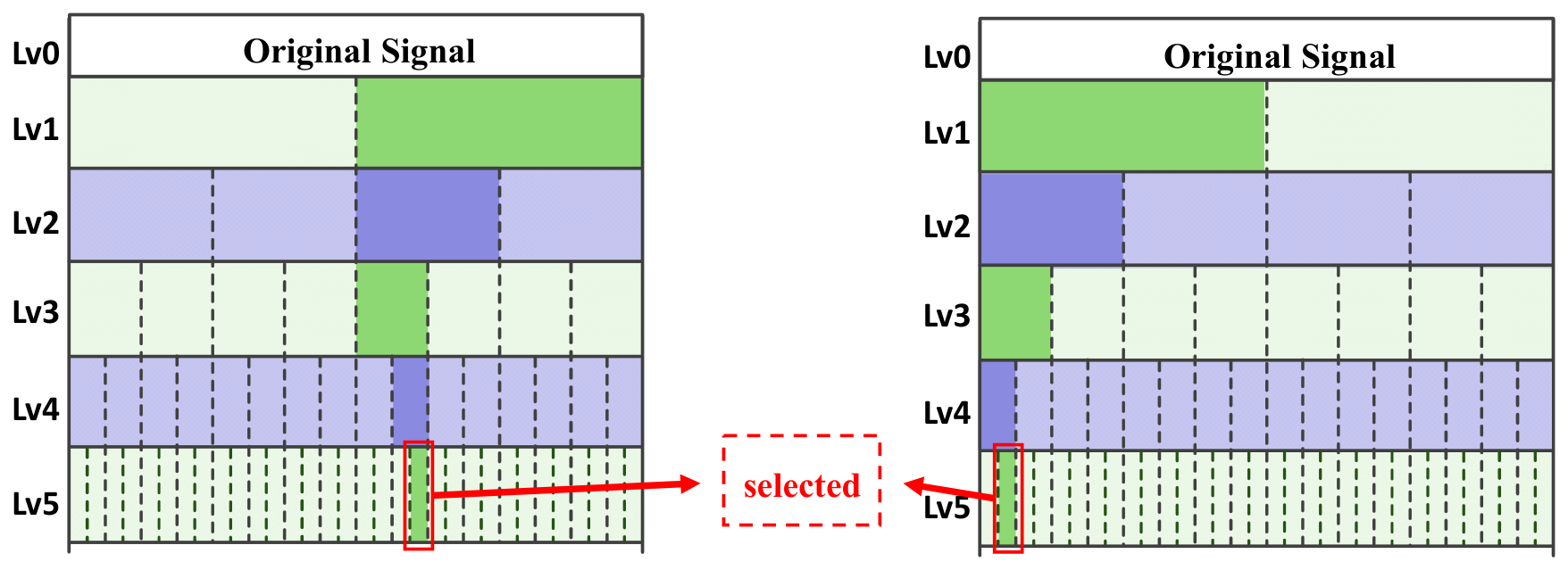
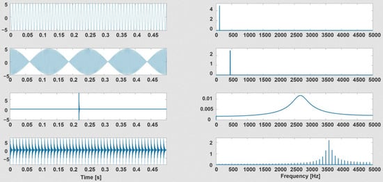
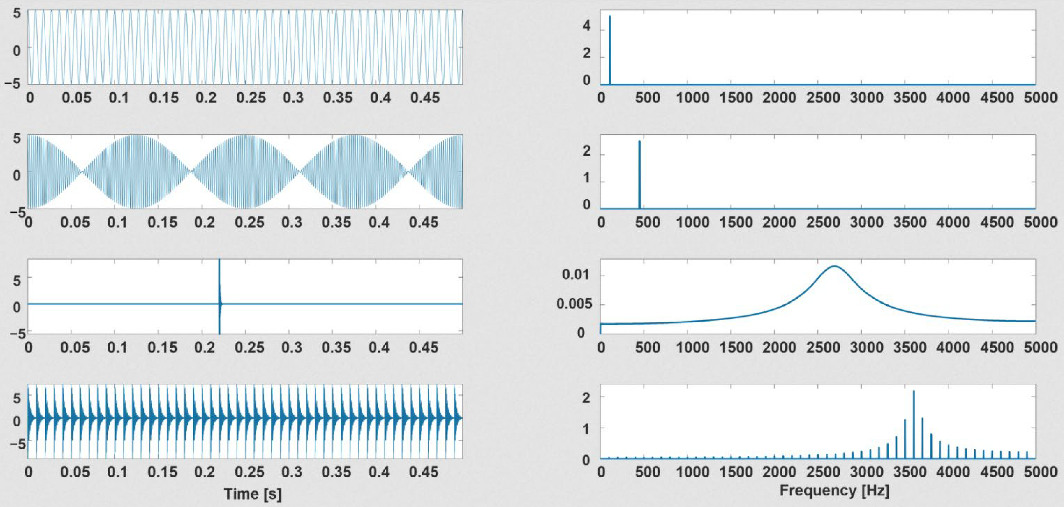
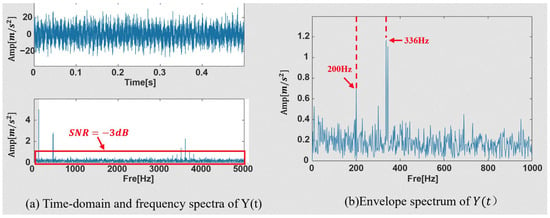
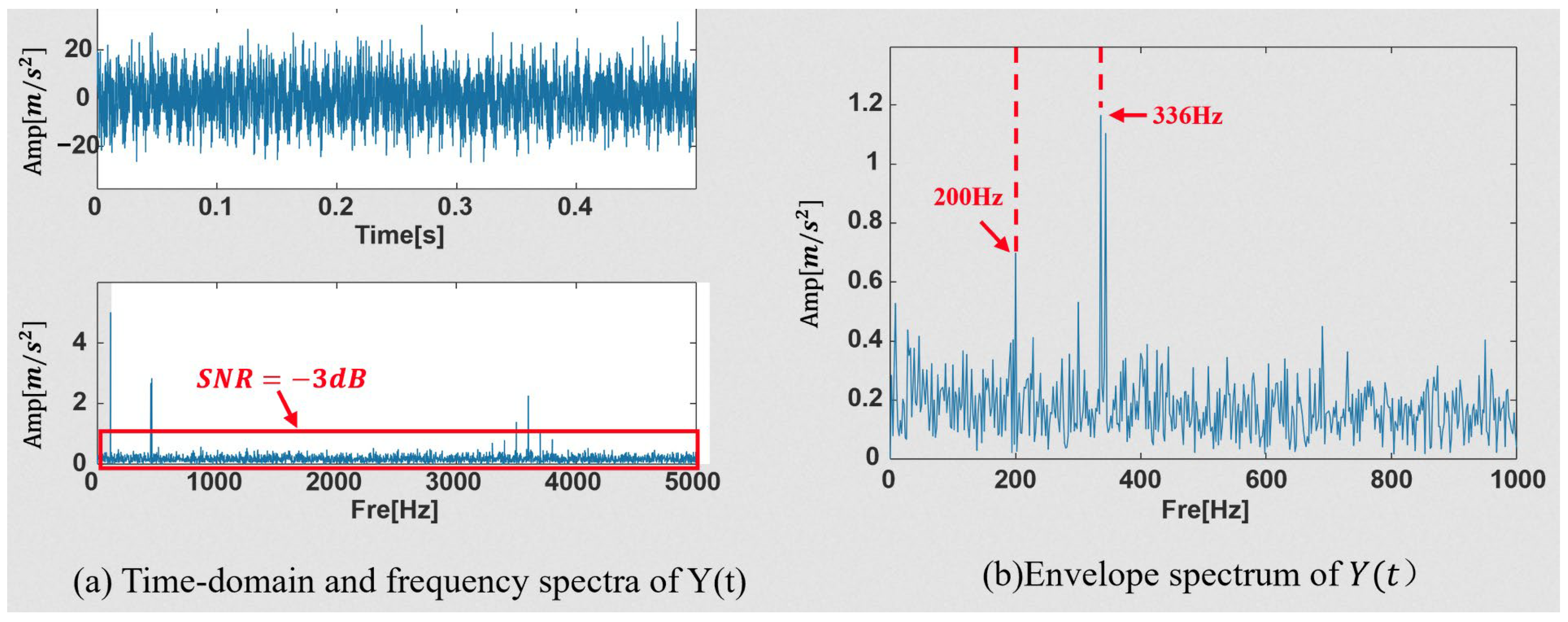
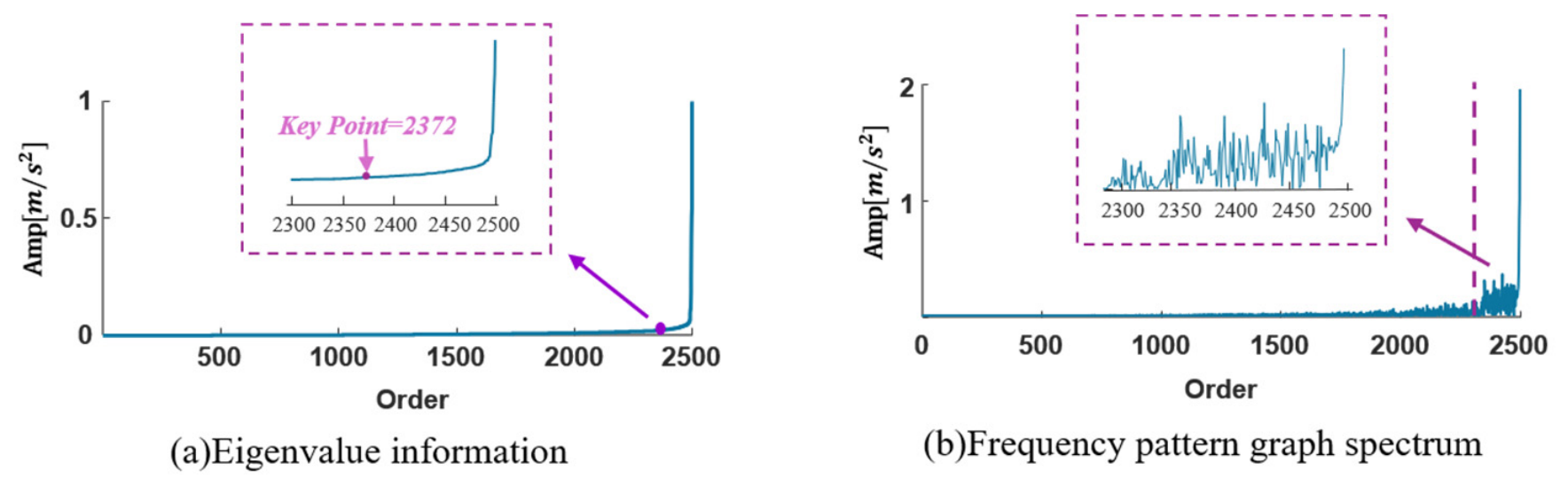
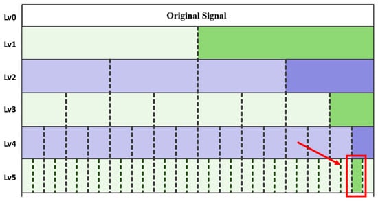
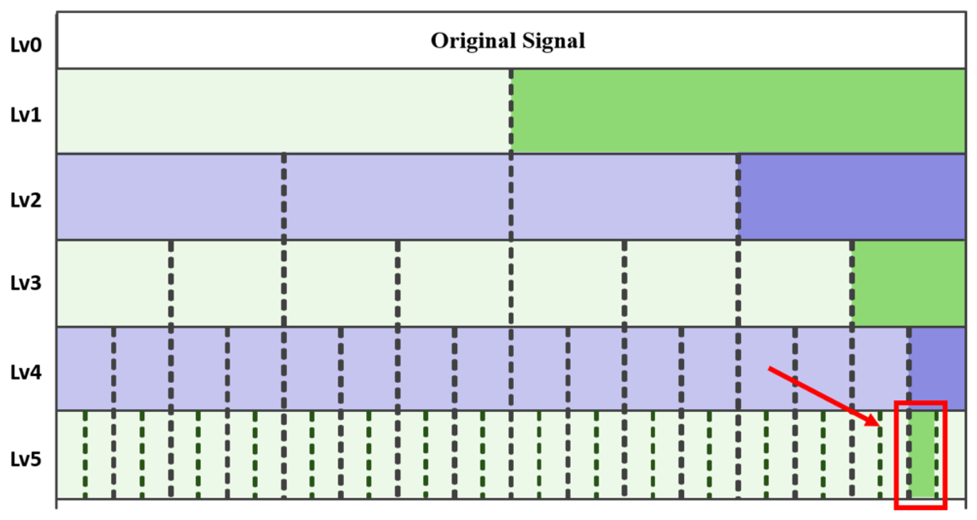
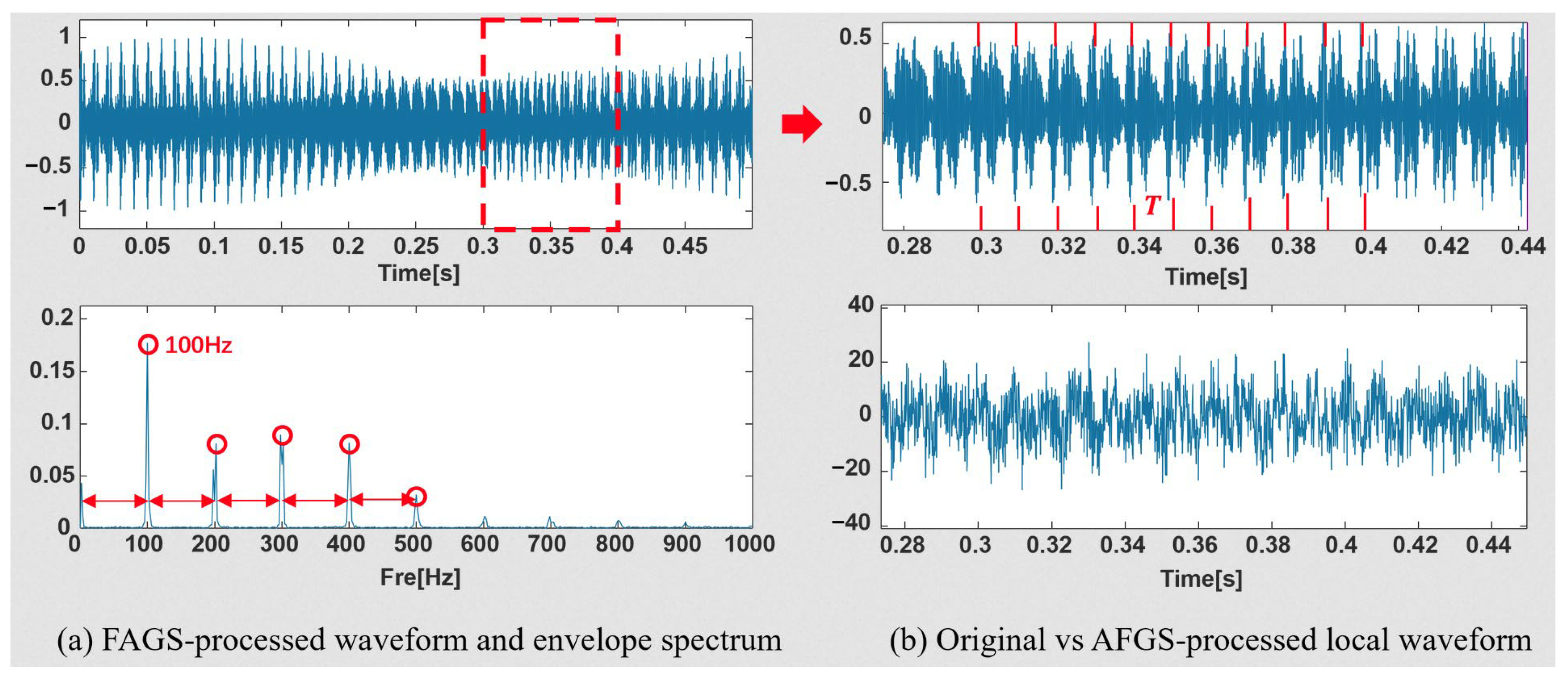
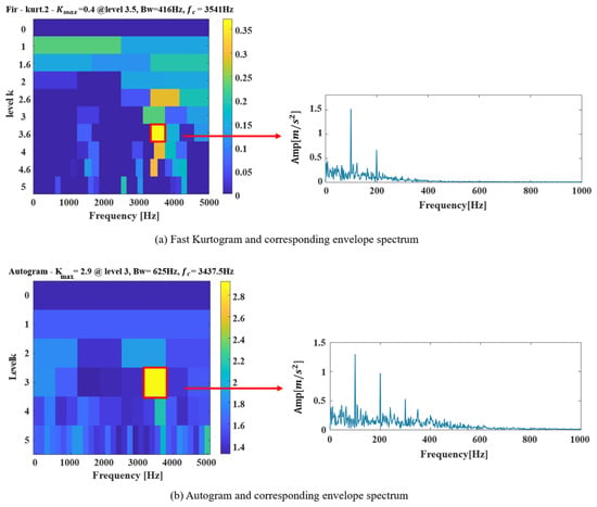
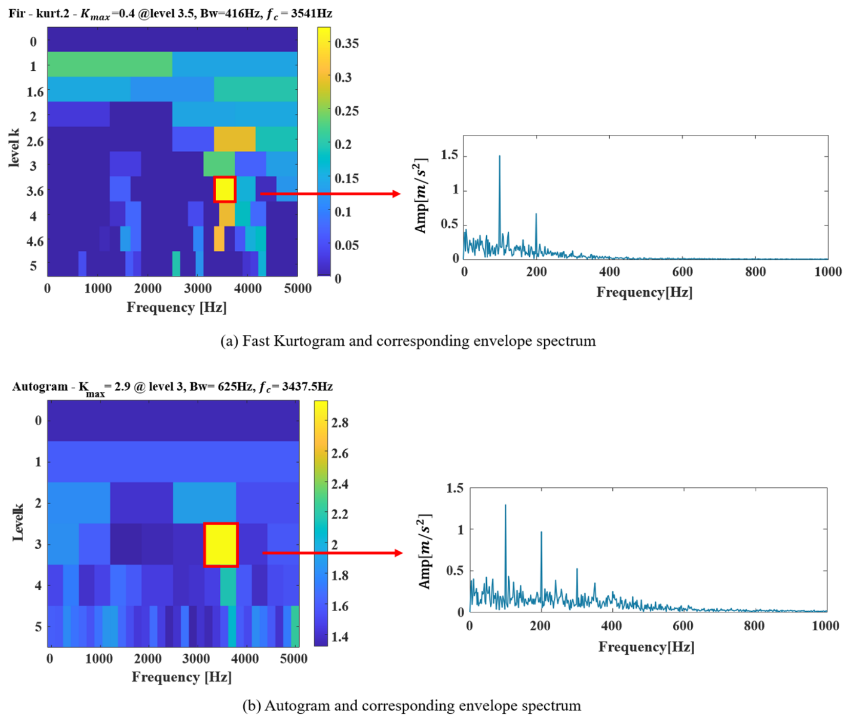
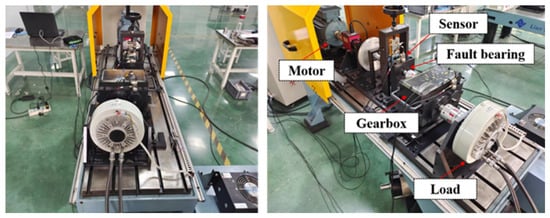
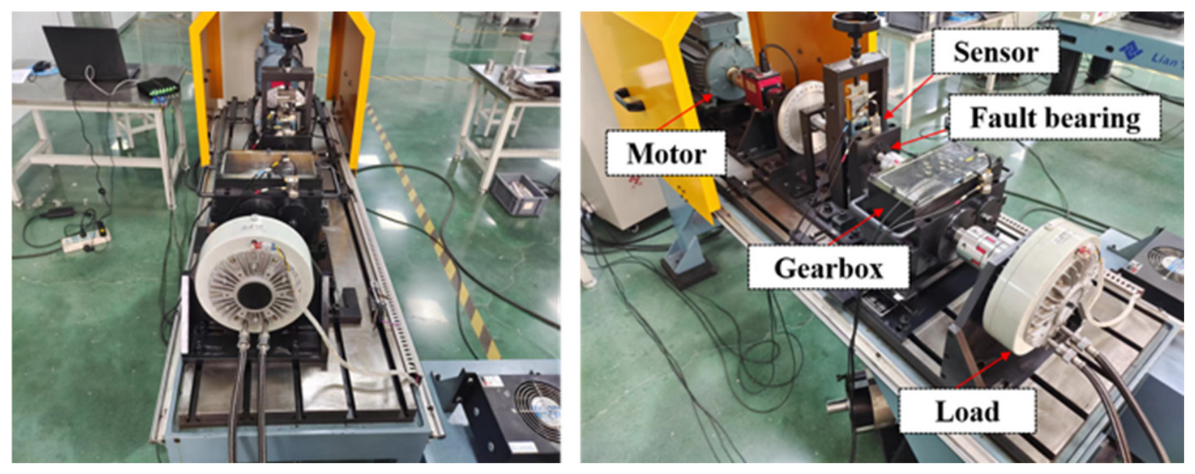
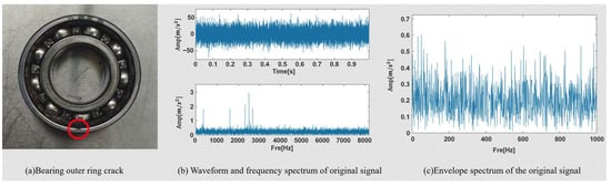
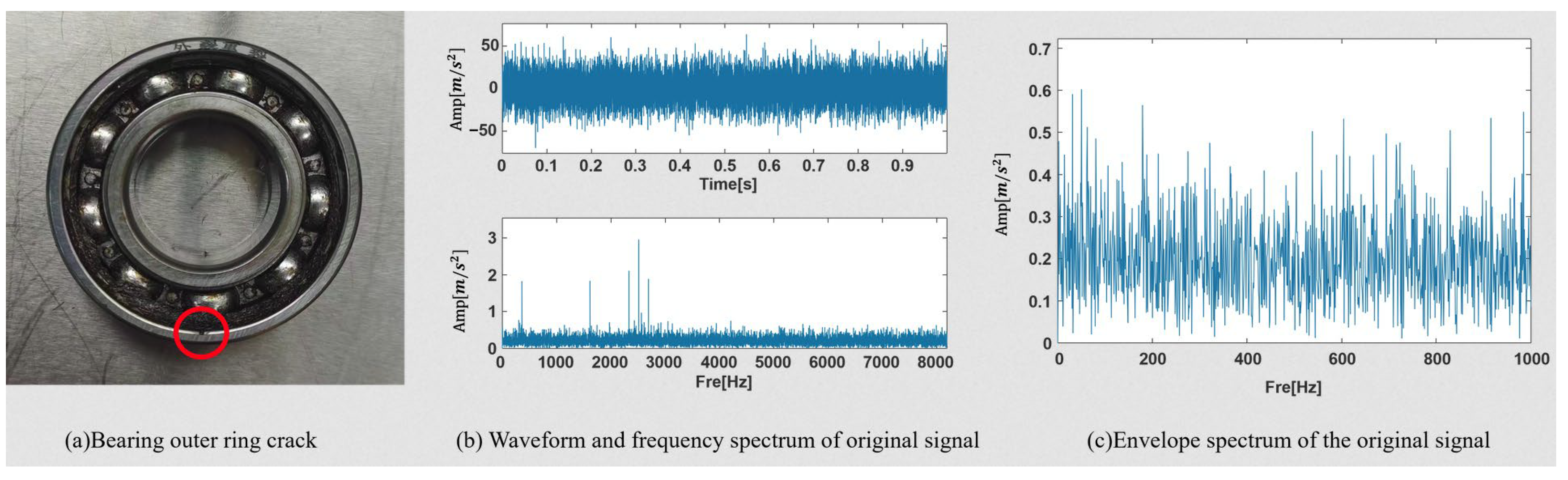
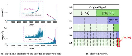
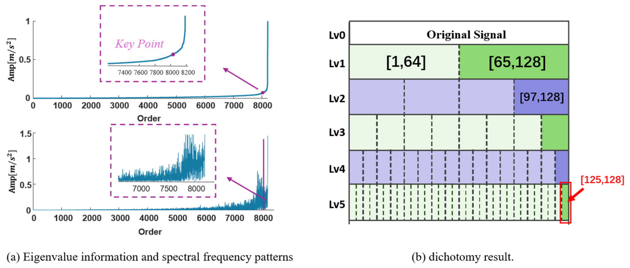
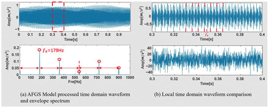
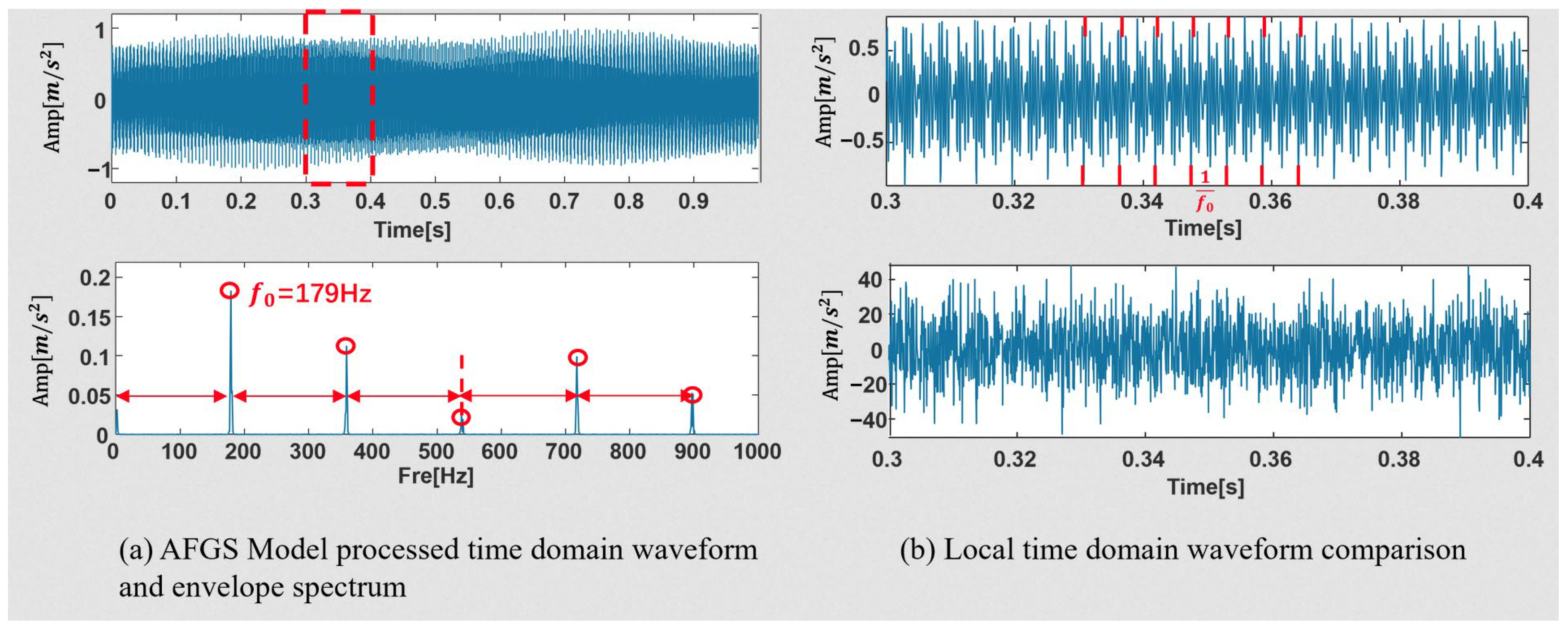
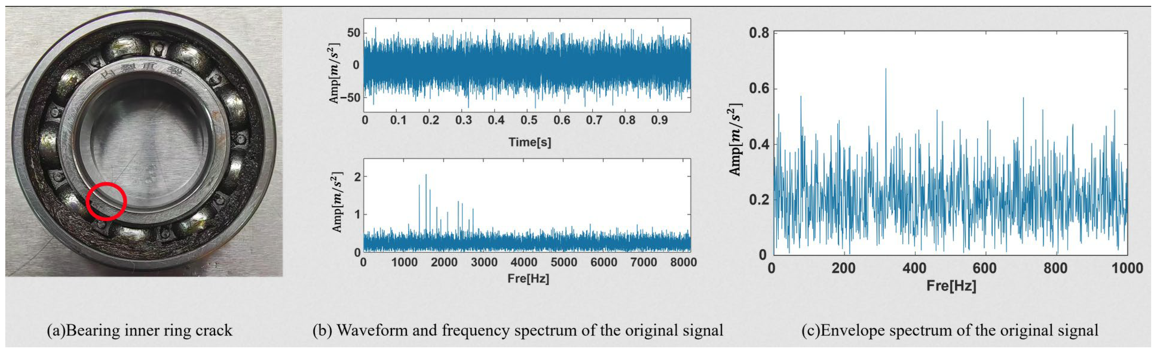
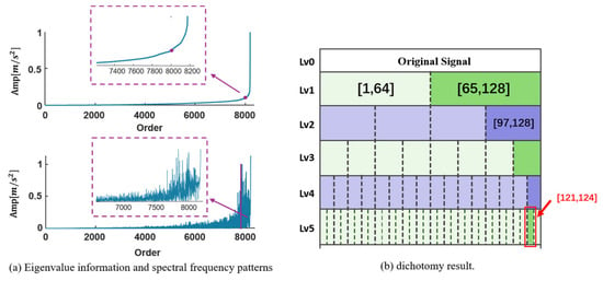
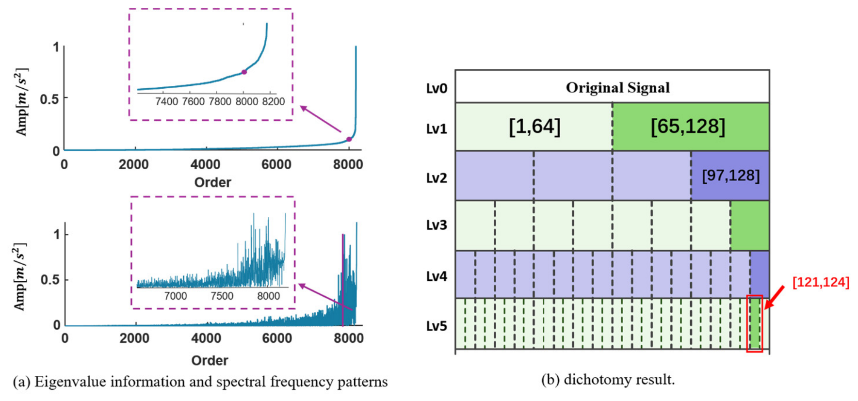
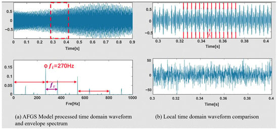
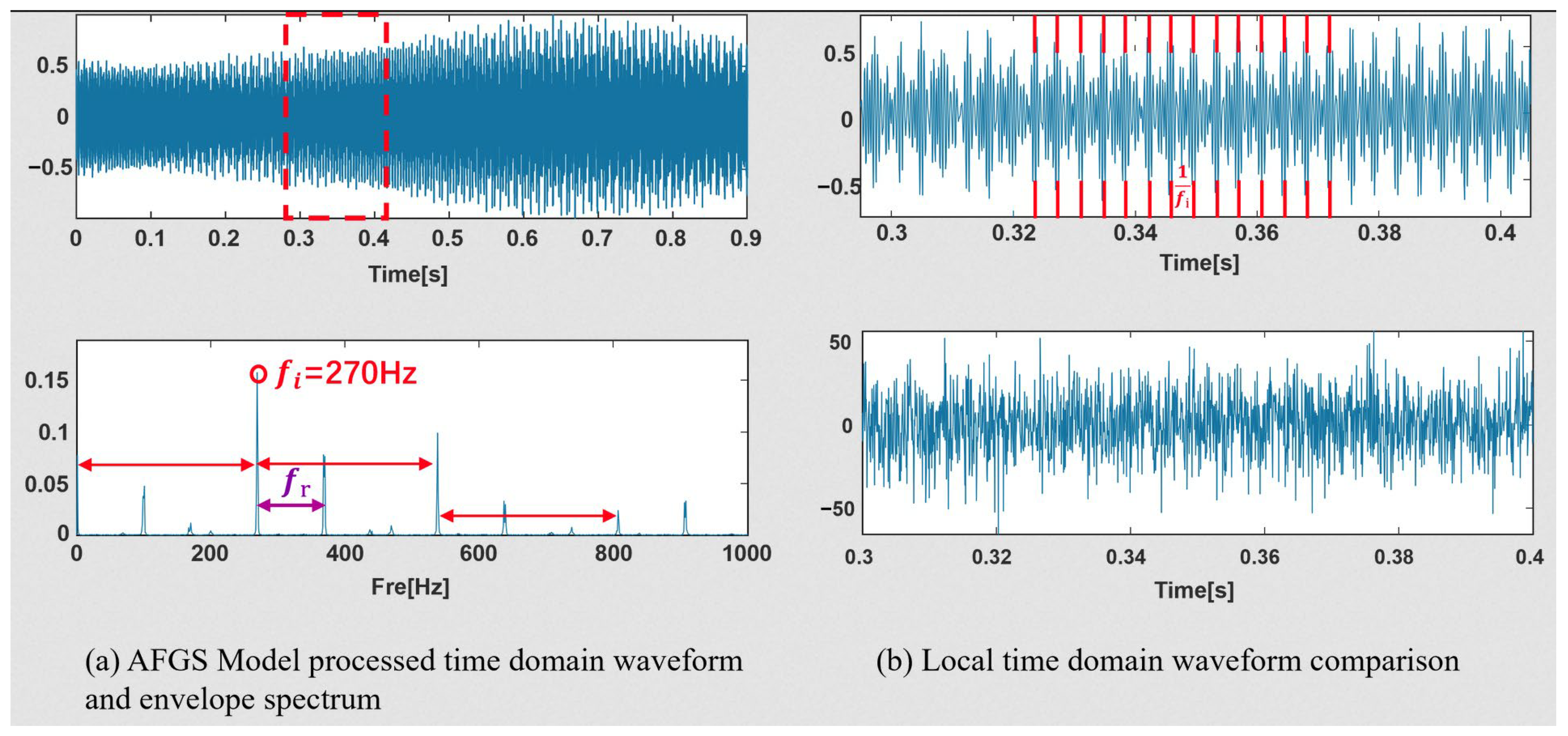
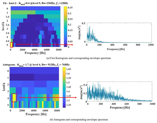
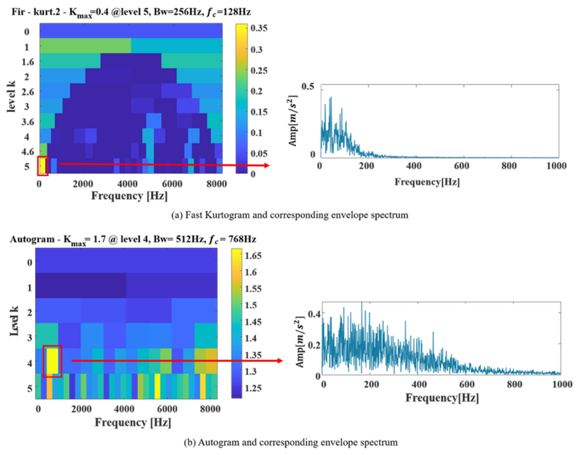

Disclaimer/Publisher’s Note: The statements, opinions and data contained in all publications are solely those of the individual author(s) and contributor(s) and not of MDPI and/or the editor(s). MDPI and/or the editor(s) disclaim responsibility for any injury to people or property resulting from any ideas, methods, instructions or products referred to in the content. |
© 2026 by the authors. Licensee MDPI, Basel, Switzerland. This article is an open access article distributed under the terms and conditions of the Creative Commons Attribution (CC BY) license.