LEADI: Operating-Mode-Aware Machine Condition Monitoring for Leak-Related Energy Anomalies—A Before-and-After Maintenance Study of a Single Production Asset

Abstract

Compressed-air leaks create persistent parasitic demand, but machine-level condition monitoring is difficult because air consumption changes strongly with operating mode. LEADI (Leak Energy Anomaly Detection Index) was developed as an operating-mode-aware procedure that evaluates the deviation of directly measured flow rate from a local reference baseline derived from a stable post-repair condition with maintained pressure and low within-window variability. The method was developed on days 1–5 and evaluated on held-out days 6–7 from two one-week campaigns conducted before and after implementation of the prescribed corrective actions. With 60 min windows, LEADI flagged 19/19 evaluable pre-repair and 0/17 post-repair windows, with diagnostic coverage of 39.6% and 35.4%, respectively. A simple fifth-percentile flow comparator without operating-mode selection flagged 47/48 versus 1/48 windows. This shows that the low-flow region itself contains strong discriminatory information for separating the two periods. The role of the operating-mode layer is to restrict engineering interpretation to pre-specified eligible operating conditions. The flow-rate difference within the diagnostic operating condition was 122.0 L/min (95% CI 114.6–132.3). Over a common 168 h basis, measured volume decreased by 1370.8 m³ (28.90%), while a separate check normalized by pressurized time gave 28.12%. Because the specific energy consumption of the compressor station was not measured, the energy effect is reported only as a scenario for the same 168 h. The results support the applicability of LEADI as a selective decision-support layer for the investigated asset and the two observed conditions, without establishing universal leak detection or causal attribution of the observed change to individual defects.

1. Introduction

Compressed-air systems are among the least energy-efficient utility systems used in automated manufacturing. They remain widespread because they are simple, reliable, clean, safe in hazardous environments, and easy to integrate into cyclic machinery. These advantages come at a substantial energy cost. Energy is lost during compression, cooling, drying, filtration, distribution, pressure regulation, and throttling, and only part of the supplied electrical energy is ultimately converted into useful mechanical work. Compressed air should therefore not be treated as an inexpensive auxiliary utility, but as a costly secondary energy carrier that affects operating costs, carbon emissions, and production reliability [1,2,3]. In highly automated plants, pneumatic systems often remain pressurized while individual machines move between production, standby, cleaning, and intermediate process states. Continuous pressurization allows even small defects to create persistent losses. A leak that appears minor during a spot inspection can sustain parasitic flow for weeks or months. Leakage losses are commonly estimated at 20–30% of compressed air supplied and may be higher in poorly maintained systems [1,4,5]. In practice, these losses rarely appear as a separate energy stream. They are embedded in total compressor-station demand and can easily be treated as normal production consumption.

1.1. Energy and Operational Significance of the Problem

Energy losses in pneumatic systems arise on both the supply and demand sides. On the supply side, they are associated with unnecessarily high pressure, inefficient compressor control, unsuitable storage, and poor drying. On the demand side, common causes include leaks, excessive throttling, incorrectly sized cylinders, poor-quality fittings, clogged filters, and operation above the required pressure. This study focuses on the demand side, where losses are often invisible to central energy monitoring. Measurements at the compressor station quantify total consumption, but they do not identify the machine, operating mode, or local condition responsible for a particular loss [6,7].

Pneumatic leaks are both a source of energy loss and an indicator of system condition. They increase the compressed-air demand placed on the supply system and therefore increase electricity use. From a maintenance perspective, leaks may arise from worn seals, damaged fittings, poor installation, or faults in air-preparation units, valve islands, and actuators. The consequences can include pressure drops, unstable cycle times, and disrupted machine synchronization. Leak diagnosis and timely localization should therefore not be viewed only as a way to reduce electricity costs. They are also part of a broader approach to energy efficiency, condition monitoring, and maintenance decision support [8,9,10,11].

Previous work has addressed several aspects of energy loss in industrial pneumatic systems. A system-level study [7] shows that optimization must consider the system as a whole because inefficiencies are distributed across the compressor station, distribution network, and end users. Another study [12] proposes a diagnostic method based on a generalized feature extracted from flow-rate time series and synchronized with PLC signals, enabling quantitative comparison with reference profiles of normal operation. Expert surveys in the bottling industry [13] show that a large share of leaks is concentrated in a limited number of component types, which supports prioritization of maintenance actions. A metaheuristic approach [14] extends this line of work by linking leak detection to maintenance planning and cost reduction.

1.2. Limitations of Periodic Leak Surveys

Ultrasonic leak surveys remain an established industrial method for locating compressed-air leaks. They can be performed without stopping production, work well in noisy environments, and can pinpoint a defective component for repair. They are also relatively straightforward for maintenance teams to use. Their main limitation is temporal: a survey captures the condition on the day of inspection but says little about what happens between surveys. A leak that appears one week after a survey may remain active until the next audit, which in some plants may be six or twelve months later. A second limitation is that ultrasonic inspection does not always provide a reliable quantitative link between a particular defect and the energy loss of the machine. Estimated leak flow depends on sensor distance and orientation, orifice geometry, background reflections, pressure, and operator technique. A list of detected leaks is therefore useful for localization, but it is not sufficient for continuous measurement or for quantifying the energy effect of a repair. Infrared thermography, acoustic cameras, and computer vision broaden the available inspection methods, but they require visual access, suitable measurement conditions, or specialized equipment [15]. These tools are valuable for diagnosis, but they do not by themselves provide low-cost, continuous, automated monitoring.

Periodic surveys can therefore be complemented by a process-based indicator between inspections. A survey answers the question, “Where is the leak?” Continuous monitoring must answer a different set of questions: has parasitic consumption increased persistently, when did the change appear, how large is it, does it justify intervention, and what changed after repair? These questions matter for maintenance and energy management because they connect technical condition with energy cost, economic impact, carbon emissions, and maintenance priority. Without that connection, leaks can remain known but low-priority defects.

1.3. From Raw Time Series to Machine Condition Monitoring

Continuous monitoring can be built around two standard process signals: compressed-air flow rate and pressure at the inlet of a machine, production line, or pneumatic module. Both can be measured with widely used industrial sensors and recorded through a PLC, local data logger, or IIoT infrastructure, allowing monitoring to be added without major changes to the machine. IIoT-based monitoring of air consumption has been demonstrated in manufacturing environments [16], and studies with low-cost sensors show that the condition of pneumatic drives can be monitored without dedicated diagnostic hardware [17]. Flow rate alone, however, is not a direct indicator of leakage. It reflects both productive demand and possible losses, and it changes with product type, cycle rate, stops, blow-off operations, and load. A threshold on average flow can therefore mistake increased production activity for a fault or miss a leak that becomes most visible only at low demand. During a single production day, a machine may pass through off, standby, low-load, high-load, cleaning, setup, and process-pause states, as well as cycles with different rates. Each operating mode has its own flow and pressure characteristics. Comparisons should therefore be made between comparable operating conditions rather than between whole-period averages alone. When useful pneumatic demand is minimal, parasitic flow is easier to distinguish from production demand.

Studies of pneumatic-system time series show that diagnostic information can be carried by signal shape, duration, amplitude, and correlation structure [10,12,18]. Reported approaches include classical statistical features, distances between time series, Dynamic Time Warping (DTW), correlation measures, spectral and wavelet features, and anomaly-detection algorithms. Taken together, these methods reflect a shift from one-off inspection toward automated analysis of data generated during operation. Much of the published work, however, has been evaluated on laboratory rigs, synthetic data, or short controlled experiments. Studies based on real industrial data collected before and after an actual repair remain less common.

1.4. Unlabeled Data and the Lack of Fault Examples in Condition Monitoring

A major obstacle to automated condition monitoring is the lack of reliably labeled fault examples. For pneumatic leaks, the exact onset is usually not recorded, and corrective work is often performed as part of a broader maintenance activity. The same underlying cause can also manifest differently across components and operating modes. A model trained on one machine therefore cannot automatically be assumed to transfer to another [19,20,21,22].

When a reliable normal period is available, local reference baselines, robust indicators, and one-class models can be used [21,23,24]. This approach nevertheless remains sensitive to operating mode. If the reference data mix production, standby, and transitional states, an observed difference may reflect a mode change rather than technical deterioration. A Gaussian Mixture Model (GMM) is used in multimode processes precisely because it permits components with different dispersion and partial overlap [25,26,27,28,29,30]. In the present work, it does not determine whether a leak is present; it only separates comparable operating conditions.

The practical consequence is that the procedure must keep method-development data separate from evaluation data, restrict the decision to a physically eligible operating condition, and explicitly report when that condition is absent. This matters for maintenance because unsupported alarms erode confidence, while a positive decision must remain traceable to a measurable change and subsequent engineering inspection [31,32].

1.5. Why Stable Low-Consumption Conditions Are Diagnostically Useful

The central physical hypothesis is that parasitic consumption is more clearly distinguishable from useful demand when useful demand is limited. During an active production cycle, measured flow contains actuator motion, blow-off, suction, throttling, and any leakage at the same time. Under maintained pressure and low, stable consumption, the useful component is smaller and a persistent increase in flow becomes more informative of parasitic demand. Flow rate alone, however, cannot establish the specific cause.

LEADI does not assume that the lowest flow automatically represents standby operation. The diagnostic operating condition is defined by measurable criteria for maintained pressure and low within-window variability rather than by an unconfirmed machine-state label. Current flow is then compared with a local post-repair reference baseline, while diagnostic coverage is reported separately. Continuous monitoring can therefore indicate when a persistent deviation is present, whereas physical inspection remains necessary to localize its cause. LEADI complements rather than replaces ultrasonic leak surveys: monitoring, engineering inspection, repair, and subsequent verification are linked in one operational cycle.

1.6. Unresolved Problem and Contribution of the Study

Existing compressed-air research addresses leak localization and quantification, time-series diagnostics, machine learning, and compressor condition monitoring [4,10,12,19,20,33,34,35,36]. These approaches typically solve one of three separate tasks: localizing a physical defect, classifying predefined states, or producing a general anomaly score. The unresolved practical question considered here is how directly measured flow rate can support an asset-specific decision when operating mode changes consumption, the exact fault onset is unknown, and reliable labels are unavailable for individual windows.

The contribution of LEADI does not lie in using GMM, robust statistics, or low percentiles in isolation. The procedure connects four elements: operating-mode eligibility defined without using the absolute flow level; a local reference baseline from a stable post-repair condition; an explicit “no decision” state quantified through diagnostic coverage; and an output expressed in units of directly measured flow rate and integrated volume. The input remains limited to standard process signals and does not require labeled faults. The output remains traceable to an engineering-measurable quantity.

The ablation with a simple p05 comparator shows that the low-flow region almost separates the two campaigns by itself. The novelty is therefore not framed as higher discriminative performance. The operating-mode layer serves a different function: it determines when the low-flow signal is physically eligible for comparison and quantifies, through diagnostic coverage, the limitation introduced by that selectivity.

The procedure mirrors the sequence of a condition-based maintenance decision. A comparable operating condition is identified first, then a local reference baseline is established and the deviation in flow rate is measured. If the deviation persists, it provides a quantitative trigger for targeted diagnostic inspection. Finally, the measured change is related to consumed air volume and to the maintenance action. This sequence reduces the risk of mistaking a change in production mode for a change in technical condition.

The aim of the study is to assess whether directly measured flow rate, interpreted within a comparable operating condition and against a local reference baseline from a stable post-repair state, can provide a reproducible asset-specific signal that distinguishes the observed pre- and post-repair states. Diagnostic coverage, availability-limited decision latency, sensitivity to the main parameters, and the energy scale of the observed change are evaluated in parallel.

2. Materials and Methods

2.1. Industrial Asset and Measurement Campaigns

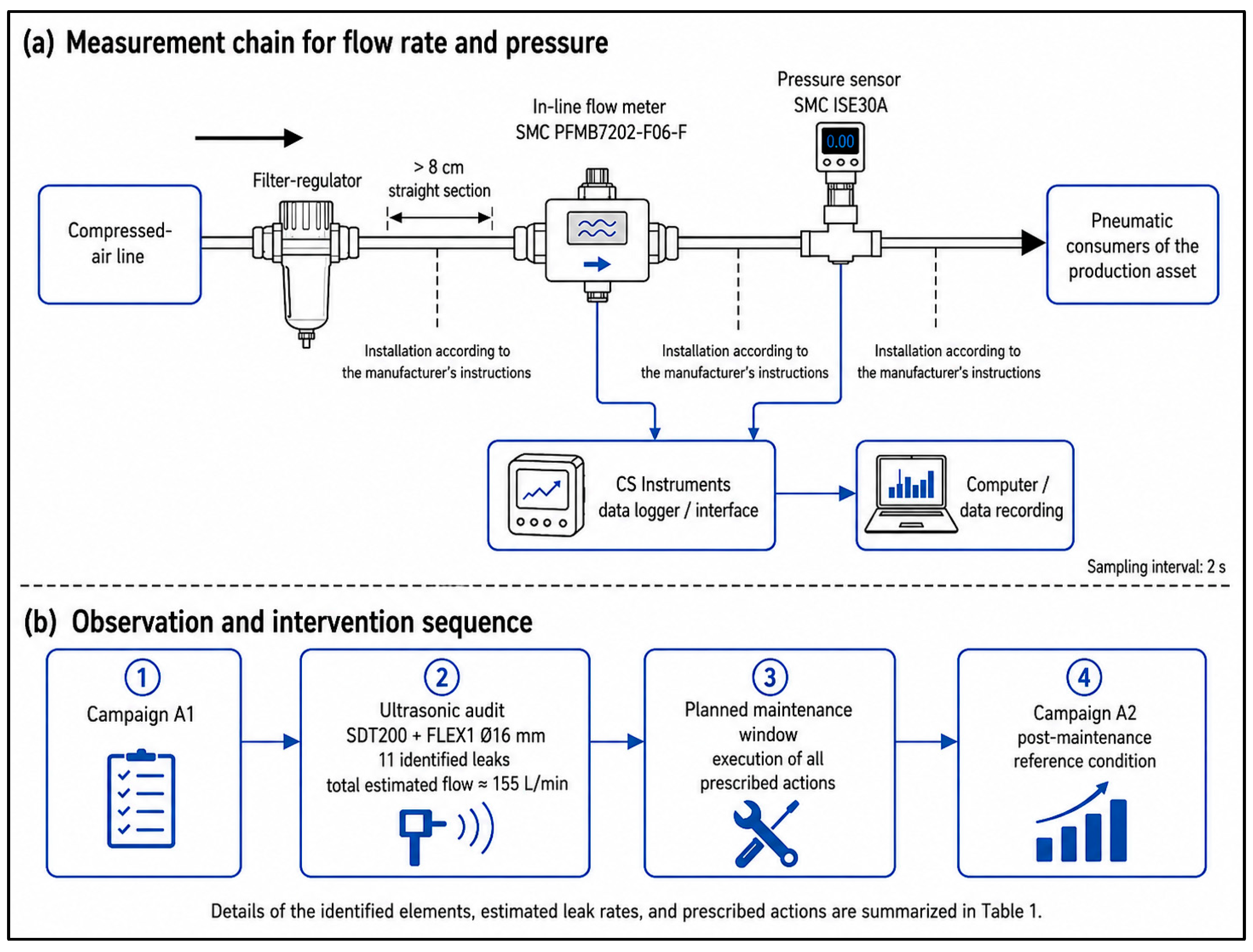
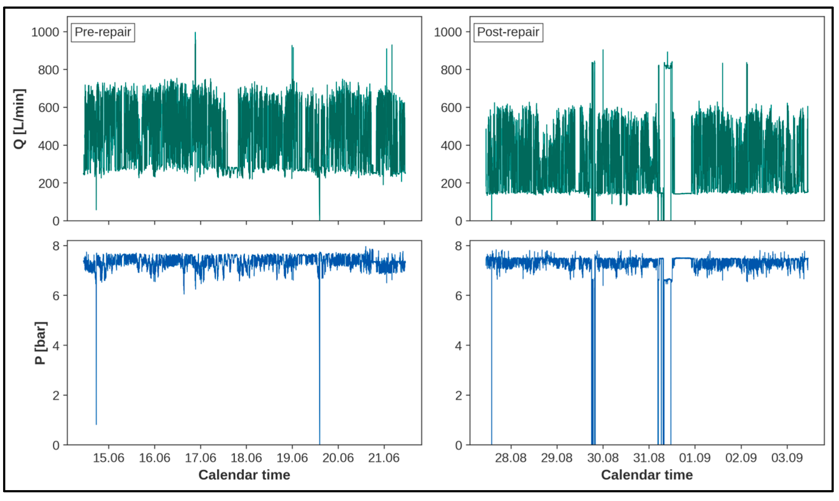
The study was conducted on an operating production machine supplied with compressed air. In both campaigns, flow rate Q [L/min] was measured with the same SMC PFMB7202-F06-F (SMC Co, Tokyo, Japan) thermal flow meter, configured to the Standard reference condition and a 4–20 mA analog output. A filter-regulator was installed between the supply line and the flow meter; the regulating function was not used in the present configuration. Pressure P [bar] was measured with an SMC ISE30A (SMC Co, Tokyo, Japan) mounted perpendicular to the line through a T-fitting. The measurement-chain configuration was unchanged between campaigns. The flow meter was installed in accordance with the manufacturer’s requirements, including a straight section > 8 cm upstream of the sensing element [37], and data were recorded through a CS Instruments logger and interface at 2 s intervals. The pre-repair campaign, A1, ran from 14 to 21 June 2019 and contained 303,266 records. The post-repair campaign, A2, ran from 27 August to 3 September 2019 and contained 302,400 consecutive records, corresponding exactly to 168 h at a 2 s sampling interval. The analysis followed the preserved order of observations. Flow rate and pressure were not interpolated. One-minute medians were used only for visualization in Figure 1. All analytical calculations used the original 2 s data. The measurement-chain schematic and the survey–maintenance–A2 sequence are shown in Figure 2.

No planned change in the production program was made between A1 and A2. This removes one specific alternative explanation for the observed difference, but it does not imply identical actual production load, because short-term technical and process fluctuations remain possible under real operating conditions.

An ultrasonic leak survey was performed immediately after A1 using an SDT200 detector with a FLEX1 resonant sensor, Ø16 mm. The ultrasonic method localizes leakage through the high-frequency acoustic signal generated by turbulent air flow through a defect. Converting the acoustic signal into leak flow is an indirect engineering estimate that depends on leak geometry, pressure, sensor distance and orientation, and the acoustic environment [13,34]. The survey identified 11 leaks with a recorded combined estimate of 155.07 L/min (approximately 155 L/min). This value characterizes the positions identified during the survey and is not treated as an exhaustive measurement of all physically present leaks. The identified positions and prescribed corrective actions are summarized in

Table 1. Ultrasonically identified leaks and prescribed corrective actions. The recorded combined flow estimate for the 11 identified leaks was 155.07 L/min. The values are indirect estimates from the ultrasonic survey rather than direct measurement of the total flow through all physically present leaks.

No.	Component	Estimated Leak Flow [L/min]	Prescription
1	Supply-line fitting (clamp)	14.00	Replace the hose from the main line to the air-preparation unit with pneumatic tubing and pneumatic fittings
2	Supply-line fitting (nipple)	12.62
3	Filter-regulator	10.80	Replace the complete unit
4	Filter-regulator bowl	9.09
5	Valve-island fitting	11.29	Replace
6	Piloted check valve	17.03	Replace
7	Fitting	17.12	Replace
8	Flow-control valve	32.82	Replace
9	Filter-regulator	5.45	Replace
10	Fitting	13.45	Replace
11	Fitting	11.40	Replace
	Total	155.07	—

.

Prescribed corrective actions were implemented during the subsequent planned preventive-maintenance window, approximately three weeks before the start of A2. Because of this interval, A2 is not an immediate post-repair observation. The campaign is used as a stable post-repair reference condition without assuming that the pneumatic system was free of residual or subsequently developed leaks.

Figure 1 shows why weekly averages alone are insufficient for comparison. The flow-rate signal alternates between periods of different production activity, while pressure remains comparatively stable, with several intervals without maintained operating pressure. These intervals are retained in the raw time sequence but do not contribute to the operating-mode or reference-baseline characteristics. The primary analysis therefore compares comparable operating conditions rather than total pre- and post-repair consumption alone.

2.2. Preprocessing and Check for Pressure-Related Effects

The PFMB7202 reading in L/min was used directly as the primary flow-rate signal. No square-root or other pressure-based correction was applied. Before analysis, the input structure and the validity of each sample were checked. A valid sample required numeric values for Q and P and non-negative values for both quantities. Samples with P < 1 bar were treated as conditions without maintained operating pressure but remained valid measurements in the primary time series. The same operating-condition separation rule was applied when Q = 0 and P = 0 simultaneously. A zero Q value at P ≥ 1 bar was retained as a valid observation. The 1 bar threshold served only to distinguish conditions without maintained pressure. It was not a fault criterion, a missing-value rule, or an invalid-record rule. A real operating condition below 1 bar would therefore remain outside the operating-mode analysis.

Pressure was used only to check whether the observed flow difference could be explained by pressure variations. For this check, the linear model in Equation (1) was fitted to valid samples from days 1–5 of the post-repair campaign. Coefficients a and b were estimated by ordinary least squares by minimizing ${\mathsf{\Sigma }}_i{\left[Q_i-\left(a+b{P}_i\right)\right]}^2$. The model was fitted to the paired observations $\left(P_i,Q_i\right)$. For each sample, the residual $r_i$ from Equation (2) quantified the part of the measured flow rate not described by this relationship.

$$Q=a+bP+\epsilon$$

(1)

$$r_i=Q_i-\left(a+b{P}_i\right)$$

(2)

The linear model did not replace the measured flow rate and was not used to set LEADI thresholds. It described only the local relationship between pressure and flow in the post-repair development data and was not interpreted as a physical law or causal model. Its sole purpose was to check whether the primary conclusion remained unchanged after pressure-related variation had been accounted for statistically. Operating-mode segmentation, the reference baseline, LEADI, and the energy assessment all used the flow rate reported by the PFMB7202. This avoided an additional transformation of a quantity that the measurement chain already reports in L/min under the Standard reference condition.

For the additional pre-/post-repair contrast check, the coefficients of the linear relationship were fitted only to samples from the diagnostic operating condition in A2 days 1–5. The same function was then applied unchanged to A1 and A2, after which the median residual was calculated for each of the seven complete 24 h blocks. The pressure-adjusted contrast is the difference between the medians of these daily residuals. Its 95% confidence interval was estimated from 5000 day-level block-bootstrap resamples using PCG64(42). Local linearity and robustness of the result to small changes in P were checked. The model is not treated as a physical law and does not replace directly measured flow rate.

Check for Different Pressurized Exposure Durations

The primary consumed-volume estimate compares A1 and A2 over a common calendar interval of 168 h. A separate check evaluates whether the different durations of intervals without maintained pressure could explain the observed difference. For this sensitivity analysis, the numerator and the denominator are defined over the same set of valid samples with P ≥ 1 bar. For campaign c, pressurized volume is $V_{\mathrm{p}\mathrm{r}\mathrm{e}\mathrm{s}\mathrm{s},c}=\sum \left(Q_i·∆t\right)/\mathrm{60,000}$ using only samples with $P_i\ge 1$ bar, and the corresponding duration is $H_{\mathrm{p}\mathrm{r}\mathrm{e}\mathrm{s}\mathrm{s},c}=N_{\mathrm{p}\mathrm{r}\mathrm{e}\mathrm{s}\mathrm{s},c}·∆t/3600$. Normalized consumption is $r_{\mathrm{p}\mathrm{r}\mathrm{e}\mathrm{s}\mathrm{s},c}=V_{\mathrm{p}\mathrm{r}\mathrm{e}\mathrm{s}\mathrm{s},c}/H_{\mathrm{p}\mathrm{r}\mathrm{e}\mathrm{s}\mathrm{s},c}$, and the relative change is defined as $1-r_{\mathrm{p}\mathrm{r}\mathrm{e}\mathrm{s}\mathrm{s},c},A2/r_{\mathrm{p}\mathrm{r}\mathrm{e}\mathrm{s}\mathrm{s},A1}$.

For a comparable absolute volume, the two normalized rates are projected onto the smaller common pressurized duration, $H_{\mathrm{c}\mathrm{o}\mathrm{m}\mathrm{m}\mathrm{o}\mathrm{n}}=\mathrm{m}\mathrm{i}\mathrm{n}(H_{\mathrm{p}\mathrm{r}\mathrm{e}\mathrm{s}\mathrm{s},A1},H_{\mathrm{p}\mathrm{r}\mathrm{e}\mathrm{s}\mathrm{s},A2})$. Uncertainty in this check is estimated with a day-level block bootstrap, and for each resample volume and pressurized duration are summed over the same selected 24 h blocks. This analysis is a sensitivity check for different pressurized exposure. It does not replace the primary calendar-time comparison and does not control actual production load.

2.3. Operating-Mode Segmentation

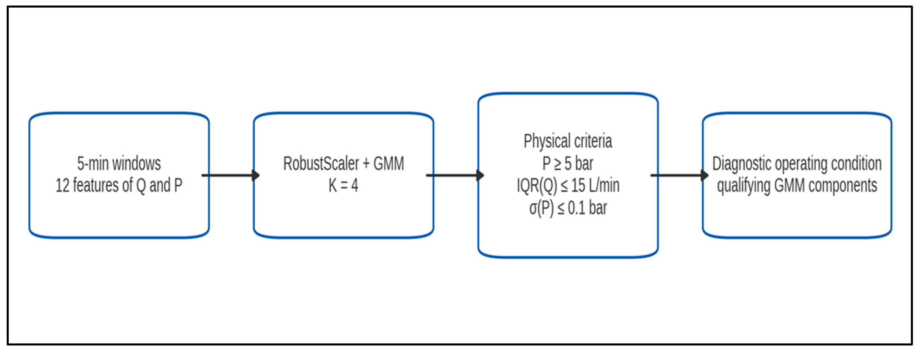
The machine record was divided into non-overlapping 5 min windows, each expected to contain 150 samples. Windows with less than 75% valid samples were excluded from operating-mode clustering. Twelve features were calculated for each remaining window. For flow rate Q, the features were the median, 10th, 25th, 75th, and 90th percentiles, standard deviation, interquartile range (IQR), and mean. For pressure P, the median, standard deviation, and IQR were used. The twelfth feature was the fraction of valid samples under maintained pressure for which $Q>1$ L/min. These features describe the level and within-window variability of flow rate and pressure and were used only by the GMM. Scaling parameters and the GMM were fitted using data reserved for method development (days 1–5 of A1 and A2), without providing the model with the pre-/post-repair label. Days 6–7 were held out for subsequent evaluation. The primary model used $K=4$, a full covariance matrix, $n_{init}=5$, ${\mathrm{m}\mathrm{a}\mathrm{x}}_{\mathrm{i}\mathrm{t}\mathrm{e}\mathrm{r}}=300$, $\mathrm{t}\mathrm{o}\mathrm{l}=0.001$, ${\mathrm{r}\mathrm{e}\mathrm{g}}_{\mathrm{c}\mathrm{o}\mathrm{v}\mathrm{a}\mathrm{r}}={10}^{-6}$, ${\mathrm{i}\mathrm{n}\mathrm{i}\mathrm{t}}_{\mathrm{p}\mathrm{a}\mathrm{r}\mathrm{a}\mathrm{m}\mathrm{s}}=\mathrm{k}\mathrm{m}\mathrm{e}\mathrm{a}\mathrm{n}\mathrm{s}$, and ${\mathrm{r}\mathrm{a}\mathrm{n}\mathrm{d}\mathrm{o}\mathrm{m}}_{\mathrm{s}\mathrm{t}\mathrm{a}\mathrm{t}\mathrm{e}}=42$. The feature vector for one window is denoted by $x_i$.

Before clustering, the features were placed on a comparable scale using RobustScaler: $x^{*}={\displaystyle \frac{x-{\mathrm{m}\mathrm{e}\mathrm{d}}_{\mathrm{t}\mathrm{r}\mathrm{a}\mathrm{i}\mathrm{n}}}{{\mathrm{I}\mathrm{Q}\mathrm{R}}_{\mathrm{t}\mathrm{r}\mathrm{a}\mathrm{i}\mathrm{n}}}}$. The median and IQR were calculated only from development windows. This prevented variables with different units from dominating the model simply because of their numerical scale and reduced the influence of isolated extreme values compared with mean/standard-deviation scaling. The default scikit-learn 1.8.0 settings were used, with centering by the median and scaling by the 25th–75th percentile range. The fitted scaling parameters were then applied unchanged to days 6–7, so the evaluation data could not influence preprocessing.

Equation (3) gives the probability density of the mixture model. The weight ${\pi }_k$ gives the mixture proportion of component k, ${\mu }_k$ is its mean vector, and ${\mathsf{\Sigma }}_k$ is its covariance matrix. GMM does not classify the presence or absence of a fault. It separates recurring groups of 5 min windows with similar flow-rate and pressure characteristics, which can then be interpreted from an engineering perspective.

$$p\left(x_i\right)={\displaystyle {\sum }_{k=1}^K}{\pi }_k\mathcal{N}\left(x_i\mid {\mu }_k,{\mathsf{\Sigma }}_k\right).$$

(3)

The GMM parameters were estimated using the Expectation–Maximization (EM) algorithm. In the E-step, posterior probabilities of component membership were calculated for each window. In the M-step, the component weights, means, and covariance matrices were updated to maximize the likelihood of the observed data. The method assumes that the structure of the scaled 5 min feature vectors can be represented by a finite mixture of multivariate Gaussian components. These components are statistical groups and were not assigned physical operating-mode labels automatically. After fitting, each component was characterized using development data only and checked against the pre-specified, physically motivated selection criteria. All components that met those criteria were combined into one stable low-consumption diagnostic operating condition.

GMM was preferred to k-means because operating modes can differ in variance and in the relationship between flow rate and pressure, and they may overlap during transitions. A full covariance matrix allows each component to have its own geometry in feature space. The primary $K=4$ was pre-specified and was not changed in response to the results. As an additional check on model complexity, the Bayesian Information Criterion (BIC) was calculated as $\mathrm{BIC}=\mathit{p}·\ln \left(n\right)-2·\ln \left(L\right)$, where p is the number of free parameters, n is the number of windows, and L is the maximized likelihood. Lower BIC indicates a better trade-off between fit and complexity, but BIC was not used to choose the primary K. Robustness was assessed separately at $K=3,4,5,\mathrm{and}6$ using unchanged component-selection criteria, with days 6–7 excluded from the selection process.

A GMM component was included in the diagnostic operating condition only if it met all of the following criteria in the development data:

•

At least 5 development windows in the component.

•

Median pressure $P\ge 5\mathrm{b}$ar.

•

Median within-window $IQR\left(Q\right)\le 15\mathrm{L}$/min.

•

Median within-window standard deviation $\sigma \left(P\right)\le 0.1\mathrm{b}$ar.

The absolute median Q is reported but is not used to select components because the change in flow level is the effect that LEADI is intended to measure. If more than one GMM component meets the criteria, all qualifying components are combined into one diagnostic operating condition. A component is not required to occur in both campaigns. Days 6–7 cannot add or remove components or change their interpretation. The five-window minimum limits the influence of rare components, P ≥ 5 bar requires maintained operating pressure, and the IQR(Q) and σ(P) limits enforce low within-window variability.

These values are engineering parameters for the present study and are not proposed as universal thresholds for other machines. Figure 3 summarizes the procedure.

From an engineering perspective, the selected diagnostic operating condition represents a pressurized state with low, stable consumption that resembles standby/idle operation. This is an interpretation, not a machine state independently confirmed by a PLC signal. The formal definition relies only on measured pressure and within-window signal variability. Low absolute flow alone is not sufficient evidence that the machine is in standby.

The $K=3⁤-6$ sensitivity analysis applied the same component-selection criteria without retuning. It therefore tested whether the selected diagnostic operating condition and the main conclusion remained stable as the number of GMM components changed. The results are reported in Section 3.

2.4. LEADI: Definition and Decision Rule

Let $\tilde{Q}\left(w\right)$ denote the median flow rate of valid samples belonging to the diagnostic operating condition within time window w. The primary window length was 60 min. Windows did not overlap and were anchored at the start of each campaign. LEADI was calculated only when a 60 min window contained at least 10 min of valid data from the diagnostic operating condition. Such a window is termed evaluable. The fraction of all time windows that were evaluable was reported separately as diagnostic coverage. $Q_{\mathrm{r}\mathrm{e}\mathrm{f}}$ and ${\mathrm{M}\mathrm{A}\mathrm{D}}_{\mathrm{r}\mathrm{e}\mathrm{f}}$ are, respectively, the median and median absolute deviation of flow rate in the diagnostic operating condition, calculated only from days 1–5 of the post-repair campaign. The two scales ${LEADI}_Q$ and ${LEADI}_Z$ are defined by Equations (4) and (5).

$${\mathrm{LEADI}}_Q\left(w\right)=100{\displaystyle \frac{\tilde{Q}\left(w\right)-Q_{\mathrm{r}\mathrm{e}\mathrm{f}}}{Q_{\mathrm{r}\mathrm{e}\mathrm{f}}}}$$

(4)

$${\mathrm{LEADI}}_Z\left(w\right)={\displaystyle \frac{\tilde{Q}\left(w\right)-Q_{\mathrm{r}\mathrm{e}\mathrm{f}}}{1.4826{\mathrm{M}\mathrm{A}\mathrm{D}}_{\mathrm{r}\mathrm{e}\mathrm{f}}}}.$$

(5)

${\mathrm{L}\mathrm{E}\mathrm{A}\mathrm{D}\mathrm{I}}_Q$ and ${\mathrm{L}\mathrm{E}\mathrm{A}\mathrm{D}\mathrm{I}}_Z$ do not provide independent evidence. Both are derived from the same deviation, $\tilde{Q}\left(w\right)-Q_{\mathrm{r}\mathrm{e}\mathrm{f}}$. The joint requirement ${\mathrm{L}\mathrm{E}\mathrm{A}\mathrm{D}\mathrm{I}}_Q>{\theta }_Q$ and ${\mathrm{L}\mathrm{E}\mathrm{A}\mathrm{D}\mathrm{I}}_Z>{\theta }_Z$ is therefore equivalent to a single threshold on the flow-rate difference. Under the primary setting, ${\theta }_Q=25\%,{\theta }_Z=3$, and the equivalent decision rule is given in Equation (6). ${\mathrm{L}\mathrm{E}\mathrm{A}\mathrm{D}\mathrm{I}}_Q$ expresses the deviation as a percentage of normal consumption. ${\mathrm{L}\mathrm{E}\mathrm{A}\mathrm{D}\mathrm{I}}_Z$ expresses the same deviation relative to the robust dispersion scale $1.4826·{\mathrm{M}\mathrm{A}\mathrm{D}}_{\mathrm{r}\mathrm{e}\mathrm{f}}$. This scale is comparable to a standard deviation when the reference distribution is approximately normal and symmetric. The calculation is defined only when $Q_{\mathrm{r}\mathrm{e}\mathrm{f}}>0,{\mathrm{M}\mathrm{A}\mathrm{D}}_{\mathrm{r}\mathrm{e}\mathrm{f}}>0$, and the diagnostic operating condition must also retain comparable physical meaning in the reference and evaluation periods.

$$\tilde{Q}\left(w\right)-Q_{\mathrm{r}\mathrm{e}\mathrm{f}}>T_{\mathrm{e}\mathrm{f}\mathrm{f}},T_{\mathrm{e}\mathrm{f}\mathrm{f}}=\max \left[{\displaystyle \frac{{\theta }_Q}{100}}·Q_{ref},{\theta }_Z·1.4826·{\mathrm{MAD}}_{\mathrm{ref}}\right]$$

(6)

The procedure generated a maintenance trigger only after three consecutive evaluable windows had been classified as anomalous. A window without enough data for LEADI evaluation broke the sequence. This persistence rule was specified before evaluation and was not selected from the observed results. The primary diagnostic result remained the fraction of anomalous windows among evaluable windows. Days 6–7 of both campaigns were used for the primary evaluation and did not contribute to fitting the GMM, selecting the diagnostic operating condition, or estimating $Q_{\mathrm{r}\mathrm{e}\mathrm{f}}$ or ${\mathrm{MAD}}_{\mathrm{ref}}$. The full campaigns were examined only retrospectively. Threshold sensitivity was assessed at ${\theta }_Q=15,20,25,30\mathrm{and}40\%$ with ${\theta }_Z=3$, and window-length sensitivity was assessed at 30, 60, and 120 min. Diagnostic coverage was reported for every setting.

2.4.1. Simple p05 Comparator Without Operating-Mode Selection

A simple ablation comparator was used to determine how much of the separation between campaigns is already present in the low-flow region of the raw signal without GMM. For each non-overlapping 60 min calendar window, the fifth percentile p05 was calculated from all valid Q measurements. No GMM selection, P ≥ 1 bar condition, or minimum threshold for the fraction of pressurized samples was applied. The reference value ${p05}_{\mathrm{r}\mathrm{e}\mathrm{f}}$ was the median of the hourly p05 values from A2 days 1–5. A window was flagged positive when $p05\left(w\right)>1.25·{p05}_{\mathrm{r}\mathrm{e}\mathrm{f}}$. Days 6–7 remained held out for evaluation. This comparator removes the operating-mode layer from the analytical sequence and is not used to localize or prove a specific leak.

2.4.2. Check of the Fixed Threshold in Development Data

The threshold ${\theta }_Q=25\%$ was fixed before evaluation and was not tuned using days 6–7. As an additional check performed after it had been fixed, the empirical distribution of ${\mathrm{L}\mathrm{E}\mathrm{A}\mathrm{D}\mathrm{I}}_Q$ was examined only in A2 days 1–5 for evaluable windows of 30, 60, and 120 min. The median, 90th percentile, 99th percentile, and maximum were calculated. These quantities indicate how conservative the fixed threshold is relative to the observed post-repair variability in the development period. They are not presented as the procedure by which the threshold was originally selected.

2.4.3. Availability-Limited Decision Latency

The exact interval from physical leak onset to the first LEADI signal cannot be determined because the onset time was not observed. Only the latency caused by the availability of evaluable diagnostic windows is therefore assessed. For successive evaluable windows, the gap between consecutive window starts is calculated, and the median, 90th percentile, and maximum are reported for the full campaigns. With the primary 60 min window and a requirement for three consecutive positive evaluable windows, the theoretical minimum decision time is 3 h under continuous evaluability. A non-evaluable window breaks the sequence and can substantially extend the time to a decision. This measure characterizes the limitation imposed by operating-mode coverage, not the physical detection speed from the moment a defect occurs.

2.4.4. Sensitivity to Minimum Diagnostic Duration and Alarm Persistence

The minimum requirement of 10 min of diagnostic data within a 60 min window directly affects the number of evaluable windows. As a separate post-review sensitivity check, it is varied to 5, 10, 15, and 20 min while the GMM, the selected components, $Q_{\mathrm{r}\mathrm{e}\mathrm{f}}$, ${\mathrm{M}\mathrm{A}\mathrm{D}}_{ref}$, ${\theta }_Q=25\%$, and ${\theta }_Z=3$ remain fixed. For each setting on days 6–7, the number of evaluable windows, the diagnostic coverage, and the number of positive decisions are reported. The tested values are not used to reselect the nominal 10 min setting.

Alarm persistence is checked separately at 2, 3, and 4 consecutive positive evaluable windows. A non-evaluable window breaks the sequence, as in the nominal rule. For each setting, the number of alarm episodes formed in A1 and A2 days 6–7 is reported. The nominal value remains three windows. The check characterizes the trade-off between persistence and the ability to form a signal under incomplete diagnostic coverage and does not constitute tuning to the test results.

2.5. Energy Assessment

The energy assessment starts from the directly measured compressed-air volume and then converts the measured volume difference to scenario-based electricity use. Equations (7) and (8) define the volume integration and the SEC-based energy conversion, respectively.

$$V[{\mathrm{m}}^3]={\displaystyle \frac{1}{\mathrm{60,000}}}·{\mathsf{\Sigma }}_i{Q}_i[\mathrm{L}/\mathrm{m}\mathrm{i}\mathrm{n}]·{\Delta t}_i[\mathrm{s}]$$

(7)

$$E\left[\mathrm{k}\mathrm{W}\mathrm{h}\right]=V\left[{\mathrm{m}}^3\right]·\mathrm{S}\mathrm{E}\mathrm{C}[\mathrm{k}\mathrm{W}\mathrm{h}/{\mathrm{m}}^3]$$

(8)

Consumed volume was obtained by integrating the directly measured non-negative flow rate at the actual sampling step $\Delta t=2\mathrm{s}$, without interpolation. Campaign A1 lasted 168.481 h and A2 lasted 168.000 h, so the primary comparison used a common duration of 168 h. For a campaign with measured volume $V_{meas}$ and duration $T_h$, the standardized volume was calculated as $V_{168}=V_{\mathrm{m}\mathrm{e}\mathrm{a}\mathrm{s}}·{\displaystyle \frac{168}{T_h}}$. For the cumulative plot, both the time axis and cumulative volume of each campaign were scaled by the same factor ${\displaystyle \frac{168}{T_h}}$. This made the final values directly comparable over 168 h without altering instantaneous Q, operating-mode segmentation, or LEADI thresholds.

The measured volume difference is converted to a scenario-based electrical-energy equivalent using the specific energy consumption of the compressor station (SEC, kWh/m³), defined as electrical energy per unit volume of compressed air produced. SEC was not measured for the specific station, and electricity use is therefore not reported as a measured result. The nominal scenario value of 0.153 kWh/m³ corresponds to the mean obtained from measurements and monitoring data from 12 industrial plants, for which individual values ranged from 0.11 to 0.20 kWh/m³ [14]. As independent academic support, Züst et al. report values of approximately 0.11–0.15 kWh/m³ depending on pressure and system configuration [38]. Engineering data from WRS Energie extend this range with specific-consumption examples of 0.12 and 0.16 kWh/m³ for two monitored compressors [39]. Accordingly, 0.153 kWh/m³ is used as an empirically supported nominal scenario, 0.20 kWh/m³ represents the upper end observed in the industrial dataset [14], and 0.10 kWh/m³ is an intentionally conservative lower bound for sensitivity analysis. None of these values is treated as a normative or measured characteristic of the investigated compressor station. The 168 h result is not multiplied to produce an annual value. An annual engineering estimate would require site-specific operating hours, measured SEC, and demonstrated representativeness of the observed effect across the relevant seasons and operating modes.

2.6. Secondary Comparison with Machine-Learning Models

The machine-learning (ML) models are not treated as direct competitors to LEADI because they address a different task. Their role is secondary: to show how statistically separable the observed pre- and post-repair periods are when represented by a common feature set. They do not evaluate the ability to detect future unknown leaks and do not apply the same physical-eligibility rule as LEADI. The primary ML window was 60 min, with 15 min used as a pre-specified window-length sensitivity check. A window entered the ML analysis if it contained at least 75% valid 2 s samples and at least 75% valid 5 min GMM subwindows. Twelve features were used, distinct from the 12 GMM features defined in Section 2.3. Flow rate was represented by its mean, median, standard deviation, 5th percentile (p05), 10th percentile (p10), and 90th percentile (p90). Pressure was represented by its mean and standard deviation. The remaining four features were the fractions assigned to the four K = 4 GMM components. Components 1 and 3 together defined the diagnostic operating condition, but ${\mathrm{L}\mathrm{E}\mathrm{A}\mathrm{D}\mathrm{I}}_Q$, ${\mathrm{L}\mathrm{E}\mathrm{A}\mathrm{D}\mathrm{I}}_Z$, $Q_{\mathrm{r}\mathrm{e}\mathrm{f}}$ and ${\mathrm{M}\mathrm{A}\mathrm{D}}_{\mathrm{r}\mathrm{e}\mathrm{f}}$ were not used as ML inputs. The positive class was the pre-repair state.

2.6.1. Supervised Models

Logistic regression [29] estimated the probability of the pre-repair state as $p\left(y=1|x\right)=\sigma \left({\beta }_0+{\beta }^{T}x\right)$. Because the log-odds are a linear function of the input features, the model served as a simple baseline for testing whether the observed separation required nonlinear relationships. RobustScaler parameters were fitted only on training windows, as in Section 2.3. The settings were $C=1.0$, $\mathrm{s}\mathrm{o}\mathrm{l}\mathrm{v}\mathrm{e}\mathrm{r}\mathrm{=}\mathrm{l}\mathrm{i}\mathrm{b}\mathrm{l}\mathrm{i}\mathrm{n}\mathrm{e}\mathrm{a}\mathrm{r}$, ${\mathrm{c}\mathrm{l}\mathrm{a}\mathrm{s}\mathrm{s}}_{\mathrm{w}\mathrm{e}\mathrm{i}\mathrm{g}\mathrm{h}\mathrm{t}}=\mathrm{b}\mathrm{a}\mathrm{l}\mathrm{a}\mathrm{n}\mathrm{c}\mathrm{e}\mathrm{d}$, ${\mathrm{m}\mathrm{a}\mathrm{x}}_{\mathrm{i}\mathrm{t}\mathrm{e}\mathrm{r}}=2000$, and ${\mathrm{r}\mathrm{a}\mathrm{n}\mathrm{d}\mathrm{o}\mathrm{m}}_{\mathrm{s}\mathrm{t}\mathrm{a}\mathrm{t}\mathrm{e}}=42$. The pre-repair class was selected at $p\ge 0.5$. The main limitation is that the model cannot by itself represent complex nonlinear interactions among the features.

Random Forest [40] combined decision trees trained on bootstrap samples and random subsets of features. The predicted probability was the mean over $B=500$ trees, $p_{RF}\left(x\right)=B^{-1}{\mathsf{\Sigma }}_b{p}_b\left(x\right)$. The ensemble can represent nonlinear relationships and feature interactions, but any resulting separation remains descriptive rather than causal. The settings were $n_{\mathrm{e}\mathrm{s}\mathrm{t}\mathrm{i}\mathrm{m}\mathrm{a}\mathrm{t}\mathrm{o}\mathrm{r}\mathrm{s}}=500$, ${\mathrm{c}\mathrm{l}\mathrm{a}\mathrm{s}\mathrm{s}}_{\mathrm{w}\mathrm{e}\mathrm{i}\mathrm{g}\mathrm{h}\mathrm{t}}=\mathrm{b}\mathrm{a}\mathrm{l}\mathrm{a}\mathrm{n}\mathrm{c}\mathrm{e}\mathrm{d}$, ${max}_{\mathrm{f}\mathrm{e}\mathrm{a}\mathrm{t}\mathrm{u}\mathrm{r}\mathrm{e}\mathrm{s}}=\mathrm{s}\mathrm{q}\mathrm{r}\mathrm{t}$, $\mathrm{b}\mathrm{o}\mathrm{o}\mathrm{t}\mathrm{s}\mathrm{t}\mathrm{r}\mathrm{a}\mathrm{p}\mathrm{=}\mathrm{T}\mathrm{r}\mathrm{u}\mathrm{e}$, and ${\mathrm{r}\mathrm{a}\mathrm{n}\mathrm{d}\mathrm{o}\mathrm{m}}_{\mathrm{s}\mathrm{t}\mathrm{a}\mathrm{t}\mathrm{e}}=42$. All other parameters used the scikit-learn 1.8.0 defaults. The positive-class threshold was 0.5.

Gradient Boosting [41] built a sequence of simple models, each correcting part of the error left by the preceding models. The resulting additive model has the form $F_M\left(x\right)=F_0\left(x\right)+{\mathsf{\Sigma }}_m\eta h_m\left(x\right)$. It provided a second nonlinear supervised comparison. It can represent feature interactions but is sensitive to distributional differences between training and future data. The scikit-learn 1.8.0 defaults were used with ${\mathrm{r}\mathrm{a}\mathrm{n}\mathrm{d}\mathrm{o}\mathrm{m}}_{\mathrm{s}\mathrm{t}\mathrm{a}\mathrm{t}\mathrm{e}}=42$, corresponding to 100 base estimators and ${\mathrm{l}\mathrm{e}\mathrm{a}\mathrm{r}\mathrm{n}\mathrm{i}\mathrm{n}\mathrm{g}}_{\mathrm{r}\mathrm{a}\mathrm{t}\mathrm{e}}=0.1$. Hyperparameters were not tuned in response to test performance. The positive-class threshold was 0.5.

2.6.2. One-Class Anomaly-Detection Models

The one-class models were trained only on post-repair windows designated as normal. Isolation Forest [23] repeatedly partitions feature space at random. An observation that becomes isolated after fewer partitions is treated as more atypical. Its output was converted to an anomaly score $a_{IF}\left(x\right)=-\mathrm{score}\text{\_}\mathrm{samples}\left(x\right)$. The model used 500 trees, $\mathrm{c}\mathrm{o}\mathrm{n}\mathrm{t}\mathrm{a}\mathrm{m}\mathrm{i}\mathrm{n}\mathrm{a}\mathrm{t}\mathrm{i}\mathrm{o}\mathrm{n}\mathrm{=}\mathrm{a}\mathrm{u}\mathrm{t}\mathrm{o}$, and ${\mathrm{r}\mathrm{a}\mathrm{n}\mathrm{d}\mathrm{o}\mathrm{m}}_{\mathrm{s}\mathrm{t}\mathrm{a}\mathrm{t}\mathrm{e}}=42$. One-Class SVM [24] defines a boundary around the region occupied by normal observations in a space induced by an RBF kernel. The parameter $\nu =0.05$ limits the allowed fraction of training observations outside this region, while $\mathrm{g}\mathrm{a}\mathrm{m}\mathrm{m}\mathrm{a}\mathrm{=}\mathrm{s}\mathrm{c}\mathrm{a}\mathrm{l}\mathrm{e}$ determines the kernel scale. Its anomaly score was $a_{\mathrm{O}\mathrm{C}\mathrm{S}\mathrm{V}\mathrm{M}}\left(x\right)=-\mathrm{decision}\text{\_}\mathrm{function}\left(x\right)$. For both models, RobustScaler parameters and the detector itself were fitted on A2 days 1–4. Day 5 was excluded from training because it had been reserved in advance for operating-threshold calibration. The threshold was the 95th percentile of the anomaly score on that calibration day. Test labels were therefore used in neither model fitting nor threshold selection.

2.6.3. Temporal Splitting, Threshold Calibration, and Evaluation Metrics

The supervised models used days 1–5 of A1 and A2 for training and days 6–7 of both campaigns for testing. The one-class models used A2 days 1–4 for training, A2 day 5 only for threshold calibration, and A1 and A2 days 6–7 for testing. The operating-mode GMM and the criteria defining the diagnostic operating condition had already been fixed by the procedure in Section 2.3 and were not changed in response to the ML results. Thus, the statement “trained only on normal data” applies to Isolation Forest and One-Class SVM themselves, not to the preceding operating-mode segmentation.

Model performance was summarized with several complementary metrics. Balanced accuracy $\mathrm{B}\mathrm{A}\mathrm{=}{\displaystyle \frac{\mathrm{T}\mathrm{P}\mathrm{R}\mathrm{+}\mathrm{T}\mathrm{N}\mathrm{R}}{\mathrm{2}}}$ is the mean of the true-positive and true-negative rates and is suitable when the classes are not equally represented. Precision ${\displaystyle \frac{\mathrm{T}\mathrm{P}}{\mathrm{T}\mathrm{P}\mathrm{+}\mathrm{F}\mathrm{P}}}$ is the fraction of positive model decisions that are correct, while sensitivity/recall ${\displaystyle \frac{\mathrm{T}\mathrm{P}}{\mathrm{T}\mathrm{P}\mathrm{+}\mathrm{F}\mathrm{N}}}$ is the fraction of actual positive examples detected. F1 is their harmonic mean. ROC-AUC measures how well the continuous model score ranks pre-repair windows above post-repair windows independently of a specific threshold. Average precision (AP) summarizes the precision–recall relationship. A false-alarm episode was counted when at least three consecutive positive ML windows occurred in the post-repair test data. “Missed hours” is the total duration of pre-repair test windows classified as negative. Random Forest permutation importance was also calculated by randomly shuffling one feature in the test set and measuring the decrease in balanced accuracy, ${\Delta M}_j=M\left(X\right)-M\left(X_{\pi j}\right)$. One hundred permutations were used for each feature with ${\mathrm{r}\mathrm{a}\mathrm{n}\mathrm{d}\mathrm{o}\mathrm{m}}_{\mathrm{s}\mathrm{t}\mathrm{a}\mathrm{t}\mathrm{e}}=42$. When features are strongly correlated, a small or zero decrease does not necessarily imply absence of information because another correlated feature may substitute for it.

The operating threshold of a one-class model may depend on which normal day is used for calibration. This dependence was examined for the primary 60 min window by rotating the calibration day across the five available A2 days, with each day $d\in \{1,2,3,4,5\}$ of A2 serving once as the calibration day. In each rotation, RobustScaler and the one-class detector were trained on the other four normal days, and the selected day defined the 95th percentile of the anomaly score. The test set on A1 and A2 days 6–7 remained unchanged. For each model, the median, minimum, and maximum balanced accuracy were reported. This sensitivity analysis did not replace the pre-specified primary protocol using calibration day 5 and was not used to select a more favorable threshold after inspection of the test results.

2.7. Metrological Limitations, Statistical Uncertainty, Data-Leakage Prevention, and Reproducibility

The manufacturer-specified accuracy of the measurement chain, the observed variability of the process signal, and the statistical uncertainty of the pre-/post-repair estimate are treated as different quantities. For the PFMB7202-F06-F, the manufacturer specifies ±3% FS for the display and analog output under nominal conditions [37]. Over the nominal 20–2000 L/min range, this corresponds to an absolute catalog limit of ±60 L/min on the indicated level. This limit is not a ±60 L/min uncertainty of the A1–A2 difference, nor is it a standard uncertainty obtained from traceable calibration. Applied only as an absolute indication bound, Q_ref = 144.293 L/min corresponds to 84.293–204.293 L/min. This is not a confidence interval or calibration uncertainty. Because the manufacturer does not specify a between-campaign drift model, the catalog limit is not decomposed into additive and multiplicative terms. Instead, let δ denote an unknown differential shift between A1 and A2. The observed contrasts then become 122.0 − δ L/min and 1370.8 − 10.08δ m³ over 168 h. For |δ| = 60 L/min, the corresponding deterministic sensitivity ranges are 62.0–182.0 L/min and 766.0–1975.6 m³. These ranges are sensitivity bounds, not metrological confidence intervals. The ISE30A is used as a pressure-control variable, and its catalog specifications are used only to define the interpretive limit for observed differences in P [42].

For interpretation of the pre-/post-repair difference, the measurement result can be represented conceptually as ${\tilde{Q}}_c=\left(1+{\epsilon }_g\right)Q_c+b+d_c+{\eta }_c$, where ${\epsilon }_g$ is a common multiplicative conversion-factor error, b is a common additive offset, $d_c$ is campaign-specific drift, and ${\eta }_c$ is a short-term random component. With the same unchanged measurement chain, the common additive offset cancels in the absolute difference, while the common multiplicative error scales both levels and their absolute difference in the same way. Between-campaign drift, however, cannot be determined without a traceable calibration history. Neither independence of systematic errors between A1 and A2 nor complete cancelation of those errors is therefore assumed.

${\mathrm{M}\mathrm{A}\mathrm{D}}_{\mathrm{r}\mathrm{e}\mathrm{f}}$ and the robust scale ${1.4826·\mathrm{M}\mathrm{A}\mathrm{D}}_{\mathrm{r}\mathrm{e}\mathrm{f}}$ characterize the observed short-term variability of the reference process signal, not the metrological accuracy of the flow meter. Likewise, the block bootstrap assesses the sensitivity of the pre-/post-repair difference statistics to the observed 24 h blocks and does not constitute a measurement-uncertainty budget.

The number of 2 s samples was not treated as the number of independent repetitions. Uncertainty in the primary flow-rate difference and the 168 h volume difference was assessed with a day-level block bootstrap. In each of 5000 resamples, complete 24 h blocks were sampled with replacement from the seven complete days in each campaign. The two campaigns were resampled independently using numpy.random.Generator(numpy.random.PCG64(42)), and the 95% confidence interval was defined by the 2.5th and 97.5th percentiles. The resamples therefore show how sensitive the estimate is to the observed days without increasing the number of independent experimental units.

A separate day-level block bootstrap was used for balanced accuracy, ROC-AUC, and average precision (AP). The two A1 test days and two A2 test days were resampled with replacement within their respective classes, with all windows from a selected day kept together. The resulting intervals were used as a robustness check rather than as precise estimates for a broader population, because only two distinct test days were available for each class.

All parameters derived from the data, including scaling, reference baselines, model parameters, and operating thresholds, were estimated only from the pre-specified training or calibration blocks. The canonical public implementation uses Python 3.13.5, NumPy 2.3.5, pandas 2.2.3, SciPy 1.17.0, and scikit-learn 1.8.0 for computation. Matplotlib 3.10.8 and openpyxl 3.1.5 are used for visualization and input/output operations, respectively. Stochastic operations use fixed generators or ${random}_{state}=42$ according to the algorithm. The public code checks the SHA-256 hashes of both input CSV files before analysis and terminates on mismatch. After the test results had been obtained, no thresholds, window lengths, feature sets, or hyperparameters were changed to improve the reported metrics.

3. Results

3.1. Selection of the Diagnostic Operating Condition and Change in Baseline Flow

The structural check found no invalid primary records: 0/303,266 in A1 and 0/302,400 in A2. Samples at P < 1 bar are valid measurements rather than missing or corrupted data. They comprise 257 samples (0.143 h) in A1 and 3505 samples (1.947 h) in A2. With 5 min operating-mode clustering, 2020 of 2022 windows in A1 and 1986 of 2016 in A2 met the minimum requirement of 75% valid samples. The remaining windows were not passed to the GMM and were not interpreted as a separate machine operating mode.

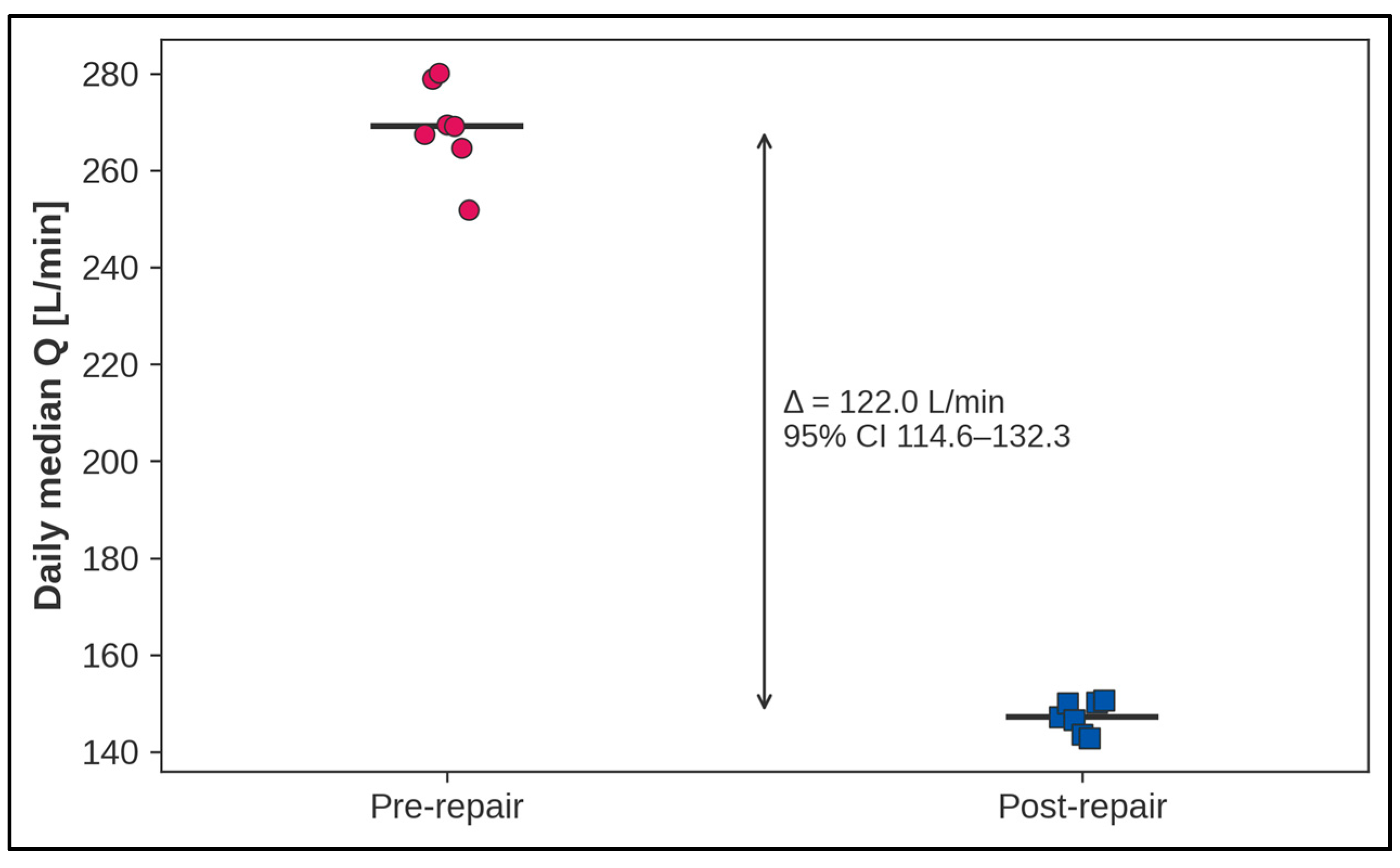
With the primary K = 4, two GMM components, 1 and 3, met the pre-specified physical criteria and together formed the diagnostic operating condition. For component 1, the median Q in the development days was 143.7 L/min, the median IQR(Q) was 3.21 L/min, and the median σ(P) was 0.0148 bar. The corresponding values for component 3 were 269.9 L/min, 3.66 L/min, and 0.0147 bar. The two components had similarly low within-window variability and maintained pressure but different absolute flow levels. This supports the decision not to use Q itself as a criterion for defining the condition. The two components did not co-occur within a campaign: component 3 accounted for all 229 diagnostic-condition windows in the development subset and 312 such windows in the full A1 campaign, whereas component 1 accounted for the corresponding 260 and 345 windows in A2. No evaluable 60 min window contained both components, and the reference baseline was derived entirely from component 1. Across the full campaigns, the median 5 min flow rate in the diagnostic operating condition was 266.7 L/min before maintenance and 145.5 L/min after maintenance. Treating each complete day as one block gave an estimated difference of 122.0 L/min with a 95% CI of 114.6–132.3 L/min. On the same day-level basis, the relative reduction was 45.3% (95% CI 43.3–47.4%). The observed change is consistent with reduced parasitic demand after the technical intervention, but the before/after design does not allow the entire difference to be attributed causally to the repaired positions alone.

The ultrasonic estimate, which is independent in measurement principle, provides additional physical context for the scale of the change. The 11 leaks identified immediately after A1 had a combined estimated flow of approximately 155 L/min. This aggregated acoustic estimate and the 122.0 L/min difference estimated from daily blocks are not the same measured quantity and are not used for numerical validation. Their agreement in direction and order of magnitude provides additional physical support for interpreting the observed change as associated with the maintenance intervention. The daily block-level values underlying this estimate are shown in Figure 4. The difference between the two values cannot be used to calculate the flow of residual or newly developed leaks.

Figure 4. Daily medians of directly measured flow rate Q [L/min] in the stable low-consumption diagnostic operating condition for the seven complete 24 h blocks before and after repair. Horizontal lines show the medians of the daily values. The difference is 122.0 L/min, and the 95% CI of 114.6–132.3 L/min was obtained by a block bootstrap with 5000 resamples.

Figure 4. Daily medians of directly measured flow rate Q [L/min] in the stable low-consumption diagnostic operating condition for the seven complete 24 h blocks before and after repair. Horizontal lines show the medians of the daily values. The difference is 122.0 L/min, and the 95% CI of 114.6–132.3 L/min was obtained by a block bootstrap with 5000 resamples.

Mean pressure over valid samples was 7.2903 bar before maintenance and 7.2736 bar after maintenance, a difference of 0.0167 bar. This difference is smaller than the absolute catalog accuracy of the ISE30A [42] and does not justify concluding that the true mean pressure was exactly identical. Within the diagnostic operating condition, the linear model fitted only to A2 days 1–5 was $Q=31.347+15.268·P$ with R² = 0.021. The local linear relationship with P therefore explained approximately 2.1% of the variation in Q in this development set, and the value does not establish the absence of nonlinear or operating-mode effects. After subtracting this relationship, the difference between the daily median residuals was 120.05 L/min with a 95% day-level block-bootstrap CI of 112.30–130.12 L/min. Its proximity to the primary estimate of 122.03 L/min (95% CI 114.63–132.27) shows that the small observed pressure difference does not explain the primary contrast. This remains a sensitivity analysis rather than a correction of the main LEADI result.

The pre-specified K = 4 was retained. Robustness was assessed separately. For K = 3, 4, 5, and 6, the positive/evaluable A1 windows were 20/20, 19/19, 19/19, and 18/18, respectively, whereas A2 gave 0/17, 0/17, 0/17, and 0/16. BIC decreased monotonically over the tested range, from −115,408.9 at K = 3 to −116,520.1 at K = 4, −121,552.0 at K = 5, and −122,411.0 at K = 6, so K = 4 was not the BIC optimum within this limited set of values. Because the main conclusion was preserved at K = 3–6, BIC is used only as a diagnostic measure of model complexity, not for retrospective selection of a more favorable K.

The change in total consumed volume was of the same order as the change in baseline flow. Over an equal duration of 168 h, measured volume was 4743.8 m³ before repair and 3373.0 m³ after repair, a difference of 1370.8 m³. Total volume also includes active production modes, so the difference between this value and the estimate from the diagnostic operating condition cannot be used to allocate the loss quantitatively among individual leaks.

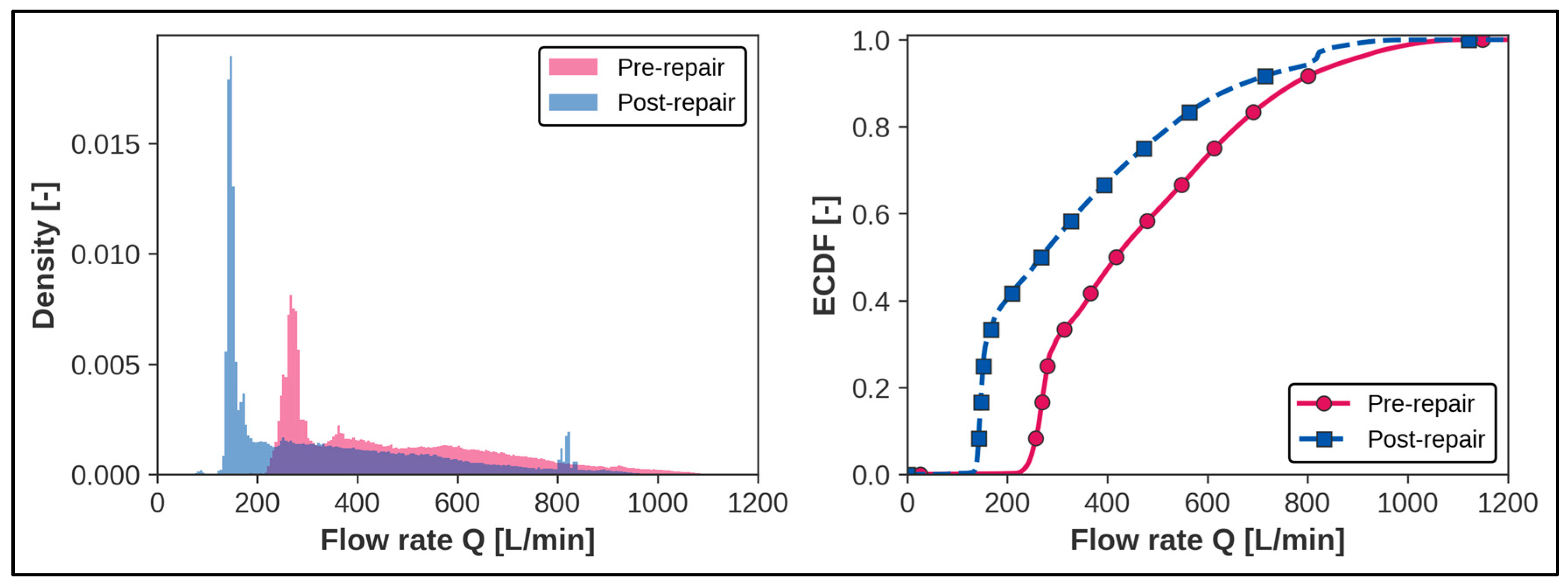
The distribution of all valid measurements provides additional context for the observed change. Figure 5 shows that the largest shift between campaigns occurs in the low-flow region, where useful pneumatic demand is most limited. The Figure 5 is descriptive. The primary conclusion is based on the comparison within the pre-specified diagnostic operating condition.

3.2. LEADI Results and Robustness

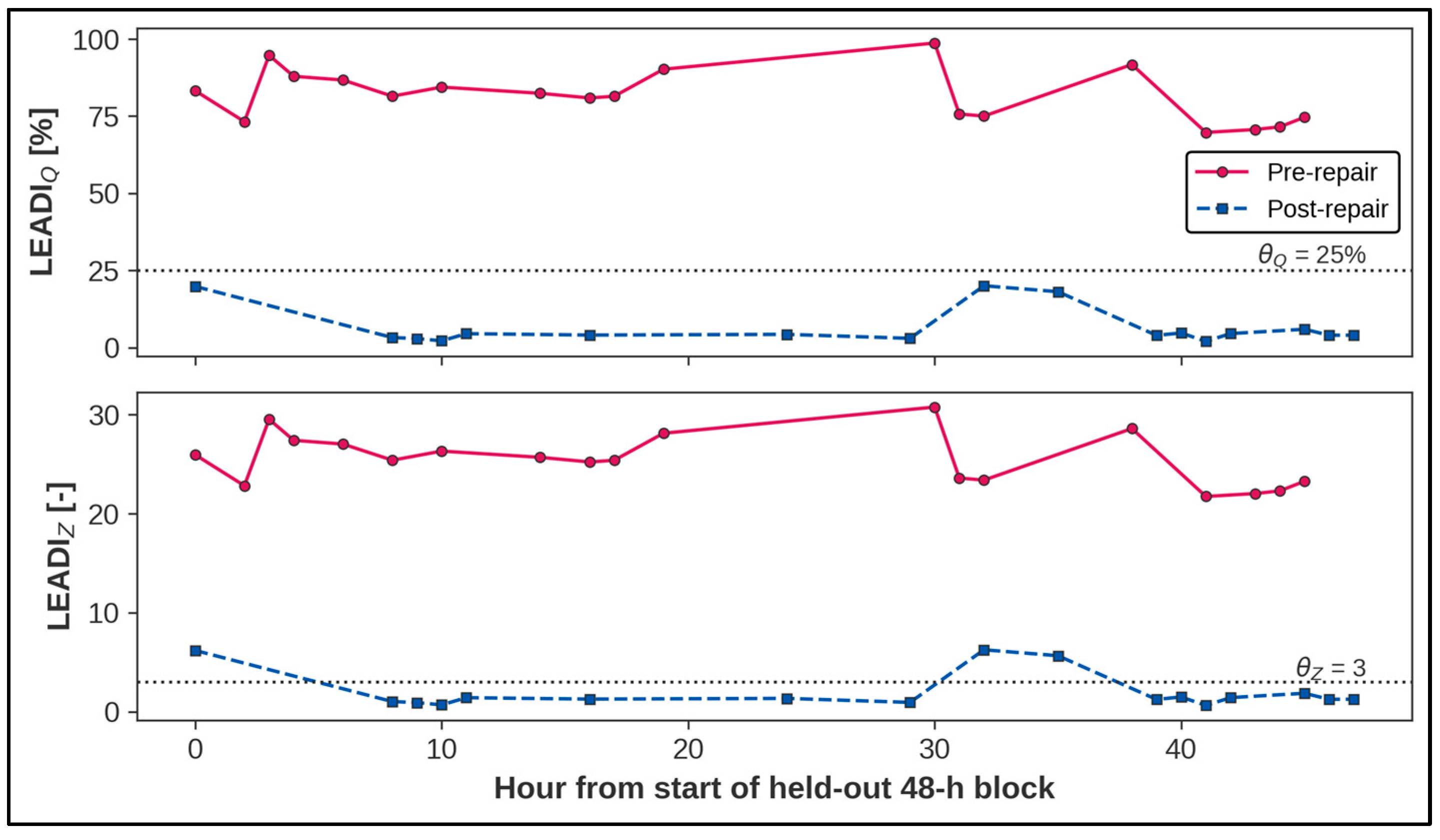
Figure 6 shows the two LEADI scales for evaluable 60 min windows on days 6–7. Windows without at least 10 min of data from the diagnostic operating condition are not plotted as normal values and remain without a decision. ${\mathrm{L}\mathrm{E}\mathrm{A}\mathrm{D}\mathrm{I}}_Q$ and ${\mathrm{L}\mathrm{E}\mathrm{A}\mathrm{D}\mathrm{I}}_Z$ measure the same deviation in different units. With $Q_{\mathrm{r}\mathrm{e}\mathrm{f}}=144.293$ L/min and ${\mathrm{M}\mathrm{A}\mathrm{D}}_{\mathrm{r}\mathrm{e}\mathrm{f}}=3.122$ L/min, ${\theta }_Q=25\%$ requires a flow increase of 36.073 L/min, whereas ${\theta }_Z=3$ corresponds to 13.886 L/min. Under the primary setting, the decision is therefore governed by the stricter relative threshold ${\theta }_Q$.

On days 6–7, all 19 evaluable pre-repair windows exceeded the decision threshold, whereas none of the 17 evaluable post-repair windows was flagged as anomalous. Median ${\mathrm{L}\mathrm{E}\mathrm{A}\mathrm{D}\mathrm{I}}_Q$ was 81.5% before repair and 4.0% after repair. Requiring three consecutive anomalous evaluable windows produced three alarm episodes before repair and none after repair. This episode-level result is secondary to the window-level result because any window without sufficient data from the diagnostic operating condition breaks the sequence.

The reference baseline, calculated only from A2 days 1–5, was $Q_{\mathrm{r}\mathrm{e}\mathrm{f}}=144.293$ L/min and ${\mathrm{M}\mathrm{A}\mathrm{D}}_{\mathrm{r}\mathrm{e}\mathrm{f}}=3.122$ L/min. The robust scale ${1.4826·\mathrm{M}\mathrm{A}\mathrm{D}}_{\mathrm{r}\mathrm{e}\mathrm{f}}$ is approximately 4.63 L/min and describes the observed short-term variability of the reference process signal, not the accuracy of the flow meter. With 60 min windows, diagnostic coverage on days 6–7 was 39.6% before maintenance and 35.4% after maintenance. Retrospective analysis of the full campaigns gave coverage of 37.3% and 33.9%. At the primary threshold, all 63 evaluable pre-repair windows were anomalous and none of the 57 evaluable post-repair windows was anomalous. Complete separation therefore applies only to windows containing sufficient data from the diagnostic operating condition and should not be interpreted as universal sensitivity and specificity.

The p05 ablation comparator used ${p05}_{\mathrm{r}\mathrm{e}\mathrm{f}}=143.311\mathrm{L}$/min and a threshold of 179.139 L/min. On held-out days 6–7, it flagged 47/48 pre-repair and 1/48 post-repair hourly windows. Across the full campaigns, the result was 167/169 versus 9/168, and the final incomplete hourly window of A1 was retained in the retrospective count. The fifth percentile of flow rate therefore almost separates the two observed campaigns even without GMM. The operating-mode layer of LEADI does not increase discriminative performance. Its function is to restrict decisions to a pre-specified physically eligible condition and to expose, through diagnostic coverage, the limitation imposed by that selectivity.

The additional check of the fixed threshold on A2 days 1–5 shows that, for the primary 60 min windows, ${\mathrm{L}\mathrm{E}\mathrm{A}\mathrm{D}\mathrm{I}}_Q$ has a median of 0.09%, a 90th percentile of 5.65%, a 99th percentile of 7.96%, and a maximum of 7.98%. At 30 and 120 min, the maximum values are 8.34% and 7.53%, respectively. All are well below ${\theta }_Q=25\%$. This comparison shows that the fixed threshold is conservative relative to the observed post-repair variability in the development data without using days 6–7 for threshold tuning.

Table 2. Sensitivity of the LEADI result to ${\theta }_Q$ on days 6–7 using 60 min windows and ${\theta }_Z=3$. Percentages are calculated only over windows containing at least 10 min of valid data from the diagnostic operating condition and therefore eligible for LEADI evaluation. There were 19 such windows before maintenance and 17 after maintenance.

Threshold ${\mathit{\theta }}_{\mathit{Q}}$	Anomalous Pre-Repair Windows	Anomalous Post-Repair Windows
15%	100% (19/19)	17.6% (3/17)
20%	100% (19/19)	5.9% (1/17)
25% (primary)	100% (19/19)	0% (0/17)
30%	100% (19/19)	0% (0/17)
40%	100% (19/19)	0% (0/17)

shows threshold sensitivity on days 6–7 using 60 min windows. Complete separation is retained at ${\theta }_Q=25-40\%$. At 20%, one of the 17 post-repair windows is flagged as anomalous, and at 15%, three are flagged. Window length mainly affects diagnostic coverage. At the primary threshold, all evaluable pre-repair windows and no evaluable post-repair windows are anomalous at 30, 60, and 120 min. Coverage is 19.8%/20.8%, 39.6%/35.4%, and 62.5%/54.2% before/after maintenance, respectively. A longer window increases the probability of containing sufficient data from the diagnostic operating condition but reduces temporal resolution. The exact leak onset was not observed, so the physical delay from onset to first signal cannot be estimated.

Changing the minimum diagnostic duration alters coverage but does not change separation among evaluable windows. At 5, 10, 15, and 20 min, the positive/evaluable A1 windows are 25/25, 19/19, 11/11, and 7/7, respectively, while A2 remains 0/23, 0/17, 0/14, and 0/10. Diagnostic coverage is 52.1%, 39.6%, 22.9%, and 14.6% in A1 and 47.9%, 35.4%, 29.2%, and 20.8% in A2. Under the stricter 15- and 20 min requirements, coverage is higher in A2, indicating greater availability of the selected diagnostic operating condition within 60 min windows after maintenance. This is a descriptive result and is not used for causal interpretation. Minimum diagnostic duration primarily controls decision availability rather than the direction of separation in the observed dataset.

With the nominal 10 min requirement, the persistence condition forms 4/0 alarm episodes in A1/A2 with two consecutive positive windows, 3/0 with three, and 0/0 with four. Four consecutive windows are too strict for the observed intermittent operating-mode coverage because no alarm forms even in A1. The nominal three-window rule retains a signal in A1 without producing an alarm episode in A2. This check shows the influence of the parameter and is not used to optimize the nominal value retrospectively.

Across the full campaigns, the median interval between the starts of successive evaluable 60 min windows is 2 h in both A1 and A2. The 90th percentile is 5.8 h for A1 and 6.5 h for A2, and the maximum observed interval is 13 h and 8 h, respectively. With a persistence requirement of three windows, the theoretical minimum decision time is 3 h only when three consecutive hourly windows are evaluable. The observed intervals show that operating-mode coverage can extend decision time substantially beyond this minimum. This is availability-limited latency, not a measured delay from physical leak onset.

3.3. Energy Impact

The directly integrated volume was 4757.4 m³ over 168.481 h in A1 and 3373.0 m³ over 168.000 h in A2. After scaling to a common calendar basis of 168 h, pre-repair volume was 4743.8 m³. The difference was 1370.8 m³, or 28.90%. A day-level block bootstrap gave a point estimate of 1375.7 m³ and a 95% CI of 1064.7–1678.4 m³ using a fixed PCG64(42) generator and 5000 resamples. The interval characterizes variation in the estimate across the observed daily blocks and does not represent metrological uncertainty of the flow meter.

In A1, valid time at P ≥ 1 bar was 168.338 h, compared with 166.053 h in A2. Volume integrated only over those same pressurized samples was 4757.267 and 3372.970 m³, respectively, corresponding to 28.260 and 20.313 m³ per pressurized hour. The relative reduction was 28.12%, with a 95% day-level block-bootstrap interval of 22.16–33.57%. To retain the same definition of numerator and denominator, the comparable absolute-volume difference is obtained from the difference between the two rates normalized only over samples at P ≥ 1 bar and projected onto the common pressurized duration of 166.053 h. The resulting difference is 1319.7 m³ (95% CI 998.0–1638.7 m³), and the calendar volume of A2 is not used in this calculation. Volume integrated at P < 1 bar was only 0.105 m³ in A1 and 0.024 m³ in A2. The different depressurized durations therefore do not explain the primary calendar-time reduction of 28.90%, although this check does not control other operational differences.

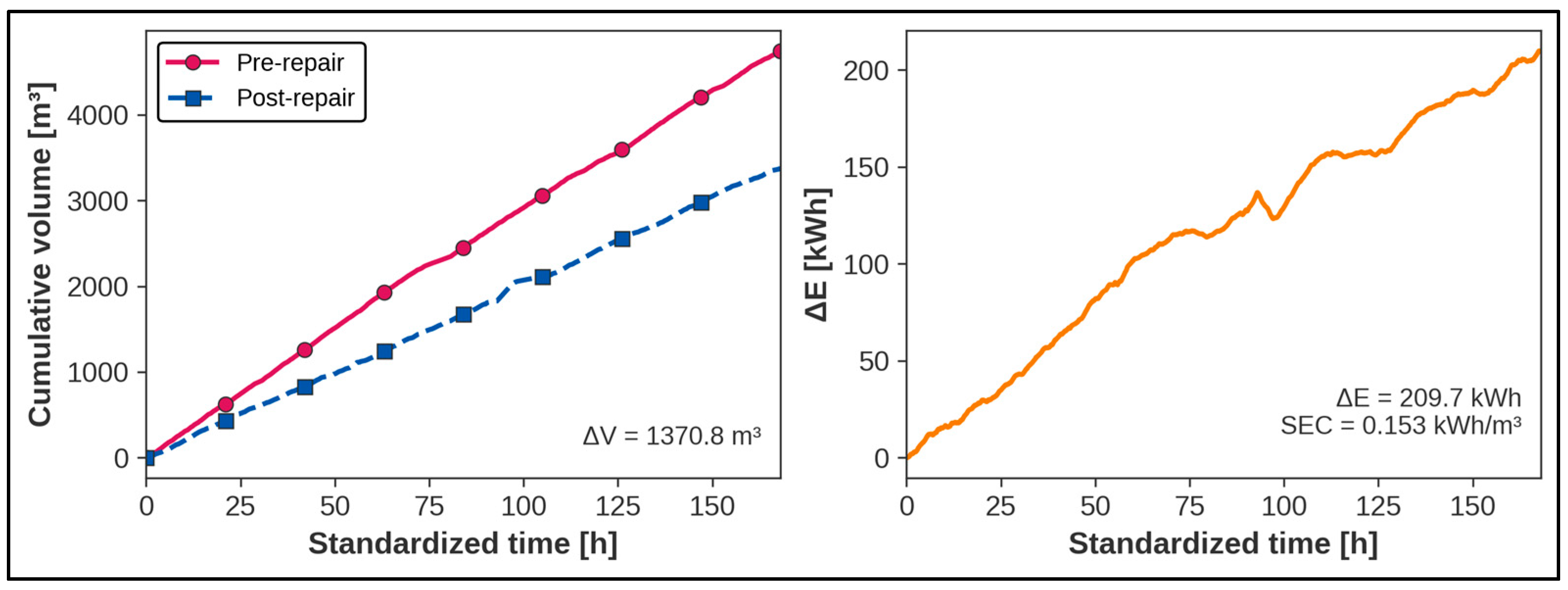
For the measured calendar-time difference ΔV = 1370.8 m³, the scenario-based electrical-energy equivalent over the same 168 h is 137.1 kWh at SEC = 0.10 kWh/m³, 209.7 kWh at 0.153 kWh/m³, and 274.2 kWh at 0.20 kWh/m³. All three values are calculated scenarios rather than measured electrical energy, and they are not extrapolated to an annual figure.

Table 3. Scenario-based electrical-energy equivalent for a measured volume difference of 1370.8 m³ over a common 168 h basis and three values of compressor-station specific energy consumption (SEC). The values are calculated scenarios and do not represent directly measured electrical energy.

SEC [kWh/m3]	ΔE over 168 h [kWh]
0.10	137.1
0.153 (nominal scenario)	209.7
0.20	274.2

summarizes the three scenarios. Figure 7 shows how the volume difference and the corresponding energy scenario accumulated over 168 h.

The cumulative curves show that the difference did not arise from a single short episode. Instead, it accumulated throughout the observation period, consistent with persistently lower compressed-air consumption after repair. The shape of the curves alone does not identify the cause of the change.

3.4. Comparison with Machine-Learning Models

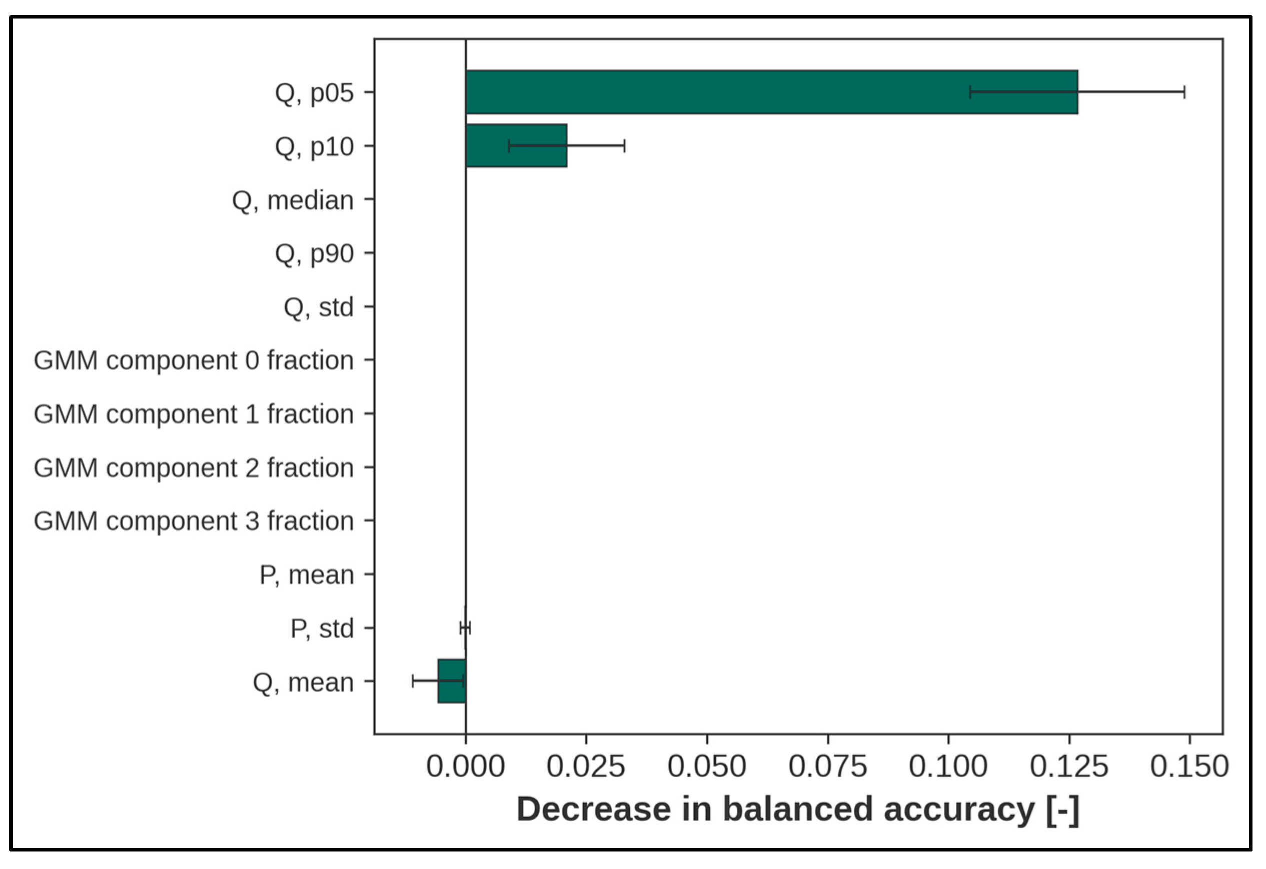
Table 4 summarizes the secondary machine-learning comparison under the pre-specified temporal split and 60 min windows. The supervised models use 236 training windows and 96 test windows. The one-class models use 92 normal A2 windows for training, 24 separate A2 windows for threshold calibration, and the same 96 test windows. These results show how statistically separable the two observed periods are, not whether the models will detect a future unknown leak. Figure 8 presents Random Forest permutation importance.

Table 4. Secondary comparison of models for separating the observed pre- and post-repair states using 60 min windows. Days 6–7 were the test period for all models. Average precision (AP) summarizes the precision–recall relationship. A false-alarm episode was counted when at least three consecutive positive post-repair windows occurred. “Missed hours” is the total duration of pre-repair test windows with false-negative decisions. Eligibility for the machine-learning analysis differs from eligibility for LEADI calculation, so A1 contains 48 test windows whereas LEADI could be evaluated for 19 windows over the same days 6–7. See Table 5 for the dependence of one-class results on the calibration day.

Model	Balanced Accuracy	ROC-AUC	Average Precision (AP)	False-Alarm Episodes/Day	Missed Hours
Logistic Regression	0.885	0.991	0.991	0.00	11
Random Forest	0.979	1.000	1.000	0.00	2
Gradient Boosting	0.990	1.000	1.000	0.00	1
Isolation Forest	0.500	0.951	0.902	0.00	48
One-Class SVM	0.990	1.000	1.000	0.00	1

Table 4. Secondary comparison of models for separating the observed pre- and post-repair states using 60 min windows. Days 6–7 were the test period for all models. Average precision (AP) summarizes the precision–recall relationship. A false-alarm episode was counted when at least three consecutive positive post-repair windows occurred. “Missed hours” is the total duration of pre-repair test windows with false-negative decisions. Eligibility for the machine-learning analysis differs from eligibility for LEADI calculation, so A1 contains 48 test windows whereas LEADI could be evaluated for 19 windows over the same days 6–7. See Table 5 for the dependence of one-class results on the calibration day.

Model	Balanced Accuracy	ROC-AUC	Average Precision (AP)	False-Alarm Episodes/Day	Missed Hours
Logistic Regression	0.885	0.991	0.991	0.00	11
Random Forest	0.979	1.000	1.000	0.00	2
Gradient Boosting	0.990	1.000	1.000	0.00	1
Isolation Forest	0.500	0.951	0.902	0.00	48
One-Class SVM	0.990	1.000	1.000	0.00	1

Table 5. Sensitivity of one-class model performance to the choice of calibration day using 60 min windows. The primary analysis used A2 days 1–4 for training and A2 day 5 to set the 95th percentile of the anomaly score. In the sensitivity analysis, each of A2 days 1–5 was used in turn for calibration and the other four days for training. The test set, A1 and A2 days 6–7, remained unchanged and was not used to select the calibration day.

Model	Primary Balanced Accuracy (A2 Day 5)	Balanced Accuracy Under Calibration-Day Rotation Median [Min–Max]
Isolation Forest	0.500	0.531 [0.500–0.854]
One-Class SVM	0.990	0.958 [0.656–0.990]

Table 5. Sensitivity of one-class model performance to the choice of calibration day using 60 min windows. The primary analysis used A2 days 1–4 for training and A2 day 5 to set the 95th percentile of the anomaly score. In the sensitivity analysis, each of A2 days 1–5 was used in turn for calibration and the other four days for training. The test set, A1 and A2 days 6–7, remained unchanged and was not used to select the calibration day.

Model	Primary Balanced Accuracy (A2 Day 5)	Balanced Accuracy Under Calibration-Day Rotation Median [Min–Max]
Isolation Forest	0.500	0.531 [0.500–0.854]
One-Class SVM	0.990	0.958 [0.656–0.990]

The permutation check shows that Random Forest relies most clearly on the lower percentiles of flow rate. Permuting p05 reduced balanced accuracy by 0.126 ± 0.023 on average, while permuting p10 reduced it by 0.021 ± 0.012. For the remaining features, the mean change was zero or close to zero in this test. This does not mean that they contain no information, because several features are strongly correlated and can substitute for one another. The dominant role of p05 is consistent with the ablation comparator, which almost separates the campaigns without GMM. The high separability of the two periods is therefore not used as evidence that operating-mode segmentation by itself increases classification accuracy.

Random Forest achieved a balanced accuracy of 0.979 and a ROC-AUC of 1.000, while Gradient Boosting achieved 0.990 and 1.000, respectively. One-Class SVM also reached 0.990 and 1.000 with 60 min windows, but its balanced accuracy fell to 0.859 with 15 min windows. Isolation Forest illustrates why threshold calibration matters. Its ROC-AUC was 0.951 and AP was 0.902, so the continuous anomaly score ranked the two periods well. At the pre-specified operating threshold, however, balanced accuracy was 0.500 and no pre-repair test window was detected, corresponding to 48 missed hours. The day-level block bootstrap gave a 95% CI of 0.894–1.000 for ROC-AUC, while balanced accuracy remained 0.500–0.500. Strong ranking performance therefore did not translate into a useful binary decision at the selected threshold, and the threshold was not changed after the test results were observed. The One-Class SVM result obtained with calibration day 5 reproduced exactly under the fixed protocol, but the five-day sensitivity analysis showed that it depended on which normal day was used for calibration. Balanced accuracy had a median of 0.958 and a range of 0.656–0.990 for One-Class SVM, and a median of 0.531 with a range of 0.500–0.854 for Isolation Forest. A single point estimate from a one-class model should therefore be interpreted together with its threshold-calibration procedure.

4. Discussion

Interpretation of the results is constrained by four conditions. The study examines one production asset and one repair cycle. The reference baseline is local and post-repair. The diagnostic operating condition is not independently confirmed by a PLC state. And LEADI provides a decision only when the pre-specified operating condition is available. The results therefore constitute a temporally held-out internal evaluation against a local reference baseline, not external validation of a universal leak detector.

The primary result must be interpreted through both separation and diagnostic coverage. Under the primary setting, LEADI flags all evaluable pre-repair windows and no evaluable post-repair windows, and the same direction is retained at K = 3–6 and window lengths of 30–120 min. The simple p05 comparator, however, reaches 47/48 versus 1/48 on held-out days 6–7 without operating-mode selection. The low-flow region therefore carries the main information for separating the two campaigns. The operating-mode layer of LEADI serves a different purpose: it determines when low consumption is physically eligible for engineering comparison and quantifies the cost of this selectivity through diagnostic coverage.

The physical scale of the change is supported by the independent chronology of the leak survey and maintenance intervention. The ultrasonic survey immediately after A1 identified 11 leaks with a combined estimated flow of approximately 155 L/min, while the flow analysis in the diagnostic operating condition, based on an independent measurement principle, found a difference of 122.0 L/min. The two estimates are not directly comparable, because the acoustic value is a one-time indirect estimate whereas LEADI uses continuous direct flow measurement under varying conditions. Their agreement in direction and order of magnitude nevertheless provides additional physical support for an association between the observed change and the performed maintenance. All prescribed actions were implemented approximately three weeks before A2, so the post-repair campaign does not measure an immediate transition following the intervention.

The machine-learning models address a different question. The high scores obtained by Random Forest, Gradient Boosting, and One-Class SVM show that the two observed periods are statistically separable, but they do not establish that the same models will detect a future leak on another machine. Isolation Forest highlights a second practical issue: ROC-AUC remains high even though the pre-specified threshold detects none of the pre-repair test windows. For engineering use, a ranking metric alone is therefore insufficient. The operating threshold must be defined explicitly, and false alarms and missed inefficient states must also be evaluated. A clear distinction between statistical separability and physical diagnosis is also required.

The reference baseline is specific to the machine and is estimated from a confirmed post-repair period. This avoids imposing the same absolute threshold on machines with different cylinders, throttling settings, and operating modes. In the present implementation, the baseline does not update automatically. It can be recalculated only after a confirmed intervention or engineering confirmation of a new normal period. This reduces the risk that gradual deterioration will be absorbed into the baseline and treated as normal behavior.

The reference baseline also sets, by definition, the direction of comparison: current windows are evaluated against a stable post-repair condition. This does not constitute information leakage into held-out days 6–7, because $Q_{\mathrm{r}\mathrm{e}\mathrm{f}}$, and ${\mathrm{M}\mathrm{A}\mathrm{D}}_{\mathrm{r}\mathrm{e}\mathrm{f}}$ are estimated only from A2 days 1–5 and the evaluation days cannot alter them. The present study therefore tests whether a fixed local reference baseline distinguishes temporally separated pre- and post-repair states. It does not establish that LEADI can independently identify a “normal” state without a previously engineering-confirmed reference period. A2 is likewise not assumed to be leak-free. In practical deployment, the reference baseline can be fixed after commissioning, maintenance, or another reliably confirmed stable period, while automatic determination without such confirmation remains a separate task.

Practical use of LEADI has two sequential functions. Continuous monitoring identifies a persistent deviation only when the diagnostic operating condition is available, and windows outside it are “no decision” rather than negative decisions. Physical diagnosis, for example by an ultrasonic leak survey, then localizes the cause and determines the repair action. Elevated baseline flow can also result from another parasitic consumer, an incorrect valve position, a regulator setting, or an actuator state. With 60 min windows, approximately 60% of calendar windows in the held-out evaluation period are not evaluable. Increasing the window length to 120 min raises coverage to 62.5% in A1 and 54.2% in A2 but reduces temporal resolution. For an energy manager, this is a direct trade-off between decision frequency and physical reliability of the operating condition, not a set of missing “normal” observations.

4.1. Practical Integration into an Active Energy-Efficiency System

In a manufacturing plant, LEADI can be integrated as a module within an energy-monitoring system or IIoT platform. Online processing uses 12 features for each 5 min window, a fixed GMM with K = 4, and decisions over non-overlapping 60 min windows. At a 2 s sampling interval, a one-hour buffer contains 1800 samples per signal, and the computational load of GMM prediction remains limited for fixed K and dimensionality. Memory use and the number of operations scale approximately linearly with the number of monitored assets. Execution time was not measured on a specific hardware platform in the present study, and no specific edge-device performance is claimed. Practical implementation additionally requires a data buffer, controlled updating of the reference baseline, and a maintenance interface. The operational cycle is “data—monitoring—targeted inspection—maintenance—verification of effect”, and periodic surveys are not replaced but directed toward machines and periods showing persistent deviation. This logic is consistent with ISO 50001 insofar as the measured indicator is used to track and verify change following a technical intervention [43].

4.2. Limitations

The study covers one production asset and two one-week campaigns separated by more than two months. No planned change in the production program occurred between them, and all actions prescribed by the ultrasonic survey were implemented before A2. These facts strengthen the association between the technical intervention and the observed change, but the design remains a before/after study rather than a controlled causal experiment. Synchronized data are not available for environmental conditions, the compressor-station and distribution-system state, the actual production mix, or all possible technical changes. The differences of 122.0 L/min and 28.90% are therefore reported as observed pre-/post-repair changes, not as a quantitatively proven effect of the 11 specific positions alone. The diagnostic operating condition was defined from sensor data alone, and its interpretation as standby-like was not independently confirmed by a PLC signal.

Days 6–7 provide a temporally held-out internal evaluation on the same machine, not an external validation. Diagnostic coverage is limited and depends on window length. Because the exact onset of the leak was not observed, the delay between fault onset and the first diagnostic signal cannot be estimated. The block bootstrap uses seven complete days from each campaign. Its 5000 resamples do not create 5000 independent experimental units. They show only how sensitive the estimate is to the observed daily blocks. The availability-limited intervals between evaluable windows show only the limitation imposed by operating-mode selection.

The metrological interpretation also has limits. The PFMB7202 catalog limit applies to the absolute indication, and Section 2.7 reports a deterministic sensitivity to an unknown differential shift between campaigns. Without traceable calibration history, this is not a metrological uncertainty interval. The local regression check within the diagnostic operating condition preserves essentially the same contrast but does not replace a traceable metrological assessment. The ultrasonic survey does not guarantee detection and reliable quantification of all small leaks, and new leaks may appear between the survey, the maintenance intervention, and A2. The pressurized-time check gives 28.12% compared with the primary 28.90% and shows that different depressurized durations do not explain the main result, but it does not remove the remaining confounding factors. SEC was not measured for the specific compressor station, so energy is only a scenario-based equivalent for 168 h and is not extrapolated annually. Future external evaluation should include more assets, longer periods, PLC-confirmed operating states, and, where possible, traceable calibration information.

Despite these limitations, the study establishes a reproducible difference between the two observed states of a real production asset under a pre-specified temporal split and without using the test data to tune the primary procedure. The analysis can be independently reproduced using the publicly available anonymized measurements and canonical code, while the direction and physical order of magnitude of the observed change are consistent with the ultrasonic estimate obtained by an independent measurement principle. These results support applicability of the approach to the investigated asset without extending the evidential scope to other machines or to a universal causal interpretation.

5. Conclusions

LEADI provides operating-mode-aware monitoring of increased compressed-air consumption relative to a local reference baseline derived from a stable post-repair condition. On held-out days 6–7, the procedure flagged 19/19 evaluable pre-repair and 0/17 post-repair windows, with diagnostic coverage of 39.6% and 35.4%. The simple p05 comparator without operating-mode selection reached 47/48 versus 1/48, showing that the low-flow region carries the main information for separation. The contribution of the operating-mode layer is control of the physical eligibility of the decision rather than higher discriminative performance. Within the diagnostic operating condition, the day-block estimate of the difference was 122.0 L/min (95% CI 114.6–132.3). Over a common 168 h, measured volume decreased by 1370.8 m³ (28.90%), while the independent check normalized by pressurized time gave 28.12%. The energy effect remains scenario-based because compressor-station SEC was not measured. The results support use of LEADI as a selective decision-support layer indicating when a persistent deviation justifies targeted engineering or ultrasonic inspection. Localization and causal identification of the deviation still require physical diagnosis, and transferability to other assets requires external validation.

References

1. Gryboś, D.; Leszczyński, J.S.; Czopek, D.; Wiciak, J. A Review of Energy Overconsumption Reduction Methods in the Utilization Stage in Compressed Air Systems. Energies 2024, 17, 1495. [Google Scholar] [CrossRef] [Scilit]
2. Radgen, P.; Blaustein, E. Compressed Air Systems in the European Union: Energy, Emissions, Savings Potential and Policy Actions; Fraunhofer ISI: Karlsruhe, Germany, 2001. [Google Scholar]
3. U.S. Department of Energy. Improving Compressed Air System Performance: A Sourcebook for Industry, 3rd ed.; U.S. Department of Energy: Washington, DC, USA, 2016.
4. Martin Nascimento, G.F.; Wurtz, F.; Kuo-Peng, P.; Delinchant, B.; Jhoe Batistela, N. Quantifying Compressed Air Leakage through Non-Intrusive Load Monitoring Techniques in the Context of Energy Audits. Energies 2022, 15, 3213. [Google Scholar] [CrossRef] [Scilit]
5. Trianni, A.; Accordini, D.; Cagno, E. Identification and Categorization of Factors Affecting the Adoption of Energy Efficiency Measures within Compressed Air Systems. Energies 2020, 13, 5116. [Google Scholar] [CrossRef] [Scilit]
6. Benedetti, M.; Bonfà, F.; Introna, V.; Santolamazza, A. Real-Time Energy Performance Control for Industrial Compressed Air Systems: Methodology and Applications. Energies 2019, 12, 3935. [Google Scholar] [CrossRef] [Scilit]
7. Kosturkov, R.; Nachev, V.; Titova, T. System Analysis and Opportunities for Optimization of Pneumatic Systems in Manufacturing Plants. TEM J. 2019, 8, 749–763. [Google Scholar] [CrossRef] [Scilit]
8. Dudić, S.; Reljić, V.; Šešlija, D.; Dakić, N.; Blagojević, V. Improving Energy Efficiency of Flexible Pneumatic Systems. Energies 2021, 14, 1819. [Google Scholar] [CrossRef] [Scilit]
9. Du, H.; Liu, W.; Bian, X.; Xiong, W. Energy-Saving for Industrial Pneumatic Actuation Systems by Exhausted Air Reuse Based on a Constant Pressure Elastic Accumulator. Sustainability 2022, 14, 3535. [Google Scholar] [CrossRef] [Scilit]
10. Titova, T.; Kosturkov, R.; Nachev, V. Diagnosis and Localization of Leaks in Industrial Compressed Air Systems Using the Dynamic Time Warping (DTW) Time Series Analysis Method. Appl. Sci. 2026, 16, 4913. [Google Scholar] [CrossRef] [Scilit]
11. Boyko, V.; Weber, J. Cycle Time-Based Fault Detection and Localization in Pneumatic Drive Systems. Actuators 2024, 13, 447. [Google Scholar] [CrossRef] [Scilit]
12. Kosturkov, R.; Nachev, V.; Titova, T. Diagnosis of Pneumatic Systems on Basis of Time Series and Generalized Feature for Comparison with Standards for Normal Working Condition. TEM J. 2021, 10, 183–191. [Google Scholar] [CrossRef] [Scilit]
13. Kosturkov, R.D.; Nachev, V.G.; Titova, T.P. Expert Estimation of Leakage Losses in the Pneumatic Systems in the Bottling Industry. IOP Conf. Ser. Mater. Sci. Eng. 2020, 878, 012008. [Google Scholar] [CrossRef] [Scilit]
14. Titova, T.; Kosturkov, R. Metaheuristic Method of Decision Making Based on an Expert Analysis of Leakage Losses in Pneumatic Systems. TEM J. 2026, 15, 18–26. [Google Scholar] [CrossRef] [Scilit]
15. Semitela, Â.; Silva, J.; Girão, A.F.; Verdasca, S.; Futre, R.; Lau, N. Combining Infrared Thermography with Computer Vision towards Automatic Detection and Localization of Air Leaks. Sensors 2025, 25, 3272. [Google Scholar] [CrossRef] [Scilit] [PubMed]
16. Hanifi, S.; Alkali, B.; Lindsay, G.; McGlinchey, D. Optimizing Energy and Air Consumption in Smart Manufacturing: An Industrial Internet of Things-Based Monitoring and Efficiency Enhancement Solution. Appl. Sci. 2025, 15, 3222. [Google Scholar] [CrossRef] [Scilit]
17. Tiboni, M.; Remino, C. Condition Monitoring of Pneumatic Drive Systems Based on Low-Cost Sensors. Sensors 2024, 24, 1783. [Google Scholar] [CrossRef] [Scilit] [PubMed]
18. Titova, T.; Kosturkov, R. Analysis of the Time Series of Compressed Air Flow and Pressure and Determining Criteria for Diagnosing Causes of Pressure Drop in Pneumatic Systems. Appl. Sci. 2025, 15, 9536. [Google Scholar] [CrossRef] [Scilit]
19. Borg, M.; Refalo, P.; Francalanza, E. Failure Detection Techniques on the Demand Side of Smart and Sustainable Compressed Air Systems: A Systematic Review. Energies 2023, 16, 3188. [Google Scholar] [CrossRef] [Scilit]
20. Mallia, J.; Francalanza, E.; Xuereb, P.; Refalo, P. Intelligent Approaches for Anomaly Detection in Compressed Air Systems: A Systematic Review. Machines 2023, 11, 750. [Google Scholar] [CrossRef] [Scilit]
21. Belay, M.A.; Blakseth, S.S.; Rasheed, A.; Salvo Rossi, P. Unsupervised Anomaly Detection for IoT-Based Multivariate Time Series: Existing Solutions, Performance Analysis and Future Directions. Sensors 2023, 23, 2844. [Google Scholar] [CrossRef] [Scilit] [PubMed]
22. Quatrini, E.; Costantino, F.; Li, X.; Mba, D. Fault Detection, Diagnosis, and Prognosis of a Process Operating under Time-Varying Conditions. Appl. Sci. 2022, 12, 4737. [Google Scholar] [CrossRef] [Scilit]
23. Liu, F.T.; Ting, K.M.; Zhou, Z.-H. Isolation Forest. In Proceedings of the 8th IEEE International Conference on Data Mining, Pisa, Italy, 15–19 December 2008; pp. 413–422. [Google Scholar] [CrossRef] [Scilit]
24. Schölkopf, B.; Platt, J.C.; Shawe-Taylor, J.; Smola, A.J.; Williamson, R.C. Estimating the Support of a High-Dimensional Distribution. Neural Comput. 2001, 13, 1443–1471. [Google Scholar] [CrossRef] [Scilit] [PubMed]
25. Lee, J.G.; Kim, D.H.; Lee, J.H. Proactive Fault Diagnosis of a Radiator: A Combination of Gaussian Mixture Model and Long Short-Term Memory Autoencoder. Sensors 2023, 23, 8688. [Google Scholar] [CrossRef] [Scilit] [PubMed]
26. Zhou, D.; He, K.; Duan, Q.; Bi, S. Fault Detection for Multimode Processes Using an Enhanced Gaussian Mixture Model and LC-KSVD Dictionary Learning. Appl. Sci. 2025, 15, 9943. [Google Scholar] [CrossRef] [Scilit]
27. Mebarki, N.; Benmoussa, S.; Djeziri, M.; Mouss, L.-H. New Approach for Failure Prognosis Using a Bond Graph, Gaussian Mixture Model and Similarity Techniques. Processes 2022, 10, 435. [Google Scholar] [CrossRef] [Scilit]
28. Stephen, B.; Brown, B.; Young, A.; Duncan, A.; Helfer-Hoeltgebaum, H.; West, G.; Michie, C.; McArthur, S.D.J. A Quantile Dependency Model for Predicting Optimal Centrifugal Pump Operating Strategies. Machines 2022, 10, 557. [Google Scholar] [CrossRef] [Scilit]
29. Bishop, C.M. Pattern Recognition and Machine Learning; Springer: New York, NY, USA, 2006. [Google Scholar]
30. McLachlan, G.; Peel, D. Finite Mixture Models; Wiley: New York, NY, USA, 2000. [Google Scholar]
31. Hermansa, M.; Kozielski, M.; Michalak, M.; Szczyrba, K.; Wróbel, Ł.; Sikora, M. Sensor-Based Predictive Maintenance with Reduction of False Alarms—A Case Study in Heavy Industry. Sensors 2022, 22, 226. [Google Scholar] [CrossRef] [Scilit] [PubMed]
32. Ucar, A.; Karaman, S.; Korkmaz, H. Artificial Intelligence for Predictive Maintenance Applications: Key Components, Trustworthiness, and Future Trends. Appl. Sci. 2024, 14, 898. [Google Scholar] [CrossRef] [Scilit]
33. Kapan, S. Energy Saving Potential and Machine Learning-Based Prediction of Compressed Air Leakages in Sustainable Manufacturing. Sustainability 2026, 18, 904. [Google Scholar] [CrossRef] [Scilit]
34. Hojjati, A.; Radgen, P. Comparison of Leak Localization and Quantification Methods for Compressed Air Systems Using Multi-Criteria Decision Analysis. Energies 2026, 19, 1658. [Google Scholar] [CrossRef] [Scilit]
35. Zhu, H.; Wang, Z.; Wang, H.; Zhao, Z.; Xiong, W. Leakage Fault Diagnosis of Two Parallel Cylinders in Pneumatic System with a Minimal Number of Sensors. Electronics 2023, 12, 3261. [Google Scholar] [CrossRef] [Scilit]
36. Aminzadeh, A. A Machine Learning Implementation to Predictive Maintenance for an Industrial Air Compressor Unit. Sensors 2025, 25, 1006. [Google Scholar] [CrossRef] [Scilit] [PubMed]
37. SMC Corporation. PFMB7 Series Digital Flow Switch. Operation Manual, No. PF**-OMP0002-K. Available online: https://static.smc.eu/binaries/content/assets/smc_global/product-documentation/operation-manuals/en/om_pfmb7_omp0002en-k.pdf (accessed on 2 September 2026).
38. Züst, S.; Gontarz, A.; Wegener, K. Energy Equivalent of Compressed Air Consumption in a Machine Tool Environment. In Innovative Solutions: Proceedings of the 11th Global Conference on Sustainable Manufacturing; ETH Zürich: Berlin, Germany, 2013; pp. 394–399. [Google Scholar] [CrossRef] [Scilit]
39. WRS Energie + Druckluft GmbH. How Much Does 1 m3 of Compressed Air Cost? Available online: https://wrs-energie.de/en/how-much-does-1m%C2%B3-of-compressed-air-cost/ (accessed on 2 September 2026).
40. Breiman, L. Random Forests. Mach. Learn. 2001, 45, 5–32. [Google Scholar] [CrossRef] [Scilit]
41. Friedman, J.H. Greedy Function Approximation: A Gradient Boosting Machine. Ann. Stat. 2001, 29, 1189–1232. [Google Scholar] [CrossRef] [Scilit]
42. SMC Corporation. ZSE30A(F)/ISE30A Digital Pressure Switch. Operation Manual, No. PS**-OML0003-I. Available online: https://static.smc.eu/binaries/content/assets/smc_global/product-documentation/operation-manuals/en/om_zse_ise30a_oml0003en-i.pdf (accessed on 2 September 2026).
43. ISO 50001:2018; Energy Management Systems—Requirements with Guidance for Use. International Organization for Standardization: Geneva, Switzerland, 2018.
Figure 1. Flow rate Q [L/min] and pressure P [bar] before and after repair. One-minute medians are shown for readability, with common axis limits for each variable. All analytical calculations used the preserved measurement sequence at the original 2 s sampling interval.
Machines 14 01063 g001
Figure 2. Measurement chain and sequence of the survey and maintenance intervention. (Top): the SMC PFMB7202-F06-F flow meter is installed downstream of the filter-regulator with a straight section > 8 cm before the sensing element, while the SMC ISE30A pressure sensor is connected perpendicular to the line through a T-fitting. Signals are recorded through a CS Instruments logger and interface at 2 s intervals. (Bottom): A1 → ultrasonic leak survey → implementation of the prescribed actions → A2. The specific identified positions and prescriptions are listed in Table 1.
Machines 14 01063 g002
Figure 3. Simplified sequence used to define the diagnostic operating condition. Scaling, the GMM, and the physical criteria are determined only from days 1–5 of A1 and A2. Absolute Q is not included among the physical criteria, and days 6–7 are held out for evaluation and cannot alter the component selection.
Machines 14 01063 g003
Figure 5. Distribution and empirical cumulative distribution of directly measured flow rate Q [L/min] for valid samples at P ≥ 1 bar before and after repair. The left panel shows the probability density and the right panel the empirical cumulative distribution. The largest shift occurs in the low-flow region. The figure is descriptive and is not used as an independent leak criterion.
Machines 14 01063 g005
Figure 6. LEADI_Q [%] and LEADI_Z for evaluable 60 min windows on days 6–7. Dashed lines indicate θ Q = 25 % and θ Z = 3 . Both scales are derived from the same deviation. Windows with less than 10 min of data from the diagnostic operating condition do not receive a LEADI value and are not plotted as normal observations.
Machines 14 01063 g006
Figure 7. Cumulative compressed-air volume scaled to a common duration of 168 h and the corresponding scenario-based energy difference. The left panel shows cumulative volumes before and after repair, reaching 4743.8 and 3373.0 m3, respectively. In the right panel, ΔV is converted using the nominal SEC scenario of 0.153 kWh/m3, reaching 209.7 kWh over 168 h. The energy value is scenario-based rather than directly measured electrical energy.
Machines 14 01063 g007
Figure 8. Permutation importance of the 12 machine-learning features for Random Forest using 60 min windows on test days 6–7. For each feature, the horizontal bar shows the mean decrease in balanced accuracy after the values of that feature are randomly permuted in the test set, so a longer bar indicates a feature on which the fitted model relies more. Error bars indicate ±1 standard deviation over 100 permutation repetitions. L E A D I Q , L E A D I Z , Q r e f , and M A D r e f were not used as model input features.
Machines 14 01063 g008