


Abstract
This paper presents an observer-based strategy for controlling the horizontal trajectories of a hummingbird robot from on-board inertial measurements (MEMS). The centrifugal acceleration resulting from sharp turns is responsible for the dynamic coupling between the roll axis and the pitch and yaw axes. This coupling cannot be accounted for with independent control loops for the three axes; the problem can be solved with a modified state observer (MSO) introduced on the roll axis. Numerical simulations are presented to confirm the idea. The limited additional computational burden allows for real-time implementation. The MSO allows the robot to mimic the behavior of birds that lean towards the inside when turning. Under steady-state conditions (uniform longitudinal velocity and constant yaw rate), the pitch angle is such that the longitudinal component of the gravity vector balances the longitudinal drag force and the roll angle is such that the lateral component of the gravity vector balances the centrifugal acceleration.
1. Introduction
Unmanned aerial vehicles are omnipresent in our everyday life, being involved in both peaceful as well as military applications. Most of the current drones are fixed-wing aircraft, quadcopters, or other similar devices. Flapping-wing micro-air vehicles (FWMAVs) are being developed, but they have not reached the development stage that allows them to compete with existing drones. It is widely recognized, however, that they are naturally superior to fixed-wing aircraft in landing and take-off, and they are also superior to quadcopters for their capability to mimic birds and exploit thermals for saving energy. In addition, it is well known that birds can fly with a damaged wing. The hummingbird has been given particular attention for its unique capability of stationary flight. Excellent reviews of past and on-going projects are available [1,2]. Special mention is given to the Nanohummingbird project [3] that pioneered the wing-twist modulation for the attitude control of a tailless hummingbird robot. Konkuk University successfully built a prototype weighing only 15.8 g, with a flight endurance of 9 min [4,5].
A significant number of new projects and publications have emerged more recently, e.g., refs. [6,7,8,9,10,11,12,13], addressing topics such as hovering [6,10], maneuvering [11], navigation in confined spaces [12], and attitude reconstruction [13]. However, our review of the literature revealed no studies addressing the specific subject of the present work, namely, observer-based state reconstruction using on-board IMU sensors. Many papers focused on numerical simulations where all the states are available for control [8,9], or they used an external (Vicon) video motion capture system [11] to reconstruct the robot velocity and attitude.
2. The Colibri Project
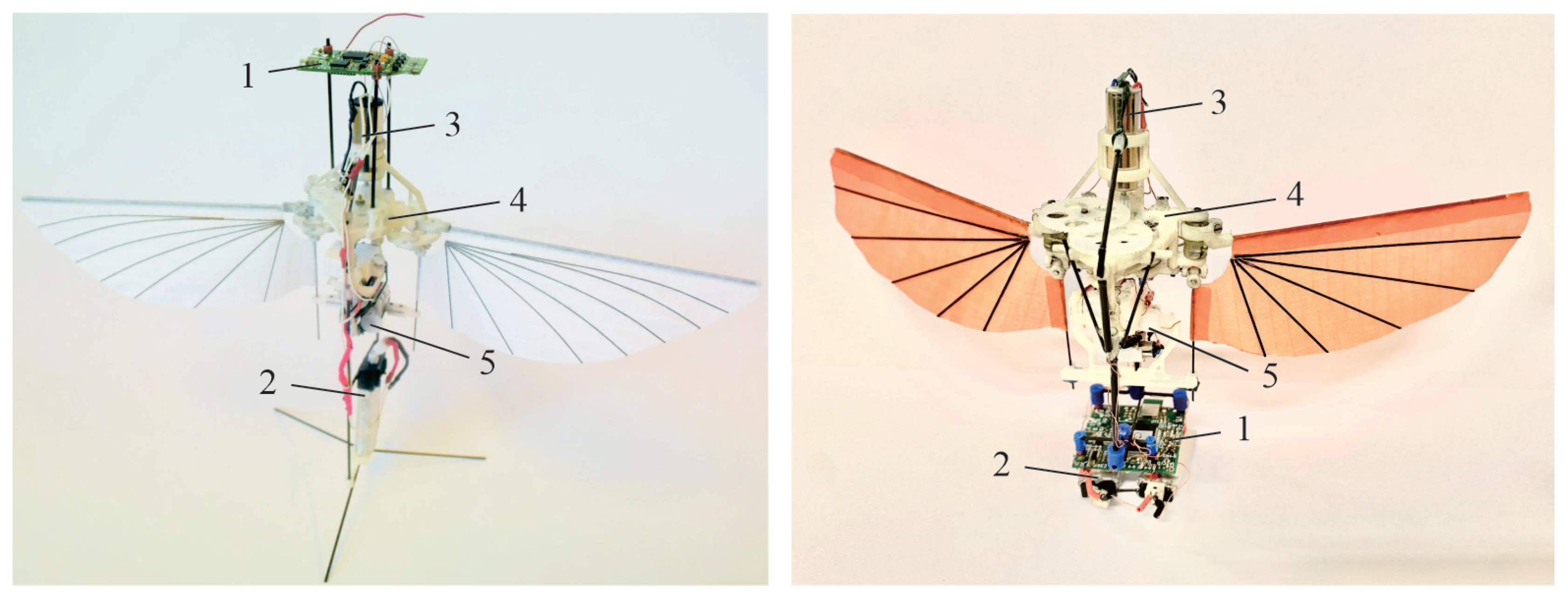
The general architecture of the Colibri robot has been described in earlier publications. It will not be repeated here, but a short video provides a visual summary [14]. Figure 1 shows a general view of the robot: an earlier version is presented on the left side (with the control board on top) [15,16,17], and a more recent prototype is shown on the right side, with the control board and the batteries located at the bottom [18]. The current weight is 22–23 g, depending on the configuration ( approximately twice that of the natural bird of the same size [19]), and the hovering flight autonomy is nearly 5 min.
Figure 1.
The robot Colibri. Left: early version with the control board on top [16]. Right: current configuration with the control board at the bottom. (1) Flight control board, (2) batteries, (3) main motor, (4) gearbox and flapping mechanism, (5) attitude control actuators.
2.1. Assumptions and Previous Results
- 1.
- The low-frequency dynamics (<10 Hz) can be modeled as those of a rigid body.
- 2.
- In hovering flight, the coupling between the longitudinal (pitch) and lateral dynamics (roll) is weak and can be neglected; therefore, they can be treated as independent. The roll, pitch and yaw axes may be assumed to be principal axes of inertia.
- 3.
- Because the flapping frequency is high (near 22 Hz), compared to the robot dynamics, the complex aerodynamic forces generated by the flapping wings may be approximated by their cycle-averaged values. The rapid changes in lift, drag and pitch moment during a flapping cycle can be treated as periodic noise. The flapping noise is mainly associated with the longitudinal dynamics; the drag noise and the pitch moment noise amplitudes are significantly larger than their average values and they have multiple harmonics. Due to the left–right symmetry, the lateral axis is not affected by significant flapping noise.
- 4.
- The longitudinal (pitch) and lateral (roll) axes are naturally unstable. When the center of drag is located above the center of mass (), both axes exhibit a pair of complex poles with positive real parts. They can be stabilized by a Proportional-Derivative (PD) compensator.
- 5.
- The vertical (yaw) axis is naturally stable. The vertical velocity is controlled by the flapping frequency ( as we are mainly interested in horizontal flights). The rotation about the yaw axis was not controlled in the hovering flights conducted so far [18] and a slow rotation was observed during the flight tests [20], as a consequence of a small asymmetry between the drag forces of of the left and right wings.
- 6.
- The robot is equipped with two inertial measurement units, IMUs (only one of them is currently used). Each IMU includes three gyroscopes measuring the three rotation velocities along the body axes, and three accelerometers sensing the three components of the specific acceleration (absolute acceleration minus gravitational acceleration). In hovering, the absolute acceleration vanishes (except for noise) and the specific acceleration indicates the direction of the gravity vector in the robot’s frame, .
- 7.
- The gyroscope output can be used directly in the PD controller of the longitudinal and lateral axes, but the attitude angles (roll and pitch) are not directly available; they must be reconstructed by independent dynamic state observers (one per axis). Dynamic state observers were successfully implemented as steady-state Kalman filters (based on assumptions regarding the system and sensor noise). This topic is discussed extensively in [18].
- 8.
- The PD controllers can indeed stabilize the pitch and roll axes but, because of the strong flapping noise, the drift of the robot cannot be avoided, making station keeping impossible. However, the full state dynamic observers allow the reconstruction of the longitudinal and lateral velocities in the robot frame, . This allows a significant improvement in station keeping via an outer proportional–integral (PI) control loop. It was implemented successfully and the performances observed were as good as earlier tests with an external tracking system (in spite of the slow uncontrolled rotation about the yaw axis) [18].
- 9.
- The full state observer (SO) worked surprisingly well during the previous hovering flight tests. Lightly damped flexible systems using full state observers are subject to a phenomenon known as “spillover” [21], in which the high frequency dynamics (flexible modes) neglected in the observer design tend to destabilize the system. This phenomenon was not observed in the hovering flight tests because of the large aerodynamic damping of the robot’s flexible modes.
2.2. Objectives of the Study
The aim of this study is to extend hovering flight control to trajectory tracking in a manner similar to that of quadcopters. This requires a third control loop on the yaw axis, leading to three independent loops for roll, pitch, and yaw, which are sufficient to follow slow trajectories. However, in order to follow fast horizontal trajectories, some kind of loop interaction must be introduced to handle the centrifugal forces during quick turns, mimicking the behavior observed in birds that lean towards the inside when turning. This introduces a nonlinear coupling between the three axes and a modification of the SO of the roll axis.
The paper is organized as follows: Section 3 recalls the control model of the longitudinal (pitch) axis already presented in [18]. Section 4 discusses the control model of the lateral (roll) axis, including the centrifugal acceleration; the modified state observer (MSO) for the roll axis is the main original contribution of the paper. Section 5 describes the control model of the yaw axis. Section 6 compares trajectories obtained when including the centrifugal acceleration with those obtained when it is neglected.
The following notations are used:
- (a)
- are the components of the velocity of the center of mass in the robot frame.
- (b)
- are the components of the angular velocity in the robot frame.
- (c)
- are the roll, pitch, and yaw attitude angles (Bryan).
3. Longitudinal (Pitch) Axis Control Model
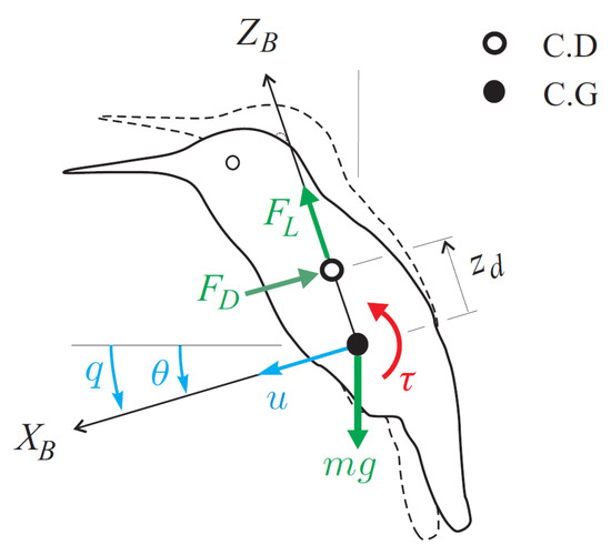
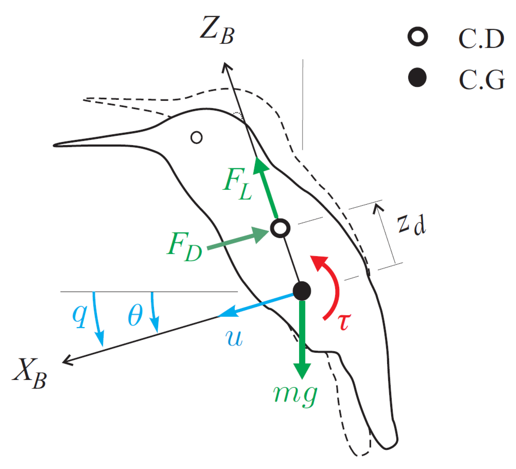
According to the assumptions introduced in the previous section, the longitudinal dynamics are governed by the Newton–Euler equations. The main damping mechanism is the flapping of the wings, which can be modelled accurately as a viscous damping. The drag force is proportional to the velocity of the centre of drag (Figure 2),
where u is the linear velocity of the centre of mass, and q is the pitch angular velocity. The damping constant K is a linear function of the flapping frequency. Assuming that the pitch attitude angle is small, so that and , Newton’s equation becomes
with , and
Figure 2.
Longitudinal (pitch) model of the robot near-hovering. Coordinate system, force and moment diagram. is the drag force, is the lift force, and .
Similarly, Euler’s equation governing the rotation about the centre of mass is
where is the drag moment and is the control torque obtained by twisting the wings via control bars actuated by servos. The actuator dynamics can be modelled as a first-order system with time constant T,
where is the requested torque.
In state-space form, the cycle-averaged longitudinal dynamics become
where and are always negative and and are negative if , that is, if the center of drag is above the center of mass, and positive if . The above equation includes the flapping drag noise d and the pitch flapping torque noise that enter the system at the input.
3.1. Output Equation
The IMU MEMS sensor is located at a distance above the center of mass ( above and below). The output consists of three gyroscopes measuring the angular velocity about the three body axes, and three accelerometers measuring the three components of the specific acceleration, .
For near-hovering horizontal flight, the quantities of interest are and q. The pitch rate q is one of the state variables, while can be expressed as
3.2. Stabilization, Station Keeping
Equations (5) and (7) have the classical state-space form
with the state vector , is the requested control torque, and is the process noise vector, representing the drag and torque disturbances produced by the flapping of the wings.
The open-loop longitudinal dynamics are unstable. For (centre of drag above the centre of mass), the pole configuration consists of a pair of unstable oscillatory poles and two stable poles on the negative real axis. The system can be stabilized with a PD controller. In the Laplace form,
or equivalently,
where is the pitch attitude error and q is the pitch angular velocity.
The pitch velocity q is directly available from the gyroscopes, whereas the pitch angle must be reconstructed from the sensor outputs . This can be achieved in several ways (e.g., by means of a complementary filter), but a full-state dynamic observer (Luenberger observer [22]) offers several advantages, which will become apparent below.
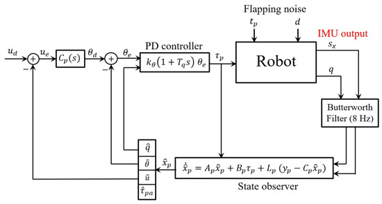
The stabilization loop is the inner loop shown in Figure 3. Here, denotes the desired pitch angle, while and are the estimated pitch angle and pitch rate, respectively. The observer gain matrix L is selected to provide a suitable compromise between observer bandwidth and noise attenuation. It can also be obtained as the steady-state gain of a Kalman filter by assuming suitable process and measurement noise statistics [18].
Figure 3.
Control of the longitudinal axial axis. The inner loop, based on PD control of q and , provides attitude stabilization. The outer loop provides station keeping by regulating the longitudinal velocity.
The inner stabilization PD loop described above stabilizes the longitudinal dynamics. However, it is very sensitive to IMU misalignment. A small calibration error in the pitch angle produces a non-zero pitch command , which in turn generates an axial velocity u. The steady-state velocity value results from the equilibrium between the off-axis component of gravity and the aerodynamic drag force .
Setting in (2) gives
which indicates that, when the robot moves forward with a uniform velocity, the robot leans forward in such a way that the longitudinal component of the lift vector balances the drag force while the vertical component balances the weight of the robot.
Since the full-state dynamic observer provides an estimate of the axial velocity , an outer control loop can be added (Figure 3), where is the desired longitudinal velocity ( at hovering) and is an appropriate compensator. Using a PI control
has been found to be very effective in flight tests [18].
4. Lateral (Roll) Axis Control Model
4.1. State-Space Model
In hovering flight, the lateral axis can be modelled in the same way as the longitudinal axis, leading to a set of three independent models (the yaw axis will be considered in the next section). However, for horizontal flight () dominated by the longitudinal direction () with sharp turns about the yaw axis (), the centrifugal acceleration may become a significant contributor to Newton’s equation of motion. Being the product of the longitudinal velocity u and the yaw velocity r, the term introduces a coupling between the three axes. It is the price to pay for mimicking birds that lean into turns.
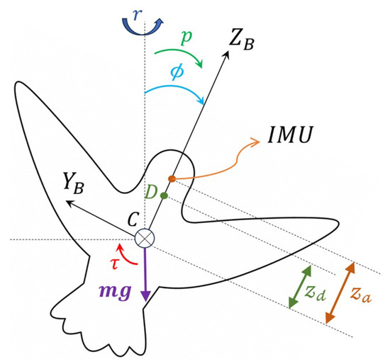
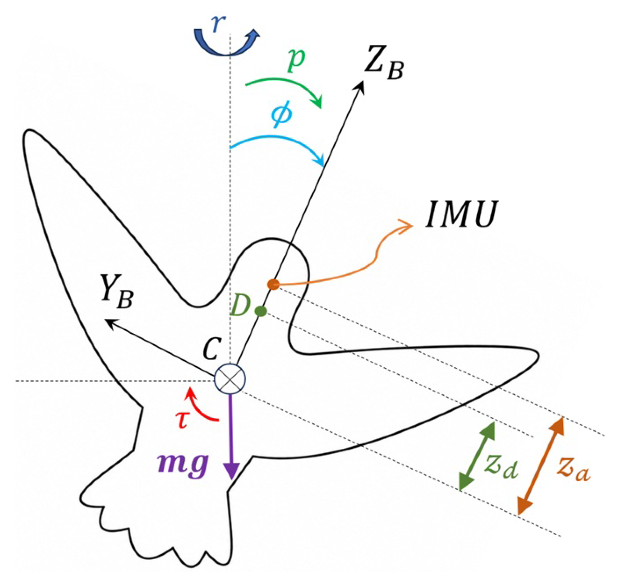
With the notation of Figure 4, the velocity of the center of drag is . With the foregoing assumptions, the y-component of Newton’s equation of motion in the robot frame becomes
with and . The Euler equation is similarly written as
where , , and is the roll control torque.
Figure 4.
Lateral (roll) model of the robot. The robot is seen from the back; the roll angle indicates the rotation about the body-fixed axis, and .
After moving the centrifugal force to the right-hand side of (14), the lateral dynamics can be written in state-space form as
where the centrifugal acceleration is treated as an external input. The normalized coefficients
have the same meaning as those introduced in Equation (5).
To illustrate the meaning of the additional centrifugal acceleration in Equation (14), consider a circular trajectory of radius R along which the robot rotates about the vertical axis with angular velocity r. The longitudinal velocity is
According to Equation (14), if there is no sideslip () and no roll rate (), the steady-state roll angle is
Therefore, the robot leans into the turn so that the lateral component of gravity balances the centrifugal acceleration.
4.2. Output Equation
The output of the accelerometer (lateral acceleration) is
Upon substituting and from the state-space model (16), the accelerometer output becomes
This equation cannot be written in the usual output equation form because of the unknown centrifugal acceleration term . However, using the estimates and available from the pitch and yaw models, the accelerometer output can be modified as
The new output vector, , takes the classical form
where . The estimation error of the centrifugal acceleration can be regarded as noise.
4.3. Observer Equation
Equations (16) and (22) can be written in the standard state-space form as
where , represents the centrifugal acceleration acting as an external disturbance, and .
Using an MSO, the state estimate can be expressed as follows:
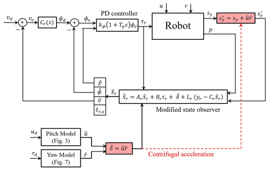
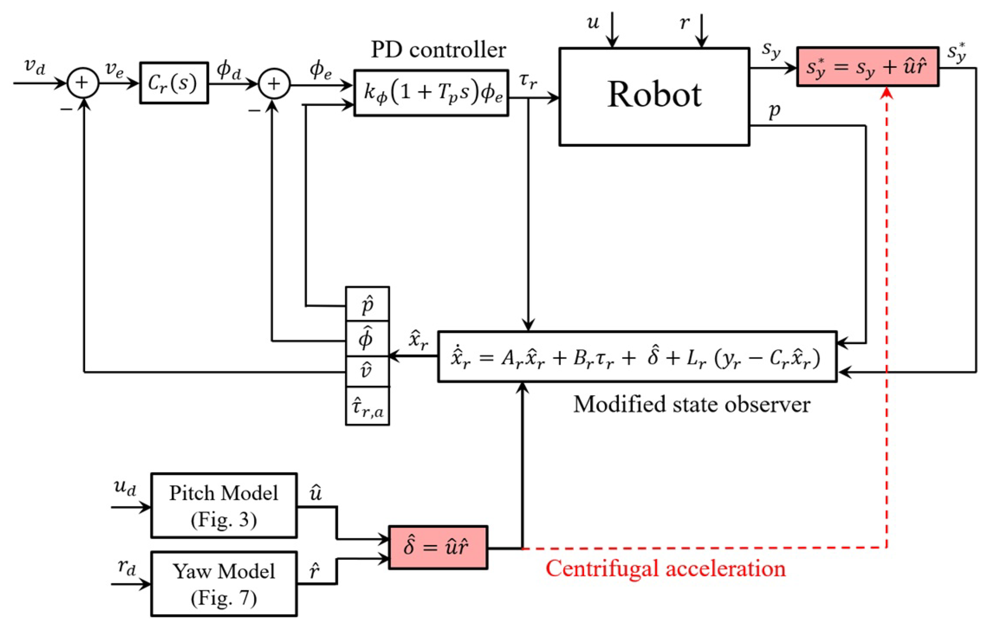
where is an estimate of the disturbance vector , obtained from the estimated longitudinal velocity and yaw rate provided by the pitch observer, together with the output of the Butterworth filter (BF) in the yaw control system.
The state estimation error satisfies
If is Hurwitz (i.e., all its eigenvalues have negative real parts), the observer error is exponentially stable in the absence of disturbance-estimation and measurement errors. More generally, if and are bounded, the estimation error remains bounded. Asymptotic convergence, , is achieved when and .
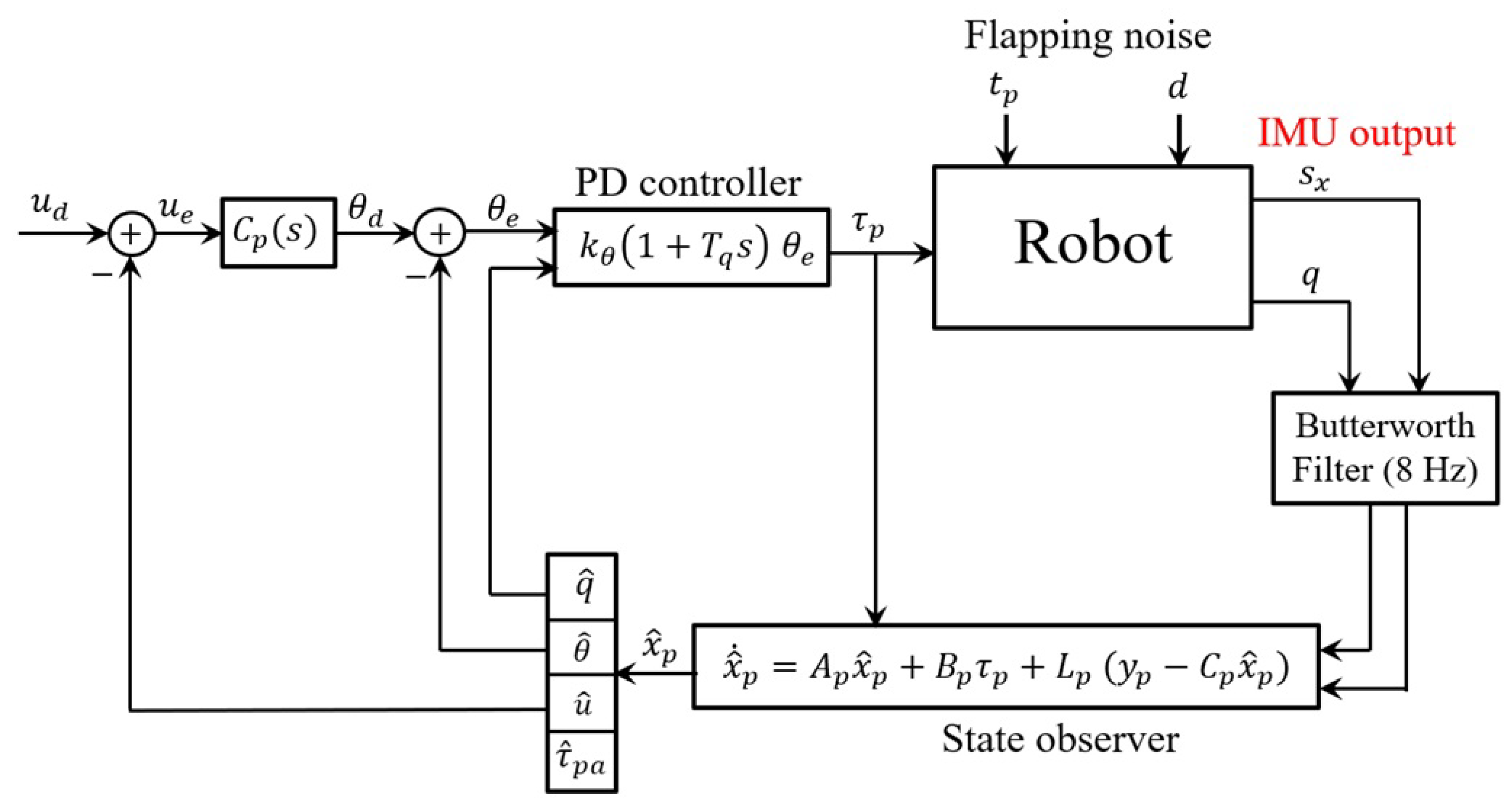
The block diagram of the roll axis control system is shown in Figure 5. The PD controller used for the stabilization loop and the compensator that converts the desired lateral velocity into a desired roll angle are essentially identical to those employed for the pitch axis.
Figure 5.
Control of the roll axis including the centrifugal accelerations. , , and are desired values of the longitudinal, lateral, and yaw (spin) velocities.
5. Yaw Axis Control Model
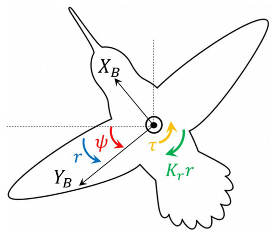
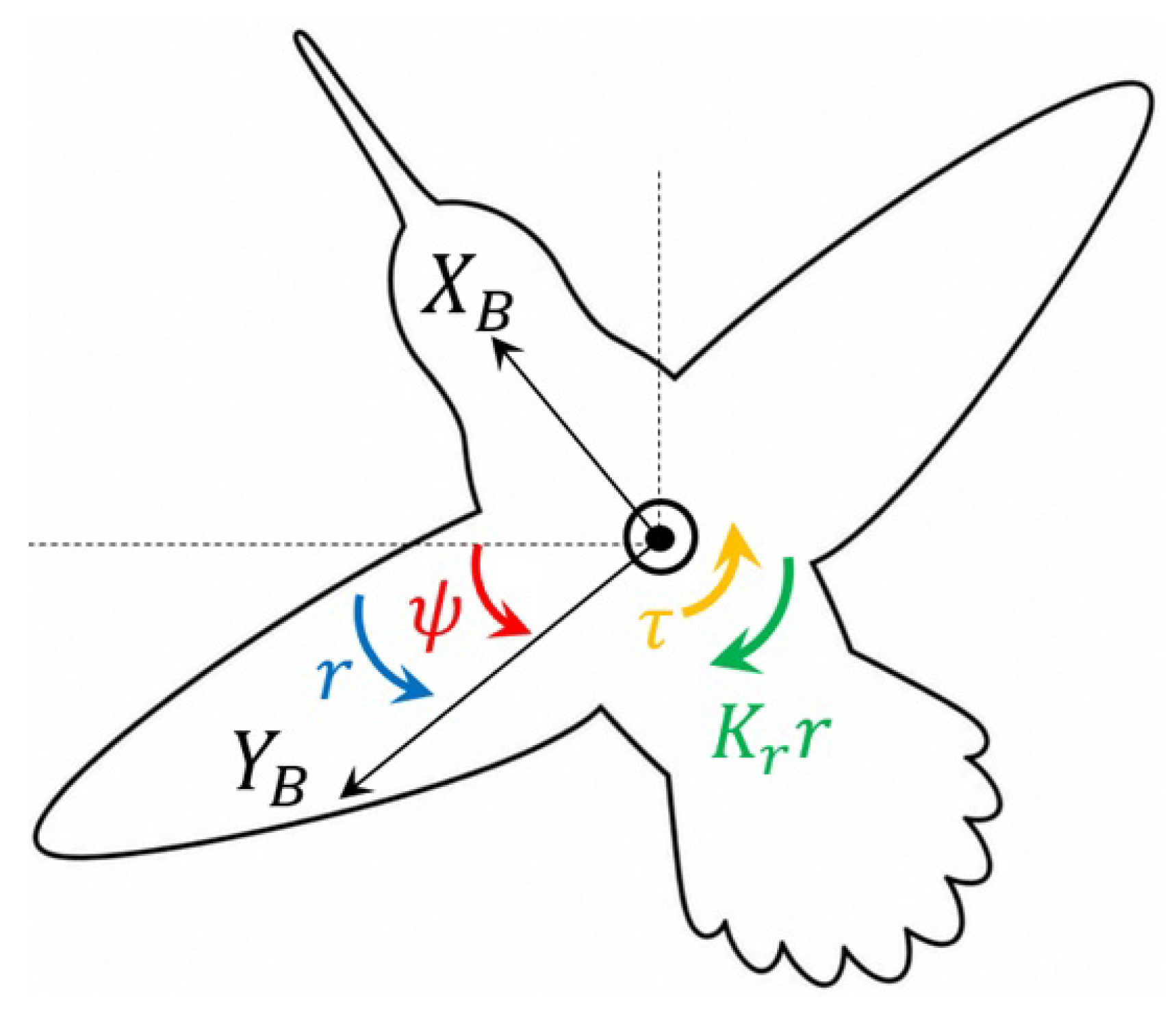
With the notations of Figure 6, the yaw dynamics read
where is the yaw velocity (spin), is the moment of inertia about the axis, and is the rotational damping coefficient about the yaw axis. is the control torque obtained by varying the drag force of the left and right wings ( is estimated from a pendulum experiment).
Figure 6.
Coordinates of yaw dynamics. Robot seen from above.
As for the pitch and roll control torque, the wing twist is obtained by a servo actuator modeled by a first-order system with a time constant T (Equation (4)). In state-space form, the yaw dynamics become
where , and is the requested torque. The yaw velocity r is directly available from the IMU; therefore, it does not require a SO. We introduce a second-order low-pass BF to attenuate the noise from the gyroscope.
The open-loop transfer function between the requested torque and the yaw velocity is
Using a PI controller,
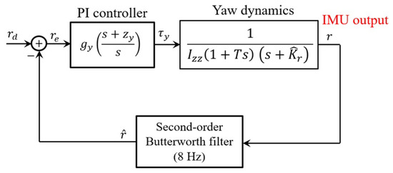
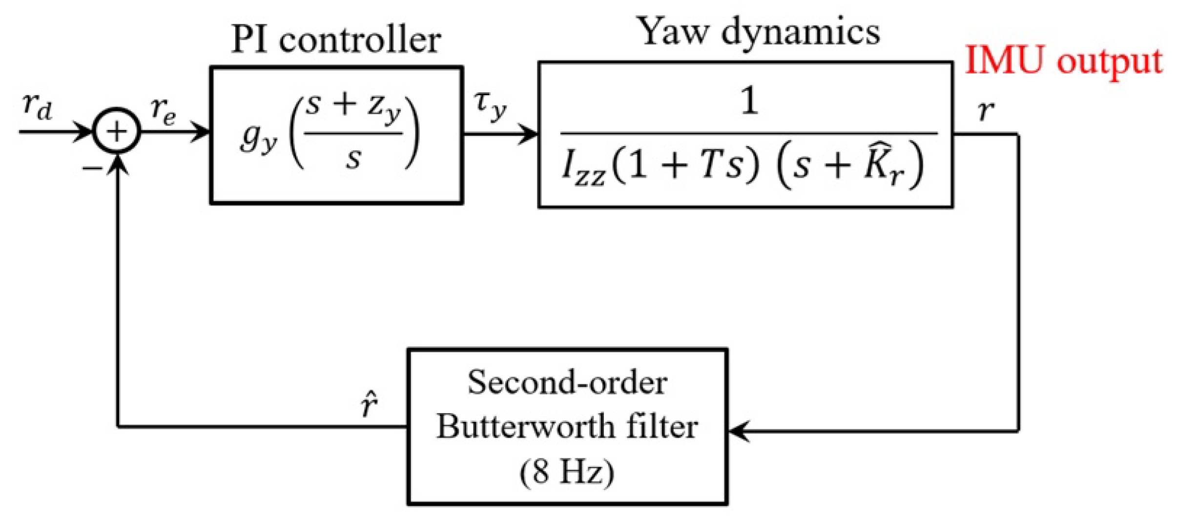
The control block diagram is shown in Figure 7.
Figure 7.
Control flowchart of yaw dynamics using PI control and a low pass Butterworth filter.
6. Numerical Simulation
The following simulation studies evaluate the tracking performance of the proposed controller for two horizontal reference trajectories: (i) a circular trajectory and (ii) a Gerono lemniscate trajectory. In both cases, the desired motion is specified in the robot frame by the velocity vector and the desired yaw rate . In the MATLAB/Simulink simulations, the sampling time was set to , and the fourth-order Runge–Kutta method was employed to solve the closed-loop system.
For the flapping disturbances, the measured drag force and pitch torque signals are downsampled and transformed into the frequency domain using the FFT. Frequency components above 50 Hz are removed, and the filtered time-domain disturbances are reconstructed using the inverse FFT and periodically repeated as simulation inputs.
6.1. Circular Trajectory
To evaluate the proposed control architecture, consider the open-loop generation of a circular trajectory starting from rest with a radius of , travelled in . The corresponding input data for the three axes of the robot frame are m/s, and rad/s. During the trajectory, the robot is subject to a centrifugal acceleration m/s2.
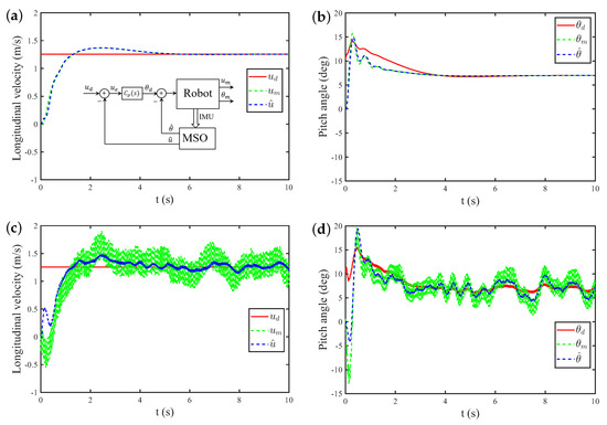
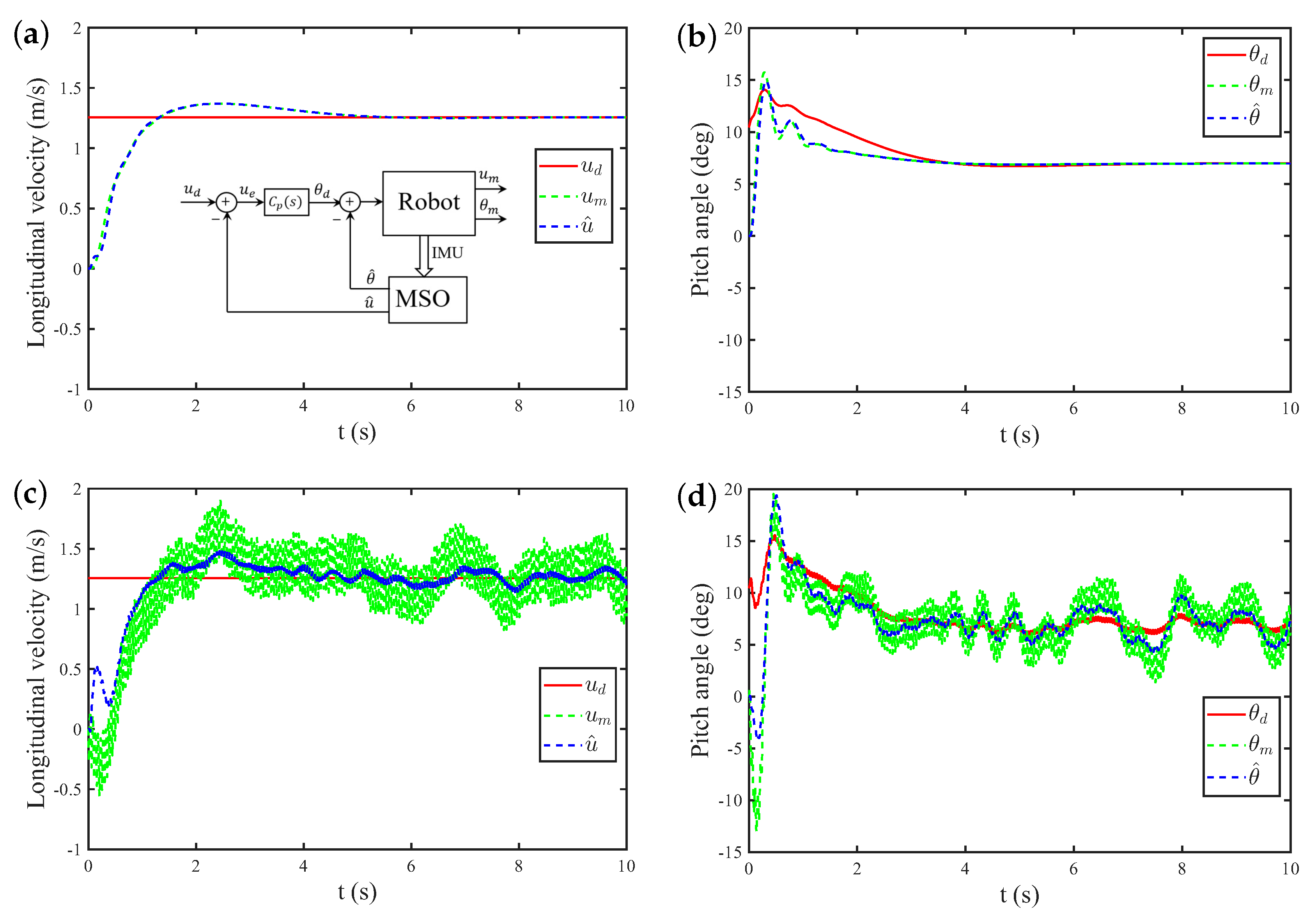
With reference to Figure 5, the robot model for the roll axis is Equation (16) including the centrifugal acceleration. Figure 8 gives the state responses of the pitch system. Figure 8a,b show the longitudinal velocity and the pitch attitude angle in the absence of flapping noise. Figure 8c,d show the effect of the flapping noise (see Appendix B).
Figure 8.
State responses of the pitch system while tracking a circular trajectory. (a,b) show the responses by the state observer (SO) and without flapping noise, whereas (c,d) include the effects of torque noise and drag noise d in the longitudinal (pitch) dynamics. The meaning of the various subscripts is explained in the block diagram on the top left figure. The subscripts (d) and (m) denote the desired command and the measured (actual) system state, respectively, while the superscript () indicates the state estimated by the state observer (SO).
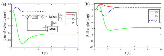
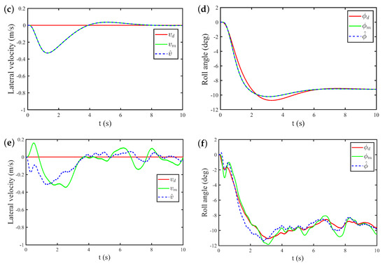
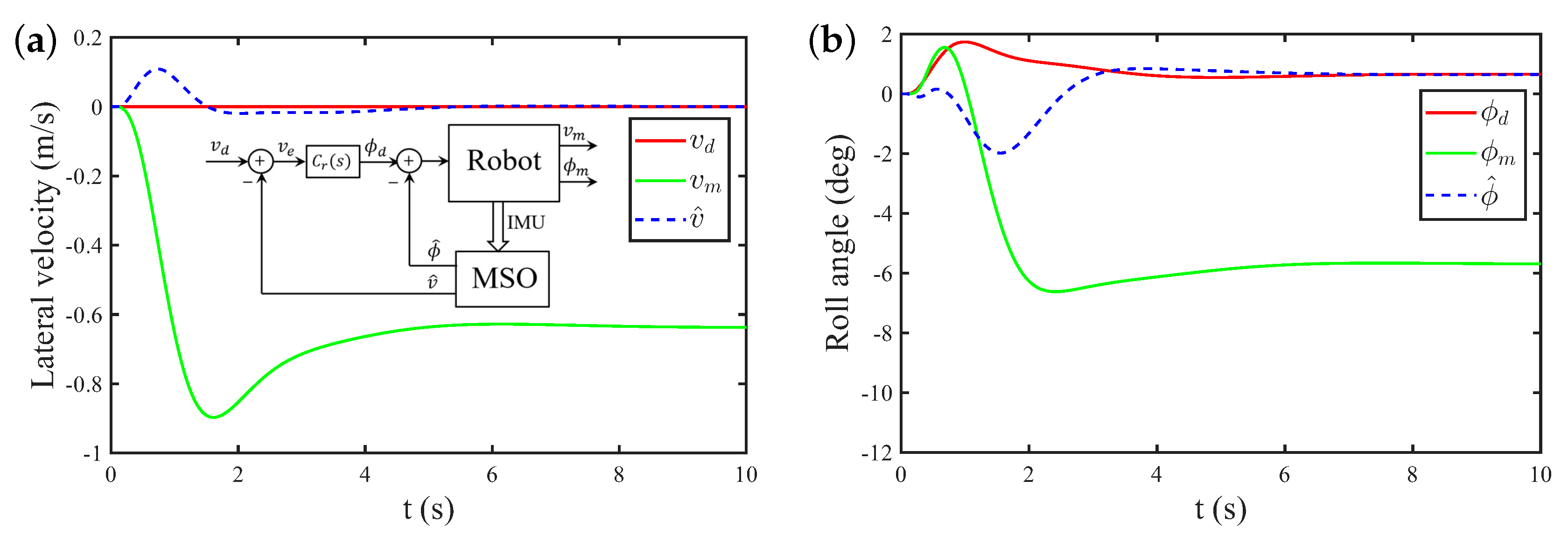
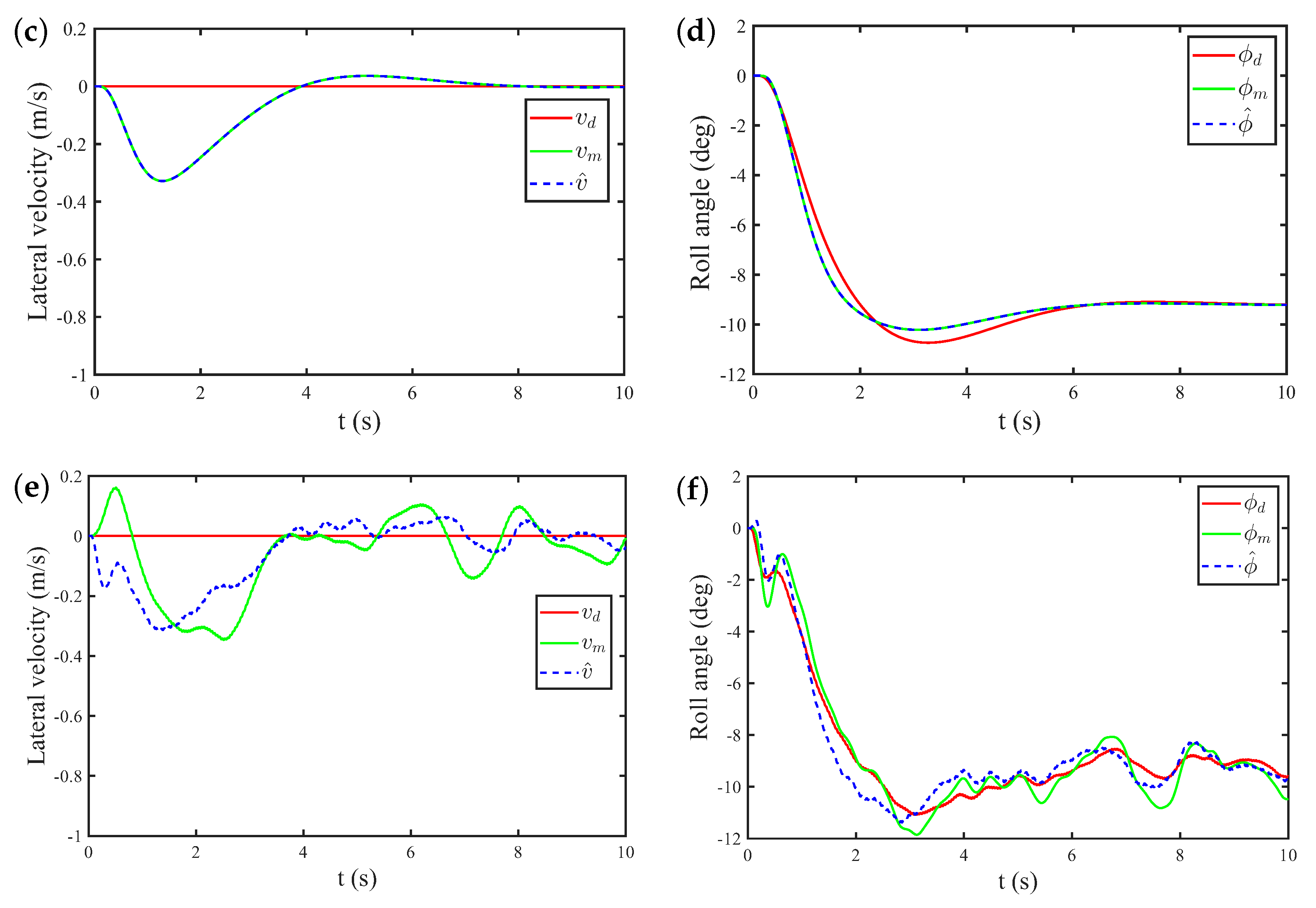
Figure 9 compares the results obtained with MSO with those obtained with SO assuming independent treatment of the three axes (when the centrifugal acceleration is neglected). We observe that, with the MSO, the estimated values and follow closely the output of the robot model, and , and converge toward the desired value. On the other hand, with the classical SO (independent observers), a significant sideslip velocity occurs.
Figure 9.
State responses of the roll system while tracking a circular trajectory. (a,b) show the results when the centrifugal acceleration is not included in the observer estimation (SO). (c,d) show the results with the modified state observer (MSO) including the centrifugal acceleration and (e,f) show the same results when the flapping noise ( and d) is applied to the longitudinal (pitch) dynamics.
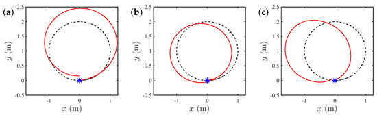
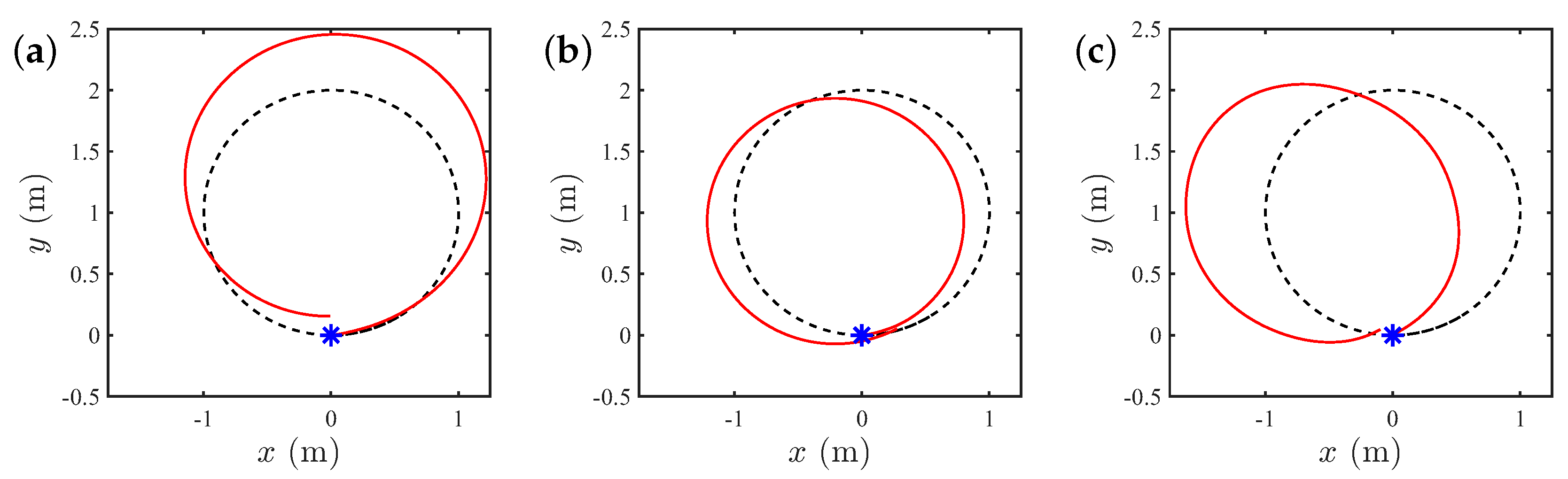
Figure 10 shows the trajectory obtained in absolute frame when generating , and in robot frame. From left to right, (a) the roll dynamics observer ignores the centrifugal acceleration (SO), resulting in a side slip velocity responsible for an increase of the circle diameter; (b) the observer of the roll dynamics includes the centrifugal acceleration (MSO); and (c) the flapping noise is included in the analysis with MSO.
Figure 10.
Circular trajectory generated in robot frame and seen in inertial frame; the target is indicated in black dashed line. (a) presents the result obtained assuming no interaction between axes (SO); (b) shows the result including the interaction due to centrifugal acceleration (MSO); and (c) illustrates the MSO result when the flapping noise ( and d) is applied to the longitudinal (pitch) dynamics.
6.2. Lemniscate Trajectory
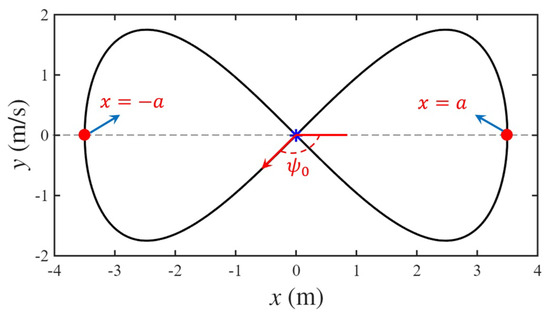
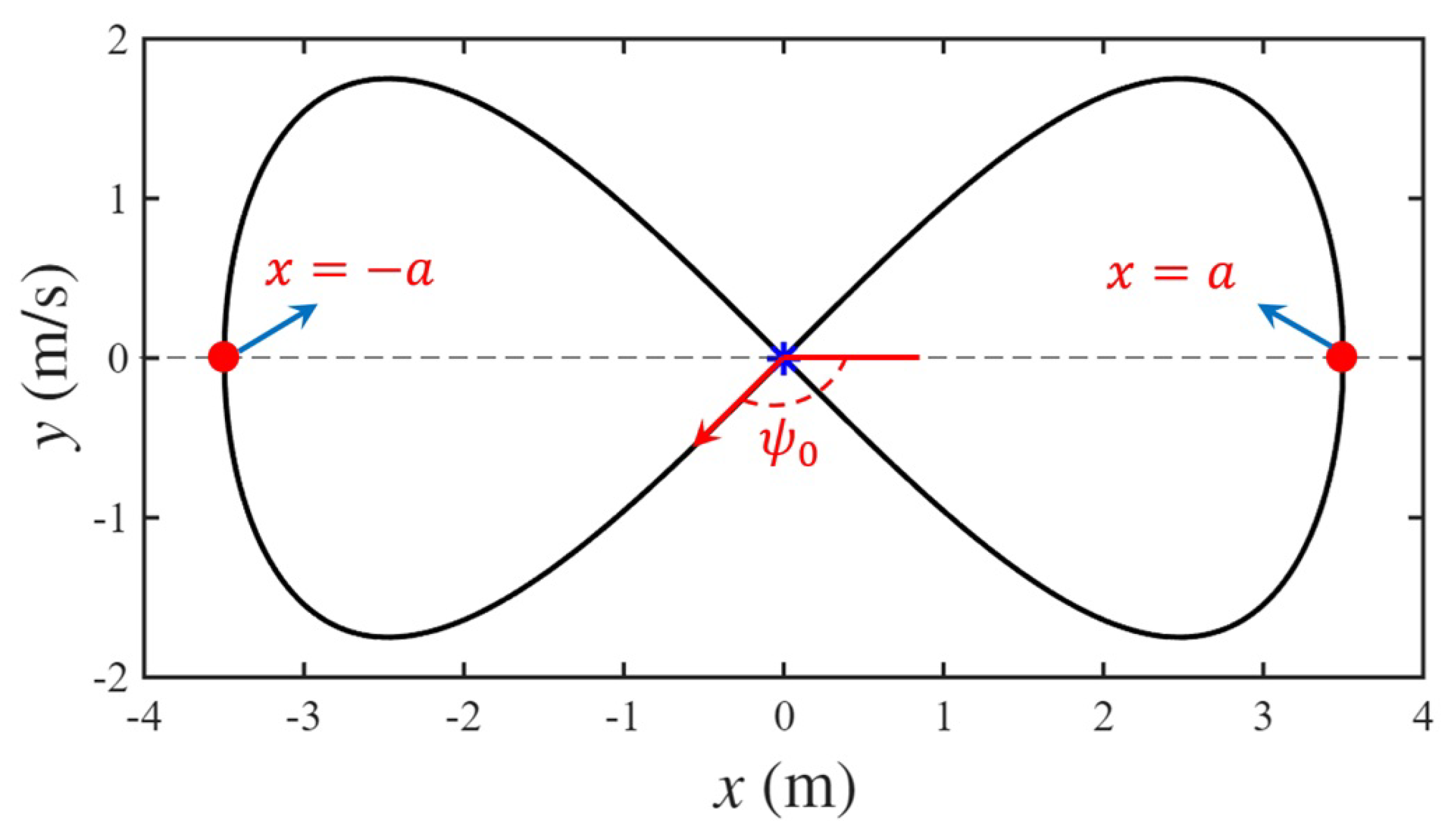
The reference trajectory is generated using a Gerono lemniscate, which provides smooth and continuous changes in curvature with alternating turning directions. The trajectory is defined as
where a is the scaling factor (or amplitude) that determines the physical size of the curve, and is a real number that typically ranges from 0 to radians (Figure 11).
Figure 11.
Lemniscate trajectory. The point denotes the initial position, represents the initial heading angle, and is the scaling factor.
The corresponding reference inputs in the robot body-fixed frame are a constant surge velocity of m/s, zero sway velocity (), and a time-varying yaw rate is obtained by differentiating the desired heading angle, , which is computed from the tangent direction of the reference trajectory. The time parameterization of the Gerono lemniscate is given by
where . The resulting trajectory is subsequently re-parameterized by arc length and traversed at a constant forward speed of .
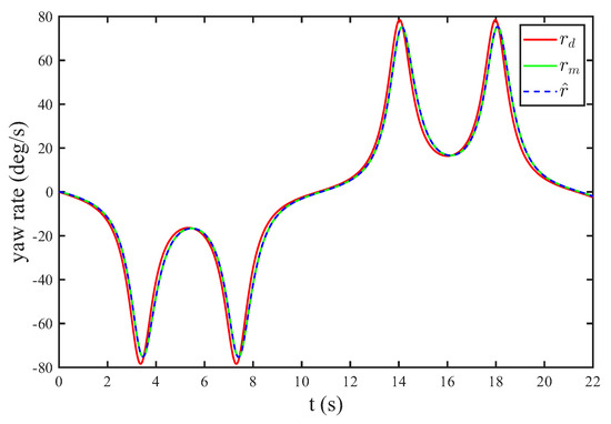
Figure 12 illustrates the response of yaw system during lemniscate following. The figure shows that the measured yaw rate accurately follows its reference with a high accuracy steady-state tracking performance, resulting in a smooth heading evolution that generates the required lemniscate motion.
Figure 12.
State responses of the yaw system for following a lemniscate trajectory.
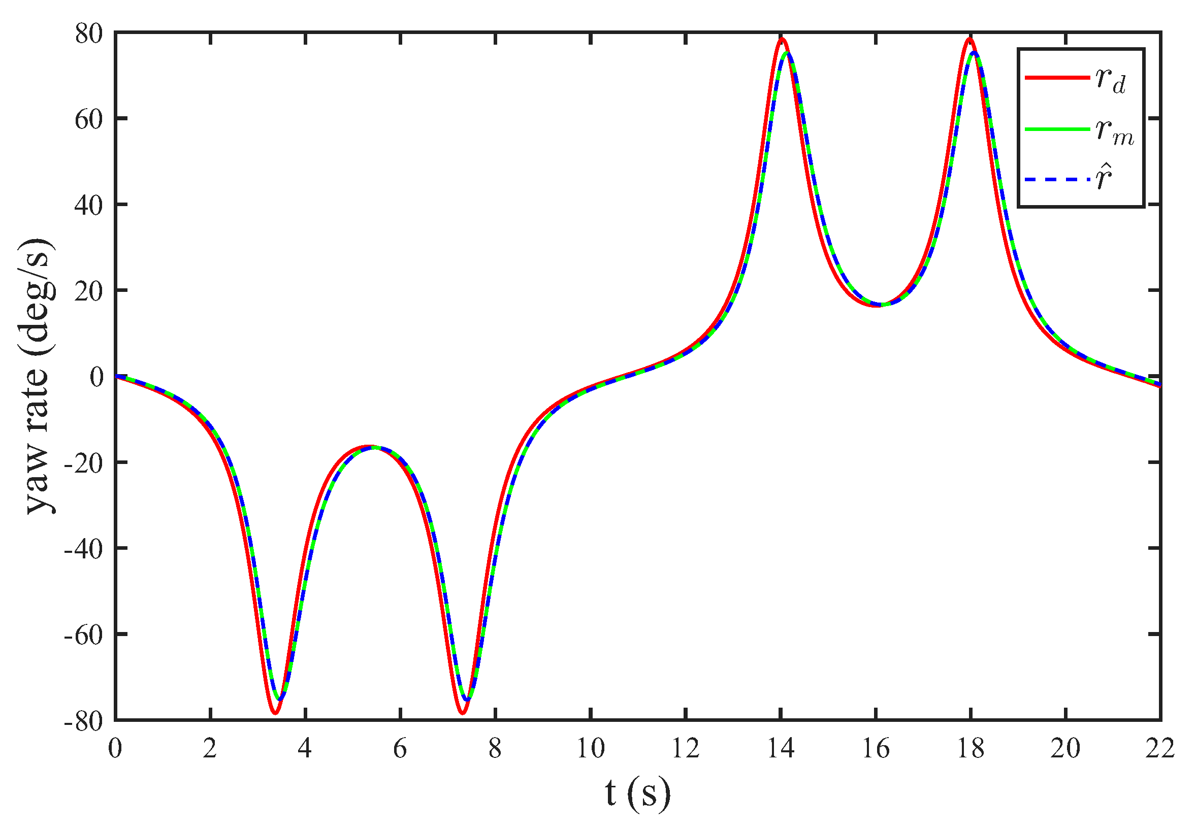
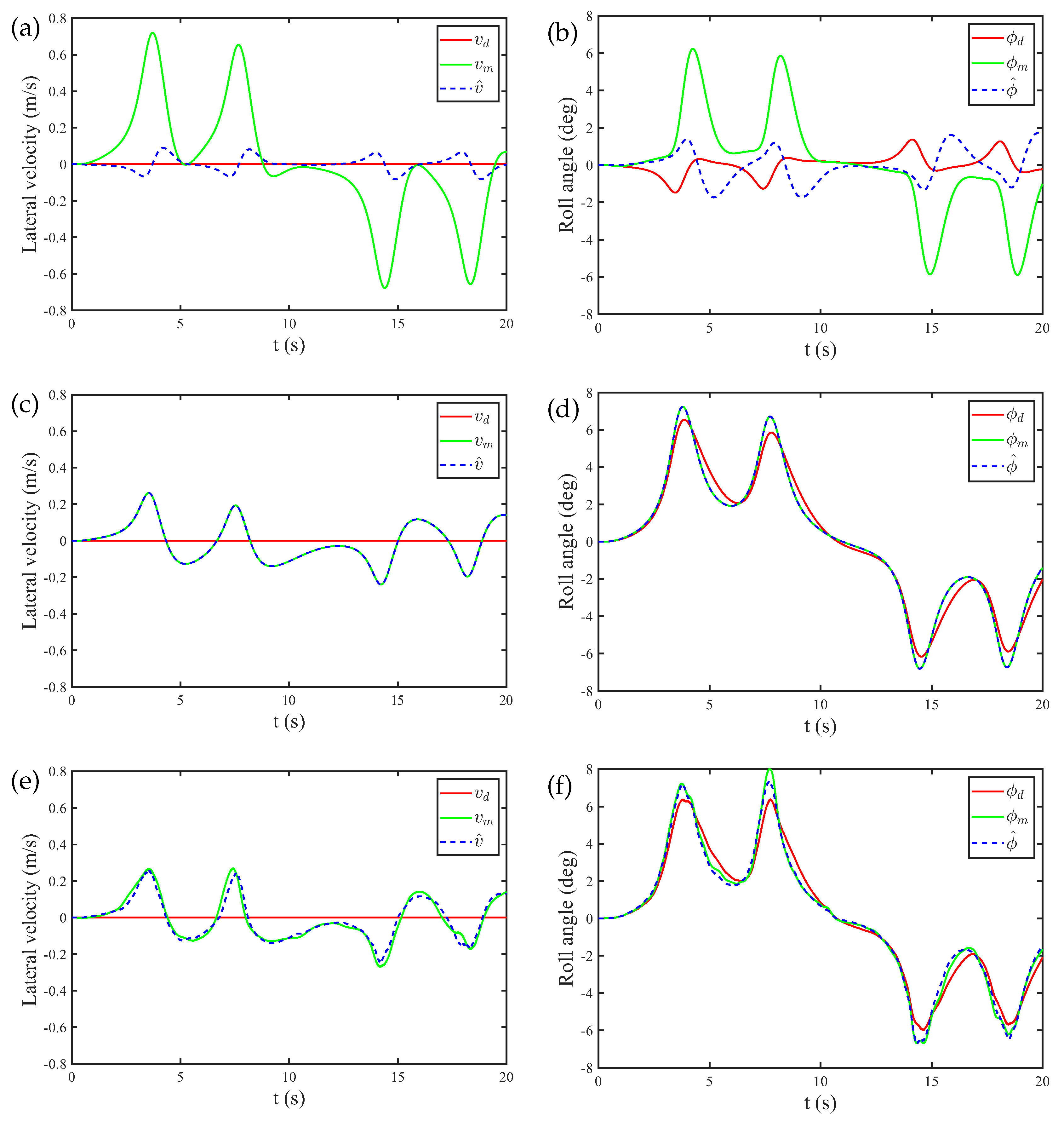
The state responses of the roll system are shown in Figure 13. Similar to the circular trajectory case, incorporating the estimation of the centrifugal acceleration compensation significantly improves the estimation of the lateral velocity and roll angle. The estimated states closely follow the model responses, whereas neglecting the coupling introduces noticeable tracking errors.
Figure 13.
State responses of the roll system while tracking a lemniscate trajectory. (a,b) show the results when the estimation of centrifugal acceleration is not included in SO. (c,d) show the results with MSO. And (e,f) show the same results when the flapping noise ( and d) is applied to the longitudinal (pitch) dynamics.
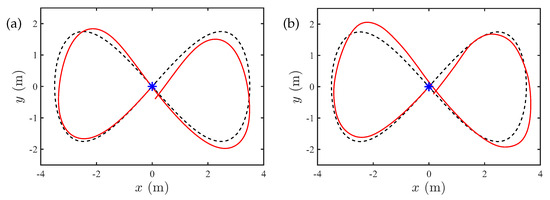
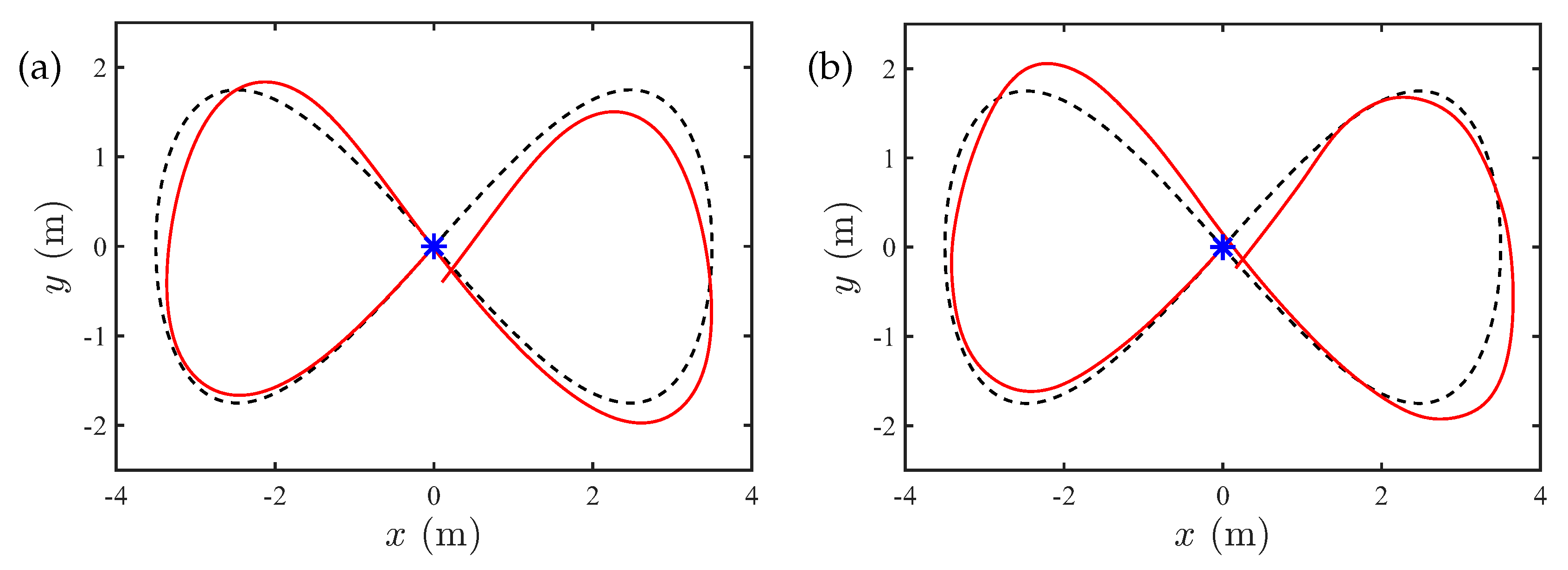
Finally, Figure 14 presents the resulting trajectory in the inertial frame. The proposed MSO achieves accurate tracking of the lemniscate motion under nominal conditions, as depicted in Figure 14a. When flapping-related perturbations are incorporated into the pitch dynamics, the tracking performance is slightly affected; however, the hummingbird robot continues to follow the reference trajectory with satisfactory accuracy, as shown in Figure 14b.
Figure 14.
Lemniscate trajectory following in the absolute frame. (a) shows the results with MSO and (b) shows the same result when the flapping noise ( and d) is applied to the longitudinal (pitch) dynamics.
7. Conclusions
The paper presents an extension of the control strategy for hovering flight to horizontal trajectories by specifying the velocity vector (, , ) in the robot frame. The state of the system is reconstructed from on-board inertial measurements. The centrifugal acceleration encountered in sharp turns is accounted for by introducing a coupling between the pitch–roll–yaw axes in a modified state observer for the roll axis. The control strategy is assessed numerically. In steady-state conditions (constant forward velocity , , and constant yaw rate ), the forward component of the lift vector is such that it balances the drag force, while its lateral component balances the centrifugal acceleration. Flight experiments are in preparation to validate the idea. In the absence of centrifugal acceleration, the MSO is identical to the classical observer SO, which has been tested successfully in [18]; the additional computational burden of the MSO is minimal and should not pose implementation problems.
Author Contributions
Conceptualization, A.P.; software, Y.F.; validation, Y.F. and A.P.; original draft preparation, A.P.; writing, review and editing A.P. and Y.F.; supervision, A.P. All authors have read and agreed to the published version of the manuscript.
Funding
This research received no external funding.
Institutional Review Board Statement
Not applicable.
Informed Consent Statement
Not applicable.
Data Availability Statement
The original contributions presented in this study are included in the article. Further inquiries can be directed to the corresponding author.
Conflicts of Interest
The authors declare no conflict of interest.
Abbreviations
The following abbreviations are used in this manuscript:
| FWMAV | Flapping-Wing Micro-Air Vehicle |
| IMU | Inertial Measurement Unit |
| MEMS | Micro-Electro-Mechanical System |
| SO | State Observer |
| MSO | Modified State Observer |
| RMS | Root Mean Square |
| FFT | Fast Fourier Transform |
| PD | Proportional Plus Derivative |
| PI | Proportional Plus Integral |
| BF | Butterworth Filter |
Appendix A. COLIBRI Parameters Used in the Dynamics Model
The simulation results in this paper are based on the data provided in [15] and summarized in Table A1. It is assumed that roll and pitch systems have the same damping coefficients K and . The controller and observer gains for the roll, pitch, and yaw systems are provided in Table A2.
Table A1.
COLIBRI parameters for the body dynamics model.
Table A2.
Control/observer parameters of the roll, pitch, and yaw systems.
Appendix B. Flapping Noise (Drag and Pitch Torque)
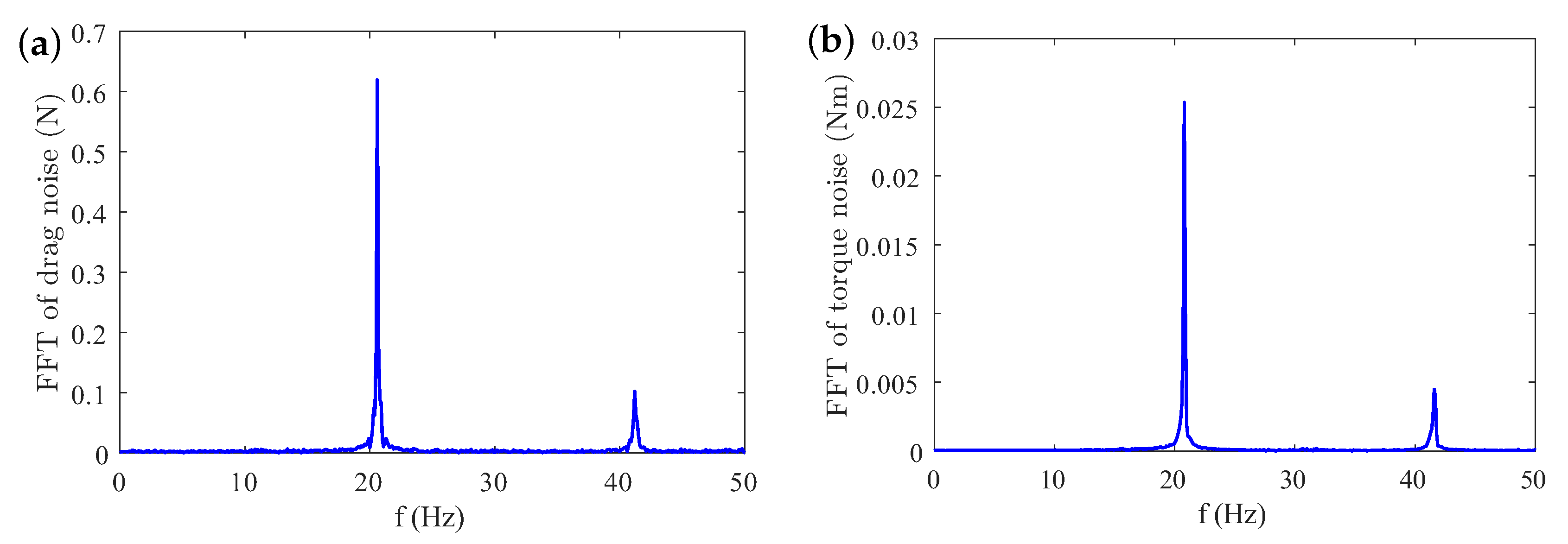
The high-frequency components of the aerodynamic forces generated during the flapping of the wings are neglected in a cycle-averaged model. In this study, they are treated as periodic noise. Because of the left–right symmetry of the robot system, only the axial (pitch) dynamics are significantly affected by the flapping noise. The harmonic components were estimated in an earlier study by attaching the robot to a force sensor to measure the axial noise d and to a torque sensor to estimate the pitch torque . Although rigidly holding the robot against the sensor is not fully representative of the aerodynamic forces in free flight, we have assumed that the first two components are the same (flapping frequency and first harmonic) and the higher harmonics are neglected. With this assumption, the RMS value of the drag force is reduced from 0.985 N to 0.5 N and that of the pitch torque from 0.0273 Nm to 0.0210 Nm. These values are still quite high (the average lift is 0.2 N and the maximum control moment is 0.002 Nm). The FFT components are shown in Figure A1; the first peak corresponds to the flapping frequency, the second harmonic is due to the complex aerodynamics during the upstroke and downstroke motions.
Figure A1.
Fast Fourier Transform (FFT) spectra of the drag noise d (a) and pitch torque noise (b), with peaks at the flapping frequency and its second harmonic due to the upstroke and downstroke.
References
- Xiao, S.; Hu, K.; Huang, B.; Deng, H.; Ding, X. A Review of Research on the Mechanical Design of Hoverable Flapping Wing Micro-Air Vehicles. J. Bionic Eng. 2021, 18, 1235–1254. [Google Scholar] [CrossRef] [Scilit]
- Ward, T.A.; Rezadad, M.; Fearday, C.J.; Viyapuri, R. A Review of Biomimetic Air Vehicle Research: 1984–2014. Int. J. Micro Air Veh. 2015, 7, 375–394. [Google Scholar] [CrossRef] [Scilit]
- Keennon, M.T.; Klingebiel, K.R.; Won, H.; Andriukov, A. Development of the Nano Hummingbird: A Tailless Flapping Wing Micro Air Vehicle. In Proceedings of the 50th AIAA Aerospace Sciences Meeting including the New Horizons Forum and Aerospace Exposition, Nashville, TN, USA, 9–12 January 2012; pp. 1–24. [Google Scholar]
- Phan, H.V.; Park, H.C. Insect-Inspired, Tailless, Hover-Capable Flapping-Wing Robots: Recent Progress, Challenges, and Future Directions. Prog. Aerosp. Sci. 2019, 111, 100573. [Google Scholar] [CrossRef] [Scilit]
- Phan, H.V.; Aurecianus, S.; Au, T.K.L.; Kang, T.; Park, H.C. Towards Long-Endurance Flight of an Insect-Inspired, Tailless, Two-Winged, Flapping-Wing Flying Robot. IEEE Robot. Autom. Lett. 2020, 5, 5059–5066. [Google Scholar] [CrossRef] [Scilit]
- Coleman, D.; Benedict, M. Methods for Stabilizing the Longitudinal Dynamics of a Biomimetic Robotic Hummingbird in Hovering Flight. Int. J. Micro Air Veh. 2025, 17, 1–17. [Google Scholar] [CrossRef] [Scilit]
- Tu, Z.; Fei, F.; Zhang, J.; Deng, X. An At-Scale Tailless Flapping-Wing Hummingbird Robot. I. Design, Optimization, and Experimental Validation. IEEE Trans. Robot. 2020, 36, 1511–1525. [Google Scholar] [CrossRef] [Scilit]
- Hyun, N.-S.P.; McGill, R.; Wood, R.J.; Kuindersma, S. A New Control Framework for Flapping-Wing Vehicles Based on 3D Pendulum Dynamics. Automatica 2021, 123, 109293. [Google Scholar] [CrossRef] [Scilit]
- Zheng, H.; Chen, W.; Xie, F. Control Simulation of Flapping-Wing Micro Aerial Vehicle Based on Multi-Level Optimization Model Predictive Control. IEEE Access 2024, 12, 40700–40709. [Google Scholar] [CrossRef] [Scilit]
- Nguyen, K.; Au, L.T.K.; Phan, H.-V.; Park, H.C. Comparative Dynamic Flight Stability of Insect-Inspired Flapping-Wing Micro Air Vehicles in Hover: Longitudinal and Lateral Motions. Aerosp. Sci. Technol. 2021, 119, 107085. [Google Scholar] [CrossRef] [Scilit]
- Fei, F.; Tu, Z.; Zhang, J.; Deng, X. Learning Extreme Hummingbird Maneuvers on Flapping Wing Robots. In Proceedings of the 2019 International Conference on Robotics and Automation (ICRA), Montreal, QC, Canada, 20–24 May 2019; pp. 109–115. [Google Scholar] [CrossRef] [Scilit]
- Tu, Z.; Fei, F.; Zhang, J.; Deng, X. Acting Is Seeing: Navigating Tight Space Using Flapping Wings. In Proceedings of the 2019 International Conference on Robotics and Automation (ICRA), Montreal, QC, Canada, 20–24 May 2019; pp. 95–101. [Google Scholar] [CrossRef] [Scilit]
- Sarkar, D.; Hyun, N.-S.P. Leveraging Flapping Kinematics for Attitude Estimation in SO(3). In Proceedings of the 2025 IEEE 64th Conference on Decision and Control (CDC), Rio de Janeiro, Brazil, 9–12 December 2025; pp. 7449–7456. [Google Scholar] [CrossRef] [Scilit]
- Colibri Project. Available online: https://www.youtube.com/watch?v=I2ih-Q1IKDc (accessed on 20 August 2026).
- Roshanbin, A. Design and Development of a Tailless Robotic Hummingbird. Ph.D. Thesis, Université Libre de Bruxelles, Department of Control Engineering and System Analysis, Bruxelles, Belgium, September 2019. [Google Scholar]
- Roshanbin, A.; Altartouri, H.; Karasek, M.; Preumont, A. COLIBRI: A Hovering Flapping Twin-Wing Robot. Int. J. Micro Air Veh. 2017, 9, 270–282. [Google Scholar] [CrossRef] [Scilit]
- Roshanbin, A.; Abad, F.; Preumont, A. Kinematic and Aerodynamic Enhancement of a Robotic Hummingbird. AIAA J. 2019, 57, 4599–4607. [Google Scholar] [CrossRef] [Scilit]
- Wang, H.; Farid, Y.; Wang, L.; Garone, E.; Preumont, A. Hovering Flight of a Robotic Hummingbird: Dynamic Observer and Flight Tests. Actuators 2024, 13, 91. [Google Scholar] [CrossRef] [Scilit]
- Greenwalt, C.H. Hummingbirds; Dover: New York, NY, USA, 1990. [Google Scholar]
- Station Keeping. Available online: https://youtu.be/53DJ0rtebKk (accessed on 20 August 2026).
- Balas, M.J. Active control of flexible systems. J. Optim. Theory Appl. 1978, 25, 415–436. [Google Scholar] [CrossRef] [Scilit]
- Luenberger, D. An Introduction to Observers. IEEE Trans. Autom. Control 1971, 16, 596–602. [Google Scholar] [CrossRef] [Scilit]
Disclaimer/Publisher’s Note: The statements, opinions and data contained in all publications are solely those of the individual author(s) and contributor(s) and not of MDPI and/or the editor(s). MDPI and/or the editor(s) disclaim responsibility for any injury to people or property resulting from any ideas, methods, instructions or products referred to in the content. |
© 2026 by the authors. Licensee MDPI, Basel, Switzerland. This article is an open access article distributed under the terms and conditions of the Creative Commons Attribution (CC BY) license.