


Abstract
This study applies a Craig–Bampton (CB) substructure reduction procedure to the prediction of natural frequency changes upon rotor replacement in a shaft generator shafting system and quantifies its accuracy and computational cost for that configuration. Because the shafting conditions are determined by the customer, performing full finite element analysis or experimental modal analysis (EMA) for every design change is impractical. The shafting system is divided into shaft and rotor substructures, and CB reduced-order models are constructed independently for each substructure. A three-stage verification framework—FE analysis versus EMA, the CB reduced-order model versus FE analysis, and the CB reduced-order model versus EMA—is employed to separate FE model error from CB reduction error. The CB pipeline reproduced the bending modes of the assembly with a maximum error of 0.26% against the parent finite element model, with a subspace MAC of 1.0000 for every mode group below 720 Hz, while reducing the model from 192,678 to 5379 degrees of freedom. With 20% of the interface degrees of freedom retained, the first three bending modes are predicted within 0.60%, and the reduced model comprises 1173 degrees of freedom, a reduction of 99.39%. The first bending mode error varies monotonically with the retention level, and the errors of all three bending modes remain bounded below 0.60% down to 20% retention. For the annular interface examined, the error-retention relation, therefore, provides a quantitative basis for selecting a retention level against a stated error tolerance, but its extension to other interface topologies, mesh densities, and mode ranges remains to be established.
1. Introduction
A shaft generator is a rotating machine integrated into a ship’s propulsion shafting system. Unlike a conventional standalone machine—where the manufacturer controls the entire rotor–stator–shaft–support design—a shaft generator is connected to propulsion shafting, whose layout and boundary conditions are determined incrementally by the shipyard customer. Consequently, the shaft and coupling conditions are not fixed at the time of rotor design, and full dynamic characterization of the assembled system cannot be performed independently by the manufacturer [1].
This product reality creates two compounding difficulties. First, at the early design stage, customer shafting information arrives in a limited or evolving form, making it impossible to build a complete FE model of the full assembly. Second, even when the assembly model is available, performing a fresh full-system FEA or EMA for every rotor variant—a routine occurrence given customer-driven design iterations—is time-consuming and commercially impractical [1].
Dynamic substructuring addresses both difficulties by decomposing the system into substructures, characterizing each substructure independently, and predicting full-assembly dynamics by coupling the substructure models through interface conditions [2,3]. When one component changes, only the corresponding substructure model needs to be updated—the rest of the library is reused unchanged. Among substructure coupling methods, the Craig–Bampton (CB) method [4] is the dominant choice for engineering practice because it retains boundary (interface) DOFs as physical coordinates while reducing only the interior DOFs to a truncated set of fixed-interface normal modes and constraint modes. This makes substructure coupling algebraically straightforward and computationally efficient.
A body of prior work has established the accuracy and versatility of CB-based substructuring. Roettgen et al. [5] compared multiple ROM techniques—including CB—for beam and cylinder–plate–beam assemblies and found CB to be reliable across configurations. Jin et al. [6] applied component mode synthesis to force identification at the system level. Allen et al. [7] demonstrated that interface modeling quality governs coupling accuracy when the junction consists of flexible fixtures or multipoint connections. Hybrid experimental–analytical variants, in which some substructures are characterized by measured FRFs rather than FE models, have also been explored extensively [8]. The transmission simulator (TS) concept [9] is a prominent example, though it can introduce spurious modes that limit its robustness [5].
Interface reduction has been addressed through several families of methods. A posteriori schemes compress the interface after an auxiliary analysis of the substructure’s own condensed interface matrices and include the generalized interface degrees of freedom of Balmès [10] and the characteristic constraint modes of Castanier et al. [11]. A priori schemes instead prescribe the reduced interface basis from the interface geometry alone [12,13,14], which allows the reduced-order model of each substructure to be built independently. Comparative evaluations of these families for rotor dynamic models have been reported recently [15].
In rotating machinery, component mode synthesis has been applied to rotor-bearing systems with fixed-free interfaces [16] and has been surveyed for rotor dynamic model reduction more broadly [17], while interface reduction has been extended to nonlinearly coupled systems [18]. What these applications share is that the interface basis, once reduced, no longer corresponds to identifiable physical locations on the coupling surface.
The present work belongs to this family but differs in the choice of basis: the reduced interface is a Boolean subset of the physical interface nodes rather than a set of polynomial or harmonic functions, so the retained coordinates remain identifiable physical locations. The closest prior work is that of Tran [19], whose partial interface modes retain a subset of interface nodes but supplement them with interface modes to maintain full compatibility; here, the removed nodes are instead reclassified as interior degrees of freedom and partial compatibility is accepted as a quantified trade-off. Existing a priori bases are functional in form, whether polynomial [13] or derived from an auxiliary structure [20]. This paper offers a quantitative investigation of interface representation for axisymmetric shaft–rotor couplings, together with a sampling criterion that makes the required number of retained nodes independent of mesh density.
For the assembly examined, with 20% of the interface nodes retained, the first three bending modes are predicted within 0.60% of the parent finite element model, while the assembled reduced model contains 1173 degrees of freedom, a reduction of 99.39%. Because the prediction error varies monotonically with the retention level, the error-retention relation can be used to select a retention level for interfaces of this type. The present evidence covers one annular interface, one mesh, and the first three bending modes.
The remainder of the paper is organized as follows. Section 2 provides the theoretical background: dynamic substructuring, DOF partitioning, the CB transformation, and the TS concept. Section 3 describes the experimental system, FE model configuration, and the first verification stage (FEA vs. EMA). Section 4 details the CB ROM construction procedure, the substructure assembly algorithm, and the DOF reduction statistics. Section 5 presents results: CB accuracy relative to ANSYS Modal (2025 R2), final prediction accuracy relative to EMA, error source analysis for the outlier mode, and—centrally—the interface DOF sensitivity study, and closes with the scope and limitations of the study. Section 6 draws conclusions and identifies directions for future work.
2. Theoretical Background
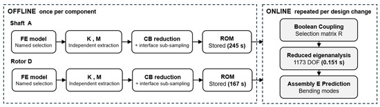
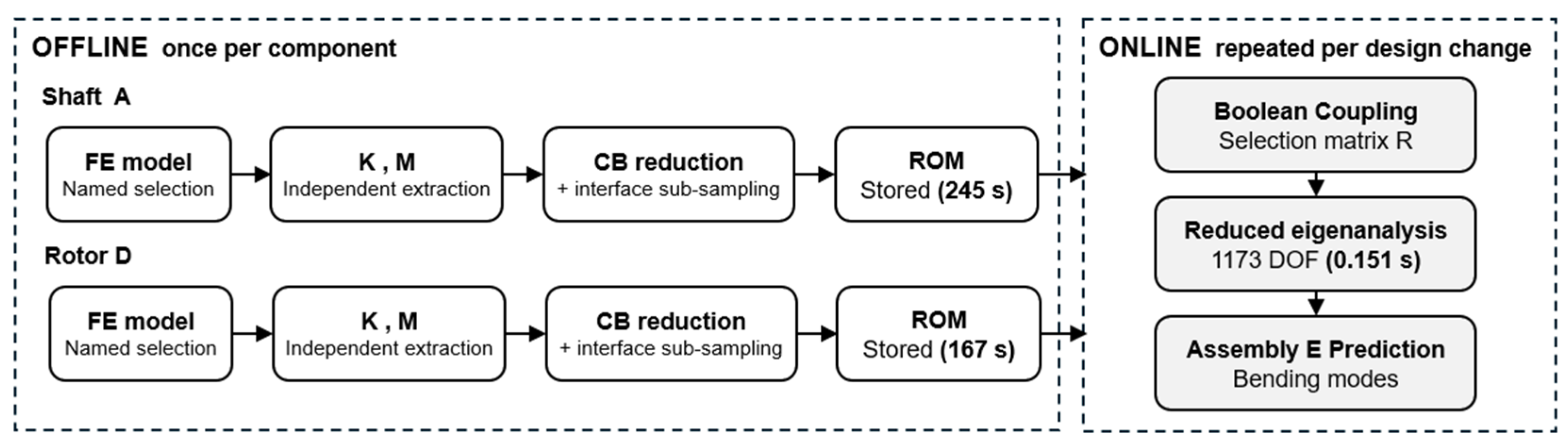
The procedure is organized into two stages. The offline stage denotes the component-level reduction performed once per substructure, in which the mass and stiffness matrices are extracted, the fixed-interface normal modes and constraint modes are computed, and the reduced-order model is stored. The online stage denotes the coupling of the stored models and the solution of the reduced eigenvalue problem, repeated whenever a component is replaced. The two stages differ in how often they are executed, and it is the online stage that determines the cost of a repeated design study.
2.1. Substructure Partitioning and DOF Classification
Dynamic substructuring decomposes a complex structural system into substructures, characterizes each independently, and predicts full-assembly dynamics through interface coupling [2,3]. The key advantage is modularity: when one substructure changes, only its ROM needs to be rebuilt—all other substructure models remain valid and can be reused. This makes the method particularly attractive for products such as shaft generators, where the rotor is a replaceable component while the shaft and support structure are fixed.
Previous studies have demonstrated substructure coupling for diverse configurations: beam assemblies, cylinder–plate–beam systems, and force identification problems [5,6]. A natural extension is the hybrid experimental–analytical approach, in which substructures with difficult-to-model joints are characterized by measured FRFs while the remainder of the assembly is represented analytically. The TS method [9] is a prominent realization, though spurious modes can arise depending on the number of retained modes and measured DOFs [5]. The present study restricts itself to the purely analytical CB framework and the TS method is discussed in Section 2.3 as background for future extensions.
In substructure coupling, the process of dividing the entire system into appropriate substructures must precede, and the DOFs of each substructure are classified into interior DOFs and boundary DOFs. Interior DOFs are DOFs defined only within the corresponding substructure, and boundary DOFs are interface DOFs connected to other substructures.
For substructure coupling, the physical coordinate vector of each substructure can be classified into interior DOFs and boundary DOFs, which is expressed as Equation (1):
Here, denotes the interior DOF vector and denotes the boundary DOF vector. The mass matrix M and stiffness matrix K are partitioned into interior–interior, interior–boundary, and boundary–boundary blocks according to the same DOF classification, as expressed in Equations (2) and (3). Here, the subscript i denotes interior DOFs and b denotes boundary DOFs:
In this study, the coupling portion of the shaft and rotor is defined as the interface region. That is, the DOFs at the position where the two substructures are connected are set as boundary DOFs, and the remaining regions are classified as interior DOFs. This definition allows the same interface conditions to be applied during subsequent reduction and reassembly while maintaining the physical meaning of the substructures.
2.2. Craig–Bampton Method
The Craig–Bampton method is a representative model order reduction technique used in substructure coupling [4,21]. Its most important characteristic is that while boundary DOFs are maintained as physical coordinates, only interior DOFs are converted to a reduced coordinate system. Therefore, the interface DOFs necessary for coupling between substructures can be directly retained while reducing the total number of DOFs.
In the Craig–Bampton method, the physical coordinates of a substructure are represented by a combination of two types of basis functions, namely, fixed-interface normal modes and constraint modes. Fixed-interface normal modes represent the dynamic behavior of interior DOFs with all boundary DOFs fixed, and constraint modes represent the static deformation pattern occurring at interior DOFs when a unit displacement is applied to each boundary DOF.
The Craig–Bampton coordinate transformation is expressed as Equation (4):
Here, the transformation matrix TCB consists of fixed-interface normal modes and constraint modes, and is defined as Equation (5):
The constraint modes are obtained by imposing a unit displacement on one boundary degree of freedom while the remaining boundary degrees of freedom are held fixed, which gives the static response of the interior partition:
The fixed-interface normal modes are obtained from the eigenvalue problem of the interior partition with all boundary degrees of freedom fixed:
They are mass-normalized, which is the condition under which the modal block of the reduced mass matrix becomes the identity, as given in Equation (8):
In Equations (4) and (5), is the fixed-interface normal mode matrix, is the constraint mode matrix, and represents the generalized coordinates for selected modes. Boundary DOFs remain as physical coordinates even after reduction, so interface DOF can be directly used when reassembling substructures.
Using the transformation matrix, the original mass matrix and stiffness matrix are expressed in reduced form as Equations (9) and (10), respectively:
Here, is the identity matrix and is the diagonal matrix consisting of the squares of fixed-interface natural frequencies. The fact that the interior–interior blocks of and simplify to the identity matrix and diagonal matrix, respectively, is an important characteristic of the Craig–Bampton method [22].
When assembling the Craig–Bampton models of two substructures and the compatibility condition for boundary DOFs is applied. The condition constraining the shared boundary DOF to perform the same motion is expressed as Equation (11):
Solving the eigenvalue problem from the equations of motion of the assembled full system using this condition yields the natural frequencies and mode shapes of the assembly.
When only a subset of the interface nodes is retained, the reduced boundary coordinates are obtained by a Boolean selection from the full boundary set:
Here, R is a Boolean selection matrix with exactly one unit entry per row and at most one per column, so the retained coordinates remain a subset of the physical interface degrees of freedom and the selection introduces neither interpolation nor a multipoint constraint. The identity = I holds for any such selection, whereas Pb = is a diagonal projector whose null entries identify the released degrees of freedom. The boundary degrees of freedom that are not retained are not removed from the model—they are reclassified as interior degrees of freedom and condensed together with the original interior partition. Writing Rc for the complementary selection formed from the deleted rows, the repartition is a permutation of the original ordering:
where collects the original interior degrees of freedom together with the released boundary degrees of freedom. The mass and stiffness matrices are transformed by the same permutation:
and Equations (4)–(10) are then applied to (, ) with the partition (i*, b*) without modification. The constraint modes and the fixed-interface normal modes are, therefore, recomputed at every retention level rather than obtained by selecting columns of the full interface basis.
Because the retained boundary coordinates of the two substructures are physical and identically ordered, the reduced-order models are coupled by a Boolean primal assembly. Collecting the modal coordinates of both substructures and the shared retained interface coordinates in a single generalized coordinate vector:
where L is Boolean, the assembled matrices follow by congruence:
No mass or stiffness matrix of the assembled model is required at any stage—only the two component-level reduced matrices and the Boolean map L enter Equation (16). Displacement compatibility is enforced strongly on the retained subset through Equation (15), whereas on the degrees of freedom annihilated by Pb in Equation (12) it is satisfied only in the sense of the condensed representation. This is a quantified trade-off rather than a preserved property, and Section 5.5 reports the resulting error as a function of the retention level.
2.3. Transmission Simulator
Although this study primarily utilizes the purely analysis-based CB method, the transmission simulator (TS) concept is an important theoretical background when considering future expansion to experiment-based substructure coupling. TS serves a role that helps better reflect the interface conditions that the substructure of interest experiences in the actual assembled state and is introduced to enhance interface dynamics in hybrid experimental–analytical substructure coupling [8].
The conceptual structure of the TS method analytically separates substructure A serving the transmission simulator role from the reference experimental system C, then combines a new substructure D to predict the final system. It can be conceptually understood in the form of C − A + D. Previous studies have proposed a method for estimating the dynamic characteristics of a substructure of interest from an existing experimental system through this procedure and predicting a new assembly by combining it with other analytical models [5]. However, the TS method may generate spurious modes depending on the number of selected modes and measured DOFs [5,9], so this study does not include the experiment-based technique in its scope and utilizes the purely analysis-based Craig–Bampton method as the primary framework.
In this study, the shaft generator shafting system is formalized as a problem of dividing into shaft and rotor substructures and combining different rotor models into the same shaft. The reference assembly is defined as the combination of shaft and rotor (1), and the prediction target assembly as a system combining rotor (2) to the same shaft. This study performs Craig–Bampton reduction at the substructure level for each assembly and constructs a procedure for predicting and verifying the change in assembly dynamic characteristics due to rotor replacement by comparing the results with ANSYS Modal analysis values and EMA measurements.
In this study, ANSYS Workbench serves as a tool for extracting mass matrices and stiffness matrices necessary for Craig–Bampton reduction, and ANSYS Modal analysis results are used for two purposes. First, in Section 3, they serve as the reference values for comparison with EMA measurement results to evaluate the validity of the finite element model. Second, in Section 4, they are used as the verification reference value for the Craig–Bampton reduced-order model constructed in the Python 3.14.7 environment. This usage does not conflict with the purpose of this study to predict dynamic characteristics without using ANSYS Modal analysis. The target to be replaced is the ANSYS Modal analysis that is repeatedly performed on the entire assembly for every design change, and ANSYS is limited to the stage of extracting mass-stiffness matrices once per substructure and generating the verification reference values for the reduced-order model.
3. System and Experimental Setup
This section defines the research target system and substructures and describes the finite element model configuration, the experimental modal analysis procedure, and the interface definition used for substructure coupling. Additionally, the first verification of this study, the comparison of ANSYS Modal analysis results with EMA measurement results, is performed to secure the reliability of the FE model. The FE model with secured reliability in this section is used as the base model for matrix extraction and CB reduction in Section 4.
3.1. Target System and Substructure Definition
The research target is a simplified shaft–rotor assembly of a shaft generator shafting system. As described in the introduction, since the boundary conditions of shaft generator products are structures determined in the intermediate process of design, it is difficult to fully verify the dynamic characteristics of the entire shafting at the early stage of the early design. Therefore, this study aims to construct a substructure coupling-based procedure that can predict dynamic characteristics under changed conditions without directly analyzing or testing the entire assembly repeatedly.
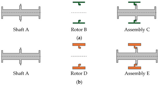
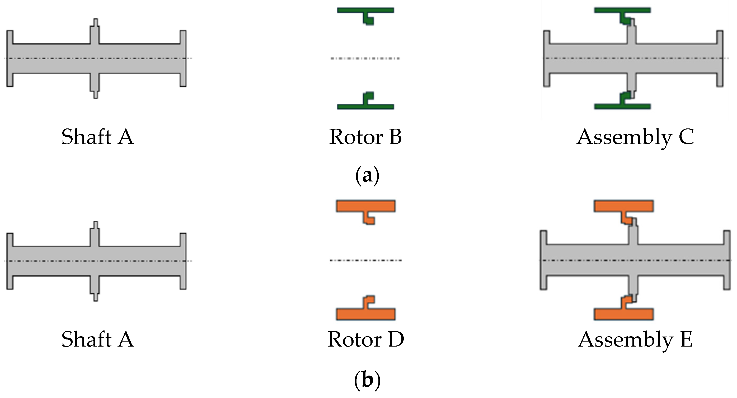
The research target system is defined as two substructures consisting of a shaft and rotor. Here, the shaft is set as the common substructure and the rotor as the replaceable substructure. As described in the introduction, due to experimental conditions, assemblies applying two rotors with different masses to the same shaft are set as the verification targets. The substructure definitions used in this study are shown in Table 1, and the individual substructure geometry and assembly structure are shown in Figure 1. The two rotors have the same coupling geometry capable of joining the same shaft but differ in mass and inertia properties.
Table 1.
Substructure and assembly definitions.
Figure 1.
Substructure geometry and assembly structure. (a) Shaft A, rotor B (rotor (1)), assembly C (shaft + rotor (1)). (b) Shaft A, rotor D (rotor (2)), assembly E (shaft + rotor (2)). Each rotor has the same coupling geometry but different mass properties: rotor (1) ≈ 3.1 ton and rotor (2) ≈ 3.5 ton.
In this study, to quantitatively analyze the effect of the mass difference between the two rotors on assembly dynamic characteristics, the mass of rotor (1) as the reference substructure is set to approximately 3.1 ton and the mass of rotor (2) as the replacement substructure to approximately 3.5 ton. Due to this mass difference, the two assemblies (C and E) sharing the same shaft have different natural frequency distributions, and this constitutes the verification target of the substructure coupling-based prediction procedure in this study.
The overall procedure of this study consists of analysis-based model construction, experimental modal analysis, substructure definition and interface setting, and verification of prediction results. First, finite element models are constructed for the shaft alone and two types of assemblies, and the natural frequencies and mode shapes of each system are calculated. Subsequently, experimental modal analysis is performed using the actual test specimen and compared with analytical results to review model validity. The shaft and rotor are then separated as substructures, the coupling DOFs are defined as the interface, and Craig–Bampton reduced-order models for CB reduction are prepared. Finally, the natural frequencies of the prediction target assembly are calculated by combining the reference assembly information with the replacement rotor information, and the prediction accuracy is evaluated by comparing with experimental results.
The two rotors are compared in Table 2. They are made of the same material and have identical axial length, so the difference in mass originates solely from the outer diameter.
Table 2.
Rotor (1) and rotor (2) principal dimensions.
3.2. Finite Element Model Configuration
Finite element models of the shaft, the rotors, and the assemblies were constructed in ANSYS Workbench, and modal analyses were performed to obtain the natural frequencies and mode shapes of each substructure. The modal system carries no boundary conditions of its own and is not linked to a static structural system, so all models are evaluated under free–free conditions and the mass and stiffness matrices used for the reduction are those of the unconstrained structure. The modal tests, by contrast, were conducted with the shaft resting on two rollers—this difference in support condition is examined in Section 5.4. Additionally, the mass-stiffness matrices generated during the modal analysis process were separately obtained and utilized as input data for Craig–Bampton reduction in Section 4. The matrices are processed in sparse matrix format in the Python environment.
The finite element models are described in Table 3. Ten-node quadratic tetrahedral elements are used throughout, with a global element size of 100 mm and a local refinement to 50 mm at the roller support column. The shaft and rotor bodies are joined by shared topology, so that the two bodies share nodes at the mating surface. The shaft and the rotor are made of different steel grades, so the density listed for each body in Table 3 is the nominal density of its own material and is not an equivalent value adjusted to a measured mass. The two rotors are of the same material, as given in Table 2, so the mass difference between them originates from the outer diameter alone.
Table 3.
Finite element model details.
A mesh convergence check is summarized in Table 4. Refining the element size from 100 mm to 70 mm increases the node count by a factor of 1.9 and lowers the first three bending frequencies by 0.15%, 0.24%, and 0.33%, respectively. The deviation is of the same order as the reduction error reported in Section 5.2, and since all reduced-order models are compared against the finite element model built on the same mesh, the conclusions of this study are unaffected by the residual discretization error. The 100 mm mesh is, therefore, retained.
Table 4.
Mesh convergence check for assembly E.
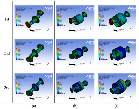
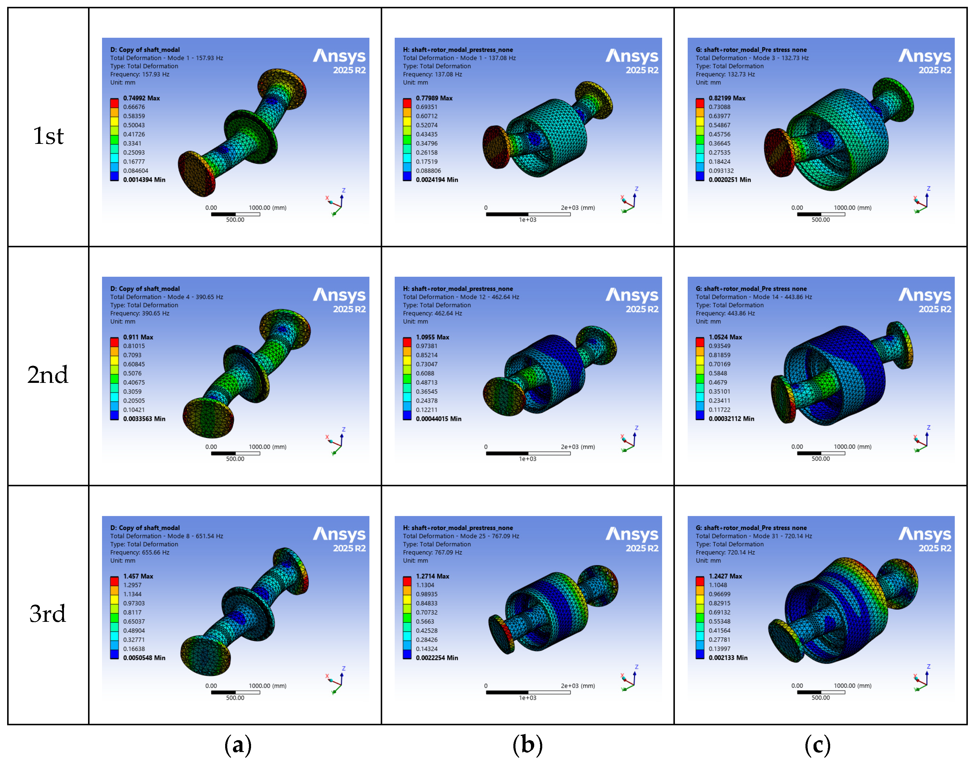
For each model, eigenvalue analysis was performed to obtain the natural frequencies and mode shapes of the dominant lower-order modes. The natural frequencies of each structure calculated from the ANSYS FE model are summarized in Table 5. Bending modes are separated and exhibited in the H direction (horizontal, X-axis) and V direction (vertical, Z-axis) of the rotation axis. The ANSYS Modal analysis results for each target are compared with EMA results in Section 3.3. The corresponding mode shapes of each target are presented in Figure 2.
Table 5.
FEM natural frequency analysis results.
Figure 2.
FEM mode shape analysis by natural frequency order. Rows: 1st, 2nd, and 3rd bending modes. Columns: (a) shaft alone (A); (b) assembly C, shaft + rotor (1); (c) assembly E, shaft + rotor (2).
3.3. Experimental Modal Analysis and FE Model Verification
Experimental modal analysis was performed for the shaft alone (A), reference assembly C, and prediction target assembly E. The purpose of the experiment is to measure the actual natural frequencies and mode shapes of each structure to verify the finite element analysis results and to secure reference data for comparison with substructure coupling-based prediction results. The standard procedure for modal testing based on impact hammer excitation and curve fitting of FRF for mode parameter estimation is described in detail in References [23,24], and this study also constructed the experiment based on this standard procedure.
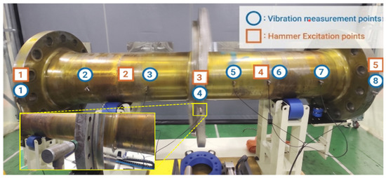
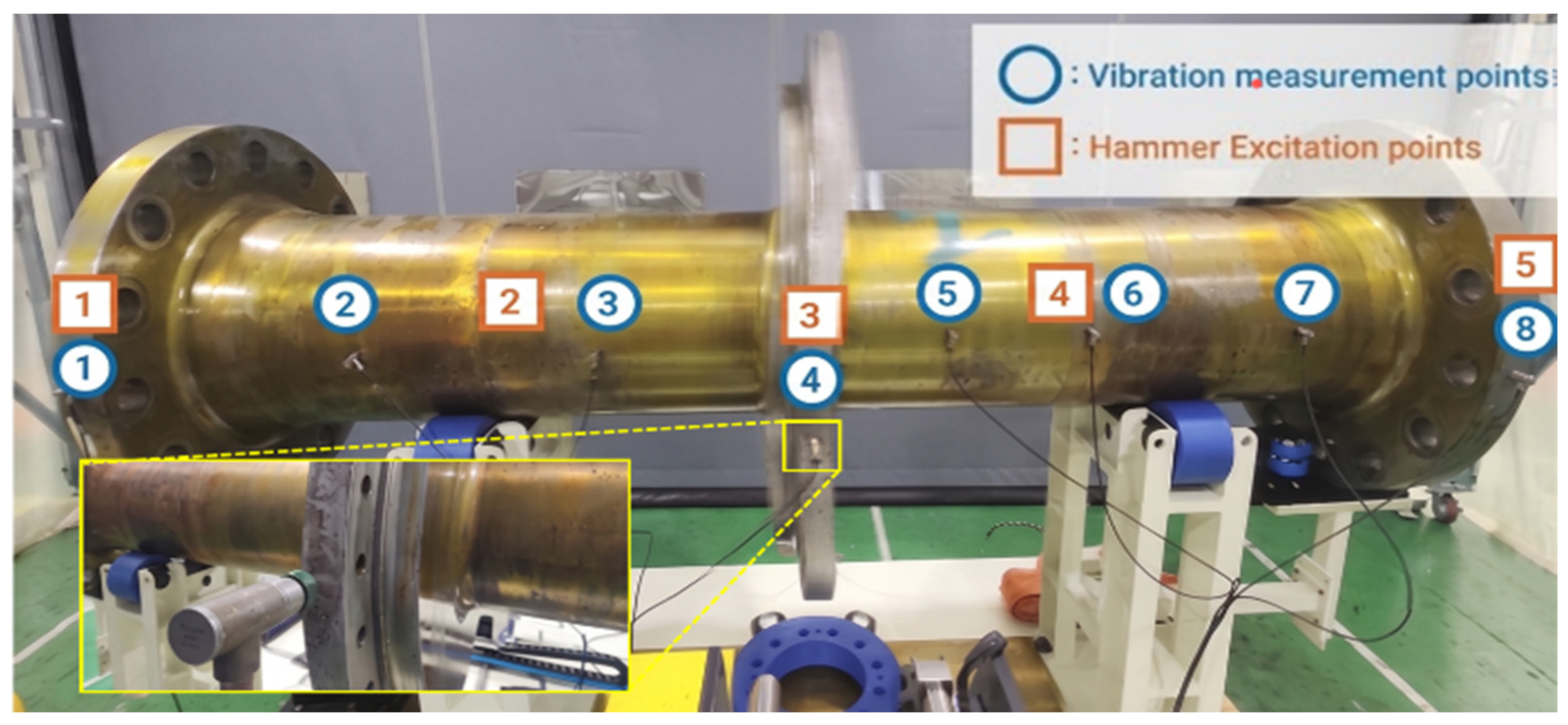
Modal testing was performed through impact hammer excitation and accelerometer-based response measurement. The measurement coordinate system was defined as: horizontal direction (H direction) as the X-axis, vertical direction (V direction) as the Z-axis, and axial direction (A direction) as the Y-axis. Excitation positions were arranged at five locations (L1–L5) along the shaft length direction, and vibration measurement positions consisted of eight locations. H direction and V direction responses were measured simultaneously at each measurement position. The overall measurement configuration and sensor arrangement are shown in Figure 3. The measurement parameters are summarized in Table 6, and the natural frequencies identified from the measured FRFs are summarized in Table 7.
Figure 3.
Experimental modal analysis measurement configuration. Accelerometer positions on the shaft are represented with markers (circle markers: vibration measurement points; square markers: hammer excitation points).
Table 6.
Modal test parameters.
Table 7.
EMA natural frequency measurement results.
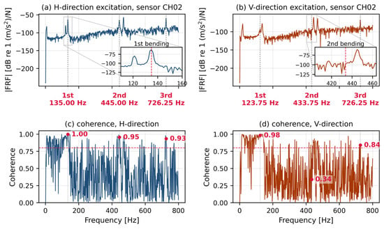
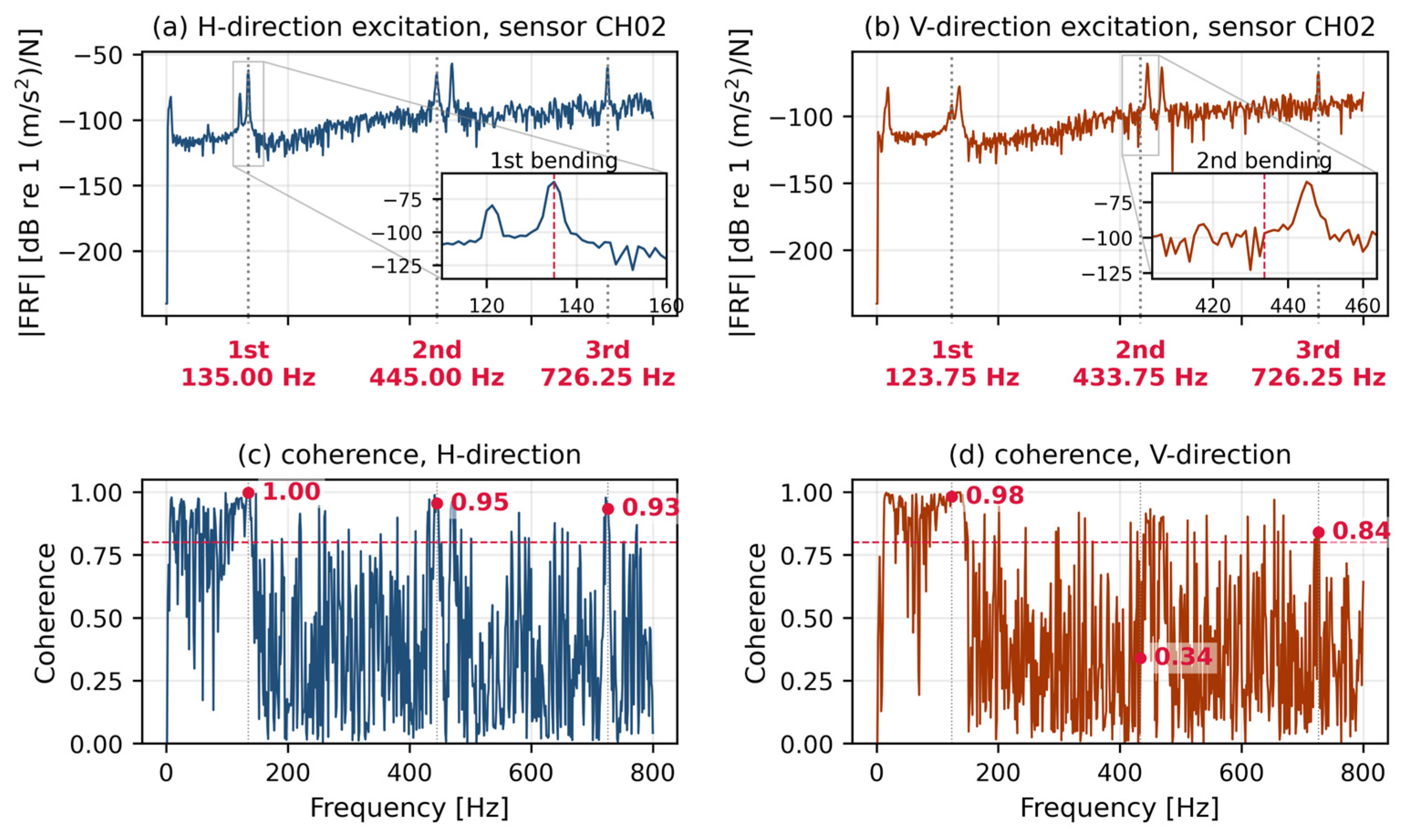
Representative frequency response functions and their coherence are shown in Figure 4 for a single response location under horizontal and vertical excitation. At the second bending mode under horizontal excitation the coherence is 0.95 and the peak is sharply resolved, whereas at the second bending mode under vertical excitation the coherence falls to 0.34 and the peak is broadened. The frequency identified in the latter case is correspondingly less certain.
Figure 4.
Representative frequency response functions and coherence at a single response location. (a) Horizontal excitation, second bending mode. (b) Vertical excitation, second bending mode. (c) coherence, H-direction. (d) coherence, V-direction.
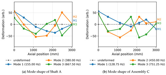
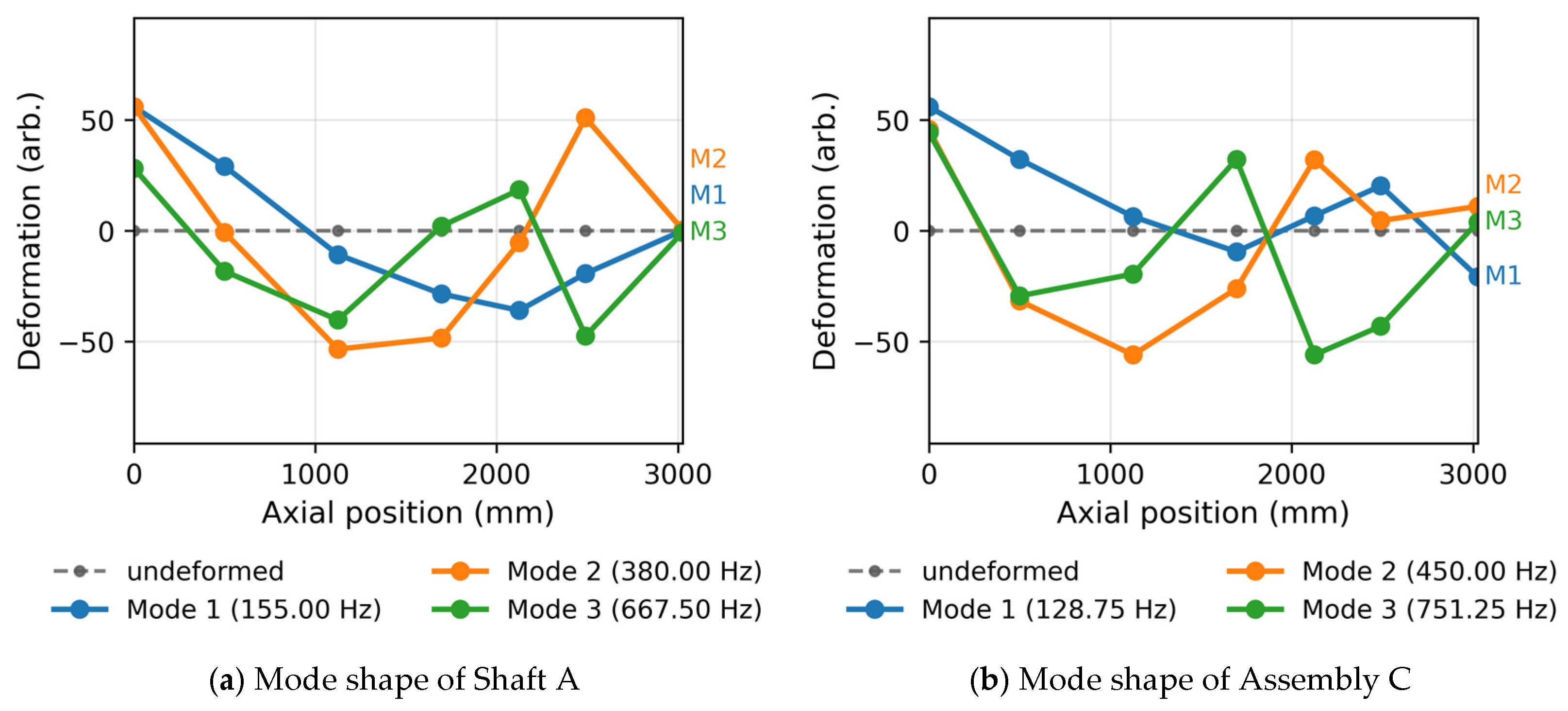
One of the eight response channels was excluded from the analysis. The reduced-order model predicts that location to lie near the antinode of the first bending mode, whereas the measurement recorded a near-zero response there, which is attributed to a measurement failure at that channel. All modal correlation results reported in this paper are, therefore, based on seven response points—the exclusion changes the auto-MAC of the measured set by less than 0.008. The experimental mode shapes reconstructed from these seven response points are presented in Figure 5.
Figure 5.
Representative frequency response functions and coherence at a single response location. (a) Horizontal excitation; the inset zooms on the first bending mode. (b) Vertical excitation; the inset zooms on the second bending mode.
These measurements provide the reference data against which the FE models are assessed in the remainder of this section. Before that comparison is presented, the substructure interface used consistently throughout the study is defined.
The most important element in substructure coupling is the definition of interface DOFs. Interface DOFs are DOFs that satisfy displacement continuity and force equilibrium between the two substructures at the positions where the shaft and rotor are coupled and directly affect prediction accuracy. In this study, the donut-type cross-section at the shaft–rotor coupling (y = −150.0 mm) was selected as the interface region. All X, Y, and Z DOFs of nodes on this surface were defined as boundary DOFs, enabling thorough representation of deformation DOFs in the interface region. This definition is also applied as-is in the Craig–Bampton reduction performed in Section 4.
With the interface thus defined, the remainder of this section presents the first verification stage of this study, whose purpose is to evaluate whether the FE model constructed with ANSYS Workbench sufficiently captures the dynamic characteristics of the actual test specimen. The FE model reliability confirmed in this stage serves as the prerequisite for the Craig–Bampton reduction performed in Section 4 and for the second verification, in which the CB results are compared with ANSYS Modal analysis results.
The comparison results of EMA measurement and ANSYS Modal analysis for the shaft alone (A) are presented in Table 8. For the 1st to 3rd bending modes, H and V directions were compared separately, and the mean absolute error was 2.01%, with a maximum of 2.80%. The corresponding comparisons for the reference assembly C and the prediction target assembly E are given in Table 9 and Table 10, respectively.
Table 8.
Shaft alone (A): EMA vs. ANSYS Modal comparison.
Table 9.
Shaft + rotor (1) assembly (C): EMA vs. ANSYS Modal comparison.
Table 10.
Shaft + rotor (2) assembly (E): EMA vs. ANSYS Modal comparison.
For the shaft + rotor (2) assembly (E), the 1st bending natural frequency appeared at 135.00 Hz in the H direction and 123.75 Hz in the V direction by EMA, and the mean absolute error between the free–free ANSYS Modal analysis and EMA was 2.35%, with the maximum at 7.26% (1st-order V). Overall, the mean absolute error between the ANSYS Modal analysis and EMA for the three targets A, C, and E was 2.70%, with a maximum of 7.26%. Considering the modeling uncertainty of the support condition and the idealization of the fastening conditions, this represents a reasonable level of agreement for an industrial prototype of this scale.
Assembly A and assembly C serve as reference cases within the verification chain, and the prediction target of this study is assembly E.
4. Craig–Bampton-Based Reduced-Order Model Construction and Prediction
This section describes the procedure for constructing Craig–Bampton reduced-order models using matrices extracted from ANSYS in the Python environment. The CB method applied to the reduced-order model is used in Section 5 for the second verification comparing CB with ANSYS Modal and the final verification comparing the CB reduced-order model with EMA measurements.
4.1. Model Construction and Verification Procedure
The overall procedure is summarized in Figure 6. In the offline stage the shaft and the rotor are separated by named selections, their mass and stiffness matrices are extracted independently, and each substructure is reduced on its own. In the online stage the stored models are coupled through a Boolean primal assembly, and the reduced eigenvalue problem is solved. The mass and stiffness matrices of the assembled model are not used at any point in the prediction stage.
Figure 6.
Workflow of the proposed procedure. The offline stage is executed once per substructure and the online stage is repeated for each assembly variant. The mass and stiffness matrices of the assembled model are not used in the prediction stage. Arrows indicate the direction of data flow between stages.
The correctness of the partition is verified directly. The sum of the independently extracted substructure stiffness matrices reproduces the assembled stiffness matrix to a relative error of 4.107 × 10⁻¹⁵, and the mass matrices to 1.945 × 10⁻¹⁶, that is, to machine precision. At the substructure level the reduced models reproduce the corresponding full FE frequencies with a maximum error of 0.064% for the shaft and 0.803% for the rotor, and no negative error occurs in either substructure, as expected for a Ritz reduction at full interface retention.
To perform Craig–Bampton reduction, mass matrices and stiffness matrices constructed with ANSYS Workbench FE models must be extracted. In this study, the system matrices generated during the modal analysis process were brought into the Python environment and processed in sparse matrix format. The mass and stiffness matrices are those of the unconstrained model defined in Section 3.2. No static structural system is linked to the modal system and no prestress is applied, so the matrices used for the reduction are identical to those of the parent finite element model against which the reduced-order model is verified.
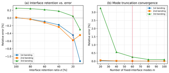
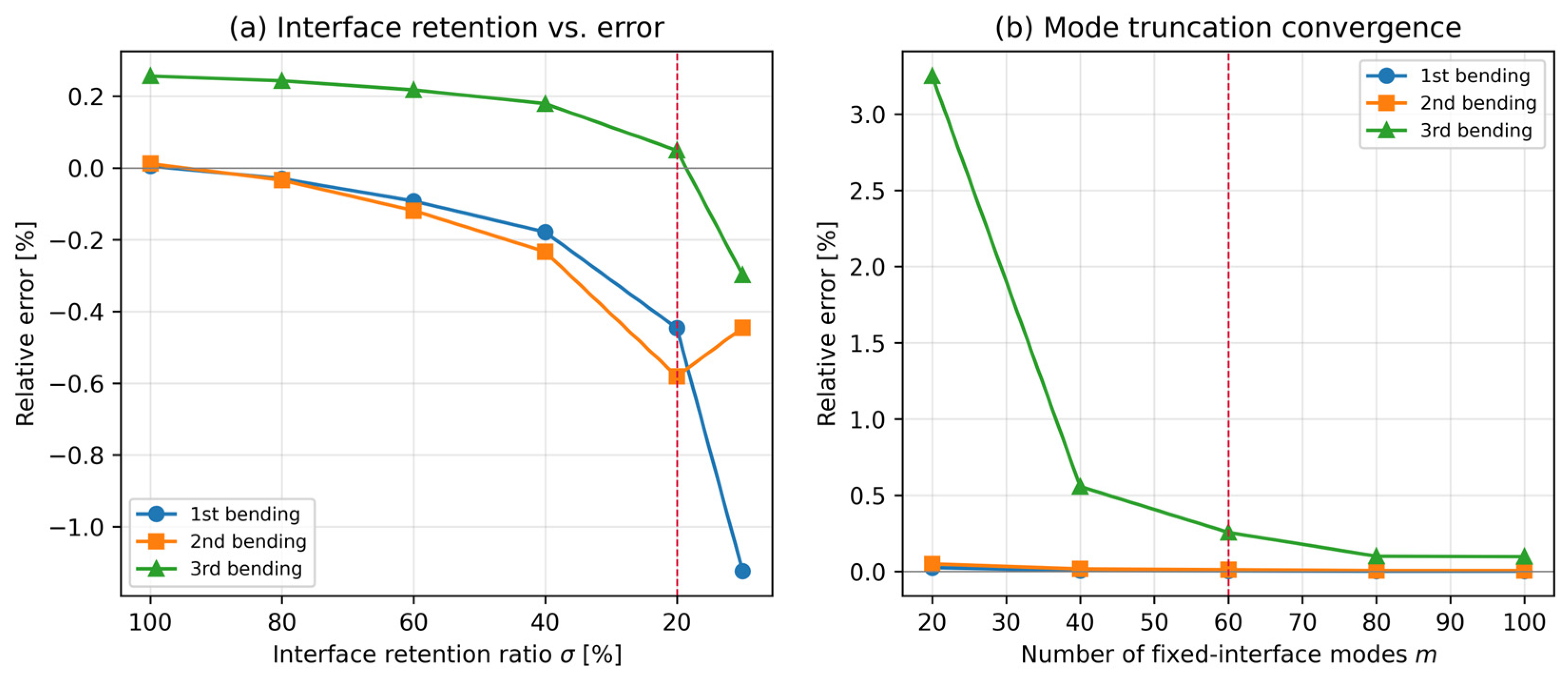
The number of retained fixed-interface normal modes was varied from 20 to 100 while the interface definition and the retention level were held fixed, so that modal truncation is isolated from the interface representation. The results are given in Table 11. The error of the third bending mode decreases from +3.251% at m = 20 to +0.257% at m = 60 and +0.101% at m = 80, while m = 100 gives +0.098%, and convergence is, therefore, essentially complete at m of about 80. The error of the first bending mode remains below 0.026% and that of the second below 0.05% throughout.
Table 11.
Convergence with the number of retained fixed-interface normal modes (full interface retention).
A value of m = 60 is adopted in this study. The cost of the online eigenvalue problem scales with m, and it is the online stage that is repeated for every design variant; in addition, the residual error of 0.26% at m = 60 is an order of magnitude smaller than the uncertainty of the modal test against which the model is validated.
During the calculation of fixed-interface modes, since the number of DOFs is very large, the shift-invert technique is applied to partially extract only lower-order natural modes near the frequency range of interest [25,26]. Constraint modes are calculated as the static responses when unit displacement is applied to each interface DOF (NS_BI, donut-type cross-section of shaft–rotor coupling), with the remaining DOFs fixed, and are generated by the relationship in Equation (6). For the shaft (A) model in this study, X, Y, and Z DOFs of interface region nodes are defined as boundary DOFs (5259 boundary DOFs at 1753 interface nodes), and constraint modes are accordingly configured in the same number. During calculation, the inverse matrix is not directly obtained but LU decomposition is performed only once, after which the static responses to unit displacements for each interface DOF are repetitively calculated to secure numerical stability and computational efficiency [27].
Through the above process, Craig–Bampton transformation is applied to each substructure according to Equations (4)–(10) to generate the reduced mass matrix MCB and stiffness matrix KCB. Through this transformation, interior DOFs are replaced by a small number of mode coordinates and the total number of DOFs decreases significantly.
4.2. Reduced DOF Information
When the CB pipeline is applied to assembly E, the model is reduced from 192,678 degrees of freedom to 5379 at full interface retention and to 1173 at the recommended retention level of 20%, corresponding to reduction ratios of 97.21% and 99.39%, respectively. The interface comprises 5259 degrees of freedom at 1753 nodes.
Measured computational cost is reported in Table 12. A full finite element modal analysis of assembly E requires 28.4 s and 2125 MB. The offline construction of the reduced-order models requires 245 s for the shaft and 167 s for the rotor. The online stage requires 4.87 s and 522 MB at full interface retention and 0.151 s at the recommended retention level. The online stage is, therefore, faster than a full analysis while using about one quarter of the memory, and the offline stage is paid once per component. Any figure derived from complexity scaling is a theoretical estimate rather than a measured speedup, and such estimates are not used here.
Table 12.
Measured computational cost. AMD Ryzen Threadripper PRO 7985WX (64 cores, 3.20 GHz), 1.00 TB RAM.
All timings were measured on a workstation with an AMD Ryzen Threadripper PRO 7985WX processor (64 cores, 3.20 GHz) and 1.00 TB of RAM, running the full finite element analysis in ANSYS Workbench 2025 R2 and the reduced-order pipeline in Python with sparse solvers. The DOF scale before and after reduction for A, C, and E assemblies is summarized in Table 13.
Table 13.
CB reduction DOF comparison.
5. Results and Discussion
This section quantitatively evaluates the accuracy of the substructure coupling-based prediction procedure proposed in this study by comparing the results of the Craig–Bampton reduced-order model constructed in Section 4 with ANSYS Modal analysis values and EMA measurements. This section conducts the second verification, the comparison of the CB reduced-order model with ANSYS Modal analysis results, and evaluates the prediction accuracy against measurement through the final verification comparing the CB reduced-order model with EMA measurements.
5.1. Verification Method
The verification framework of this study is defined as shown in Table 14. Since A is a single substructure, all three results of EMA, ANSYS, and CB can be directly compared at the single substructure level, and C and E compare the same three results at the assembly level as coupled results of two substructures. This three-stage verification structure validates the accuracy of the reduction procedure at both the single substructure level and the assembly level.
Table 14.
Verification matrix of this study.
5.2. CB Reduced-Order Model Analysis Results
The accuracy of the shaft reduced-order model at the substructure level is reported in Section 4.1, where the reduction reproduces the parent finite element frequencies to within 0.064%. Assembly A, therefore, serves as a reference case for the FE-to-EMA stage of the verification chain, and the reduction results discussed below concern assemblies C and E.
Assembly C serves as a reference case for the finite element stage of the verification chain, where it is compared against the measurements in Section 3.3. The prediction target of this study is assembly E, and the accuracy of the reduction is, therefore, assessed on that assembly. The shaft and rotor reduced-order models are coupled through the Boolean primal assembly described in Section 4.1, so that the mass and stiffness matrices of the assembled model are not used at any point. The coupled model comprises 5379 degrees of freedom. The comparison with the ANSYS modal results is presented in Table 15.
Table 15.
Assembly E: CB vs. ANSYS Modal comparison.
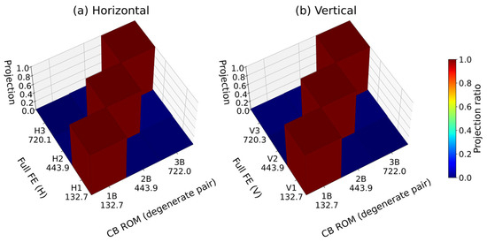
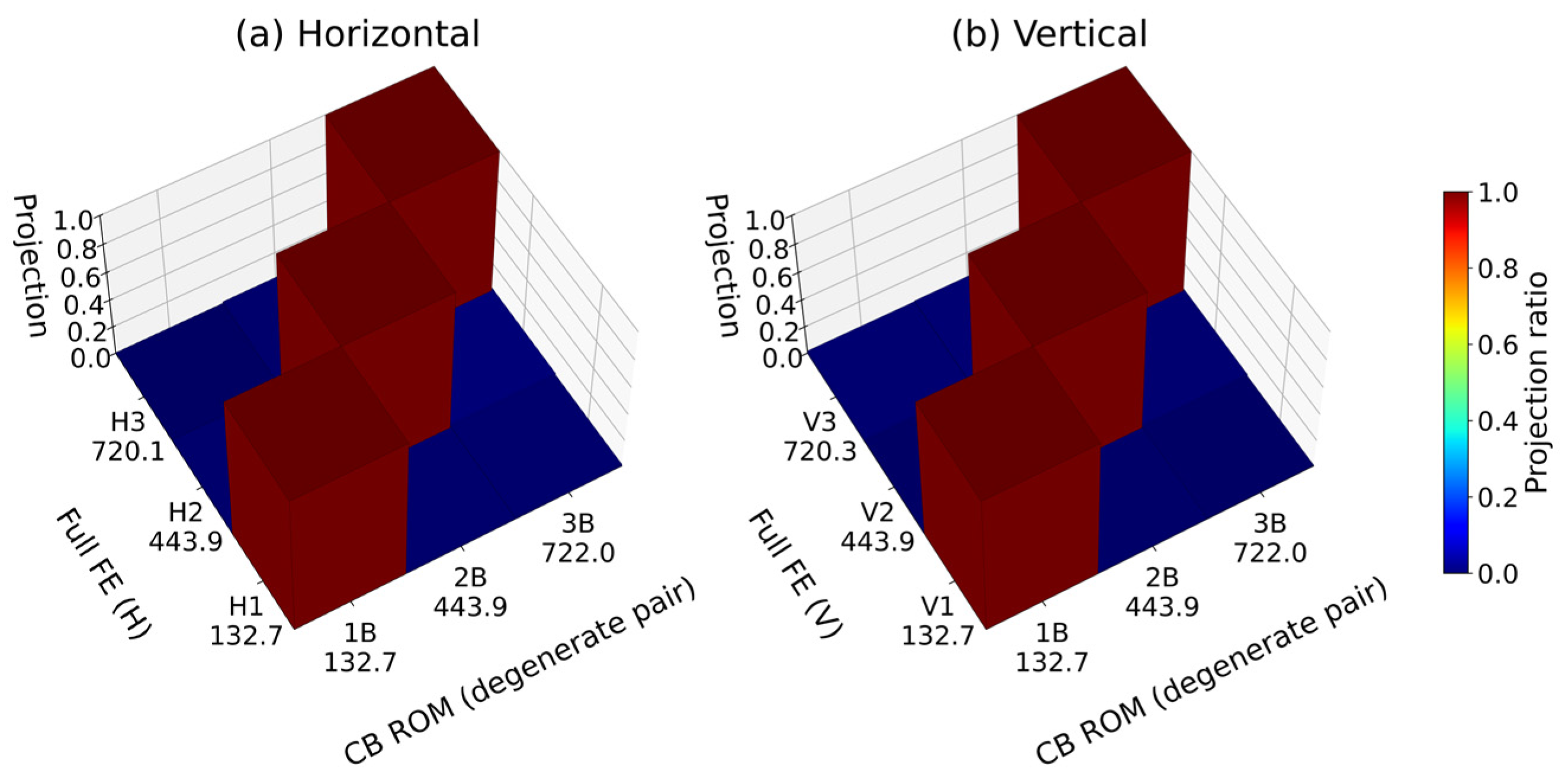
The CB reduced-order model of assembly E yielded a mean absolute error of 0.087% compared with the reference ANSYS modal analysis, with a maximum of 0.257% in the third bending mode. The first and second bending modes agree to within 0.012% in both directions. The horizontal and vertical CB values coincide because the unconstrained axisymmetric assembly yields a degenerate bending pair, as discussed above.
Because the assembly is axisymmetric and the models are unconstrained, the bending modes appear as repeated eigenvalues in both the full finite element model and the reduced-order model. For a repeated pair, the orientation of each eigenvector within the corresponding plane is not unique, so mode-by-mode MAC values [28] for such a pair split toward 0.5 and reflect the choice of basis rather than the agreement of the mode shapes. Increasing the number of retained fixed-interface modes does not alter this, since the degeneracy originates from the boundary condition rather than from modal truncation.
The correlation between the two-dimensional subspaces spanned by each degenerate pair, evaluated from the principal angles, is, therefore, reported in Figure 7. For a non-degenerate mode, the subspace measure reduces to the conventional MAC, so a single definition applies across the whole frequency range.
Figure 7.
Modal correlation between the reduced-order model and the full FE model for the bending modes. (a) Horizontal direction. (b) Vertical direction.
The first three bending pairs are compared in Table 16. Every mode group below 720 Hz gives a subspace MAC of 1.0000, and the mean over the range up to 1000 Hz is 0.995. No rank deficiency occurs, that is, the reduced-order model does not collapse any degenerate pair into a single mode, and no reduced-order mode is left unmatched. The lowest value over the full range, 0.886, occurs above 900 Hz, outside the frequency range of interest, and is consistent with the truncation behavior discussed in Section 4.1.
Table 16.
Reduced-order model versus full FE model, bending modes.
5.3. Prediction Accuracy Evaluation
This section evaluates the final prediction accuracy of this study. The natural frequencies of assembly E from the CB reduced-order model are directly compared with EMA measurements to evaluate how accurately the proposed procedure predicts the dynamic characteristics of the actual test specimen. The comparison results are presented in Table 17.
Table 17.
Assembly E prediction: CB vs. EMA comparison.
Excluding the 1st vertical mode, the mean absolute error over the remaining five modes is 1.28%, with a maximum of 2.34%. The 1st horizontal mode agrees to within 1.68% and the 3rd bending modes to within 0.59% in both directions, showing that the CB pipeline reproduces the measured bending frequencies to within 2.34% over these modes. The deviation of the 1st vertical mode is examined in Section 5.4.
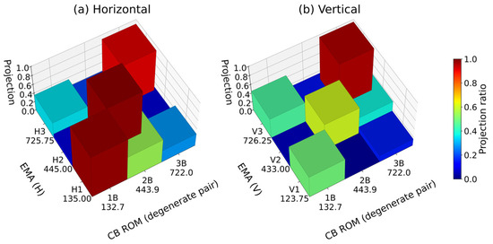
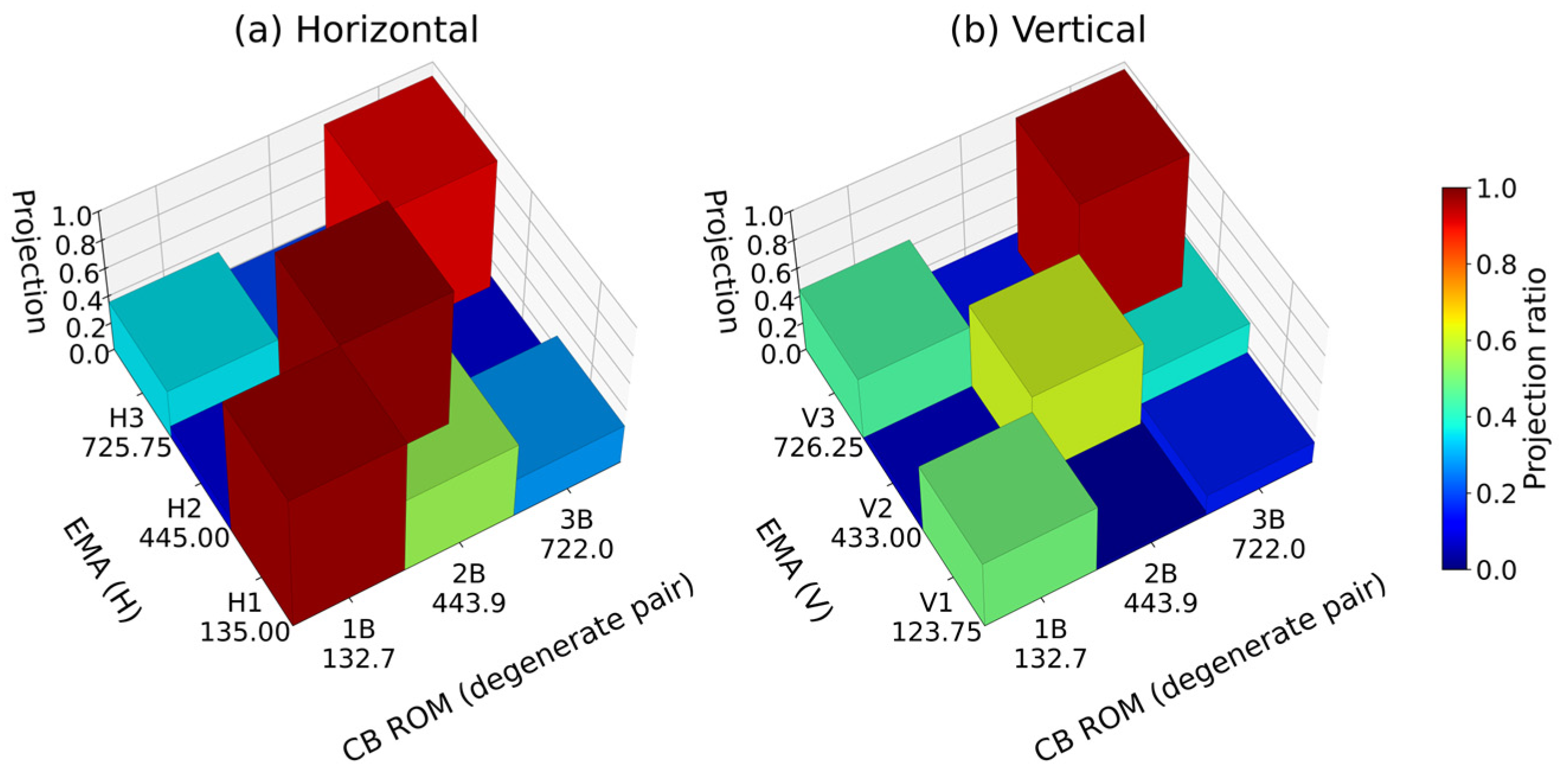
The same subspace measure is applied to the comparison with the measurements, and the results are given in Figure 8 and Table 18. The first bending pair gives 0.979 and 0.916, the second horizontal mode 0.989, and the third vertical mode 0.981, against a random-alignment baseline of 0.286 for seven response points.
Figure 8.
Modal correlation between the reduced-order model and the experimental modal analysis for the bending modes. (a) Horizontal direction. (b) Vertical direction. Seven valid response points.
Table 18.
Reduced-order model versus experimental modal analysis. Seven valid response points.
5.4. Quantitative Separation of the FE Model Stage Error
A relatively large error of 7.26% is observed between the CB predicted value (132.74 Hz) and the EMA measured value (123.75 Hz) for the 1st V mode of assembly E. In this section, the source of this error is quantitatively diagnosed using the verification chain structure of this study. Table 19 summarizes the errors of three comparison pairs for the same mode.
Table 19.
Assembly E 1st V mode: error source separation analysis.
The results in Table 19 show that the 7.26% error in the 1st V mode originates entirely from the FE model stage. The difference between the CB reduced-order model and the ANSYS Modal analysis is 0.002%, confirming that the reduction procedure itself introduces no appreciable error. The error between the ANSYS Modal analysis and the EMA measurement already reaches 7.26%, and the same discrepancy is propagated to the CB prediction, and the cause lies in the representation of the support condition. The models used for the reduction are unconstrained, so the axisymmetric assembly yields a degenerate bending pair and no directional separation can arise, whereas the modal tests were conducted with the shaft resting on two rollers. Because the rollers act over a limited part of the circumference, they break the axisymmetry of the structure and constrain vertical and horizontal bending with different effectiveness. This is corroborated by the mode shapes: the measured first horizontal and first vertical modes are only weakly correlated with each other, so frequency separation and shape difference point to the same origin. The equivalent stiffness and contact extent of the roller supports are accordingly identified as the leading candidates for model updating, followed by the equivalent rotational stiffness of the flange connection, the equivalent elastic modulus of the laminated rotor core, the equivalent mass and inertia of attached components, and the compliance of the foundation. This FE model stage error can be improved through correction of bearing and fastening part stiffness via model updating techniques [29], and related research on uncertainty propagation in substructure coupling procedures has also been reported [30]. Such analysis is possible precisely because this study’s verification chain is separated into three stages of verification (FE analysis and EMA comparison, CB reduced-order model and FEM comparison, and CB reduced-order model and EMA comparison).
It is worth noting that the measured horizontal and vertical modes, although weakly correlated with each other, both project strongly onto the same subspace of the reduced-order model—two mutually orthogonal vectors can lie within one plane. The model, therefore, reproduces the plane of deformation correctly, while the orientation selected within that plane is governed by the support condition that the unconstrained model does not represent. The deviation is thus localized to the support representation rather than distributed across the reduction.
5.5. Interface DOF Representation Level and Reduction Ratio at Shaft–Rotor Interface
This section quantitatively analyzes the effect of the number of interface DOFs at the shaft–rotor interface on the accuracy of the reduced-order model and quantifies the resulting error-retention relation for the annular shaft–rotor interface examined here. The interface retention ratio is defined as σ = nb*/nb = rank(R)/nb, where R is the selection matrix of Equation (12), and it is varied stepwise from 100% to 10% for assembly E. At each setting the selection matrix R is rebuilt, the repartition of Equations (13) and (14) is applied, and the constraint modes and fixed-interface normal modes are recomputed from Equations (6) and (7) before the two reduced-order models are coupled through Equations (15) and (16). No quantity is carried over between retention levels. The ANSYS Modal comparison errors of the 1st, 2nd, and 3rd bending modes and the total reduction rate are then compared. The number of fixed-interface normal modes is fixed at 60.
The rows of R are selected from the geometry of the axisymmetric interface surface. Each interface node is assigned to a radial coordinate, and the nodes are grouped into rings of constant (y, r), so that a ring collects the nodes that differ only in circumferential position, as defined in Equation (17):
This grouping covers both parts of the spigot joint: on the annular flange face the rings are formed at constant y over successive radii, and on the in-row cylindrical surface at constant r over successive axial positions. Within each ring the retained nodes are drawn at uniform spacing in the circumferential coordinate, and their number is:
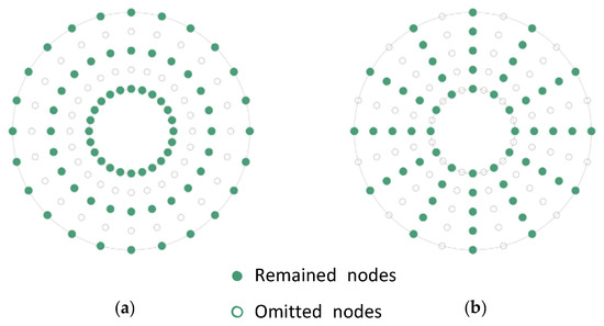
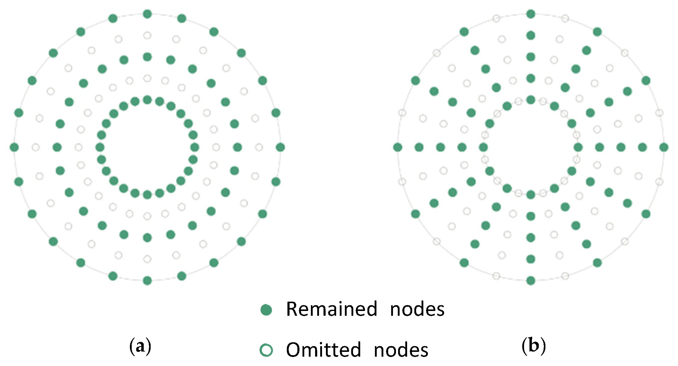
where Nj is the number of nodes in ring Gj. The floor of four nodes per ring is the sampling bound derived later in this section. The selection matrix R is then the indicator matrix of the retained set, formed as the union of the retained nodes over all rings, and the released nodes populate the complementary selection Rc of Equation (13). Every ring is, therefore, preserved, and the thinning acts only in the circumferential direction, which is scheme (b) of Figure 9. Scheme (a), in which entire rings are omitted, was not used because it removes the circumferential resolution on which the bending deformation depends.
Figure 9.
Interface node sampling schemes at the annular coupling cross-section. (a) Ring-wise omission: each retained ring is fully sampled and other rings are omitted (not adopted). (b) Radially aligned, circumferentially uniform sampling: nodes are retained at uniform angular spacing on every ring across all radii (adopted in this study).
These observations can be explained by the circumferential harmonic content of the interface displacement field. For the bending modes of interest, the annular cross-section deforms in a single circumferential harmonic: one side rises while the opposite side descends, so the field completes one cosine period around the circumference, corresponding to a circumferential order of n = 1. Such a field is represented without aliasing when the number of retained nodes per ring satisfies , by the same reasoning as the Nyquist criterion. Four nodes per ring are, therefore, sufficient in principle, and the retention levels examined in Table 20 remain well above this bound. The bound, therefore, constrains the row selection of R in Equation (12) rather than its rank alone: it is valid only when the retained rows are distributed at uniform circumferential spacing within every ring, which is what Equation (18) enforces.
Table 20.
Assembly E: reduction ratio (%) and mode-specific relative error for each interface DOF ratio σ (%).
The criterion is expressed in nodes per ring rather than as a fraction of the total interface degrees of freedom, and in this form it is independent of mesh density and interface diameter. Its validity is restricted to interfaces that admit a circumferential parameterization, that is, to axisymmetric annular interfaces. Because the retained nodes are thinned at uniform angular spacing, the rotational symmetry is preserved, and the horizontal and vertical bending modes are affected to the same degree at every retention level.
Two approximations act in opposite directions. Reducing the number of retained interface nodes enlarges the null space of the projector Pb in Equation (12), so the compatibility of Equation (15) is imposed on fewer degrees of freedom—the coupled model softens and the predicted frequencies fall. The first bending error decreases monotonically from +0.005% at full retention to −0.447% at 20% and −1.124% at 10%. Truncation of the fixed-interface normal modes acts in the opposite sense and accounts for the +0.257% error of the third bending mode at full retention. The near-zero third-mode error of +0.049% at 20% retention is the result of these contributions cancelling and should not be read as an improvement in accuracy.
Because the first bending mode deviates monotonically and the deviation of all three modes remains bounded, the error-retention relation in Table 20, plotted in Figure 10, allows a retention level to be selected against a stated error tolerance for this interface. For the present assembly, a retention level of 20% gives the first three bending modes predicted within 0.60%, the reduced interface comprises 1053 of 5259 degrees of freedom, and the assembled reduced model decreases from 5379 to 1173 degrees of freedom, a reduction of 99.39% relative to the parent model. The online coupling and eigenanalysis time fall accordingly from 4.87 s to 0.151 s, a factor of 32.3, as reported in Section 4.2. At 10% retention, the first bending mode degrades to −1.12%.
Figure 10.
(a) Relative error of the first three bending modes versus the interface retention ratio. (b) Convergence with the number of retained fixed-interface normal modes.
The findings of this section apply to axisymmetric shaft–rotor assemblies under stationary modal conditions, that is, to annular interfaces analyzed without gyroscopic effects, spin softening, or speed-dependent bearing behavior. For general asymmetric couplings, interface DOF reduction may have different effects on reduction accuracy. They are further restricted to the single annular interface, mesh, and mode range examined here. The argument that the four-node-per-ring bound is independent of mesh density follows from the circumferential sampling condition and has not been verified against an independent discretization, and variations in rotor configuration, support condition, and sampling scheme likewise remain untested.
5.6. Scope and Limitations
The results reported above were obtained from a single industrial prototype and a single interface geometry. This section states the conditions under which they were obtained and the extent to which they may be expected to transfer, considering in turn the structural characteristics of the assembly examined, the topology of the interface, and the scope of the present validation, so that the numerical capability demonstrated here is not read as a general engineering claim.
The structural characteristics of the assembly examined bound the result in the first instance. The two rotors considered differ in mass and inertia, approximately 3.1 t and 3.5 t, but share the same coupling geometry, and the modes of interest are the first three global bending modes of the assembly. The interface displacement field associated with these modes is dominated by a single circumferential harmonic, and this property is what the sampling criterion of Equation (18) relies upon. Assemblies whose stiffness distribution differs substantially between variants, or in which local component modes contribute to the frequency range of interest, do not satisfy this condition—the retention levels reported here should not be transferred to such cases without re-evaluation.
The topology of the interface bounds it further. The coupling examined is a single annular spigot joint, discretized with one mesh and thinned by one sampling scheme. The criterion is defined only for interfaces that admit a circumferential parameterization. For non-axisymmetric couplings, for assemblies containing several interfaces, and for joints represented by discrete bolt connections rather than a continuous bonded surface, neither the sampling rule of Equation (18) nor the retention levels of Table 20 apply as stated. The independence of the four-node-per-ring bound from mesh density follows from the sampling argument and has not been verified against an independent discretization.
The scope of the present validation should also be stated plainly. It rests on one industrial prototype, two assemblies, five identified modes below 720 Hz, and stationary modal conditions. The tests were conducted as a deterministic verification procedure—repeated builds and instrumentation campaigns, which would be required for a statistical quantification of uncertainty, lie outside the scope of this work. The accuracy figures reported here, therefore, characterize the present configuration and are not offered as a general performance specification for the method.
The scope of this study is bounded by three modeling conditions. First, the models used for the reduction are unconstrained, so gravity-induced stress stiffening and the elastic support of the test rig are not represented. Since the self-weight stress state of the shaft depends on the rotor mounted on it, a substructure model including such effects would be valid only for one assembly, which is incompatible with the rotor-replacement reuse addressed here. This does not imply that prestressed substructure models are invalid in general, only that their applicability is restricted to the state for which they were built. Second, the analysis is limited to stationary modal conditions, so gyroscopic effects, spin softening, and speed-dependent bearing behavior are not represented. Third, the shaft meshes of assemblies C and E are non-conforming, so the reuse of a shaft reduced-order model across assemblies could not be demonstrated. The present validation is restricted to the accuracy of partition-independent reduction and coupling.
The flange interface is modeled by shared topology, so the two bodies share nodes at the mating surface and are fully bonded. High-tension bolt preload establishes contact pressure over the faces, and under the small-amplitude excitation of modal testing the interface remains adhered without opening or slip, so this representation is appropriate for the present analysis. Contact nonlinearity would have to be considered for large-amplitude or transient loading.
6. Conclusions
This study applied the Craig–Bampton substructure coupling method to predict changes in natural frequencies upon rotor replacement in a shaft generator shaft–rotor assembly and verified its accuracy through a three-stage verification framework consisting of comparisons between FE analysis and EMA measurements, between the CB reduced-order model and FEM results, and between the CB reduced-order model and EMA measurements.
The framework reduced assembly E from 192,678 degrees of freedom to 5379 at full interface retention, a reduction of 97.21%. For the prediction target assembly E, the reduced-order model reproduced the parent finite element model to within 0.012% for the first two bending modes and 0.257% for the third, with a subspace MAC of 1.0000 for every mode group below 720 Hz, directly verifying that the reduction procedure introduces virtually no additional error beyond what is already present in the finite element model. When the natural frequencies of assembly E computed from the reduced-order model were compared with the EMA measurements, a mean absolute error of 1.28% was obtained over five modes, an accuracy consistent with the tolerance normally applied at the early design-review stage for this class of assembly.
Because the CB reduced-order model agreed with the ANSYS modal results to within 0.002% for the same mode, the 7.26% discrepancy between the ANSYS modal analysis and the EMA measurement was identified as the dominant source of error. This separation of error origins, made possible by the layered verification structure, provides direct guidance on where model updating efforts should be focused in future work.
In the interface sensitivity study, the first three bending modes were predicted within 0.60% at a retention level of 20%, and the reduction ratio increased from 97.21% at full interface retention to 99.39%. The assembled reduced model decreased from 5379 to 1173 degrees of freedom, and the online coupling and eigenanalysis time fell from 4.87 s to 0.151 s, a factor of 32.3. Because the first bending mode error varies monotonically with the retention level and the deviation of all three modes remains bounded, the error-retention relation can be used to select a retention level for annular interfaces of the type examined.
Taken together, these results show that, for the assembly examined, the Craig–Bampton procedure predicts the bending natural frequencies after rotor replacement without a full re-analysis, at an online cost of 0.151 s against 28.4 s for the full finite element model. Whether this capability extends to routine early-stage dynamic-characteristic review of shaft generators, in which customer shafting conditions are determined in a stepwise manner, depends on the structural characteristics and interface topology of the individual product and would require validation on configurations beyond the one studied here. Future work will pursue expansion to experiment-based substructure coupling using the transmission simulator concept, and the representation of the roller support stiffness and contact extent through model updating techniques [29].
Author Contributions
Conceptualization, J.S. and S.B.; methodology, J.S. and S.B.; software, J.S.; validation, J.S. and S.B.; formal analysis, J.S.; investigation, J.S.; resources, J.S. and S.B.; data curation, J.S.; writing—original draft preparation, J.S.; writing—review and editing, J.S. and S.B.; visualization, J.S.; supervision, S.B.; project administration, S.B. All authors have read and agreed to the published version of the manuscript.
Funding
This work was supported by the National Research Foundation of Korea (NRF) grant funded by the Korea government (MSIT) (No.RS-2024-00341872).
Data Availability Statement
The data supporting the findings of this study are available from the corresponding author upon reasonable request. The data are not publicly available because they contain proprietary and commercially sensitive information related to the industrial prototype investigated in this study.
Acknowledgments
The authors gratefully acknowledge the technical assistance provided during the preparation and experimental modal testing of the shaft generator prototype.
Conflicts of Interest
J.S. is an employee of HD Hyundai Electric Co., Ltd., the manufacturer of the prototype investigated in this study. The company had no role in the design of the study, in the collection, analysis or interpretation of the data, or in the decision to publish the results. The authors declare no other conflicts of interest.
Abbreviations
The following abbreviations are used in this manuscript:
| Abbreviations | |
| CB | Craig–Bampton |
| DOF | Degree of freedom |
| EMA | Experimental modal analysis |
| FE/FEM | Finite element/finite element model |
| FRF | Frequency response function |
| H | Horizontal direction (X-axis) |
| MAC | Modal assurance criterion |
| ROM | Reduced-order model |
| TS | Transmission simulator |
| V | Vertical direction (Z-axis) |
| Nomenclature | |
| A, B, C, D, E | Substructure/assembly symbols (see Table 1) |
| K | Stiffness matrix |
| KCB | Reduced stiffness matrix (Craig–Bampton) |
| M | Mass matrix |
| MCB | Reduced mass matrix (Craig–Bampton) |
| nb | Number of boundary DOFs |
| ncb | Total reduced DOFs (n_b + fixed-interface modes) |
| qk | Generalized coordinates for selected modes |
| TCB | Craig–Bampton transformation matrix |
| xb | Boundary DOF vector |
| xi | Interior DOF vector |
| Φik | Fixed-interface normal mode matrix |
| Ψib | Constraint mode matrix |
| Λk | Diagonal matrix of fixed-interface natural frequency squares |
| σ | Interface DOF retention ratio (%) |
References
- Lalanne, M.; Ferraris, G. Rotordynamics Prediction in Engineering, 2nd ed.; John Wiley & Sons: Chichester, UK, 1998. [Google Scholar]
- de Klerk, D.; Rixen, D.J.; Voormeeren, S.N. General framework for dynamic substructuring: History, review, and classification of techniques. AIAA J. 2008, 46, 1169–1181. [Google Scholar] [CrossRef] [Scilit]
- Allen, M.S.; Rixen, D.; van der Seijs, M.; Tiso, P.; Abrahamsson, T.; Mayes, R.L. Substructuring in Engineering Dynamics: Emerging Numerical and Experimental Techniques; CISM International Centre for Mechanical Sciences; Springer: Cham, Switzerland, 2020; Volume 594. [Google Scholar]
- Craig, R.R., Jr.; Bampton, M.C.C. Coupling of substructures for dynamic analyses. AIAA J. 1968, 6, 1313–1319. [Google Scholar] [CrossRef] [Scilit]
- Roettgen, D.; Seeger, B.; Tai, W.C.; Baek, S.; Dossogne, T.; Allen, M.; Kuether, R.; Brake, M.R.W.; Mayes, R. A comparison of reduced order modeling techniques used in dynamic substructuring. In Proceedings of the 33rd International Modal Analysis Conference (IMAC XXXIII), Orlando, FL, USA, 2–5 February 2015. [Google Scholar]
- Jin, H.G.; Lee, B.; Baek, S. Development of a force identification method using component mode synthesis and system-level response. Trans. Korean Soc. Noise Vib. Eng. 2025, 35, 108–120. [Google Scholar] [CrossRef] [Scilit]
- Allen, M.; Mayes, R.; Bergman, E. Experimental modal substructuring to couple and uncouple substructures with flexible fixtures and multi-point connections. J. Sound Vib. 2010, 329, 4891–4906. [Google Scholar] [CrossRef] [Scilit]
- Allen, M.S.; Mayes, R.L. Comparison of FRF and modal methods for combining experimental and analytical substructures. In Proceedings of the 25th International Modal Analysis Conference (IMAC XXV), Orlando, FL, USA, 19–22 February 2007. [Google Scholar]
- Mayes, R. A Craig-Bampton experimental dynamics substructure using the transmission simulator method. In Proceedings of the 33rd International Modal Analysis Conference (IMAC XXXIII), Orlando, FL, USA, 2–5 February 2015. [Google Scholar]
- Balmès, E. Use of generalized interface degrees of freedom in component mode synthesis. In Proceedings of the 14th International Modal Analysis Conference (IMAC XIV), Dearborn, MI, USA, 12–15 February 1996. [Google Scholar]
- Castanier, M.P.; Tan, Y.-C.; Pierre, C. Characteristic constraint modes for component mode synthesis. AIAA J. 2001, 39, 1182–1187. [Google Scholar] [CrossRef] [Scilit]
- Lindberg, E.; Hörlin, N.-E.; Göransson, P. Component mode synthesis using undeformed interface coupling modes to connect soft and stiff substructures. Shock Vib. 2013, 20, 157–170. [Google Scholar] [CrossRef]
- Carassale, L.; Maurici, M. Interface reduction in Craig-Bampton component mode synthesis by orthogonal polynomial series. J. Eng. Gas Turbines Power 2018, 140, 052504. [Google Scholar] [CrossRef] [Scilit]
- Schwerdt, L.; Panning-von Scheidt, L.; Wallaschek, J. A priori interface reduction for substructuring of multistage bladed disks. In Dynamic Substructures, Volume 4; Conference Proceedings of the Society for Experimental Mechanics Series; Springer: Cham, Switzerland, 2020; pp. 13–21. [Google Scholar]
- Paehr, M.; Panning-von Scheidt, L. Application of interface reduction methods to rotordynamic casing models. J. Eng. Gas Turbines Power 2025, 147, 051019. [Google Scholar] [CrossRef] [Scilit]
- Shanmugam, A.; Padmanabhan, C. A fixed-free interface component mode synthesis method for rotordynamic analysis. J. Sound Vib. 2006, 297, 664–679. [Google Scholar] [CrossRef] [Scilit]
- Wagner, M.B.; Younan, A.; Allaire, P.; Cogill, R. Model reduction methods for rotor dynamic analysis: A survey and review. Int. J. Rotating Mach. 2010, 2010, 273716. [Google Scholar] [CrossRef] [Scilit]
- Förster, A.; Panning-von Scheidt, L. Interface reduction in an equivalent linearization algorithm for nonlinearly coupled systems under random excitation. In Proceedings of the ASME Turbo Expo 2022, Rotterdam, The Netherlands, 13–17 June 2022. [Google Scholar]
- Tran, D.-M. Component mode synthesis methods using partial interface modes: Application to tuned and mistuned structures with cyclic symmetry. Comput. Struct. 2009, 87, 1141–1153. [Google Scholar] [CrossRef] [Scilit]
- Bui, T.A.; Kim, J.-S.; Park, J. Virtual beam-based prior interface reduction for optimizing plate substructures with complex interface geometry. Arch. Appl. Mech. 2025, 95, 164. [Google Scholar] [CrossRef] [Scilit]
- Rixen, D.J. A dual Craig-Bampton method for dynamic substructuring. J. Comput. Appl. Math. 2004, 168, 383–391. [Google Scholar] [CrossRef] [Scilit]
- Craig, R.R.; Kurdila, A. Fundamentals of Structural Dynamics, 2nd ed.; John Wiley & Sons: Hoboken, NJ, USA, 2006. [Google Scholar]
- Ewins, D.J. Modal Testing: Theory, Practice and Application, 2nd ed.; Research Studies Press: Baldock, UK, 2000. [Google Scholar]
- Heylen, W.; Lammens, S.; Sas, P. Modal Analysis Theory and Testing; Katholieke Universiteit Leuven: Leuven, Belgium, 1997. [Google Scholar]
- Lehoucq, R.B.; Sorensen, D.C.; Yang, C. ARPACK Users’ Guide: Solution of Large-Scale Eigenvalue Problems with Implicitly Restarted Arnoldi Methods; SIAM: Philadelphia, PA, USA, 1998. [Google Scholar]
- Golub, G.H.; Van Loan, C.F. Matrix Computations, 4th ed.; Johns Hopkins University Press: Baltimore, MD, USA, 2013. [Google Scholar]
- Davis, T.A. Direct Methods for Sparse Linear Systems; SIAM: Philadelphia, PA, USA, 2006. [Google Scholar]
- Allemang, R.J. The modal assurance criterion—Twenty years of use and abuse. Sound Vib. 2003, 37, 14–23. [Google Scholar]
- Mottershead, J.E.; Link, M.; Friswell, M.I. The sensitivity method in finite element model updating: A tutorial. Mech. Syst. Signal Process. 2011, 25, 2275–2296. [Google Scholar] [CrossRef] [Scilit]
- Voormeeren, S.N.; de Klerk, D.; Rixen, D.J. Uncertainty quantification in experimental frequency based substructuring. Mech. Syst. Signal Process. 2010, 24, 106–118. [Google Scholar] [CrossRef] [Scilit]

Disclaimer/Publisher’s Note: The statements, opinions and data contained in all publications are solely those of the individual author(s) and contributor(s) and not of MDPI and/or the editor(s). MDPI and/or the editor(s) disclaim responsibility for any injury to people or property resulting from any ideas, methods, instructions or products referred to in the content. |
© 2026 by the authors. Licensee MDPI, Basel, Switzerland. This article is an open access article distributed under the terms and conditions of the Creative Commons Attribution (CC BY) license.