End-to-End Development and Cross-Platform Validation of a Heavy-Vehicle Anti-Lock Braking System Controller

Abstract

Heavy-vehicle Anti-lock Braking System (ABS) controllers are commonly tested using simulations before vehicle testing, but pneumatic actuation and measurement limitations can affect the results in the field. This paper presents the complete design process of a pneumatic ABS controller. System identification tests, estimation experiments, and reverse engineering methods were used to develop the models used for testing, including a vehicle model, pneumatic circuit model, etc. Model-in-the-loop (MIL) and software-in-the-loop (SIL) simulations were used to test and validate the algorithm in the simulation environment. Hardware-in-the-loop (HIL) simulations were also used to test and tune the ABS algorithm using a physical pneumatic circuit before real vehicle testing. Lastly, the ABS controller was deployed to a custom ECU and tested on the real vehicle on dry and wet asphalt. The developed controller prevented sustained wheel lock and produced repeatable deceleration and stopping-distance results during dry- and wet-asphalt testing. Qualitative assessment by the test driver and engineering team also indicated ABS intervention and modulation characteristics broadly consistent with commercial alternatives.

1. Introduction

Although anti-lock braking systems are well established in production vehicles, their development and calibration remain challenging for heavy-vehicle applications. The control objective is not only to shorten stopping distance, but also to preserve steerability and brake-system robustness across a variety of operating conditions. In heavy vehicles, this task is complicated due to large and variable axle loads, significant load transfer, pneumatic actuation delays, wheel-speed measurement limitations, and braking-performance regulations [1,2,3]. These challenges are further amplified in military or off-road vehicles, where payload configurations, terrain conditions, and unpredictable road conditions are much more variable compared to passenger vehicles.

The literature provides strong foundations for vehicle and tire modeling, including the Magic Formula tire force model, non-linear vehicle modeling, and system identification [4,5,6]. Pneumatic braking studies have also shown that air-brake response cannot be treated as an instantaneous torque command because valve dynamics, relay-valve behavior, line volumes and brake chamber filling directly impact the brake torque applied to the wheel [7,8,9]. In parallel, ABS control studies range from threshold-based logic to adaptive and model-based strategies [10,11,12], while vehicle-speed and tire-road state estimation remain active research topics because the true vehicle speed is not directly measured during locked or near-locked braking [13,14,15].

For a controller intended for embedded deployment, simulation success is the first step of the design process. Model-in-the-loop (MIL) testing confirms the control logic against a plant model, software-in-the-loop (SIL) testing checks that generated code preserves the model behavior, and hardware-in-the-loop (HIL) testing exposes the controller to ECU timing, I/O mapping, signal conditioning and actuator interfaces before field testing [16,17,18,19]. This procedure is particularly important for ABS controllers because the algorithm observes wheel-speed-derived quantities through sensors and filters, not through the ideal signals available inside the simulation plant.

More recent ABS literature also shows that controller design must be considered together with actuator dynamics, reference-speed estimation, and validation infrastructure. Ref. [20] proposed a robust slip-feedback ABS controller and showed that acceptable performance can be obtained without explicit scheduling over vehicle speed or road adhesion. Multiple-model and switching-control approaches were later developed and experimentally examined for ABS braking dynamics in [12,21], showing the relevance of adaptive model selection when road conditions and tire-force characteristics vary. The braking framework in [22] and the mixed slip-deceleration control studies in [23,24] are especially relevant because they discuss the trade-off between slip-based control, which requires a reliable vehicle-speed estimate, and wheel-deceleration-based control, which is easier to measure but more sensitive to road-surface changes. Related nonlinear and output-feedback brake-by-wire studies [25], as well as the experimentally validated nonlinear wheel-slip controller in [26], further confirm that high-performance ABS control depends strongly on the available actuator bandwidth, signal quality, and estimator reliability.

For heavy vehicles, the pneumatic brake system introduces additional restrictions that are less dominant in hydraulic or electromechanical brake systems. Pneumatic pressure generation includes valve switching, relay-valve behavior, line-volume effects, brake-chamber filling and exhausting, and actuator delay. Detailed and control-oriented pneumatic brake models have therefore been proposed for heavy-duty and commercial vehicle applications [27,28,29]. These studies support the use of simplified pressure-response models when the objective is controller development and HIL validation rather than full thermodynamic reproduction of every pneumatic component. They also show why ABS algorithms developed for high-bandwidth brake-by-wire systems cannot be transferred directly to pneumatic heavy vehicles without considering pressure delay and modulation limits. Recent work on heavy commercial road vehicles has also shown that delay compensation and chattering mitigation can be important for wheel-slip regulation with pneumatic brakes [30].

Vehicle-reference-speed estimation remains another critical issue because longitudinal slip is normally computed from an estimated vehicle speed rather than a directly measured one. For wheel $i$, the braking slip may be written as

$${\lambda }_i={\displaystyle \frac{v_{\mathrm{r}\mathrm{e}\mathrm{f}}-R_w{\omega }_i}{\mathrm{m}\mathrm{a}\mathrm{x}\left(v_{\mathrm{r}\mathrm{e}\mathrm{f}},ϵ\right)}}$$

(1)

where $v_{\mathrm{r}\mathrm{e}\mathrm{f}}$ is the estimated vehicle reference speed, $R_w$ is the effective rolling radius, ${\omega }_i$ is the wheel angular speed, and $ϵ$ prevents numerical instability at a very low speed. Adaptive nonlinear filtering [13], vehicle-state estimation reviews [14,15], and wheel-speed/acceleration-based estimators [31] show that more advanced estimators can improve robustness, especially near wheel lock or on low-friction surfaces. However, these methods may require additional sensors, careful bias correction, or higher calibration effort. For this reason, practical ABS development often requires a compromise between estimator complexity, sensor availability, calibration effort, and embedded implementation constraints. In the present work, a comparatively simple reference-speed estimation approach is adopted and later evaluated against alternative speed signals in the experimental speed-estimation analysis.

Several previous studies support the use of HIL platforms for braking-controller development before full vehicle testing. Ref. [32] developed a heavy-truck HIL/SIL environment in which a TruckSim tractor-trailer model was integrated with a 4S/4M ABS unit and ECU communication for straight-line braking tests. Ref. [17] presented a pneumatic heavy-truck HIL braking system that combined real-time vehicle simulation, actual brake hardware, ECU interfaces, and pneumatic actuation to extend track-test data to higher-speed, low-friction, and alternative-configuration cases. Ref. [8] further showed that pneumatic actuator delay and valve-flow characteristics strongly influence heavy-vehicle slip-control performance, validating their analysis with a HIL rig. More recently, ref. [33] proposed a rapid SIL/HIL verification system for pneumatic-brake AEB control using an IPG TruckMaker^® (version HIL Pro 14.0, Developed by IPG Automotive GmbH, Karlsruhe, Germany) simulation platform, dSPACE controller, and pneumatic braking bench. These studies support the present use of HIL testing as an intermediate validation stage between MIL/SIL simulations and full-vehicle experiments, especially because the physical ECU, I/O mapping, CAN communication, pneumatic pressure delay, and actuator response can be evaluated before vehicle testing.

This paper presents a procedure for developing an ABS algorithm for heavy vehicles using a novel testing and validation pipeline. The work demonstrates how simulation, code validation, hardware-in-the-loop testing, and real-vehicle testing can be connected into a single development workflow. A key contribution of this work is the proposed end-to-end validation procedure, which systematically links model development, controller implementation, HIL testing, and full-vehicle experiments to support ABS controller calibration and evaluation. Figure 1 below shows the testing procedure.

Figure 1. Development and validation workflow used for the ABS controller.

The main contributions are as follows: (i) a parameter-identification workflow covering the pneumatic circuit, vehicle model, ABS reverse-engineering, and tire force–slip characteristics; (ii) An integrated TruckMaker^® (version HIL Pro 14.0)/Simulink (version 2024b, Developed by MathWorks^®, Natick, MA, USA) validation workflow using MIL, SIL and HIL; (iii) a comparison of slip-based and acceleration-based ABS strategies across low-mu while turning, longitudinal split-mu, and longitudinal high-mu braking conditions; and (iv) a real-vehicle validation result.

The paper is organized as follows. Section 2 describes the development workflow, plant models, controller logic and validation scenarios. Section 3 reports parameter-identification, MIL/SIL, HIL and field-test results. Section 4 discusses the outcome of the final testing results, and Section 5 gives conclusions and future work.

2. Materials and Methods

2.1. Development Platform and Test Signals

The designed ABS controller was developed for a pneumatic heavy-vehicle braking system with a 4S/4M (four wheel-speed sensors, four ABS modulators) architecture. The set of important signals includes wheel speeds, brake chamber pressures, brake demand or pedal force, vehicle longitudinal acceleration, vehicle speed, and vehicle roll, pitch, and yaw angles. The design and validation procedure shown in Table 1 explains the purpose of the different sections.

Table 1. Comparison and flow of different testing approaches.

Stage	Plant Hardware	Controller Form	Purpose
MIL	TruckMaker®/Simulink vehicle and pneumatic plant	Controller model	Confirm control logic, surface scenarios and model calibration.
SIL	Same plant, generated controller code compiled on host	Generated C code	Check numerical and logical equivalence after code generation.
HIL	Physical ECU with simulated vehicle and pneumatic circuit	Embedded/generated code	Expose controller to ECU I/O, timing, interface mapping and signal noise.
Real Vehicle	Instrumented heavy vehicle on asphalt test area	ECU implementation	Assess repeatability, pressure modulation, wheel lock prevention and benchmark behavior.

Initial calibration was done using system-identification tests. Model-in-the-loop and software-in-the-loop testing used the simulation plant and generated controller code, while hardware-in-the-loop testing used the physical ECU together with a pneumatic and a real-time vehicle simulation. Final field testing then evaluated the controller in the complete vehicle environment, including the production sensor set, pneumatic actuation system, driver inputs, and real road-surface conditions.

2.2. Preliminary Tests for System Identification

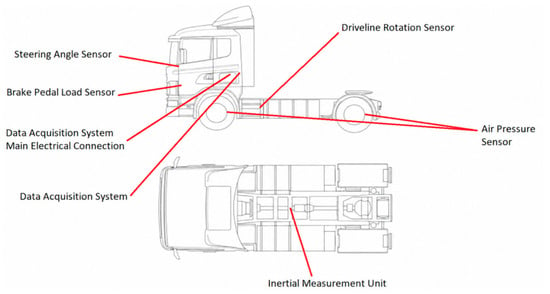
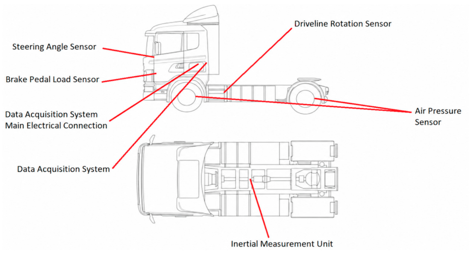
Preliminary on-vehicle system-identification tests were conducted using the instrumented test vehicle to obtain experimental data for calibrating the controller-oriented braking model used in the MIL, SIL, and HIL validation stages. During these tests, the vehicle was equipped with sensors to measure the braking-system inputs and vehicle-response outputs required for system identification. The measured signals included wheel speeds, brake-chamber air pressures, brake-pedal load, longitudinal acceleration, vehicle speed, driveline rotation, steering angle, and inertial measurements. These measurements were used to identify the dominant longitudinal braking dynamics of the vehicle, including pneumatic pressure delay, brake-pressure modulation, wheel deceleration, slip development, and vehicle-speed reduction. A schematic of the sensor locations on the instrumented test vehicle is shown in Figure 2.

Figure 2. Vehicle schematic and sensor placement.

Table 2 below shows the information related to the sensors used on the vehicle for data collection.

Table 2. Sensors used for recording vehicle data.

Sensor	Brand/Model	Manufacturer	Description/Specifications
Inertial Measurement Unit	Duetto Buch GPS100.Mini	DUETTO-Engineering Munich/Germany	GNSS/IMU unit with GPS, 3-axis accelerometer, gyroscope, compass, and pressure sensor; up to 100 Hz output.
Air Pressure Sensor	BCT-22-25B-V-G1/4-S-8M/Atek	ATEK Alfa Kocaeli/Türkiye	0–25 bar pressure sensor; 0–10 V output; 12–30 VDC supply; IP65/IP67.
Inclination Sensor	INC 110 E 02-/+90° PP V CW 3M/Atek	ATEK Alfa Kocaeli/Türkiye	Two-axis ±90° tilt sensor; ±0.2° accuracy; 0–10 V output; IP67.
Steering Angle Sensor	INC 210 A 01 360° PP V CW 3M/Atek	ATEK Alfa Kocaeli/Türkiye	0–360° angle sensor; ±0.1° accuracy; 0–10 V output; IP67.
Pedal Force Sensor	PKF 2.0/HKM Messtechnik	HKM Messtechnik Freiburg/Germany	0–1500 N pedal force sensor; 2 mV/V output; IP65.
Optical RPM Sensor	ROS-W/Monarch Instrument	Monarch Instrument Amherst, NH, USA	Optical speed sensor; 1–250,000 RPM range; 3–15 VDC supply.

The preliminary system-identification tests provided the experimental basis for the subsequent model-development and calibration stages. The measured wheel speeds, brake-chamber pressures, pedal load, acceleration, vehicle speed, and inertial data were used to identify the dominant braking-system behavior and to tune the controller-oriented vehicle, tire, and pneumatic subsystem models. The same data also provided reference values for setting the corresponding vehicle parameters in TruckMaker^®, including the longitudinal resistance terms, brake-pressure response, wheel-speed behavior, and deceleration characteristics. Therefore, the system-identification stage established the link between the real vehicle measurements and the MIL, SIL, and HIL simulation models used in the later validation process.

2.2.1. Pneumatic Subsystem Model

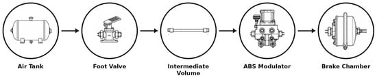
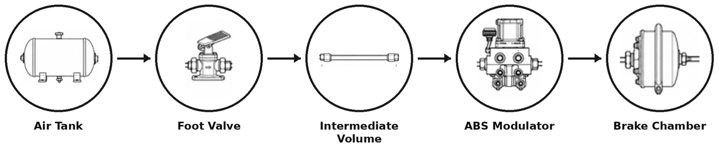
The pneumatic subsystem was first represented by the lumped circuit shown in Figure 3, consisting of the air tank, foot valve, intermediate pneumatic volume, ABS modulator, and brake chamber. In the simplified model used for controller development, the elements after the foot valve and before the ABS modulator were lumped together as a simple volume, whereas the foot valve and the ABS modulator were modeled as simple valves, having an open or closed state (the mechanical subsystem is not modeled). Additionally, the air tank was considered to have constant pressure, and the temperatures at each component were also considered constant.

Figure 3. Lumped pneumatic circuit used for brake-pressure response modeling.

For each pneumatic element, the output pressure was modeled using a valve-state-dependent first-order pressure response:

$${\dot{p}}_{o,i}=\left\{\begin{array}{cc}{\displaystyle \frac{p_{i,i}-p_{o,i}}{{\tau }_{a,i}}},& \mathrm{apply},\\ 0,& \mathrm{hold},\\ -{\displaystyle \frac{p_{o,i}-p_{\mathrm{a}\mathrm{t}\mathrm{m}}}{{\tau }_{e,i}}},& \mathrm{exhaust},\end{array}\right.$$

(2)

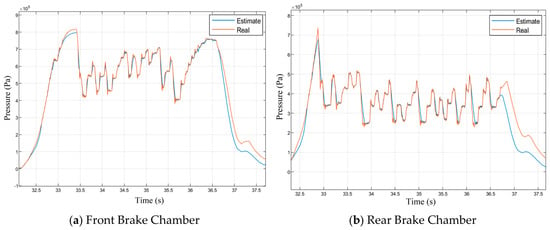
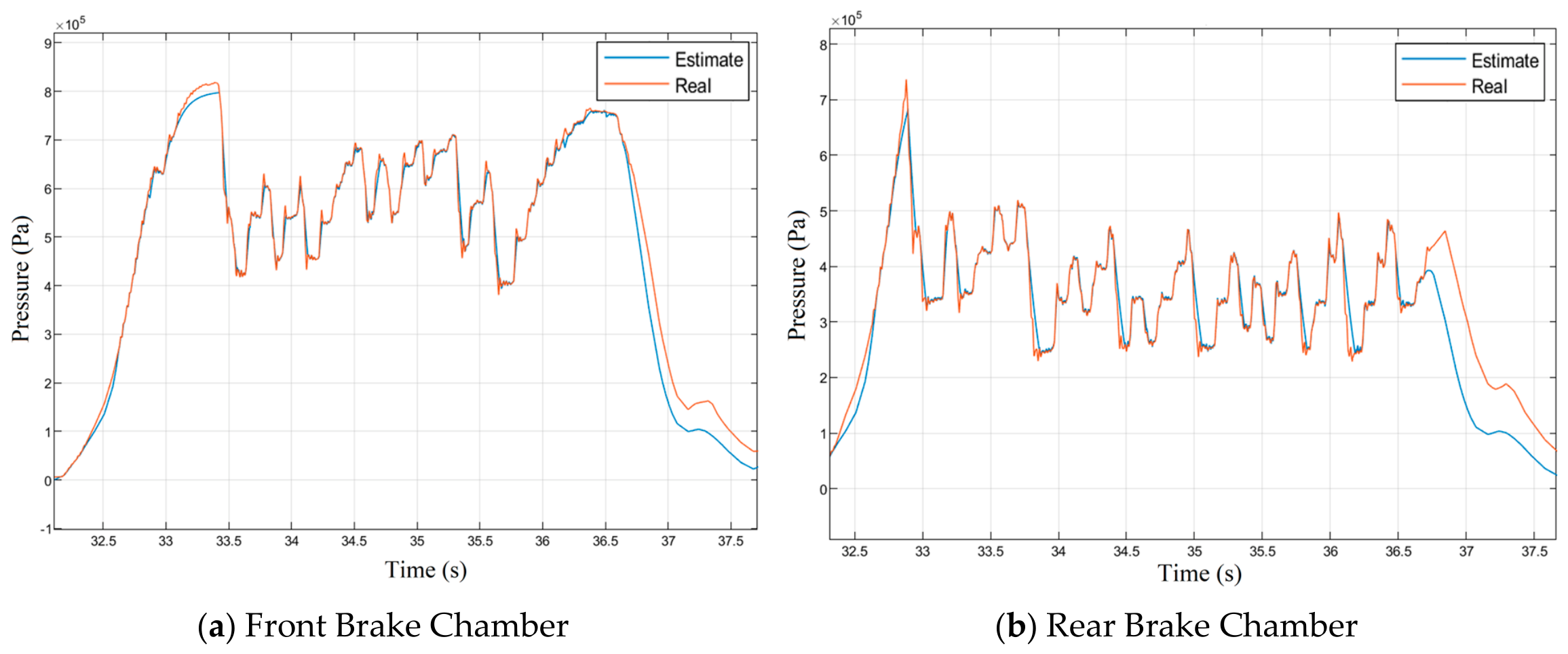
where $p_{i,i}$ is the inlet pressure, $p_{o,i}$ is the outlet pressure, $p_{\mathrm{a}\mathrm{t}\mathrm{m}}$ is atmospheric pressure, and ${\tau }_{a,i}$ and ${\tau }_{e,i}$ are the effective apply and exhaust time constants. This form captures the main behavior required for ABS simulation: pressure does not follow the controller command instantaneously, but reaches the brake chamber through delayed filling, holding, and exhausting dynamics. This simple approach closely approximates the real valve behavior and also removes the need to model the flowrate through the valves, and can be used to simply obtain the pressure gradient at the component at the exit of the valve. The front and rear brake-chamber pressure-response fits shown in Figure 4 were therefore used to tune the effective pneumatic time constants and modulation response. The fits show that the model captures the valve behavior, particularly for the different ABS Apply/Hold/Exhaust cycles. Here, the valve command is obtained using the slope of the real brake pressure.

Figure 4. Comparison of measured and modeled brake-chamber pressure responses for (a) the front chamber and (b) the rear chamber.

The measured pressure responses in Figure 4 were obtained during the instrumented full-vehicle tests described in Section 2.2. Brake-chamber pressures were recorded using the pressure sensors listed in Table 2, installed at the corresponding front and rear brake chambers. The ABS apply, hold, and exhaust commands recorded during the same tests were used as inputs to the first-order pressure model defined in Equation (2). The effective apply and exhaust time constants were adjusted to minimize the difference between the modeled and measured chamber-pressure responses. Therefore, the “actual” curves represent measured vehicle data, while the “predicted” curves represent the model response under the same recorded command sequence and test conditions.

The brake torque at each wheel was related to chamber pressure through an identified brake gain. The brake torque can be expressed as a function of brake-line pressure, pushout pressure, brake chamber diaphragm area, brake factor, mechanical efficiency, leverage ratio, fade factors, and the effective drum radius. These terms can be combined into an equivalent constant. For controller-oriented simulation this can be written as

$$T_{b,i}=k_{b,i}^{\prime }\left(p_{c,i}−p_{0,i}\right),$$

(3)

where $T_{b,i}$ is the braking torque, $p_{c,i}$ is the chamber pressure, $p_{0,i}$ is the pushout or threshold pressure, and $k_{b,i}^{\prime }$ is the identified effective brake gain.

2.2.2. Vehicle Parameters

The longitudinal vehicle model was then calibrated using braking data. The longitudinal equation can be written in terms of front and rear tire forces, rolling resistance, aerodynamic resistance, grade resistance, and a rotary mass factor. In compact form,

$$\gamma m{\dot{v}}_x=-\sum _i{F}_{x,i}-R_r-R_a-R_g,$$

(4)

where $m$ is the vehicle mass, $\gamma$ is the rotary mass factor (additional inertia due to vehicle powertrain), $v_x$ is the longitudinal vehicle speed, $F_{x,i}$ are the longitudinal tire braking forces, $R_r$ is rolling resistance, $R_a$ is aerodynamic resistance, and $R_g$ is grade resistance. The resistance terms may be written as

$$R_a={\displaystyle \frac{1}{2}}\rho C_d{A}_f{v}_x^2,$$

(5)

$$R_r=C_{rr}\mathrm{mgcos}\theta ,$$

(6)

$$R_g=\mathrm{mgsin}\theta ,$$

(7)

where $\rho$ is air density, $C_d$ is drag coefficient, $A_f$ is frontal area, $C_{rr}$ is the rolling-resistance coefficient, and $\theta$ is the road-grade angle. The wheel rotational dynamics were represented as

$$J_i{\dot{\omega }}_i=R_w{F}_{x,i}-T_{b,i},$$

(8)

where $J_i$ is the wheel rotational inertia, ${\omega }_i$ is wheel angular speed, $R_w$ is the wheel radius, $T_{b,i}$ is the brake torque, and $F_{x,i}$ is the longitudinal tire force. The subscript ‘i’ represents the wheels of the vehicle where $i=1, 2, 3, 4$. Table 3 below shows the mapping of the subscript to the vehicle wheels.

Table 3. Wheel Numbers Mapping.

Subscript Number	Wheel
1	Front Left Wheel
2	Front Right Wheel
3	Rear Left Wheel
4	Rear Right Wheel

The longitudinal tire force was represented using the constant-coefficient Pacejka Magic Formula [4]:

$$F_x=F_{z}D\sin \left[C{\mathrm{t}\mathrm{a}\mathrm{n}}^{-1}\left(B\kappa -E\left[B\kappa -{\mathrm{t}\mathrm{a}\mathrm{n}}^{-1}\left(B\kappa \right)\right]\right)\right]$$

(9)

where $F_x$ is the longitudinal tire force, $F_z$ is the vertical tire load, $\kappa$ is the longitudinal slip, and $B$, $C$, $D$, and $E$ are the stiffness, shape, peak, and curvature coefficients, respectively. The coefficient sets used for the evaluated road conditions are listed in Table 4.

Table 4. Magic Formula Parameters.

Surface	B	C	D	E
Dry tarmac	10	1.9	1.00	0.97
Wet tarmac	12	2.3	0.82	1.00
Snow	5	2.0	0.30	1.00
Ice	4	2.0	0.10	1.00

The model parameters were identified using a bounded nonlinear least-squares procedure implemented in MATLAB (version 2024b). The measured brake-chamber pressures, wheel accelerations, and vehicle speed were used as time-varying model inputs, while the vehicle mass, effective wheel radius, frontal area, air density, and road-grade angle were specified from measured or known vehicle data. The recorded brake-chamber pressures were used to calculate the brake torques using Equation (3).

The vehicle-parameter vector was defined as

$${\theta }_v={\left[\begin{array}{cccc}\gamma & C_{rr}& C_d& J_w\end{array}\right]}^T$$

(10)

where $J_w$ represents the common wheel rotational inertia. The effective brake gain was expressed as

$$k_b^{\prime }=s_b{k}_{b,0}^{\prime }$$

(11)

where $k_{b,0}^{\prime }$ is the nominal pressure-to-brake-torque gain calculated from the brake-system geometry and $s_b$ is an estimated dimensionless gain scale.

An alternating two-stage identification procedure was employed to reduce the coupling between the vehicle parameters and the effective brake gain. In the first stage, $s_b$ was fixed at its current value and $\gamma$, $C_{rr}$, $C_d$, and $J_w$ were estimated. In the second stage, the identified vehicle parameters were fixed and $s_b$ was estimated. These two stages were repeated until the maximum relative parameter change was less than 10⁻⁵ and the relative change in the objective function was less than 10⁻⁷. The objective function was defined as the event-normalized squared error between the measured and estimated longitudinal accelerations:

$$J\left({\theta }_v,s_b\right)={\displaystyle \sum _{j=1}^{N_{\mathrm{e}}}}{\displaystyle \frac{1}{N_j}}{\displaystyle \sum _{k=1}^{N_j}}{\left[a_{x,\mathrm{e}\mathrm{s}\mathrm{t}}\left(t_{j,k};{\theta }_v;s_b\right)-a_{x,\mathrm{m}\mathrm{e}\mathrm{a}\mathrm{s}}\left(t_{j,k}\right)\right]}^2$$

(12)

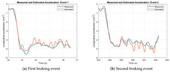
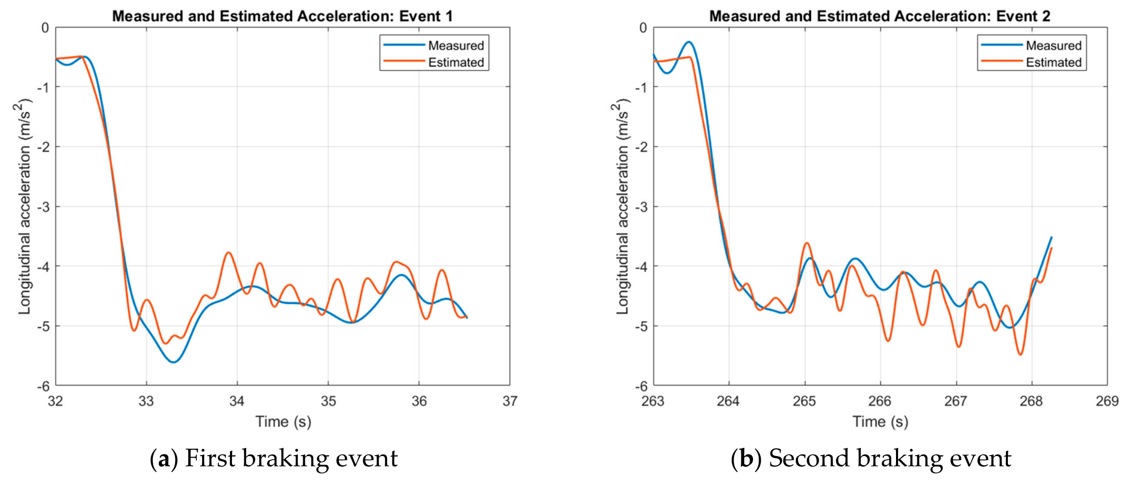
where $N_{\mathrm{e}}$ is the number of braking events and $N_j$ is the number of samples in event $j$. To reduce sensitivity to the initial parameter values, the complete alternating optimization was repeated from 20 initial parameter sets distributed within the specified parameter bounds, and the solution with the lowest objective-function value was retained. The parameters were identified using the two braking events shown in Figure 5.

Figure 5. Comparison of measured and estimated longitudinal acceleration for (a) the first braking event and (b) the second braking event.

The parameter bounds and final identified values are presented in Table 5 and Table 6.

Table 5. Parameter Estimation Output.

Parameter	Initial Value	Lower Bound	Upper Bound	Identified Value
Rotary mass factor, $\gamma$	1.40	1.00	2.00	1.23
Rolling-resistance coefficient, $C_{rr}$	0.005	0.001	0.10	0.042
Aerodynamic drag coefficient, $C_d$	0.70	0.30	1.50	1.17
Common wheel inertia, $J_w$	15.00	5.00	40.00	24.29
Brake-gain scale, $s_b$	1.00	0.50	2.00	0.91

Table 6. Error of Measured vs. Estimated Acceleration.

Braking Instance	Root Mean Square Error
Overall	0.30
First Braking Instance	0.29
Second Braking Instance	0.31

A local one-at-a-time sensitivity analysis was performed to quantify the influence of the identified parameters on the model response. Each parameter, including the brake-gain scale, was independently perturbed by ±5%, while all remaining parameters were maintained at their identified values. For each perturbation, the percentage change in the acceleration RMSE was calculated relative to the nominal calibrated result. The sensitivity results are summarized in Table 7.

Table 7. Parameter Perturbation Results.

Parameter	Perturbation	Nominal Value	Perturbed Value	RMSE
Rotary mass factor, $\gamma$	−5%	1.22	1.17	0.38
Rotary mass factor, $\gamma$	+5%	1.22	1.29	0.35
Rolling-resistance coefficient, $C_{rr}$	−5%	0.04	0.04	0.30
Rolling-resistance coefficient, $C_{rr}$	+5%	0.04	0.04	0.30
Aerodynamic drag coefficient, $C_d$	−5%	1.17	1.11	0.30
Aerodynamic drag coefficient, $C_d$	+5%	1.17	1.23	0.30
Common wheel inertia, $J_w$	−5%	24.29	23.08	0.30
Common wheel inertia, $J_w$	+5%	24.29	25.51	0.30
Brake-gain scale, $s_b$	−5%	0.90	0.86	0.35
Brake-gain scale, $s_b$	+5%	0.90	0.95	0.36

The sensitivity analysis shows that the calibrated response was most strongly influenced by the rotary mass factor and the brake-gain scale. Perturbations in the rotary mass factor produced RMSE values between 0.35 and 0.38, corresponding to absolute increases of approximately 0.053–0.079 above the nominal RMSE level of about 0.300. Similarly, perturbations in the brake-gain scale resulted in RMSE values between 0.35 and 0.36, representing absolute increases of approximately 0.051–0.064. In contrast, perturbations in $C_{rr}$, $C_d$, and $J_w$ yielded RMSE values between 0.30 and 0.30, with absolute deviations from 0.300 of less than 0.001. These results indicate comparatively low local sensitivity to these parameters over the evaluated braking intervals.

2.2.3. Vehicle Speed Estimation

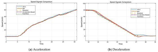
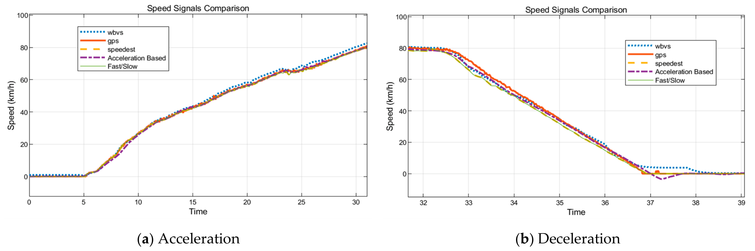
Vehicle-speed estimation was treated as a separate calibration task because the longitudinal slip calculation depends directly on the reference vehicle speed, $v_x$. Figure 6 compares several candidate speed signals. The signal denoted as ‘wbvs’ is the vehicle-speed estimate reported by the commercial WABCO^® ECU (Manufactured by ZF WABCO^® in Bern, Switzerland). The ‘gps’ signal is the speed measured by the external positioning/inertial sensor package. The ‘speedest’ signal is a complex speed-estimation method, which uses wheel-speed peak detection to estimate the vehicle deceleration to obtain a more robust reference speed during braking. The ‘acceleration-based’ signal is obtained by direct integration of the measured longitudinal acceleration, while the ‘fast/slow’ logic selects the fastest or slowest wheel-speed signal depending on the driving condition, for example using the fastest wheel during braking and the slowest wheel during acceleration. The formula for speed estimation is given as below.

$$v_{est}=\left\{\begin{array}{c}\begin{array}{cc}{R}_{w}min\left(\right[{\omega }_{FL},{\omega }_{FR},{\omega }_{RL},{\omega }_{RR}\left]\right)& if \dot{v}>0\end{array}\\ R_w\begin{array}{cc}max\left(\right[{\omega }_{FL},{\omega }_{FR},{\omega }_{RL},{\omega }_{RR}\left]\right)& if \dot{v}<0\end{array}\end{array}\right.$$

(13)

where, $v_{est}$ is the estimated speed, $[{\omega }_{FL},{\omega }_{FR},{\omega }_{RL},{\omega }_{RR}]$ are the front-left, front-right, rear-left, and rear-right wheel speeds respectively, $R_w$ is the wheel radius, and $\dot{v}$ is the vehicle acceleration.

Figure 6. Vehicle-speed estimation algorithms comparison using the real vehicle for (a) Acceleration, and (b) Deceleration.

Wheel-speed-based vehicle-reference-speed estimation is also consistent with practical ABS implementation, where the vehicle speed is not normally measured directly by a dedicated vehicle-speed sensor during braking. Patent literature related to commercial ABS systems describes similar principles. In a WABCO^® patent, the vehicle reference speed is described as being generally based on the highest wheel speed during normal or lightly braked operation, while a slope-limited reference curve is used when wheel deceleration is faster than physically possible for the vehicle body [34]. Similarly, another ABS reference-speed method checks the integrity of individual wheel-speed signals and bounds the decrease in the reference speed so that the estimate cannot decelerate faster than a physically possible vehicle-body deceleration [35]. Therefore, the fastest/slowest-wheel algorithm is chosen as a practical low-complexity speed estimation approach. In implementation, the selected wheel-speed-based estimate was combined with rate-limiting logic to prevent sudden non-physical drops in the estimated vehicle speed if one or more wheels approach lock-up.

$${\hat{v}}_k=\max \left(v_{\mathrm{s}\mathrm{e}\mathrm{l},k},{\hat{v}}_{k-1}-a_{\mathrm{l}\mathrm{i}\mathrm{m}}\Delta t\right)$$

(14)

where ${\hat{v}}_k$ is the rate-limited vehicle-speed estimate at sample $k$, $v_{\mathrm{s}\mathrm{e}\mathrm{l},k}$ is the selected wheel-speed-based estimate, $a_{\mathrm{l}\mathrm{i}\mathrm{m}}$ is the maximum allowable reference-speed deceleration, and $\Delta t$ is the sampling time.

The comparison in Figure 6 shows that the selected low-complexity estimator follows the main vehicle-speed trend with acceptable agreement for the intended controller-development workflow. GPS and acceleration-based estimates are useful references, but GPS may include delay and bandwidth limitations, while acceleration integration is sensitive to bias and drift. The more complex speed-estimation candidate can improve robustness, but it also increases implementation and calibration effort. Therefore, the selected estimator was adopted as a practical embedded solution with limited sensor requirements. In addition, the estimator was exercised in the MIL and HIL braking scenarios, including high-mu, low-mu, split-mu, jump-mu, and cornering cases, where it provided a bounded and physically reasonable reference-speed signal for slip calculation and ABS pressure modulation.

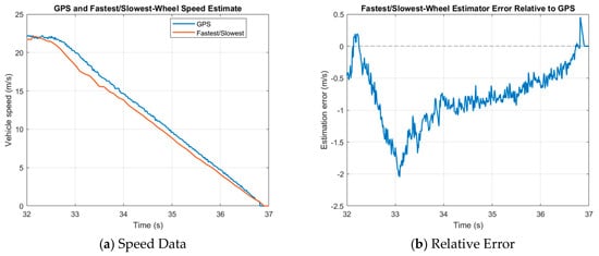
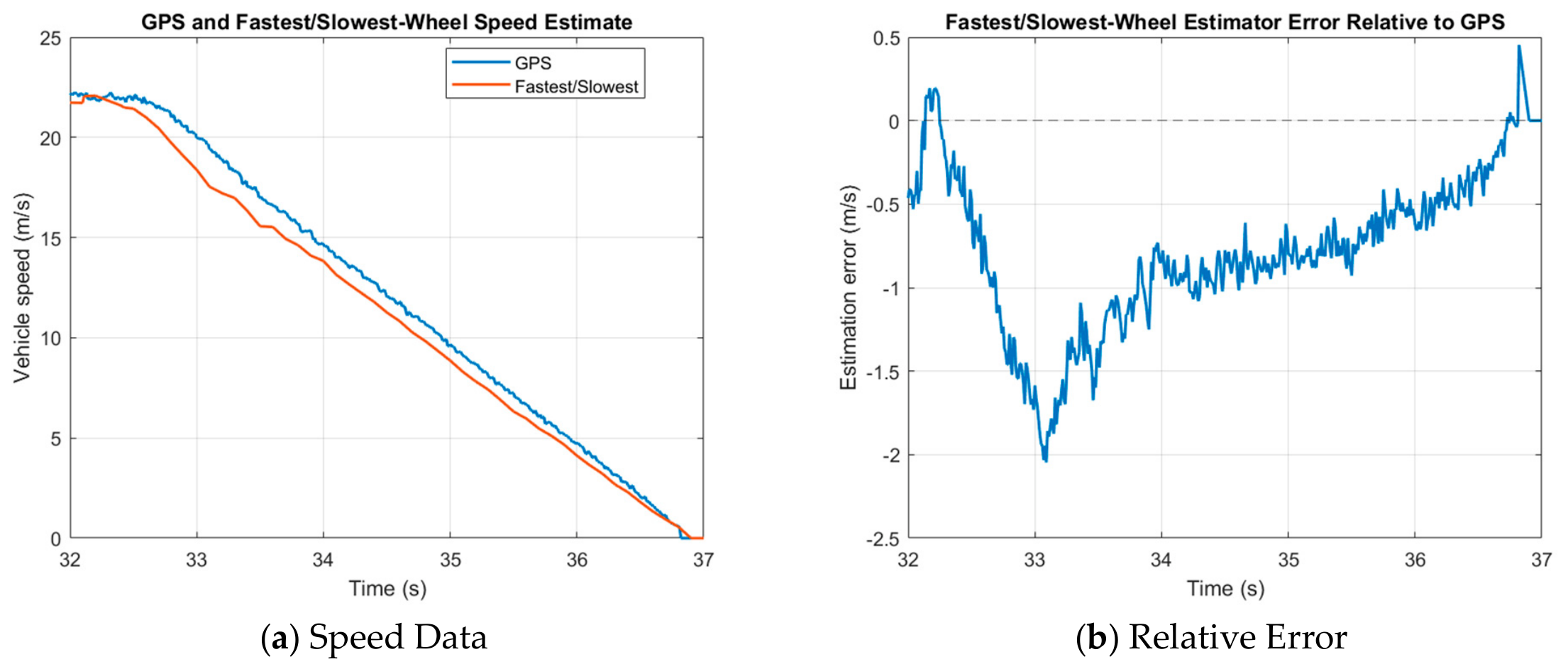
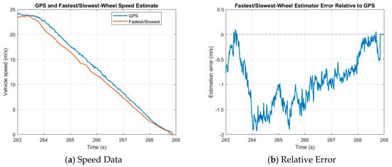
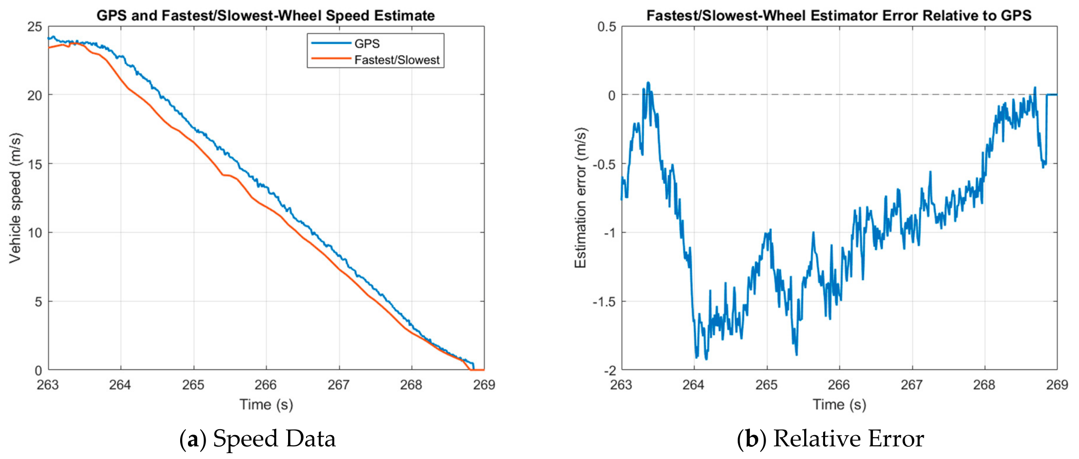
Figure 7 and Figure 8 below show (a) the vehicle speed estimation comparing the GPS speed (blue) and the fastest/slowest speed estimation algorithm (red) for the first and second brake events, and (b) the errors relative to the GPS speed.

Figure 7. Speed Estimation Comparison, (a) First Braking event, (b) Error relative to GPS speed.

Figure 8. Speed Estimation Comparison, (a) Second Braking event, (b) Error relative to GPS speed.

Across the two zoomed braking intervals, the fastest/slowest-wheel estimator closely approximated the real vehicle speed measured using the GPS. During the first braking event (32–37 s), the estimation error ranged from approximately −2.1 to +0.4 m/s, with the maximum absolute deviation occurring near 33 s. During the second braking event (263–269 s), the error ranged from approximately −1.9 to +0.1 m/s, with the largest deviation occurring near 264 s. In both events, the error generally decreased during the later stages of braking, indicating that the estimator captured the overall speed-reduction behavior while temporarily underestimating the vehicle speed during the early and intermediate braking phases. Overall, the speed estimate is able to provide a reasonable reference speed, which can be used for estimating the wheel slips.

2.2.4. Tire Force–Slip Model

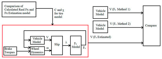
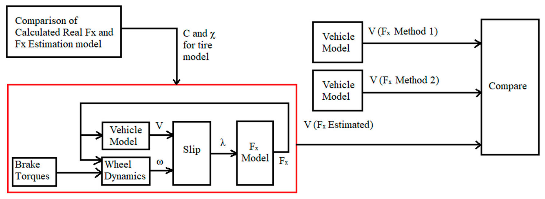
The longitudinal tire force–slip relationship was identified from experimental braking data to obtain a calibrated tire model for ABS simulation and validation. The model describes the longitudinal tire force, $F_x$, as a function of the longitudinal slip ratio, $\kappa$. The calibration procedure used two complementary force-estimation methods and compared their results with a reduced-order tire model as shown in Figure 9.

Figure 9. Tire-model calibration and validation procedure used to identify the longitudinal force–slip relationship. The red-outlined block shows the procedure used to generate the tire-model estimate of the longitudinal force, $F_x$, from the brake torque, vehicle longitudinal velocity $V$, wheel angular velocity $\omega$, and calculated longitudinal slip ratio $\lambda$. The estimated is then compared with two independent methods used to estimate the actual longitudinal tire force. Arrows indicate the direction of signal/data flow. and denote the calibrated tire-model parameters.

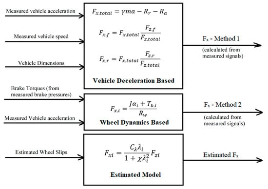
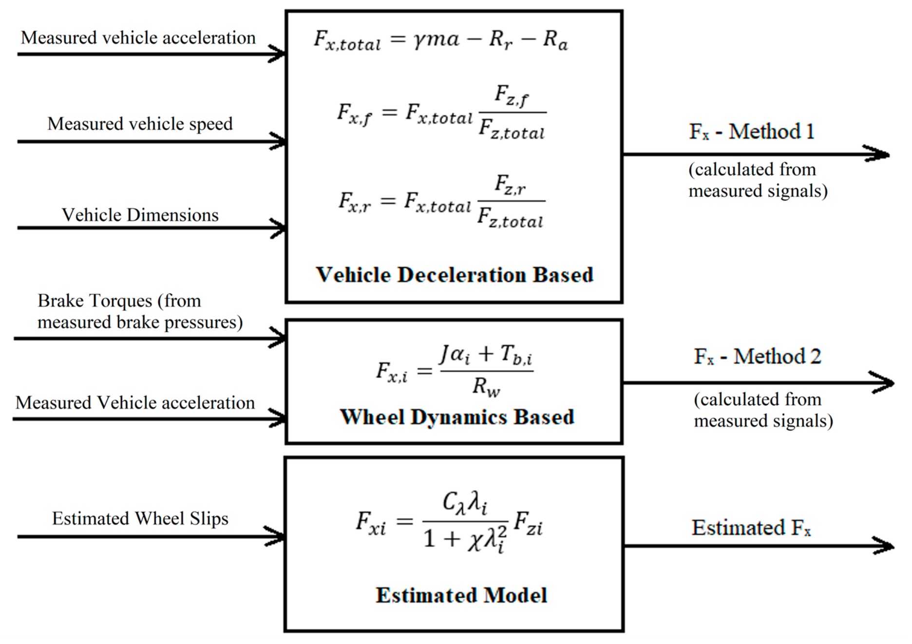
The first force estimate was obtained from the measured vehicle deceleration. With the adopted braking-force sign convention, the total longitudinal braking force is expressed as

$$F_{x,\mathrm{t}\mathrm{o}\mathrm{t}\mathrm{a}\mathrm{l}}=-\gamma m{\dot{v}}_x-R_r-R_a-R_g,$$

(15)

The total force was distributed between the front and rear axles according to the dynamic normal loads:

$$F_{x,f}=F_{x,\mathrm{t}\mathrm{o}\mathrm{t}\mathrm{a}\mathrm{l}}{\displaystyle \frac{F_{z,f}}{F_{z,\mathrm{t}\mathrm{o}\mathrm{t}\mathrm{a}\mathrm{l}}}}, F_{x,r}=F_{x,\mathrm{t}\mathrm{o}\mathrm{t}\mathrm{a}\mathrm{l}}{\displaystyle \frac{F_{z,r}}{F_{z,\mathrm{t}\mathrm{o}\mathrm{t}\mathrm{a}\mathrm{l}}}}$$

(16)

For straight-line braking, the dynamic axle loads were approximated as

$$F_{z,f}={\displaystyle \frac{b}{L}}mg+{\displaystyle \frac{h}{L}}m{a}_b,$$

(17)

$$F_{z,r}={\displaystyle \frac{a}{L}}mg-{\displaystyle \frac{h}{L}}m{a}_b,$$

(18)

where $L=a+b$ is the wheelbase, $a$ and $b$ are the distances from the front and rear axles to the center of gravity, $h$ is the center-of-gravity height, and $a_b=-{\dot{v}}_x$ is the braking deceleration. This approach is referred to as Method 1. The second method estimated the wheel-level longitudinal force from wheel rotational dynamics:

$$F_{x,i}={\displaystyle \frac{T_{b,i}+J_i{\dot{\omega }}_i}{R_w}},$$

(19)

where $T_{b,i}$ is the brake torque, $J_i$ is the wheel inertia, ${\omega }_i$ is the wheel angular speed, and $R_w$ is the effective wheel radius. This approach is referred to as Method 2. Both methods are shown in Figure 10.

Figure 10. Longitudinal tire-force estimation structure. Method 1 estimates the longitudinal tire force from the measured vehicle deceleration, whereas Method 2 estimates the longitudinal tire force from the wheel dynamics and measured brake torque. The estimated model calculates the longitudinal tire force from the estimated wheel slip using the calibrated tire-model parameters.

The calibrated tire model was represented using the following compact rational form:

$$F_{x,i}=F_{z,i}{\displaystyle \frac{C_i{\lambda }_i}{1+{\chi }_i{\lambda }_i^2}},$$

(20)

where $F_{x,i}$ is the longitudinal tire force, $F_{z,i}$ is the normal load on the wheel, and ${\lambda }_i$ is the longitudinal slip ratio. The coefficient $C_i$ defines the normalized initial longitudinal stiffness. For small slip values, the denominator is close to one, so the model behaves approximately as $F_{x,i}\approx F_{z,i}{C}_i{\lambda }_i$. Therefore, $C_i$ mainly controls the slope of the force–slip curve in the linear low-slip region. The coefficient ${\chi }_i$ controls the nonlinear saturation behavior by limiting the force growth as slip increases. A larger ${\chi }_i$ causes the tire force to reach its peak at a lower slip value, while a smaller ${\chi }_i$ produces a slower transition toward saturation.

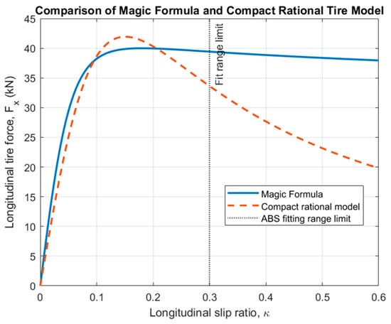
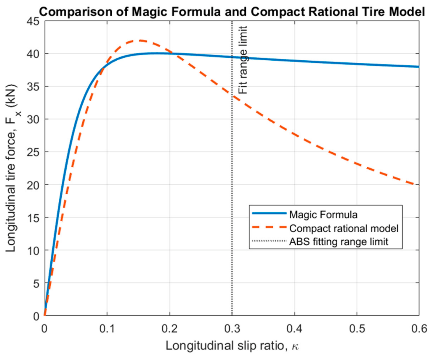
This reduced-order model was selected because it captures the main tire behavior required for ABS-oriented simulations: linear force build-up at low slip, a peak-force region, and reduced force growth at higher slip. Compared with the standard Magic Formula, the compact rational model uses fewer parameters and is easier to calibrate from braking-test data. It is therefore suitable for controller-development simulations where the objective is not to reproduce the full tire characteristic in every operating condition, but to represent the force–slip behavior in the slip range where ABS pressure modulation occurs.

Figure 11 shows the comparison between the standard Magic Formula longitudinal tire model and the compact rational tire model used for ABS-oriented simulation. The rational model is fitted over the braking slip range and captures the main low-slip stiffness and peak-slip behavior with only two calibration parameters, $C_i$ and ${\chi }_i$.

Figure 11. Comparison of the rational tire formula and magic formula.

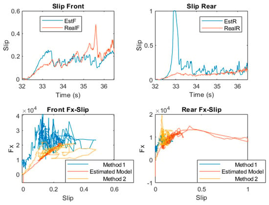
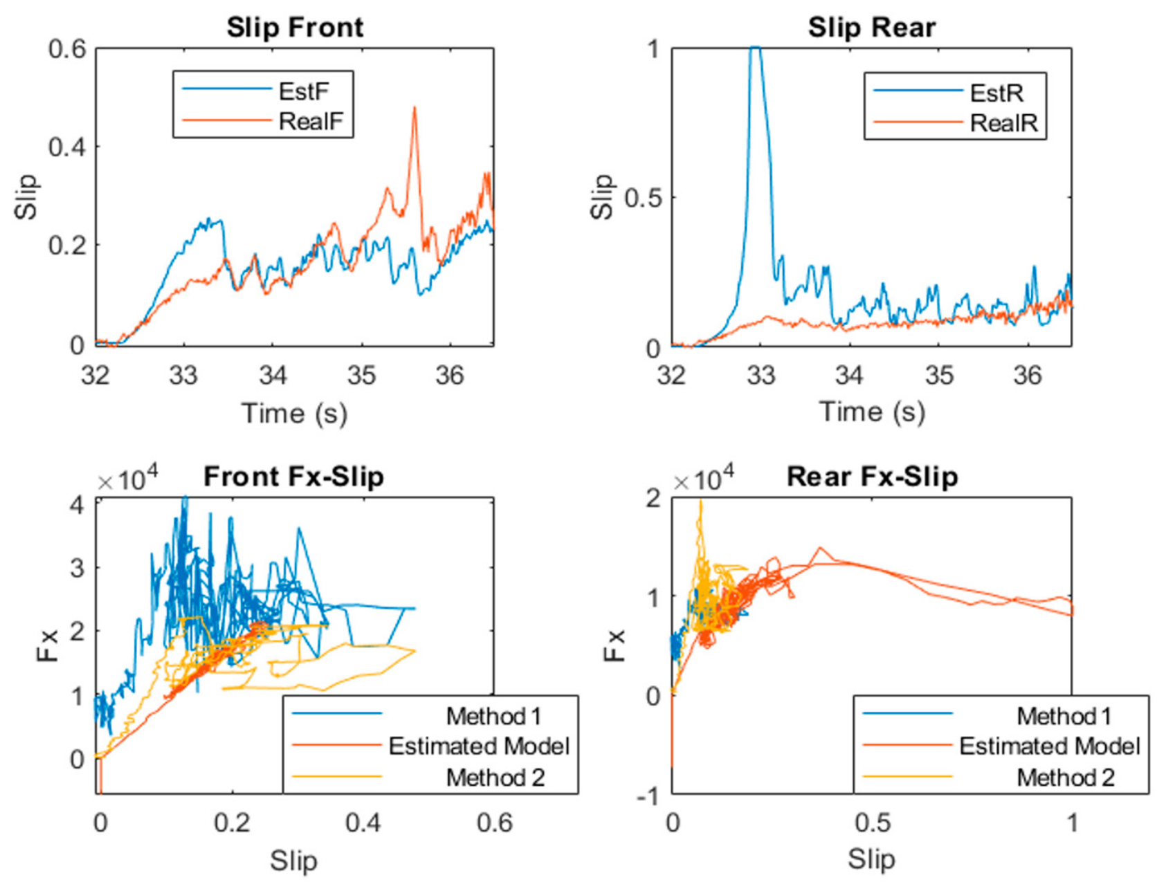
The estimated force–slip curves are compared in Figure 12. The calibrated model follows the main trend of both experimental estimates, especially in the low-slip region where the force build-up is approximately linear. The vehicle-deceleration-based estimate shows larger scatter because it depends on differentiated vehicle-speed data and dynamic load-transfer assumptions.

Figure 12. Comparison of the measured and estimated tire forces.

The wheel-dynamics-based estimate provides a more direct wheel-level comparison but remains sensitive to wheel-speed resolution and angular-acceleration noise. Here, ‘EstF’ and ‘EstR’ are the estimated slips obtained using the estimated tire force, ‘RealF’ and ‘RealR’ are the wheel slips obtained from the measured data, while the lower two plots show the tire longitudinal forces against the slips.

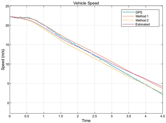
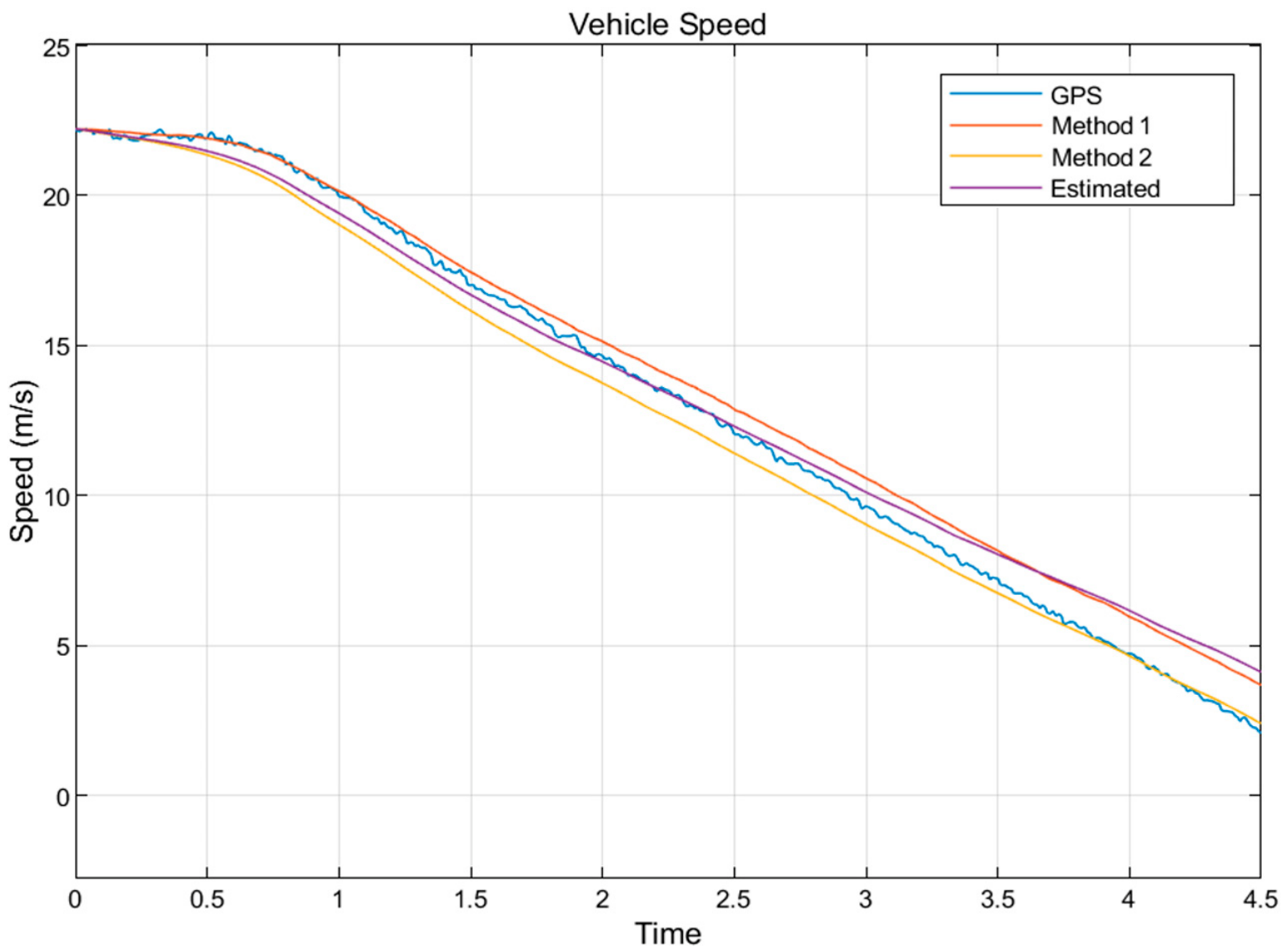
Finally, the calibrated braking model was validated by comparing the simulated vehicle-speed response with the measured GPS speed shown in Figure 13. This validation is necessary because matching the force–slip curve alone does not ensure that the complete braking plant reproduces the measured deceleration and slip evolution. The vehicle-speed comparison shows acceptable agreement between the calibrated model and the measured GPS response. Method 2 gives a particularly close speed trend, while Method 1 provides an independent vehicle-level consistency check. The remaining deviations are mainly attributed to sensor noise, limited wheel-speed resolution, numerical differentiation, and simplified load-transfer and resistance assumptions. The calibrated plant model was then retained through the MIL, SIL, and HIL validation stages to ensure that controller performance was evaluated against a consistent braking-plant representation.

Figure 13. Vehicle-speed comparison after calibration of the braking model.

Table 8 below gives the identified parameters for the tire force–slip model.

Table 8. Tire force–slip estimated parameters.

Parameter	Front Wheels	Rear Wheels
$C_i$	3	6
${\chi }_i$	3	10

2.3. Vehicle, Tire and Pneumatic Simulation Models

The simulation plant combined a 4 × 4 vehicle-dynamics model, tire-force model, pneumatic brake model, and ABS controller implementation. In the MIL environment, the vehicle was represented using a Newton–Euler formulation in MATLAB/Simulink, including the wheel model, Newton–Euler vehicle equations, suspension-force calculation, axle-force calculation, and pneumatic/brake-torque blocks.

The MIL vehicle model used translational and rotational Newton–Euler equations of motion. In compact form, the vehicle translational dynamics can be written as

$$m\left(\dot{\mathbf{v}}+\mathit{\omega }\times \mathbf{v}\right)=\sum \mathbf{F},$$

(21)

where $m$ is the vehicle mass, $\mathbf{v}=[u\mid v\mid w{]}^T$ is the velocity vector in the body-fixed frame, $\mathit{\omega }=[p\mid q\mid r{]}^T$ is the roll, pitch, and yaw-rate vector, and $\sum \mathbf{F}$ is the resultant force vector from tires, suspension, gravity, aerodynamic resistance, and braking. The rotational dynamics can be written as

$$\mathbf{I}\dot{\mathit{\omega }}+\mathit{\omega }\times \left(\mathbf{I}\mathit{\omega }\right)=\sum \mathbf{M},$$

(22)

where $\mathbf{I}$ is the vehicle inertia matrix and $\sum \mathbf{M}$ is the resultant moment vector about the vehicle center of gravity. The complete Newton–Euler model was used in MIL to evaluate not only straight-line braking, but also yaw response, lateral motion, and braking under asymmetric friction conditions. Tire forces were represented using the Magic Formula for longitudinal tire force, tire cornering stiffness for lateral force, and some shaping factors used to implement the combined slip approach, given as below for the $i^{th}$ wheel.

$$F_{x,i}=F_{x,i,o}{\displaystyle \frac{1}{{\alpha }^2\chi +1}}, F_{y,i}=F_{y,o}{\displaystyle \frac{1}{{\lambda }^2\eta +1}}$$

(23)

The Magic Formula for longitudinal force can be written as

$$F_{x,i,o}\left(\kappa \right)=F_{z,i}\mathrm{Dsin}\left[C{\mathrm{t}\mathrm{a}\mathrm{n}}^{-1}\left(B\kappa −E\left(B\kappa -{\mathrm{t}\mathrm{a}\mathrm{n}}^{-1}\left(B\kappa \right)\right)\right)\right],$$

(24)

where $B$, $C$, $D$, and $E$ are the stiffness, shape, peak, and curvature parameters. The lateral force is given as below.

$$F_{y,i}=C_{\alpha }\alpha$$

(25)

where, $C_{\alpha }$ is the cornering stiffness, and $\alpha$ is the tire side slip angle.

The pneumatic brake model was developed using the simplified model given in Equation (2). The reduced model preserves the dominant pneumatic behavior relevant to ABS development—pressure build-up delay, pressure hold, and pressure release—without requiring a full real-time solution of compressible flow through every line and valve.

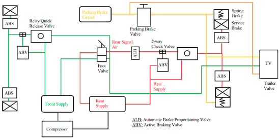
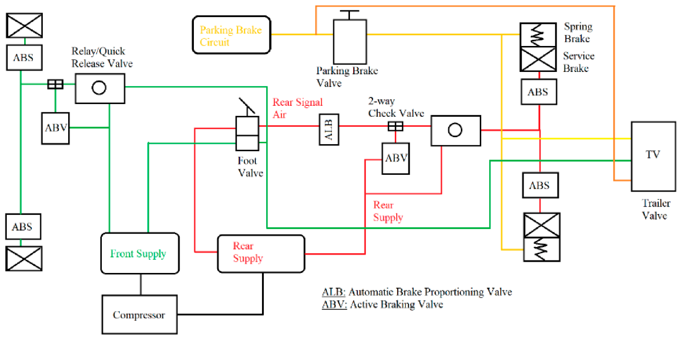
The final pneumatic brake-circuit representation used in the simulation and HIL stages is shown in Figure 14. The green lines represent the front service-brake supply/control path, the red lines represent the rear service-brake supply and signal-air path, and the yellow/orange lines represent the parking-brake, spring-brake, and trailer-related circuit paths. The black symbols denote valves, reservoirs, chambers, and connection elements.

Figure 14. Pneumatic Circuit Layout diagram. The green lines show the front or secondary brake circuit, the red lines show the rear or the primary brake circuit, while the yellow lines indicate the parking brakes circuit. All lines indicate pneumatic connections. The orange lines indicate the connection to the trailer valve/trailer. Boxes with a cross represent service brakes or brake chambers. Boxes with a spring like symbol represent spring/parking brakes. Boxes with a circle in the middle indicate a relay or quick release valve.

The simulation plant also included road-friction profiles for high-$\mu$, low-$\mu$, split-$\mu$, jump-$\mu$, and checkerboard conditions. In split-$\mu$ braking, select-low braking logic was used to reduce the yaw moment generated by unequal left/right braking capacity.

The aim was not only to minimize stopping distance, but also to evaluate whether the controller preserved steerability and yaw stability when the available road friction differed between the left and right sides of the vehicle.

2.4. HIL Simulation Environment

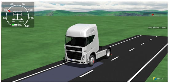
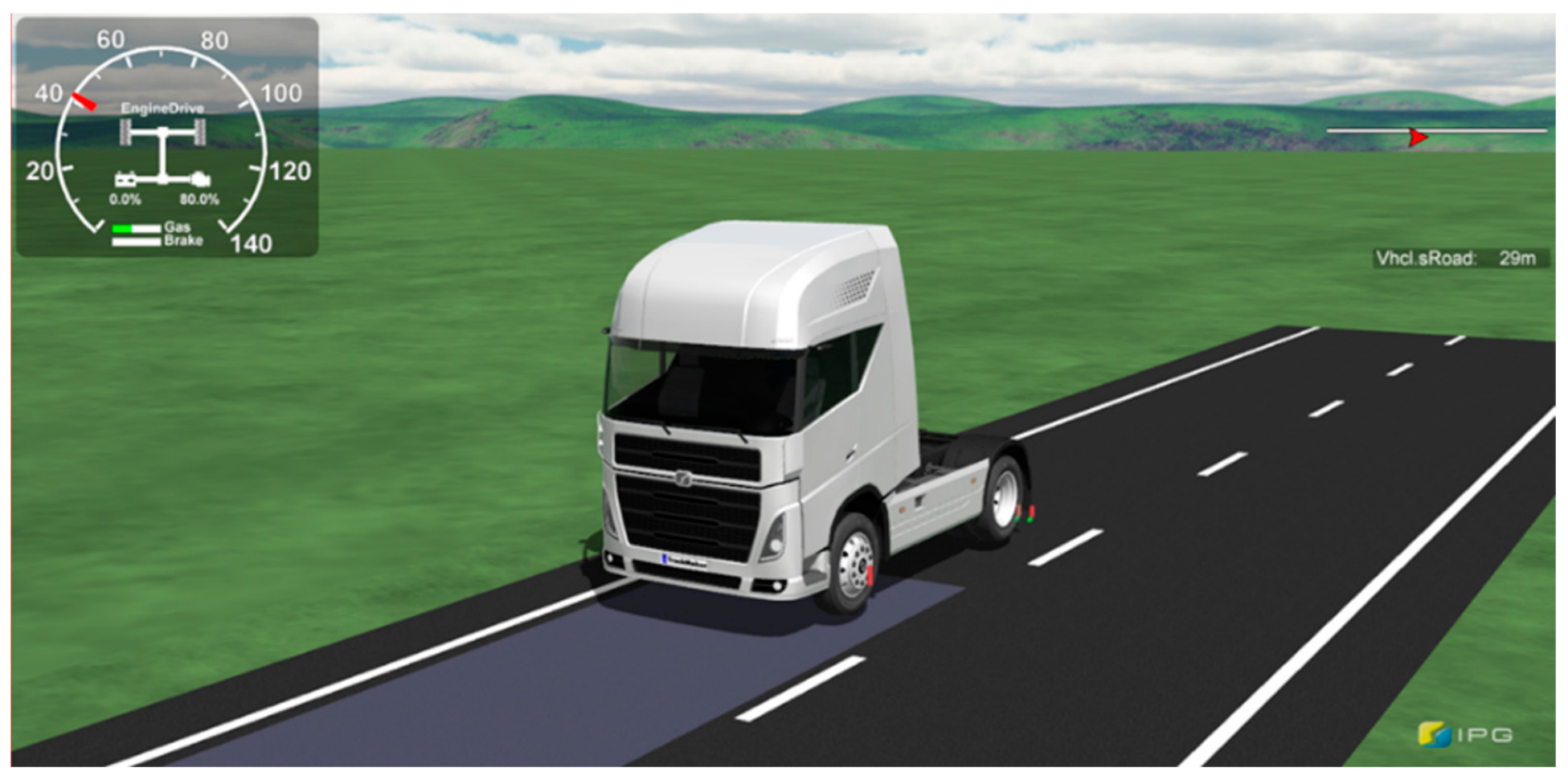
In the HIL environment, the vehicle plant was implemented using TruckMaker^®, as shown in Figure 15. Although the implementation environment is different from the MIL validation, both approaches calculate the vehicle response from tire forces, road inputs, suspension loads, braking torques, and driver or controller commands.

Figure 15. Hardware-in-The-Loop (HIL) Vehicle Model in TruckMaker^®.

The pneumatic circuit has the same layout as the one shown in Figure 14.

For the HIL simulation, the physical ECU exchanged the following signal groups with the HIL simulator and pneumatic bench given below in Table 9.

Table 9. ECU Input and Output signals.

Signal Group	ECU Direction	Role in HIL Validation
Wheel-speed signals	Input	Emulate the four wheel-speed sensor channels used by the ABS algorithm
Brake-demand/pedal signal	Input	Represents driver braking request and enables braking-event detection
ABS modulator inlet-valve commands	Output	Command pressure build-up or apply behavior in each regulated brake channel
ABS modulator outlet-valve commands	Output	Command pressure release or exhaust behavior in each regulated brake channel
Auxiliary valve commands	Output	Drive additional pneumatic elements, such as active braking or relay/quick-release functions, where applicable
CAN/J1939 and diagnostic lines	Bidirectional	Exchange status, diagnostic, and monitoring information
Power, ignition, and ground lines	Input	Provide ECU operating power and enable realistic bench-level startup behavior

The pneumatic bench used in the HIL setup reproduced the main service-brake pneumatic path of the vehicle while excluding trailer-related components. The circuit consisted of the air compressor, air dryer, air reservoirs, four-circuit protection valve, brake pedal and foot brake valve, relay valves, quick-release valve, ABS solenoid modulator valves, auxiliary/ATC solenoid valve, check valves, pneumatic lines, and the brake chambers. In this arrangement, the compressor and reservoirs supplied compressed air, the protection valve distributed the supply to the brake circuits, the foot brake valve generated the driver brake-demand pressure, and the relay and quick-release valves shaped the pressure build-up and exhaust dynamics. The ABS solenoid valves were driven by the physical ECU and modulated the chamber pressure by commanding pressure apply, hold, and release states.

The brake chambers were selected and adjusted to represent those installed on the vehicle. Because each chamber is mechanically coupled to the drum-brake mechanism, it cannot be represented solely as a free pneumatic volume; the compliance and reaction force of the brake mechanism must also be reproduced. The measured brake-chamber pressure–stroke relationship was therefore obtained from static tests, in which the pushout point, brake-engagement point, and maximum-stroke point were identified. The brake chamber converts pneumatic pressure into pushrod force through the effective diaphragm area:

$$F_p=P{A}_{\mathrm{d}\mathrm{i}\mathrm{a}\mathrm{p}\mathrm{h}}$$

(26)

where $F_p$ is the chamber pushrod force, $P$ is the chamber pressure, and $A_{\mathrm{d}\mathrm{i}\mathrm{a}\mathrm{p}\mathrm{h}}$ is the effective diaphragm area. Since the real drum-brake mechanism resists the chamber piston motion, the actuator was also represented with an equivalent stiffness obtained from pressure–stroke data:

$$k={\displaystyle \frac{\Delta F_p}{\Delta x}}$$

(27)

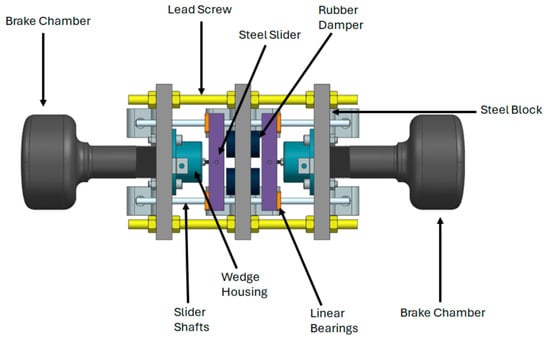
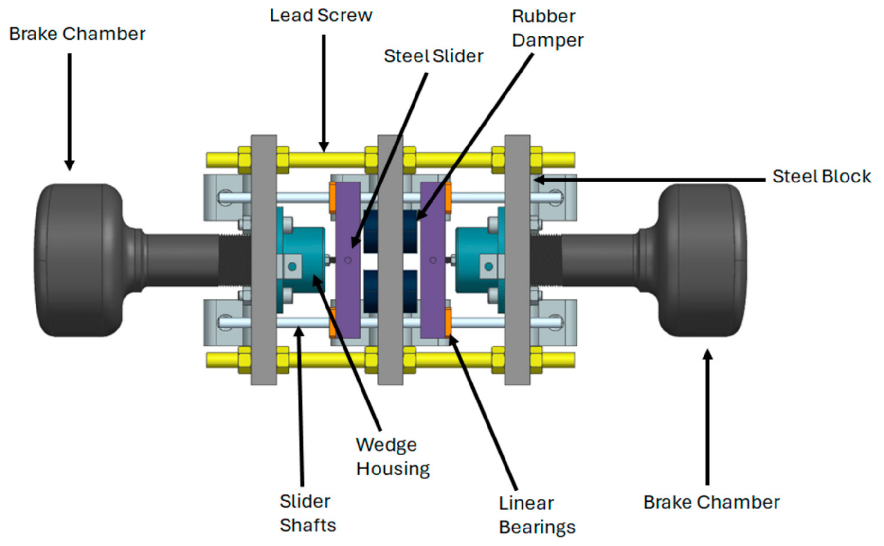
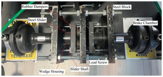
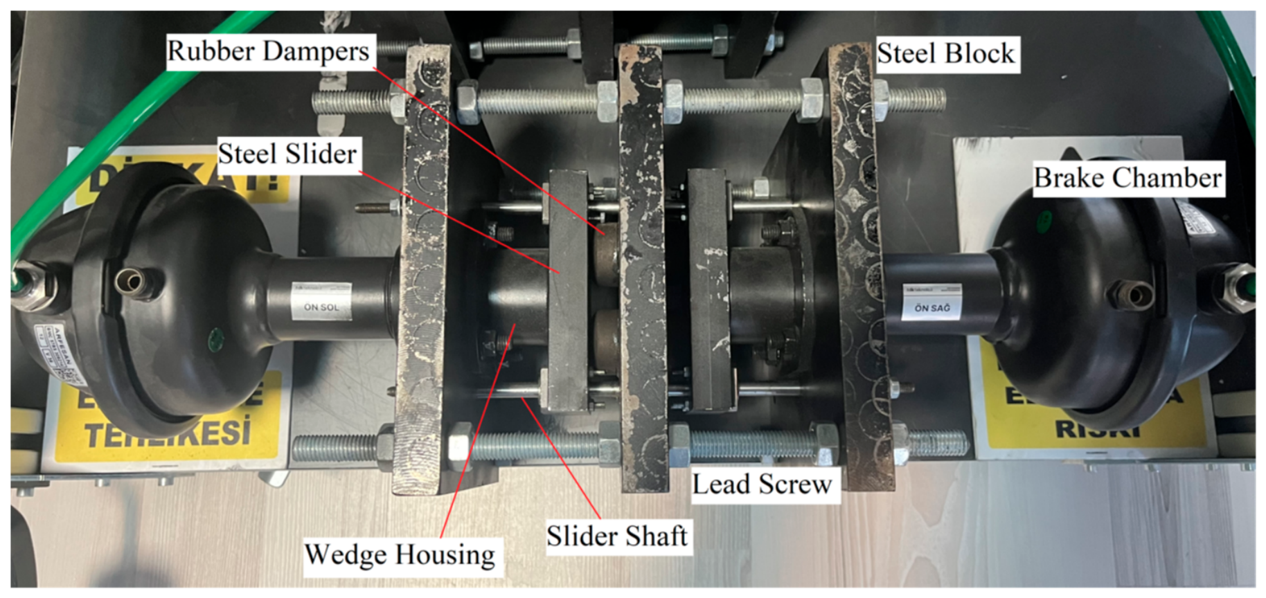
This stiffness was used to reproduce the real brake chamber push-out, engagement, and maximum-stroke behavior in the HIL pneumatic bench. Thus, the chamber model represented both pneumatic pressure generation and the mechanical compliance of the real drum-brake actuator. The HIL brake-chamber assembly was then fitted with equivalent elastic/viscoelastic elements so that the measured piston displacement and pressure rise followed the real chamber response. This adjustment allowed the pneumatic bench to reproduce not only the ECU-controlled pressure modulation, but also the actuator-side resistance and delay introduced by the real drum-brake hardware. The brake chamber schematic is shown below in Figure 16, and the real assembly is shown in Figure 17.

Figure 16. Brake chamber assembly schematic used in the HIL pneumatic bench.

Figure 17. Real brake chamber assembly used in the HIL pneumatic bench.

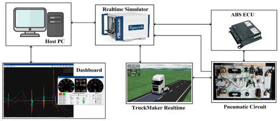
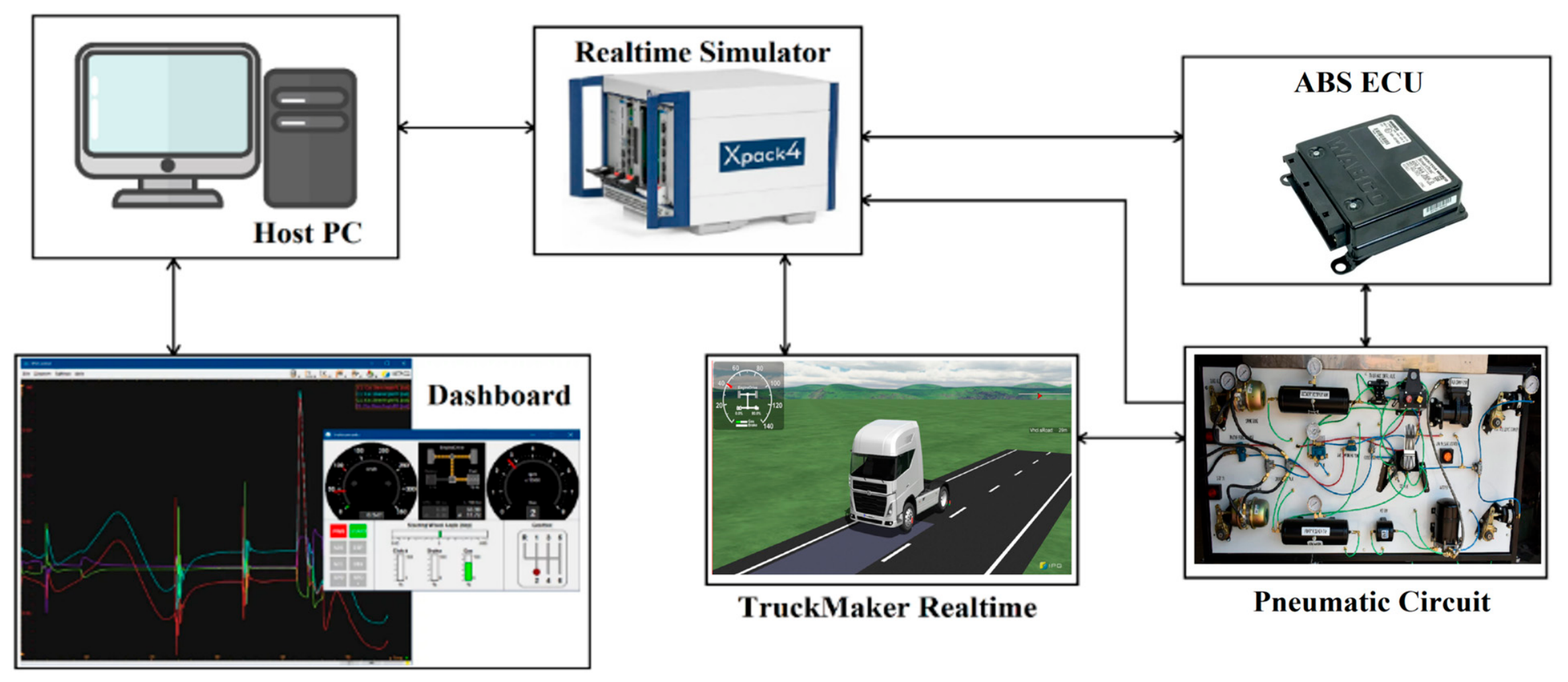
The HIL bench architecture is shown in Figure 18. The host PC was used for configuration, monitoring, and dashboard visualization; the real-time simulator executed the TruckMaker^® vehicle model; the ABS ECU ran the embedded controller code; and the pneumatic circuit provided the actuator-side pressure response. This setup allowed the controller to be tested with realistic wheel-speed inputs, brake-demand signals, modulator commands, pneumatic delays, and diagnostic interfaces before field testing.

Figure 18. Hardware-in-the-loop bench architecture, comprising the host PC, real-time simulator, ABS ECU, pneumatic braking circuit, TruckMaker Realtime vehicle-model interface, and monitoring dashboard. The arrows indicate the communication and signal exchange between the individual hardware and software components. The photographs and software-interface screenshots are representative illustrations of the corresponding components.

2.5. ABS Control Strategies

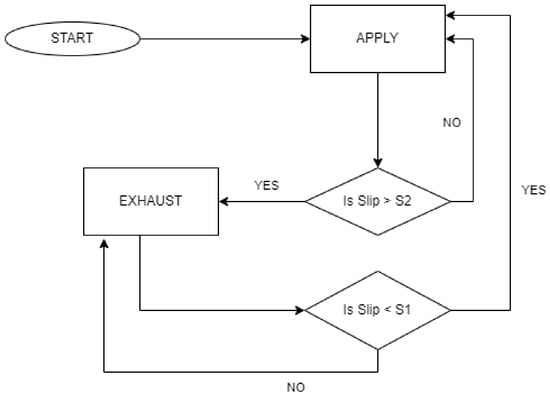
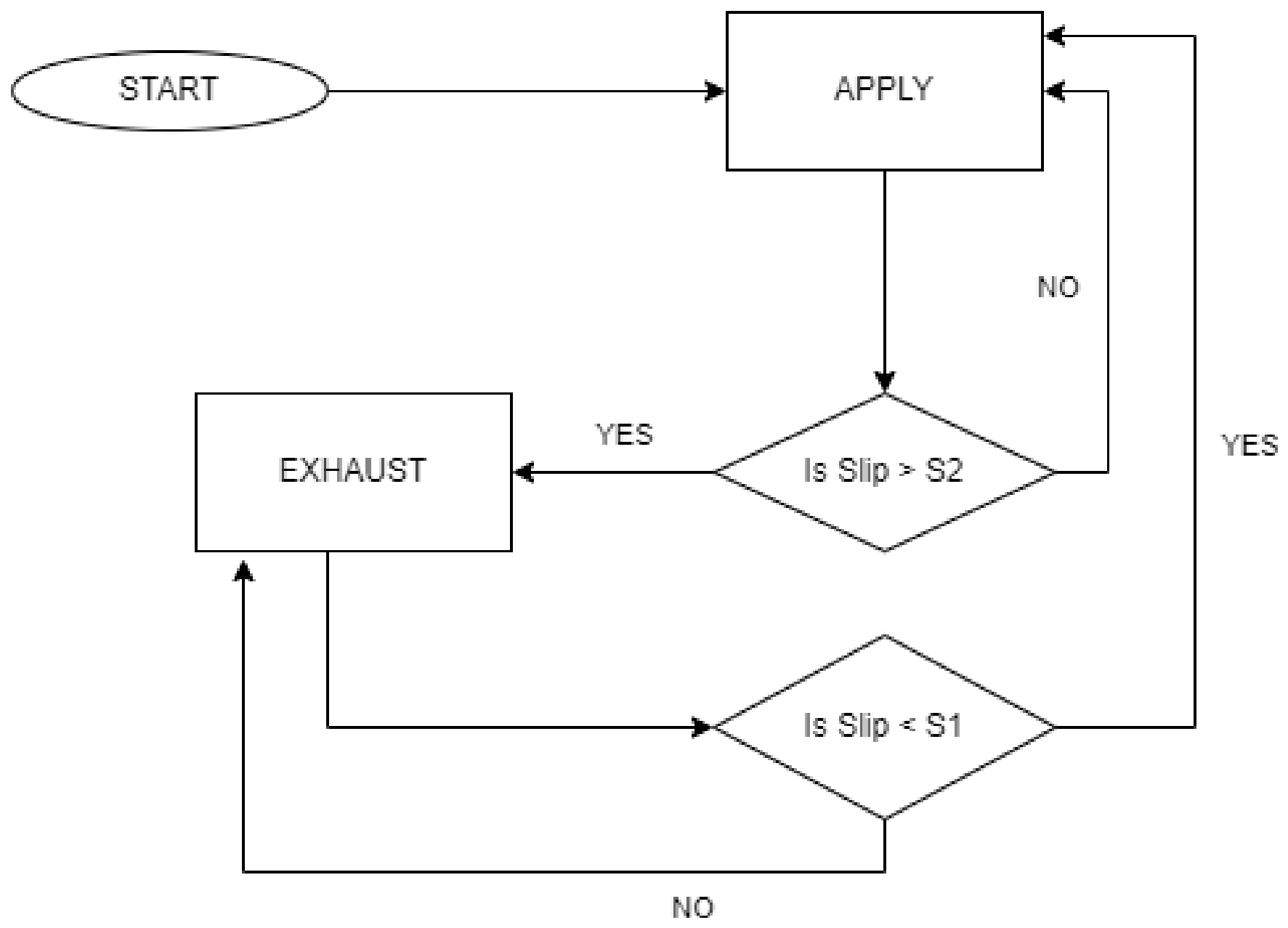
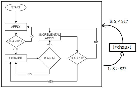
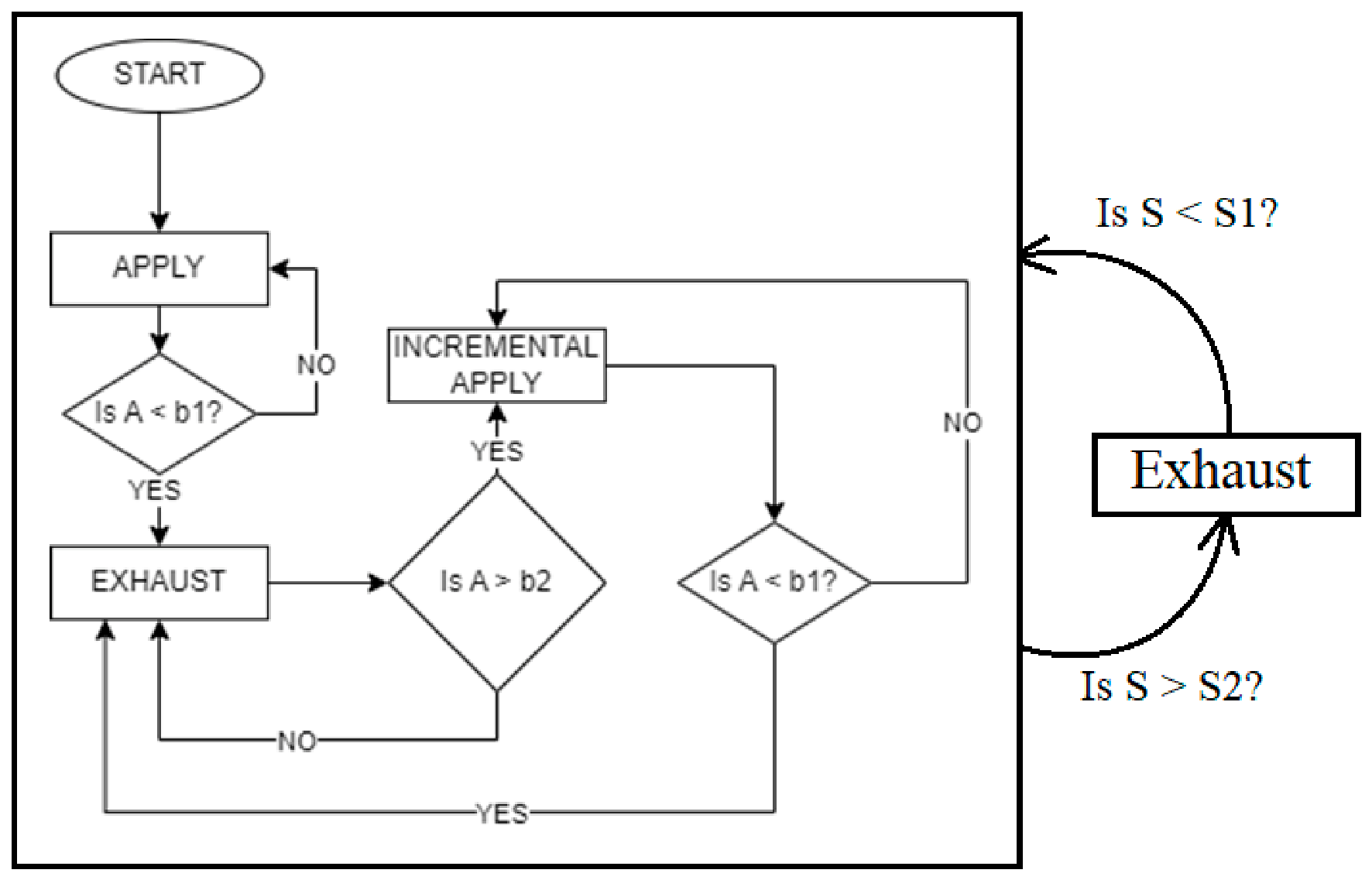
Two ABS controllers were considered during testing. Algorithm #1 is a slip-based controller. During braking, chamber pressure is increased while the estimated longitudinal slip remains below the upper slip threshold. When the slip exceeds the upper threshold, the controller commands pressure exhaust until the slip falls below the lower threshold. Pressure is then reapplied, producing an apply–exhaust cycling behavior governed primarily by the estimated slip state. ABS intervention is disabled below 10 km/h to avoid unstable low-speed slip estimation and unnecessary valve activity near standstill. The logic of ABS Algorithm #1 is given in Figure 19 below.

Figure 19. Slip-threshold pressure modulation logic used in Algorithm #1.

Algorithm #2 uses both wheel acceleration and longitudinal slip. In this strategy, pressure is initially applied until the wheel acceleration falls below the lower acceleration threshold, indicating rapid wheel deceleration and the onset of potential lock-up. The controller then commands pressure exhaust until the wheel acceleration recovers above the upper acceleration threshold. After recovery, a stepped-apply stage alternates pressure application and hold phases to rebuild braking pressure more gradually, rather than immediately returning to full pressure application. A slip override layer is added on top of the acceleration logic: when the estimated slip exceeds the upper slip threshold, the controller forces pressure exhaust; when slip decreases below the lower threshold, control is returned to the acceleration-based logic. The logic of ABS Algorithm #2 is given in Figure 20 below.

Figure 20. Wheel-acceleration and slip override logic used in Algorithm #2.

As both algorithms require a calculation of the wheel slip, a vehicle speed estimation algorithm is needed. The vehicle-speed estimator used for HIL and vehicle preparation was intentionally kept low in complexity. The fastest/slowest-wheel logic given in Section 2.2.4 was selected because it provided sufficient agreement with more complex speed-estimation candidates while being easier to implement in an embedded controller. During braking, the fastest wheel is less affected by excessive braking slip and therefore provides a conservative estimate of vehicle speed. During acceleration, the slowest wheel is less affected by drive slip and provides a more reliable reference.

2.6. ABS Reverse Engineering

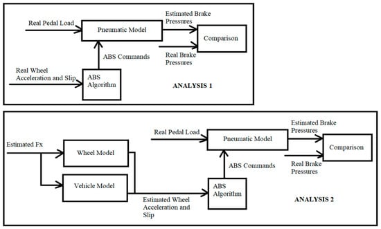
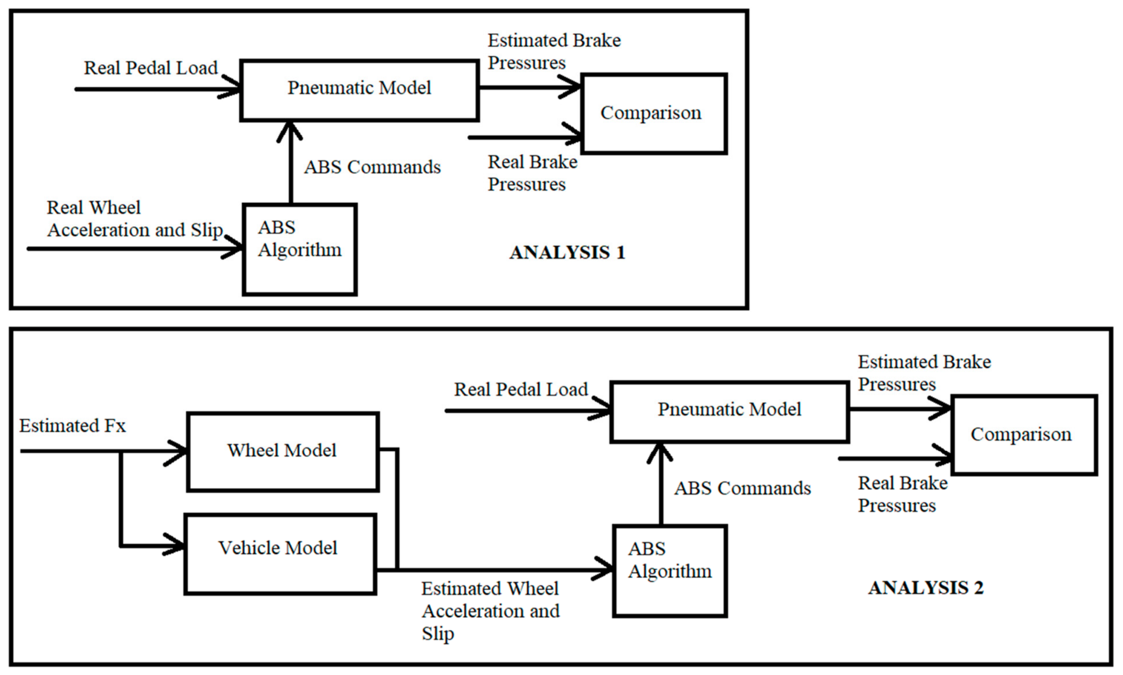
ABS reverse-engineering tests were then used to infer the switching behavior of a benchmark controller. The procedure is summarized in Figure 21. Here, the acceleration-based ABS algorithm described in Section 2.4 is used for the analysis and comparison.

Figure 21. Benchmark ABS reverse-engineering test used to infer threshold and timing behavior.

In the benchmark controller, ABS intervention is treated as a pressure-modulation process used to prevent wheel lock while keeping the tire near the useful region of the force–slip curve.

When excessive slip or large negative wheel acceleration indicates an approaching lock condition, the ABS modulator holds or exhausts brake pressure. Once the wheel recovers, pressure is reapplied. This apply–hold–exhaust sequence produces the characteristic pressure oscillations seen during ABS braking, especially in pneumatic heavy-vehicle systems where valve delays and chamber filling/exhausting dynamics affect the response.

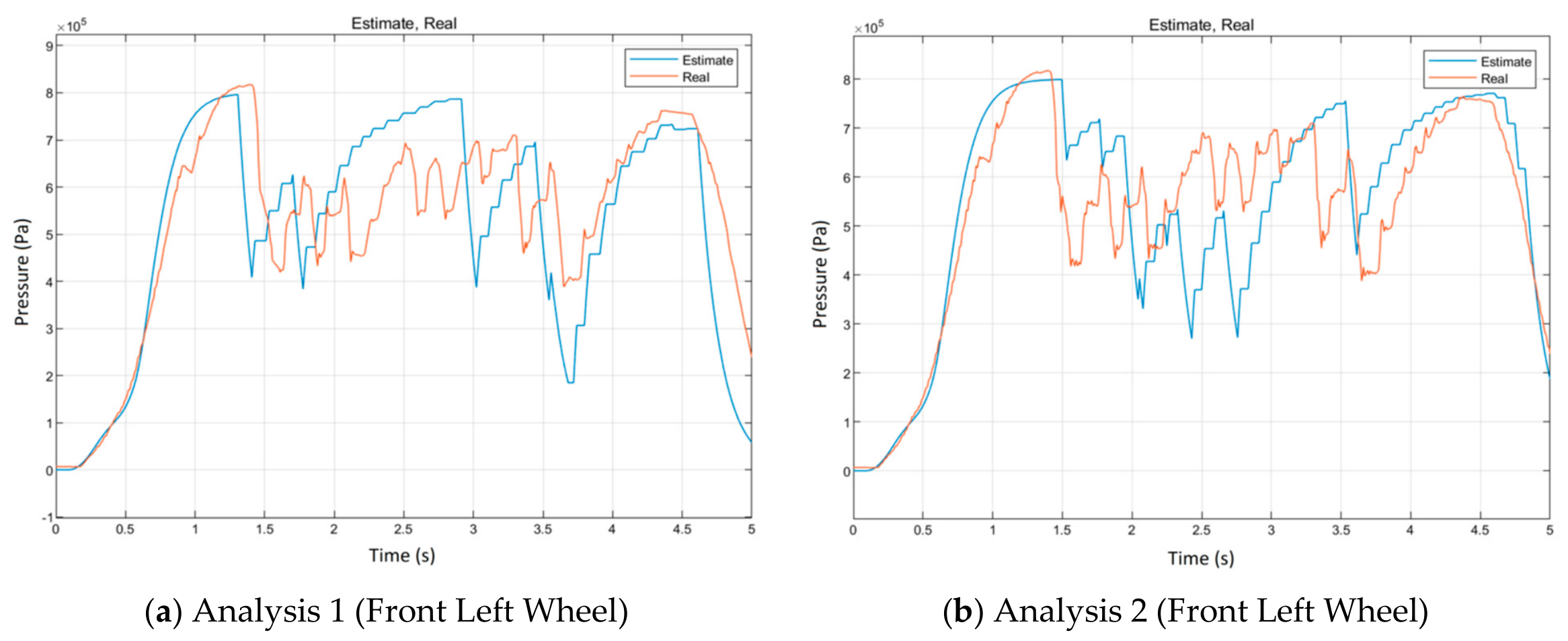
Two analyses were performed to separate the ABS logic from the plant-model behavior. In the first analysis, measured wheel acceleration and slip were supplied directly to the modeled ABS logic, and the resulting ABS commands were passed through the calibrated pneumatic model.

The estimated brake pressures were then compared with the measured chamber pressures, allowing the ABS threshold, switching sequence, and timing behavior to be evaluated. In the second analysis, the tire, wheel, and vehicle models were used to generate estimated wheel acceleration and slip.

These estimated states were then passed to the ABS logic and pneumatic model, allowing the complete simulation chain to be evaluated. This second path is more demanding because errors from tire-force estimation, vehicle dynamics, wheel dynamics, controller logic, and pneumatic response all appear in the final pressure comparison. Figure 22 below shows the outcomes of the comparisons for both scenarios.

Figure 22. Comparison of Real and Estimated Brake Pressures for (a) First braking analysis, and (b) the second braking analysis.

The reverse-engineering comparison showed that Algorithm #2 could reproduce the main modulation behavior observed from the benchmark WABCO^® ECU. In particular, the estimated pressure traces showed similar pressure build-up, hold/exhaust, and re-apply phases when the upper and lower wheel-acceleration thresholds were tuned appropriately. Therefore, the reverse-engineering process provided two outcomes. First, it gave a practical threshold range for Algorithm #2 by matching its switching behavior to the benchmark controller. Second, it provided an initial validation of the proposed ABS logic, since the algorithm was able to generate pressure-modulation commands with the same general dynamic behavior as the commercial ABS controller. Although exact pressure matching was not expected because of pneumatic delays, chamber dynamics, and model uncertainty, the comparison confirmed that the selected acceleration-based ABS structure was suitable for the following MIL, SIL, HIL, and vehicle validation stages.

2.7. Validation Scenarios

MIL, SIL and HIL validation covered high-mu straight braking, low-mu straight braking, split-mu straight braking, jump-mu straight braking, low-mu corner braking, high-mu corner braking and jump-mu corner braking.

The real-vehicle testing focused on longitudinal wet and dry asphalt braking with the custom ECU and comparison with a commercial WABCO^® ECU. The test-field limitations, however, prevented low-mu and split-mu testing.

3. Results

This Section provides the different results for simulation and real vehicle testing.

3.1. MIL and SIL Equivalence

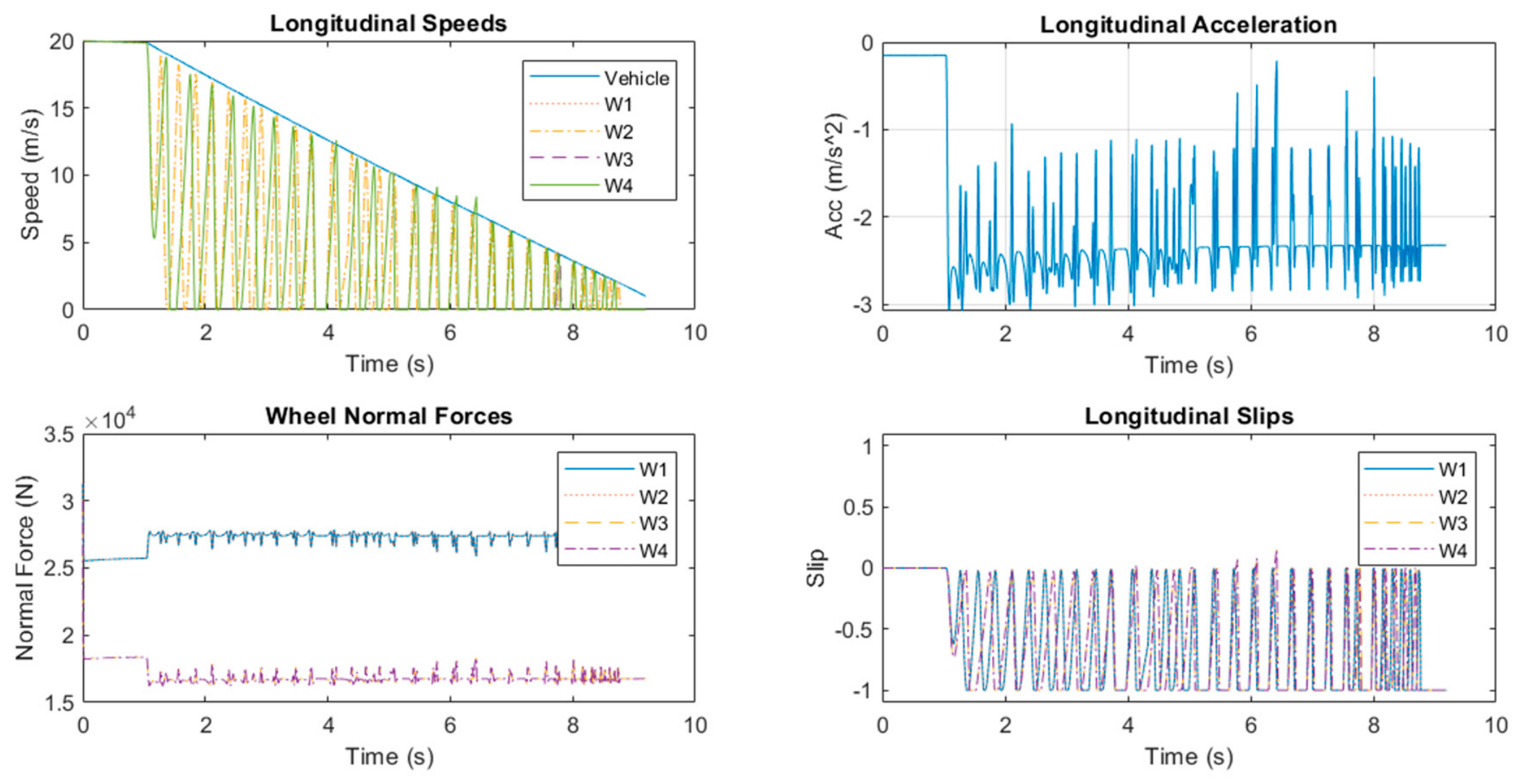
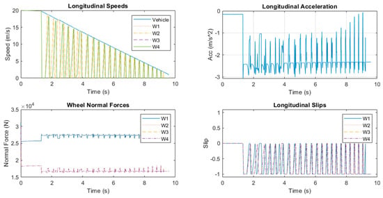
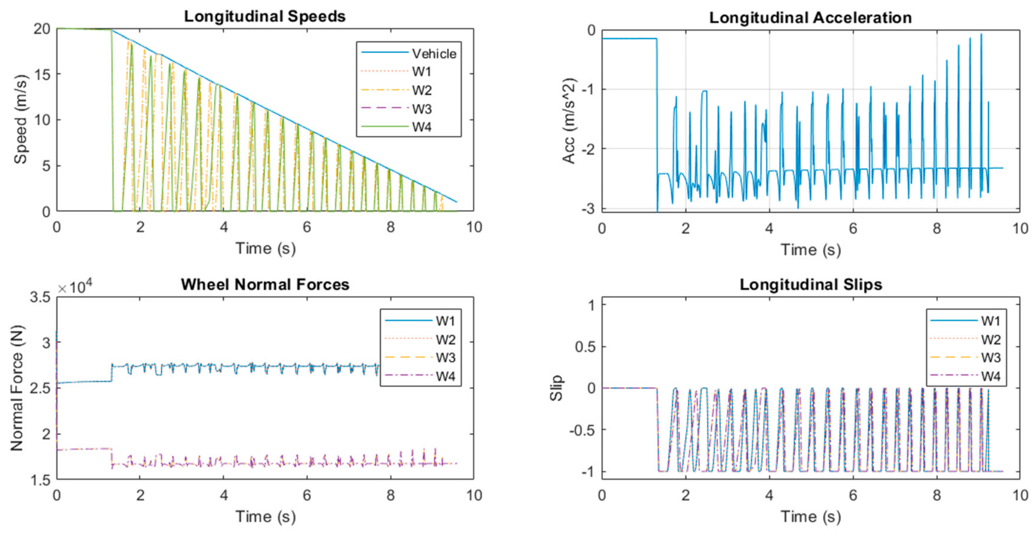
MIL and SIL simulations were compared to verify that the generated controller code reproduced the behavior of the original Simulink controller model. In the MIL configuration, the controller logic was executed directly as Simulink blocks. In the SIL configuration, the same controller was converted to generated code and executed against the same plant model. Therefore, close agreement between the two cases indicates that the code-generation step did not alter the intended ABS logic, timing sequence, or pressure-modulation decisions. The representative MIL and SIL results shown in Figure 23 and Figure 24 indicate that the generated-code implementation preserved the main controller response across the selected braking scenarios. Vehicle speed, wheel-speed evolution, brake-pressure cycling, and slip-regulation behavior followed the same trends in both environments.

Figure 23. MIL vehicle-response result for low-mu ABS braking.

Figure 24. SIL vehicle-response result for low-mu ABS braking.

This agreement was used as a prerequisite for moving the controller to HIL, where the physical ECU and real-time plant interface introduce additional timing, signal-conditioning, and I/O constraints.

3.2. HIL Validation

HIL testing extended the MIL/SIL validation by introducing the physical ECU, real-time execution constraints, I/O mapping, signal conditioning, and the pneumatic circuit. At this stage, the controller was executed on the ECU and coupled to the real-time TruckMaker^® vehicle model and physical pneumatic circuit.

Therefore, the HIL tests provided a more demanding intermediate validation step before vehicle implementation. Across the HIL scenarios, all candidate ABS strategies were able to decelerate the vehicle while maintaining overall stability.

Algorithm #1 produced acceptable braking performance in the simpler straight-line cases; however, it was more sensitive to excessive slip peaks because its main intervention logic depended on slip-threshold crossing.

Algorithm #2 showed the most balanced behavior in the HIL environment. By combining wheel-acceleration thresholds with a slip override layer, it responded earlier to imminent wheel lock while still preventing sustained high-slip operation.

Compared with Algorithm #1, Algorithm #2 maintained effective deceleration with fewer severe slip excursions and more consistent pressure recovery after exhaust events. Figure 25, Figure 26, Figure 27, Figure 28, Figure 29 and Figure 30 show the HIL results used for this comparison.

Figure 25. HIL result for Algorithm #1 during low-mu corner braking.

Figure 26. HIL result for Algorithm #1 during split-mu straight braking.

Figure 27. HIL result for Algorithm #1 during high-mu braking.

Figure 28. HIL result for Algorithm #2 during low-mu corner braking.

Figure 29. HIL result for Algorithm #2 during split-mu straight braking.

Figure 30. HIL result for Algorithm #2 during high-mu braking.

Figure 25, Figure 26 and Figure 27 present Algorithm #1 under low-mu corner braking, split-mu straight braking, and high-mu braking, respectively. Figure 28, Figure 29 and Figure 30 present the corresponding HIL results for Algorithm #2 under the same test conditions.

Table 10 below shows the results gathered from HIL testing.

Table 10. HIL Simulation Results Summary.

Quantity	Low Mu Algo #1	Split Mu Algo #1	High Mu Algo #1	Low Mu Algo #2	Split Mu Algo #2	High Mu Algo #2
Mean Initial Speed (km/h)	47.6	47.9	63.1	47.5	47.5	64.1
Standard Deviation (Initial Speed)	0.01	0.02	0.09	0.03	0.01	0.07
Mean Deceleration (m/s2)	2.29	2.33	4.51	2.38	2.57	4.53
Standard Deviation (Deceleration)	0.01	0.02	0.03	0.05	0.06	0.17
Mean Stopping Distance (m)	42.79	39.44	38.50	42.15	35.32	38.51
Standard Deviation (Stopping Distance)	0.80	0.21	0.38	0.90	0.66	1.52

Each HIL scenario was repeated three times, and the mean values and sample standard deviations were calculated to assess repeatability. The very small standard deviations in initial speed confirm that the repeated runs were performed under closely matched starting conditions. Deceleration results were also highly repeatable for Algorithm #1, with standard deviations between 0.015 and 0.025 m/s², while Algorithm #2 showed somewhat greater variability, particularly in the high-$\mu$ case (0.167 m/s²). Stopping-distance variability was generally limited, although the highest standard deviation occurred for Algorithm #2 under high-$\mu$ braking (1.526 m). In terms of mean performance, Algorithm #2 produced slightly greater deceleration and shorter stopping distances in the low-$\mu$ and split-$\mu$ scenarios, whereas both algorithms showed comparable results under high-$\mu$ braking. Overall, the repeated HIL tests indicate consistent controller behavior across the evaluated scenarios, with the largest variation observed for Algorithm #2.

3.3. Vehicle ABS Testing

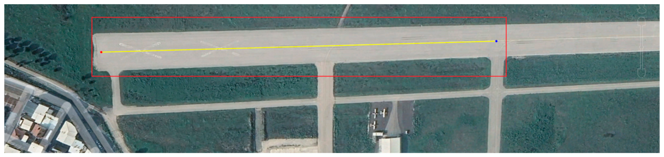
The real vehicle testing was carried out over two days, from 16 to 17 December 2025, on an approximately 400 m asphalt test section at the Bursa Yunuseli Airport, Türkiye. Braking tests were performed on both dry asphalt and wet asphalt. The real-vehicle testing was limited to dry- and wet-asphalt braking because the available test area, safety infrastructure, surface preparation capability, and project budget did not allow repeatable low-mu, split-mu, or jump-mu field testing with the heavy vehicle. Full-vehicle testing on controlled low-$\mu$, split-$\mu$, and jump-$\mu$ surfaces was not conducted because reproducing these conditions safely and repeatably for a heavy vehicle would have required specialized surface-preparation facilities, additional vehicle-recovery and containment measures, and expanded test-site safety infrastructure beyond the available project budget and the approved safety provisions of the test site. Therefore, these more demanding friction-transition and asymmetric-friction cases were evaluated in the MIL/SIL/HIL stages, while the vehicle tests were used to confirm controller transfer, ECU implementation, pressure modulation, wheel-lock prevention, and benchmark-level braking behavior under the available full-vehicle test conditions. The WABCO^® ECU was selected as the commercial benchmark because WABCO^® is a major supplier of commercial-vehicle ABS/EBS braking systems. In the European Commission WABCO^® decision, WABCO^® was reported to have an estimated 40–50% global share and 50–60% EEA share in commercial-vehicle ABS/EBS braking systems required for ADAS interaction [36]. Therefore, although the benchmark comparison is limited to one commercial ECU, the selected ECU represents an industrially relevant commercial ABS platform.

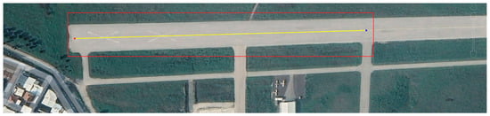
Figure 31 shows the test area and the road section used for the final braking campaign. The available straight asphalt section was approximately 400 m long and had an average slope of about 0.1%, which defined the practical limits on approach speed, braking distance, and test repeatability.

Figure 31. Bursa Yunuseli Airport test area (40°13′50.31278″ N, 29°0′40.94807″ E). The red area is the section of the runway used for testing. The yellow line indicates the path followed by the vehicle during testing.

Environmental conditions, road-surface condition, and the measured test-section profile were considered when interpreting the braking data.

Although low-mu, split-mu, and friction-transition maneuvers were considered, these cases could not be executed within the available test-area constraints. Therefore, the real-vehicle testing focused on wet- and dry-asphalt braking cases that could be repeated safely and consistently on the available test section.

The vehicle tests were used to evaluate the transfer of the developed ABS logic from the HIL environment to the physical vehicle, with emphasis on wheel-slip regulation, pressure-modulation behavior, longitudinal deceleration, and repeatability under measured road conditions.

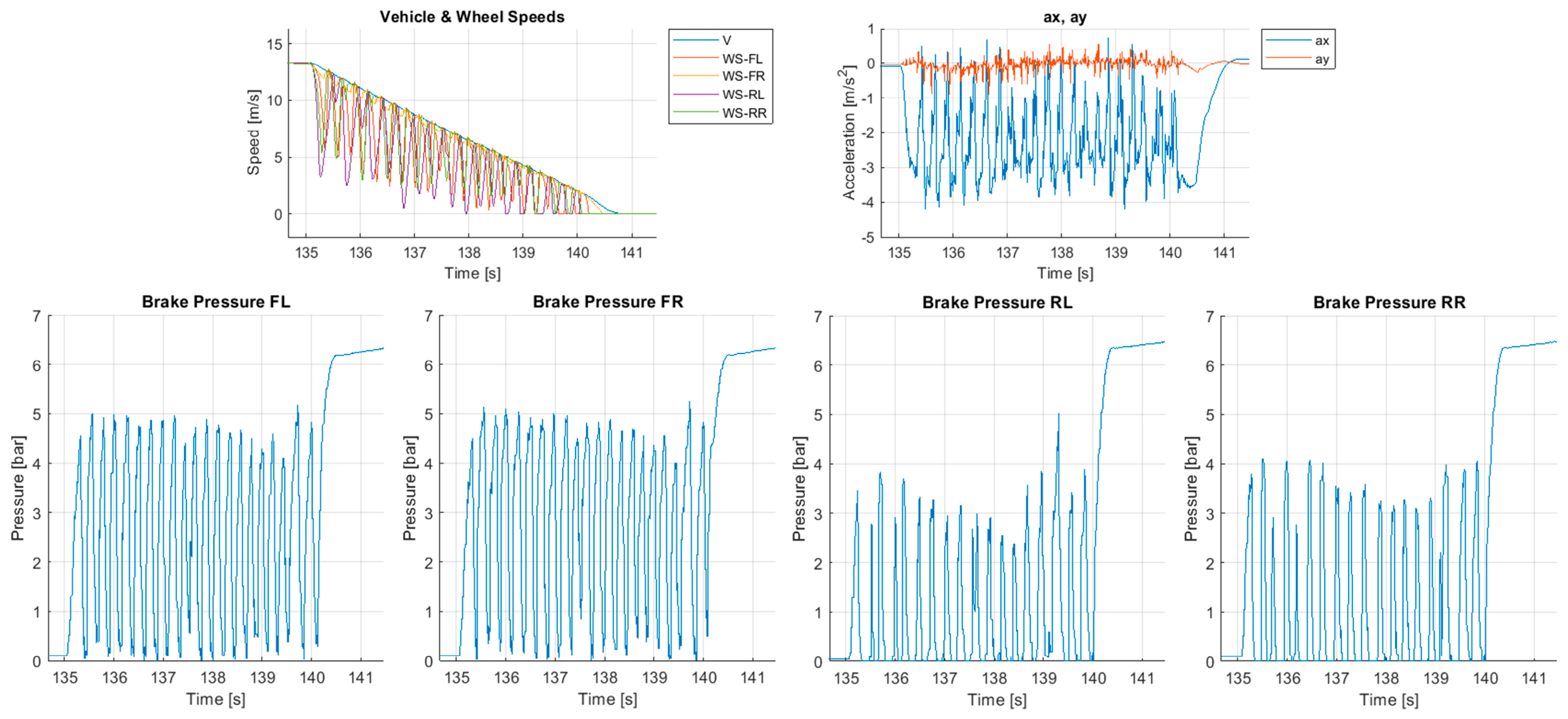
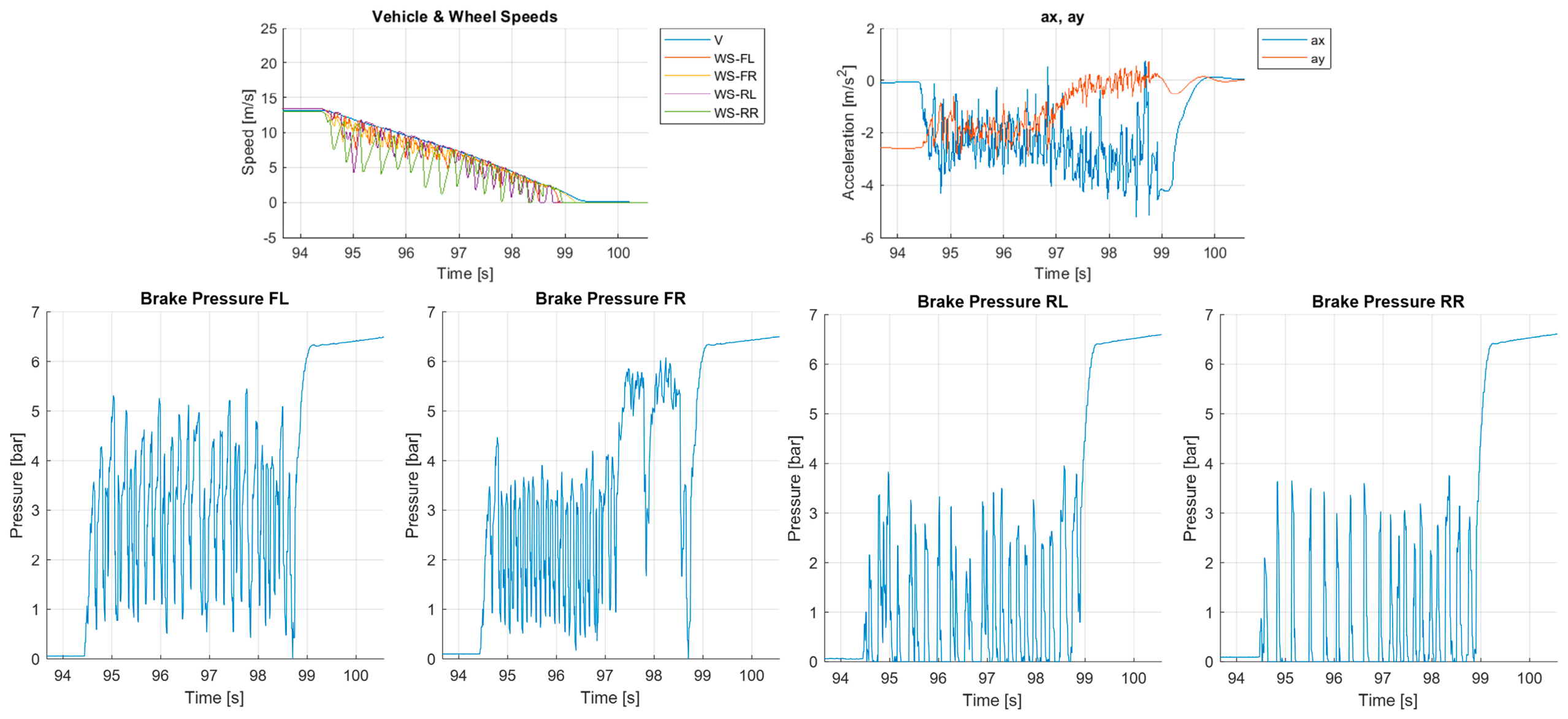
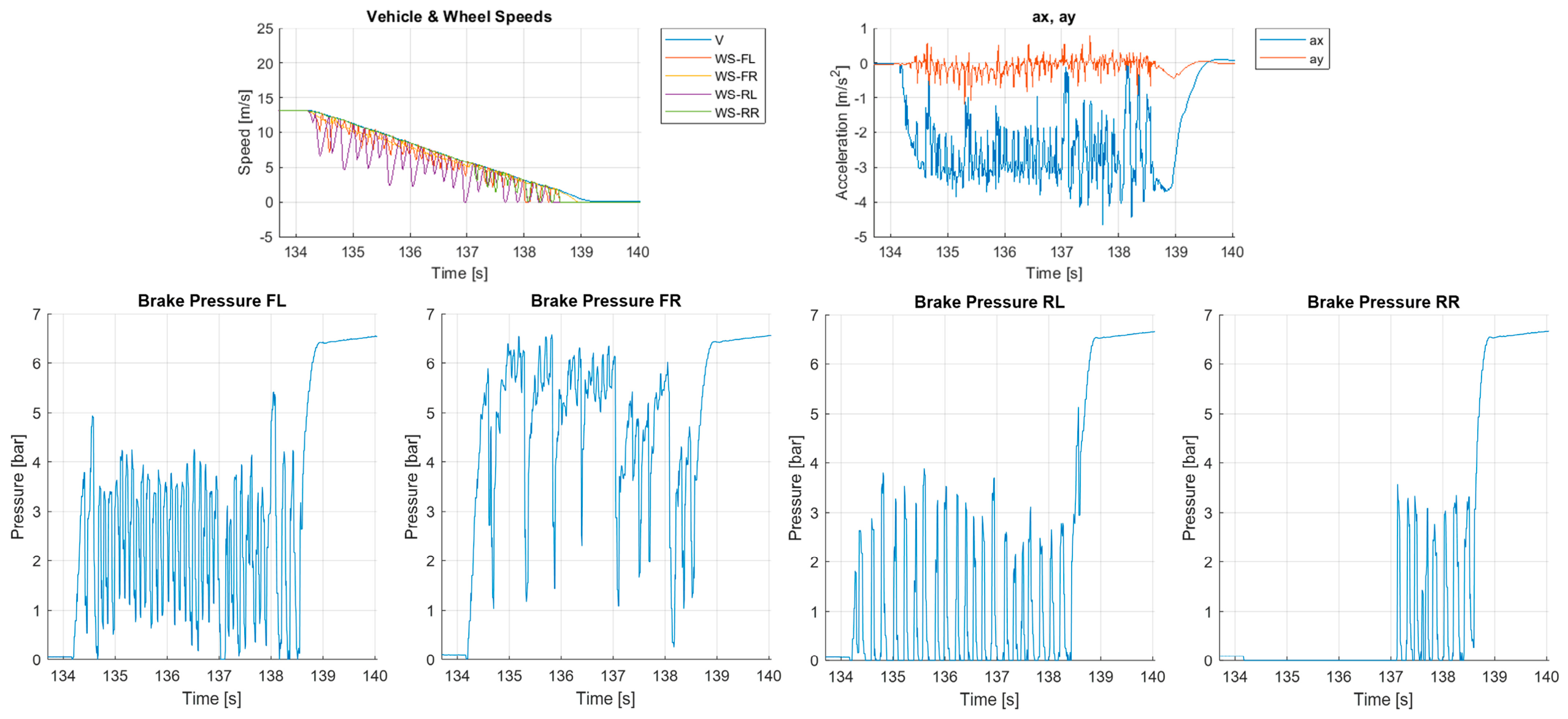
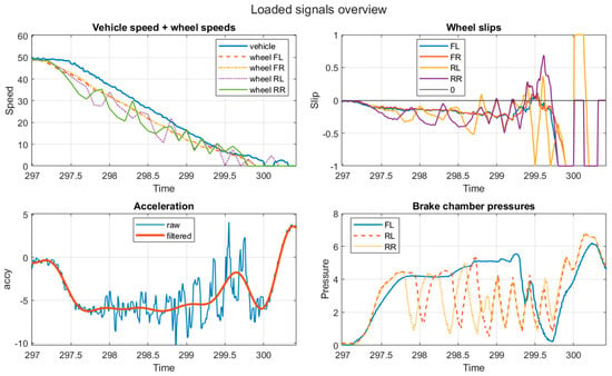
The WABCO^® ECU was used as a qualitative commercial reference during the vehicle-testing and calibration process. Based on observations by the test driver and engineering team, the developed controller exhibited the expected ABS intervention sequence and broadly comparable pressure-apply, hold, exhaust, and reapply behavior. At vehicle speeds below approximately 10 km/h, however, the developed controller produced more perceptible longitudinal jerk than the commercial ECU. This difference was attributed primarily to the stepped pressure-apply strategy used by the WABCO^® ECU, which enabled finer regulation of the pressure-build-up gradient, whereas Algorithm #1 did not include an equivalent stepped apply phase. In addition, near the end of the braking maneuver, the increasing magnitude of the calculated wheel slip as vehicle speed decreased caused Algorithm #1 to command excessive pressure exhaust. This reduced braking performance during the final stage of the stop and contributed to the greater jerk observed relative to the WABCO^® ECU. Nevertheless, the developed controller achieved the principal ABS objective of regulating wheel slip while maintaining stable braking behavior.

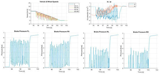
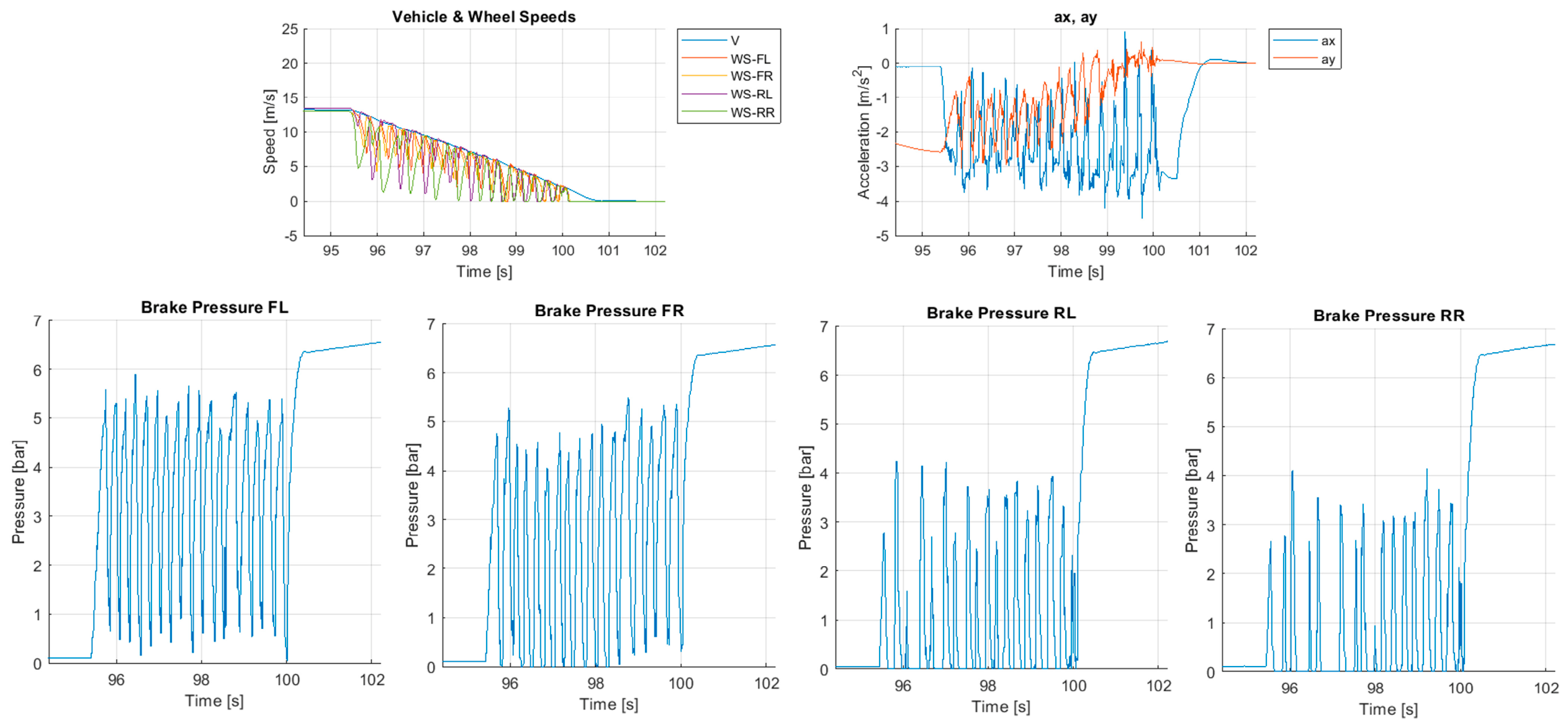
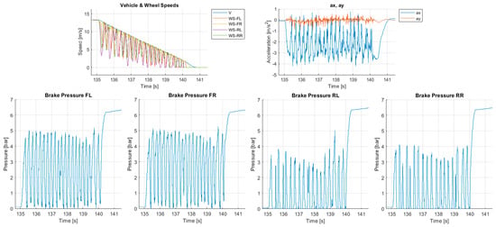
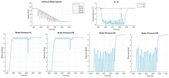
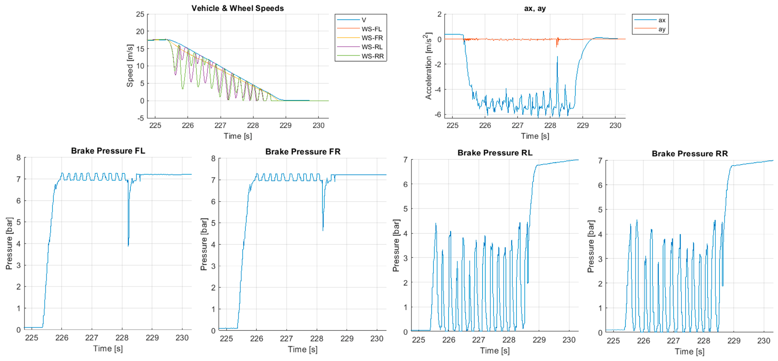
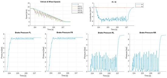
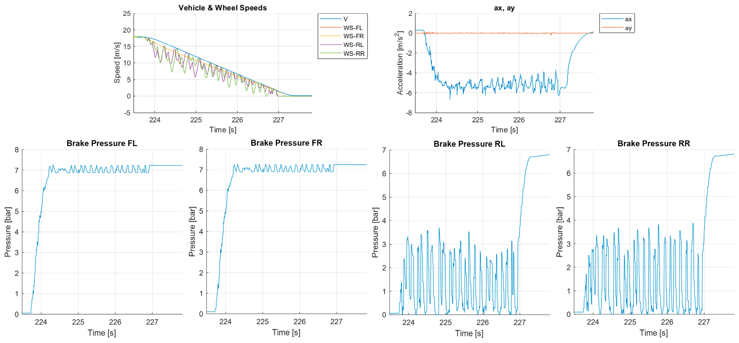
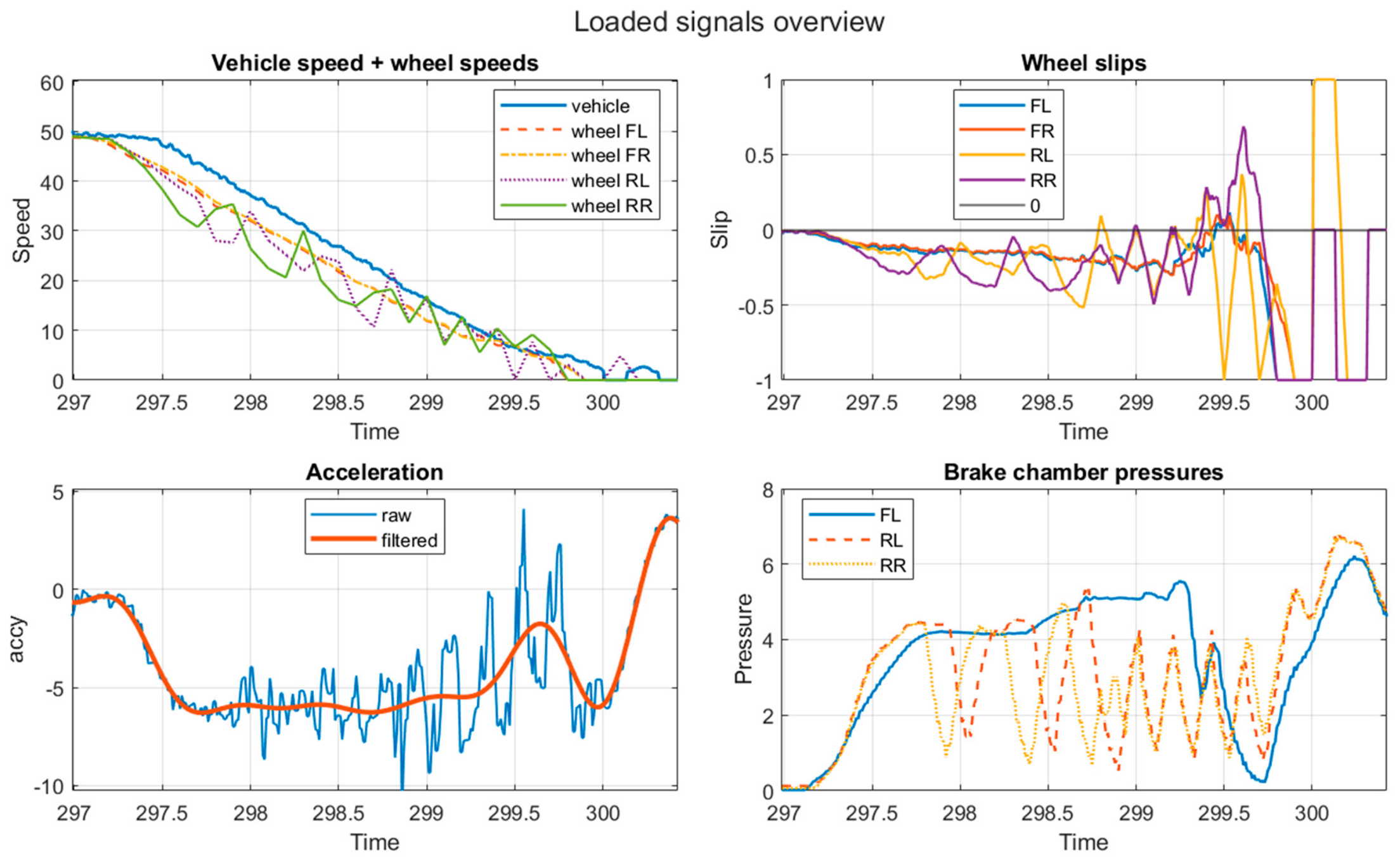
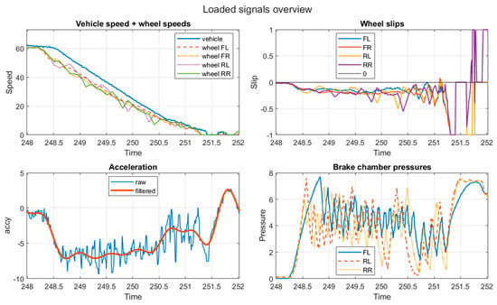
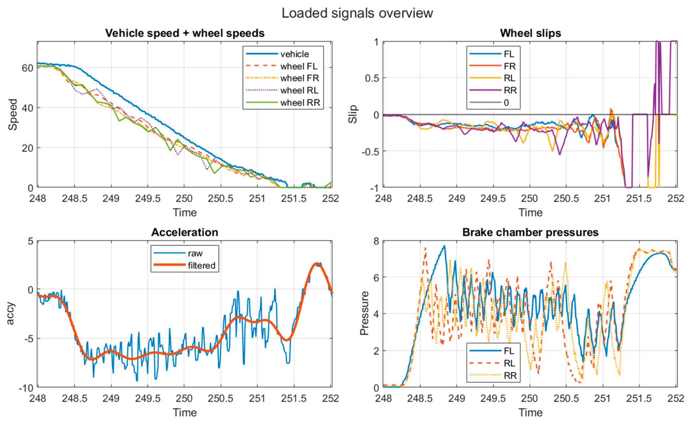
Figure 32 and Figure 33 show the real-vehicle braking results, including vehicle speed, wheel slip, longitudinal acceleration, brake pressure, and pedal-force. The results indicate that the controller responded consistently to the driver input, modulated chamber pressure during slip growth, and recovered braking pressure after exhaust phases. The measured deceleration, wheel-slip, and pressure trends confirmed stable ABS intervention and successful transfer of the developed controller from the HIL environment to the vehicle.

Figure 32. Real-vehicle braking data collected for Algorithm #1.

Figure 33. Real-vehicle braking data collected for Algorithm #2.

Overall, it was verified that the developed ABS could be implemented on the test vehicle and could deliver stable asphalt braking performance under the test conditions. Table 11 below shows the results of the real vehicle testing. It can be seen that both algorithms were able to provide satisfactory braking performance. The analysis for Algorithm #1 uses data from six runs, and for Algorithm #2 uses four runs.

Table 11. Summary of results for real vehicle testing.

Quantity	ABS Algorithm #1	ABS Algorithm #2
Mean Initial Speed (km/h)	49.9	59.7
Standard Deviation (Initial Speed)	0.84	0.92
Mean Deceleration (m/s2)	−4.20	−3.94
Standard Deviation (Deceleration)	0.42	0.47
Mean Stopping Distance (m)	21.65	26.24
Standard Deviation (Stopping Distance)	0.82	2.78

The repeated full-vehicle tests showed relatively consistent initial speeds within each algorithm, with standard deviations below 1 km/h. Algorithm #1 produced a mean deceleration magnitude of 4.20 m/s² and a mean stopping distance of 21.65 m, while Algorithm #2 produced 3.94 m/s² and 26.24 m, respectively. The larger stopping distance for Algorithm #2 should also be interpreted in relation to its higher mean initial test speed. Overall, the standard-deviation results indicate acceptable repeatability.

4. Discussion

The main outcome of the validation process was the progressive refinement of the ABS controller as it moved from simulation-based testing to real-vehicle evaluation. Across the MIL, SIL, HIL, and field-test stages, the controller was assessed not only in terms of stopping performance, but also with respect to signal robustness, calibration effort, pressure modulation stability, and repeatability under practical operating conditions.

During model-based validation, both controller structures were evaluated under different braking and road-friction conditions. The acceleration-assisted strategy provided useful information on rapid wheel-speed reduction and incipient lock-up tendencies, while the slip-based strategy provided a direct slip-regulation reference.

The HIL and reverse-engineering results were particularly useful for tuning the acceleration thresholds and slip override limits of Algorithm #2, since its pressure build-up, hold/exhaust, and re-apply behavior could be compared with the benchmark WABCO^® ECU. The real-vehicle tests then provided an additional validation stage for confirming that the developed ABS logic could be implemented on the physical vehicle and produce stable braking behavior.

The final vehicle-test calibration was selected based on the available test conditions, measurement setup, and repeatability of the braking runs. Under these conditions, the implemented controller produced stable pressure modulation, prevented sustained wheel lock, and provided repeatable braking performance. Qualitative observations by the test driver and engineering team indicated that its intervention sequence and general modulation character were consistent with those of the commercial reference controller, although the commercial ECU was perceived as smoother during some low-speed portions of the stop.

Experimental ABS studies using commercial WABCO^® braking hardware provide additional context for the present results. For example, [The test and simulation of ABS on rough, non-deformable terrains] reported a stopping distance of 34.04 m from 60 km/h on a smooth road using a vehicle equipped with a WABCO^® hydraulic modulator and a separately implemented Bosch-type ABS algorithm. Because the vehicle, braking architecture, controller implementation, and test conditions differ from those of the present study, this result is included only as a literature reference rather than as a direct quantitative benchmark.

The acceleration-assisted ABS structure remains an important part of the developed validation framework. The reverse-engineering and HIL results showed that the upper and lower wheel-acceleration thresholds could be tuned to reproduce the general apply, hold, exhaust, and reapply sequence observed during operation of the commercial reference controller. These results provide useful calibration references for Algorithm #2 and support its continued use in simulation and HIL-based ABS development. Future work can further refine the wheel-speed processing, acceleration filtering, and pressure re-apply strategy to improve the repeatability of acceleration-based ABS calibration across a wider range of test conditions.

There are a few limitations in the study. First, low-mu, split-mu, and jump-mu field tests could not be completed due to the available project budget, test-area conditions, and safety limitations for heavy-vehicle testing. Therefore, these cases remain validated at the MIL/SIL/HIL level rather than at the full-vehicle level. While this reduces the coverage of real vehicle testing, it does not invalidate the main objective of the study, which was to demonstrate the complete development and transfer of a pneumatic ABS controller from model-based simulation and HIL testing to real-vehicle implementation under the available dry- and wet-asphalt conditions. Future work will extend the vehicle-test campaign to low-mu, split-mu, and jump-mu surfaces when suitable test infrastructure and safety conditions are available. Second, as only one commercial ECU was used for comparison, it might be better to use several different commercial options for comparison.

5. Conclusions

This study presented a simulation-to-field validation workflow for a pneumatic ABS controller developed for a heavy vehicle. The workflow included parameter identification, MIL simulation, SIL code-equivalence testing, HIL validation, and final vehicle testing. The calibrated pneumatic, vehicle, and tire models reproduced the main braking characteristics required for controller development, while the MIL and SIL stages confirmed that the generated controller code preserved the intended control logic.

The validation process showed that ABS controller calibration must consider both simulated braking performance and real implementation behavior. The MIL, SIL, and HIL stages enabled the controller logic, threshold values, pneumatic response, and pressure-modulation behavior to be evaluated before vehicle testing. In particular, the acceleration-assisted Algorithm #2 was useful for identifying wheel-acceleration threshold ranges and reproducing benchmark-like modulation behavior in HIL. The vehicle tests then confirmed that the developed ABS controller could be implemented on the physical vehicle and could provide stable braking performance under the available wet- and dry-asphalt test conditions.

Algorithm #1 prevented sustained wheel lock during braking tests for the real vehicle. The developed controller produced stable and repeatable braking performance in the selected vehicle tests. Its general intervention and modulation characteristics were also assessed qualitatively by the test driver and engineering team against the commercial reference controller. The results also indicated that the algorithm could be successfully transferred from the simulation and HIL environment to the real vehicle.

The principal conclusion is therefore methodological as well as practical. ABS controller selection should not rely only on MIL, SIL, or idealized HIL results; it must also consider signal quality, ECU I/O behavior, filtering effects, pneumatic actuation dynamics, and repeatability in vehicle tests. Future work should expand the field-test envelope to low-mu and split-mu surfaces, improve wheel-speed acquisition and signal conditioning, introduce realistic sensor-noise and timing effects into HIL testing, and further refine pressure-recovery logic for smoother reapply behavior. These extensions would strengthen the validation basis and support further development of derivative-assisted control strategies without altering the main field-tested conclusion of this study.

References

- Limpert, R. Brake Design and Safety—Rudolf Limpert—Google Books. Available online: https://books.google.com.tr/books?hl=en&lr=&id=HXd0EAAAQBAJ&oi=fnd&pg=PA1&dq=Brake+Design+and+Safety&ots=uTs7K1rJ2I&sig=fvRe5KZLJ8hhx0h7sD5E-dbnqVA&redir_esc=y#v=onepage&q=Brake (accessed on 8 August 2023).
- Wong, J.Y. Theory of Ground Vehicle, 5th ed.; Wiley: Hoboken, NJ, USA, 2022. [Google Scholar] [CrossRef] [Scilit]
- EUR-Lex. 42016X0218(01)—EN—EUR-Lex. Available online: https://eur-lex.europa.eu/eli/reg/2016/194/oj/eng (accessed on 29 June 2026).
- Pacejka, H.B. Tire and Vehicle Dynamics. In Tire and Vehicle Dynamics, 3rd ed.; Elsevier: Amsterdam, The Netherlands, 2012; pp. 1–632. [Google Scholar] [CrossRef] [Scilit]
- Galip Ulsoy, A.; Peng, H.; Çakmakcı, M. Automotive Control Systems; Cambridge University Press: Cambridge, UK, 2012; ISBN 9781107010116. [Google Scholar] [CrossRef] [Scilit]
- Kiencke, U.; Nielsen, L. Automotive Control Systems: For Engine, Driveline, and Vehicle. Meas. Sci. Technol. 2000, 11, 1828. [Google Scholar] [CrossRef] [Scilit]
- Güleryüz, İ.C.; Başer, Ö. Modelling the longitudinal braking dynamics for heavy-duty vehicles. Proc. Inst. Mech. Eng. Part D J. Automob. Eng. 2021, 235, 2802–2817. [Google Scholar] [CrossRef] [Scilit]
- Miller, J.I.; Cebon, D. An investigation of the effects of pneumatic actuator design on slip control for heavy vehicles. Veh. Syst. Dyn. 2013, 51, 139–164. [Google Scholar] [CrossRef] [Scilit]
- Subramanian, S.C.; Darbha, S.; Rajagopal, K.R. Modeling the Pneumatic Subsystem of an S-cam Air Brake System. J. Dyn. Syst. Meas. Control 2004, 126, 36–46. [Google Scholar] [CrossRef] [Scilit]
- Aly, A.A. An Antilock-Braking Systems (ABS) Control: A Technical Review. Intell. Control Autom. 2011, 2, 186–195. [Google Scholar] [CrossRef]
- Austin, L.; Morrey, D. Recent advances in antilock braking systems and traction control systems. Proc. Inst. Mech. Eng. Part D J. Automob. Eng. 2000, 214, 625–638. [Google Scholar] [CrossRef] [Scilit]
- Hamamci, S.; Dousti, M.; Baslamısli, S.C.; Onder, E.T.; Solmaz, S. Design of a multiple-model switching controller for ABS braking dynamics. Trans. Inst. Meas. Control 2015, 37, 582–595. [Google Scholar] [CrossRef] [Scilit]
- Jiang, F.; Gao, Z. An Adaptive Nonlinear Filter Approach to the Vehicle Velocity Estimation for ABS. In Proceedings of the 2000. IEEE International Conference on Control Applications. Conference Proceedings (Cat. No.00CH37162), Anchorage, AK, USA, 27 September 2002; pp. 490–495. [Google Scholar] [CrossRef] [Scilit]
- Guo, H.; Cao, D.; Chen, H.; Lv, C.; Wang, H.; Yang, S. Vehicle dynamic state estimation: State of the art schemes and perspectives. IEEE/CAA J. Autom. Sin. 2018, 5, 418–431. [Google Scholar] [CrossRef] [Scilit]
- Singh, K.B.; Arat, M.A.; Taheri, S. Literature review and fundamental approaches for vehicle and tire state estimation. Veh. Syst. Dyn. 2019, 57, 1643–1665. [Google Scholar] [CrossRef] [Scilit]
- De Farias, A.B.C.; Rodrigues, R.S.; Murilo, A.; Lopes, R.V.; Avila, S. Low-cost hardware-in-the-loop platform for embedded control strategies simulation. IEEE Access 2019, 7, 111499–111512. [Google Scholar] [CrossRef] [Scilit]
- Salaani, M.K.; Rao, S.; Every, J.L.; Mikesell, D.R.; Barickman, F.; Elsasser, D.; Martin, J. Hardware-in-the-Loop Pneumatic Braking System for Heavy Truck Testing of Advanced Electronic Safety Interventions. SAE Int. J. Passeng. Cars-Mech. Syst. 2016, 9, 912–923. [Google Scholar] [CrossRef] [Scilit]
- Cheli, F.; Concas, A.; Giangiulio, E.; Sabbioni, E. A simplified ABS numerical model: Comparison with HIL and full scale experimental tests. Comput. Struct. 2008, 86, 1494–1502. [Google Scholar] [CrossRef] [Scilit]
- Li, S.; Zhao, J.; Yang, S.; Fan, H. Research on a coordinated cornering brake control of three-axle heavy vehicles based on hardware-in-loop test. IET Intell. Transp. Syst. 2019, 13, 905–914. [Google Scholar] [CrossRef] [Scilit]
- Baṣlamiṣli, S.Ç.; Köse, I.E.; Anlaş, G. Robust control of anti-lock brake system. Veh. Syst. Dyn. 2007, 45, 217–232. [Google Scholar] [CrossRef] [Scilit]
- Dousti, M.; Başlamişli, S.Ç. Experimental validation and robustness analysis of a multiple model switching antilock braking system control algorithm. Int. J. Veh. Des. 2016, 71, 226–257. [Google Scholar] [CrossRef] [Scilit]
- Savaresi, S.M.; Tanelli, M. Active Braking Control Systems Design for Vehicles; Springer Science & Business Media: Berlin/Heidelberg, Germany, 2010; Volume 53, Available online: https://books.google.com.tr/books?hl=en&lr=&id=MpVrZOWAyf4C&oi=fnd&pg=PR9&dq=Active+Braking+Control+Systems+Design+for+Vehicles&ots=emEy_zKvcO&sig=hKkw0_EZsDFwMI0ukYCvAZT4VHM&redir_esc=y#v=onepage&q&f=false (accessed on 27 July 2026).
- Savaresi, S.M.; Tanelli, M.; Cantoni, C. Mixed Slip-Deceleration Control in Automotive Braking Systems. J. Dyn. Syst. Meas. Control 2007, 129, 20–31. [Google Scholar] [CrossRef] [Scilit]
- Tanelli, M.; Sartori, R.; Savaresi, S.M. Combining Slip and Deceleration Control for Brake-by-wire Control Systems: A Sliding-mode Approach. Eur. J. Control 2007, 13, 593–611. [Google Scholar] [CrossRef] [Scilit]
- Tanelli, M.; Astolfi, A.; Savaresi, S.M. Robust nonlinear output feedback control for brake by wire control systems. Automatica 2008, 44, 1078–1087. [Google Scholar] [CrossRef] [Scilit]
- Pasillas-Lépine, W.; Loría, A.; Gerard, M. Design and experimental validation of a nonlinear wheel slip control algorithm. Automatica 2012, 48, 1852–1859. [Google Scholar] [CrossRef] [Scilit]
- Acarman, T.; Ozguner, U.; Hatipoglu, C.; Igusky, A.M. Pneumatic Brake System Modeling for Systems Analysis. In Proceedings of the International Truck & Bus Meeting & Exposition, Portland, OR, USA, 4 December 2000; SAE Technical Paper. [Google Scholar] [CrossRef] [Scilit]
- Hu, D.; Li, G.; Zhu, G.; Liu, Z.; Wang, Y. A Control-Oriented Linear Parameter-Varying Model of a Commercial Vehicle Air Brake System. Appl. Sci. 2020, 10, 4589. [Google Scholar] [CrossRef] [Scilit]
- Wei, L.; Wang, X.; Liu, H.; Li, L. System modeling, experimental validation and pressure estimation of the pneumatic braking system. Mech. Syst. Signal Process. 2023, 187, 109938. [Google Scholar] [CrossRef] [Scilit]
- Sridhar, N.; Devika, K.B.; Subramanian, S.C.; Vivekanandan, G.; Sivaram, S. Antilock brake algorithm for heavy commercial road vehicles with delay compensation and chattering mitigation. Veh. Syst. Dyn. 2021, 59, 526–546. [Google Scholar] [CrossRef] [Scilit]
- Tanelli, M.; Savaresi, S.M.; Cantoni, C. Longitudinal vehicle speed estimation for traction and braking control systems. In Proceedings of the 2006 IEEE Conference on Computer Aided Control System Design, 2006 IEEE International Conference on Control Applications, 2006 IEEE International Symposium on Intelligent Control, Munich, Germany, 4–6 October 2006; pp. 2790–2795. [Google Scholar] [CrossRef] [Scilit]
- Ashby, R.M. Hardware in the Loop Simulation of a Heavy Truck Braking System and Vehicle Control System Design. Master’s Thesis, The Ohio State University, Columbus, OH, USA, 2013. [Google Scholar]
- Xu, J.; Li, L.; Zhao, R.; Deng, F.; Li, G. A Rapid Verification System for Automatic Emergency Braking Control Algorithm of Passenger Car. Appl. Sci. 2023, 13, 508. [Google Scholar] [CrossRef] [Scilit]
- Riedemann, H.; Stanusch, G.; Tha, I.; Wolf, T. Method for Correcting a Vehicle Reference Speed. U.S. Patent No. 6,224,171, 1 May 2001. [Google Scholar]
- Lee, A.J.; Headley, P.M. ABS Reference Speed Determination. U.S. Patent 4,989,923, 5 February 1991. [Google Scholar]
- European Commission. Case M.9383—ZF/WABCO: Commission Decision Pursuant to Article 6(1)(b) of Council Regulation No 139/2004 and Article 57 of the Agreement on the European Economic Area; C(2020) 467 final; European Commission: Brussels, Belgium, 2020; CELEX No. 32020M9383. Available online: https://ec.europa.eu/competition/mergers/cases1/20212/m9383_1030_3.pdf (accessed on 29 July 2026).
Disclaimer/Publisher’s Note: The statements, opinions and data contained in all publications are solely those of the individual author(s) and contributor(s) and not of MDPI and/or the editor(s). MDPI and/or the editor(s) disclaim responsibility for any injury to people or property resulting from any ideas, methods, instructions or products referred to in the content. |
© 2026 by the authors. Licensee MDPI, Basel, Switzerland. This article is an open access article distributed under the terms and conditions of the Creative Commons Attribution (CC BY) license.