


Abstract
Strong broadband noise can mask the weak impact responses produced by bearing faults, while wavelet reconstructions selected only by signal-domain scores may not provide useful inputs for diagnosis. To address this problem, this paper presents WPMSR-1D-ResNet, a training-aware wavelet-domain controlled-noise augmentation framework. PKPM-guided particle swarm optimization first generates scale-specific perturbation candidates in the DWT detail coefficients. Signal-fidelity constraints remove distorted reconstructions, and a proxy CNN with identity fallback selects a global candidate according to validation Macro-F1. The final 1D-ResNet is trained jointly with the measured waveform and the selected augmented view, whereas inference uses only the raw signal. Under one fixed data construction and a common fixed 20-epoch budget, WPMSR-1D-ResNet achieved Macro-F1 at the predefined CWRU low-SNR endpoint and ranked third among eleven methods, placing it within the leading statistical group. Its paired mean exceeded raw-signal 1D-ResNet and per-slice PKPM replacement by 0.05582 and 0.05227, respectively, with gains in nine of ten paired computational seeds. Mixed-SNR training increased mean Macro-F1 across eight mismatched-noise conditions from to . The method ranked second on PU and third on acquisition-held-out AT data; on AT, it reduced the normal-state false-alarm rate from 0.2854 to 0.1646 while maintaining 0.9708 fault sensitivity. Raw-only inference required 0.266 ms per slice. WPMSR-1D-ResNet, therefore, aligns wavelet augmentation with diagnostic performance, preserves useful waveform information, and removes wavelet reconstruction and PSO from the deployment path.
1. Introduction
Rolling-element bearings are key components in rotating machinery, and their degradation can reduce equipment efficiency, interrupt production, and lead to secondary mechanical damage. Vibration-based diagnosis is widely used because local defects on the inner race, outer race, or rolling element produce impact responses that can be captured by accelerometers [1]. Randall and Antoni summarized the diagnostic mechanisms and practical signal features of rolling-element bearings in a tutorial review [2]. In practice, these impact components are often weak. They are mixed with shaft rotation, structural resonance, load-dependent background vibration, and sensor noise. The difficulty becomes more visible when a model trained under one operating load is tested under another load, as in the CWRU load-transfer setting [3]. Later CWRU-based reviews also showed how sensitive reported diagnostic performance can be to dataset construction and protocol choices [4]. Similar interference appears in the PU bearing dataset, where damage type and operating condition jointly affect the measured signal segments [5]. Therefore, preprocessing that can expose weak fault evidence before classification remains important for bearing fault diagnosis.
Existing studies have improved bearing diagnosis from both signal-processing and learning-based directions. Early neural diagnosis studies used time-domain features and wavelet preprocessing before classification [6,7]. Classical stochastic resonance was originally proposed as a noise-assisted mechanism [8], and later machinery-diagnosis studies developed adaptive cascade resonance [9], second-order noise-controlled resonance [10], sliding-window resonance detectors [11], time-delayed monostable resonance with deconvolution [12], stable-state matching for underdamped systems [13], adaptive unsaturated bistable resonance [14], and multiscale resonance spectrograms [15]. Review articles have summarized bearing signal processing [16], stochastic resonance in rotating machinery [17], and machinery fault detection applications [18]. Related work has also studied gearbox monitoring [19], frequency-shift multiscale tuning [20], coupled bistable resonance [21], multistability in signal processing [22], statistical-complexity features under variable speed [23], edge computing for machine signal processing [24], and recent noise-aided nonlinear feature extraction [25].
Deep neural networks then learned diagnostic features from raw or transformed vibration slices [26]. Representative classifiers include TICNN [27], residual learning [28], residual diagnosis networks [29], dynamically weighted wavelet residual networks [30], and residual shrinkage networks [31]. Recent work has extended this line in several directions. Spirto et al. used symmetrized-dot-pattern indices and a feedforward network for efficient bearing-fault detection on two public datasets [32]. Chen et al. embedded learnable wavelet kernels in a convolutional LSTM to combine interpretable spatial features with temporal modeling under noisy and nonstationary conditions [33]. Kulevome et al. developed analytic-wavelet data augmentation for bearing time series and evaluated it under reduced training data and low SNR [34]. Liu et al. combined adaptive stochastic-resonance preprocessing with CNN diagnosis for incipient faint faults [35]. Xu et al. designed a lightweight time-frequency Transformer for noise-robust bearing diagnosis and deployable inference [36]. Makrouf et al. combined continuous-wavelet multi-sensor fusion with transfer learning under variable-speed bearing conditions [37]. Alhams et al. evaluated ensemble classifiers on a dual-machine experimental bearing benchmark and analyzed feature importance across operating settings [38]. Sun et al. used wavelet-packet decomposition within an autoregressive generation scheme for imbalanced bearing data [39]. Zhao et al. compared diffusion-based augmentation with conventional generative alternatives for intelligent machine diagnosis [40]. Ping et al. combined synchrosqueezed wavelet representations with denoising diffusion augmentation for few-shot aero-engine bearing diagnosis [41]. Qin et al. developed a learnable wavelet-driven network that links variable-speed diagnosis with physically interpretable features [42].
Transfer-learning and domain-adaptation methods address changes between source and target conditions. Representative approaches include deep transfer learning [43], Wasserstein adversarial transfer learning [44], and the target-unlabeled A2CNN used as a separate comparator in this study [45]. Recent reviews organize the assumptions, datasets, and evaluation practices of bearing and rotating-machinery transfer diagnosis [46,47]. A formal survey and open comparison of unsupervised transfer methods provides a reproducible reference for target-domain adaptation [48]. Open-source benchmarking has likewise shown that data splits, input representations, and augmentation choices materially affect rotating-machinery results [49]. Xiao et al. recently reviewed domain-generalization assumptions and benchmarked representative methods for rotating machinery [50]. Zhang et al. used dual disentanglement to separate domain-related and fault-related information under unseen operating conditions [51]. These advances show that both preprocessing and model design matter, but they leave a narrower practical issue for preprocessing-based diagnosis. Many enhancement methods still require a known fault-frequency band, manual parameter selection, or a validation protocol that does not clearly connect signal transformation with stable classifier performance.
This study addresses low-SNR bearing diagnosis when the informative frequency band is not known in advance. Directly replacing every input with a signal-score-optimized reconstruction can misalign enhancement with the classification objective, move sample-wise optimization into inference, and discard useful information from the original waveform. WPMSR-1D-ResNet addresses these limitations by moving wavelet candidate search into training, selecting candidates according to downstream diagnostic performance, and retaining the raw signal as the learning and inference anchor. In this study, WPMSR denotes the resulting wavelet-domain controlled-noise augmentation module.
WPMSR-1D-ResNet follows a unified processing sequence. PKPM- guided PSO first generates a small set of global detail-scale candidates from the inner-training block. Correlation, normalized reconstruction error, and perturbation-energy constraints remove candidates that change the signal too strongly. A proxy CNN then ranks the remaining candidates by inner-validation Macro-F1, and a proxy-based identity fallback retains the raw mapping when no non-identity candidate reaches the predefined validation threshold. The final 1D-ResNet learns jointly from raw and selected WPMSR views and uses only raw slices during inference.
This study makes four contributions.
- We introduce WPMSR-1D-ResNet, which reformulates wavelet enhancement as diagnosis-aware training augmentation rather than direct test-signal replacement. This formulation jointly addresses score–task mismatch, sample-wise optimization cost, and the loss of useful waveform information.
- We design a constrained global candidate-selection mechanism that combines PKPM-guided PSO, signal-fidelity screening, proxy-CNN validation, and identity fallback. It links scale-specific wavelet perturbations to downstream diagnostic performance while preserving physically meaningful fault-frequency components.
- We develop raw-anchored dual-view learning to separate offline augmentation from online diagnosis. The classifier learns from measured and selected views during training but uses the raw-signal 1D-ResNet path during deployment, eliminating DWT reconstruction and test-time PSO.
- We establish a unified fixed-budget evaluation across five SNR levels, ten paired seeds, eleven competing methods, temporal-block shifts, mismatched noise, equal-budget search, component analysis, fault-frequency verification, and file-held-out PU and AT experiments. The resulting evidence shows gains over Raw and per-slice PKPM replacement, improved noise-mismatch performance, reduced AT false alarms, and low-latency raw-only inference.
The remainder of this paper is organized as follows. Section 2 defines the diagnostic task and wavelet representation. Section 3 presents WPMSR-1D-ResNet, including PKPM-guided candidate generation, proxy-based selection, and raw-anchored training. Section 4 describes the 1D-ResNet classifier. Section 5 reports the experiments, Section 6 discusses the findings, practical implications, and scope, and Section 7 concludes the paper.
2. Preliminaries and Problem Definition
2.1. Problem Setting
Let be a standardized vibration slice and its class label. Each raw record is divided into disjoint training, inner-validation, and test blocks before slicing, noise addition, or wavelet processing. The training and inner-validation blocks may be used to generate and select a wavelet-domain perturbation, while the test block is excluded from candidate generation, candidate selection, and classifier training.
A classifier is learned from a raw training view and a controlled wavelet-domain view . No prespecified fault-frequency band is required by the transformation. Its parameter contains the wavelet-noise scale and the detail-coefficient weight vector. Candidate settings are generated from inner-training signals and are selected according to inner-validation Macro-F1. The test interface is
so no WPMSR or PSO operation is performed on the test slice.
2.2. Wavelet Representation
Each slice is standardized as
For a level-L DWT, the standardized slice and an equal-length Gaussian-noise sequence are represented as
The approximation coefficient is retained and only the detail coefficients are perturbed
The recovered slice is . In the fixed protocol, db4 is used with and normalized-unit Gaussian noise with , and . PyWavelets 1.8.0 performs the transform in float64 precision with symmetric boundary extension. For a 2048-point slice, the coefficient lengths in the order are . Inverse DWT output is cropped to the original 2048 samples. The coefficient index and weight index use the same coarse-to-fine order, so .
Figure 1 illustrates the coefficient flow used by the WPMSR module and distinguishes the retained approximation coefficient from the perturbed detail coefficients.
Figure 1.
DWT decomposition used by WPMSR. Solid black arrows show the decomposition flow, red dashed arrows map the coefficients to the reconstruction groups, and the dashed red and green boxes identify the retained approximation and perturbed detail coefficients, respectively. Three levels are drawn for clarity; all experiments use db4 with six levels, preserve , and perturb only the detail coefficients. The supplied figure is a vector PDF and remains resolution independent.
3. Proposed Method
3.1. WPMSR-1D-ResNet Overview
WPMSR-1D-ResNet combines training-time wavelet-domain controlled-noise augmentation with a 1D residual classifier. Its WPMSR module first builds a candidate pool from the inner-training block. This pool contains the identity mapping, fixed detail-coefficient weights, and global candidates generated by PKPM-guided PSO. A small proxy CNN evaluates every candidate on three inner-validation folds. A non-identity candidate is accepted only when it passes the signal-fidelity constraints and the proxy-based selection rule. Identity remains an eligible fallback. Once selected, the candidate supplies a second training view for the final 1D-ResNet. Raw slices remain present throughout training and constitute the only input at inference. WPMSR denotes this wavelet-domain controlled-noise augmentation module, in which PKPM-guided PSO searches bounded perturbations of the DWT detail coefficients and downstream validation determines the training view.
This sequence gives each component one role. PKPM guides candidate generation, PSO searches the scale weights, the proxy CNN connects selection to the diagnostic objective, the identity fallback retains the unmodified option, and the raw anchor preserves the original diagnostic view. PKPM-guided PSO, therefore, describes an internal WPMSR operation rather than a separate diagnostic model.
Figure 2 summarizes the complete training and inference paths. Candidate generation, fidelity screening, proxy-CNN validation, and the identity fallback use only the training and validation data. The selected WPMSR view is combined with the raw view during joint training, whereas inference sends only the raw view to the trained 1D-ResNet.
Figure 2.
End-to-end WPMSR-1D-ResNet workflow. Solid black arrows show training and data flow, the dotted blue path shows raw-only inference, and the dashed boundary encloses operations restricted to training and validation data. Joint training uses the raw and selected WPMSR views, while inference uses the raw view only.
3.2. PKPM-Guided Global Candidate Generation
Candidate generation uses an equal number of inner-training slices from every class. For a candidate weight vector , the PKPM score is calculated from the original and reconstructed slices. The implementation calls SciPy’s welch function with a Hamming window, nperseg = N, the default nominal overlap of , constant detrending, an N-point FFT, one-sided output, and density scaling. Because the segment length equals the slice length, only one segment is available; the estimator is, therefore, a single-segment Hamming-windowed periodogram rather than a multi-segment Welch average. Let R be detected from . Specifically, local maxima above are detected, and R is the union of those peak bins and five neighboring bins on each side, clipped at the spectrum boundaries. If no peak is detected, R contains all spectrum bins. The same R is then used to compute the before- and after-transformation peak-region energies. This common reference prevents the numerator from moving to a different set of peaks after perturbation. The peak-region term is
All numerical denominators are lower-bounded by , the float64 machine epsilon. Time-domain kurtosis is
and dominant-peak enhancement is
The mean-intensity-gain penalty uses and
The balanced profile is
with . The four terms measure spectral peak-region change, impulsiveness, dominant-peak change, and mean-amplitude preservation, respectively. Their units and ranges differ, so the weights are treated as engineering profiles rather than theoretically optimal coefficients. Table 1 lists the five profiles fixed before the final test runs. The eight profile–scale specifications used for PSO are (balanced, 0.01), (balanced, 0.025), (balanced, 0.05), (balanced, 0.075), (spectral, 0.05), (peak, 0.05), (shape, 0.05), and (MIG-heavy, 0.05). Candidate selection compares their downstream validation performance instead of assuming that the balanced profile is universally best.
Table 1.
Prespecified PKPM weight profiles.
PKPM candidates must satisfy
For candidate c and inner-training slice i, denotes the PKPM score. For a profile with weights , the identity score is . Candidate-specific normalization uses the robust scale
and the PSO fitness is
where is the proportion of slices that violate Equation (10). The candidate-specific scaling is retained for exact agreement with the executed implementation. Subtracting the identity score expresses candidate improvement relative to the unmodified signal, while the median and MAD reduce the influence of isolated slices. The floor prevents a nearly constant candidate from receiving an arbitrarily large standardized value. Comparisons with pooled scaling, no scaling, alternative profiles, values, peak thresholds, and a multi-segment Welch estimate are reported in Appendix Table A12.
PSO uses 12 particles, 25 update iterations after the initial population evaluation, and at most five retained candidates per profile–scale specification. Positions are initialized uniformly on , velocities uniformly on , and the fixed coefficients are and . Velocity is clipped to in every dimension, position is clipped to , and the search stops after the fixed iteration budget. For particle i, the update is
where and the particle dimension is L.
For each SNR–seed setting, candidate generation examines four fixed candidates and five PSO outputs for each of eight profile–scale specifications. The fidelity screen is first applied to a balanced subset containing four slices per class. One feasible PSO candidate per specification is then retained, so the proxy evaluates 13 candidates in total: identity, four fixed candidates, and eight PKPM-guided PSO candidates.
Figure 3 summarizes the PKPM-guided PSO search and the reconstruction of a candidate WPMSR training view.
Figure 3.
PKPM-guided PSO search for detail-scale perturbation weights within WPMSR. The approximation coefficient remains unchanged. Solid black arrows show the particle-update sequence, dashed black paths carry coefficients and fitness information, and blue arrows denote DWT and inverse-DWT operations. The superscript ∗ identifies the global-best weight vector returned by the search.
3.3. Training-Aware Selection and Proxy-Based Identity Fallback
For candidate m and fold k, denotes the inner-validation Macro-F1. Candidates are ranked by
The identity mapping is always eligible. A non-identity candidate must improve mean validation Macro-F1 over identity by at least 0.01 and must win on at least two of the three folds. The candidate with the largest among the eligible settings is selected. Neither candidate generation nor selection has access to test labels or test performance. The three folds contain 27, 27, and 26 inner-validation slices, respectively. An audit of all 90 archived selection cases confirmed that removing the former three-fold bootstrap eligibility branch changes none of the selected candidates. The final 1D-ResNet experiments in Section 5 then quantify how this proxy-based ranking transfers across classifier capacity and training budget.
The proxy network has three convolutional layers. They use 16 channels with kernel 9, stride 2, and padding 4; 32 channels with kernel 7, stride 2, and padding 3 and 64 channels with kernel 5, stride 2, and padding 2. Bias is disabled in all three convolutions. Each convolution is followed by batch normalization and ReLU; a max-pooling layer with kernel 3, stride 2, and padding 1 follows the first convolution. Adaptive global average pooling and a linear layer produce the class scores. The proxy has 14,842 trainable parameters for the ten-class CWRU task and contains no dropout. It is trained for three epochs with cross-entropy, Adam with AMSGrad, learning rate 0.001, batch size 64, zero weight decay, PyTorch’s seeded default initialization, and no checkpoint selection. The proxy is reinitialized and trained from scratch for every candidate–fold pair; weights are not warm-started across candidates. The class-balanced inner-training block contains 24 slices per class. The final diagnostic results are produced by the 1D-ResNet.
3.4. Raw-Anchored Dual-View Training
For every training slice, the final classifier receives the raw view and the selected WPMSR view . The fixed configuration minimizes
The optional prediction-consistency coefficient was fixed to zero after the validation-only screening. At final evaluation, only is supplied to the trained classifier. Candidate generation and proxy selection are, therefore, training costs, while test latency remains close to raw-signal inference.
4. Deep Diagnostic Model Design
The diagnostic classifier is a one-dimensional bottleneck ResNet that operates directly on 2048-point vibration slices. For an input x, a residual block computes
where F is the 1–3–1 convolutional bottleneck and h is either the identity mapping or a stride-matched convolution. The four residual stages contain bottleneck blocks. The stem uses a 13-sample convolution followed by batch normalization, ReLU, and max pooling. Dropout with probability 0.3 follows the first three residual stages and is disabled during evaluation. Adaptive global average pooling and a linear layer produce the class scores. Figure 4 shows the manually prepared network schematic, and Table 2 gives the executable configuration.
Figure 4.
Implemented 1D-ResNet bottleneck block and classifier stages. Solid black arrows show the forward feature flow, red arrows show residual projection paths, and blue arrows connect the successive classifier stages.
Table 2.
Implemented 1D-ResNet classifier configuration.
The network has 6,844,618 trainable parameters for the ten-class CWRU task. Before global average pooling, the final feature map has a stride of 32 samples and a theoretical receptive field of 129 input samples. The architecture, dropout placement, and parameter count are held constant for the raw, preprocessed, and augmentation baselines that use this classifier. All final 1D-ResNet models use cross-entropy and Adam with AMSGrad, zero weight decay, the default Adam coefficients and , no gradient clipping, the seeded PyTorch default initialization, and the fixed training schedule reported in Section 5.1. No validation- or test-based checkpoint is selected.
5. Experiments
5.1. Datasets and Evaluation Protocols
The principal benchmark evaluates low-SNR diagnosis under a fixed operating condition using the 12 kHz drive-end CWRU records acquired at 0 HP. The full CWRU dataset contains seeded faults with diameters of 0.007, 0.014, 0.021, and 0.028 inches. The present ten-class benchmark uses normal operation and ball, inner-race, and outer-race faults with diameters of 0.007, 0.014, and 0.021 inches. Record identifiers and data-integrity information are provided in Appendix Table A5.
Each record is divided into non-overlapping 2048-point slices and partitioned chronologically. For every class, 24 slices form the inner-training block, eight form the validation block, a temporal gap separates model development from the final 24-slice test block, and all classes remain balanced. This construction yields 240 training, 80 validation, and 240 test slices. The test block is used only after candidate selection and model training have been completed. Exact slice ranges, temporal gaps, and split assignments are given in Appendix A.3 and the released split manifests. The CWRU benchmark uses a non-overlapping within-record blocked split; it does not test transfer to unseen records or bearings. The complementary PU and AT protocols in Section 5.9 use held-out source files or acquisitions to examine performance beyond the primary CWRU construction.
Additive white Gaussian noise (AWGN) is applied after slicing and before slice-wise standardization. For a clean slice z and target SNR in dB, the implementation sets
The noisy slice is then standardized using the rule in Section 2.2. Separate deterministic random streams are used for the training, validation, and test blocks. The seed for split offset is , where . The measured SNR distributions before standardization are reported in Appendix Table A6; their means differ from the nominal values by less than 0.01 dB.
Ten paired seeds repeat the complete computational pipeline, including AWGN generation, WPMSR perturbation, PSO initialization, proxy training, batch order, and final-network initialization. These repetitions characterize computational variability under this fixed data construction; they are not independent bearing or acquisition replicates. Every final classifier is trained for 20 epochs with Adam and AMSGrad, a learning rate of 0.001, batch size 64, and cross-entropy loss. Checkpoint and parameter decisions use training and validation data; test metrics are calculated once after the training budget is complete. The complete configurations, split manifests, and seed-level outputs accompany the manuscript in the reproducibility archive.
5.2. Compared Methods and Evaluation
Eleven methods are compared under the same temporal blocks, noise realizations, seed list, and training budget. Raw-signal 1D-ResNet receives only the standardized noisy slice. SVD reconstructs a rank-8 approximation of a Hankel matrix with a 64-sample window before classification. Fixed wavelet replacement uses db4, six levels, noise scale 0.05, and unit weights for all detail bands as the only classifier input. Fixed wavelet augmentation uses the same transform as a second training view and retains raw-only inference. Per-slice PKPM replacement runs the 12-particle, 25-update PKPM-guided search independently for every training and test slice and, therefore, represents the test-time-optimization comparator. To reproduce that comparator exactly, it searches all seven DWT coefficient groups , uses coefficient weights in , and clips velocity to . The proposed WPMSR module instead preserves and searches six detail-scale weights in with velocity clipped to . The Gaussian and random-DWT augmentations are matched to the perturbation energy of the selected WPMSR view. The latter samples each detail-band weight uniformly from .
The robust model baseline is a one-dimensional residual shrinkage network (1D-DRSN) with four residual stages containing basic shrinkage blocks with 64, 128, 256, and 512 channels. Each block learns channel-wise soft thresholds from global absolute activation statistics, and the model has 2,466,394 trainable parameters [31]. Mixup uses a beta distribution with [52]. Frequency masking removes one contiguous positive-frequency interval with a width sampled between one bin and 10% of the available spectrum and is adapted from the frequency-masking component of SpecAugment [53]. The latter two baselines retain the same 1D-ResNet classifier as the proposed method. WPMSR-1D-ResNet uses the candidate-generation, proxy-selection, and dual-view procedure in Section 3.
Accuracy, Macro-Precision, Macro-Recall, and Macro-F1 are reported. For each class c, , , and denote the usual counts. The macro metrics are
Terms with a zero denominator are assigned a value of zero. For the prespecified low-SNR endpoint, results for each seed are first averaged over , , and 0 dB before the ten paired seed values are summarized. Mean differences use a 10,000-resample percentile bootstrap over paired seeds. Two-sided Wilcoxon signed-rank tests are adjusted by Holm’s method over the ten comparisons with WPMSR-1D-ResNet.
5.3. Matched-SNR Benchmark
Table 3 reports Macro-F1 at the five matched SNR levels. The 1D-DRSN is the strongest method at , 0, 3, and 6 dB. At dB, SVD gives the highest mean, followed by 1D-DRSN and WPMSR-1D-ResNet. WPMSR-1D-ResNet increases from at dB to at 0 dB and remains above 0.89 at 3 and 6 dB.
Table 3.
Macro-F1 across the CWRU temporal-block benchmark. Values are mean ± standard deviation over ten paired computational seeds.
The four-metric low-SNR endpoint is given in Table 4. WPMSR-1D-ResNet obtains a Macro-F1 of . Its mean is higher than that of raw-signal 1D-ResNet, Gaussian augmentation, random DWT-band augmentation, both replacement strategies, Mixup, and frequency masking. The 1D-DRSN ranks first at ; SVD ranks second at ; WPMSR-1D-ResNet ranks third and fixed wavelet augmentation ranks fourth at . Thus, the proposed method places ahead of the raw backbone and seven other signal-processing or augmentation configurations under the common endpoint.
Table 4.
Primary low-SNR endpoint averaged within each seed over , , and 0 dB.
Table 5 reports the paired comparisons. WPMSR-1D-ResNet improves over raw-signal 1D-ResNet by 0.05582 and over per-slice PKPM replacement by 0.05227. Both bootstrap intervals are positive, and the proposed method wins in nine of ten paired seeds in each comparison. The corresponding Holm-adjusted p-values are 0.1855 and 0.0527, respectively. The mean difference from fixed wavelet augmentation is 0.00886, whereas that from SVD is . Accordingly, WPMSR-1D-ResNet ranks third, places ahead of eight of the ten comparators, and gives a positive paired interval relative to Raw. Holm correction does not separate the proposed method from Raw or fixed augmentation. The combined result is a top-three low-SNR position, nine-of-ten paired wins over Raw, and a raw-only prediction path that removes the per-slice search required by the earlier PKPM replacement design.
Table 5.
Paired low-SNR Macro-F1 comparisons for WPMSR-1D-ResNet.
Figure 5 presents the SNR-wise means and the paired low-SNR differences used in the primary comparison.
Figure 5.
Unified CWRU matched-SNR evidence. (a) Macro-F1 across five SNR levels for the proposed method and four principal comparators. Markers show means over ten computational seeds and error bars show one standard deviation. (b) Seed-paired low-SNR Macro-F1 differences after averaging , , and 0 dB. Positive paired differences are obtained against raw-signal 1D-ResNet and per-slice PKPM replacement in nine of ten seeds. The intervals are percentile bootstrap intervals over the paired computational seeds.
5.4. Convergence and Temporal-Position Robustness
The primary benchmark measures diagnostic performance under a common fixed 20-epoch computational budget. A separate 0 dB experiment follows training and validation for 60 epochs without monitoring the test block. Table 6 reports the validation checkpoints for all eleven methods and is used as a convergence diagnostic rather than a replacement ranking. WPMSR-1D-ResNet increases from at epoch 20 to at epoch 40 and at epoch 60. Its paired mean change from epoch 20 to 40 is 0.02739, with a 95% bootstrap interval of ; the change from epoch 40 to 60 is 0.00042, with an interval of . The extended experiment, therefore, places the validation plateau at approximately 40 epochs. Several baselines also improve after epoch 20, so the primary ordering is interpreted as equal-budget performance rather than an ordering after method-specific convergence. The curves contain training and validation results only; the test block is evaluated after training.
Table 6.
Validation convergence at 0 dB. Values are Macro-F1, mean ± standard deviation over ten paired computational seeds.
The sensitivity of the within-record result to temporal placement is examined by repeating the 0 dB protocol with early, middle, and late held-out blocks. Every construction retains 24 training slices, eight validation slices, a three-slice gap, and 24 test slices per class. Table 7 shows that WPMSR-1D-ResNet obtains Macro-F1 values of , , and . The paired gains over raw-signal 1D-ResNet are 0.14471, 0.04647, and 0.08538, respectively. WPMSR wins in four of five seeds for the early and middle positions and in all five seeds for the late position. Averaging the three position means gives 0.9117 for WPMSR-1D-ResNet and 0.8195 for the raw backbone, demonstrating that the improvement is retained across the record rather than being confined to one favorable test position.
Table 7.
Temporal-position robustness on CWRU at 0 dB. Values are test Macro-F1, mean ± standard deviation over five paired computational seeds.
5.5. Mixed-SNR Training and Noise Mismatch
The matched-SNR benchmark trains a separate model for each noise level and does not represent unknown test noise. A second experiment, therefore, assigns each training and validation slice an independently sampled SNR from dB. Six methods are evaluated on clean signals, AWGN at , , , 0, 3, and 6 dB, and pink noise at and 0 dB. The same ten seeds and 20-epoch training budget are retained.
Table 8 averages the eight noisy test conditions within each seed. WPMSR-1D-ResNet reaches and is above raw-signal 1D-ResNet on average, with a 95% paired interval of and an unadjusted Wilcoxon p-value of 0.1934. Fixed wavelet augmentation reaches , and 1D-DRSN gives the largest Macro-F1 at . The complete condition-wise results are reported in Appendix Table A8.
Table 8.
Mixed-SNR training evaluated over eight noisy test conditions. Values are seed-wise condition averages.
The robustness check is extended beyond stationary Gaussian and pink noise by adding sparse impulsive corruption and amplitude-modulated chirp interference. No candidate is reselected for a test condition. As shown in Table 9, WPMSR-1D-ResNet maintains Macro-F1 values of and under mild and severe impulsive corruption, close to the raw backbone values of and . The amplitude-modulated chirp conditions are more challenging, producing at 0 dB and at dB. The 1D-DRSN gives the highest mean in all four conditions. This additional test distinguishes robustness to sparse impacts from robustness to structured, time-varying interference.
Table 9.
Macro-F1 under impulsive and amplitude-modulated chirp interference after mixed-SNR training.
5.6. Candidate Selection and Component Analysis
Each of the 50 matched-SNR seed settings generated 44 non-identity candidates. After generation-subset fidelity screening, identity, four fixed candidates, and eight PKPM-guided PSO candidates entered the proxy comparison. The selector chose a PKPM-guided candidate in 32 settings, a fixed candidate in seven settings, and identity in 11 settings. Reapplying every selected transform to all 12,000 training and 4000 validation slices produced no fidelity violations. The minimum correlation was 0.9961, and the maximum NRMSE and relative perturbation energy were both 0.0887, below the respective thresholds in Equation (10). Full distributions are reported in Appendix Table A10.
The relationship between proxy-CNN and final-ResNet validation rankings was examined for 13 candidates in ten SNR–seed settings. The mean Spearman correlation was 0.0848. The identity candidate remained available in every run, and the selector retained it in 11 of the 50 matched-SNR settings. In the dedicated ranking analysis, the selected non-identity candidate was below identity in four settings. Across all 50 final test settings, WPMSR-1D-ResNet exceeded the raw model in 32 settings. Thus, the identity fallback prevents a transformed view from being forced into every run, while the final classifier still benefits from WPMSR selection in most matched-SNR settings.
Sensitivity changes to the PKPM weight profile, , peak threshold, candidate scaling, and PSD estimator produced mean rank correlations between and with proxy-CNN Macro-F1. PKPM is, therefore, used to generate signal-constrained candidates; downstream validation, not the PKPM score alone, determines eligibility. The complete sensitivity results and a numerical reproduction check are provided in Appendix Table A11 and Table A12.
The contribution of the optimizer is examined by comparing PSO with equal-budget random search and fixed unit weights. The comparison uses the 0 dB inner-training candidate subset, ten seeds, the balanced PKPM profile, and 312 objective evaluations per search strategy. Table 10 shows that PSO gives the largest mean candidate-generation fitness, exceeds the best equal-budget random search in seven of ten seeds, and exceeds fixed unit weights in all ten seeds. The mean PSO advantage is 0.0854 over random search, with a paired bootstrap interval of , and 0.5023 over fixed weights, with an interval of . The corresponding two-sided Wilcoxon p-values are 0.0840 and 0.0020. PSO and random search require comparable generation times of 10.569 and 10.652 s, respectively. These results show that PSO searches the stated PKPM objective more effectively than the two equal-budget alternatives, with the clearest separation from fixed unit weights. Final diagnostic performance is then decided by the independent fidelity and proxy-validation stages, which is why fixed and random augmentations remain explicit baselines and candidate-bank options in the main benchmark.
Table 10.
Equal-budget candidate search at 0 dB. PSO and random search each use 312 PKPM evaluations per seed.
The objective-level comparison is complemented by an equal-budget downstream test that never loads the final test block. PKPM-guided PSO, fixed unit weights, and random search use the same inner-training and disjoint validation subsets. As shown in Table 11, PSO obtains the numerically highest mean validation Macro-F1, , compared with for the fixed candidate and for random search. The PSO–fixed difference is with a paired interval of and , so the two downstream results are statistically indistinguishable; PSO also incurs a larger offline search cost than the fixed candidate. The random–fixed difference is with an interval of . The candidate bank, therefore, uses PSO as the automatic search mechanism and retains the strong fixed candidate as an explicit validation-controlled option. This design converts the close fixed-candidate result into a safeguard within WPMSR rather than relying on a single manually chosen vector.
Table 11.
Downstream validation performance under equal candidate-search budgets at 0 dB.
Table 12 compares the full PKPM score with four single-term variants using the same validation protocol. All five definitions produce Macro-F1 values between 0.9498 and 0.9575. The retained performance across all four deletions shows that the composite generates a robust, partly redundant family of candidate rankings under the tested perturbation range rather than depending on one fragile term. PKPM proposes bounded candidate views, and the downstream diagnostic score determines which candidate enters training.
Table 12.
Effect of the four PKPM components on downstream validation at 0 dB.
The 0 dB component analysis in Table 13 separates the main training decisions. Selecting the top PKPM candidate without the proxy reaches Macro-F1. Adding proxy selection raises the mean to ; retaining the raw anchor raises it from to . The complete framework improves over the raw 1D-ResNet by 0.09696 on average and wins in seven of ten seeds. Raw- and transformed-view inference are close, which supports retaining the simpler raw-only prediction path.
Table 13.
Contribution of the principal WPMSR-1D-ResNet training components at 0 dB.
A four-factor factorial analysis of feasible framework-level choices then varies the candidate selector, identity fallback, training view, and inference view independently while holding the split, candidate pool, model, and training budget fixed. Table 14 shows that proxy-based selection adds 0.06158 Macro-F1 over direct PKPM-top selection and that raw-anchored dual-view training adds 0.04806 over replacement training. Raw-only inference differs from transformed inference by only 0.00098, supporting removal of the transformation from deployment. The identity fallback serves as a validation safeguard. The top factorial configuration combines proxy selection, replacement training, and raw-only inference and reaches Macro-F1.
Table 14.
Main effects of the framework experiment at 0 dB.
5.7. Fault-Frequency Preservation
The drive-end CWRU experiments use a deep-groove SKF 6205-2RS JEM bearing with a 0.3126-inch ball diameter and a 1.537-inch pitch diameter. The published bearing-frequency ratios are 0.39828, 3.5848, 4.7135, and 5.4152 times shaft frequency for FTF, BPFO, BSF, and BPFI, respectively. At the measured speeds of 1796–1797 rpm, the representative 0.007-inch ball, inner-race, and outer-race records, therefore, have characteristic frequencies of 141.1 Hz (BSF), 162.2 Hz (BPFI), and 107.3 Hz (BPFO). This verification uses only the 0 dB inner-validation blocks; the final test block is not inspected.
Each slice is filtered from 500 to 5000 Hz using a fourth-order zero-phase Butterworth filter. The Hilbert-envelope spectrum is calculated with a Hann window and an 8192-point transform. Fault-frequency SNR sums the first three characteristic-frequency harmonics and uses the surrounding local spectrum as the noise reference. Specifically, with envelope-spectrum power , frequency resolution , and characteristic frequency , define
The reported value in decibels is
All representative cases have nonempty ; otherwise the value is reported as not available rather than assigned an artificial score. Shaft order is obtained as . Figure 6 shows the averaged envelope spectra on both frequency and shaft-order axes, and Table 15 reports the corresponding SNR values. The selected WPMSR view closely retains the original fault-frequency structure and gives higher fault-frequency SNR than the per-slice PKPM replacement for all three representative fault types. The generic largest PSD peak is more than 15 Hz from every first-to-third fault harmonic in all ten seeds for these cases. A generic PSD maximum cannot, therefore, be treated as a bearing-fault component by itself. PKPM is used for candidate generation, and the diagnostic validation stage decides whether a candidate enters training.
Figure 6.
Envelope- and shaft-order-spectrum verification on the CWRU 0 dB inner-validation blocks. Dashed lines mark the first three harmonics of BSF, BPFI, or BPFO. Curves are averaged over ten computational seeds and normalized within each panel for visualization. The selected WPMSR view preserves the principal fault-frequency structure; numerical fault-frequency SNR values are reported in Table 15.
Table 15.
Fault-frequency preservation on the CWRU inner-validation set at 0 dB. Envelope-spectrum SNR is reported in dB as a mean over ten seeds.
5.8. Computational Efficiency
WPMSR-1D-ResNet confines candidate search to model development and retains a lightweight prediction path. Table 16, therefore, separates offline preparation, candidate selection, final training, and raw-only inference. Measurements were made on Windows 10 with an Intel Core i9-13900HX CPU and an NVIDIA GeForce RTX 4080 Laptop GPU with 12 GB memory. The software stack used Python 3.10.20, PyTorch 2.11.0 with CUDA 12.8, NumPy 2.2.6, float32 neural-network operations, and float64 wavelet operations. Inference was measured with batch size 64 during one CUDA-synchronized pass over the 240 test slices for each of 50 SNR–seed runs; no separate timing warm-up was used. Reported values are the run means.
Table 16.
Stage-wise computational time on the unified matched-SNR benchmark.
WPMSR candidate selection takes 74.678 s per setting and is performed offline. Final WPMSR training takes 10.725 s, and inference takes 0.266 ms per slice because only the raw 1D-ResNet path is executed. Raw-signal 1D-ResNet requires 0.165 ms per slice. In contrast, the per-slice PKPM replacement baseline performs 25.007 s of preprocessing for each benchmark setting and requires preprocessing of test slices.
5.9. External Validation and Load-Transfer Analysis
The external experiments examine whether the training-time augmentation remains effective beyond the primary CWRU low-SNR benchmark. The PU protocol holds out repeat files from the same selected bearing conditions and uses the same nine strong baselines as the AT check. Table 17 shows that WPMSR-1D-ResNet ranks second on PU with Macro-F1, compared with for the raw backbone. Only 1D-DRSN has a higher mean. Seed-level paired differences and bootstrap intervals are reported in Appendix Table A16.
Table 17.
Unified file-held-out PU and AT comparisons. Values are mean ± standard deviation over five paired computational seeds.
The AT experiment provides a self-collected transmission-rig check under an acquisition-held-out protocol. The rig contains a drive motor, load motor, battery simulator, transmission, and a distributed vibration-acquisition system. Five PCB Piezotronics 356A45 triaxial accelerometers record the mechanical response at the drive end, load end, and gearbox housing. The reported analysis uses one horizontal gearbox-housing channel from this five-sensor array. The acquisition node records 15 vibration channels through a 16-channel, signed 12-bit path over a V range. Each 51 s source record contains 3,342,336 samples per channel at 65.536 kHz.
The two labels are equipment-provider-labelled normal and gear-fault operating states at 800, 1200, and 1600 rpm. Independent stop-and-restart acquisitions 3, 4, and 5 are assigned to training, validation, and testing before slicing. Each source acquisition contributes 32 evenly spaced, non-overlapping 2048-point slices per speed and state, giving 192 slices in each split. Five paired computational seeds and the common 20-epoch training budget are used. The complete file-to-split mapping and acquisition metadata are provided in Appendix Table A15 and the reproducibility archive.
Figure 7 shows the transmission rig, accelerometer, and acquisition hardware used for the AT experiment.
Figure 7.
AT transmission test rig and acquisition hardware. All photographs were taken by the authors during the laboratory experiments. The four panels are complete and do not obscure experimental information.
On AT, WPMSR-1D-ResNet ranks third among the nine methods and reaches Macro-F1, compared with for raw-signal 1D-ResNet. Only 1D-DRSN and random DWT-band augmentation have higher means. The proposed-minus-raw paired mean difference is . In the same acquisition-held-out test, the normal-state false-alarm rate decreases from 0.2854 for the raw classifier to 0.1646, while fault sensitivity is 0.9708. Table 18 reports the corresponding operating metrics. Together with the PU ranking, this experiment demonstrates that the training-only selection route can be applied under public repeat-file and independent rig-acquisition protocols without test-time PSO.
Table 18.
False-alarm and missed-fault performance on the acquisition-held-out AT test set.
The CWRU cross-load protocol trains on 0 HP and evaluates 1, 2, and 3 HP. Table 19 reports all four metrics and separates the source-only comparisons from A2CNN, which uses unlabeled target-domain samples during training. WPMSR-1D-ResNet obtains Macro-F1 values of and at 1 and 2 HP, respectively, and at 3 HP. The method, therefore, retains Macro-F1 above 0.89 for the 1 and 2 HP transfers, while the larger 3 HP shift produces a lower result. WPMSR-1D-ResNet does not outperform Raw or fixed wavelet augmentation at any of the three target loads; the present source-only selector is, therefore, not a load-adaptation method. Low-SNR augmentation and target-domain adaptation address different forms of distribution change and can be developed as complementary capabilities. Per-class analysis identifies the ball-fault classes and the 3-HP inner-race 0.014-inch case as the main sources of the reduction. The Spearman correlation between the source-validation selection margin and the mean target-load result is 0.3591 (), so a larger source-domain selector margin does not reliably predict a larger cross-load gain.
Table 19.
CWRU 0-HP source to target-load checks. Values are mean ± standard deviation over five computational seeds.
Development-stage screening tables and qualitative visualizations retained for traceability are provided in the Supplementary Materials (Tables S1–S15 and Figures S1–S7); they are identified by their original protocols and are not combined with the unified comparisons above.
6. Discussion
The experiments establish five practical advantages of the proposed training design. First, WPMSR-1D-ResNet turns wavelet-perturbation search into a global, training-only operation. On the predefined low-SNR endpoint, it reaches Macro-F1, ranks third among eleven methods, and exceeds both raw-signal 1D-ResNet and per-slice PKPM replacement in nine of ten paired computational seeds. The respective mean gains are 0.05582 and 0.05227, with positive percentile-bootstrap intervals. The mean is also 0.00886 above fixed wavelet augmentation and 0.01443 below SVD. Holm-adjusted tests do not distinguish the method from Raw, fixed wavelet augmentation, random wavelet augmentation, Gaussian augmentation, or SVD (Raw ). These results place the method in the top-performing group under the common fixed 20-epoch budget. Unlike per-slice replacement, the selected transformation is used to construct a second training view and is absent from the final prediction path. Because the seeds repeat one fixed within-record construction, the paired intervals quantify computational variability under that construction rather than variation across independently acquired bearings.
Across early, middle, and late temporal-block placements at 0 dB, it reaches Macro-F1 values of 0.9034, 0.9023, and 0.9295 and improves over Raw by 0.1447, 0.0465, and 0.0854, respectively. The corresponding position-averaged Macro-F1 is 0.9117, compared with 0.8195 for the raw backbone. The extended convergence experiment further shows that validation performance reaches by epoch 40 and remains at at epoch 60 without test-set monitoring.
Second, the candidate-generation and ablation results explain why the complete training route is stronger than direct PKPM replacement. Under the same 312- evaluation budget, PKPM-guided PSO raises the search objective by 0.0854 over equal-budget random search and by 0.5023 over fixed unit weights. The paired bootstrap intervals are and , respectively; PSO wins in seven of ten seeds against random search and all ten seeds against fixed weights, while requiring essentially the same generation time as random search. In the separate validation-only downstream comparison, PSO also gives the highest mean Macro-F1, , compared with for a fixed candidate and for random search. This two-level result shows that PSO searches the stated PKPM objective more effectively. Its downstream mean is numerically highest but statistically indistinguishable from the fixed candidate, while its offline search cost is larger. The validation-gated bank, therefore, combines the objective-level search advantage of PSO with a fixed-candidate safeguard, retaining a strong low-cost setting whenever validation favors it. At 0 dB, the complete framework reaches , compared with when the top PKPM candidate is used without proxy selection and for the raw classifier. Removing the raw anchor reduces the mean to . These staged comparisons track the contribution of the candidate bank, diagnosis-aware selection, raw anchoring, identity fallback, and inference-view choice along the complete training path. This comparison measures the combined effect of several redesign choices and does not identify which component causes the gain. The four-factor analysis of feasible framework-level choices identifies the two strongest positive design effects: proxy selection adds 0.06158 Macro-F1 over direct PKPM-top selection, and raw-anchored dual-view training adds 0.04806 over replacement training. The 0.00098 raw-versus-transformed inference effect further supports the use of the simpler raw-only prediction path.
Third, the signal analyses verify that the selected view remains physically consistent with the diagnostic signal. The common peak-region definition uses the support detected from the original PSD for both the before and after energies. Every selected view satisfies the correlation, NRMSE, and relative- energy limits on all training and validation slices. In the CWRU ball-, inner- race-, and outer-race examples, the selected view retains the BSF, BPFI, and BPFO structures and gives fault-frequency SNR values 0.197, 0.224, and 0.053 dB above per-slice PKPM replacement, respectively. The largest generic PSD peak is unrelated to the first three fault harmonics in all evaluated cases, which confirms the need for downstream diagnostic selection rather than a generic peak score alone. This predict–inspect–corroborate sequence follows the broader principle of checking data-driven model behavior against established process physics, as demonstrated for interpretable manufacturing models by Wu et al. [54]; the physical quantities used here are bearing-specific frequencies and envelope responses.
Fourth, raw-anchored training provides useful robustness without inserting DWT or PSO into inference. Under mixed-SNR training and eight noise-mismatch conditions, WPMSR-1D-ResNet raises mean Macro-F1 from for the raw backbone to . Its inference time is 0.266 ms per slice, compared with 0.165 ms for raw-signal 1D-ResNet, while the 74.678 s candidate-selection stage remains offline. Under sparse impulsive corruption, the method retains Macro-F1 values of 0.9065 and 0.8906 for the mild and severe settings. The separate amplitude-modulated chirp test also identifies the type of structured interference for which model-level shrinkage remains more effective.
Fifth, the same training-only route remains competitive under two file-held-out external protocols. Among nine methods, WPMSR-1D-ResNet ranks second on the PU repeat-file check with and third on acquisition-held-out AT data with . On AT, it reduces the normal-state false-alarm rate from 0.2854 to 0.1646 relative to the raw classifier and retains a fault sensitivity of 0.9708. These results connect the low-SNR benchmark to public repeat-file data and independently collected transmission-rig acquisitions.
From a method-design perspective, the advantage of WPMSR-1D-ResNet lies in how the signal-processing and learning stages are connected. Global candidate generation amortizes the wavelet search across the training set instead of optimizing isolated samples. The fidelity gate keeps every candidate close to the measured waveform, while proxy-CNN validation makes diagnosis, rather than the signal score alone, the final selection criterion. Raw-anchored dual-view training then converts the selected transformation into additional training information without making the deployed classifier dependent on that transformation. The equal-budget search and factorial results show that these three stages are complementary: PSO improves candidate exploration, proxy selection supplies the largest positive selection effect, and the raw anchor supplies the largest positive training-view effect.
This separation also clarifies how the framework can be used in a monitoring workflow. Candidate generation and selection are performed when a diagnostic model is developed or updated, whereas each subsequent vibration slice follows the same direct 1D-ResNet prediction path as the raw backbone. The method can, therefore, introduce diagnosis-aware wavelet enhancement without adding an online optimizer or an additional transformed input to every prediction. The AT reduction in normal-state false alarms provides an application-oriented example of the benefit of this design, and the reported stage-wise timing quantifies the associated offline and online costs.
Two implementation choices define the intended use of the framework. The selected transformed view is generated once and kept fixed across training epochs, so the final learner sees a consistent raw–augmented pair. Slice-wise standardization stabilizes the prescribed SNR and optimization scale, allowing the classifier to focus on normalized waveform and spectral structure. When calibrated amplitude is itself diagnostic, the same architecture can retain that quantity through an additional input branch.
Taken together, the principal endpoint places WPMSR-1D-ResNet ahead of eight comparators and within the top three. Positive paired intervals and nine wins in ten seeds relative to both Raw and per-slice PKPM show that the complete training design provides a repeatable improvement over its direct backbone and earlier replacement form. The mean also exceeds fixed augmentation and remains close to SVD. These results combine diagnosis-aware candidate selection, temporal-position consistency, and removal of per-slice optimization from deployment. The PU and AT evaluations provide separate file- and acquisition-held-out evidence. The cross-load analysis further identifies load-aware candidate selection as the main route for extending the observed low-SNR gains across changing operating conditions.
The framework can be extended in two directions. First, load- and condition-aware validation can be incorporated into candidate selection so that the training view is chosen across multiple operating domains rather than one source condition. Second, physical validation can be broadened from fixed-speed envelope and order spectra to cyclostationary indicators under variable speed and load. These extensions retain offline candidate search and raw-only inference while expanding the method to changing machines and operating states.
7. Conclusions
In this paper, we developed WPMSR-1D-ResNet for bearing fault diagnosis under strong noise. The framework transfers wavelet candidate search from each test slice to the training stage so that enhancement is selected by diagnostic performance. PKPM-guided PSO generates scale-specific perturbations in the DWT detail coefficients, signal-fidelity constraints reject distorted reconstructions, and a proxy CNN with identity fallback selects the global training candidate. The final 1D-ResNet learns jointly from the measured waveform and the selected view but performs diagnosis directly from the raw signal, thereby removing wavelet reconstruction and PSO from inference.
Experiments under a common fixed 20-epoch budget showed that WPMSR-1D-ResNet achieved Macro-F1 at the predefined CWRU low-SNR endpoint and ranked third among eleven methods. It improved the paired mean over raw-signal 1D-ResNet and per-slice PKPM replacement by 0.05582 and 0.05227, respectively, with positive bootstrap intervals and gains in nine of ten seeds, placing the method within the leading statistical group under the common budget. Mixed-SNR training increased the mean Macro-F1 across eight mismatched-noise conditions from to . The method ranked second on PU and third on acquisition-held-out AT data, where it reduced the normal-state false-alarm rate from 0.2854 to 0.1646 while maintaining 0.9708 fault sensitivity. Equal-budget search gave PSO the highest PKPM objective, and the framework analysis identified proxy selection and raw-anchored dual-view training as the two largest positive design effects. Envelope- and order-spectrum analyses confirmed preservation of representative BSF, BPFI, and BPFO components. Raw-only inference required 0.266 ms per slice.
These results establish WPMSR-1D-ResNet as a diagnosis-aware offline augmentation framework for low-SNR bearing diagnosis. It resolves three coupled problems in signal preprocessing: the mismatch between signal-domain scores and classifier requirements, the latency and randomness of per-slice optimization, and information loss caused by transformed-signal replacement. By generating, screening, and validating wavelet candidates before final training, the framework converts controlled perturbations into useful training variation while preserving the measured waveform and a direct, low-latency prediction path. Future work will extend condition-aware candidate selection across loads and machines to support variable-condition and cross-machine diagnosis with the same efficient inference route.
Supplementary Materials
The accompanying Supplementary Materials contain the development-stage screening records and qualitative figures under their original protocol labels. The following supporting information can be downloaded at: https://www.mdpi.com/article/10.3390/machines14080929/s1. Figures S1–S7 are: author-taken CWRU and PU rig photographs; archived CWRU preprocessing examples; historical CWRU confusion matrices; historical PU and AT qualitative outputs; and archived post-t-SNE projections for CWRU, PU, and AT, respectively. Tables S1–S15 are: the historical-asset inventory; CWRU module and preprocessing screens; repeated-seed and reduced-compute CWRU screens; wavelet, PSO, and PKPM sensitivity screens; single-run and repeated-seed CWRU load-transfer screens; source-only and domain-adaptation cross-load screens; and historical PU and AT short-budget screens.
Author Contributions
Conceptualization, J.C.; methodology, Y.L.; software, Y.L., J.C. and Y.Z.; resources, Y.Z.; writing—original draft preparation, Y.L.; writing—review and editing, P.S.; supervision, Y.Z. and P.S.; project administration, P.S. All authors have read and agreed to the published version of the manuscript.
Funding
This research received no external funding.
Institutional Review Board Statement
Not applicable.
Informed Consent Statement
Not applicable.
Data Availability Statement
The CWRU and PU bearing datasets used in this study are public datasets described in the cited dataset references. The accompanying Reproducibility Archive includes the analysis scripts, environment and configuration records, run-level CSV files, random-seed records, temporal- and file-level split manifests, candidate-selection records, runtime summaries, paired statistical tests, and SHA-256 manifests used for the reported experiments. The self-collected AT rig records are available from the corresponding author upon reasonable request, subject to institutional data-sharing approval; the archive provides the derived-slice manifest, acquisition-to-split mapping, labels, and run-level predictions required to verify the reported protocol.
Conflicts of Interest
The authors declare no conflicts of interest.
Abbreviations
The following abbreviations are used in this manuscript:
| CWRU | Case Western Reserve University |
| DWT | Discrete wavelet transform |
| MIG | Mean-intensity gain |
| PKPM | PeakPSDGain–Kurtosis–PeakEnhancement–MIG |
| PSO | Particle swarm optimization |
| PU | Paderborn University |
| SNR | Signal-to-noise ratio |
| WPMSR | Wavelet-domain controlled-noise augmentation module with PKPM-guided parameter search |
Appendix A. Detailed Experimental Protocol and Reproducibility Records
Appendix A.1. Evidence Hierarchy and Protocol Scope
The retained experiments are organized by the claim that each protocol can support. The matched-SNR CWRU benchmark provides the principal comparison under one common within-record temporal-block construction. The mixed-SNR experiment evaluates the same training procedure without test-condition- specific candidate selection. The PU repeat-file, acquisition-held-out AT, and CWRU load-transfer experiments are reported as secondary checks under their stated splits, while the candidate, fidelity, sensitivity, and runtime analyses characterize the training procedure itself. Earlier shuffled-slice, short-budget, and single-run tables together with interpretable post-t-SNE panels are preserved in the separately labelled Supplementary Materials because their protocols are not comparable with this evidence chain. Historical test-monitored curves and arbitrary pre-t-SNE coordinate panels are retained only in the reproducibility archive for chronology and are not presented as evidence. None of these materials is used for the principal statistical claims. In every retained run, the test block is evaluated only after candidate selection and model training are complete. Because the principal benchmark contains one fixed within-record construction, its paired statistics describe computational variability conditional on that construction rather than acquisition-level population inference.
Table A1.
Evidence hierarchy and scope of the retained experiments.
Table A2.
Dated experiment chronology and the evidential role of each stage.
Appendix A.2. Protocol-to-Output Mapping
All CWRU benchmark methods use the same 240/80/240 training/validation/test slices, batch size 64, Adam with AMSGrad, learning rate 0.001, and fixed 20-epoch budget. The dated pre-run YAML records the fixed configuration used before execution. The reproducibility archive additionally contains executed_main_run_confirmation_common_peak_region.json, which links that record to the corrected run CSV files and final analysis.
Table A3.
Mapping from revised outputs to executable configurations.
Table A4.
Implementation and view structure of the eleven matched-SNR methods.
Appendix A.3. Reference Implementation and Dataset Traceability
The following minimal implementation records the numerical order used after AWGN corruption and slice-wise standardization. The weight vector follows the coarse-to-fine detail order .
| Listing A1. Minimal WPMSR reference implementation. |
| def wpmsr_view(x, alpha, noise_scale, seed): x = np.asarray(x, dtype=np.float64) sd = x.std() x = (x - x.mean()) / sd if sd >= 1e-12 else np.zeros_like(x) rng = np.random.default_rng(seed) n = rng.normal(0.0, noise_scale, size=x.size) cx = pywt.wavedec(x, ’db4’, mode=’symmetric’, level=6) cn = pywt.wavedec(n, ’db4’, mode=’symmetric’, level=6) cout = [cx[0]] cout.extend(cx[k] + alpha[k - 1] * cn[k] for k in range(1, 7)) return pywt.waverec(cout, ’db4’, mode=’symmetric’)[:x.size] |
Table A5.
Selected CWRU records, MAT-file variables, and usable signal lengths.
In every CWRU temporal-block construction, the gap contains three consecutive 2048-point slices, or 6144 samples. At the 12 kHz sampling rate, this is 0.512 s; at the recorded 1796–1797 rpm speeds, it corresponds to approximately 15.3 shaft revolutions. The split manifests give the exact start and end index of each training, validation, gap, and test block.
The file cwru_source_checksums.csv in the reproducibility archive provides the full SHA-256 checksum for every selected record. The split manifest records each slice start and end index, class and split assignment, and the discarded remainder after the last complete non-overlapping slice.
Appendix A.4. Achieved SNR and Complete Performance Tables
Table A7 reports Accuracy, Macro-Precision, Macro-Recall, and Macro-F1 for every matched-SNR method and condition.
Table A6.
Achieved AWGN SNR before per-slice standardization.
Table A7.
Complete matched-SNR metrics. Values are mean ± standard deviation over ten paired computational seeds.
Table A8.
Macro-F1 under mixed-SNR training and matched or mismatched test noise.
Appendix A.5. Candidate Pool, Fidelity, and Selector Analysis
Each SNR-seed setting generated 44 non-identity candidates. All 44 passed the generation-subset fidelity limits. Thirteen candidates entered proxy evaluation: identity, four fixed settings, and one retained PKPM-guided PSO candidate from each of eight profile-noise specifications.
Table A9.
Validation-selected WPMSR candidates across five SNR levels and ten seeds.
Table A10.
Signal fidelity after applying each selected candidate to all training and validation slices.
Table A11.
Agreement between proxy-CNN ranking and final 1D-ResNet validation performance.
Appendix A.6. PKPM Sensitivity and Numerical Reproduction
For the balanced full-Hamming setting with peak factor 2.0 and , the candidate-specific MAD scale over 650 run-candidate records ranged from 0.0010 to 0.0216, with a median of 0.00529. The median absolute unscaled PKPM change was 0.000537 and the maximum was 0.00785. The candidate-level archive reports the absolute score, candidate MAD, candidate-scaled gain, pooled MAD, pooled-scaled gain, and unscaled gain for every record.
One saved candidate was replayed from its stored scale weights and random-seed hierarchy. For candidate global_balanced_noise_0.0250_0 at dB and seed 2025, the stored and reproduced median PKPM scores were both 0.7004271518833616. The stored fitness was 0.1421911090340767 and the reproduced value was 0.14219110903407672, giving an absolute error of .
Table A12.
Post hoc PKPM sensitivity and correspondence with proxy-CNN validation ranking over 50 SNR–seed settings.
Appendix A.7. Random-Seed Hierarchy and Fixed Augmentation Views
Table A13.
Deterministic random-stream hierarchy in the matched-SNR benchmark.
Each selected WPMSR view is generated once and remains fixed throughout final training. Training, validation, and test AWGN streams are independent. The mixed-SNR experiment uses independent uniform draws from dB for each training and validation slice and stores the realized counts for every seed.
Appendix A.8. Secondary Checks and Archive Contents
The PU experiment holds out repeat files from the same selected bearing conditions. The eight classes are K001, K002, KA01, KA03, KB23, KB24, KI01, and KI03, and the signal variable is Y.vibration_1. Repeats 1–12 are used for training, 13–16 for validation, and 17–20 for testing. Two non-overlapping 2048-point slices are retained from each repeat file. The CWRU load-transfer experiment uses the 0-HP source training and validation blocks, evaluates the final 24 slices per class at 1, 2, and 3 HP, and does not use target labels for source-only training or selection.
The AT check uses six state–speed combinations formed by the equipment provider’s labelled normal and gear-fault rig states at 800, 1200, and 1600 rpm. Five triaxial accelerometers provide 15 vibration channels, and one horizontal gearbox-housing channel is selected for the reported analysis. The exact sensor identifier and channel mapping are retained in the machine-readable manifest and have no role in the method definition. Each decoded source record contains 3,342,336 samples per channel, equivalent to 51 s at 65.536 kHz. For every state and speed, independent acquisitions 3, 4, and 5 are assigned to training, validation, and final testing before slicing. Each source vector contributes 32 evenly spaced, non-overlapping 2048-point slices, producing 192 slices in each split.
Table A14 records the protocol fields needed to interpret and reproduce the acquisition-held-out analysis. Channel mappings, source paths, checksums, and exact slice indices are retained in the machine-readable manifest rather than reproduced as an equipment inventory in the manuscript.
Table A14.
Verified acquisition and analysis protocol for the strict AT check.
Table A15.
AT acquisition-to-split rule used for every state and speed.
The AT experiment was rerun from the source acquisitions after its protocol was reconciled. The selected channel is the horizontal component of one of the five triaxial sensors, and the train/validation/test assignment is made at the acquisition level. The laboratory photographs in Figure 7 were taken by the authors. Exact source paths, the archived sensor identifier and channel mapping, sample counts, slice indices, labels, checksums, and run-level predictions are included in the reproducibility archive.
Table A16.
Paired Macro-F1 comparisons in the PU and AT acquisition-held-out checks.
The cross-load per-class analysis is reported in Table A17. Complete per-class outputs for all five cross-load baselines, together with the source-validation selector margins, are retained in the reproducibility archive.
Table A17.
Per-class CWRU cross-load Macro-F1 for Raw and WPMSR-1D-ResNet.
The accompanying reproducibility archive contains the executable experiment and analysis scripts, Python environment records, fixed configurations and hashes, CWRU, PU, and AT split manifests, run-level metrics, per-class outputs, candidate-generation and proxy-selection records, all-slice fidelity records, achieved-SNR records, timing summaries, paired statistical tests, and a SHA-256 file manifest. Raw CWRU and PU files are not redistributed; the manifests identify their public dataset records and variables.
References
- McFadden, P.; Smith, J. Model for the vibration produced by a single point defect in a rolling element bearing. J. Sound Vib. 1984, 96, 69–82. [Google Scholar] [CrossRef] [Scilit]
- Randall, R.B.; Antoni, J. Rolling Element Bearing Diagnostics: A Tutorial. Mech. Syst. Signal Process. 2011, 25, 485–520. [Google Scholar] [CrossRef] [Scilit]
- Smith, W.A.; Randall, R.B. Rolling element bearing diagnostics using the Case Western Reserve University data: A benchmark study. Mech. Syst. Signal Process. 2015, 64–65, 100–131. [Google Scholar] [CrossRef] [Scilit]
- Zhang, X.; Zhao, B.; Lin, Y. Machine Learning Based Bearing Fault Diagnosis Using the Case Western Reserve University Data: A Review. IEEE Access 2021, 9, 155598–155608. [Google Scholar] [CrossRef] [Scilit]
- Lessmeier, C.; Kimotho, J.K.; Zimmer, D.; Sextro, W. Condition Monitoring of Bearing Damage in Electromechanical Drive Systems by Using Motor Current Signals of Electric Motors: A Benchmark Data Set for Data-Driven Classification. PHM Soc. Eur. Conf. 2016, 3. [Google Scholar] [CrossRef] [Scilit]
- Samanta, B.; Al-Balushi, K. Artificial neural network based fault diagnostics of rolling element bearings using time-domain features. Mech. Syst. Signal Process. 2003, 17, 317–328. [Google Scholar] [CrossRef] [Scilit]
- Paya, B.; Esat, I.; Badi, M. Artificial neural network based fault diagnostics of rotating machinery using wavelet transforms as a preprocessor. Mech. Syst. Signal Process. 1997, 11, 751–765. [Google Scholar] [CrossRef] [Scilit]
- Benzi, R.; Sutera, A.; Vulpiani, A. The Mechanism of Stochastic Resonance. J. Phys. A Math. Gen. 1981, 14, L453–L457. [Google Scholar] [CrossRef] [Scilit]
- Bing, L.; JiMeng, L.; ZhengJia, H. Fault feature enhancement of gearbox in combined machining center by using adaptive cascade stochastic resonance. Sci. China Technol. Sci. 2011, 54, 3203–3210. [Google Scholar] [CrossRef] [Scilit]
- Li, J.; Chen, X.; Du, Z.; Fang, Z.; He, Z. A new noise-controlled second-order enhanced stochastic resonance method with its application in wind turbine drivetrain fault diagnosis. Renew. Energy 2013, 60, 7–19. [Google Scholar] [CrossRef] [Scilit]
- Li, J.; Chen, X.; He, Z. Adaptive stochastic resonance method for impact signal detection based on sliding window. Mech. Syst. Signal Process. 2013, 36, 240–255. [Google Scholar] [CrossRef] [Scilit]
- Li, J.; Li, M.; Zhang, J. Rolling bearing fault diagnosis based on time-delayed feedback monostable stochastic resonance and adaptive minimum entropy deconvolution. J. Sound Vib. 2017, 401, 139–151. [Google Scholar] [CrossRef] [Scilit]
- Lei, Y.; Qiao, Z.; Xu, X.; Lin, J.; Niu, S. An underdamped stochastic resonance method with stable-state matching for incipient fault diagnosis of rolling element bearings. Mech. Syst. Signal Process. 2017, 94, 148–164. [Google Scholar] [CrossRef] [Scilit]
- Qiao, Z.; Lei, Y.; Lin, J.; Jia, F. An adaptive unsaturated bistable stochastic resonance method and its application in mechanical fault diagnosis. Mech. Syst. Signal Process. 2017, 84, 731–746. [Google Scholar] [CrossRef] [Scilit]
- He, Q.; Wu, E.; Pan, Y. Multi-Scale Stochastic Resonance Spectrogram for fault diagnosis of rolling element bearings. J. Sound Vib. 2018, 420, 174–184. [Google Scholar] [CrossRef] [Scilit]
- Rai, A.; Upadhyay, S.H. A review on signal processing techniques utilized in the fault diagnosis of rolling element bearings. Tribol. Int. 2016, 96, 289–306. [Google Scholar] [CrossRef] [Scilit]
- Lu, S.; He, Q.; Wang, J. A review of stochastic resonance in rotating machine fault detection. Mech. Syst. Signal Process. 2019, 116, 230–260. [Google Scholar] [CrossRef] [Scilit]
- Qiao, Z.; Lei, Y.; Li, N. Applications of stochastic resonance to machinery fault detection: A review and tutorial. Mech. Syst. Signal Process. 2019, 122, 502–536. [Google Scholar] [CrossRef] [Scilit]
- Wang, T.; Han, Q.; Chu, F.; Feng, Z. Vibration based condition monitoring and fault diagnosis of wind turbine planetary gearbox: A review. Mech. Syst. Signal Process. 2019, 126, 662–685. [Google Scholar] [CrossRef] [Scilit]
- Li, J.; Li, M.; Zhang, J.; Jiang, G. Frequency-shift multiscale noise tuning stochastic resonance method for fault diagnosis of generator bearing in wind turbine. Measurement 2019, 133, 421–432. [Google Scholar] [CrossRef] [Scilit]
- Li, J.; Zhang, J.; Li, M.; Zhang, Y. A novel adaptive stochastic resonance method based on coupled bistable systems and its application in rolling bearing fault diagnosis. Mech. Syst. Signal Process. 2019, 114, 128–145. [Google Scholar] [CrossRef] [Scilit]
- Fang, S.; Zhou, S.; Yurchenko, D.; Yang, T.; Liao, W.H. Multistability phenomenon in signal processing, energy harvesting, composite structures, and metamaterials: A review. Mech. Syst. Signal Process. 2022, 166, 108419. [Google Scholar] [CrossRef] [Scilit]
- Wang, Z.; Yang, J.; Guo, Y. Unknown fault feature extraction of rolling bearings under variable speed conditions based on statistical complexity measures. Mech. Syst. Signal Process. 2022, 172, 108964. [Google Scholar] [CrossRef] [Scilit]
- Lu, S.; Lu, J.; An, K.; Wang, X.; He, Q. Edge Computing on IoT for Machine Signal Processing and Fault Diagnosis: A Review. IEEE Internet Things J. 2023, 10, 11093–11116. [Google Scholar] [CrossRef] [Scilit]
- Yang, J.; Wang, Z.; Guo, Y.; Gong, T.; Shan, Z. A Novel Noise-Aided Fault Feature Extraction Using Stochastic Resonance in a Nonlinear System and Its Application. IEEE Sens. J. 2024, 24, 11856–11866. [Google Scholar] [CrossRef] [Scilit]
- Jia, F.; Lei, Y.; Lin, J.; Zhou, X.; Lu, N. Deep neural networks: A promising tool for fault characteristic mining and intelligent diagnosis of rotating machinery with massive data. Mech. Syst. Signal Process. 2016, 72–73, 303–315. [Google Scholar] [CrossRef] [Scilit]
- Zhang, W.; Li, C.; Peng, G.; Chen, Y.; Zhang, Z. A deep convolutional neural network with new training methods for bearing fault diagnosis under noisy environment and different working load. Mech. Syst. Signal Process. 2018, 100, 439–453. [Google Scholar] [CrossRef] [Scilit]
- He, K.; Zhang, X.; Ren, S.; Sun, J. Deep Residual Learning for Image Recognition. In Proceedings of the 2016 IEEE Conference on Computer Vision and Pattern Recognition (CVPR), Las Vegas, NV, USA, 27–30 June 2016; pp. 770–778. [Google Scholar] [CrossRef] [Scilit]
- Zhang, W.; Li, X.; Ding, Q. Deep residual learning-based fault diagnosis method for rotating machinery. ISA Trans. 2019, 95, 295–305. [Google Scholar] [CrossRef] [Scilit] [PubMed]
- Zhao, M.; Kang, M.; Tang, B.; Pecht, M. Deep Residual Networks With Dynamically Weighted Wavelet Coefficients for Fault Diagnosis of Planetary Gearboxes. IEEE Trans. Ind. Electron. 2018, 65, 4290–4300. [Google Scholar] [CrossRef] [Scilit]
- Zhao, M.; Zhong, S.; Fu, X.; Tang, B.; Pecht, M. Deep Residual Shrinkage Networks for Fault Diagnosis. IEEE Trans. Ind. Inform. 2020, 16, 4681–4690. [Google Scholar] [CrossRef] [Scilit]
- Spirto, M.; Melluso, F.; Nicolella, A.; Malfi, P.; Cosenza, C.; Savino, S.; Niola, V. Rolling Bearing Fault Detection Using Symmetrized Dot Pattern Indices and Feedforward Neural Network. Struct. Health Monit. 2026. Epub ahead of printing. [Google Scholar] [CrossRef] [Scilit]
- Chen, J.; Li, T.; He, J.; Liu, T. An Interpretable Wavelet Kolmogorov–Arnold Convolutional LSTM for Spatial-Temporal Feature Extraction and Intelligent Fault Diagnosis. J. Dyn. Monit. Diagn. 2025, 4, 183–193. [Google Scholar] [CrossRef] [Scilit]
- Kulevome, D.K.B.; Wang, H.; Cobbinah, B.M.; Mawuli, E.S.; Kumar, R. Effective Time-Series Data Augmentation with Analytic Wavelets for Bearing Fault Diagnosis. Expert Syst. Appl. 2024, 249, 123536. [Google Scholar] [CrossRef] [Scilit]
- Liu, P.; Zhao, S.; Kang, L.; Yin, Y. CNN Intelligent Diagnosis Method for Bearing Incipient Faint Faults Based on Adaptive Stochastic Resonance-Wave Peak Cross Correlation Sliding Sampling. Digit. Signal Process. 2025, 156, 104871. [Google Scholar] [CrossRef] [Scilit]
- Xu, Z.; Jia, Z.; Wei, Y.; Zhang, S.; Jin, Z.; Dong, W. A Strong Anti-Noise and Easily Deployable Bearing Fault Diagnosis Model Based on Time-Frequency Dual-Channel Transformer. Measurement 2024, 236, 115054. [Google Scholar] [CrossRef] [Scilit]
- Makrouf, I.; Zegrari, M.; Dahi, K.; Ouachtouk, I. A Novel Framework for Multi-Sensor Data Fusion in Bearing Fault Diagnosis Using Continuous Wavelet Transform and Transfer Learning. e-Prime-Adv. Electr. Eng. Electron. Energy 2025, 13, 101025. [Google Scholar] [CrossRef] [Scilit]
- Alhams, A.; Abdelhadi, A.; Badri, Y.; Sassi, S.; Renno, J. Enhanced Bearing Fault Diagnosis Through Trees Ensemble Method and Feature Importance Analysis. J. Vib. Eng. Technol. 2024, 12, 109–125. [Google Scholar] [CrossRef] [Scilit]
- Sun, Y.; Tao, H.; Stojanovic, V. Autoregressive Data Generation Method Based on Wavelet Packet Transform and Cascaded Stochastic Quantization for Bearing Fault Diagnosis under Unbalanced Samples. Eng. Appl. Artif. Intell. 2024, 138, 109402. [Google Scholar] [CrossRef] [Scilit]
- Zhao, P.; Zhang, W.; Cao, X.; Li, X. Denoising Diffusion Probabilistic Model-Enabled Data Augmentation Method for Intelligent Machine Fault Diagnosis. Eng. Appl. Artif. Intell. 2025, 139, 109520. [Google Scholar] [CrossRef] [Scilit]
- Ping, Z.; Wang, D.; Zhang, Y.; Ding, B.; Duan, Y.; Zhou, W. Few-Shot Aero-Engine Bearing Fault Diagnosis with Denoising Diffusion Based Data Augmentation. Neurocomputing 2025, 622, 129327. [Google Scholar] [CrossRef] [Scilit]
- Qin, Y.; Zhao, L.; Chen, Y.; Xiao, D.; Mao, Y. Learnable Wavelet-Driven Physically Interpretable Networks for Bearing Fault Diagnosis under Variable Speed. Mech. Syst. Signal Process. 2025, 237, 113121. [Google Scholar] [CrossRef] [Scilit]
- Shao, S.; McAleer, S.; Yan, R.; Baldi, P. Highly Accurate Machine Fault Diagnosis Using Deep Transfer Learning. IEEE Trans. Ind. Inform. 2019, 15, 2446–2455. [Google Scholar] [CrossRef] [Scilit]
- Cheng, C.; Zhou, B.; Ma, G.; Wu, D.; Yuan, Y. Wasserstein distance based deep adversarial transfer learning for intelligent fault diagnosis with unlabeled or insufficient labeled data. Neurocomputing 2020, 409, 35–45. [Google Scholar] [CrossRef] [Scilit]
- Zhang, B.; Li, W.; Hao, J.; Li, X.L.; Zhang, M. Adversarial Adaptive 1-D Convolutional Neural Networks for Bearing Fault Diagnosis under Varying Working Condition. arXiv 2018, arXiv:1805.00778. [Google Scholar] [CrossRef] [Scilit]
- Chen, X.; Yang, R.; Xue, Y.; Huang, M.; Ferrero, R.; Wang, Z. Deep Transfer Learning for Bearing Fault Diagnosis: A Systematic Review Since 2016. IEEE Trans. Instrum. Meas. 2023, 72, 3508221. [Google Scholar] [CrossRef] [Scilit]
- Tang, S.; Ma, J.; Yan, Z.; Zhu, Y.; Khoo, B.C. Deep Transfer Learning Strategy in Intelligent Fault Diagnosis of Rotating Machinery. Eng. Appl. Artif. Intell. 2024, 134, 108678. [Google Scholar] [CrossRef] [Scilit]
- Zhao, Z.; Zhang, Q.; Yu, X.; Sun, C.; Wang, S.; Yan, R.; Chen, X. Applications of Unsupervised Deep Transfer Learning to Intelligent Fault Diagnosis: A Survey and Comparative Study. IEEE Trans. Instrum. Meas. 2021, 70, 3525828. [Google Scholar] [CrossRef] [Scilit]
- Zhao, Z.; Li, T.; Wu, J.; Sun, C.; Wang, S.; Yan, R.; Chen, X. Deep Learning Algorithms for Rotating Machinery Intelligent Diagnosis: An Open Source Benchmark Study. ISA Trans. 2020, 107, 224–255. [Google Scholar] [CrossRef] [Scilit] [PubMed]
- Xiao, Y.; Shao, H.; Yan, S.; Wang, J.; Peng, Y.; Liu, B. Domain Generalization for Rotating Machinery Fault Diagnosis: A Survey. Adv. Eng. Inform. 2025, 64, 103063. [Google Scholar] [CrossRef] [Scilit]
- Zhang, G.; Kong, X.; Ma, H.; Wang, Q.; Du, J.; Wang, J. Dual Disentanglement Domain Generalization Method for Rotating Machinery Fault Diagnosis. Mech. Syst. Signal Process. 2025, 228, 112460. [Google Scholar] [CrossRef] [Scilit]
- Zhang, H.; Cisse, M.; Dauphin, Y.N.; Lopez-Paz, D. Mixup: Beyond Empirical Risk Minimization. In Proceedings of the 6th International Conference on Learning Representations, Vancouver, BC, Canada, 30 April–3 May 2018. [Google Scholar]
- Park, D.S.; Chan, W.; Zhang, Y.; Chiu, C.C.; Zoph, B.; Cubuk, E.D.; Le, Q.V. SpecAugment: A Simple Data Augmentation Method for Automatic Speech Recognition. In Proceedings of the Interspeech 2019, Graz, Austria, 15–19 September 2019; pp. 2613–2617. [Google Scholar] [CrossRef] [Scilit]
- Wu, M.; Yao, Z.; Verbeke, M.; Karsmakers, P.; Gorissen, B.; Reynaerts, D. Data-Driven Models with Physical Interpretability for Real-Time Cavity Profile Prediction in Electrochemical Machining Processes. Eng. Appl. Artif. Intell. 2025, 160, 111807. [Google Scholar] [CrossRef] [Scilit]
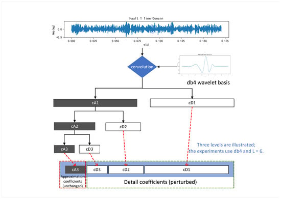
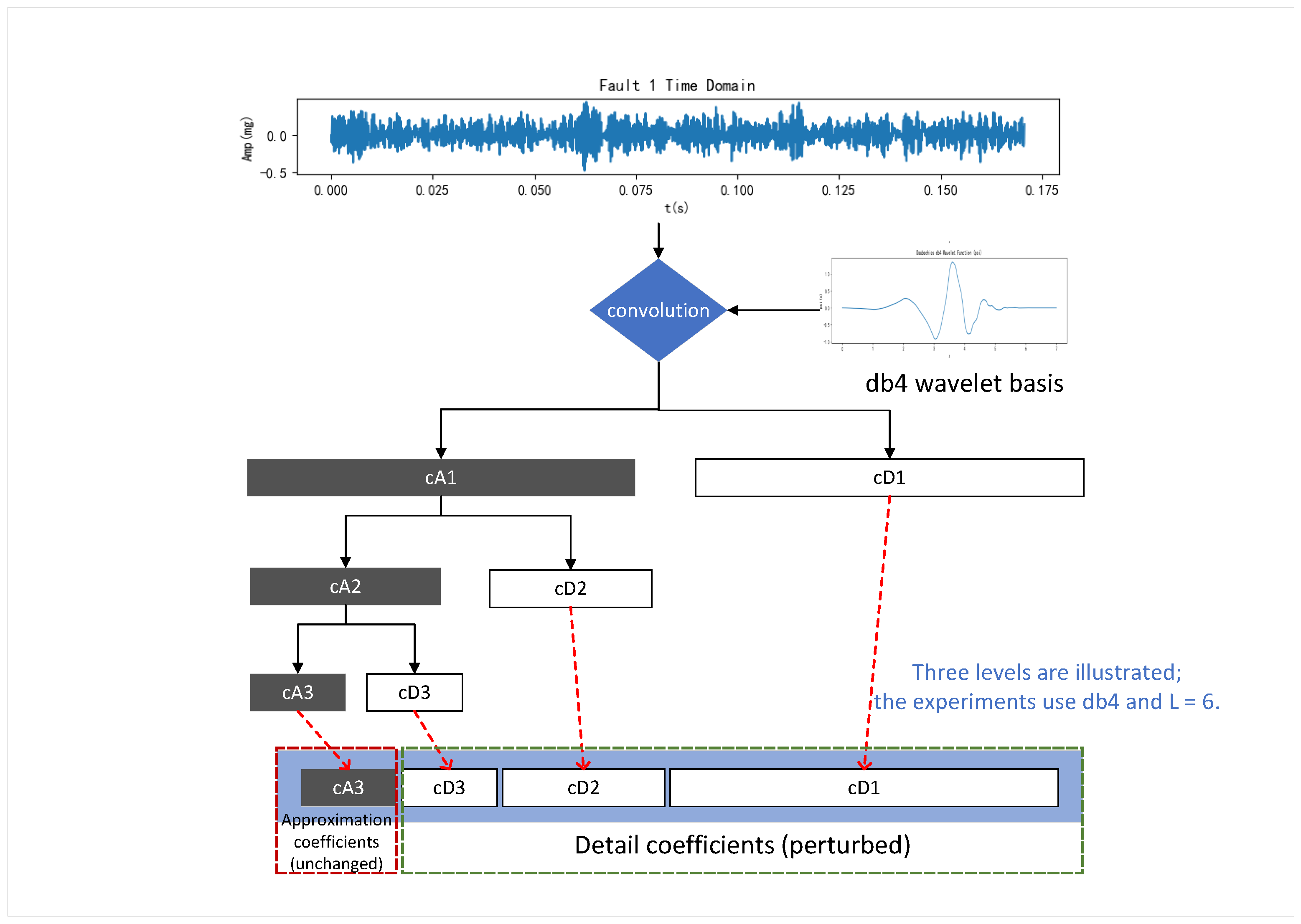
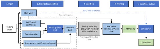
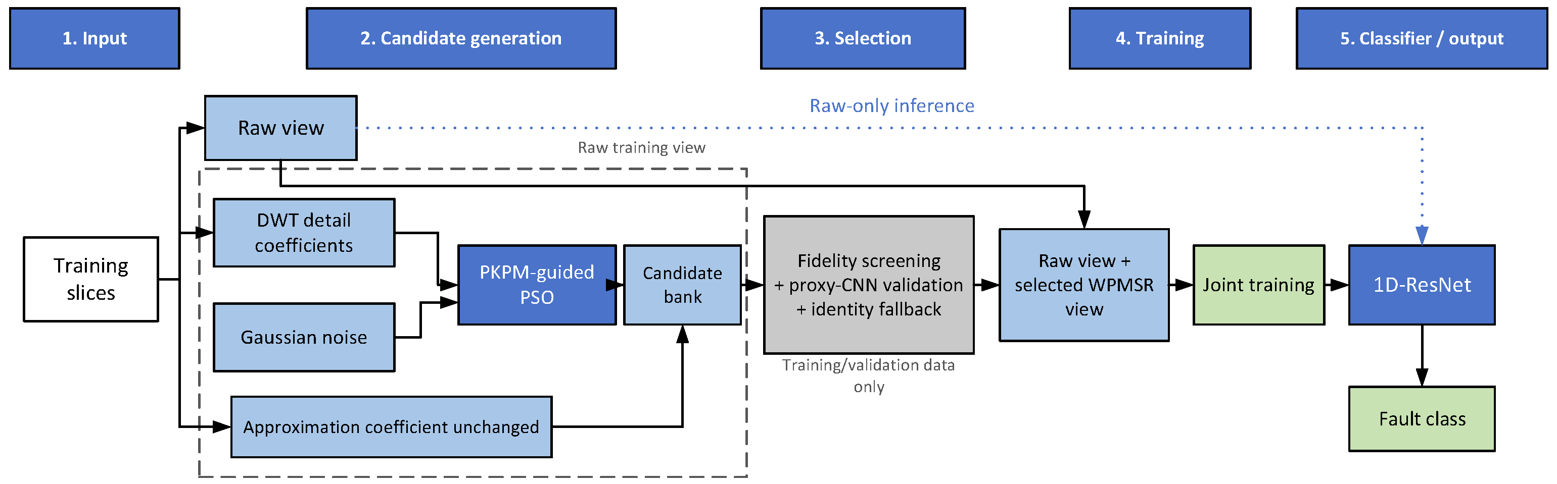
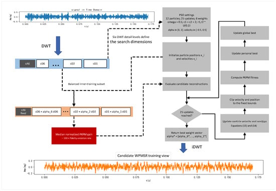
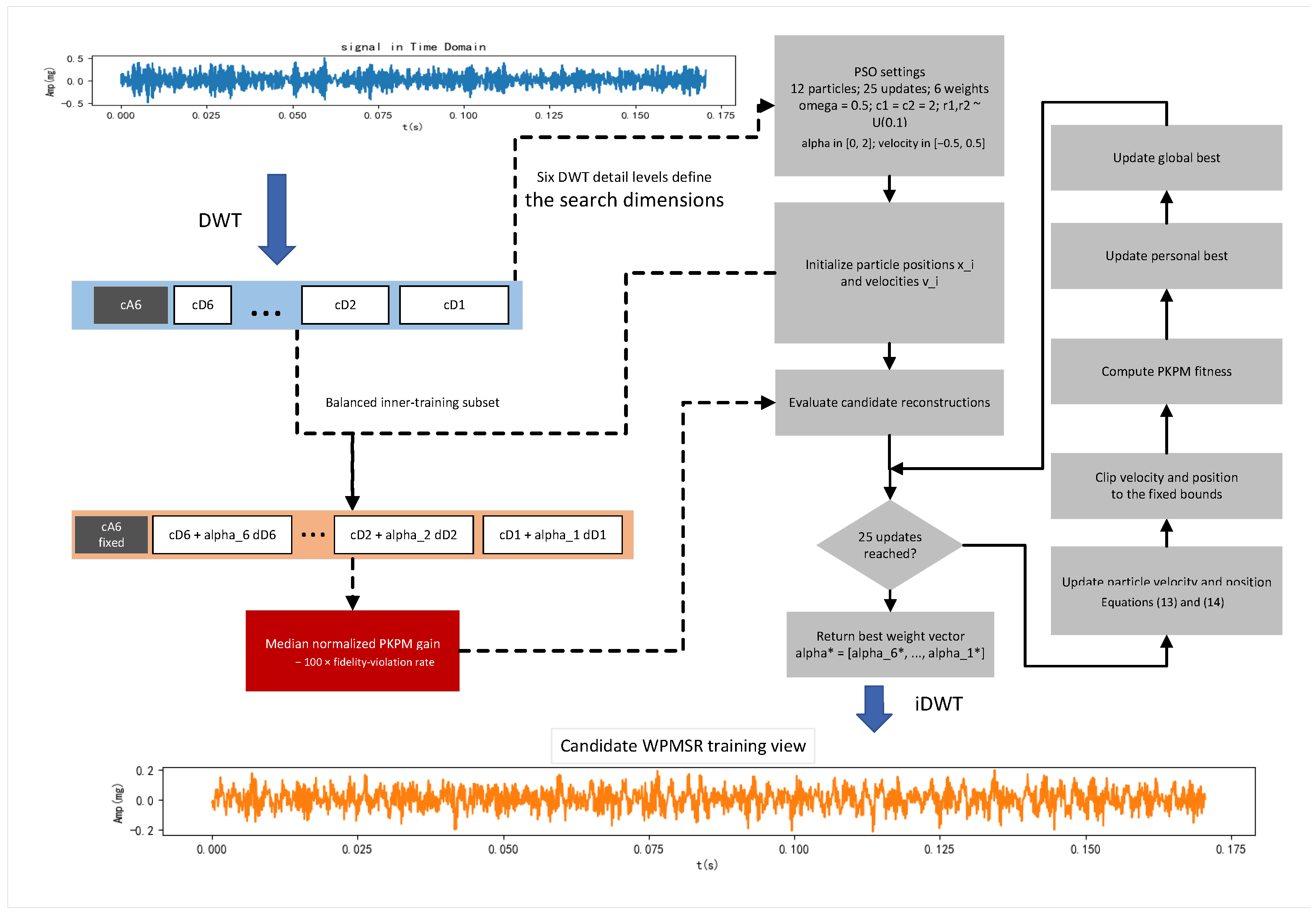
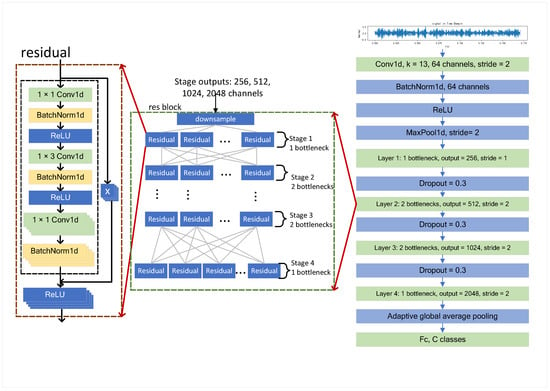
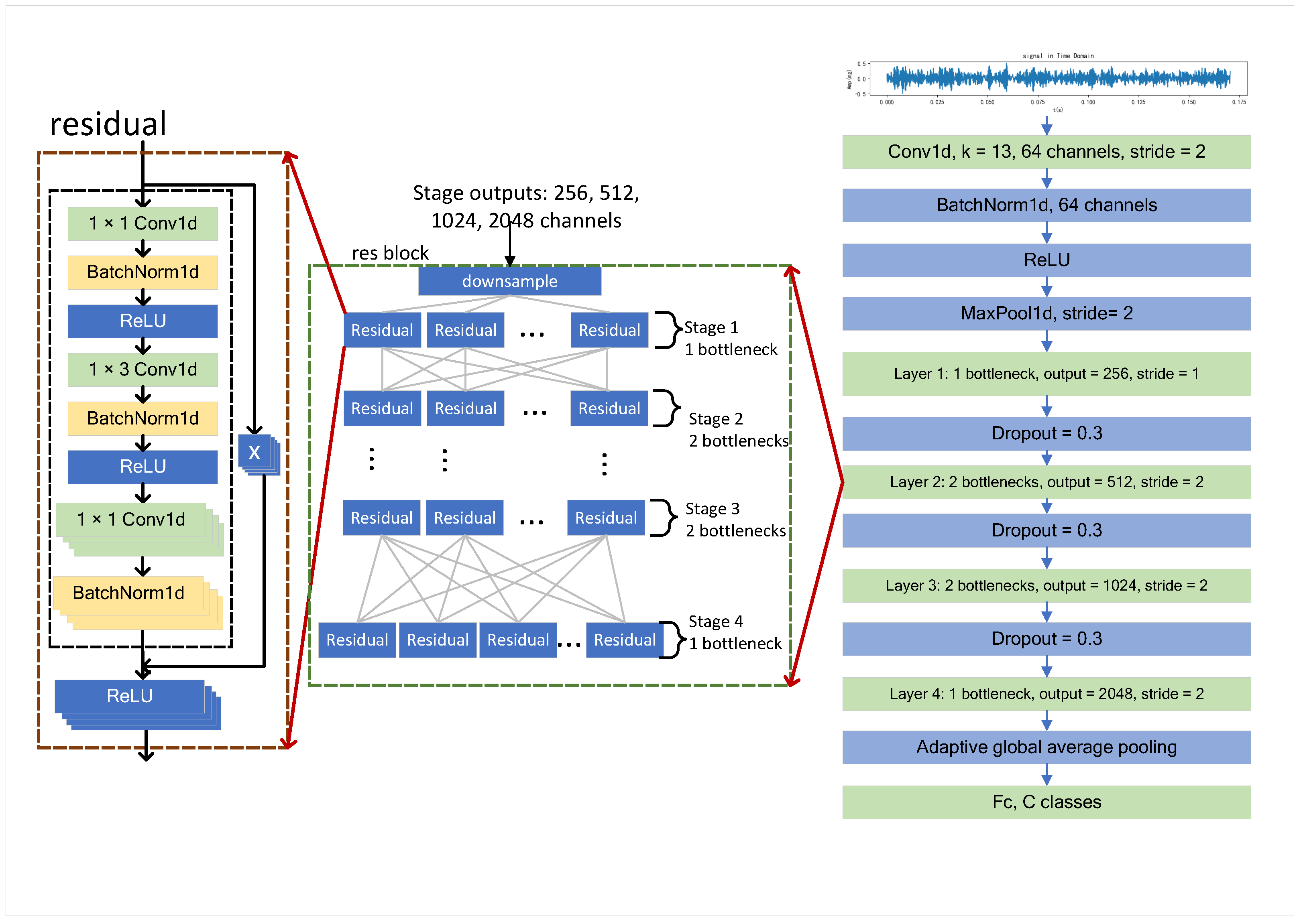
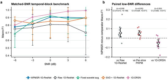
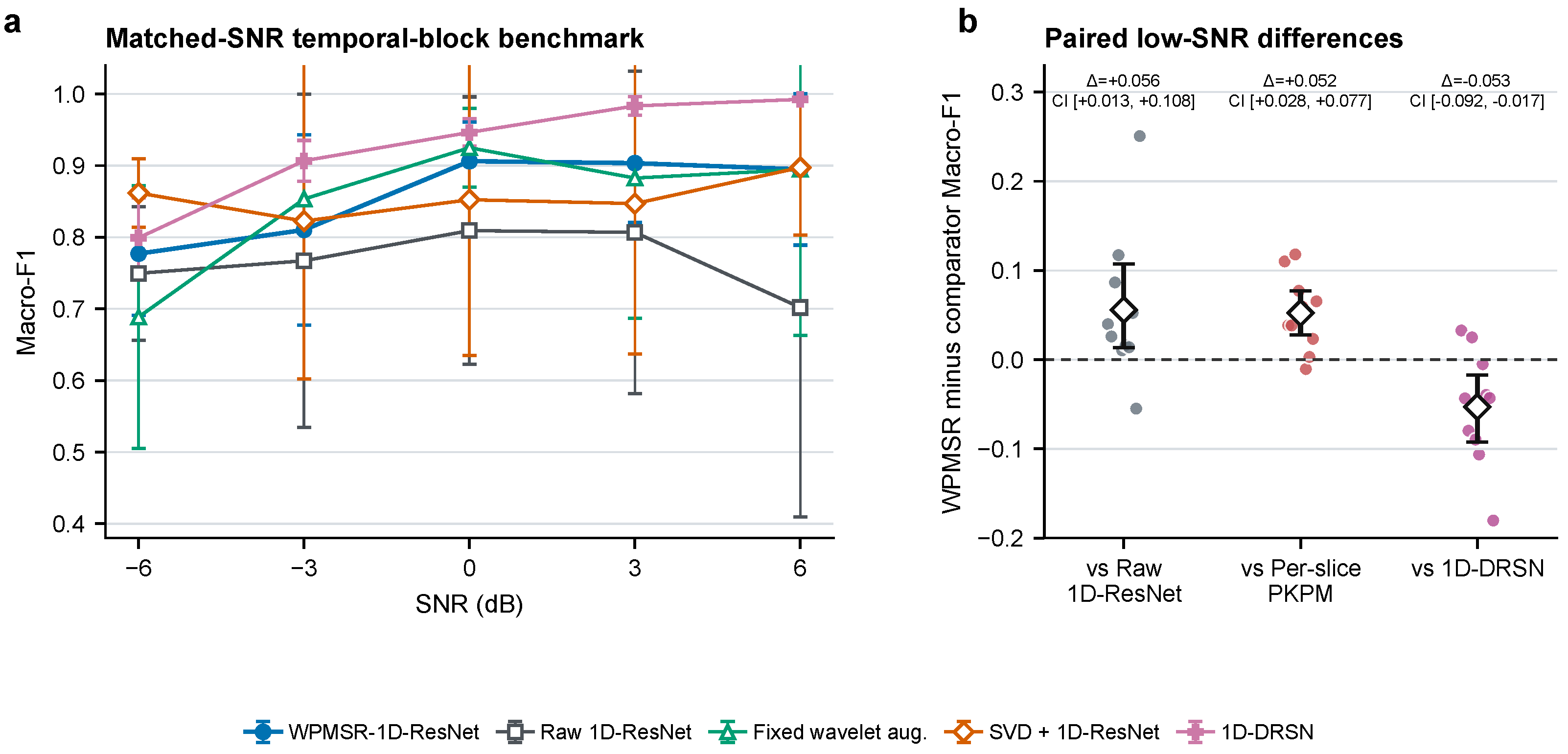
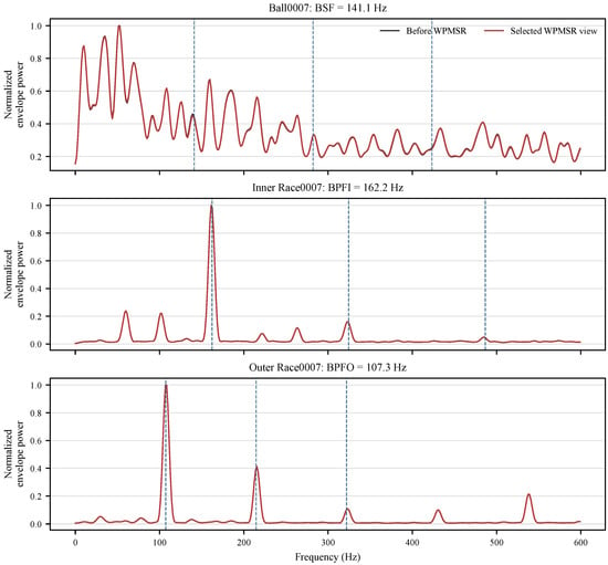
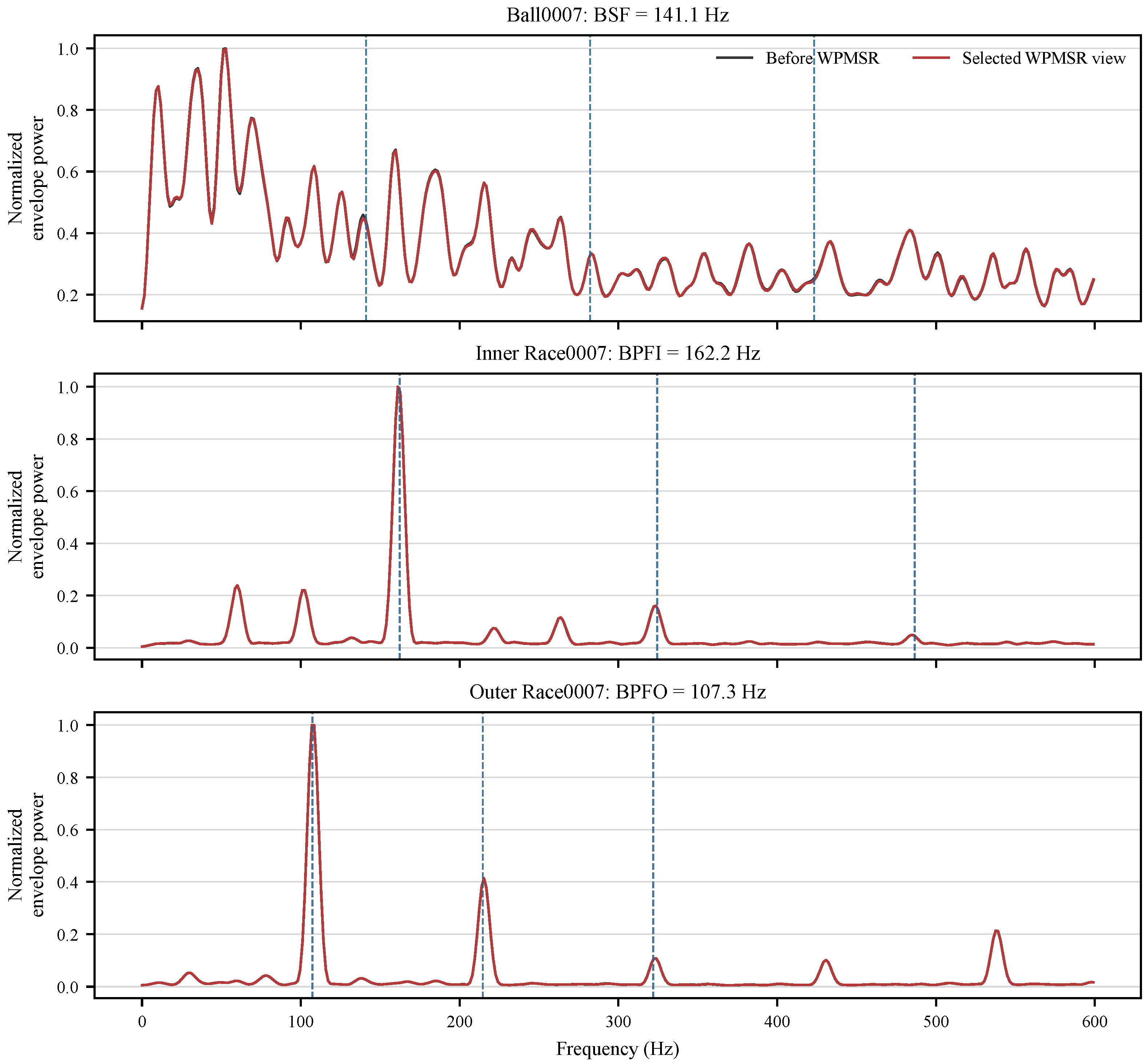
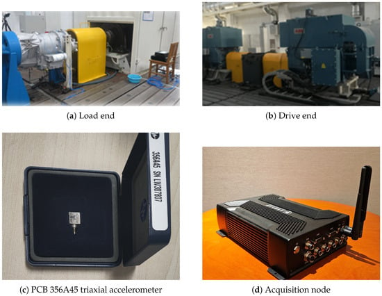
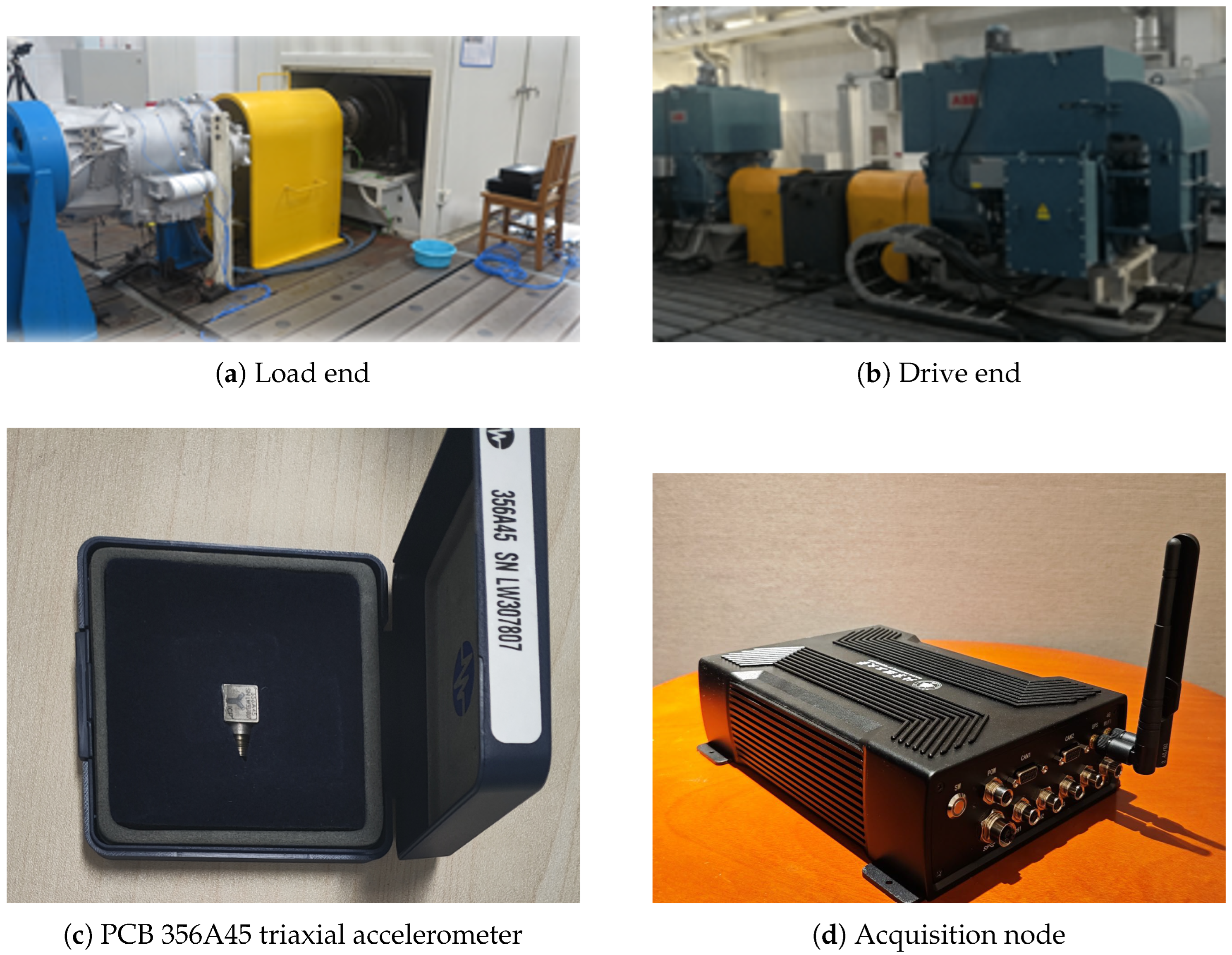

Disclaimer/Publisher’s Note: The statements, opinions and data contained in all publications are solely those of the individual author(s) and contributor(s) and not of MDPI and/or the editor(s). MDPI and/or the editor(s) disclaim responsibility for any injury to people or property resulting from any ideas, methods, instructions or products referred to in the content. |
© 2026 by the authors. Licensee MDPI, Basel, Switzerland. This article is an open access article distributed under the terms and conditions of the Creative Commons Attribution (CC BY) license.