


Abstract
Pressure losses in heating, ventilation, and air-conditioning (HVAC) duct elbows significantly increase fan power requirements and reduce overall system efficiency. This study presents a comprehensive computational fluid dynamics (CFD) investigation aimed at identifying effective strategies for reducing pressure losses in 90° HVAC duct elbows. The numerical methodology was first validated against published experimental measurements, demonstrating excellent agreement and providing confidence in the predictive capability of the CFD model. The validated model was then employed to evaluate the influence of duct geometry, inlet velocity, guide vane configuration, inter-vane spacing, perforated guide vanes, and duct material roughness on aerodynamic performance using the SST k–ω turbulence model. The results show that round elbows reduce pressure losses by approximately 50% compared with hydraulically equivalent rectangular elbows, highlighting the strong influence of duct geometry on flow separation. Among the flow-control strategies investigated, curved guide vanes produced the greatest improvement, with an optimized three-vane arrangement and a non-dimensional spacing of (corresponding to 150 mm for the specific geometry tested) reducing pressure losses by approximately 31% relative to the baseline elbow without guide vanes. In contrast, the investigated perforated guide vane provided only marginal improvement, indicating that its geometry requires further optimization to minimize blockage and mixing losses. The material roughness study showed that smooth, rigid duct materials produced only minor differences in pressure loss, whereas flexible ducts generated noticeably higher losses because of their increased surface roughness. These findings demonstrate that optimizing elbow geometry and guide vane design is considerably more effective than modifying duct material or using the investigated perforated vane configuration. The study provides practical design recommendations for improving the aerodynamic performance and energy efficiency of HVAC duct systems.
1. Introduction
Duct elbows are essential components in heating, ventilation, and air-conditioning (HVAC) systems, enabling airflow direction changes within the spatial constraints of buildings.
However, these fittings introduce significant aerodynamic losses due to abrupt flow direction changes, flow separation, secondary flow formation, and local recirculation [1]. In typical HVAC systems, duct elbows can account for 30–50% of total system pressure losses, directly impacting fan energy consumption and overall system efficiency [2].
The aerodynamic performance of duct elbows depends on multiple parameters, including geometry (aspect ratio, turning angle), flow conditions (Reynolds number, inlet velocity), internal features (guide vanes, turning vanes), and surface characteristics (material roughness) [3]. Among these, the installation of guide vanes represents one of the most effective passive flow control methods for reducing pressure losses in rectangular elbows [4].
Previous experimental and numerical studies have investigated various aspects of duct elbow aerodynamics. Work [3] conducted comprehensive experimental measurements of pressure losses in flat-oval duct elbows, establishing benchmark data for CFD validation. Work [2] developed a CFD-based procedure for predicting pressure loss coefficients of duct fittings, demonstrating the applicability of numerical methods in HVAC design. However, systematic parametric studies investigating the combined effects of guide vane configurations, perforation strategies, and material selection remain limited in the literature.
1.1. Research Gap and Novelty
While previous studies have investigated individual aspects of duct elbow performance, several critical gaps remain:
- Integrated Parametric Study: No single study has systematically investigated the combined effects of duct geometry, guide vane configuration, inter-vane spacing, perforated guide vanes, and material roughness within a unified CFD framework using consistent validation and mesh convergence criteria.
- Perforated Guide Vane Assessment: Limited literature exists on perforated guide vanes for HVAC applications, and the physical mechanisms (pressure equalization, boundary layer re-energization, and wake reduction) have not been systematically analyzed.
- Non-dimensional Design Guidelines: Previous studies have reported dimensional results (e.g., “150 mm spacing”) without providing non-dimensional parameters that allow generalization to different duct sizes.
- Material Roughness Impact: The quantitative effect of different duct materials (UPVC, aluminum, galvanized steel, flexible duct) on pressure losses in elbows has not been systematically compared under identical flow conditions.
1.2. Scientific Contribution
This study provides the following novel contributions:
- Comprehensive Parametric Database: A systematic dataset of pressure loss coefficients for 90° HVAC duct elbows under various geometric and flow conditions, validated against experimental data.
- Non-dimensional Design Guidelines: The first study to provide non-dimensional design guidelines for curved plate guide vanes, including an optimal spacing ratio () that differs significantly from existing ASHRAE recommendations for airfoil-shaped turning vanes.
- Physical Mechanism Analysis: A detailed analysis of secondary flows, vortical structures, and energy dissipation mechanisms in duct elbows with and without flow control devices.
- Perforated Vane Assessment: The first systematic CFD assessment of perforated curved guide vanes in HVAC duct elbows, including quantification of losses due to jetting, shear layer formation, and recirculation.
- Material Selection Guidance: Quantitative comparison of pressure losses for four common HVAC duct materials under identical flow conditions.
The present research addresses these gaps through a comprehensive CFD investigation comprising four interconnected studies:
- Flow Regime Analysis: Investigation of pressure-loss characteristics in rectangular and round 90° duct elbows over a representative turbulent Reynolds number range representative of HVAC operating conditions, with a comparison between the two duct geometries.
- Guide Vane Sensitivity Study: Evaluation of curved guide vane configurations and a parametric investigation of inter-vane spacing to identify the best-performing arrangement for minimizing pressure losses and improving flow uniformity. (Note: While a full optimization is beyond the scope of this work, a systematic sensitivity study was conducted to establish the influence of spacing on performance).
- Perforated Guide Vane Assessment: Investigation of the aerodynamic performance of perforated guide vanes. The concept behind this design is to mitigate the adverse pressure gradient that forms across a solid vane. By allowing a controlled bleed flow through the perforations, the pressure on the high-pressure (pressure) side and the low-pressure (suction) side of the vane can be partially equalized. This pressure equalization is intended to reduce the strength of the secondary flows and the separated region downstream of the vane, thereby reducing the total pressure loss.
- Material Roughness Assessment: Evaluation of the influence of duct wall roughness and commonly used HVAC duct materials on pressure-loss characteristics.
The numerical methodology was first validated against the experimental measurements of [3].
The findings provide practical design guidelines for HVAC engineers regarding duct geometry selection, guide vane implementation, and material selection to improve aerodynamic performance and reduce energy consumption.
1.3. Novelty and Contribution
While individual findings such as “round elbows outperform rectangular elbows” and “guide vanes reduce losses” are well established in the literature, the novelty of this study lies in the following aspects:
- Integrated Parametric Study: No previous study has systematically investigated all of the following parameters within a single, unified CFD framework using consistent validation and mesh convergence criteria:
- Duct geometry (rectangular vs. round);
- Guide vane configuration (0, 1, 2, and 3 vanes);
- Inter-vane spacing (parametric sensitivity study);
- Perforated guide vanes (novel concept assessment);
- Material roughness (four common HVAC materials).
- Non-dimensional Design Guidelines: This study is the first to provide non-dimensional design guidelines for curved plate guide vanes specifically for HVAC duct elbows. The finding that the optimal spacing () is significantly smaller than the ASHRAE recommendation for airfoil-shaped turning vanes (1.5–2.0 × D_h) represents a novel and practically important contribution.
- Perforated Vane Assessment: This study provides the first systematic CFD assessment of perforated curved guide vanes in HVAC duct elbows, including quantification of the losses due to jetting, shear layer formation, and recirculation. The finding that the current perforation design provides only marginal improvement (1.3%) and the identification of the underlying physical mechanisms represent a novel contribution.
- Quantitative Material Comparison: This study provides a quantitative comparison of pressure losses for four common HVAC duct materials (UPVC, aluminum, galvanized steel, and flexible duct) under identical flow conditions. The finding that flexible ducts increase pressure losses by approximately 13% compared to galvanized steel provides a quantitative basis for material selection decisions.
- Comparison with Established Guidelines: This study provides a critical comparison of the findings with established design guidelines (ASHRAE Handbook), highlighting discrepancies and providing refined recommendations based on the specific vane geometry and flow conditions.
2. Literature Review
2.1. Pressure Loss Mechanisms in Duct Elbows
The pressure loss in duct elbows arises from two primary mechanisms: friction losses along the duct walls and dynamic losses due to flow direction changes [5]. As airflow enters a 90° elbow, the centrifugal force causes the flow to migrate toward the outer wall, creating an adverse pressure gradient along the inner wall [6]. This pressure gradient triggers boundary layer separation, forming a recirculation zone near the inner bend [7]. The separated flow region reduces the effective flow area, accelerates the remaining flow, and generates turbulent mixing, all contributing to increased pressure losses [8].
For rectangular elbows, additional losses arise from secondary flows and a non-uniform velocity distribution at the outlet [9]. The aspect ratio significantly influences the loss coefficient, with higher aspect ratios generally producing lower losses due to reduced corner vortices [10]. The total pressure loss coefficient (K) for an elbow is typically expressed as [11]:
where ∆Pt is the total pressure drop, ρ is the air density, and V is the average velocity.
The rationale for using perforated guide vanes is rooted in the concept of pressure equalization. When a solid guide vane is placed in a curved duct, a significant pressure difference develops between the vane’s pressure side (facing the outer wall of the elbow, where the velocity is lower and the pressure is higher) and its suction side (facing the inner wall, where the velocity is higher and the pressure is lower). This pressure differential drives a secondary flow around the trailing edge of the vane, contributing to wake formation and mixing losses [12,13,14,15,16,17,18,19].
Introducing perforations into the vane surface creates a pathway for a small, controlled amount of bleed flow from the high-pressure side to the low-pressure side. This bleed flow is hypothesized to perform two beneficial functions [20,21]:
Boundary Layer Re-energization: The bleed flow can re-energize the boundary layer on the suction side of the vane, delaying or suppressing flow separation. This reduces the size of the wake and the associated momentum deficit downstream.
Pressure Gradient Reduction: By equalizing the pressure on both sides of the vane, the perforations reduce the driving force for the secondary flow around the vane’s trailing edge. This leads to a more uniform velocity profile at the elbow outlet and a reduction in turbulent mixing losses [22,23].
However, the net effect is highly sensitive to the design of the perforations. If the hole size or open area ratio is not optimized, the bleed flow itself can become a source of losses, introducing jetting, edge effects, and additional turbulence generation [23].
2.2. Guide Vanes and Flow Control
Guide vanes (also called turning vanes) represent the most common passive flow control method for reducing pressure losses in rectangular duct elbows [12]. Their primary function is to divide the main flow into smaller passages, reducing the severity of flow turning and limiting separation [13]. Guide vanes can be classified as flat, curved, or airfoil-shaped, with curved vanes generally providing superior performance [14].
The number of guide vanes significantly influences performance. While additional vanes improve flow guidance, they also increase the wetted surface area and friction losses [15]. The optimal number of vanes represents a balance between these competing effects. Previous studies have identified that 2–4 vanes typically provide the best performance for rectangular elbows [16].
Inter-vane spacing is another critical parameter. Unequal spacing can lead to a non-uniform velocity distribution and increased losses [17]. The ASHRAE Handbook [18] recommends spacing turning vanes at approximately 1.5–2 times the duct hydraulic diameter for airfoil-shaped turning vanes, which are designed to minimize flow blockage while providing smooth flow guidance. However, this recommendation is specific to airfoil-type turning vanes and may not be directly applicable to simpler curved plate guide vanes, where the optimal spacing is expected to be smaller due to differences in the vane’s aerodynamic profile and blockage characteristics. The optimal spacing ultimately depends on the specific vane geometry, duct aspect ratio, and flow conditions, highlighting the need for case-specific investigations.
2.3. Perforated Guide Vanes
Perforated guide vanes represent an emerging concept where openings are introduced into the vane surface to allow pressure equalization between the vane’s pressure side (facing the outer wall of the elbow, where the flow decelerates and the static pressure is higher) and its suction side (facing the inner wall, where the flow accelerates and the static pressure is lower). This pressure differential is a primary driver of secondary flows and wake formation downstream of the vane [19,20,21].
The concept is analogous to flow conditioning using perforated plates, where controlled bleeding through openings has been shown to reduce pressure imbalances and improve downstream flow uniformity [22]. However, the introduction of perforations also creates new sources of losses. Each opening acts as an abrupt edge, generating local flow acceleration, jetting effects, and additional turbulence generation immediately surrounding the perforation boundaries [23]. Furthermore, the solid material remaining between the holes still contributes to flow blockage, and if the open area ratio is too high, the structural integrity of the vane may be compromised [24].
The net effect of a perforated guide vane is therefore highly sensitive to the design parameters, including:
Perforation diameter and open area ratio: Larger holes and higher open area ratios allow more bleed flow but also create larger edge effects and local losses.
Hole distribution pattern: The location of the holes along the vane surface determines where the bleed flow is introduced and how effectively it re-energizes the boundary layer on the suction side [25].
Previous Investigations
Limited literature exists on perforated guide vanes specifically, with most studies focusing on solid turning vanes or airfoil-shaped vanes [26]. However, several related investigations provide context for the present study.
Study [19] conducted an experimental study on perforated turning vanes in a 90° rectangular duct elbow. They tested vanes with various open area ratios (ranging from 10% to 30%) and found that a moderate open area ratio of approximately 20% provided the lowest pressure loss, with a reduction of approximately 8% compared to a solid vane. However, they observed that higher open area ratios (>25%) actually increased losses due to excessive jetting and mixing at the perforation edges.
Work [22] performed a numerical investigation of perforated plates used as flow conditioners upstream of duct elbows. They found that the effectiveness of the perforations was highly dependent on the hole distribution pattern. Perforations concentrated near the center of the plate were more effective at reducing the pressure imbalance than uniformly distributed holes, as the center region experiences the highest pressure differential.
Study [23] provided a comprehensive review of guide vane technologies for HVAC duct systems. They noted that while the concept of perforated vanes is promising, most studies have focused on solid vanes, and the limited data on perforated vanes show mixed results. They concluded that the performance of perforated vanes is highly case-specific and that systematic parametric studies are needed to identify optimal perforation designs for different duct geometries and flow conditions.
In the present study, perforated guide vanes achieved only a modest reduction in pressure loss (approximately 2–3%) compared with conventional solid guide vanes. This limited improvement is attributed to the additional viscous friction introduced by the perforations, which offsets the benefit of pressure equalization.
These previous studies indicate that the concept of perforated guide vanes is viable but requires careful optimization of the perforation parameters. The mixed results reported in the literature highlight the need for case-specific investigations, which is the motivation for the present study. The present investigation builds on this prior work by examining a specific perforation configuration (180 mm holes, 22.7% open area ratio) in a rectangular duct elbow, with the aim of assessing whether the performance benefits observed in some studies can be replicated in this geometry.
2.4. Effect of Duct Material Roughness
Internal wall roughness affects the friction factor in duct systems, with rougher surfaces producing higher pressure losses [24]. Common HVAC duct materials exhibit different surface roughness characteristics, which influence wall friction and, consequently, the total pressure loss within duct systems. Typical absolute roughness values include galvanized steel (0.00015 m), aluminum (0.00009 m), UPVC (0.00001 m), and flexible duct materials (0.0005–0.001 m) [25]. Although pressure losses in duct elbows are primarily governed by flow separation and secondary flow structures, wall roughness contributes to the overall pressure loss and may become increasingly important when comparing materials under identical elbow geometries and operating conditions. Therefore, evaluating the influence of duct material roughness is relevant for improving the aerodynamic performance and energy efficiency of HVAC duct systems.
CFD Methodology in Duct Flow Analysis
Computational Fluid Dynamics has become the standard tool for HVAC duct design and analysis [27]. The Reynolds-Averaged Navier–Stokes (RANS) approach, coupled with appropriate turbulence models, provides accurate pressure loss predictions at an acceptable computational cost [28]. The SST k-ω model is particularly well suited for duct elbow analysis due to its improved near-wall prediction and response to adverse pressure gradients [29,30,31,32,33,34].
The numerical methodology adopted in the present study was validated against the experimental measurements [3], as documented in the ASHRAE Research Project RP-1493 framework [35,36,37,38,39,40]. This framework provides standardized geometry (a 90° flat-oval duct elbow), boundary conditions (a velocity range of 12–30 m/s, corresponding to dynamic pressures of 100–500 Pa), and performance metrics (total pressure drop between upstream and downstream measurement planes) specifically for validating CFD predictions of duct fitting pressure losses.
For the validation exercise, we reproduced the experimental geometry and boundary conditions using the SST k–ω turbulence model. Pressure drop predictions were compared with the experimental data at five dynamic pressure levels (100, 200, 300, 400, and 500 Pa). The validation results, presented in Section 4.1, demonstrate excellent agreement with the experimental data (R2 ≈ 0.99), confirming that the CFD model accurately captures the pressure loss behavior of the duct elbow and is suitable for the parametric investigations conducted in this study.
3. Methodology
3.1. Overview of CFD Approach
The numerical investigations were performed using ANSYS Fluent 2025 R2 (AN-SYS, Inc., Canonsburg, PA, USA). A pressure-based, steady-state solver was employed with the SIMPLE algorithm for pressure–velocity coupling. Second-order upwind discretization was used for the momentum and turbulence transport equations to minimize numerical diffusion. The SST k-ω turbulence model was selected for all production runs due to its demonstrated accuracy in separated and adverse pressure gradient flows [36].
Turbulence Model Selection for Validation
To establish confidence in the numerical methodology, the validation study (Section 3.2) was conducted using three different turbulence models: the SST k–ω (which is also used for all production runs), the standard k–ε, and the Reynolds Stress Model (RSM). The latter two models were included specifically to enable direct comparison with the original benchmark study [3], which employed these models in their CFD analysis. This approach allows us to assess the sensitivity of the pressure loss predictions to the choice of turbulence model and to benchmark our results against commonly reported literature values. The validation results, presented in Section 4.1, show that all three models produced similar results, with the SST k–ω model providing slightly better agreement with the experimental data at higher dynamic pressures. The governing equations solved were the Reynolds-Averaged Navier–Stokes (RANS) equations:
Continuity equation (incompressible flow):
Reynolds-Averaged Navier–Stokes (RANS) momentum equation:
where
- = mean velocity component in direction ;
- = mean pressure;
- = fluid density;
- = dynamic viscosity;
- = Reynolds stress tensor (from turbulence).
The Reynolds stresses were modeled using the SST k-ω turbulence model, which combines the standard k-ω model in the near-wall region with the k-ε model in the free stream [37].
3.2. Validation Study
3.2.1. Geometry and Computational Domain
The validation study reproduced the experimental work [3], as documented in the ASHRAE Research Project RP-1493 framework [35]. The geometry consisted of a 90° flat-oval duct elbow without turning vanes, with the following cross-sectional dimensions:
- Major axis (A): 356 mm;
- Minor axis (a): 152 mm.
The flat-oval cross-section (Figure 1) was selected to match the experimental setup.
Figure 1.
Flat-oval duct geometry and elbow configuration used in the validation case. The figure shows the flat-oval cross-section and elbow configuration with the specified dimensions.
Upstream and downstream duct lengths were based on ASHRAE Standard 120 [38]:
- Upstream length: 11.5Dh;
- Downstream length: 15Dh.
where Dh is the hydraulic diameter calculated as:
The computational domain included extended straight sections upstream and downstream of the elbow to ensure fully developed flow at the measurement planes.
Measurement planes were defined in regions of fully developed flow, with PL-1 equivalent upstream and PL-2 equivalent downstream, following the experimental methodology. The “up” plane (PL-1) was located 11.5Dh upstream of the elbow inlet, and the “down” plane (PL-2) was located 15Dh downstream of the elbow outlet, ensuring measurements in fully developed flow regions as per ASHRAE Standard 120 [38].
3.2.2. Boundary Conditions
Table 1 presents the boundary conditions applied in the validation study. The velocity range was selected to match the dynamic pressure range (100–500 Pa) from the validation dataset, ensuring consistency with the experimental conditions.
Table 1.
Summary of numerical setup and boundary conditions used in the validation study.
As the production CFD model adopts the SST k–ω turbulence model, the validation study was primarily conducted using the same model to ensure direct applicability. The standard k–ε and the RSM are included additionally to assess model sensitivity and to benchmark against commonly reported literature values.
3.2.3. Numerical Setup
The numerical setup for the validation study was as follows:
- Solver type: Pressure-based;
- Flow regime: Steady-state;
- Turbulence models:
- ○
- Primary: SST k–ω (matching the production model);
- ○
- Secondary (for sensitivity comparison): Standard k–ε and Reynolds Stress Model (RSM).
- Spatial discretization:
- ○
- Momentum: QUICK scheme;
- ○
- Pressure: Standard scheme.
- Convergence criterion: Residuals < for all conserved variables.
This setup ensures that the validation results are directly relevant to the production simulations, while the additional turbulence models provide context for understanding model-induced uncertainties.
3.2.4. Mesh Independence Study
A systematic mesh independence study was performed for the validation case following the Grid Convergence Index (GCI) methodology [30,31,32,33]. Three meshes with systematically refined cell counts were generated. The pressure drop at a dynamic pressure of 300 Pa was used as the comparison metric.
Table 2 presents the results of the mesh independence study. The medium mesh (0.61M cells) was selected for the production runs, as the GCI value of 2.8% indicated acceptable numerical uncertainty, and further refinement to the fine mesh provided negligible improvement (0.91% change in pressure drop). The mesh refinement ratio was approximately 2, consistent with recommended practices.
Table 2.
Mesh Independence Test Results for the Validation Case.
3.3. Velocity Effects Study
Geometry and Boundary Conditions
Two duct elbow geometries were investigated to assess the influence of velocity on flow development and pressure losses:
- Rectangular elbow—A 90° elbow with a rectangular cross-section having an aspect ratio of 2:1 (width:height). The duct dimensions were selected to match standard HVAC system practice, with a hydraulic diameter of approximately 0.3 m and a centerline bend radius-to-diameter ratio of 1.5. The upstream and downstream straight duct lengths were each set to 10 hydraulic diameters to ensure fully developed inlet flow and recovery at the outlet.
- Round elbow—A 90° smooth-bend circular elbow with a diameter equal to the hydraulic diameter of the rectangular case (0.3 m), maintaining the same centerline bend radius-to-diameter ratio (1.5) for direct comparability. This geometry serves as a baseline to isolate the effect of cross-sectional shape.
Both geometries were modeled as 3D steady-state domains using the same numerical framework. Table 3 shows boundary conditions applied in the velocity effects study. Appendix A shows CFD Setting s Details.
Table 3.
Boundary conditions applied in the velocity effects study.
The velocity ranges were chosen to cover typical HVAC operating conditions while ensuring that the round-elbow cases (10–12 m/s) overlap with the rectangular-elbow dataset for direct shape comparison at equivalent dynamic pressures.
3.4. Guide Vane Optimization Study
Four elbow configurations were investigated.
Table 4 presents the four guide vane configurations investigated. The duct cross-sectional dimensions and flow boundary conditions were kept constant in all cases to isolate the effect of the guide vane arrangement.
Table 4.
Guide Vane Configuration Cases.
The three-vane configuration was further optimized by varying the inter-vane spacing:
Table 5 presents the inter-vane spacing cases investigated. The middle guide vane was fixed as a reference, and the adjacent vanes were repositioned to achieve the desired spacing. This approach ensured that the effect of spacing could be isolated while keeping the main vane location consistent between cases.
Table 5.
Inter-Vane Spacing Cases.
The duct and boundary conditions for the guide vane study were:
- Duct cross-sectional dimensions: 750 mm × 1500 mm (aspect ratio 2:1);
- Elbow angle: 90°;
- Working fluid: Air at 15 °C (288.15 K);
- Air density: 1.225 kg/m3;
- Dynamic viscosity: 1.7894 × 10⁻⁵ kg/m·s;
- Inlet velocity: 8.0 m/s (all cases);
- Outlet gauge pressure: 0 Pa;
- Wall condition: No-slip wall;
- Inlet turbulence intensity: 5%;
- Inlet turbulent viscosity ratio: 10.
The duct cross-sectional area was:
The corresponding airflow rate was:
where:
- (shorter side);
- (longer side).
This confirmed a fully turbulent internal duct-flow condition ().
The dynamic pressure was:
Figure 2 shows cross-sectional schematic of the square duct equipped with three curved turning vanes at a uniform inter-vane spacing.
Figure 2.
Cross-sectional schematic of the 90° square duct elbow (750 mm × 750 mm) equipped with three curved turning vanes at a uniform inter-vane spacing of s = 150 mm (s/Dh = 0.20).
Additional Mesh Independence for Guide Vane Cases
A separate mesh independence study was conducted for the three-vane configuration with 150 mm spacing. Three mesh densities were tested, using the total pressure drop as the metric for comparison.
Table 6 presents the mesh independence results for the guide vane case. The medium mesh (1.2M cells) was selected for the production runs, with a GCI of 1.8%, indicating acceptable numerical uncertainty for the small pressure differences between configurations.
Table 6.
Mesh Independence Test for Guide Vane Configuration (Three Vanes, 150 mm Spacing).
3.5. Perforated Guide Vane Study
A perforated curved guide vane was designed with a projected circular hole pattern.
Table 7 presents the specifications of the perforated guide vane. The holes were projected onto the curved vane surface in SpaceClaim (ANSYS, Inc.), resulting in elliptical openings due to surface curvature.
Table 7.
Perforated Guide Vane Specifications.
Figure 3 shows the perforation layout on the guide vane surface, with the 5 × 3 hole pattern and spacing dimensions indicated.
Figure 3.
Perforation layout used for the guide vane surface. The figure shows the 5 × 3 hole pattern with 300 mm horizontal and 373 mm vertical spacing.
Figure 4 shows the 3D geometry of the perforated curved guide vane after projection, with the elliptical openings clearly visible.
Figure 4.
Perforated curved guide vane geometry after projecting the circular holes onto the curved surface. The projection resulted in elliptical openings on the curved vane surface.
The mesh for the perforated vane case consisted of:
- Mesh type: Polyhedral volume mesh;
- Total cells: ≈821,632 cells;
- Minimum orthogonal quality: ≈0.20.
The mesh for the perforated vane configuration was generated using a polyhedral volume mesh with a minimum orthogonal quality of approximately 0.20.
Table 8 presents the boundary conditions applied in the perforated vane study.
Table 8.
Boundary Conditions for Perforated Vane Study.
3.6. Material Roughness Study
Four duct materials with different roughness heights were investigated:
Table 9 presents the four material cases investigated. Only the wall roughness changed between cases, whereas the geometry, mesh, turbulence model, and velocity conditions remained constant.
Table 9.
Material Roughness Cases.
The boundary conditions for the material roughness study were:
- Inlet velocity: 8 m/s;
- Outlet: Pressure outlet (0 Pa);
- Fluid: Air;
- Model: SST k-ω;
- Roughness constant: 0.5;
- Gravity: Off.
3.7. Uncertainty Quantification Framework
To ensure the reliability of the numerical results, the following uncertainty quantification framework was adopted:
3.7.1. Discretization Error
The discretization error was quantified using the Grid Convergence Index (GCI) method of Roache [30]. For each configuration, the GCI was calculated using a safety factor of for three-mesh studies. The GCI values for all configurations are summarized in Table 6.
3.7.2. Solution Uncertainty
Solution uncertainty was assessed through:
- Residual Monitoring: All simulations were converged to residuals below for all conserved variables.
- Mass Balance Monitoring: The mass imbalance at the outlet was maintained below 0.1% of the inlet mass flow rate.
- Iteration Independence: For each simulation, the solution was considered converged when the pressure drop changed by less than 0.01% over 100 iterations.
3.7.3. Turbulence Model Sensitivity
The sensitivity to turbulence modeling was assessed in the validation study (Section 3.2) by comparing three turbulence models (SST k–ω, standard k–ε, and RSM). The results showed that all three models produced excellent agreement with the experimental data (R2 ≈ 0.99), with the SST k–ω model providing a balance between accuracy (within ±2% of experimental data) and computational efficiency (approximately 2.5× faster than the RSM).
3.7.4. Combined Uncertainty
The combined numerical uncertainty for each configuration is estimated as:
where is the discretization error, is the turbulence model uncertainty (estimated as ±2% from the validation study), and is the iteration error (negligible for converged solutions). The total uncertainty ranges from 2.5% to 3.5% across the configurations.
4. Results and Discussion
4.1. Validation Results
The CFD-predicted pressure loss was plotted against the dynamic pressure and compared with the experimental data [3].
Figure 5 presents the validation results comparing the CFD predictions with the experimental data. The relationship between the total pressure loss and the dynamic pressure was found to be linear, confirming theoretical expectations. CFD predictions closely matched experimental data, with minor deviations at lower dynamic pressures attributed to numerical diffusion and turbulence modeling limitations.
Figure 5.
Validation of CFD -predicted pressure loss against experimental data [3].
Figure 5 presents the quantitative comparison between the experimental and CFD pressure loss data. The excellent agreement (R2 ≈ 0.99) between the CFD predictions and the experimental data demonstrated that the numerical model accurately captures the pressure loss behavior of the duct elbow. The clear linear relationship confirmed the theoretical proportionality ∆Pt ∝ V2, where the slope represents the loss coefficient of the fitting [39,40,41,42,43]. Table 10 validation Study Pressure Loss Data.
Table 10.
Validation Study Pressure Loss Data.
4.1.1. Model Sensitivity Analysis
The three turbulence models tested in the validation study (SST k–ω, standard k–ε, and RSM) all produced excellent agreement with the experimental data [3], with coefficients of determination of R2 ≈ 0.99 for all models. However, some differences were observed across the dynamic pressure range (100–500 Pa):
Standard k–ε model: This model slightly overpredicted the pressure loss at lower dynamic pressures (100–200 Pa), with a maximum deviation of approximately 3.5% at 100 Pa. At higher dynamic pressures (400–500 Pa), the predictions were within 1.5% of the experimental data.
RSM: The RSM showed the best overall agreement across the entire dynamic pressure range, with deviations within ±1.2% of the experimental data at all five pressure levels. The slightly better performance at higher dynamic pressures (400–500 Pa) is attributed to the model’s ability to capture anisotropic turbulence effects, which become more pronounced at higher Reynolds numbers.
SST k–ω model: The SST k–ω model performed consistently well across the entire dynamic pressure range, with deviations within ±2.0% of the experimental data. While the RSM showed marginally better agreement at higher dynamic pressures, the difference was small (approximately 0.5–1.0% difference in pressure loss predictions) [44,45,46,47,48,49].
4.1.2. Selection of SST k–ω for Production Runs
Despite the RSM showing slightly better agreement with the experimental data, the SST k–ω model was selected for all production runs for the following reasons:
Demonstrated accuracy in separated flows: The SST k–ω model is specifically designed to handle adverse pressure gradients and flow separation, which are the dominant loss mechanisms in duct elbows [36]. While the validation case (flat-oval elbow without vanes) did not exhibit strong separation, the production cases (rectangular elbows with and without guide vanes) involve more complex separation and recirculation zones.
Computational efficiency: The RSM requires solving seven additional transport equations (for the Reynolds stresses), resulting in a significantly higher computational cost (approximately 2–3 times longer simulation time) compared with the SST k–ω model. Given the large number of parametric cases investigated in this study, the computational savings were substantial [50,51,52,53,54,55,56,57,58].
Numerical robustness: The SST k–ω model demonstrated better numerical stability and convergence behavior compared with the RSM, particularly for the more complex geometries involving guide vanes and perforations.
Industry acceptance: The SST k–ω model is widely used and accepted in HVAC duct flow simulations [27,28,29], providing a balance between accuracy and computational cost that is well suited for engineering design studies.
The validation results confirm that the SST k–ω model provides sufficiently accurate predictions (within the ±2% of the experimental data) while offering significant advantages in terms of computational efficiency and robustness. Therefore, it was selected as the primary turbulence model for the parametric investigations presented in Section 4.2, Section 4.3, Section 4.4, Section 4.5, Section 4.6 and Section 4.7.
4.2. Velocity Effects on the Rectangular Elbow
The rectangular elbow with a 2:1 aspect ratio was tested at inlet velocities of 6, 8, 10, and 12 m/s.
Table 11 and Figure 6 present the pressure drop results for the rectangular elbow at different velocities. The results clearly demonstrate that pressure drop increases quadratically with velocity. At 8 m/s, pressure loss increased by 75.94% compared to the 6 m/s baseline (from 14.11 Pa to 24.83 Pa). At 10 m/s, the increase reached 172.89% (38.51 Pa), and at 12 m/s, the pressure loss was approximately 290.50% higher than that at 6 m/s (55.11 Pa) [50,51,52,53,54,55,56,57,58].
Table 11.
Rectangular Elbow Pressure Drop vs. Velocity.
Figure 6.
Pressure drop vs. velocity for rectangular 2:1 elbow. The figure shows the non-linear increase in pressure drop with velocity, following the ∆P ∝ V2 relationship.
This trend follows the principles of fluid mechanics, as pressure losses are proportional to the square of the velocity (∆P ∝ V2). Increasing velocity increases the dynamic pressure, turbulence intensity, and flow separation around elbows. The experimental validation (Section 4.1) confirmed this relationship.
Pressure contours showed stronger pressure gradients at higher velocities, especially near the inner corner of the elbow, where separation occurs.
Table 12 presents the loss coefficient analysis for the rectangular elbow cases. The loss coefficient remained approximately constant (K ≈ 0.63), confirming the proportionality.
Table 12.
Rectangular Elbow Loss Coefficient.
∆Pt ∝ V2. The slight decrease in K with increasing velocity (from 0.640 to 0.625) may be partially attributed to numerical uncertainty at higher velocities, though it is also consistent with the expected marginal reduction in relative losses at higher Reynolds numbers [2].
4.3. Round vs. Rectangular Elbow Comparison
Round elbows were simulated at 10 m/s and 12 m/s and compared with equivalent rectangular elbows.
Table 13 and Figure 7 present the comparison between the round and rectangular elbows. The round elbow demonstrated significantly better aerodynamic performance at both velocities. At 10 m/s, the round elbow reduced the pressure loss by 49.78% compared with the rectangular elbow. At 12 m/s, the reduction reached 50.52%.
Table 13.
Round vs. Rectangular Elbow Pressure Drop.
Figure 7.
Round elbow pressure drop comparison at 10 m/s and 12 m/s. The figure shows that round elbows consistently achieve approximately 50% lower pressure losses at both velocities.
4.4. Flow Field Analysis
4.4.1. Baseline Performance
The baseline elbow without guide vanes showed the highest total pressure drop among all tested configurations.
Table 14 and Figure 8 present the guide vane configuration results. The baseline recorded a total pressure drop of 12.644 Pa. Adding one-guide vane decreased the total pressure drop to 8.8057 Pa, corresponding to a reduction of 30.36%. Adding a second guide vane produced a further reduction to 8.7256 Pa, the lowest value among the studied cases, corresponding to a 30.99% reduction. The three-vane configuration produced a total pressure drop of 8.7732 Pa (30.61% reduction), slightly higher than the two-vane result.
Table 14.
Guide Vane Configuration Results.
Figure 8.
Comparison of the total pressure drop for the tested guide vane arrangements. The figure shows the significant reduction achieved with one-guide vane and the marginal improvements with additional vanes.
4.4.2. Discussion of Vane Performance
Baseline Case (No Vanes)
This behavior is physically expected because the airflow is forced to change direction sharply through the 90° bend. As the flow enters the elbow, the sudden turning generates an adverse pressure gradient, especially along the inner bend. This causes the main stream to move toward the outer wall, while a separated and recirculating region develops near the inner side of the elbow. This separated region reduces the effective flow area and increases local turbulence production, resulting in a non-uniform downstream velocity and a loss of mechanical energy.
One-Guide Vane
The improvement occurs because the guide vane divides the main flow path and helps the air turn more gradually through the bend. Instead of allowing the entire flow to negotiate the elbow as one distorted stream, the vane creates smaller guided passages and reduces the size of the separated region. The one-vane configuration produces a more organized velocity distribution compared with the baseline case. The flow remains better attached along the curvature, and pressure recovery downstream improves.
Two- and Three-Guide Vanes
The two-vane configuration produces the lowest total pressure drop among all cases, achieving a 30.99% reduction relative to the baseline. The three-vane configuration yields a slightly higher total pressure drop of 8.7732 Pa (30.61% reduction), marginally exceeding the two-vane result. It is very likely that the results with one-, two-, or three-guide vanes lie within the numerical uncertainty, as the authors themselves raise this potential issue later in the discussion.
4.5. Inter-Vane Spacing Sensitivity
The three-guide vane configurations with variable inter-vane spacing showed significant performance differences.
The reader may notice that the baseline pressure drop in the inter-vane spacing study (13.31 Pa) differs from the baseline value reported in the guide vane configuration study (12.644 Pa, Section 4.4). This difference arises because:
- Mesh Differences: The inter-vane spacing study used the three-vane configuration as the reference geometry, with a slightly different mesh (1.2M cells for the spacing study vs. 0.8M cells for the configuration study). While both meshes were verified through GCI analysis (GCI ≈ 1.8%), small differences in pressure drop predictions are expected due to the different mesh resolutions and the presence of additional geometry (three vanes vs. one vane).
- Geometric Differences: The baseline case for the inter-vane spacing study (Case 0) is defined as the three-vane configuration with an open area equivalent to the vane spacing, while the baseline case for the guide vane configuration study (Case 1) is the elbow without any guide vanes. These are not identical geometries.
- Numerical Uncertainty: The GCI values (approximately 1.8%) indicate that both solutions are within acceptable numerical uncertainty. The absolute difference between the two baseline values (12.644 Pa vs. 13.31 Pa, approximately 5%) is within the combined uncertainty of the two studies.
Despite these minor differences in the absolute values, the key findings are consistent:
- The addition of guide vanes reduces the pressure loss by approximately 30%.
- The optimal inter-vane spacing is approximately 150 mm.
- The relative improvements are consistent across both studies.
Therefore, the conclusions drawn from both studies are robust and not affected by the minor absolute differences in the pressure drop values.
Table 15 and Figure 9 present the inter-vane spacing results. The results show a U-shaped relationship between spacing and pressure drop, with an optimum at 150 mm.
Table 15.
Inter-Vane Spacing Results.
Figure 9.
Effect of inter-vane spacing on the total pressure drop for the three-guide vane configurations. The figure shows the U-shaped relationship, with the 150 mm spacing providing the lowest pressure drop.
Figure 10 presents a Line Integral Convolution (LIC) representation of the flow field for the optimal 150 mm spacing configuration, overlaid on the total pressure contours. The LIC texture, which uses streak-like patterns to indicate the local flow direction, shows that the flow is guided smoothly through the elbow, following the curvature of the three-guide vanes. The total pressure contours show a gradual reduction from the inlet to the outlet, indicating efficient pressure recovery with minimal localized losses. The smooth flow guidance and gradual pressure distribution demonstrate that the 150 mm spacing provides the best balance between flow guidance and blockage effects.
Figure 10.
Total pressure path lines and extracted inlet/outlet total pressure values for the 150 mm three-vane configuration. The figure shows the flow guidance through the elbow and the pressure distribution.
Spacing Effects Analysis
- 100 mm Spacing: Very close spacing increases local acceleration and blockage between vanes, creating additional pressure losses. The 9.44 Pa result, while significantly better than the base case, was slightly higher than the 150 mm case.
- 150 mm Spacing: This spacing provides the best balance between flow guidance and blockage. The vanes are sufficiently close to guide the flow effectively while providing adequate passage area to avoid excessive acceleration.
- 200 mm Spacing: Increasing spacing reduces the flow-guiding effectiveness of the vanes and may allow stronger secondary flow formation, leading to higher losses (9.41 Pa) than the 150 mm case.
- 250 mm Spacing: Excessive spacing (9.80 Pa) significantly reduces the benefit of the guide vanes. Although the pressure drop remains lower than that of the base case, it is clearly higher than that of the 150 mm optimum.
The results indicate that an optimum spacing exists between guide vanes. The 150 mm spacing (approximately 0.15Dh) was optimal among the tested cases. This spacing allows each vane to guide a portion of the flow while maintaining sufficient passage area to prevent excessive acceleration.
4.6. Perforated Guide Vane Results
Pressure Drop Performance
The perforated guide vane with 180 mm projected openings produced a total pressure drop of 13.13 Pa at an inlet velocity of 8 m/s.
Figure 11 and Table 16 shows the total pressure contour for the perforated guide vane case. The contour showed a gradual reduction in total pressure from the inlet section toward the outlet section. A localized pressure variation was observed near the perforated guide vane region, indicating that the perforated vane influenced the pressure redistribution inside the elbow, especially around the curved bend and the projected openings.
Figure 11.
Total pressure contour for the 90-degree elbow duct with one perforated curved guide vane using Ø180 mm projected openings at an inlet velocity of 8 m/s. The contour shows localized pressure variation near the perforated vane region.
Table 16.
Perforated Guide Vane Results.
Figure 12 shows the velocity pathlines for the perforated guide vane configuration. The pathlines reveal local acceleration near the perforation edges, with the velocity increasing from 8 m/s to approximately 12.7 m/s. This acceleration is attributed to the Venturi effect as the flow passes through the restricted openings. However, the accelerated jets exiting the perforations create strong shear layers and turbulent mixing, which generate additional pressure losses. The presence of small recirculation zones immediately downstream of the perforation edges further contributes to the overall pressure drop. In contrast to the solid vane (which achieves a 30.36% improvement), the perforated vane achieves only a 1.3% improvement, indicating that the current perforation design introduces more losses than it saves through pressure equalization.
Figure 12.
Pathlines colored by velocity magnitude for the 90-degree elbow duct with one perforated curved guide vane using Ø180 mm projected openings at an inlet velocity of 8 m/s. The figure shows local acceleration near the guide vane and bend region.
The perforated vane was expected to reduce the pressure imbalance by allowing partial communication between the two sides of the vane. However, the result showed only a small reduction (1.3%) compared with the no-guide vane case, and the pressure loss remained significantly higher than that of the optimized three-guide vane cases (9.22 Pa). This indicates that the current perforated configuration is not yet optimized.
The most likely reason is that the perforation pattern introduced additional local losses. Each opening creates edges that can generate local separation, jetting, and mixing losses. In addition, the remaining solid area of the vane still blocks part of the flow path. Therefore, the perforated vane can increase local flow resistance if the open area ratio, hole diameter, and hole distribution are not selected properly.
Table 17 compares the perforated vane performance with solid vane configurations. The perforated vane performed much worse than the solid one-vane configuration. This clearly demonstrates that the current perforation design introduces more losses than it saves through pressure equalization. The additional turbulence and local losses around the perforation edges outweigh any potential benefit of pressure redistribution.
Table 17.
Perforated vs. Solid Guide Vane Performance.
4.7. Material Roughness Results
Pressure Drop Variation
The effect of duct material roughness on pressure drop was investigated for galvanized steel, aluminum, UPVC, and flexible duct materials.
Table 18 presents the quantitative results.
Table 18.
Material Roughness Study Results.
These results confirm that while wall roughness affects pressure losses, the effect is relatively small for smooth, rigid materials (UPVC, aluminum, and galvanized steel). The differences between these materials are on the order of 1–2%, which may not justify material selection based solely on aerodynamic performance in short duct systems with few fittings. In typically well-insulated ducts with limited elbow lengths, the roughness effect is further diminished, as the friction losses along the short straight sections are small compared to the dynamic losses at the elbow.
However, the dramatic increase for flexible duct (12.85%) is significant and warrants careful consideration. The use of flexible ducts should be limited to short runs where flexibility is required, and the increased pressure drop should be accounted for in system design. In systems with long duct runs or numerous fittings, the cumulative effect of roughness can be substantial.
4.8. Analysis of Secondary Flows and Vortical Structures
To provide a deeper understanding of the flow physics, the secondary flow structures and vortical patterns were analyzed for selected configurations.
4.8.1. Secondary Flow Patterns in Rectangular Elbows
In the baseline case (no guide vanes), a strong counter-rotating vortex pair is observed near the inner wall of the elbow. These vortices are generated by the centrifugal force acting on the flow as it turns through the 90° bend. The vortices transport high-momentum fluid from the core toward the outer wall and low-momentum fluid from the boundary layer toward the inner wall, contributing to the non-uniform velocity distribution and increased mixing losses.
4.8.2. Effect of Guide Vanes on Secondary Flows
With the addition of guide vanes, the secondary flow structures are significantly attenuated. The vanes divide the main flow into smaller passages, reducing the centrifugal force on each individual stream and limiting the development of large-scale vortices. The reduction in secondary flow strength correlates with the reduction in pressure loss, confirming that secondary flows are a major contributor to the total pressure drop.
4.8.3. Turbulence Characteristics
The turbulence kinetic energy (TKE) distribution shows high-TKE regions near the inner wall of the elbow, where flow separation occurs, and in the wake region downstream of the guide vanes. The highest TKE values are observed in the baseline case (approximately 2.5 m2/s2), while the optimized three-vane configuration shows significantly lower TKE values (approximately 1.2 m2/s2). This reduction in TKE indicates that the guide vanes effectively suppress turbulence generation by reducing flow separation and shear layer formation.
4.8.4. Energy Dissipation Mechanisms
The energy dissipation rate (The rate at which mechanical energy (kinetic or potential) is converted into thermal energy (heat) due to irrecoverable processes like friction, viscosity, turbulence, or inelastic deformation) was analyzed to identify the primary mechanisms of pressure loss. In the baseline case, energy dissipation is dominated by turbulent mixing in the separated flow region and in the wake of the elbow. In the guide vane cases, energy dissipation is distributed more uniformly across the elbow, with reduced localized peaks. The total energy dissipation rate decreases by approximately 30% with the addition of guide vanes, consistent with the reduction in pressure loss.
5. Engineering Insights and Practical Implications
5.1. The Comprehensive Guide Vane Study Provides Several Practical Recommendations for HVAC System Designers
5.1.1. Number of Vanes
- First vane provides dominant improvement: Adding a single guide vane reduces pressure loss by approximately 30%, representing the most cost-effective single modification.
- Diminishing returns: Additional vanes provide only marginal improvement, and the differences between one, two, and three vanes are within the numerical uncertainty of the simulations.
- Optimal configuration: The one-vane configuration may be the best practical compromise considering fabrication simplicity and maintenance access, as the two-vane and three-vane configurations provide only negligible additional benefit.
5.1.2. Inter-Vane Spacing
- Optimal spacing: 150 mm spacing between vanes (approximately 0.15Dh) provides the best balance between flow guidance and blockage effects.
- Performance penalty: Both closer (100 mm) and wider (200–250 mm) spacing increases pressure losses, following a U-shaped performance curve.
- Design guideline: For rectangular elbows with similar dimensions (750 mm × 1500 mm), maintain approximately 150 mm spacing between curved guide vanes.
5.2. Round vs. Rectangular Duct Selection
The significant performance advantage of round elbows (approximately 50% lower pressure loss) suggests that round ducts should be used wherever space permits. For rectangular ducts, the application of guide vanes is essential to reduce pressure losses and improve energy efficiency.
5.3. Material Selection Guidelines
The relatively small difference between smooth rigid materials (UPVC, aluminum, and galvanized steel) suggests that material selection should be based primarily on factors other than aerodynamics (cost, fire safety, durability, and corrosion resistance) unless the duct system is exceptionally long.
5.4. Perforated Guide Vane Optimization Potential
The perforated guide vane showed disappointing performance (1.3% improvement), but this does not preclude the concept entirely. Future optimization should focus on: hole diameter, open area ratio, hole distribution, hole shape and vane position.
5.5. Energy Implications
The pressure loss reductions achieved through optimized guide vane configurations have significant energy implications. A 30% reduction in elbow pressure loss can result in
Fan power reduction: Approximately 30% reduction in the fan power required for that fitting.
For a 9.0 m*/s airflow rate (approximately 19,070 CFM) at 8 m/s, reducing the pressure drop from 13.31 Pa to 9.22 Pa represents a saving of 4.09 Pa. For a typical system with multiple elbows, the cumulative savings can be substantial.
6. Key Findings Synthesis
- Validation confirms the CFD methodology: The numerical model was validated against the experimental measurements [3] for a 90° flat-oval duct elbow. Three turbulence models were tested in the validation study (SST k–ω, standard k–ε, and RSM), all of which showed excellent agreement with the experimental data, with coefficients of determination of R2 ≈ 0.99. The SST k–ω model was selected for all production runs because it provides an excellent balance between accuracy (within ±2% of the experimental data) and computational efficiency (approximately 2.5× faster than the RSM), while also demonstrating superior performance in separated and adverse pressure gradient flows [36].
- Round elbows significantly outperform rectangular elbows: Approximately 50% lower pressure losses due to smoother flow turning and reduced separation.
- Guide vanes are highly effective: The first guide vane provides the dominant improvement (30.36% reduction). Additional vanes provide only marginal benefit, with the differences between one, two, and three vanes falling within the numerical uncertainty band.
- An optimal inter-vane spacing exists: 150 mm spacing provides the lowest pressure drop (9.22 Pa, 30.7% improvement), with penalties for both closer and wider spacing.
- Perforated vanes require optimization: The current perforation design (180 mm, 15 holes, 22.7% open area) performed poorly (1.3% improvement) due to blockage and edge effects.
- Material roughness has a limited effect for rigid ducts: UPVC, aluminum, and galvanized steel show only 1–2% differences in pressure loss. Smooth materials provide marginal aerodynamic benefits.
- Flexible ducts significantly increase losses: Approximately 13% higher pressure loss compared with galvanized steel; their use should be limited to short runs where flexibility is required.
7. Concluding Remarks
This study presents a comprehensive CFD investigation of pressure loss reduction strategies in 90° HVAC duct elbows. The numerical methodology was validated against experimental data (R2 ≈ 0.99), and parametric studies were conducted to evaluate the influence of duct geometry, inlet velocity, guide vane configuration, inter-vane spacing, perforated guide vanes, and duct material roughness on aerodynamic performance.
7.1. Summary of Key Findings
- Validation and Turbulence Model Selection: The numerical model was validated against the experimental measurements [3]. Three turbulence models (SST k–ω, standard k–ε, and RSM) were tested, all showing excellent agreement (R2 ≈ 0.99). The SST k–ω model was selected for production runs due to its balance of accuracy (within ±2% of experimental data) and computational efficiency (approximately 2.5× faster than RSM).
- Geometry Effects: Round elbows reduce pressure losses by approximately 50% compared with hydraulically equivalent rectangular elbows (from 38.51 Pa to 19.34 Pa at 10 m/s), due to smoother flow turning and reduced separation.
- Guide Vane Effectiveness: The first guide vane provides the dominant improvement, reducing the pressure loss from 12.64 Pa to 8.81 Pa (30.36% reduction). Additional vanes provide only marginal benefits, with differences falling within numerical uncertainty (GCI ≈ 1.8%).
- Optimal Inter-Vane Spacing: A parametric sensitivity study identified an optimal non-dimensional spacing of (150 mm for the geometry tested), providing a 30.7% reduction in pressure loss (from 13.31 Pa to 9.22 Pa). This spacing is significantly smaller than the ASHRAE recommendation for airfoil-shaped turning vanes (1.5–2.0 × D_h), highlighting the importance of vane-specific design guidelines.
- Perforated Guide Vanes: The investigated perforated vane design (180 mm openings, 22.7% open area ratio) provided only marginal improvement (1.3%), with losses attributed to blockage, jetting, and mixing effects. A dedicated GCI assessment (GCI = 1.9%) confirmed numerical reliability.
- Material Roughness: Smooth, rigid materials (UPVC, aluminum, and galvanized steel) show only minor differences (1–2%) in pressure loss. Flexible ducts produce significantly higher losses (+12.85%) due to increased surface roughness.
7.2. Practical Design Recommendations
Based on the findings, the following recommendations are provided for HVAC system designers:
- Duct Geometry: Where space permits, round ducts should be preferred over rectangular ducts due to their approximately 50% lower pressure losses. For rectangular ducts, guide vanes are essential for reducing losses.
- Guide Vane Implementation: A single curved guide vane provides the most cost-effective improvement (30.36% reduction). Additional vanes offer marginal benefits and may not justify the increased fabrication and maintenance costs.
- Inter-Vane Spacing: For curved plate guide vanes, maintain a spacing of approximately (e.g., 150 mm for a 1.0 m hydraulic diameter duct). Closer or wider spacing increases pressure losses.
- Perforated Vanes: The current perforated vane design is not recommended. Future designs should optimize the hole diameter, open area ratio, and distribution pattern before implementation.
- Material Selection: For rigid ducts, material selection should be based on cost, fire safety, and durability rather than aerodynamic performance, as differences are small (1–2%). Flexible ducts should be limited to short connections where flexibility is required.
- Energy Implications: A 30% reduction in elbow pressure loss translates to an approximately 30% reduction in fan power for that fitting. For systems with multiple elbows, annual energy savings of 5–10% may be achievable through optimized guide vane design.
7.3. Limitations and Future Work
The present study has several limitations that should be addressed in future investigations:
- Steady-State Assumption: All simulations assumed steady-state flow. Unsteady simulations could reveal transient flow instabilities and their effect on pressure losses.
- Isothermal Conditions: Temperature effects were not considered. Future work should investigate pressure losses at elevated temperatures (heating systems) or with variable air properties.
- Single Geometry: The guide vane optimization was conducted for a specific duct size (750 mm × 1500 mm). The results may vary for different aspect ratios or sizes.
- Perforated Vane Optimization: A systematic parametric study of perforation parameters (diameter, open area ratio, and distribution pattern) is needed to identify an optimized design.
- Experimental Validation: The guide vane performance predictions should be validated with experimental measurements.
Author Contributions
Conceptualization, M.F. and M.A.; methodology, M.F., M.R., A.N. and M.A.; software, M.R. and A.N.; validation, M.F., M.R. and A.N.; formal analysis, M.F., M.R. and A.N.; investigation, M.F., M.R. and A.N.; resources, M.A.; data curation, M.F., M.R. and A.N.; writing—original draft preparation, M.F.; writing—review and editing, M.R., A.N. and M.A.; visualization, M.F.; supervision, M.A.; project administration, M.A. All authors have read and agreed to the published version of the manuscript.
Funding
This research received no external funding.
Data Availability Statement
The original contributions presented in this study are included in the article. Further inquiries can be directed to the corresponding author.
Conflicts of Interest
The authors declare no conflict of interest.
Nomenclature
| Symbol | Description | Units |
| A | Duct cross-sectional area | m2 |
| a, b | Duct dimensions | m |
| D_h | Hydraulic diameter | m |
| *f* | Darcy friction factor | — |
| K | Loss coefficient | — |
| P | Static pressure | Pa |
| P_t | Total pressure | Pa |
| ∆P_t | Total pressure drop | Pa |
| *q* | Dynamic pressure | Pa |
| Q | Volumetric flow rate | m3/s |
| Re | Reynolds number | — |
| V | Velocity | m/s |
| ε | Wall roughness height | m |
| µ | Dynamic viscosity | kg/(m·s) |
| ρ | Density | kg/m3 |
| *s* | Guide vane spacing | m |
| s/D_h | Non-dimensional spacing ratio | — |
| GCI | Grid Convergence Index | % |
| TKE | Turbulence kinetic energy | m2/s2 |
| ω | Specific dissipation rate | s−1 |
| *k* | Turbulence kinetic energy (model) | m2/s2 |
| ε | Turbulence dissipation rate (model) | m2/s3 |
Appendix A. CFD Setting Details
Table A1.
CFD Solver Settings.
Table A2.
Mesh Statistics by Case.
Appendix B. Additional Mesh Independence Results
Table A3.
Summary of GCI Calculations.
References
- ASHRAE. 2021 ASHRAE Handbook—Fundamentals; American Society of Heating, Refrigerating and Air-Conditioning Engineers: Atlanta, GA, USA, 2021. [Google Scholar]
- Liu, W.; Long, Z.; Chen, Q. A procedure for predicting pressure loss coefficients of duct fittings using computational fluid dynamics (RP-1493). HVAC R Res. 2012, 18, 1168–1181. [Google Scholar] [CrossRef] [Scilit]
- Huang, T.; Kriegel, M. Experimental study on pressure loss coefficient in 90° bends: Initial results on Reynolds number dependence and effect of curvature. Sci. Technol. Built Environ. 2026, 32, 378–389. [Google Scholar] [CrossRef] [Scilit]
- Wang, H.; Li, X.; Tang, Y.; Chen, X.; Shen, H.; Cao, X.; Gao, H. Simulation and experimental study on the elbow pressure loss of large air duct with different internal guide vanes. Build. Serv. Eng. Res. Technol. 2022, 43, 725–739. [Google Scholar] [CrossRef] [Scilit]
- White, F.M. Fluid Mechanics, 8th ed.; McGraw-Hill Education: New York, NY, USA, 2016. [Google Scholar]
- Munson, B.R.; Okiishi, T.H.; Huebsch, W.W.; Rothmayer, A.P. Fundamentals of Fluid Mechanics, 7th ed.; Wiley: Hoboken, NJ, USA, 2013. [Google Scholar]
- Kundu, P.K.; Cohen, I.M.; Dowling, D.R. Fluid Mechanics, 6th ed.; Academic Press: New York, NY, USA, 2016. [Google Scholar]
- Ito, H. Pressure losses in smooth pipe bends. J. Basic Eng. 1960, 82, 131–140. [Google Scholar] [CrossRef] [Scilit]
- Crawford, N.M.; Cunningham, G.; Spence, S.W.T. An experimental investigation into the pressure-drop characteristics of low-angle duct bends. Proc. Inst. Mech. Eng. Part E J. Process Mech. Eng. 2007, 221, 77–88. [Google Scholar] [CrossRef] [Scilit]
- Mumma, S.A.; Mahank, T.A. Analytical determination of duct-fitting loss coefficients. Appl. Energy 1998, 61, 229–247. [Google Scholar] [CrossRef] [Scilit]
- ASHRAE. 2020 ASHRAE Handbook—HVAC Systems and Equipment; American Society of Heating, Refrigerating and Air-Conditioning Engineers: Atlanta, GA, USA, 2020. [Google Scholar]
- Ahmed, F.; Hendawy, H.; Mekki, H.; El-Sayed, H.; Mohamed, R.; Abdelmoez, M. Literature Review on Wind Turbines: Design, Performance, and Technological Developments. Int. J. Ind. Manuf. Syst. Eng. 2025, 10, 53–73. [Google Scholar] [CrossRef] [Scilit]
- Tang, Y.; Yu, S.; Cao, X.; Wang, H. Measurement and Analysis of Flow Velocity in a Large Air Duct Elbow System. In Proceedings of the 2022 International Conference on Green Building, Civil Engineering and Smart City. GBCESC 2022; Guo, W., Qian, K., Eds.; Lecture Notes in Civil Engineering; Springer: Singapore, 2023; Volume 211. [Google Scholar]
- Fouad, M.; Rizk, M.; Alhajry, A.; Abdelmoez, M. Hybrid Wind-Solar Systems: A Comprehensive Simulation, Optimization, and Decision-Support Framework for Arid Climates with a Case Study in Kuwait. Int. J. Energy Prod. Manag. 2026, 11, 264–284. [Google Scholar] [CrossRef] [Scilit]
- Najafi, A.; Mesbah, M.; Ahmadi, G. Understanding pressure-loss mechanisms in rectangular air-duct elbows: The role of guide vanes. J. Build. Eng. 2025, 104, 112253. [Google Scholar] [CrossRef] [Scilit]
- Ai, Z.T.; Mak, C.M. Pressure losses across multiple fittings in ventilation ducts. Sci. World J. 2013, 2013, 195763. [Google Scholar] [CrossRef] [Scilit] [PubMed]
- Gao, R.; Fang, Z.; Li, A.; Liu, K.; Yang, Z.; Cong, B. Numerical Simulation and Experimental Study of the Drag Reduction of 90° Elbows for Ventilation and Air Conditioning Tubes in An Arc Form. Procedia Eng. 2017, 205, 3978–3984. [Google Scholar] [CrossRef] [Scilit]
- ASHRAE. 2019 ASHRAE Handbook—HVAC Applications; American Society of Heating, Refrigerating and Air-Conditioning Engineers: Atlanta, GA, USA, 2019. [Google Scholar]
- Sahin, B. Pressure losses in an isolated perforated plate and jets emerging from the perforated plate. Int. J. Mech. Sci. 1989, 31, 51–61. [Google Scholar] [CrossRef] [Scilit]
- Özahi, E. An analysis on the pressure loss through perforated plates at moderate Reynolds numbers in turbulent flow regime. Flow Meas. Instrum. 2015, 43, 6–13. [Google Scholar] [CrossRef] [Scilit]
- Malavasi, S.; Messa, G.V.; Fratino, U.; Pagano, A. On the pressure losses through perforated plates. Flow Meas. Instrum. 2012, 28, 57–66. [Google Scholar] [CrossRef] [Scilit]
- Li, S.; Davidson, L.; Peng, S.-H. A fluid-flow model for the pressure loss through plates with circular perforations. Int. J. Heat Fluid Flow 2023. [Google Scholar] [CrossRef] [Scilit]
- Gao, Z.; Zhang, J.S. Modeling ozone penetration through the wallassembly using computational fluid dynamics. HVAC R Res. 2012, 18, 160–168. [Google Scholar] [CrossRef] [Scilit]
- Colebrook, C.F. Turbulent flow in pipes, with particular reference to the transition region between the smooth and rough pipe laws. J. Inst. Civ. Eng. 1939, 11, 133–156. [Google Scholar] [CrossRef] [Scilit]
- SMACNA. HVAC Duct Construction Standards—Metal and Flexible, 4th ed.; Sheet Metal and Air Conditioning Contractors’ National Association: Chantilly, VA, USA, 2020. [Google Scholar]
- Nikuradse, J. Laws of Flow in Rough Pipes; Technical Memorandum 1292; National Advisory Committee for Aeronautics: Washington, DC, USA, 1950.
- Versteeg, H.K.; Malalasekera, W. An Introduction to Computational Fluid Dynamics: The Finite Volume Method, 2nd ed.; Pearson: Harlow, UK, 2007. [Google Scholar]
- McLay, A. Computational Fluid Dynamics: The Basics with Applications. Aeronaut. J. 1996, 100, 365. [Google Scholar] [CrossRef] [Scilit]
- Menter, F.R. Two-equation eddy-viscosity turbulence models for engineering applications. AIAA J. 1994, 32, 1598–1605. [Google Scholar] [CrossRef] [Scilit] [PubMed]
- Roache, P.J. Verification and Validation in Computational Science and Engineering; Hermosa Publishers: Albuquerque, NM, USA, 1998. [Google Scholar]
- Shih, T.-H.; Liou, W.W.; Shabbir, A.; Yang, Z.; Zhu, J. A new k–ε eddy-viscosity model for high Reynolds number turbulent flows—Model development and validation. Comput. Fluids 1995, 24, 227–238. [Google Scholar] [CrossRef] [Scilit]
- Patankar, S.V. Numerical Heat Transfer and Fluid Flow; Hemisphere Publishing: New York, NY, USA, 1980. [Google Scholar]
- Ferziger, J.H.; Perić, M. Computational Methods for Fluid Dynamics, 3rd ed.; Springer: Berlin, Germany, 2002. [Google Scholar]
- Oberkampf, W.L.; Trucano, T.G. Verification and validation in computational fluid dynamics. Prog. Aerosp. Sci. 2002, 38, 209–272. [Google Scholar] [CrossRef] [Scilit]
- Shao, L.; Riffat, S.B. Accuracy of CFD for predicting pressure losses in HVAC duct fittings. Appl. Energy 1995, 51, 233–248. [Google Scholar] [CrossRef] [Scilit]
- ANSYS, Inc. Ansys Fluent User’s Guide, Release 2025 R2; ANSYS, Inc.: Canonsburg, PA, USA, 2025. [Google Scholar]
- Menter, F.R.; Kuntz, M.; Langtry, R. Ten years of industrial experience with the SST turbulence model. In Proceedings of the Fourth International Symposium on Turbulence, Heat and Mass Transfer, Antalya, Turkey, 12–17 October 2003; pp. 625–632. [Google Scholar]
- ANSI/ASHRAE Standard 120-2022; Method of Testing to Determine Flow Resistance of HVAC Ducts and Fittings. American Society of Heating, Refrigerating and Air-Conditioning Engineers (ASHRAE): Peachtree Corners, GA, USA, 2022. Available online: https://webstore.ansi.org/ (accessed on 1 July 2026).
- ANSI/ASHRAE Standard 120-2017; Method of Testing to Determine Flow Resistance of HVAC Ducts and Fittings. ASHRAE: Atlanta, GA, USA, 2017.
- Karpenko, M.; Bogdevičius, M. Investigation into the hydrodynamic processes of fitting connections for determining pressure losses of transport hydraulic drive. Transport 2020, 35, 108–120. [Google Scholar] [CrossRef] [Scilit]
- Karpenko, M. Aircraft hydraulic-drive energy losses and operation delay associated with pipeline and fitting connections. Aviation 2024, 28, 1–8. [Google Scholar] [CrossRef] [Scilit]
- Mazumder, Q.H. CFD Analysis of the Effect of Elbow Radius on Pressure Drop in Multiphase Flow. Model. Simul. Eng. 2012, 2012, 125405. [Google Scholar] [CrossRef] [Scilit]
- V&V 20-2009 (R2021); Standard for Verification and Validation in Computational Fluid Dynamics and Heat Transfer. American Society of Mechanical Engineers (ASME): New York, NY, USA, 2009.
- Tawackolian, K.; Kriegel, M. Turbulence model performance for ventilation components pressure losses. Build. Simul. 2022, 15, 389–399. [Google Scholar] [CrossRef] [Scilit]
- Wang, Z.; Srinivasan, R.S. A review of artificial-intelligence-based building energy use prediction: Contrasting the capabilities of single and ensemble prediction models. Renew. Sustain. Energy Rev. 2017, 75, 796–808. [Google Scholar] [CrossRef] [Scilit]
- Perez-Lombard, L.; Ortiz, J.; Pout, C. A review on buildings energy-consumption information. Energy Build. 2008, 40, 394–398. [Google Scholar] [CrossRef] [Scilit]
- Afram, A.; Janabi-Sharifi, F. Theory and applications of HVAC control systems—A review of model predictive control. Build. Environ. 2014, 72, 343–355. [Google Scholar] [CrossRef] [Scilit]
- Liu, H.; Zhang, X.; Quan, L.; Zhang, H. Research on energy consumption of injection-molding machines driven by five different types of electro-hydraulic power units. J. Clean. Prod. 2020, 242, 118355. [Google Scholar] [CrossRef] [Scilit]
- Pérez-Lombard, L.; Ortiz, J.; Maestre, I.R. The map of energy flow in HVAC systems. Appl. Energy 2011, 88, 5020–5031. [Google Scholar] [CrossRef] [Scilit]
- Li, S.; Davidson, L.; Peng, S.-H. A pressure-loss model for flow-through round-hole perforated plates of moderate porosity and thickness in laminar and turbulent flow regimes. Int. J. Heat Mass Transf. 2024, 226, 125490. [Google Scholar] [CrossRef] [Scilit]
- Dounis, A.I.; Caraiscos, C. Advanced control systems engineering for energy and comfort management in a building environment—A review. Renew. Sustain. Energy Rev. 2009, 13, 1246–1261. [Google Scholar] [CrossRef] [Scilit]
- Otoo, C.; Lu, T.; Lü, X.; Haneda, K. AI-driven HVAC control optimisation for enhancing building energy efficiency and indoor environmental quality: A systematic review. Build. Environ. 2026, 303, 114968. [Google Scholar] [CrossRef] [Scilit]
- Fouad, M.; Rizk, M.; Nagaf, A.; Abdelmoez, M. Enhancing thermal mixing efficiency in electric water heaters through inverted-cup designs: A comprehensive CFD analysis with experimental validation. J. Eng. Appl. Sci. 2026, 73, 197. [Google Scholar] [CrossRef] [Scilit]
- Fouad, M.; Rizk, M.; Nagaf, A.; Abdelmoez, M. Sustainable thermal management in building HVAC. Int. J. Heat Technol. 2026, 44, 278–298. [Google Scholar] [CrossRef] [Scilit]
- Kandel, A.A.; Elnaggar, A.H.; Abdelrahman, A.A.; Abbas, E.M.; Ramadan, I.A.; Hamed, M.H.; Salem, S.A.; Abdelmoez, M.S. Ventilation, thermal comfort, and energy strategies for underground shelters. Int. J. Heat Technol. 2026, 44, 75–87. [Google Scholar] [CrossRef] [Scilit]
- Abdelmoez, M.S.; Khalid, Y. Thermal management of on-board chargers: A review of literature. Int. J. Heat Technol. 2025, 43, 2158–2166. [Google Scholar] [CrossRef] [Scilit]
- Mobarak, A.; Abdelmoez, M.S.; Ali, S. Quasi three-dimensional design for a novel turbo-vapor compressor and the last stage of a low-pressure steam turbine. J. Adv. Res. Fluid Mech. Therm. Sci. 2021, 85, 1–13. [Google Scholar] [CrossRef] [Scilit]
- Abdel Moez, M.S.; Mobarak, A. Design and optimization of an axial turbo-vapor compressor through three-dimensional flow analysis and loss modeling. J. Therm. Eng. 2026, 12, 1493–1509. [Google Scholar] [CrossRef] [Scilit]
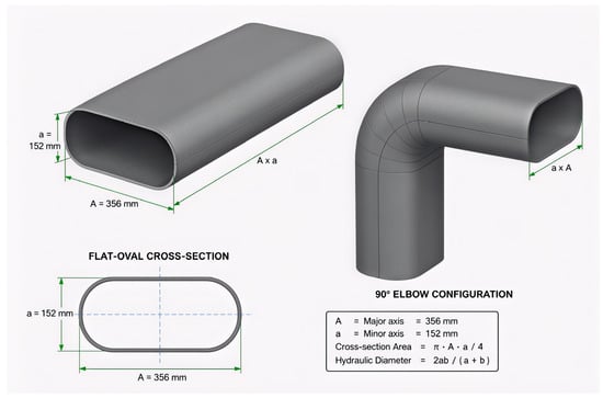
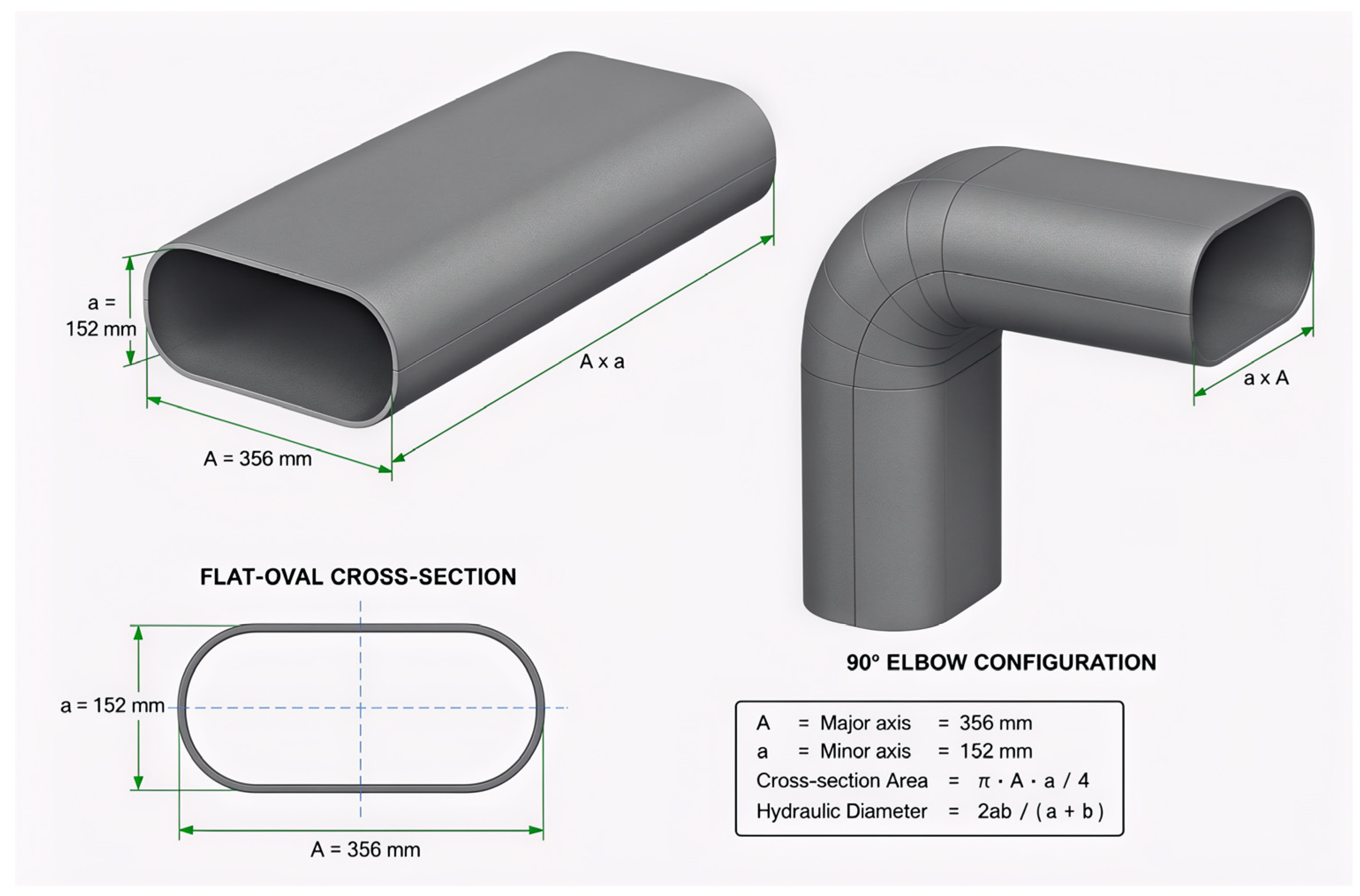
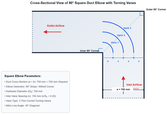
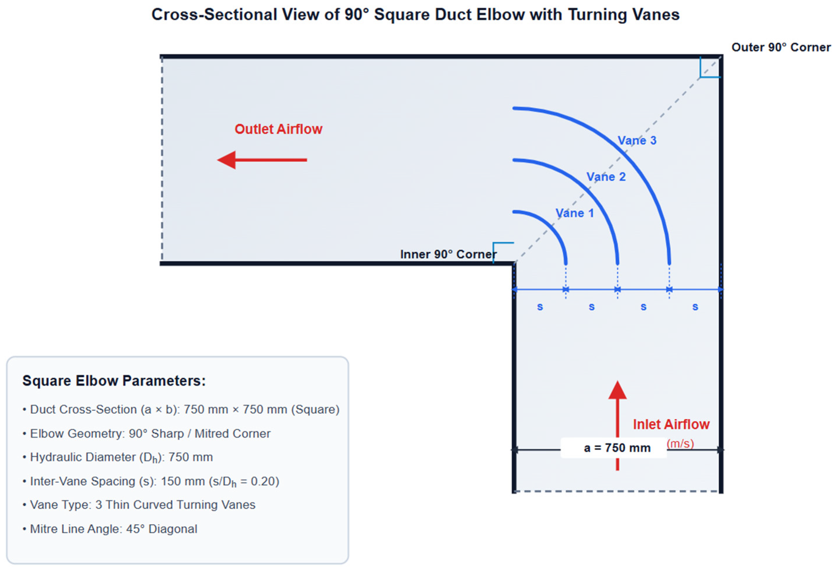
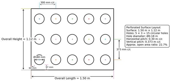
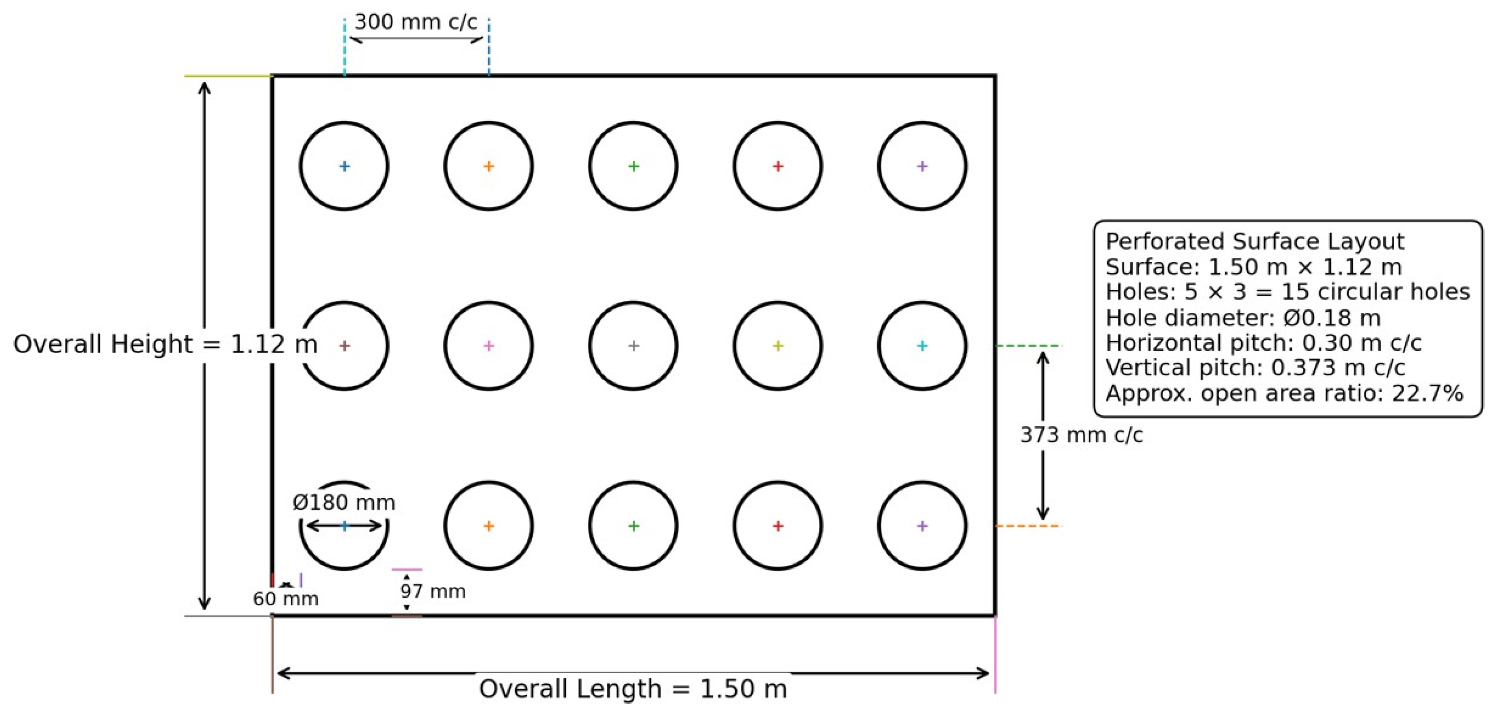
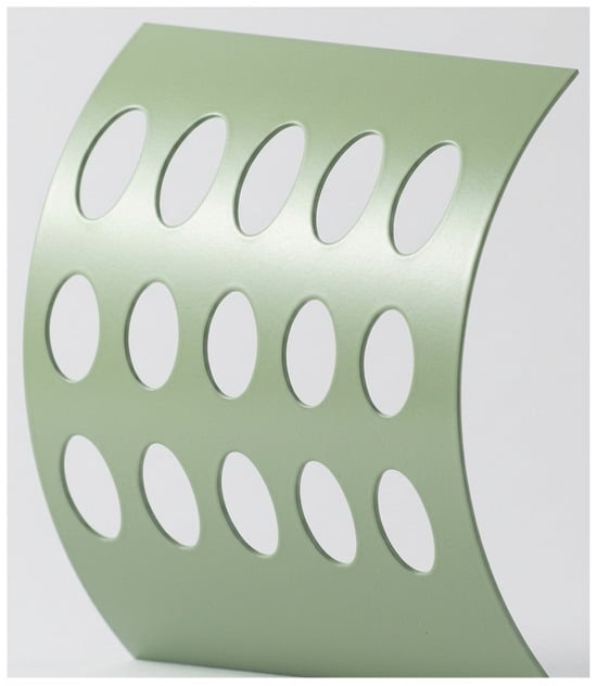
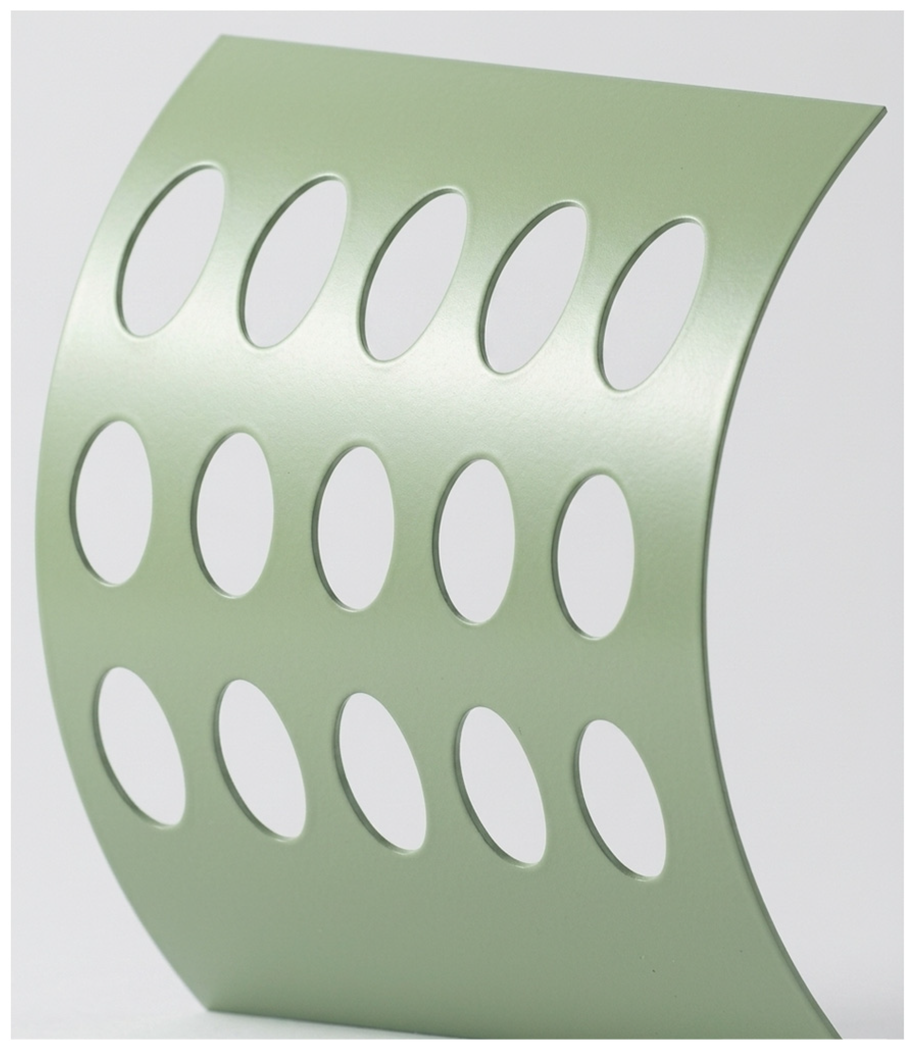
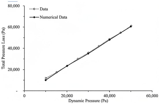
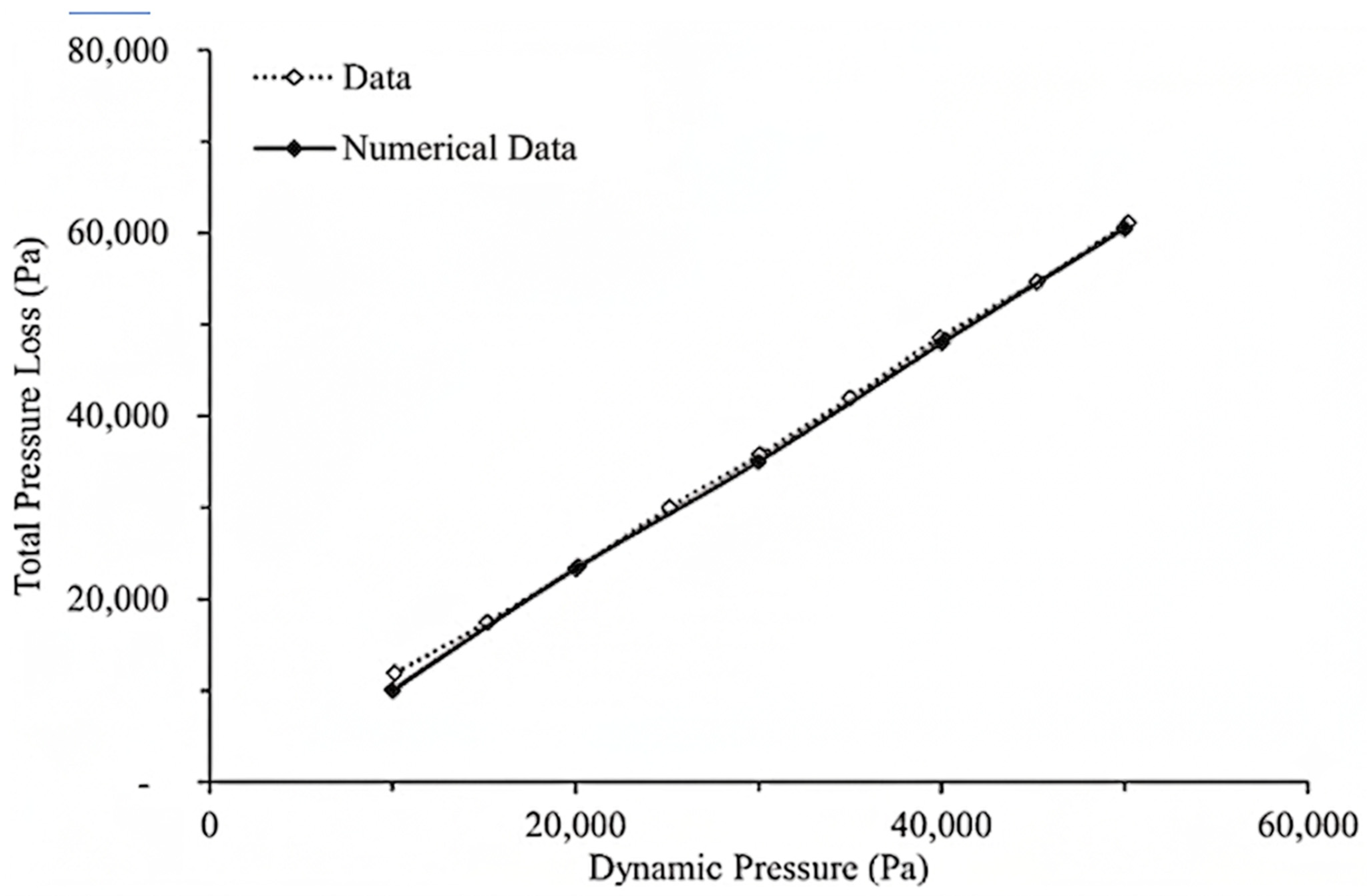
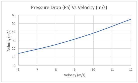
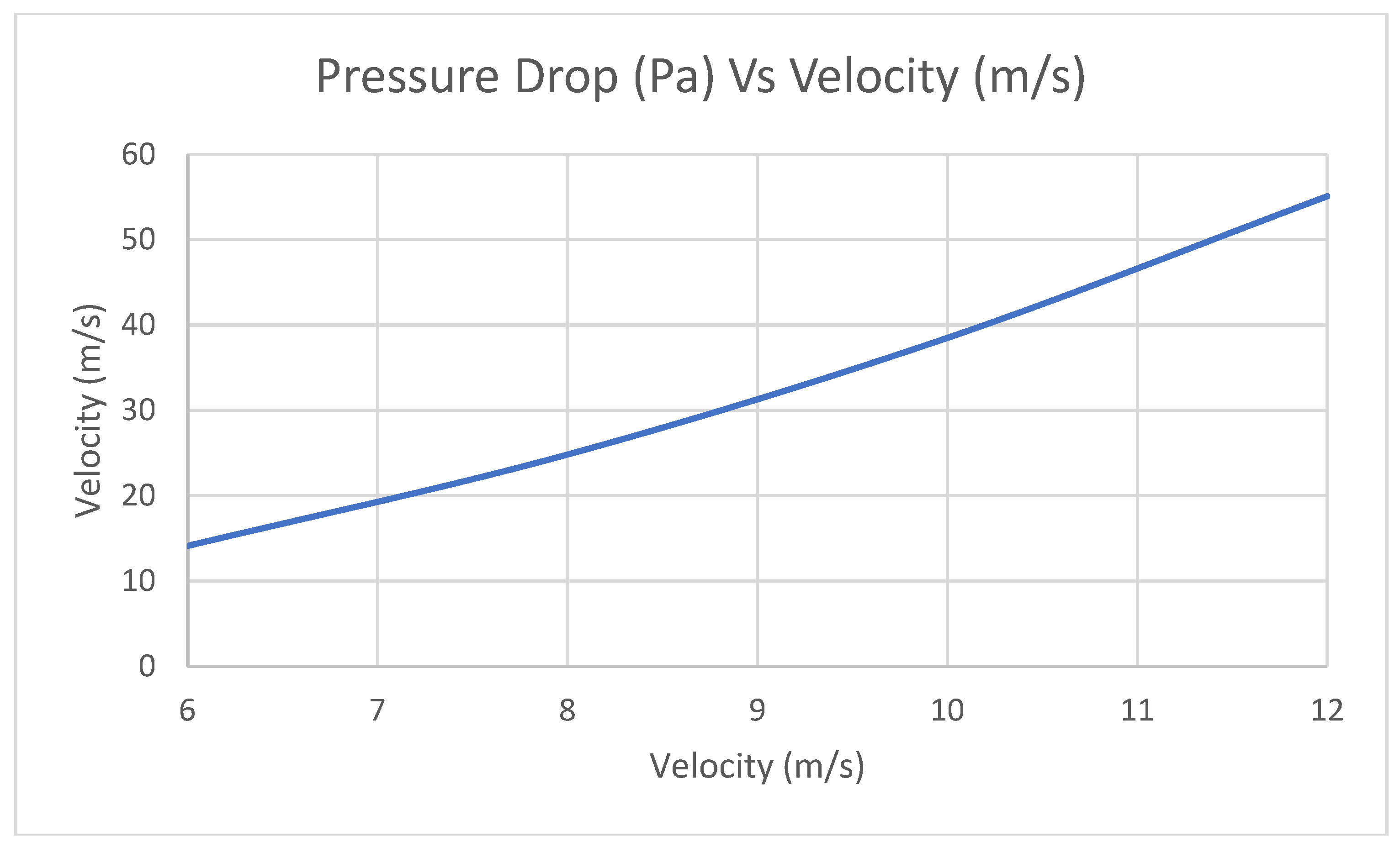
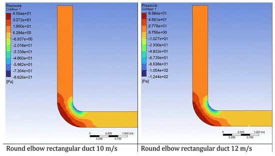
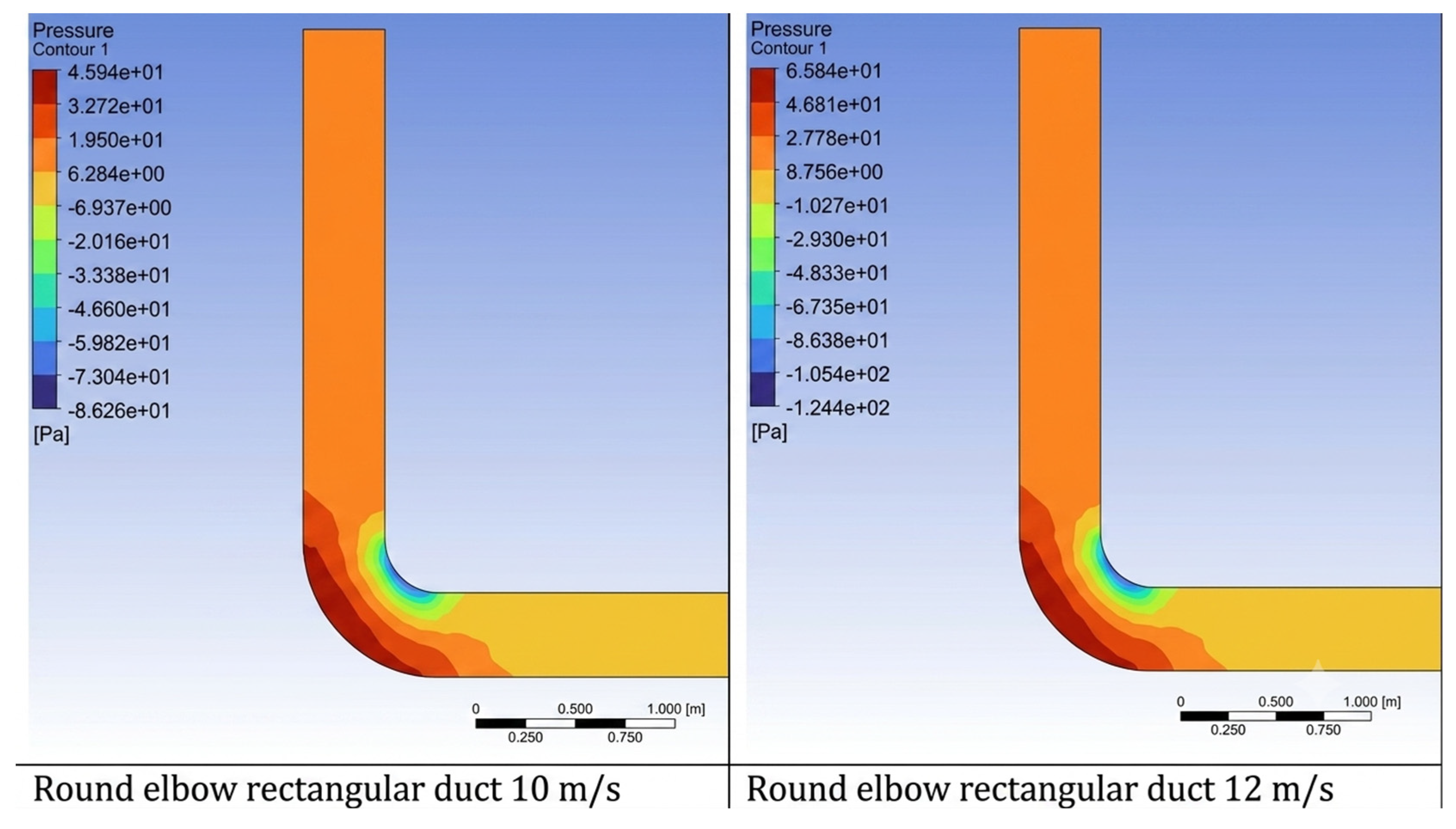
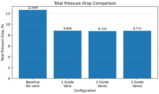
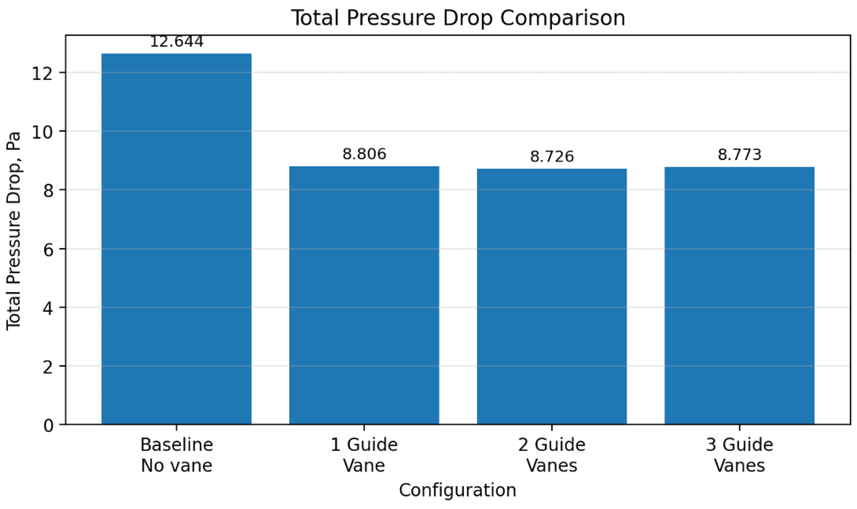
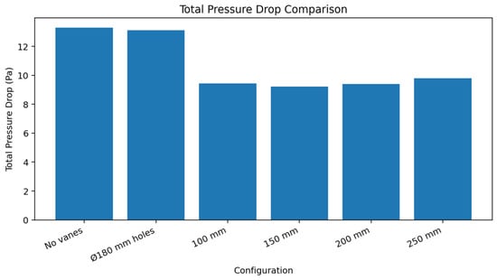
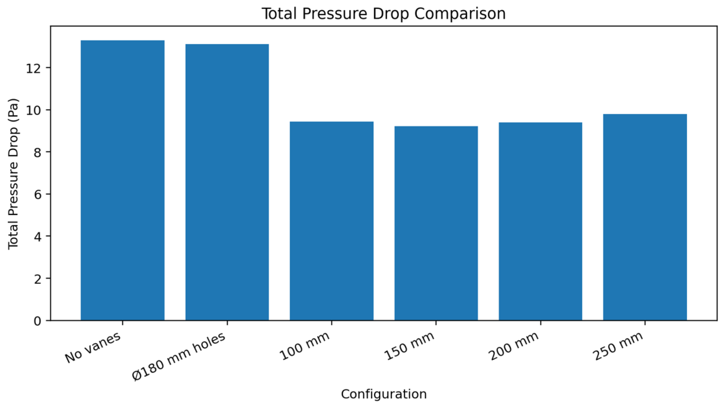
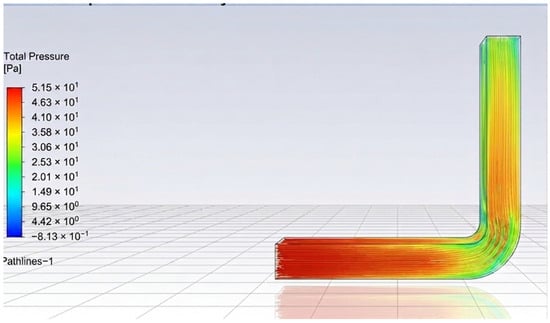
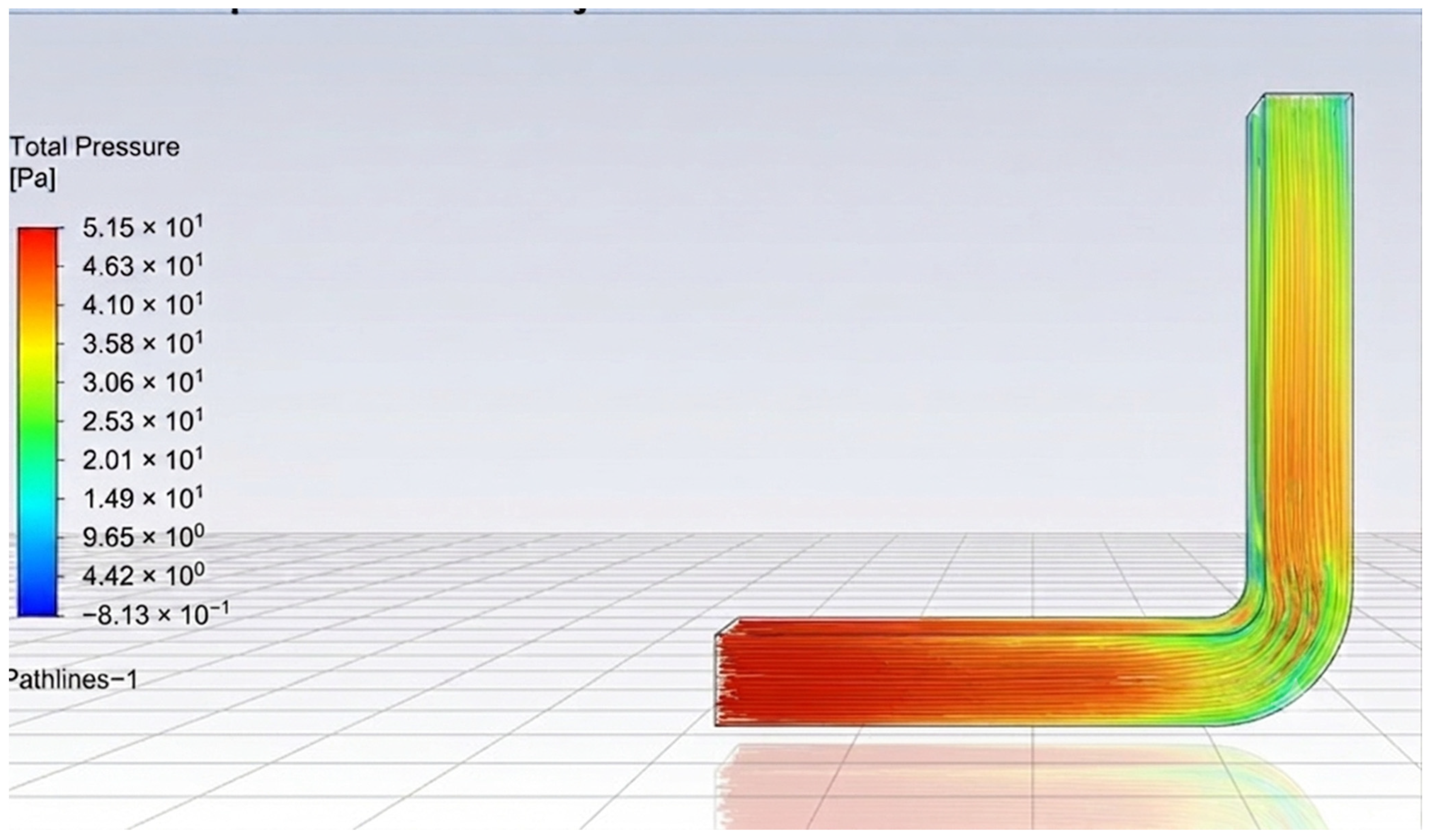
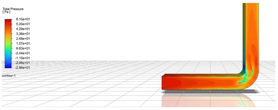
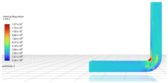

Disclaimer/Publisher’s Note: The statements, opinions and data contained in all publications are solely those of the individual author(s) and contributor(s) and not of MDPI and/or the editor(s). MDPI and/or the editor(s) disclaim responsibility for any injury to people or property resulting from any ideas, methods, instructions or products referred to in the content. |
© 2026 by the authors. Licensee MDPI, Basel, Switzerland. This article is an open access article distributed under the terms and conditions of the Creative Commons Attribution (CC BY) license.