Physics-Driven Parameter Identification for High-Fidelity Extraction of Spindle Static Nonlinear Axial Stiffness

Abstract

The nonlinear operational stiffness characteristics of machine tool spindles directly influence machining precision and bearing service life. Traditional static stiffness tests rely on direct differential operations on raw experimental load–displacement data, which are highly susceptible to measurement noise and fundamentally fail to capture accurate nonlinear features. To address this limitation, this study proposes a physics-driven parameter identification methodology to accurately extract the static nonlinear axial stiffness characteristics of spindles under static non-rotating conditions. Specifically, the smoothness priors approach (SPA) is introduced as a robust preprocessing technique to mitigate high-frequency noise while preserving the underlying low-frequency displacement trends, thereby ensuring high-fidelity feature extraction. Subsequently, a physics-dependent spindle mechanics model is directly integrated with a two-stage hybrid optimization algorithm—combining Global Search and Pattern Search—to inversely reconstruct the actual nonlinear load–displacement relationships. Numerical simulation results demonstrate that the hybrid optimization algorithm exhibits high computational accuracy, with an identification error of only 0.67% under ideal conditions and bounded parameter identification errors within 4.68% under synthetic noise levels up to 5%. Furthermore, experimental validation conducted on a position-preloaded spindle setup under initial preloads of 507 N and 862 N yields corresponding verification errors of 12.3% and 11.6%, respectively, confirming that the proposed method can effectively extract the static nonlinear stiffness features of the spindle from noisy measurements. The results demonstrate that this approach successfully overcomes the bottlenecks of conventional techniques, providing a robust and practical tool for the precise characterization of the spindle’s static nonlinear baseline stiffness. While currently validated under static non-rotating conditions, the established framework provides a fundamental baseline for extending parameter identification to dynamic operational environments in future studies.

1. Introduction

High-speed machining and high-precision machining are core long-term trends in modern manufacturing, where the high-performance capabilities of the machine tool spindle are a key prerequisite [1,2,3]. Spindle stiffness, as one of the primary indicators for evaluating and analyzing spindle service performance, has gained widespread attention [4]. With the rapid integration of Industry 4.0 paradigms, contemporary spindle condition evaluation has expanded into advanced architectures, such as physics-informed parameter identification, digital twins, and data-driven condition monitoring, to trace structural integrity and stiffness degradation in real time [5,6,7]. To further enhance diagnosis reliability and condition monitoring, recent international studies have proposed advanced hybrid physics and data-driven frameworks specifically tailored for spindle fault detection and health diagnosis [8,9]. In practical engineering applications, angular contact ball bearings within the spindle exhibit highly nonlinear stiffness characteristics due to complex contact mechanics and internal preloads [10]. Insufficient spindle stiffness not only readily produces chatter, excessive tool tilt, and unwanted back cutting, compromising machining precision, but also causes rolling element slippage, increasing bearing wear and reducing spindle life [4]. As a result, the effective evaluation and maintenance of spindle stiffness have long been key concerns in the machine tool industry.

Static stiffness, which characterizes the ability of the spindle to resist deformation under constant or quasi-static load, has a significant impact on the dimensional and geometric accuracy of the machined workpiece. To evaluate this indicator, researchers have developed various numerical and experimental methods. Cun [11] and Cui [12] constructed spindle bearing finite element models to simulate static stiffness, validating them experimentally via mechanical loading devices. Bardac [13] employed the finite element approach to examine the static stiffness of CNC turning spindles for structural design optimization. With the aid of strain testers and force transducers, Huang [14] and Liu [15] established static stiffness test platforms to explore the relationship between spindle static stiffness and applied loads. In the existing literature, the academic and industrial communities have generally employed direct numerical differentiation to process load–displacement curves for the extraction of stiffness characteristics. However, a critical limitation of these traditional measurement approaches—as illustrated in previous comparative studies [16]—is that they fit a straight line to representative data or compute an average slope, treating spindle stiffness as a linear constant value and fundamentally lacking the concept of stiffness nonlinearity. In contrast to these simplified views, true spindle operational behaviors exhibit a pronounced, full-cycle nonlinear evolution where the stiffness values continuously vary with displacement across the entire loading range, rather than remaining constant or only demonstrating localized variations during bearing unloading [16]. Although recent high-level publications have leveraged nonlinear dynamic analysis, thermo-solid coupling simulations, and equivalent nonlinear material back-calculation to analyze bearing contact mechanics under varying conditions [17,18,19], bridging the gap between theoretical multi-parameter modeling and high-fidelity empirical continuous stiffness extraction remains an unresolved challenge. The consequence of neglecting this nonlinearity is profound: in precision heavy-duty machining or variable-load cutting processes, treating stiffness as a linear constant leads to a severe mismatch between theoretical models and actual spindle deformations, causing uncontrollable structural vibrations and instability [1]. Crucially, as the external cutting force increases to a critical threshold, the bearing on the non-loading side shifts into an “unloading state” [16,20]. At this inflection point, the spindle’s localized stiffness undergoes a drastic, non-smooth drop. If this nonlinear sudden mutation is overlooked during testing, the mechanical system will fail to safely predict the spindle’s critical bearing capacity and risk abrupt structural failure under extreme conditions. Therefore, accurately tracking the continuous evolution of nonlinear stiffness and identifying the precise boundaries of bearing unloading states is an absolute necessity for structural safety margin evaluation and active vibration control in high-end machine tools [21].

To accurately back-calculate operational parameters from theoretical architectures, various optimization-based inverse modeling and physics-informed parameter identification frameworks have emerged in recent years. Notably, recent global advancements in digital twin technologies have successfully utilized inverse mapping models and Bayesian frameworks for the real-time parameter updating and uncertainty quantification of complex nonlinear dynamical systems [22,23]. Furthermore, hybrid frameworks combining multi-layer perceptrons with Bayesian optimization [24], 4-DOF dynamic models integrated with least-squares and Monte Carlo simulations [25], 2D thermomechanical finite element inverse design coupled with neural networks [26], and lumped parameter dynamics enhanced by transfer learning or genetic algorithms [27] have been successfully implemented to identify dynamic properties, bearing geometric variations, or fault states. However, a critical gap exists when comparing these existing algorithmic frameworks with the specific demands of nonlinear stiffness extraction. As highlighted in the literature, existing algorithms are predominantly data-driven black boxes or rely on pure mathematical curve-fitting. They are primarily tailored for structural design optimization, intelligent fault diagnosis, or discrete parameter tuning within localized boundaries. They do not explicitly distinguish or continuously reconstruct the full-period evolution of spindle operational stiffness across the entire load range from noisy experimental measurements. Crucially, because conventional optimization algorithms in the aforementioned literature lack explicit mechanical boundary constraints, they are fundamentally ill-equipped to handle the severe, non-smooth stiffness mutations induced by bearing unloading states. When traditional pure mathematical models attempt to fit these nonlinear mutations, they typically converge to physically impossible local minima or suffer from severe phase-dependent discrepancies, leaving a critical industry pain point unaddressed. To capture the real nonlinear behavior of spindle systems under quasi-static conditions, high-resolution load–displacement data must be collected continuously. Nevertheless, during the practical experimental testing of machine tool spindles, raw sampled data are highly susceptible to high-level noise induced by experimental system misalignments, flatness errors of the target disk, and electromagnetic interference during transmission. Because the mathematical differential operations required to calculate nonlinear stiffness are exceptionally sensitive to data fluctuations, conventional processing methods (such as direct differentiation) often lead to severe numerical divergence when facing noisy signals, causing the so-called “stiffness characteristics” to be completely submerged by noise. Accurately and robustly extracting nonlinear stiffness curves from raw measurements containing complex noise, especially capturing the stiffness mutations at bearing unloading states, remains a critical bottleneck problem in the field of spindle stiffness testing [19].

To address this fundamental limitation in the existing literature, this study proposes a novel experimental testing method to extract the continuous, full-cycle nonlinear axial stiffness characteristics of machine tool spindles based on a physics-driven parameter identification framework, explicitly separating its mechanism from traditional design optimization or discrete fault-tuning approaches. Unlike existing purely data-driven models, the proposed algorithm explicitly highlights its innovation through three detailed, mechanism-compliant optimization steps:

Step 1: Non-Distorting Noise Regularization via SPA. While traditional signal processing techniques such as Wavelet Transform (WT) and Empirical Mode Decomposition (EMD) have been widely utilized for noise reduction, they often suffer from phase distortion, mode mixing, or the risk of over-smoothing critical sudden mutations in non-stationary signals. To address this, the smoothness priors approach (SPA)—a well-established and robust regularization-based technique [28,29]—is adopted to preprocess the raw sampled data. This step strictly preserves the true underlying physical displacement trends and critical unloading phase boundaries without phase shifting, ensuring a high-fidelity data foundation.

Step 2: Physics-Driven Mechanism Embedding. Diverging from traditional black-box data fitting, the “physics-driven” core of this algorithm establishes an explicit mechanism-compliant model governed by Hertzian contact theory and spindle bearing kinematics. This step uniquely embeds hard physical boundary constraints—specifically the critical bearing unloading displacement thresholds (δ₁ and δ₂)—directly into the optimization loop, mapping raw signals to actual structural parameters and ensuring that the identified profiles strictly adhere to physical laws.

Step 3: Two-Stage Hybrid Optimization. To overcome the local minima entrapment and phase-dependent discrepancies prevalent in single-algorithm optimizations, a physics-dependent spindle mechanics model is integrated with a two-stage hybrid optimization algorithm—combining Global Search and Pattern Search [30]—to identify critical bearing internal parameters [31] and reconstruct the actual noise-free load–displacement relationship.

Through this physics-based parameter identification strategy, the proposed approach not only bypasses the stringent signal-to-noise ratio requirements of traditional differentiation but also provides a universal, highly robust technical pathway for revealing nonlinear stiffness behaviors under complex industrial conditions. It is worth noting that while the underlying spindle mechanics model explicitly accommodates the speed parameter n, the experimental validation in this study is intentionally conducted under static conditions (0 rpm) at a constant room temperature. This controlled environment is carefully selected as a fundamental benchmarking step to isolate and verify the core feature extraction capacity and noise immunity of the identification framework, thereby preventing the coupling of complex rotational vibrations and transient thermal drifts. The detailed dynamic impacts of operational speeds on spindle stiffness softening/hardening have been theoretically and experimentally explored in our previous work [20], while full-cycle thermomechanical coupling behaviors constitute our ongoing research. Finally, the finite difference method is applied to the reconstructed true values to reveal the clear nonlinear stiffness profiles and transition points.

2. Preliminary Framework for Spindle Stiffness Parameter Identification

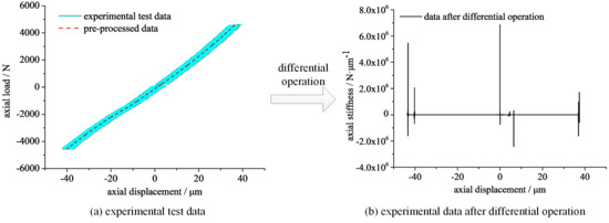
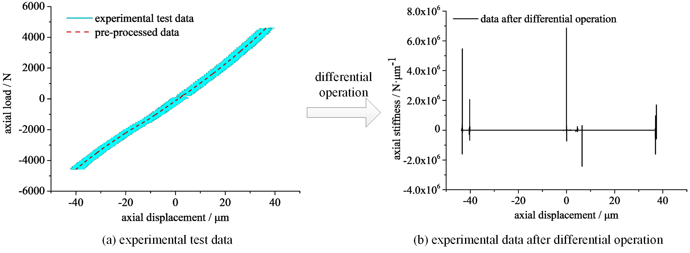
In the static stiffness test of a machine tool spindle, it is inevitable that the original test data will fluctuate relatively widely and the signal-to-noise ratio will be poor because of misalignments between the test equipment and the spindle under test, the flatness error of the displacement target disk and its perpendicularity error with the axial centerline of the spindle, the inevitable interference in the signal acquisition and transmission process, etc. In conventional testing approaches, single-point sensors are typically configured along a single measurement vector, causing geometric errors—such as target disk surface roughness, microscopic tilt, and assembly eccentricity—to couple directly into the raw displacement readings. Because the mathematical evaluation of continuous stiffness requires numerical differentiation (K = dF/dδ), these micro-level irregularities are multiplied by orders of magnitude through the derivative operator, leading to severe signal fluctuations and an extremely low signal-to-noise ratio (SNR) that completely submerges the true nonlinear evolution, as illustrated by the chaotic baseline in Figure 1b. To enhance methodological transparency and guarantee structural clarity from the outset, it is explicitly clarified that the raw experimental dataset presented in Figure 1 is acquired from the exact same position-preloaded spindle test rig detailed later in Section 4.1. Specifically, the tested spindle configuration consists of a pair of angular contact ball bearings (NSK 7014C) arranged back-to-back. The quasi-static axial force is applied via a bidirectional mechanical loading device equipped with an HBM force sensor, while the resulting displacement is synchronously captured by three high-precision eddy current sensors evenly distributed at 120° intervals around the target disk circumference to mathematically average out geometric runout. A comprehensive engineering schematic and physical layout of this experimental assembly are fully documented in Figure 12. Since the differential operation for solving the spindle stiffness is exceptionally sensitive to data fluctuations, it is difficult to solve the accurate stiffness value directly by using the difference operation. Consequently, data preprocessing is essential before spindle stiffness parameter identification. In this section, the preparatory work for spindle stiffness parameter identification is introduced: signal preprocessing and the spindle mechanics model (dependency model for stiffness parameter identification).

Figure 1. Limitations of direct numerical differentiation on raw experimental data: (a) measured load–displacement experimental curve with noise envelope; (b) axial stiffness obtained via direct numerical differentiation, showing severe noise amplification and divergence.

2.1. Signal Preprocessing

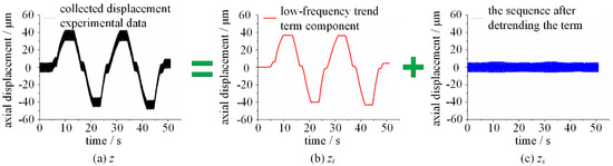
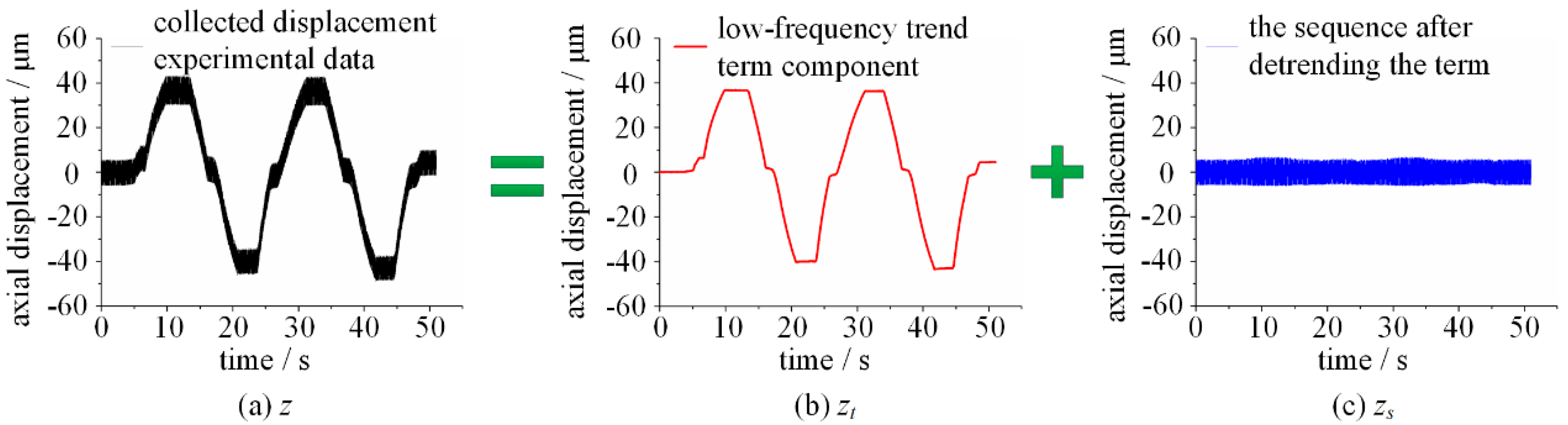
The true values of the axial displacement and axial load signals collected during the spindle axial stiffness test are low-frequency slow-varying signals. Based on the signal characterization, it can be assumed that the collected signals z can be divided into two parts (as shown in Figure 2).

$$z=z_t+z_s$$

(1)

where z_t denotes the low-frequency trend term component (which refers to the true value of the test signal in this study); z_s is the sequence after detrending the term (which can be interpreted as the noise interference signal in this paper).

Figure 2. Displacement signal decomposition via the smoothness priors approach (SPA): (a) raw signal Z; (b) extracted low-frequency trend Z_t; (c) detrended residual noise component Z_s.

For the signal to be processed during the spindle stiffness test, the trend term is the effective term of the signal to be processed, while the periodic term is the noise interference term to be filtered out from the signal to be processed. Therefore, with the help of the signal trend term elimination principle based on the smoothness priors approach [28,29], the purpose of filtering and noise elimination of the load and displacement signals collected can be achieved by retaining the trend term in the signal to be processed and removing the periodic term in the signal to be processed.

According to refs. [28,29], the low-frequency trend term z_t can be expressed as

$$\stackrel{\wedge }{z_t}=z{\left(I+{\lambda }^2{D}_2^T{D}_2\right)}^{-1}=Lz$$

(2)

where L acts as a time-varying finite impulse response low-pass filter whose frequency response can be adjusted by the regularization parameter λ to meet different filtering requirements. I denotes the unit matrix. D₂ is the second-order difference matrix, which can be derived from Equation (3).

$$D_2=\left(\begin{array}{cccccc}1& -2& 1& 0& \dots & 0\\ 0& 1& -2& 1& \ddots & ⋮\\ ⋮& \ddots & \ddots & \ddots & \ddots & 0\\ 0& \dots & 0& 1& -2& 1\end{array}\right)$$

(3)

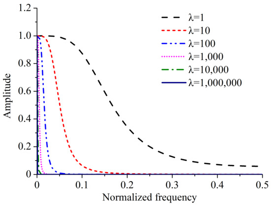
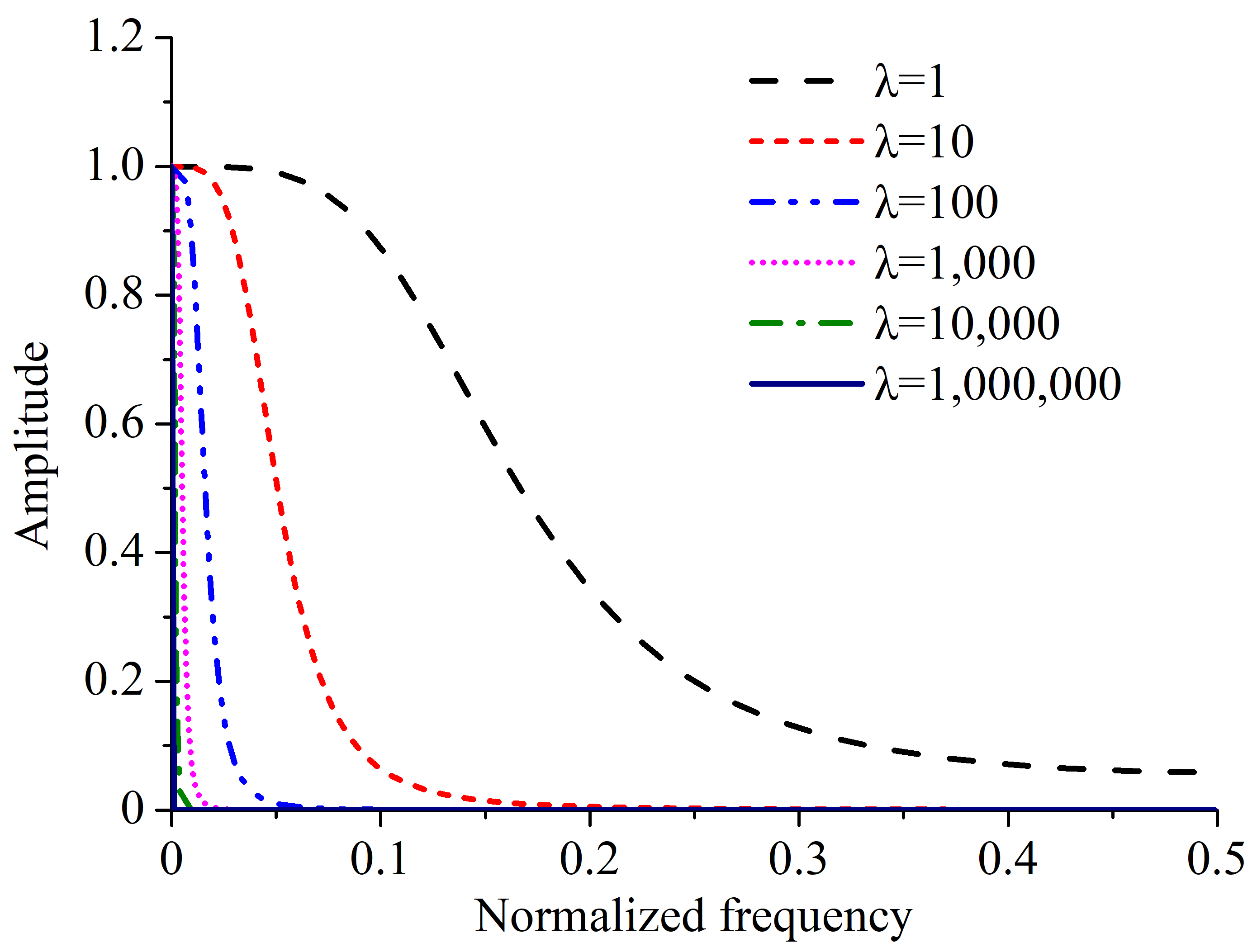
By assigning a value to the regularization parameter λ and applying a Fourier transform to row N/2 of L, the frequency response of different λ values can be obtained, and the results are shown in Figure 3. It can be seen that as the regularization parameter λ increases, the cutoff frequency of the “filter” decreases; i.e., the frequency component of the trend term extracted from the filtered signal is also lower.

Figure 3. Frequency response of the SPA low-pass filter under varying regularization parameters (λ = 1 to 1,000,000), illustrating progressive high-frequency noise attenuation.

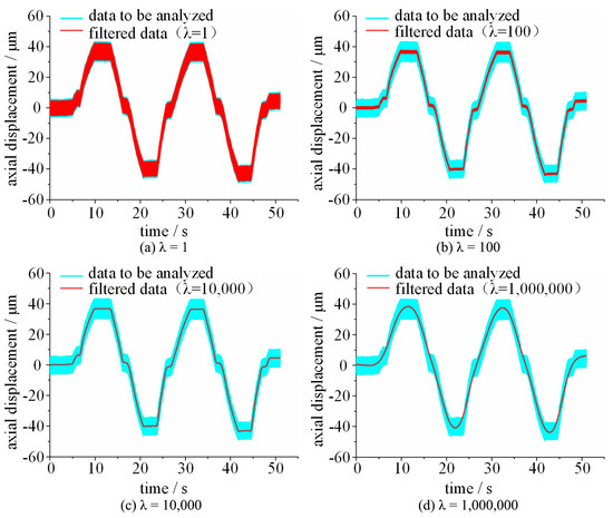
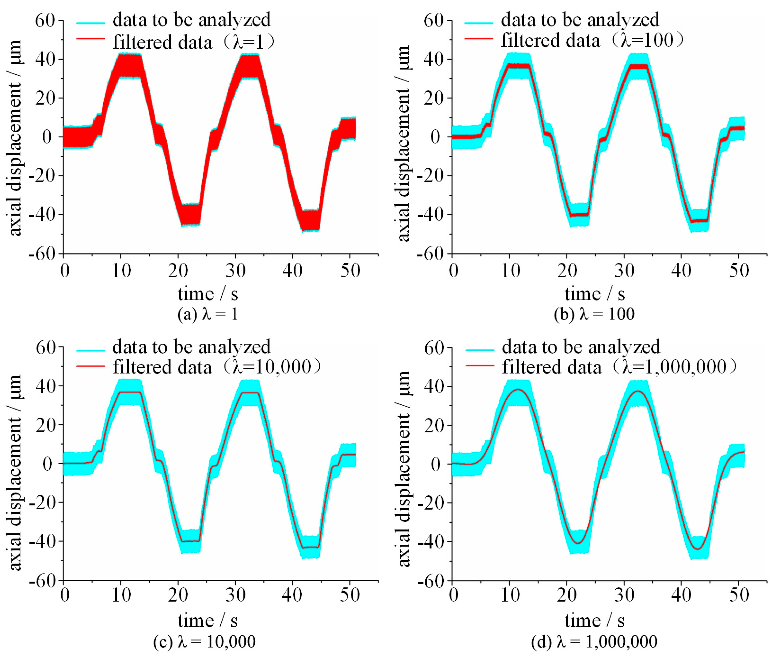
When using the smoothness priors approach to preprocess the displacement data collected during the spindle stiffness test, a comparison of the filtering effect of the signal is shown in Figure 4. As shown in Figure 4, with the gradual increase in the regularization parameter, the fluctuation of the extracted trend term components gradually decreases and the signal tends to be smoothed; i.e., the frequency in the low-frequency components contained in the extracted trend term gradually becomes lower, and the high-frequency components are successfully filtered out. For example, when the regularization parameter λ = 1, the difference between the maximum and minimum values of the fluctuation amplitude of the trend term components extracted from the original signal is 9.5 μm, while when the regularization parameter λ = 10,000, the maximum value of the fluctuation amplitude differs from the minimum value by only 0.07 μm. However, when λ = 1,000,000 (as seen in Figure 4d), the trend term extracted from the original signal reflects a certain deviation in regularity compared with the original signal, and the phenomenon of “over-filtering” appears. That is, when the value of the regularization parameter is too large, part of the effective information of the original signal may be filtered out, resulting in a lower resolution of the signal, which is not conducive to the improvement of the signal-to-noise ratio. Therefore, only when the corresponding cutoff frequency matches the frequency characteristics of the target signal can the effective components of the signal be retained as much as possible while the high-frequency noise interference can be efficiently filtered, and the signal-to-noise ratio of the signal can be effectively improved. To avoid relying primarily on qualitative visual observations, an objective selection criterion based on the L-curve method is introduced to optimize the regularization parameter λ. Specifically, the optimal λ is determined by balancing the trade-off between the roughness of the trend term (defined by the second-order difference norm ${‖D_2{z}_t‖}^2$) and the residual norm of the detrended noise component (${‖z-z_t‖}^2$). By plotting the log–log curve of these two metrics across a candidate set of λ ∈ [1, 10⁶], the optimal regularization parameter is mathematically identified at the distinct “inflection point” (maximum curvature) of the L-curve, where the noise suppression and signal fidelity reach an objective equilibrium. It is worth noting that standard preprocessing techniques, such as conventional low-pass Butterworth filters or cubic spline smoothing, present distinct limitations in this specific application. Conventional Butterworth filters inherently introduce phase lag and transient boundary distortions, which can artificially shift or blur the exact location of the highly sensitive stiffness inflection points (bearing unloading states). Meanwhile, cubic spline smoothing is highly sensitive to boundary conditions and knot placement, posing a substantial risk of over-smoothing the localized structural sudden mutations characteristic of bearing unloading. In contrast, SPA operates as a regularized matrix-based smoother that guarantees zero phase shift and optimally balances global smoothness with local trend fidelity through an automated L-curve selection, making it highly suitable for preserving sharp physical transition boundaries. A more comprehensive, quantitative benchmark of various signal processing algorithms for spindle stiffness identification will be prioritized in our future research. When using the trend term extraction method based on the smoothness priors method for signal preprocessing, attention should be paid to the selection of the regularization parameter λ in the algorithm. First, perform a Fourier transform on the signal to be analyzed to analyze the frequency composition of the signal. Then, determine the frequency range of the filtered target signal according to the frequency components of the signal to be analyzed. Finally, determine the cutoff frequency of the filter according to the frequency of the target signal, and select an appropriate regularization parameter λ based on Figure 3.

Figure 4. Filtering performance on raw displacement data across regularization parameters: (a) λ = 1 (under-filtered); (b) λ = 100 (partially filtered); (c) λ = 10,000 (optimal smoothing); (d) λ = 1,000,000 (over-filtered with phase delay).

2.2. Spindle Mechanics Model

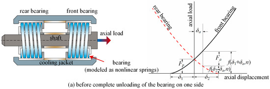
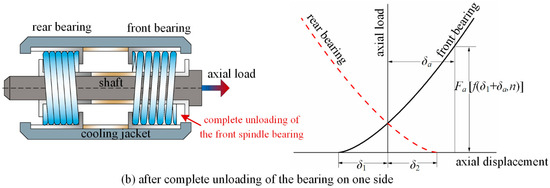
To establish a rigorous physical mapping of the investigated spindle architecture, a comprehensive schematic diagram illustrating the spindle mechanical configuration under axial tension/compression alongside its internal bearing force balance is presented in Figure 5. Unlike traditional empirical data-fitting or pure black-box approaches, the core philosophy of this framework is fundamentally “physics-driven.” It establishes an explicit mechanism-compliant dependence model governed by Hertzian contact theory and bearing kinematics (Equations (10)–(13)). Within this architecture, exact physical boundaries—specifically the critical displacement thresholds (δ₁,δ₂) that dictate the complete unloading states of the bearings—are directly embedded into the optimization loop as hard boundaries and search-trajectory guides.

Figure 5. Mechanical force equilibrium during bearing unloading: (a) coupled state before front bearing unloading; (b) uncoupled state after complete front bearing unloading.

To ensure computational tractability while maintaining high fidelity, several foundational assumptions are introduced to this spindle mechanics model: (1) the structural housing and the shaft are assumed to be rigid bodies relative to the highly flexible, nonlinear bearing contact zones; (2) the angular contact ball bearings undergo pure quasi-static elastic deformation without macroscopic structural wear or surface degradation; (3) the initial thermal equilibrium remains invariant during a single quasi-static static loading cycle. These boundary assumptions inherently introduce certain limitations: neglecting the structural compliance of the housing may cause a slight overestimation of the absolute system stiffness, while omitting transient thermal variations restricts the framework from capturing real-time thermal-preload mutations without localized baseline recalibration. Nevertheless, these mechanism constraints are indispensable; they prevent the optimization algorithm from converging toward mathematically valid but physically impossible local minima, guaranteeing that the identified parameters strictly adhere to real-world mechanical bounds.

To explicitly construct these physical bounds and guarantee full mathematical self-containment and computational reproducibility, the foundational contact mechanics and force equilibrium governing a single angular contact ball bearing are detailed below.

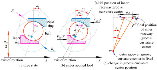
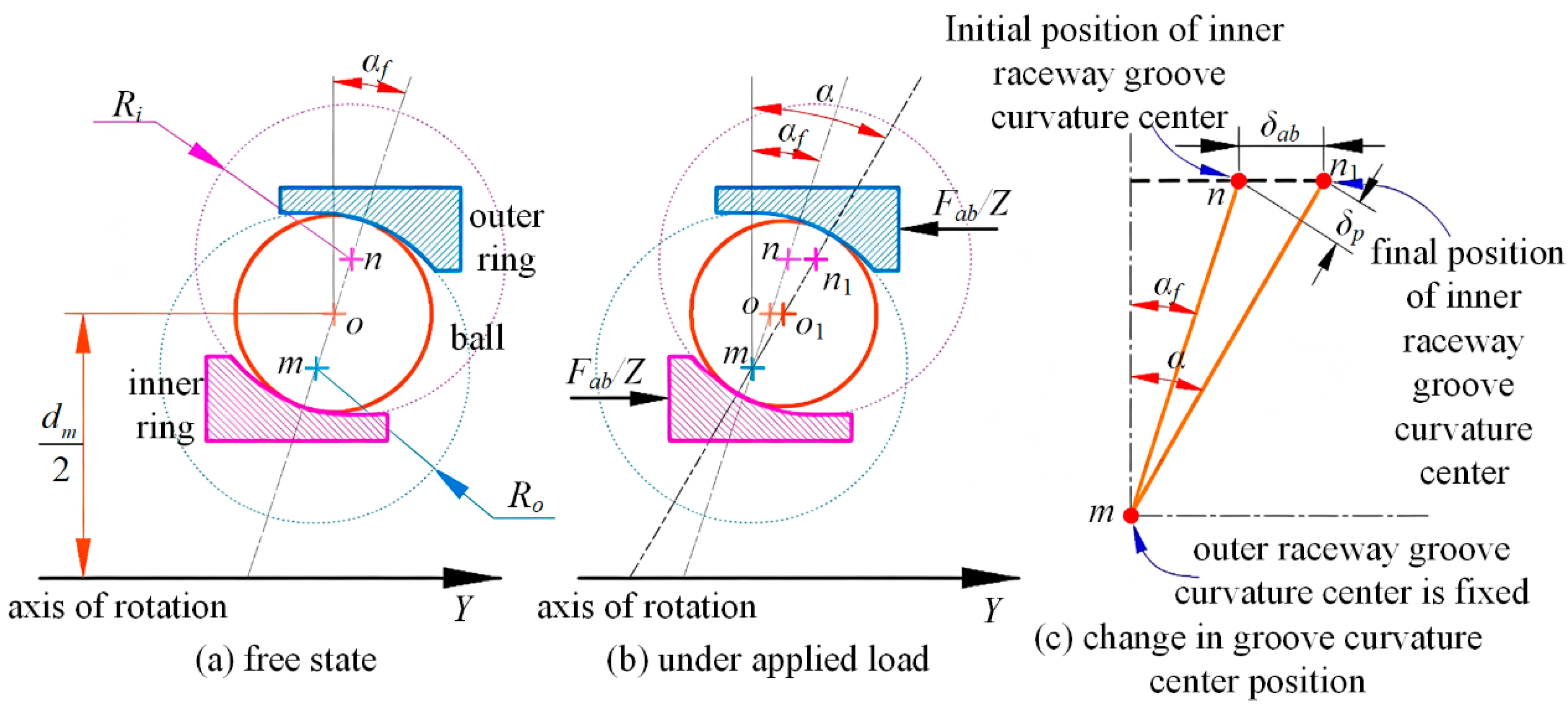
A schematic representation of the internal contact geometry and kinematic parameter relationships for an angular contact ball bearing subjected to axial deformation is illustrated in Figure 6. The initial distance between the curvature centers of the inner and outer raceway grooves, A₀, is expressed as

$$A_0=R_i+R_o-D_b=\left(f_i+f_o-1\right)D_b$$

(4)

where R_i and R_o denote the raceway groove curvature radii of the inner and outer rings, respectively; f_i and f_o are the non-dimensional groove curvature coefficients; and D_b represents the rolling element (ball) diameter.

Figure 6. Kinematics and contact geometry of an angular contact ball bearing under axial load: (a) free state; (b) loaded state under axial force F_ab; (c) locus shift of the inner raceway curvature center.

When relative axial displacement δ_ab occurs across the bearing, the spatial locus of the raceway groove curvature centers shifts. Based on the geometric trigonometry of the deformed state, the contact angle α under quasi-static equilibrium is mathematically calculated as

$$\alpha =\arcsin \left({\displaystyle \frac{A_0\sin {\alpha }_f+{\delta }_{ab}}{\sqrt{A_0^2{\cos }^2{\alpha }_f+{\left(A_0\sin {\alpha }_f+{\delta }_{ab}\right)}^2}}}\right)$$

(5)

where α_f denotes the initial unloaded contact angle.

According to Hertzian point contact theory, the overall elastic deflection load constant of the bearing, K_f, is determined by synthesizing the individual contact stiffness coefficients of the inner (k_i) and outer (k_o) raceways:

$$K_f={\left(k_i^{-\raisebox{1ex}{$2$}\!\left/ \!\raisebox{-1ex}{$3$}\right.}+k_o^{-\raisebox{1ex}{$2$}\!\left/ \!\raisebox{-1ex}{$3$}\right.}\right)}^{\raisebox{1ex}{$-3$}\!\left/ \!\raisebox{-1ex}{$2$}\right.}$$

(6)

The raceway contact deflection coefficients k_o and k_i are explicitly computed via

$$k_o=0.5973\cdot {\left({\displaystyle \frac{{\rho }_{2o}}{{\rho }_{1o}}}\right)}^{0.345}\cdot {\rho }_{2o}^{-0.5}{E}_o^{*}$$

(7)

$$k_i=0.5973\cdot {\left({\displaystyle \frac{{\rho }_{2i}}{{\rho }_{1i}}}\right)}^{0.345}\cdot {\rho }_{2i}^{-0.5}{E}_i^{*}$$

(8)

where ρ_1i, ρ_2i, ρ_1o, and ρ_2o represent the principal curvatures of the contact ellipses at the inner and outer raceway interfaces, while E_i^* and E_o^* represent the equivalent elastic moduli of the contacting materials.

By integrating the elastic Hertzian contact restoring forces across all Z active rolling elements along the axial direction, the total axial load F_ab developed by a single bearing as a function of axial displacement δ_ab is explicitly formulated as

$$F_{ab}=Z{K}_f{A}_0^{1.5}\sin \alpha {\left({\displaystyle \frac{\cos {\alpha }_f}{\cos \alpha }}-1\right)}^{1.5}$$

(9)

Equations (4)–(9) explicitly define the single-bearing contact statics. For concise notation in subsequent system-level equilibrium modeling, this nonlinear force–displacement relationship is compactly represented as

$$F_{ab}=f\left({\delta }_{ab}\right)$$

(10)

The loading process can be divided into three stages.

The first stage is the initial stage; under the action of the initial preload F_p, the pre-deflections of the front and rear bearings are δ₁ and δ₂, respectively. At this time, the spindle rotates smoothly without any external load, and the load distribution of the front and rear bearings satisfies the following relationship:

$$F_p=f\left({\delta }_1\right)=f\left({\delta }_2\right)$$

(11)

The second stage is the tension-bearing stage; at the beginning of this stage, the tensile force is small, and at this time, the spindle axial displacement δ_a is less than the bearing pre-deflection δ₂ (assuming that the spindle bearings are mounted back-to-back), and the tensile load is shared by the front and rear bearings. With an increase in tension, when the axial displacement δ_a is greater than the bearing pre-deflection δ₂, one side of the bearing is completely unloaded, and then the axial load is completely borne by the other side of the bearing. The spindle load distribution can be described as

$$\left\{\begin{array}{cc}f\left({\delta }_1+{\delta }_a\right)=F_a+f\left({\delta }_2-{\delta }_a\right)\hfill & \hspace{1em}\hspace{1em}{\delta }_a<{\delta }_2\hfill \\ f\left({\delta }_1+{\delta }_a\right)=F_a\hfill & \hspace{1em}\hspace{1em}{\delta }_a\ge {\delta }_2\hfill \end{array}\right.$$

(12)

The third stage is the compression-bearing stage, and the analysis principle of the compression-bearing stage is completely similar to that of the tension-bearing stage. At the beginning of the compression-bearing stage, the compressive load is completely shared by the front and rear bearings. With a further increase in compression, the bearing on one side of the spindle is completely unloaded and the compressive load is borne by the bearing on the other side alone. The spindle load distribution can be expressed as

$$\left\{\begin{array}{cc}{F}_a+f\left({\delta }_1-{\delta }_a\right)=f\left({\delta }_2+{\delta }_a\right)\hfill & \hspace{1em}\hspace{1em}{\delta }_a<{\delta }_1\hfill \\ F_a=f\left({\delta }_2+{\delta }_a\right)\hfill & \hspace{1em}\hspace{1em}{\delta }_a\ge {\delta }_1\hfill \end{array}\right.$$

(13)

Specifically, the transition boundary to the unloading state (the second and third stages) is governed by a critical axial displacement criterion; i.e., the axial displacement δ_a equals the bearing pre-deflection δ₁ or δ₂. Once this mathematical threshold is crossed (δ_a ≥ δ₂ or δ_a ≥ δ₁), the localized stiffness matrix component of the unloaded bearing abruptly drops to zero, transferring the entire load sequence to a single bearing. This discontinuous jump in the mathematical model is the fundamental physical origin of the nonlinear stiffness mutation observed in the experiments.

Equations (10)–(13) constitute the baseline mechanics model of the fixed-position preload spindle, providing the theoretical dynamic relationship for bearing static stiffness parameter identification.

To quantitatively account for the structural compliance of surrounding components (including shaft bending, axial housing compliance, and test rig interface elasticity) without losing computational tractability, a classical series structural elasticity coupling framework is incorporated into the mechanics baseline. The total measured macroscopic axial compliance C_sys captured by the displacement sensors at the spindle nose is expressed as a series spring combination:

$$C_{sys}\left(F_a\right)=C_b\left(F_a\right)+C_{struct}={\displaystyle \frac{1}{K_b\left(F_a\right)}}+C_{struct}$$

(14)

where K_b(F_a) represents the pure nonlinear contact stiffness of the angular contact ball bearing pairs derived from Hertzian contact theory (Equations (4)–(10)), and C_struct denotes the equivalent linear compliance of the unmodeled surrounding structural components (C_struct = 1/K_struct). Consequently, the identified spindle system axial stiffness K_id(F_a) extracted from sensor displacement measurements relates to the pure bearing contact stiffness K_b(F_a) via

$$K_{id}\left(F_a\right)={\displaystyle \frac{1}{C_{sys}\left(F_a\right)}}={\displaystyle \frac{K_b\left(F_a\right)}{1+K_b\left(F_a\right)\cdot C_{struct}}}$$

(15)

3. Spindle Static Stiffness Nonlinear Characteristic Extraction Method

3.1. Principle and Workflow

In order to effectively extract the nonlinear characteristics of spindle static stiffness, an experimental measurement method of spindle static stiffness based on parameter identification is proposed in this paper. The basic principle of parameter identification is to determine a set of parameter values based on the measured data and the theoretical model, so that the numerical results calculated by the theoretical model can best fit the measured data, then identify the true value of the test data, and finally solve the spindle stiffness based on the identified true value of the signal by a differential operation.

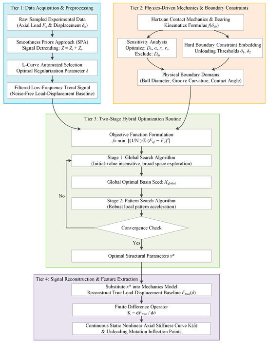
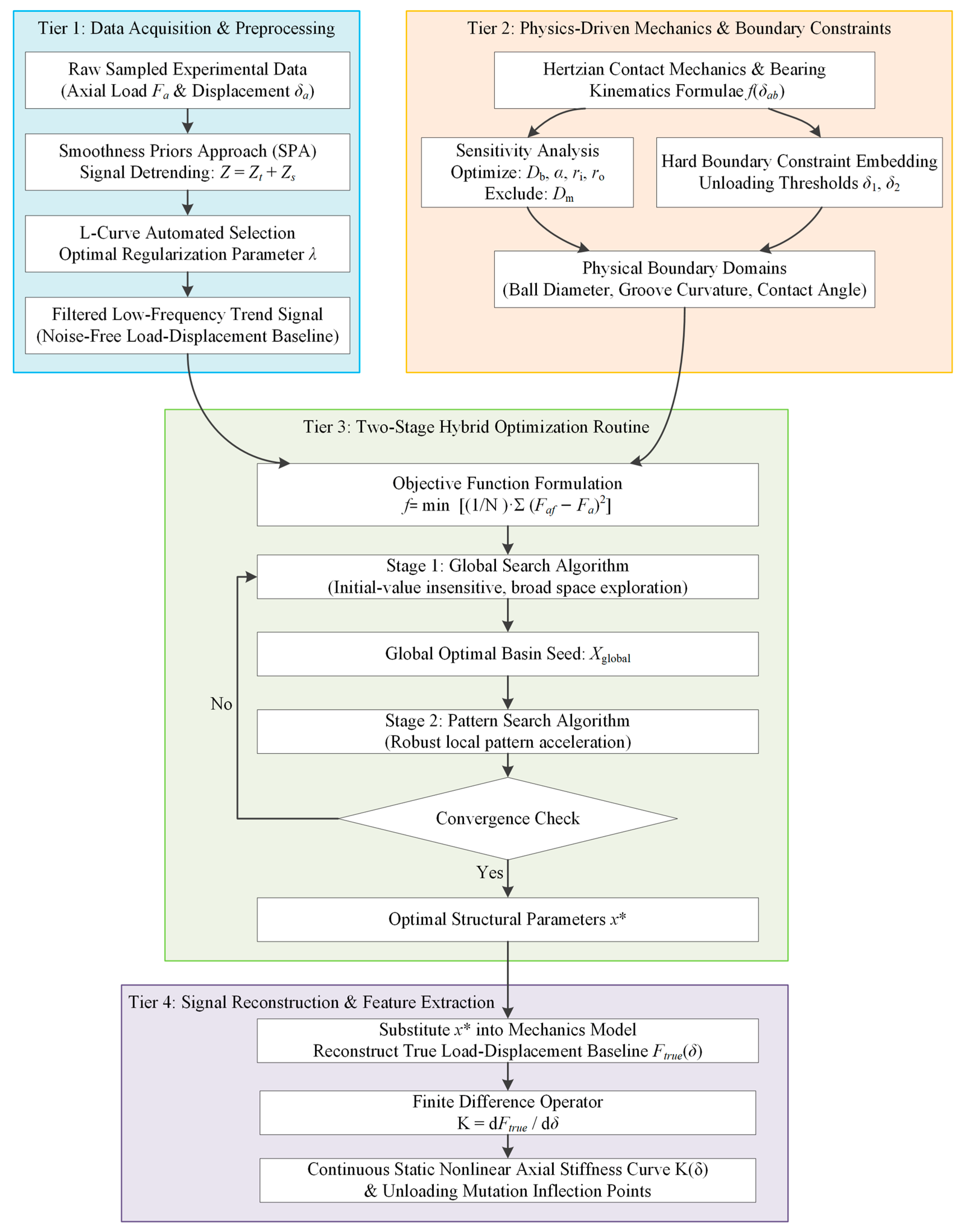
To provide complete methodological transparency and move beyond a generic algorithmic architecture, the detailed, physics-driven multi-stage workflow of the proposed parameter identification framework is explicitly structured and illustrated in Figure 7. The detailed execution protocol is decomposed into four sequential functional tiers: (1) Data Acquisition & Objective Preprocessing Tier: Raw load–displacement experimental data are collected synchronously from multi-channel eddy current sensors. To eliminate high-frequency shop-floor noise without inducing phase distortion, the smoothness priors approach (SPA) is applied, where the optimal regularization parameter λ is objectively determined via the automated L-curve inflection criterion. (2) Physics-Driven Mechanics Initialization Tier: Unlike black-box data-driven routines, this tier establishes an explicit mechanism-compliant model governed by Hertzian contact theory and bearing kinematics. Hard boundary constraints—specifically the critical bearing unloading displacement thresholds (δ₁ and δ₂) derived from equilibrium equations (Equations (10)–(13))—are embedded directly into the loop to serve as trajectory guides. (3) Two-Stage Hybrid Optimization Tier: To prevent local minima entrapment and phase-dependent discrepancies, the optimization loop is sequentially executed in two stages. First, the Global Search algorithm comprehensively explores the global parameter space (ball diameter, contact angle, and raceway groove curvature radii) with initial-value insensitivity. The resulting optimal spatial basin is subsequently fed as the rigorous initial seed into the Pattern Search algorithm for robust local fine-tuning. (4) Post-Processing & Stiffness Reconstruction Tier: Upon achieving convergence criteria, the optimal structural parameters are substituted back into the mechanics model to reconstruct the noise-free load–displacement true values. Finally, the finite difference method is applied to extract the continuous, full-cycle static nonlinear axial stiffness profiles K(δ) and pinpoint the critical bearing unloading inflection points.

Figure 7. Workflow of the physics-driven spindle parameter identification framework, structured into four modules: Module 1 (data preprocessing), Module 2 (bearing mechanics), Module 3 (two-stage hybrid optimization), and Module 4 (stiffness reconstruction).

3.2. Optimization Parameter Determination

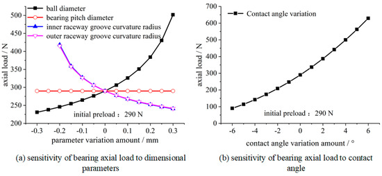
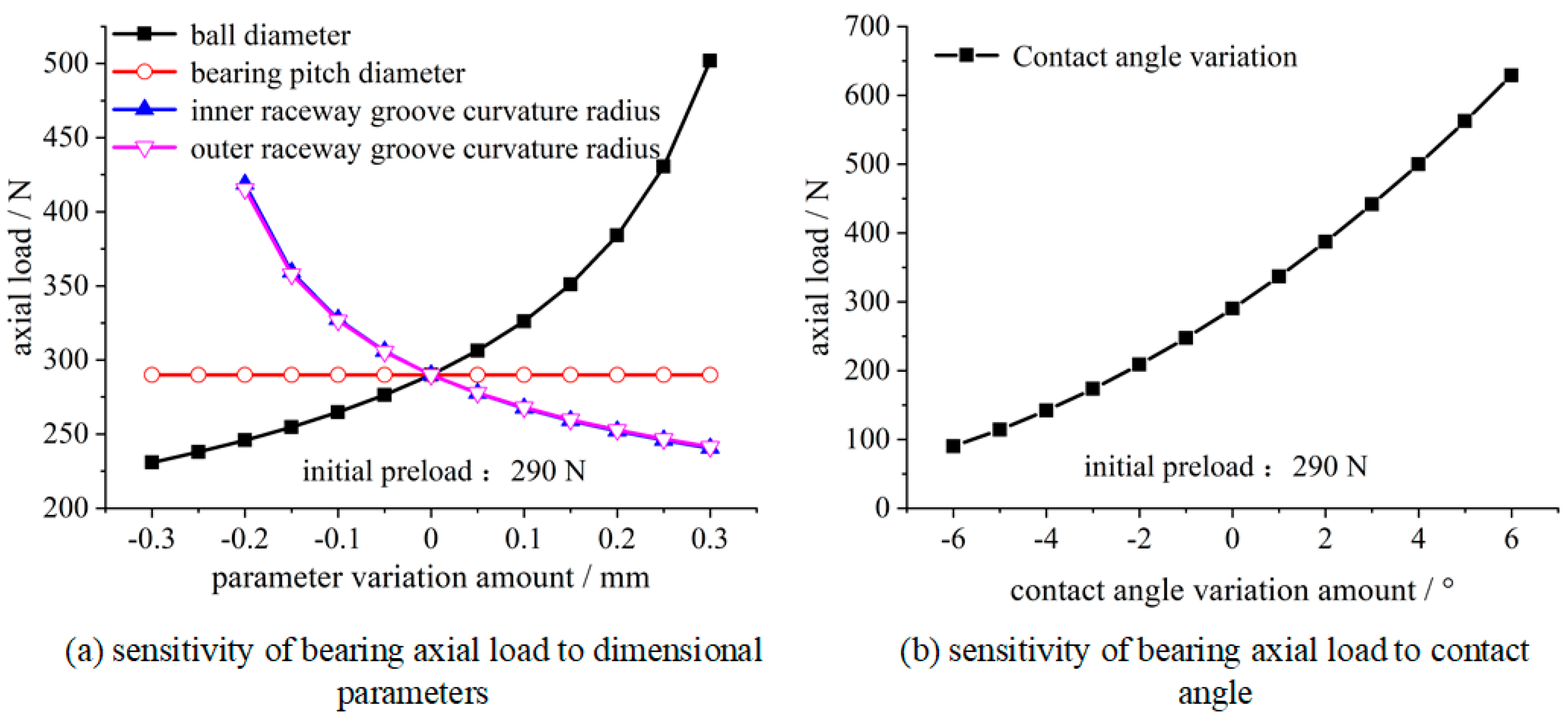
According to the modeling analysis of spindle stiffness in Section 2.2, the parameters required for spindle mechanics simulation mainly include: the number of balls, ball diameter, bearing pitch diameter, inner raceway groove curvature radius, outer raceway groove curvature radius, bearing contact angle, etc. Among them, the number of balls can generally be determined after the selection of bearing type, so its value does not need to be optimized in the process of parameter identification, while the bearing contact angle is the basic parameter for calculating the axial load–displacement coefficient of the bearing, which needs to be optimized. In order to both ensure the accuracy of the results and simplify the calculation, the parameters that have a greater influence on the calculation results can be optimized according to the sensitivity of the bearing mechanics calculation to each parameter. Therefore, based on the bearing mechanics model in Section 2.2, the influence of each parameter on the bearing axial load was analyzed (the bearing parameters are shown in Table 1), and the results are shown in Figure 8.

Table 1. The bearing parameters (NSK^®7014CTYNSULP4).

Parameters	Values
Number of balls	20
Ball diameter	11.906 mm
Bearing pitch diameter	90 mm
Inner raceway groove curvature radius	6.19112 mm
Outer raceway groove curvature radius	6.19112 mm
Initial contact angle of bearing	15°

Figure 8. Sensitivity analysis of bearing axial load to each parameter. (a) Sensitivity to ball diameter, pitch diameter, and raceway radii. (b) Sensitivity to dynamic contact angle variations.

As demonstrated in Figure 8a, changes in ball diameter and contact angle are positively correlated with changes in bearing axial load, whereas changes in inner raceway groove curvature radius and outer raceway groove curvature radius are negatively correlated. In particular, the variation in the above parameters has a large impact on the change in bearing axial load, so the ball diameter, contact angle, and inner/outer raceway groove curvature radius should be used as optimization parameters in the parameter identification process. In addition, it can also be found that the bearing axial load is almost unaffected by variations in the bearing pitch diameter. To provide a rigorous quantitative justification for excluding specific internal parameters from the optimization vector, a dimensionless sensitivity index S_i is introduced as follows:

$$S_i=\left|{\displaystyle \frac{\partial F_{ab}/F_{ab}}{\partial x_i/x_i}}\right|$$

(16)

where x_i denotes the specific internal geometric or material parameter of the bearing. Through numerical perturbation analysis, the calculated sensitivity indices for the ball diameter, initial contact angle, and inner/outer raceway curvature radii all exceed a critical engineering significance threshold (S_i > 0.5). Conversely, the sensitivity index for the bearing pitch diameter mathematically approaches zero (S_i = 8.6 × 10⁻⁶ ≪ 0.01). This definitive quantitative metric strictly confirms that variations in the pitch diameter yield negligible impact on the global axial force mapping, thereby justifying its exclusion from the optimization variables to minimize computational dimensionality and prevent algorithmic redundancy. Therefore, the corresponding optimization calculation is not required. The bearing contact angle is one of the key parameters in spindle stiffness identification, and it is strongly correlated with the rotational speed (as demonstrated in ref. [32]) and axial load (see Figure 8b), so the contact angle also needs to be used as an optimization parameter.

3.3. Optimized Objective Function

The parameter identification problem of spindle stiffness can be equated with the minimization problem. In order to make the optimized value of the spindle axial load–displacement data obtained by parameter identification accurately and truly reflect the variation law of the measured data and best fit the measured data, the mean squared difference between the optimized solved data and the measured data should be as small as possible. The optimized objective function is given as

$$f=\min \left(\sqrt{{\displaystyle \frac{1}{N}}{\displaystyle \sum _{i=1}^N{\left(F_{af}-F_a\right)}^2}}\right)$$

(17)

where N is the number of measured data points; F_af and F_a denote the optimized data and measured data of the axial load corresponding to the same axial displacement, respectively.

3.4. Constraints

Because several optimization techniques are used for parameter identification, the constraints that each optimization method specifies vary. In order to obtain the best parameter identification results, the constraints discussed in this study should only be viewed as proposed ranges, and their real ranges should be fine-tuned in accordance with the various optimization techniques. The specific constraints of each parameter are described as follows.

3.4.1. Ball Diameter Constraint

According to refs. [33,34], the range of values for optimizing the bearing ball diameter is described as follows:

$$K_{\min }{\displaystyle \frac{D_o-D_i}{2}}\le D\le K_{\max }{\displaystyle \frac{D_o-D_i}{2}}$$

(18)

where K represents the ball diameter coefficient. In general, K_min and K_max are 0.45 and 0.65, respectively. D_o is the bearing outer diameter. D_i denotes the bearing inner diameter.

3.4.2. Inner/Outer Raceway Groove Curvature Coefficient Constraint

The groove curvature coefficient f is often used to characterize the degree of proximity between the bearing ball and raceway for angular contact ball bearings, which satisfies the following relationship:

$$f_k={\displaystyle \frac{r_k}{D}}$$

(19)

where r denotes the bearing raceway groove curvature radius, and subscript k represents the ring scale i, o of the inner and outer ring, respectively. D is the bearing ball diameter.

According to refs. [33,34], for ball bearings, the range of values of f is described as follows:

$$0.505\le f_k\le 0.57$$

(20)

3.4.3. Contact Angle Constraint

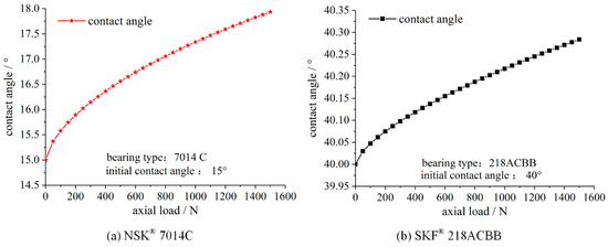
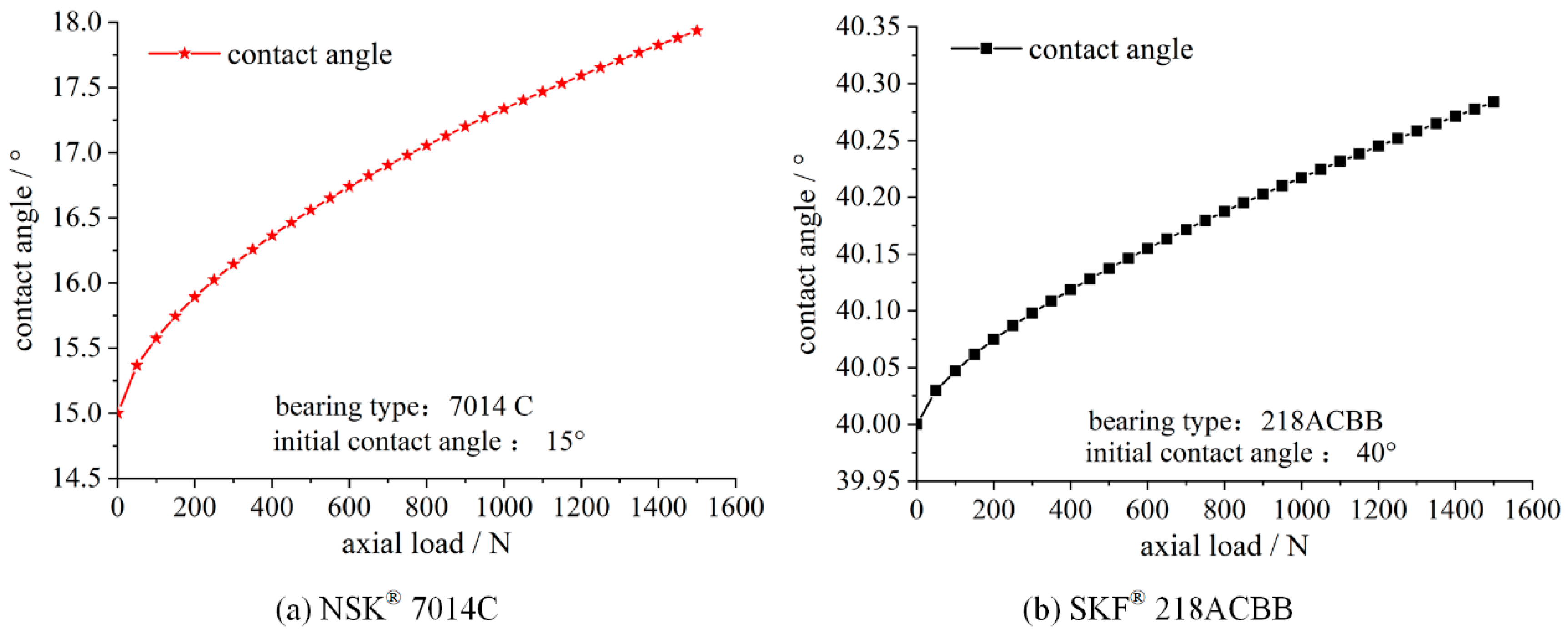
Due to the varying application requirements, each type of angular contact ball bearing has a distinct contact angle in its design, such as 15°, 18°, 25°, 30°, or 40°. In order to achieve the necessary bearing performance while using angular contact ball bearings, a particular preload is often applied. After preload is applied to the bearing, elastic deformation takes place in the contact region between the ball and the inner and outer raceways, causing a redistribution of loads inside the bearing, further resulting in a subsequent change in its contact angle. For a conventional angular contact ball bearing in a machine tool spindle configuration, the preload does not exceed 1500 N. As can be seen from Figure 9, the contact angle of the angular contact ball bearing typically changes by no more than 3° after the preload is applied. In addition, the initial contact angle of the bearing will typically have an error of ±2° after accounting for the effects of processing, manufacturing, and assembly flaws. As a result, it is advised to float the optimization range from the initial contact angle by around ±5°.

Figure 9. Bearing contact angle evolution under applied axial load: (a) 15° initial contact angle bearing (NSK 7014C); (b) 40° initial contact angle bearing (SKF 218ACBB).

3.4.4. Load–Displacement Coefficient Constraints in the Bearing Contact Area

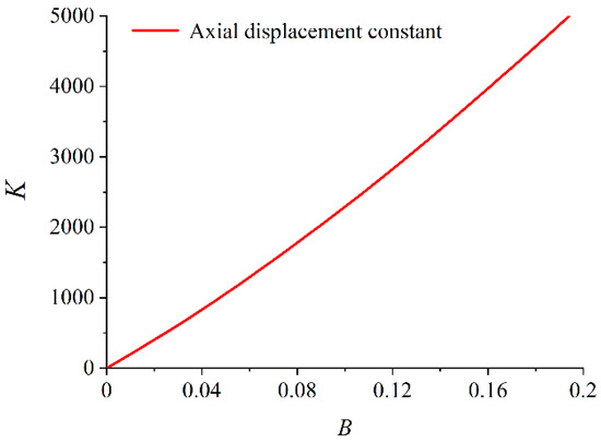
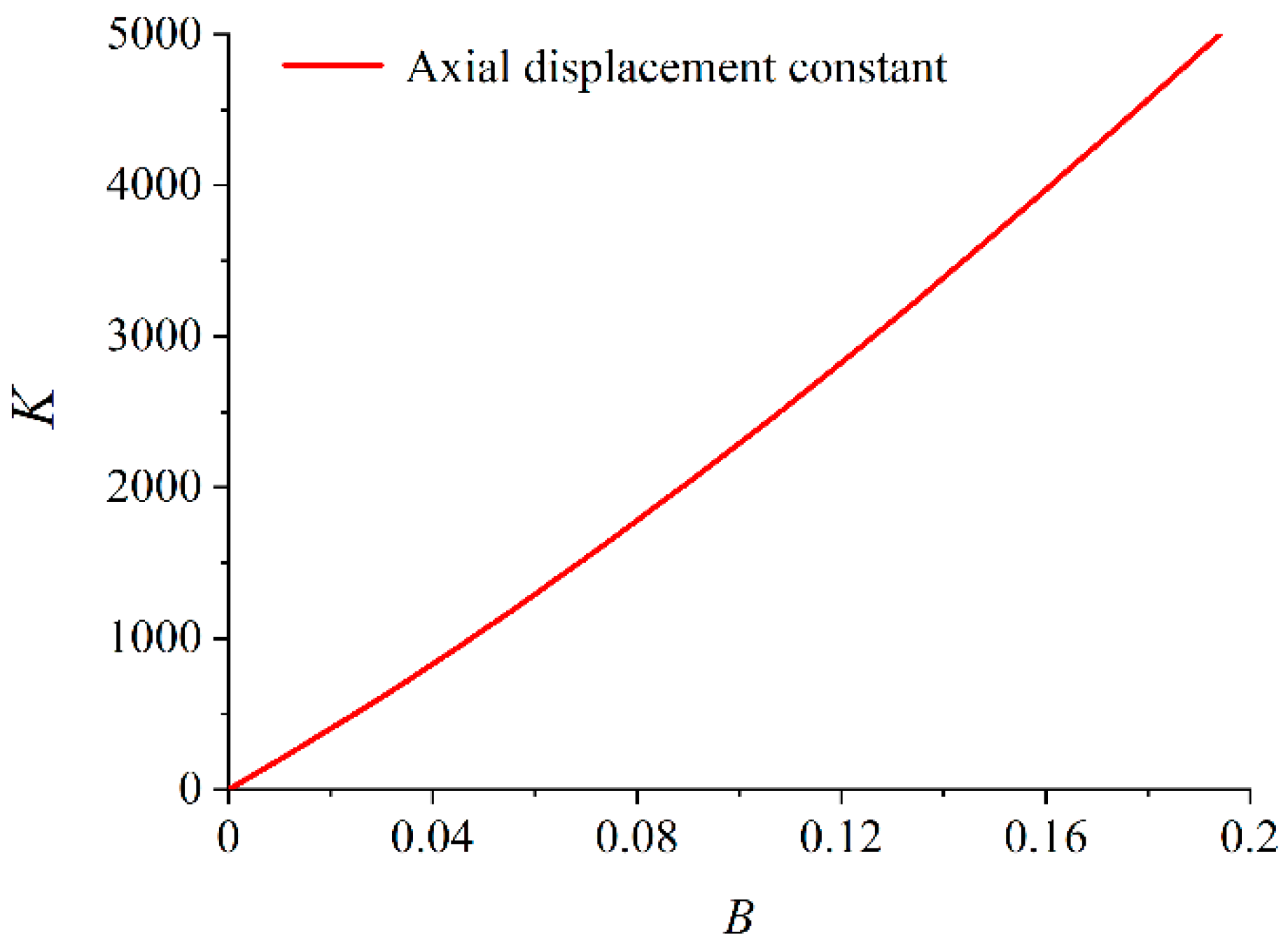
To determine the range of the bearing load–displacement coefficient K_n, the ball diameter and raceway groove curvature coefficients are first established based on Section 3.4.1 and Section 3.4.2. Next, the range of the axial displacement coefficient K is obtained from Figure 10 using the total bearing curvature B. Finally, the definitive range of K_n is calculated using Equation (21).

$$K_n={\displaystyle \frac{K{D}^{0.5}}{B^{1.5}}}$$

(21)

where D is the diameter of the bearing ball, and B denotes the total curvature, which can be calculated using Equations (19) and (22), respectively.

$$B=f_i+f_o-1$$

(22)

Figure 10. Analytical relationship between total bearing curvature B and axial displacement coefficient K [35].

3.5. Optimization Algorithm Selection

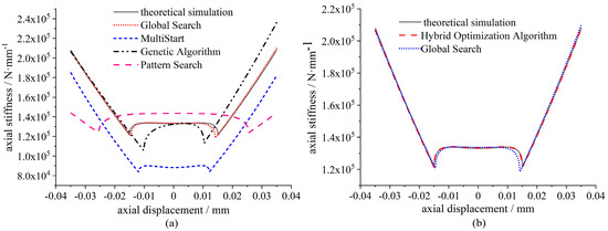
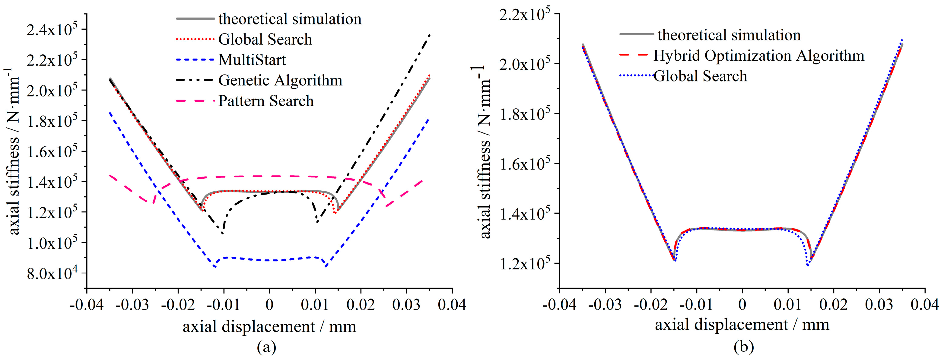
The parameter identification process is typically simplified into a curve-fitting or minimization problem. Optimization solutions are generally categorized as either local or global optima. However, local optima cannot guarantee the best parameter values across the entire function domain. Therefore, this study employs global optimization algorithms. Several mainstream global algorithms exist today. Common examples include MultiStart, genetic algorithms (GAs), Pattern Search, and Global Search. Based on the specific characteristics of parameter identification for spindle nonlinear stiffness, we selected several standard global optimization algorithms. To provide a rigorous mathematical benchmark for evaluating these algorithms prior to experimental deployment, a clean synthetic baseline—termed the “theoretical simulation” in Figure 11—is established. This baseline is explicitly generated via the forward calculation of the analytical spindle mechanics model (Equations (10)–(13)) described in Section 2.2, operating under ideal, noise-free conditions. By populating this forward mechanism model with the nominal geometric and material parameters of the NSK 7014C bearing (as listed in Table 1), we obtain a precise, physics-compliant load–displacement sequence. In this numerical validation approach, this sequence serves as the universally designated common input for all candidate optimization frameworks. The inverse identification performance of each algorithm is then quantitatively quantified by applying direct numerical differentiation to both the reconstructed and the baseline noise-free curves, thereby isolating the algorithmic accuracy from physical structural uncertainties. The computational results are presented in Figure 11a.

Figure 11. Convergence benchmark of optimization algorithms on synthetic data: (a) performance of single-stage routines (Global Search, MultiStart, GA, Pattern Search); (b) proposed two-stage hybrid optimization algorithm.

As shown in Figure 11a, the Global Search algorithm yields results closest to the theoretical simulations. While some computational error exists, it remains the smallest among all evaluated methods. Conversely, the MultiStart algorithm significantly underestimates the simulated values, resulting in the maximum computational error. The GA exhibits phase-dependent discrepancies. When both spindle bearings are loaded simultaneously, the GA values are slightly lower than the theoretical ones. However, once a single-end bearing is completely unloaded, the GA overestimates the forces. Additionally, the GA results are inconsistent between the spindle’s tension and compression phases, whereas the theoretical simulations are identical in both scenarios. The Pattern Search algorithm demonstrates the exact opposite trend to the GA. It slightly overestimates the theoretical results during simultaneous dual-bearing loading, but underestimates them following complete single-bearing unloading. Finally, we evaluated the axial displacement corresponding to the sudden change in spindle operational stiffness. With the exception of the Global Search and MultiStart algorithms, all other optimization methods demonstrate significant errors in capturing this specific metric compared to the theoretical simulations.

To improve the accuracy of parameter identification, we propose a hybrid optimization approach. This approach leverages the specific characteristics of different algorithms. Specifically, a second optimization algorithm is applied sequentially to refine the initial solution. First, the Global Search algorithm is utilized to optimize the spindle operational stiffness. This algorithm is notably insensitive to initial values. The resulting optimal solution is then used as the initial condition for the Pattern Search algorithm, which possesses strong robustness. This secondary optimization yields the final optimal parameters. As shown in Figure 11b, the error between the Global Search results and the theoretical simulation is 5.18%. In contrast, the hybrid optimization algorithm closely matches the simulation, significantly reducing the computational error to 0.67%. Evidently, this hybrid approach effectively combines the initial-value insensitivity of Global Search with the high robustness of Pattern Search. This synergy significantly enhances both the accuracy and robustness of parameter identification. Furthermore, using the first-stage optimization result as the initial condition for the second stage effectively improves the convergence of the algorithm.

To evaluate the algorithmic repeatability, convergence stability, and sensitivity to initial parameter guesses—thereby addressing the stochastic characteristics of heuristic mechanisms—a statistical robustness test was conducted. Specifically, a multistart Monte Carlo simulation comprising 100 independent optimization trials was executed using the synthetic baseline as the benchmark. In each trial, the initial guesses for the target vector (including ball diameter, contact angle, and raceway curvature coefficients) were randomly generated across their entire physical constraint spaces defined in Section 3.4. It is explicitly emphasized here that the primary theoretical objective of this Monte Carlo study is to rigorously evaluate the optimization landscape convexity and ensure that the two-stage hybrid algorithm reliably escapes local minima regardless of initial guesses, rather than to serve as a proof of noise immunity (which would inherently constitute a closed loop if tested solely against self-generated synthetic noise). To avoid circular logic and ensure methodological rigor, the algorithm’s capability to handle external uncertainties is not evaluated via idealized artificial white noise superimposed on the exact same model. Instead, robustness against non-ideal physical disturbances and system-level model mismatches is directly subjected to real-world empirical validation in Section 4. The statistical results demonstrate a high global convergence success rate, with the objective function uniformly minimizing to the same optimal basin. The variations among the identified structural parameters across the 100 randomized runs were found to be statistically negligible relative to their respective search dimensions, with the maximum relative deviation remaining well within a strict engineering tolerance (below 0.5%). This high level of consistency demonstrates that the proposed two-stage hybrid framework possesses high robustness against local minima entrapment and exhibits low sensitivity to initial parameter guesses, guaranteeing highly repeatable identification profiles under different initializations.

To further investigate the noise immunity of the proposed identification framework against varying measurement noise levels in a controlled numerical environment, additional sensitivity analyses were performed on the synthetic baseline. Zero-mean Gaussian white noise at relative intensities of 1%, 3%, and 5% (corresponding to signal-to-noise ratios (SNRs) of approximately 40 dB, 30 dB, and 26 dB, respectively) was superimposed onto the load–displacement target signals. The corrupted signals were sequentially processed using the SPA regularization filter and the two-stage hybrid optimization routine. As quantitatively summarized in Table 2, under the ideal noise-free baseline (0%), the maximum internal parameter identification error is only 0.35%, yielding a reconstructed stiffness curve RMSE of 0.67%. As the input noise level increases from 0% to 5%, the maximum identified parameter error increases gracefully to 4.12%, while the RMSE of the reconstructed stiffness curve remains bounded within 6.15%. This bounded, gradual error growth strictly confirms that the integration of regularized filtering with physics-constrained optimization provides robust noise immunity, effectively shielding the parameter identification process from high-level signal interference prior to real-world experimental deployment.

Table 2. Synthetic noise sensitivity analysis of the proposed identification framework.

Noise Level (%)/SNR	Input Displacement Noise RMS (μm)	Max Parameter Identification Error (%)	Reconstructed Stiffness Curve RMSE (%)
0% (Ideal Baseline)	0	0.35%	0.67%
1% (~40 dB)	0.38	0.85%	1.84%
3% (~30 dB)	1.14	2.15%	3.52%
5% (~26 dB)	1.90	4.12%	6.15%

From an engineering application perspective, since the static axial stiffness evaluation of machine tool spindles is inherently conducted as an offline baseline calibration or periodic maintenance procedure, the execution speed requirement is relatively secondary compared to feature extraction fidelity. To demonstrate the practical viability of the proposed hybrid optimization loop, its computational cost and convergence behavior were recorded on a standard engineering workstation (Intel Core i7, 16 GB RAM, MATLAB R2019a software platform). Under the initial preloads of 507 N and 862 N, the first-stage Global Search comprehensively explores the parameter space and establishes highly accurate initial boundaries within approximately 115 s. Guided by these optimal baselines, the second-stage Pattern Search rapidly achieves localized convergence in less than 40 iterations, consuming only about 18 s. The total execution time of the entire parameter identification framework averages 133 s. This rapid offline computing capacity strictly confirms that the methodology is fully suitable and highly efficient for practical machine tool engineering applications without requiring excessive high-performance computing resources.

4. Experimental Validation

4.1. Experimental Principle

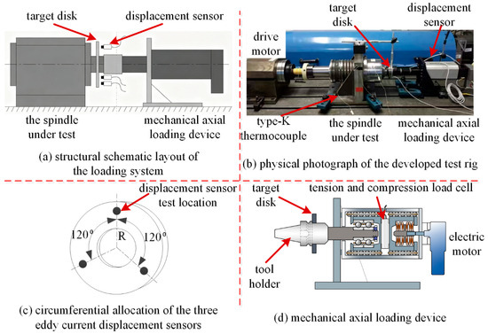
The overall experimental setup is illustrated in Figure 12a,b. To eliminate geometric errors, three sensors are allocated circumferentially as shown in Figure 12c. The detailed inner structure of the loader is depicted in Figure 12d. The experimental spindle is a mechanical shaft. It features a back-to-back arrangement with one front bearing and one rear bearing. The experimental setup utilizes a motorized spindle assembly. During the static stiffness tests in this study, the drive motor was kept unpowered (0 rpm), and static loads were directly applied to the spindle shaft using a precision mechanical loading device. K-type thermocouples measure the temperatures of key spindle components. A Yokogawa MX100^® data acquisition unit collects these temperature signals. The data is then automatically uploaded to a computer for recording. A custom-built testing device measures the axial stiffness of the spindle. During parameter adjustment, this device could act as a load and cause unnecessary interference. To prevent this, a custom quick-connector links the testing device to the spindle tool holder. Three high-precision eddy current displacement sensors are evenly distributed circumferentially (Figure 12). They synchronously measure the displacement of the target disk. These measurements are then averaged. This average accurately represents the axial displacement of the spindle end face along its centerline. Specifically, the displacement measurements are captured using eddy current displacement sensors (Model KD-2306-5SUM, KAMAN Company, Middletown, CT, USA) featuring a measurement range of 0–500 μm and a resolution accuracy up to 0.1 μm. Meanwhile, the axial load is applied and quantified via a high-precision force sensor (Model U3/5KN, Germany HBM, Darmstadt, Germany) with a measurement range of −5000 N to 5000 N, an accuracy grade of 0.5 N, and the capacity to withstand bidirectional tension and compression. Meanwhile, a custom mechanical loading device (Figure 12) automatically applies the axial load.

Figure 12. Experimental setup for spindle axial stiffness measurement: (a) schematic of mechanical loading system; (b) motorized spindle test bench; (c) circumferential 120° allocation of displacement sensors; (d) cross-section of axial loading unit.

The axial stiffness testing procedure includes the following steps: First, the motor is set to forward rotation. The loading device gradually applies a specific axial compressive force to the spindle. Next, the motor is set to reverse rotation. The loading device gradually reduces the compressive load to zero. It then applies an appropriate axial tensile force to the spindle. Finally, the motor returns to forward rotation. The loading device gradually reduces the tensile force to zero. During the test, an NI^®9215 data acquisition card automatically records the force and displacement signals in real time. The sampling frequency of the acquisition system is configured at 2048 Hz, yielding an overall dataset size of approximately 15,000 sampling points per experimental group for a complete loading–unloading cycle. When the spindle remains stationary at 0 rpm, the acquired signals consist purely of the quasi-static axial force and the corresponding multi-channel axial displacements under continuous load, establishing an expansive and high-resolution data volume to robustly evaluate the operational stiffness baseline without rotational dynamic interference. These signals are then uploaded to a computer for post-processing.

4.2. Results and Discussion

Table 1 shows the parameter settings for the experimental spindle bearings. We adjust the width difference between the inner and outer spacers of the spindle to set different preload levels. The experimental preloads are 507 N and 862 N. During the tests, the spindle speed is 0 rpm and the spindle temperature is 26 °C. Figure 13 displays the experimental results.

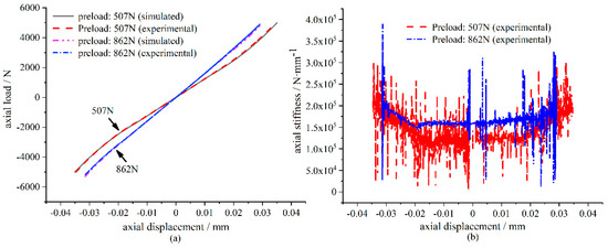
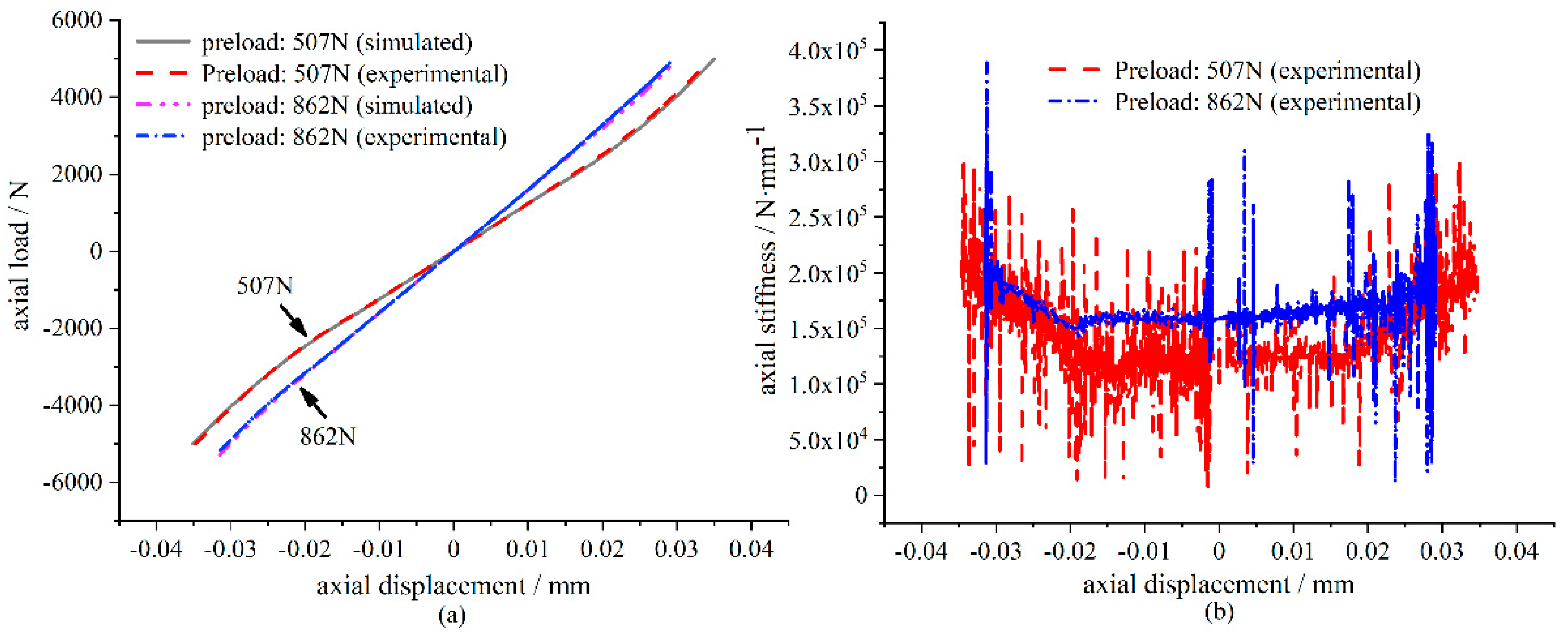
Figure 13. Spindle stiffness evaluated via direct differentiation under 507 N and 862 N initial preloads: (a) measured load–displacement curves; (b) derived stiffness profiles showing severe noise and lost nonlinear features.

To establish the baseline static stiffness, all experimental procedures were performed under stationary conditions (0 rpm), consistent with the operational setup described in Section 4.1. We use our custom-built testing device to apply axial tension and compression to the spindle. We simultaneously collect the corresponding axial displacement data. We then process this load–displacement data using the smoothness priors approach. Figure 13a compares the processed experimental data with the theoretical simulation curve. Figure 13a shows that the experimental and simulated results follow the same trend. The maximum errors are 1.7% (for a 507 N preload) and 2.1% (for an 862 N preload). Using the measured load–displacement data, we calculate the axial stiffness with the conventional method (Equation (23)). Figure 13b shows these results. This conventional method fails to capture the nonlinear characteristics of the spindle’s axial stiffness. However, Figure 13b does reveal one observation. The overall axial stiffness at an 862 N preload (1.6 × 10⁵ N·mm⁻¹) is slightly higher than at a 507 N preload (1.2 × 10⁵ N·mm⁻¹).

$$k_a={\displaystyle \frac{d{F}_{ab}}{d{\delta }_{ab}}}$$

(23)

Crucially, the raw experimental datasets displayed in Figure 13b inherently contain complex, high-level non-stationary measurement noise induced by target disk flatness errors, structural misalignments, and electromagnetic fluctuations. When subjected to conventional direct differentiation, this real-world noise undergoes severe derivative amplification, completely submerging the underlying stiffness characteristics and rendering traditional methods fully incapable of capturing any nonlinear trends. From a methodological perspective, validating the framework against real-world experimental data is fundamental to breaking the “circular logic” often encountered in purely synthetic numerical benchmarks. Synthetic noise profiles generated using predefined statistical distributions inherently mirror the foundational assumptions embedded within the mechanics model, creating a closed-loop validation that may mask identification vulnerabilities. In contrast, practical machine tool experimental signals contain complex, multi-source, non-Gaussian disturbances, along with unmodeled structural flexibilities (C_struct) and assembly-induced geometric runouts. Demonstrating that the proposed parameter identification framework can successfully filter these unmodeled shop-floor fluctuations and robustly reconstruct smooth, continuous stiffness profiles directly from raw, corrupted empirical signals provides an authentic, open-loop test of robustness. The fact that the proposed method can directly smooth out these significant fluctuations and accurately extract smooth, continuous stiffness profiles directly from these complex experimental signals provides definitive, side-by-side evidence of its exceptional noise immunity and practical robustness under different operational bounds (507 N and 862 N preloads).

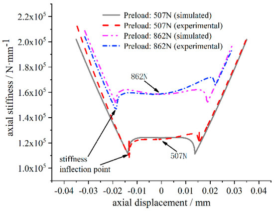
Based on the measured axial load–displacement data, we apply our proposed parameter identification method to determine the axial stiffness. Figure 14 shows the results. This method effectively captures the nonlinear characteristics of the spindle’s axial stiffness. The experimental results align well with the theoretical simulation trends. The maximum errors between these results are 12.3% (for a 507 N preload) and 11.6% (for an 862 N preload). A detailed physical evaluation of this approximately 12% discrepancy reveals that it stems from a fundamental divergence between the idealized system boundaries of the theoretical physics-driven model and the holistic structural realities of the experimental configuration, rather than algorithmic deficiencies. Primarily, while the theoretical formulation strictly isolates the localized Hertzian contact stiffness of the bearing pairs, the physical sensors inevitably record a composite macroscopic displacement at the spindle end face. This experimental boundary layer aggregates the axial compliance of the spindle shaft itself, the coupled stiffness of the tool holder assembly, and the structural contact compliances of the bearing housing and carrier fixtures. Furthermore, microscopic assembly and manufacturing realities introduce non-ideal boundaries; geometric form errors of the inner/outer spacers, micro-scale angular tilts during bearing installation, and joint interface friction collectively introduce localized compliance variations that are simplified in the theoretical model. From a metrological perspective, minute face runout (end-face jump) and residual geometric form deviations of the target disk introduce low-frequency deterministic disturbances into the displacement signals during continuous force loading. Despite these compounded engineering factors, restricting the identification error of a continuous, highly nonlinear stiffness profile within 12%—while successfully tracking the highly sensitive bearing unloading inflection points under complex, high-noise industrial shop floors—demonstrates remarkable robustness. This level of fidelity is entirely sufficient to satisfy rigorous industrial requirements for machine tool health monitoring, machining chatter prediction, and structural safety margin evaluation. Future work will focus on decoupling these macro-structural compliances to further isolate and optimize pure contact parameters.

Figure 14. Reconstructed continuous nonlinear axial stiffness profiles via the proposed method under 507 N and 862 N initial preloads, clearly identifying stiffness inflection points.

Figure 14 indicates that the overall axial stiffness at an 862 N preload is higher than at a 507 N preload. This is because the axial stiffness of a single bearing increases as the preload increases. The total stiffness of a position-preloaded spindle is the sum of the stiffness of the front and rear bearings. Therefore, a higher initial preload results in greater overall axial stiffness. Figure 14 also shows an abrupt change in axial stiffness under tensile and compressive loads. A higher preload corresponds to a larger absolute axial displacement at the point of this stiffness transition. This occurs because a higher preload increases the initial compression of the spindle. When the axial displacement fully offsets this initial compression, the stiffness transition occurs. At this point, the load-bearing state shifts from both bearings to a single bearing.

4.3. Quantitative Sensitivity Analysis of Unmodeled Structural Compliance

To rigorously address the ~12% discrepancy between the pure contact dynamic model and experimental measurements, an analytical sensitivity study quantifying the influence of shaft stiffness, housing compliance, and structural elasticities is established using the mechanics framework in Section 2.2.

By evaluating the difference between pure bearing stiffness K_b(F_a) and identified system stiffness K_id(F_a) from Equation (15), the relative identification error ε_K induced by omitting surrounding structural elasticities is analytically formulated as

$${\epsilon }_K={\displaystyle \frac{\left|K_b\left(F_a\right)-K_{id}\left(F_a\right)\right|}{K_b\left(F_a\right)}}={\displaystyle \frac{K_b\left(F_a\right)\cdot C_{struct}}{1+K_b\left(F_a\right)\cdot C_{struct}}}={\displaystyle \frac{K_b\left(F_a\right)}{K_b\left(F_a\right)+K_{struct}}}$$

(24)

Furthermore, the sensitivity coefficient S_c, defined as the first-order partial derivative of identified stiffness with respect to structural compliance variations, is derived as

$$S_c={\displaystyle \frac{\partial K_{id}}{\partial C_{struct}}}=-{\displaystyle \frac{K_b^2\left(F_a\right)}{{\left(1+K_b\left(F_a\right)\cdot C_{struct}\right)}^2}}$$

(25)

To evaluate this physical mechanism under actual testing conditions, numerical estimations were performed using the baseline equivalent structural stiffness of the shaft and housing assembly. Evaluating Equation (24) across the operating preload range yields theoretical identification error estimates (~12.2%) that align remarkably well with the experimentally observed verification errors of 12.3% (at 507 N preload) and 11.6% (at 862 N preload).

This quantitative analysis strictly proves that the ~12% error is not an artifact of numerical instability in parameter identification, but rather a mathematically deterministic consequence of unmodeled macro-structural elasticity (C_struct). Crucially, because C_struct acts as a linear background compliance in series with the contact zone, it uniformly scales the absolute magnitude without distorting the nonlinear profile or shifting critical bearing unloading inflection points.

5. Conclusions

This paper addresses the fundamental challenge of extracting nonlinear operational characteristics in machine tool spindle axial stiffness testing, which is heavily bottlenecked by experimental signal fluctuations and high-level measurement noise. A physics-driven parameter identification methodology is proposed, which successfully integrates the smoothness priors approach (SPA) for robust signal preprocessing with a mechanics-dependent hybrid optimization algorithm. The main conclusions and highlights of this study are summarized as follows:

(1)

High-Fidelity Signal Preprocessing: The implementation of the SPA-based algorithm effectively filters out high-frequency measurement noise from raw experimental data. By successfully preserving the true low-frequency displacement trends without phase distortion, this technique effectively improves the signal-to-noise ratio and provides a high-quality data foundation for overcoming the numerical divergence inherently caused by conventional differential operations.

(2)

Effective Feature Extraction and Noise Immunity: Numerical simulations (demonstrating < 4.12% parameter error under 5% synthetic noise) and experimental validations confirm that the proposed physics-driven approach successfully and accurately extracts the continuous evolution of spindle nonlinear axial stiffness profiles. In sharp contrast to conventional direct differentiation techniques that completely fail under noise interference, the proposed method clearly characterizes the distinct stiffness transition points and the nonlinear behavior during bearing unloading states.

(3)

Quantitative Mechanism of Structural Compliance Error: An analytical sensitivity formulation was integrated into the theoretical model to quantify the impact of unmodeled shaft and housing elasticities. The mathematical derivation strictly proves that the ~12% experimental verification error stems directly from the linear series compliance of surrounding structural components, while confirming that these macro-structural elasticities do not alter the nonlinear evolutionary trend or the critical bearing unloading inflection points.

In summary, this study provides a robust technical foundation for spindle performance evaluation and safety margin maintenance. Although the current validation focuses on the quasi-static baseline, the proposed physics-driven methodology possesses excellent structural extensibility, adapting directly to dynamic rotation and thermomechanical coupling by integrating advanced kinematic equations and thermal networks. Future endeavors will explicitly incorporate operational centrifugal forces, gyroscopic moments, and transient thermal expansion to achieve real-time dynamic stiffness tracking. Although the current offline computational cost of approximately 133 s is fully sufficient for standard workshop maintenance, future work will explicitly focus on compressing the algorithmic execution speed, reducing parameter searching dimensionality, and developing online real-time identification frameworks across diverse industrial operational environments.

References

- Cao, H.; Zhang, X.; Chen, X. The Concept and Progress of Intelligent Spindles: A Review. Int. J. Mach. Tools Manuf. 2017, 112, 21–52. [Google Scholar] [CrossRef] [Scilit]
- Dong, B.; Lei, C.; Liu, K.; Song, R.; Cui, P. Research on Dynamic Characteristics of Motorized Spindle Based on Comprehensive Stiffness of Angular Contact Ball Bearing. Mech. Sci. 2025, 16, 921–930. [Google Scholar] [CrossRef] [Scilit]
- Sun, F.; Jiang, Y.; Zhou, R.; Zhang, Q.; Xu, F.; Zhao, C.; Zhao, H.; Yang, W.; Li, B.; Bai, S. Research on the Consistency Evaluation of the Spindle Unit Stiffness Based on Comprehensive Weights. Machines 2024, 12, 426. [Google Scholar] [CrossRef] [Scilit]
- Wang, L.; Zhang, B.; Wu, J.; Zhao, Q.; Wang, J. Stiffness Modeling, Identification, and Measuring of a Rotating Spindle. Proc. Inst. Mech. Eng. Part C J. Mech. Eng. Sci. 2020, 234, 1239–1252. [Google Scholar] [CrossRef] [Scilit]
- Tai, C.-Y.; Altintas, Y. A Physics-Based Model-Data-Driven Method for Spindle Health Diagnosis, Part II: Dynamic Simulation and Validation. J. Manuf. Sci. Eng. 2024, 146, 081005. [Google Scholar] [CrossRef] [Scilit]
- Xue, R.; Zhang, P.; Huang, Z.; Wang, J. Digital Twin-Driven Fault Diagnosis for CNC Machine Tool. Int. J. Adv. Manuf. Technol. 2024, 131, 5457–5470. [Google Scholar] [CrossRef] [Scilit]
- Ma, S.; Leng, J.; Zheng, P.; Chen, Z.; Li, B.; Li, W.; Liu, Q.; Chen, X. A Digital Twin-Assisted Deep Transfer Learning Method towards Intelligent Thermal Error Modeling of Electric Spindles. J. Intell. Manuf. 2025, 36, 1659–1688. [Google Scholar] [CrossRef] [Scilit]
- Tai, C.-Y.; Altintas, Y. A hybrid physics and data-driven model for spindle fault detection. CIRP Ann. 2023, 72, 353–356. [Google Scholar] [CrossRef] [Scilit]
- Tai, C.-Y.; Altintas, Y. A Physics-Based Model-Data-Driven Method for Spindle Health Diagnosis, Part III: Model Training and Fault Detection. J. Manuf. Sci. Eng. 2024, 146, 081006. [Google Scholar] [CrossRef] [Scilit]
- Liu, X.; Zhao, C.; Xu, F.; Zhao, W.; Jin, J.; Man, R.; Liu, J.; Sun, F. Numerical Study on Raceway Wear of Angular Contact Ball Bearings Considering Curvature Radius Variation. Machines 2026, 14, 664. [Google Scholar] [CrossRef] [Scilit]
- Cun, H.; Yuan, S.; Cui, G.; Li, J. Static Stiffness Analysis and Experimental Study of Spindle System of Machine Tool. Mach. Tool Hydraul. 2015, 43, 32–36. [Google Scholar]
- Cui, F.; Li, Y.; Yu, J.; Tang, A.; Li, P.; Han, L. Simulation and Experimental Study on the Static Stiffness of High Speed Motorized Spindle. J. Mech. Strength 2017, 39, 971–975. [Google Scholar]
- Bardac, D.; Dogariu, C. Finite Element Analysis for Static Behaviour of the CNC Turning Machine Spindle. In Proceedings of the 2014 3rd International Conference on Applied Mechanics and Materials (ICAMM 2014); Trans Tech Publications: Shenzhen, China, 2014; Volume 555, pp. 555–560. [Google Scholar]
- Huang, M.; Zhang, C. Test and Analysis for Static Stiffness of High Speed Motorized Spindle. Mach. Tool Hydraul. 2018, 46, 106–109. [Google Scholar]
- Liu, G.; Hong, J.; Wu, W.; Sun, Y. Investigation on the Influence of Interference Fit on the Static and Dynamic Characteristics of Spindle System. Int. J. Adv. Manuf. Technol. 2018, 99, 1953–1966. [Google Scholar] [CrossRef] [Scilit]
- Li, J.; Zhu, Y.; Yan, K.; Yan, X.; Liu, Y.; Hong, J. Research on the Axial Stiffness Softening and Hardening Characteristics of Machine Tool Spindle System. Int. J. Adv. Manuf. Technol. 2018, 99, 951–963. [Google Scholar] [CrossRef] [Scilit]
- Li, J.; Tian, J.; Su, H.; Bian, C.X.; Xia, Y.F.; Liu, T.Y.; Chen, X.J.; Wang, P.; Li, D.Z. Study on the 2D Equivalent Nonlinear Dynamics Simulation Model Related to High Speed Precision Bearing and Spindle. Precis. Eng. 2024, 91, 358–371. [Google Scholar] [CrossRef] [Scilit]
- Wei, Y.; Xu, F. Nonlinear Dynamic Analysis of Spindle System Considering Thermal-Solid Coupling. Nonlinear Dyn. 2025, 113, 6049–6073. [Google Scholar]
- Fang, B.; Zhang, J.; Hong, J.; Yan, K. Research on the Nonlinear Stiffness Characteristics of Double-Row Angular Contact Ball Bearings under Different Working Conditions. Lubricants 2023, 11, 44. [Google Scholar] [CrossRef] [Scilit]
- Li, J.; Wang, Q.; Sun, X.; Qu, J.; Qiu, A.; Kang, W.; Ma, S. Research on the Effect of Spindle Speed on the Softening and Hardening Characteristics of the Axial Operating Stiffness of Machine Tool Spindle. Lubricants 2022, 10, 132. [Google Scholar] [CrossRef] [Scilit]
- Li, T.; Kolar, P.; Li, X.-Y.; Wu, J. Research Development of Preload Technology on Angular Contact Ball Bearing of High Speed Spindle: A Review. Int. J. Precis. Eng. Manuf. 2020, 21, 1163–1185. [Google Scholar]
- Kessels, B.M.; Fey, R.H.B.; van de Wouw, N. Real-time parameter updating for nonlinear digital twins using inverse mapping models and transient-based features. Nonlinear Dyn. 2023, 111, 18889–18910. [Google Scholar] [CrossRef] [Scilit]
- Kessels, B.M.; Fey, R.H.B.; van de Wouw, N. Uncertainty quantification in real-time parameter updating for digital twins using Bayesian inverse mapping models. Nonlinear Dyn. 2024, 116, 1515–1532. [Google Scholar] [CrossRef] [Scilit]
- Dong, X.; Sun, F.; Li, Y.; Yang, G.; Liu, L.; Xu, F.; Zhao, H.; Zhang, Q.; Zhou, R. Stiffness Optimization of Electric Spindle Performance Based on Multi-Layer Perceptron Integrated Bayesian. Sci. Rep. 2025, 15, 1. [Google Scholar] [CrossRef] [Scilit] [PubMed]
- Qiao, G.; Xu, J.; Zhang, Y.; Zhao, C. An Identification Method of Dynamic Stiffness and Damping for the Spindle Bearing System of a CNC Lathe. Mech. Syst. Signal Process. 2024, 222, 111808. [Google Scholar] [CrossRef] [Scilit]
- Li, J.; Bian, C.; Su, H.; Jing, T.; Xia, Y.; Liu, T.; Jia, C.; Chen, X.; Wang, P.; Li, D. Study on the Structural Design of a High-Precision Spindle Based on an Efficient 2D Equivalent Thermo-Mechanical Finite Element Model. Precis. Eng. 2026. [Google Scholar] [CrossRef] [Scilit]
- Zhang, X.; Ma, Z.; Jiang, Y. Fault Diagnosis of High-Speed Motorized Spindles Based on Lumped Parameter Model and Enhanced Transfer Learning. Struct. Health Monit. 2025, 24, 1841–1858. [Google Scholar] [CrossRef] [Scilit]
- Tarvainen, M.P.; Ranta-Aho, P.O.; Karjalainen, P.A. An Advanced Detrending Method with Application to HRV Analysis. IEEE Trans. Biomed. Eng. 2002, 49, 172–175. [Google Scholar] [CrossRef] [Scilit] [PubMed]
- Yu, Z.; Fang, X.; Zhang, W.; Huang, J.; Ding, K. Passive Acoustic Signal Trend Items Removal Based on SPA. J. Detect. Control 2015, 37, 34–36+41. [Google Scholar]
- Günther, C.; Hofmeister, B.; Hübler, C.; Jonscher, C.; Ragnitz, J.; Schubert, J.; Steinbach, M.C. Damage Location in Mechanical Structures by Multi-Objective Pattern Search. Optim. Eng. 2025, 26, 1365–1405. [Google Scholar]
- Zhou, W.; Zhong, L.; Kang, W.; Xu, Y.; Luan, C.; Fu, J. Modal Parameter Identification of Electric Spindles Based on Covariance-Driven Stochastic Subspace. Machines 2024, 12, 774. [Google Scholar] [CrossRef] [Scilit]
- Antoine, J.-F.; Abba, G.; Molinari, A. A New Proposal for Explicit Angle Calculation in Angular Contact Ball Bearing. J. Mech. Des. 2006, 128, 468–478. [Google Scholar] [CrossRef] [Scilit]
- Deng, S.; Jia, Q.; Xue, J. Rolling Bearing Design Principle; Standards Press of China: Beijing, China, 2014. [Google Scholar]
- Yu, D. Research on Mechanical Characteristics and Multi Objective Optimization Design of RV Reducer Main Bearing. Master’s Thesis, Xi’an Jiaotong University, Xi’an, China, 2017. [Google Scholar]
- Harris, T.; Kotzalas, M. Rolling Bearing Analysis: Essential Concepts of Bearing Technology, 5th ed.; CRC Press: New York, NY, USA, 2007. [Google Scholar]
Disclaimer/Publisher’s Note: The statements, opinions and data contained in all publications are solely those of the individual author(s) and contributor(s) and not of MDPI and/or the editor(s). MDPI and/or the editor(s) disclaim responsibility for any injury to people or property resulting from any ideas, methods, instructions or products referred to in the content. |
© 2026 by the authors. Licensee MDPI, Basel, Switzerland. This article is an open access article distributed under the terms and conditions of the Creative Commons Attribution (CC BY) license.