Kinematic Modelling and Co-Simulation-Based Posture Control of a Solid Backfilling Support Robot for Coal Mining

Abstract

The solid backfilling support robot is key equipment for intelligent backfill mining, but its dual-top-beam structure, multiple closed-loop linkages and hydraulically actuated compaction mechanism make posture representation, inverse actuator mapping and control execution strongly coupled. This study develops a unified kinematic modelling and mechanical–hydraulic-control co-simulation workflow for a ZC5160/30/50 solid backfilling hydraulic support. Closed-loop vector equations are derived for the main support mechanism, rear top-beam mechanism and compaction mechanism, and the mappings among actuator strokes, posture angles and key node positions are established. An engineering posture-index system is constructed for roof contact, support adjustment and backfilling–compaction operation. Forward and inverse kinematic modules are implemented in MATLAB/Simulink and checked using an ADAMS virtual prototype. Representative workspace sampling further shows that all 15 inverse–forward verification cases converge and satisfy actuator stroke constraints, while the residual Jacobians remain full rank with maximum condition numbers of 9.135–9.950. An ADAMS-AMESim-MATLAB/Simulink co-simulation platform is then used to evaluate actuator tracking and PID-based posture-control feasibility. The numerical comparison shows good consistency for the main rigid-body posture indices, whereas conveyor-related relative-position indices show larger deviations because the suspended conveyor motion is affected by gravity in the virtual prototype. Under two target posture cases, the top-beam and compaction-mechanism angle deviations remain within ±0.3°, and the height deviation is below 5 mm. The proposed workflow provides a simulation basis for posture perception, actuator planning and control-system design of solid backfilling support robots; the reported results should be interpreted as model-level numerical consistency and co-simulation feasibility rather than physical prototype accuracy.

1. Introduction

Solid backfill mining technology has demonstrated significant advantages in surface subsidence control, ecological environmental governance and the resource utilization of mine solid waste [1,2]. Under the current context of energy-industry transformation, the improvement of coal productivity relies heavily on the synergistic development of digitalization, intelligence and greening, a trend that is driving mining equipment toward intelligent, unmanned and robotic operation [3,4]. Research on mining robot crowds has further emphasized that unmanned working faces depend on the coordinated operation of robotized equipment, including shearers, hydraulic supports and scraper conveyors [5]. In particular, the robotization of coal-mine equipment has become a critical driving force for the high-quality development of the coal industry [6]. From the perspective of smart-mine system engineering, intelligent equipment, sensing, control and coordinated operation are key technical foundations for unmanned mining systems [7]. As core equipment of intelligent backfill systems, solid backfilling support robots must simultaneously provide roof support, maintain backfilling space and assist the compaction of filling materials. Previous studies on backfilling hydraulic supports have evaluated operating performance using hybrid machine learning models and investigated structural reformation and design methods [8,9]. These studies highlight the engineering importance of backfilling supports, but they mainly focus on performance evaluation or structural design rather than inverse kinematic mapping and posture-control co-simulation of a dual-top-beam, compaction-coupled support robot.

Regarding the posture perception and posture solution of hydraulic supports, extensive research has been conducted. Zeng et al. established a single-support posture perception model based on multi-rod dual-drive and a group posture perception model based on spatial multi-line cooperative determination [10]. Pang et al. achieved numerical solutions for support posture and height by establishing position-relation equations for the hinge points of main structural components and using the Newton–Raphson method [11]. Beyond posture measurement, position and posture detection and control systems for hydraulic supports have also been investigated, showing that posture solution and actuator control are essential for autonomous support adjustment [12]. Zhang et al. proposed a method for detecting the relative position and posture of hydraulic supports based on the principle of determining a plane with three non-collinear points [13]. In addition, scholars have explored using support-condition acquisition, depth vision and virtual simulation methods to obtain top-beam posture, support height and full-pose information of hydraulic supports [14,15,16]. However, solid backfilling support robots feature dual top beams, multiple closed-loop linkage groups, conveyor-related spatial constraints and a compaction mechanism. These structural characteristics lead to highly nonlinear kinematic coupling among mechanisms, making conventional hydraulic-support posture models difficult to apply directly.

In the integration of modelling theory and simulation, forward and inverse kinematic solutions provide the computational basis for posture perception and control-system design. Yan investigated key technologies in hydraulic-support virtual monitoring systems [17], Zhang achieved spatial coordinate transformation through D-H matrix analysis [18], and Lin and Miao derived analytical expressions for the motion posture coordinates of chock-shield hydraulic powered supports [19]. Lu et al. analyzed the inverse kinematics of hydraulic supports [20], and Meng et al. constructed a mechanical–electrical–hydraulic co-simulation model based on ADAMS, AMESim and Simulink to analyze hydraulic-support posture adjustment [21]. More recent work has shown that mechanical–hydraulic co-simulation and valve-controlled cylinder analysis are important for evaluating hydraulic-support execution mechanisms, because hydraulic flow limitation, valve delay and actuator response can strongly affect the final control performance [22,23]. Distributed cooperative control has also been investigated for hydraulic-support robot groups during frame-moving operations [24]. Nevertheless, most existing studies still focus on conventional hydraulic supports, group movement coordination or isolated hydraulic-control problems. For solid backfilling support robots with dual top beams, a compaction mechanism and conveyor-related spatial constraints, an integrated workflow linking closed-loop mechanism kinematics, engineering posture indices, inverse actuator mapping and mechanical–hydraulic-control co-simulation remains insufficient.

Studies on intelligent solid backfilling support robots and mechanism-interference characterization have reported key technologies and autonomous demodulation strategies for solid backfilling equipment [25,26]. However, few studies have integrated dual-top-beam closed-loop kinematics, compaction-mechanism coupling, engineering posture indices and mechanical–hydraulic-control co-simulation into a unified modelling workflow for a solid backfilling support robot.

To further clarify the research gap, representative studies related to backfilling supports, hydraulic-support posture modelling, inverse kinematics and hydraulic-control simulation are compared in Table 1. Existing studies have provided important foundations for support-pose perception, kinematic modelling, hydraulic actuator control and intelligent backfilling equipment. However, the integration of dual-top-beam closed-loop kinematics, compaction-mechanism coupling, engineering posture indices and mechanical–hydraulic–control co-simulation remains insufficient for solid backfilling support robots.

Table 1. Comparison of representative studies related to hydraulic-support posture modelling and control.

Reference	Research Focus	Backfilling/Compaction Mechanism	Co-Simulation	Difference from This Study
Pang et al. [11], Lu et al. [20]	Posture and inverse kinematic solution of hydraulic supports	No	No	Conventional supports; no dual-top-beam or compaction-mechanism coupling
Zhang et al. [12,13]	Position/posture detection and control of hydraulic supports	No	Partly related	Focuses on pose detection and control rather than unified inverse mapping and co-simulation
Wang et al. [16]	Full-pose measurement and virtual simulation of solid filling support	Partly related	No	Does not establish a complete mechanical–hydraulic-control co-simulation workflow
Meng et al. [21]	Mechanical–electrical–hydraulic coordinated simulation	No	Yes	Co-simulation for conventional support posture adjustment
Zeng et al. [22], Hou et al. [23]	Hydraulic actuator/feedforward/positioning control	No	Hydraulic-control focused	Focuses on local hydraulic execution rather than whole-machine posture modelling
Zhang et al. [25] and this study	Intelligent solid backfilling support robot	Yes	This study: Yes	Existing work provides equipment background; this study links closed-loop kinematics, posture indices and co-simulation

Addressing this gap, this study develops a unified modelling and co-simulation workflow for a solid backfilling support robot with dual top beams, multiple closed-loop linkages and a compaction mechanism. The contribution is organized at three levels. First, closed-loop vector equations are established for the main support mechanism, rear top-beam mechanism and compaction mechanism, thereby describing the geometric coupling among actuator strokes, posture angles and key node positions. Second, an engineering posture-index system is constructed for roof-contact, support-adjustment and backfilling–compaction operations. Third, the kinematic model is connected with an ADAMS-AMESim-MATLAB/Simulink co-simulation platform to evaluate inverse actuator mapping, hydraulic execution and PID-based posture-control feasibility. The verification in this paper is based on virtual-prototype and co-simulation results; therefore, the results are interpreted as model-level numerical consistency and control-process feasibility rather than physical prototype validation.

2. Structural Feature Analysis and Kinematic Model Construction of Solid Backfill Support Robot

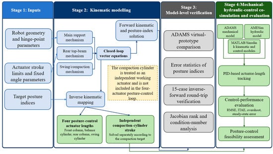
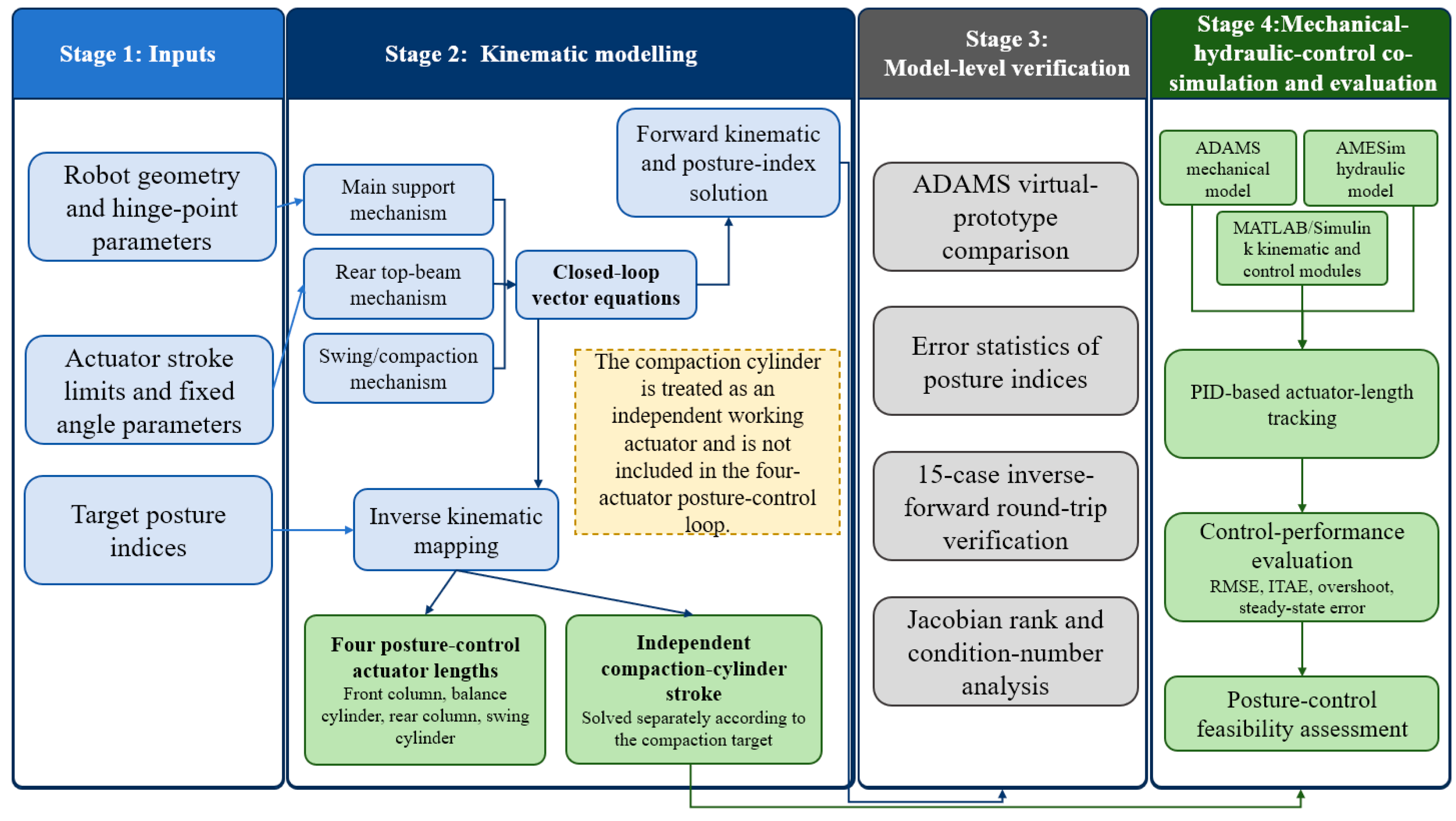
Before the detailed kinematic derivation, the overall workflow of the proposed modelling and co-simulation method is shown in Figure 1. The workflow starts from robot geometry, actuator stroke limits and target posture indices, and then establishes closed-loop vector equations for the main support mechanism, rear top-beam mechanism and swing/compaction mechanism. The forward and inverse kinematic modules are verified through ADAMS virtual-prototype comparison, inverse–forward sampling and Jacobian conditioning analysis. Finally, the inverse actuator commands are introduced into the ADAMS–AMESim–MATLAB/Simulink co-simulation platform to evaluate hydraulic execution and posture-control feasibility.

Figure 1. Overall workflow of the proposed kinematic modelling and mechanical–hydraulic-control co-simulation method.

2.1. Analysis of Structural Features and the Degree of Freedom

2.1.1. Structural Features

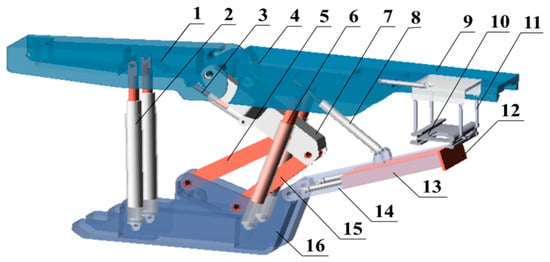
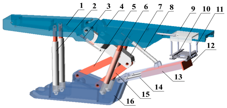
The backfill support robot was developed based on the existing solid backfill hydraulic support and the backfill scraper conveyor as the machinery foundation [24], mainly consisting of the base, the four-linkage mechanism, the front and the rear columns, and the compaction mechanism. To be specific, the front of the support was similar to the shielded support; the compaction mechanism was composed of the swing angle cylinder and the compaction cylinder; the compaction cylinder was hinged to the base; the swing angle cylinder was hinged to the rear top beam on the one end and to the compaction beam on the other end to achieve the regulation of the compaction angle, as shown in Figure 2.

Figure 2. Structural composition of the developed intelligent solid backfill support robot: 1. Front top beam. 2. Front column. 3. Balance cylinder. 4. Rear top beam. 5. Front connecting rod. 6. Rear column. 7. Upper connecting rod. 8. Swing angle cylinder. 9. Rear hinge beam. 10. Sliding rail of the backfill conveyor. 11. Chute lifting ring. 12. Baffle. 13. Compaction mechanism. 14. Pendulum beam. 15. Rear connecting rod. 16. Base.

2.1.2. DoF Calculations

The backfill support robot is a complex series-parallel mechanism. According to the Grubler–Kutzbach formula, the number of degrees of freedom (DoF) can be calculated as:

$$F=s\times \left(n-m-1\right)+{\displaystyle \sum _{i=1}^m{f}_i-v-q}$$

(1)

where s denotes the order of the mechanism, λ denotes the common constraint number (s = 6 − λ), n denotes the number of components, m denotes the number of the moving pairs of the mechanism, f denotes the relative DoF of the i-th movement pair, v denotes the virtual constraint number, and q denotes the local DoF.

After removing the compaction mechanism, as shown in Figure 2, the total number of components in the mechanism was n = 12, the number of moving pairs was m = 15, and three common constraints existed (in the two-dimensional plane λ = 3). According to the order of the mechanism (s = 6 − λ), s = 3, i.e., the mechanism is a third-order mechanism (v = 0 and q = 0). For the two-column protective hydraulic support, the DoF of the main body can be calculated as:

$$F=3\times \left(12-15-1\right)+15=3$$

(2)

The remaining numbers remained unchanged after adding the compaction mechanism, n = 16, m = 20. The DoF of the backfill support robot can be calculated as:

$$F=3\times \left(16-20-1\right)+20=5$$

(3)

According to the DoF analysis, the backfill support robot can be simplified as a planar linkage mechanism with five DoFs (F = 5) for kinematic analysis.

According to the DoF analysis, the complete planar mechanism of the backfilling support robot has five DoFs for kinematic analysis. It should be emphasized that these five DoFs describe the mobility of the complete mechanism, rather than the number of inputs used in the main posture-control loop. In the posture-control model developed in this paper, the front column, balance cylinder, rear column and swing cylinder form a four-actuator posture-adjustment subsystem. These four actuators determine the main posture variables of the dual top beams and the swing angle of the compaction mechanism. The remaining actuated motion corresponds to the extension of the compaction cylinder, which is treated as an independent working actuator for adjusting the terminal position or stroke of the compaction plate during backfilling operation. Therefore, the inverse kinematic posture-control module solves the strokes of the four posture-control actuators, whereas the compaction-cylinder stroke is solved or controlled separately according to the compaction target. The geometric constants, fixed angle parameters and actuator stroke constraints used in the kinematic calculation are summarized in Appendix A.

2.2. Establishment of the Kinematic Equation of the Developed Backfill Support Robot

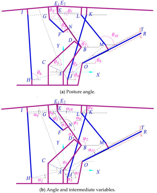
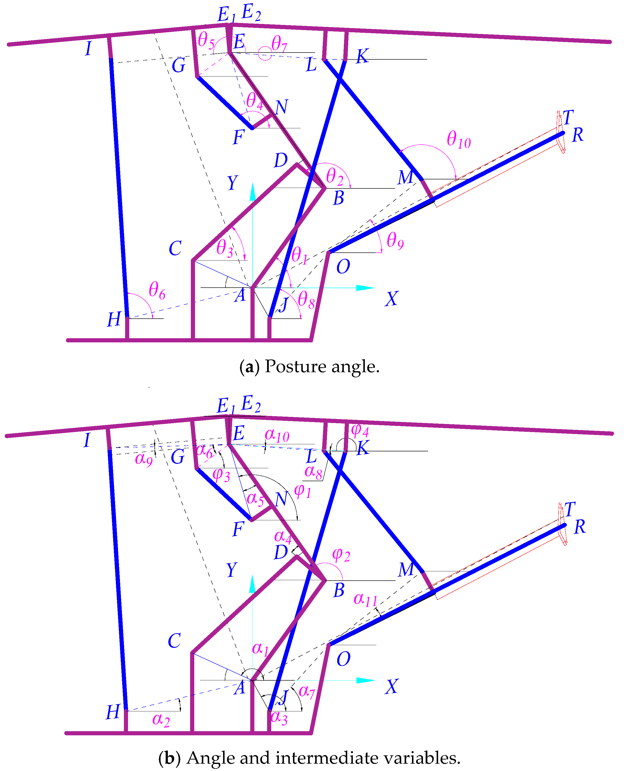
The kinematics of the developed solid backfill support robot were analyzed using the closed-loop vector method. Taking the ZC5160/30/50 solid backfill hydraulic support as an example, the mechanisms with correlated motion states were first analyzed, and the relative variables in the kinematic analysis of the main mechanism are shown in Figure 3.

Figure 3. Posture variables of the mechanical body of the developed solid backfill support robot.

In Figure 3, letters A to P denote the hinge points of various mechanisms, which were regarded as the rotational joints in kinematic analysis; the other points, including N, P, Q, R, T, E₁, and E₂, were points on the mechanism. By assuming that θ₁~θ₁₀ denote the posture variables to be determined, φ₁~φ₄ denote the intermediate variables, α₁~α₈ denote the known angle constant parameters, starting from the positive direction of x-axis, and setting the counterclockwise rotation as positive, φ₁ and φ₂ can be transformed as the expression of θ₂, φ₃ can be transformed as the expression of θ₅ and φ₄ can be transformed as the expression of θ₇:

$$\left\{\begin{array}{l}{\phi }_1={\phi }_2-{\alpha }_5\\ {\phi }_2={\theta }_2-{\alpha }_4\\ {\phi }_3={\theta }_5+{\alpha }_6-\pi \\ {\phi }_4={\theta }_7+{\alpha }_8-\pi \end{array}\right.$$

(4)

The front part of the backfill support robot was composed of three closed loops: ABDC, EFG, and ABEIH.

$$\left\{\begin{array}{l}\overrightarrow{AB}+\overrightarrow{BD}=\overrightarrow{AC}+\overrightarrow{CD}\\ \overrightarrow{FE}=\overrightarrow{FG}+\overrightarrow{GE}\\ \overrightarrow{HI}=\overrightarrow{HA}+\overrightarrow{AB}+\overrightarrow{BE}+\overrightarrow{EI}\end{array}\right.$$

(5)

After determining the posture of the front part of the support, the posture of the rear top beam of the support can be determined by supplementing the ABFKJ closed loop:

$$\overrightarrow{JK}=\overrightarrow{JA}+\overrightarrow{AB}+\overrightarrow{BE}+\overrightarrow{EK}$$

(6)

After the posture of both front and rear top beams of the support was determined, the compaction angle of the compaction mechanism can be determined by supplementing the JOMLK closed loop:

$$\overrightarrow{JA}+\overrightarrow{AB}+\overrightarrow{BE}+\overrightarrow{EL}=\overrightarrow{JK}+\overrightarrow{KL}$$

(7)

Using the complex vector method, the following expressions can be derived:

$$\left\{\begin{array}{l}{L}_{AB}{e}^{i{\theta }_1}+L_{BD}{e}^{i{\theta }_2}=L_{AC}{e}^{i{\alpha }_1}+L_{CD}{e}^{i{\theta }_3}\\ L_{FG}{e}^{i{\theta }_4}+L_{GE}{e}^{i{\phi }_3}=L_{FE}{e}^{i{\phi }_1}\\ L_{HI}{e}^{i{\theta }_6}=L_{HA}{e}^{i{\alpha }_2}+L_{AB}{e}^{i{\theta }_1}+L_{BE}{e}^{i{\phi }_2}+L_{EI}{e}^{i{\theta }_5}\end{array}\right.$$

(8)

$$L_{JK}{e}^{i{\theta }_8}+L_{JA}{e}^{i{\alpha }_3}=L_{AB}{e}^{i{\theta }_1}+L_{BE}{e}^{i{\phi }_2}+L_{EK}{e}^{i{\theta }_7}$$

(9)

$$L_{JO}{e}^{i{\alpha }_7}+L_{OM}{e}^{i{\theta }_9}+L_{ML}{e}^{i{\theta }_{10}}=L_{JK}{e}^{i{\theta }_8}+L_{KL}{e}^{i{\phi }_4}$$

(10)

in which L_AB, L_AC, L_BD, L_CD, L_BE, L_FG, L_FN, L_EG, L_HI, L_JK, L_ML, L_AJ, L_JO, L_OR, L_EK, L_EL, and L_EE1 represent the corresponding geometric sizes. Points Q and P are auxiliary equivalent points introduced on the front and rear top beams, respectively. In the kinematic derivation, they are used to express the generalized motion of representative top-beam points in the closed-loop vector formulation. When the force-mapping relationship is discussed, they can be interpreted as equivalent application points of the resultant roof-contact load. They are not measured variables, statistically sampled points or independent control inputs in the posture-control model. Point T denotes any point on the surface of the compaction mechanism. Point P represents the position of the resultant force of the external load on the rear top beam. Point T denotes any point on the surface of the compaction mechanism.

According to Euler’s formula, both imaginary and real parts of the above formulas were separated and simplified, and the following expressions can be derived:

$$\left\{\begin{array}{l}{L}_{AB}\cos \left({\theta }_1\right)+L_{BD}\cos \left({\theta }_2\right)=L_{AC}\cos \left({\alpha }_1\right)+L_{CD}\cos \left({\theta }_3\right)\\ L_{AB}\sin \left({\theta }_1\right)+L_{BD}\sin \left({\theta }_2\right)=L_{AC}\sin \left({\alpha }_1\right)+L_{CD}\sin \left({\theta }_3\right)\\ L_{FG}\cos \left({\theta }_4\right)+L_{GE}\cos \left({\phi }_3\right)=L_{FE}\cos \left({\phi }_1\right)\\ L_{FG}\sin \left({\theta }_4\right)+L_{GE}\sin \left({\phi }_3\right)=L_{FE}\sin \left({\phi }_1\right)\\ L_{HI}\cos \left({\theta }_6\right)=L_{HA}\cos \left({\alpha }_2\right)+L_{AB}\cos \left({\theta }_1\right)+L_{BE}\cos \left({\phi }_2\right)+L_{EI}\cos \left({\theta }_5\right)\\ L_{HI}\sin \left({\theta }_6\right)=L_{HA}\sin \left({\alpha }_2\right)+L_{AB}\sin \left({\theta }_1\right)+L_{BE}\sin \left({\phi }_2\right)+L_{EI}\sin \left({\theta }_5\right)\end{array}\right.$$

(11)

where θ₁, θ₂, θ₃, θ₄, θ₅ and θ₆ denote the posture variables to be determined; L_HI and L_FG denote the motion variables. Equation (11) implies that the height of the four-linkage mechanism of the inclination angle of the front top beam can be determined by the front column and the balance oil cylinder.

Similarly, the posture equations of the rear top beam can be determined as:

$$\left\{\begin{array}{l}{L}_{JK}\cos \left({\theta }_8\right)=L_{JA}\cos \left({\alpha }_3\right)+L_{AB}\cos \left({\theta }_1\right)+L_{BE}\cos \left({\phi }_2\right)+L_{EK}\cos \left({\theta }_7\right)\\ L_{JK}\sin \left({\theta }_8\right)=L_{JA}\sin \left({\alpha }_3\right)+L_{AB}\sin \left({\theta }_1\right)+L_{BE}\sin \left({\phi }_2\right)+L_{EK}\sin \left({\theta }_7\right)\end{array}\right.$$

(12)

where θ₇ and θ₈ denote the posture variables to be determined; L_JK denotes the motion variable. Accordingly, the posture of the rear top beam can be obtained by solving θ₁ and θ₂.

Similarly, the posture equations of the rear top beam can be determined as:

$$\left\{\begin{array}{l}{L}_{JO}\cos \left({\alpha }_7\right)+L_{OM}\cos \left({\theta }_9\right)+L_{ML}\cos \left({\theta }_{10}\right)=L_{JK}\cos \left({\theta }_8\right)+L_{KL}\cos \left({\phi }_4\right)\\ L_{JO}\sin \left({\alpha }_7\right)+L_{OM}\sin \left({\theta }_9\right)+L_{ML}\sin \left({\theta }_{10}\right)=L_{JK}\sin \left({\theta }_8\right)+L_{KL}\sin \left({\phi }_4\right)\end{array}\right.$$

(13)

where θ₉ and θ₁₀ denote the posture variables to be determined; L_ML denotes the motion variable. Accordingly, the posture of the rear top beam can be obtained by solving θ₇ and θ₈.

3. Kinematic Equation of the Backfill Support Robot

3.1. Forward Kinematic Solution to the Mechanism

3.1.1. Mapping Relations of the Velocities of the Front Column and the Balance Cylinder and the Velocity of the Front Top Beam

According to the structural features of the backfill support robot, the front and rear top beams can be regarded as two parallel moving platforms [13]. Therefore, a mapping relation exists between the front top beam/the front column and the input velocity of the balance cylinder.

According to the kinematic equation as shown in Equation (8), by taking the derivative concerning time, the following expressions can be derived:

$$\left\{\begin{array}{l}{L}_{AB}{\dot{\theta }}_1\sin \left({\theta }_1\right)+L_{BD}{\dot{\theta }}_2\sin \left({\theta }_2\right)-L_{CD}{\dot{\theta }}_3\sin \left({\theta }_3\right)=0\\ L_{AB}{\dot{\theta }}_1\cos \left({\theta }_1\right)+L_{BD}{\dot{\theta }}_2\cos \left({\theta }_2\right)-L_{CD}{\dot{\theta }}_3\cos \left({\theta }_3\right)=0\\ L_{FE}{\dot{\theta }}_2\sin \left({\theta }_2-{\alpha }_4-{\alpha }_5\right)-L_{FG}{\dot{\theta }}_4\sin \left({\theta }_4\right)-L_{GE}{\dot{\theta }}_5\sin \left({\theta }_5+{\alpha }_6-\pi \right)={\dot{L}}_{FG}\cos \left({\theta }_4\right)\\ L_{FE}{\dot{\theta }}_2\cos \left({\theta }_2-{\alpha }_4-{\alpha }_5\right)-L_{FG}{\dot{\theta }}_4\cos \left({\theta }_4\right)-L_{GE}{\dot{\theta }}_5\cos \left({\theta }_5+{\alpha }_6-\pi \right)={\dot{L}}_{FG}\sin \left({\theta }_4\right)\\ L_{AB}{\dot{\theta }}_1\sin \left({\theta }_1\right)+L_{BE}{\dot{\theta }}_2\sin \left({\theta }_2-{\alpha }_4\right)+L_{EI}{\dot{\theta }}_5\sin \left({\theta }_5\right)-L_{HI}{\dot{\theta }}_6\sin \left({\theta }_6\right)={\dot{L}}_{HI}\cos \left({\theta }_6\right)\\ L_{AB}{\dot{\theta }}_1\cos \left({\theta }_1\right)+L_{BE}{\dot{\theta }}_2\cos \left({\theta }_2-{\alpha }_4\right)+L_{EI}{\dot{\theta }}_5\cos \left({\theta }_5\right)-L_{HI}{\dot{\theta }}_6\cos \left({\theta }_6\right)={\dot{L}}_{HI}\sin \left({\theta }_6\right)\end{array}\right.$$

(14)

In matrix form, Equation (14) can be rewritten as:

$$A{\left[{\dot{\theta }}_1 {\dot{\theta }}_2 {\dot{\theta }}_3 {\dot{\theta }}_4 {\dot{\theta }}_5 {\dot{\theta }}_6\right]}^T=C{\left[{\dot{L}}_{FG} {\dot{L}}_{HI}\right]}^T$$

(15)

where

$$A=\left[\begin{array}{llllll}{L}_{AB}\sin \left({\theta }_1\right)& L_{BD}\sin \left({\theta }_2\right)& - L_{CD}\sin \left({\theta }_3\right)& 0& 0& 0\\ L_{AB}\cos \left({\theta }_1\right)& L_{BD}\cos \left({\theta }_2\right)& -L_{CD}\cos \left({\theta }_3\right)& 0& 0& 0\\ 0& L_{FE}\sin \left({\phi }_1\right)& 0& -L_{FG}\sin \left({\theta }_4\right)& -L_{GE}\sin \left({\phi }_3\right)& 0\\ 0& L_{FE}\cos \left({\phi }_1\right)& 0& -L_{FG}\cos \left({\theta }_4\right)& -L_{GE}\cos \left({\phi }_3\right)& 0\\ L_{AB}\sin \left({\theta }_1\right)& L_{BE}\sin \left({\phi }_2\right)& 0& 0& L_{EI}\sin \left({\theta }_5\right)& -L_{HI}\sin \left({\theta }_6\right)\\ L_{AB}\cos \left({\theta }_1\right)& L_{BE}\cos \left({\phi }_2\right)& 0& 0& L_{EI}\cos \left({\theta }_5\right)& -L_{HI}\cos \left({\theta }_6\right)\end{array}\right]$$

(16)

$$C=\left[\begin{array}{ll}0& 0\\ 0& 0\\ \cos \left({\theta }_4\right)& 0\\ \sin \left({\theta }_4\right)& 0\\ 0& \cos \left({\theta }_6\right)\\ 0& \sin \left({\theta }_6\right)\end{array}\right]$$

(17)

The matrix A was invertible, and the mapping relation between the posture of the front top beam/the front column and the stroke of the balance cylinder can be written as:

$${\left[{\dot{\theta }}_1 {\dot{\theta }}_2 {\dot{\theta }}_3 {\dot{\theta }}_4 {\dot{\theta }}_5 {\dot{\theta }}_6\right]}^T=A^{-1}C{\left[{\dot{L}}_{FG} {\dot{L}}_{HI}\right]}^T$$

(18)

where A⁻¹C denotes the velocity Jacobian matrix of the six posture angles (θ₁~θ₆). The mapping relation among the velocities of the front column, the balance oil cylinder and the top beam can be established.

To express the generalized motion of a representative point on the front top beam, an auxiliary point Q(x, y) is selected on the front top beam, and the closed-loop vector ABEE₁Q is introduced. In the subsequent force-mapping interpretation, Q may be regarded as the equivalent application point of the resultant roof-contact load on the front top beam. However, Q is not used as an additional posture-control target in this paper.

$$L_{AQ}{e}^{i{\theta }_Q}=L_{AB}{e}^{i{\theta }_1}+L_{BE}{e}^{i{\phi }_2}+L_{E{E}_1}{e}^{i\left({\theta }_5+{\alpha }_9-{\displaystyle \frac{\pi }{2}}\right)}+L_{E_{1}Q}{e}^{i\left({\theta }_5+{\alpha }_9\right)}$$

(19)

Through separation, Equation (19) can be rewritten as:

$$\left\{\begin{array}{l}{X}_Q=L_{AB}\cos \left({\theta }_1\right)+L_{BE}\cos \left({\phi }_2\right)+L_{E{E}_1}\cos \left({\theta }_5+{\alpha }_9-{\displaystyle \frac{\pi }{2}}\right)+L_{E_{1}Q}\cos \left({\theta }_5+{\alpha }_9\right)\\ Y_Q=L_{AB}\sin \left({\theta }_1\right)+L_{BE}\sin \left({\phi }_2\right)+L_{E{E}_1}\sin \left({\theta }_5+{\alpha }_9-{\displaystyle \frac{\pi }{2}}\right)+L_{E_{1}Q}\sin \left({\theta }_5+{\alpha }_9\right)\end{array}\right.$$

(20)

By taking the derivative with respect to time, the following expression can be obtained:

$$\left\{\begin{array}{l}{\dot{X}}_Q=-L_{AB}{\dot{\theta }}_1\sin \left({\theta }_1\right)-L_{BE}{\dot{\theta }}_2\sin \left({\phi }_2\right)-\left[L_{E{E}_1}\sin \left({\theta }_5+{\alpha }_9-{\displaystyle \frac{\pi }{2}}\right)+L_{E_{1}Q}\sin \left({\theta }_5+{\alpha }_9\right)\right]{\dot{\theta }}_5\\ {\dot{Y}}_Q=L_{AB}{\dot{\theta }}_1\cos \left({\theta }_1\right)+L_{BE}{\dot{\theta }}_2\cos \left({\phi }_2\right)+\left[L_{E{E}_1}\cos \left({\theta }_5+{\alpha }_9-{\displaystyle \frac{\pi }{2}}\right)+L_{E_{1}Q}\cos \left({\theta }_5+{\alpha }_9\right)\right]{\dot{\theta }}_5\end{array}\right.$$

(21)

By adding the generalized velocity component θ₅ into the matrix, we get:

$${\left[{\dot{X}}_Q {\dot{Y}}_Q {\dot{\theta }}_5\right]}^T=B{\left[{\dot{\theta }}_1 {\dot{\theta }}_2 {\dot{\theta }}_3 {\dot{\theta }}_4 {\dot{\theta }}_5 {\dot{\theta }}_6\right]}^T$$

(22)

where

$$B=\left[\begin{array}{llllll}-L_{AB}\sin \left({\theta }_1\right)& -L_{BE}\sin \left({\phi }_2\right)& 0& 0& -L_{E{E}_1}\sin \left({\theta }_5+{\alpha }_9-{\displaystyle \frac{\pi }{2}}\right)-L_{E_{1}Q}\sin \left({\theta }_5+{\alpha }_9\right)& 0\\ L_{AB}\cos \left({\theta }_1\right)& L_{BE}\cos \left({\phi }_2\right)& 0& 0& L_{E{E}_1}\cos \left({\theta }_5+{\alpha }_9-{\displaystyle \frac{\pi }{2}}\right)+L_{E_{1}Q}\cos \left({\theta }_5+{\alpha }_9\right)& 0\\ 0& 0& 0 & 0& 1& 0\end{array}\right]$$

(23)

Through a combination, the following expression can be derived:

$${\left[{\dot{X}}_Q {\dot{Y}}_Q {\dot{\theta }}_5\right]}^T=J{\left[{\dot{L}}_{FG} {\dot{L}}_{HI}\right]}^T$$

(24)

where J = BA⁻¹C denotes the velocity Jacobian matrix. The generalized velocities of the front column and the balance jack ${\left[{\dot{L}}_{FG} {\dot{L}}_{HI}\right]}^T$ can be mapped to the generalized velocity of the front top beam ${\left[{\dot{X}}_Q {\dot{Y}}_Q {\dot{\theta }}_5\right]}^T$.

3.1.2. Theoretical Force-Mapping Relation of the Front Top-Beam Mechanism

Based on the velocity Jacobian derived above, a theoretical force-mapping relationship can be established between the actuator forces of the front column and balance cylinder and the generalized force acting on the front top beam. This relationship is introduced to keep the kinematic model compatible with subsequent mechanical analysis, rather than to perform quantitative roof-load identification in this study. The corresponding force Jacobian can be written as:

$${\left[F_1 F_3\right]}^T=J_F{\left[F_{Qx} F_{Qy} M_Q\right]}^T$$

(25)

At static equilibrium, according to the principle of virtual work (d’Alembert), the work done by the driving force of the support equaled the work done by the applied external load:

$$\left[{\dot{L}}_{FG} {\dot{L}}_{HI}\right]{\left[F_1 F_3\right]}^T=\left[{\dot{X}}_Q {\dot{Y}}_Q {\dot{\theta }}_5\right]{\left[F_{Qx} F_{Qy} M_Q\right]}^T$$

(26)

By combining Equations (25) and (26), the following expression can be derived:

$$\left[{\dot{L}}_{FG} {\dot{L}}_{HI}\right]J_F{\left[F_{Qx} F_{Qy} M_Q\right]}^T=\left[{\dot{X}}_Q {\dot{Y}}_Q {\dot{\theta }}_5\right]{\left[F_{Qx} F_{Qy} M_Q\right]}^T$$

(27)

Considering the arbitrariness of the generalized force ${\left[{\mathrm{F}}_{{\mathrm{Q}}_{\mathrm{x}}}{\mathrm{F}}_{{\mathrm{Q}}_{\mathrm{y}}}{\mathrm{M}}_{\mathrm{Q}}\right]}^{\mathrm{T}}$

$$\left[{\dot{L}}_{FG} {\dot{L}}_{HI}\right]J_F=\left[{\dot{X}}_Q {\dot{Y}}_Q {\dot{\theta }}_5\right]$$

(28)

Meanwhile, after transposition, the following expression can be written as:

$$J_F^T{\left[{\dot{L}}_{FG} {\dot{L}}_{HI}\right]}^T={\left[{\dot{X}}_Q {\dot{Y}}_Q {\dot{\theta }}_5\right]}^T=J{\left[{\dot{L}}_{FG} {\dot{L}}_{HI}\right]}^T$$

(29)

Considering the arbitrariness of [L_FG L_HI]:

$$J_F^T=J or J_F=J^T$$

(30)

where J^T denotes the force Jacobian that maps the actuator forces of the front column and balance cylinder to the generalized force of the front top beam. In this study, this equation is retained as a theoretical force-mapping interface between the closed-loop kinematic model and actuator force analysis. It should not be interpreted as a calibrated working-resistance calculation or an external-load identification method.

Because J^T is a 3 × 2 matrix rather than a square matrix, the generalized external load cannot be uniquely recovered by directly inverting J^T. Therefore, quantitative working-resistance design would require additional information, including calibrated roof-contact load distribution, contact-region parameters and structural dynamic conditions. These issues are beyond the scope of the present study, which focuses on posture solution, inverse actuator mapping and mechanical–hydraulic-control co-simulation.

3.1.3. Velocity and Theoretical Force-Mapping Relation of the Rear Top-Beam Mechanism

Given the front-top-beam posture, the values of θ₁ and θ₂ can be determined. The velocity and force-mapping relationship of the rear top-beam mechanism can then be formulated as follows:

$$\left\{\begin{array}{l}-L_{EK}{\dot{\theta }}_7\sin \left({\theta }_7\right)+L_{JK}{\dot{\theta }}_8\sin \left({\theta }_8\right)={\dot{L}}_{JK}\cos \left({\theta }_8\right)\\ L_{EK}{\dot{\theta }}_7\cos \left({\theta }_7\right)-L_{JK}{\dot{\theta }}_8\cos \left({\theta }_8\right)={\dot{L}}_{JK}\sin \left({\theta }_8\right)\end{array}\right.$$

(31)

Similarly, the following expression can be derived:

$$A_1{\left[{\dot{\theta }}_7 {\dot{\theta }}_8\right]}^T=C_1{\dot{L}}_{JK}$$

(32)

in which

$$A_1=\left[\begin{array}{ll}-L_{EK}\sin \left({\theta }_7\right)& L_{JK}\sin \left({\theta }_8\right)\\ L_{EK}\cos \left({\theta }_7\right)& -L_{JK}\cos \left({\theta }_8\right)\end{array}\right]$$

(33)

$$C_1=\left[\begin{array}{l}\cos \left({\theta }_8\right)\\ \sin \left({\theta }_8\right)\end{array}\right]$$

(34)

On account of the reversibility of A₁, the mapping relation between the pose of the rear top beam of the support and the stroke of the rear column can be written as:

$${\left[{\dot{\theta }}_7 {\dot{\theta }}_8\right]}^T=A_1^{-1}{C}_1{\dot{L}}_{JK}$$

(35)

Similarly, an auxiliary point P(x, y) is selected on the rear top beam to express the generalized motion of a representative rear top-beam point through the closed-loop vector ABEE₂P. In the force-mapping interpretation, P can be regarded as the equivalent application point of the resultant roof-contact load on the rear top beam. It is not treated as a separately measured, optimized or controlled variable in the present posture-solution model.

$$L_{AP}{e}^{i{\theta }_P}=L_{AB}{e}^{i{\theta }_1}+L_{BE}{e}^{i{\phi }_2}+L_{E{E}_2}{e}^{i\left({\theta }_7+{\alpha }_{10}-{\displaystyle \frac{\pi }{2}}\right)}+L_{E_{2}P}{e}^{i\left({\theta }_7+{\alpha }_{10}\right)}$$

(36)

Through separation, the following expression can be derived:

$$\left\{\begin{array}{l}{X}_P=L_{AP}\cos \left({\theta }_P\right)=L_{AB}\cos \left({\theta }_1\right)+L_{BE}\cos \left({\phi }_2\right)+L_{E{E}_2}\cos \left({\theta }_7+{\alpha }_{10}-{\displaystyle \frac{\pi }{2}}\right)+L_{E_{2}P}\cos \left({\theta }_7+{\alpha }_{10}\right)\\ Y_P=L_{AP}\sin \left({\theta }_P\right)=L_{AB}\sin \left({\theta }_1\right)+L_{BE}\sin \left({\phi }_2\right)+L_{E{E}_2}\sin \left({\theta }_7+{\alpha }_{10}-{\displaystyle \frac{\pi }{2}}\right)+L_{E_{2}P}\sin \left({\theta }_7+{\alpha }_{10}\right)\end{array}\right.$$

(37)

By taking the derivative with respect to time, the following expression can be derived:

$$\left\{\begin{array}{l}{\dot{X}}_P=-\left[L_{E{E}_2}\sin \left({\theta }_7+{\alpha }_{10}-{\displaystyle \frac{\pi }{2}}\right)+L_{E_{2}P}\sin \left({\theta }_7+{\alpha }_{10}\right)\right]{\dot{\theta }}_7\\ {\dot{Y}}_P=\left[L_{E{E}_2}\cos \left({\theta }_7+{\alpha }_{10}-{\displaystyle \frac{\pi }{2}}\right)+L_{E_{2}P}\cos \left({\theta }_7+{\alpha }_{10}\right)\right]{\dot{\theta }}_7\end{array}\right.$$

(38)

By adding the generalized velocity component θ₇ into the matrix:

$${\left[{\dot{X}}_P {\dot{Y}}_P {\dot{\theta }}_7\right]}^T=B_1{\left[{\dot{\theta }}_7 {\dot{\theta }}_8\right]}^T$$

(39)

where

$$B_1=\left[\begin{array}{ll}-\left[L_{E{E}_2}\sin \left({\theta }_7+{\alpha }_{10}-{\displaystyle \frac{\pi }{2}}\right)+L_{E_{2}P}\sin \left({\theta }_7+{\alpha }_{10}\right)\right]& 0\\ \left[L_{E{E}_2}\cos \left({\theta }_7+{\alpha }_{10}-{\displaystyle \frac{\pi }{2}}\right)+L_{E_{2}P}\cos \left({\theta }_7+{\alpha }_{10}\right)\right]& 0\\ 1& 0\end{array}\right]$$

(40)

Through a combination, the following expression can be obtained:

$${\left[{\dot{X}}_P {\dot{Y}}_P {\dot{\theta }}_7\right]}^T=J_1{\dot{L}}_{JK}$$

(41)

where J₁ = B₁A₁⁻¹C₁ denotes the velocity Jacobian matrix. The generalized velocity of the rear column is mapped to the generalized velocity of the rear top beam.

Similarly, the following expression can be derived:

$$F_2=J_{F_1}{\left[F_{Px} F_{Py} M_P\right]}^T$$

(42)

where ${\mathrm{J}}_{{\mathrm{F}}_1}={{\mathrm{J}}_1}^{\mathrm{T}}$ denote the force Jacobian matrix.

3.1.4. Mapping Relation Between the Velocity of the Swing Cylinder and the Velocity of the Posture Angle of the Compaction Mechanism

By moving to the other side of the equation and taking the first-order derivative with respect to time, the following expression can be obtained:

$$\left\{\begin{array}{l}-L_{OM}{\dot{\theta }}_9\sin \left({\theta }_9\right)-L_{ML}{\dot{\theta }}_{10}\sin \left({\theta }_{10}\right)=-{\dot{L}}_{ML}\cos \left({\theta }_{10}\right)\\ L_{OM}{\dot{\theta }}_9\cos \left({\theta }_9\right)+L_{ML}{\dot{\theta }}_{10}\cos \left({\theta }_{10}\right)=-{\dot{L}}_{ML}\sin \left({\theta }_{10}\right)\end{array}\right.$$

(43)

In matrix form, Equation (43) can be rewritten as:

$$A_2{\left[{\dot{\theta }}_9 {\dot{\theta }}_{10}\right]}^T=C_2 {\dot{L}}_{ML}$$

(44)

where

$$A_2=\left[\begin{array}{ll}-L_{OM}\sin \left({\theta }_9\right)& -L_{ML}\sin \left({\theta }_{10}\right)\\ L_{OM}\cos \left({\theta }_9\right)& L_{ML}\cos \left({\theta }_{10}\right)\end{array}\right]$$

(45)

$$C_2=\left[\begin{array}{l}-\cos \left({\theta }_{10}\right)\\ -\sin \left({\theta }_{10}\right)\end{array}\right]$$

(46)

Based on the above analysis results, A₂ was reversible. Accordingly, the mapping relation between the posture angle of the compaction mechanism and the stroke of the swing cylinder can be written as:

$${\left[{\dot{\theta }}_9 {\dot{\theta }}_{10}\right]}^T=A_2^{-1}{C}_2{\dot{L}}_{ML}$$

(47)

The solution to the displacement of the swing cylinder based on the posture angle according to Equation (47) can be achieved, laying the foundation for realizing the control and trajectory planning of the compaction angle of the compaction mechanism.

3.1.5. Mapping Relation Between the Velocity of the Swing Cylinder and the Velocity of the Compaction Mechanism

Any point T(x,y) on the compaction plate can be expressed as the posture variable by supplementing the AJORT closed-loop vector:

$$L_{AT}{e}^{i{\theta }_T}=L_{AJ}{e}^{i\left(\pi +{\alpha }_3\right)}+L_{JO}{e}^{i{\alpha }_7}+L_{OR}{e}^{i\left({\theta }_9-{\alpha }_{11}\right)}+L_{RT}{e}^{i{\alpha }_{12}}$$

(48)

Through separation, Equation (48) can be rewritten as:

$$\left\{\begin{array}{l}{X}_T=L_{AJ}\cos \left(\pi +{\alpha }_3\right)+L_{JO}\cos \left({\alpha }_7\right)+L_{OR}\cos \left({\theta }_9-{\alpha }_{11}\right)+L_{RT}\cos \left({\alpha }_{12}\right)\\ Y_T=L_{AJ}\sin \left(\pi +{\alpha }_3\right)+L_{JO}\sin \left({\alpha }_7\right)+L_{OR}\sin \left({\theta }_9-{\alpha }_{11}\right)+L_{RT}\sin \left({\alpha }_{12}\right)\end{array}\right.$$

(49)

By taking the derivative with respect to time, the following expression can be obtained:

$$\left\{\begin{array}{l}{\dot{X}}_T={\dot{L}}_{OR}\cos \left({\theta }_9-{\alpha }_{11}\right)-L_{OR}\sin \left({\theta }_9-{\alpha }_{11}\right){\dot{\theta }}_9\\ {\dot{Y}}_T={\dot{L}}_{OR}\sin \left({\theta }_9-{\alpha }_{11}\right)+L_{OR}\cos \left({\theta }_9-{\alpha }_{11}\right){\dot{\theta }}_9\end{array}\right.$$

(50)

The solution can be written as:

$${\left[{\dot{X}}_T {\dot{Y}}_T\right]}^T=B_2{\left[{\dot{L}}_{OR} {\dot{\theta }}_9\right]}^T$$

(51)

where

$$B_2=\left[\begin{array}{ll}\cos \left({\theta }_9-{\alpha }_{11}\right)& -L_{OR}\sin \left({\theta }_9-{\alpha }_{11}\right)\\ \sin \left({\theta }_9-{\alpha }_{11}\right)& L_{OR}\cos \left({\theta }_9-{\alpha }_{11}\right)\end{array}\right]$$

(52)

3.1.6. Singularity and Numerical-Stability Analysis

Because the forward and inverse kinematic solutions involve nonlinear closed-loop equations and Jacobian-based iteration, the local numerical stability of the mechanism was further examined. For a given posture, the residual Jacobian of the closed-loop kinematic equations was calculated using finite differences, and the rank, minimum singular value and condition number were used to evaluate whether the corresponding posture was close to a singular or ill-conditioned configuration. A large condition number indicates that a small perturbation in actuator length or posture variable may cause a large change in the solved posture variables.

The mechanism was divided into three subloops for numerical-conditioning evaluation: the main support loop, the rear top-beam loop and the swing/compaction loop. The main support loop used a 6 × 5 residual Jacobian and was checked by full-column-rank analysis. The rear top-beam loop and swing/compaction loop used scaled 2 × 2 Jacobians because each loop contains one angular variable and one length variable. The length variable was scaled to reduce the effect of mixed units on the reported condition number.

The numerical-conditioning results of the representative workspace samples are summarized in Table 2. The 15 representative workspace samples used in the inverse–forward verification were evaluated. All 15 sampled postures retained full rank in the three subloops. The maximum condition number among the three subloops ranged from 9.135 to 9.950, with a mean value of 9.540. No sampled posture was identified as near singular under the practical threshold of 1.0 × 10⁴. These results indicate that the representative postures used in the inverse kinematic and co-simulation validation were away from singular configurations in the numerical sense. This analysis is a representative numerical-conditioning check for the sampled postures rather than a proof of global singularity-free motion over the entire workspace.

Table 2. Numerical-conditioning results of the representative workspace samples.

Item	Result
Number of sampled postures	15
Full-rank cases in all subloops	15
Near-singular cases under threshold 1.0 × 104	0
Maximum condition-number range	9.135–9.950
Mean of maximum condition number	9.540
Main support loop condition-number range	9.135–9.950
Rear top-beam loop condition-number range	2.563–3.223
Swing/compaction loop condition-number range	2.000–2.385

3.2. Kinematic Inverse Solution to the Backfill Support Robot Mechanism

A kinematic inverse solution is the prerequisite for achieving posture control for the backfill support robot. The front structure showed two DoFs. Only two independent variables in the forward kinematic equation can uniquely determine the posture. Based on the kinematic forward solution Equation (11), the variables to be inverted can be expressed by the altitude variable:

$$\left\{\begin{array}{l}{L}_{HI}={\displaystyle \frac{H+L_{HA}\sin \left({\alpha }_2\right)+L_{EI}\sin \left({\theta }_5\right)}{\sin \left({\theta }_6\right)}}\\ L_{FG}=\sqrt{L_{FE}^2+L_{GE}^2-2L_{FE}{L}_{GE}\cos \left(\pi +{\theta }_2-{\theta }_5-{\alpha }_4-{\alpha }_5-{\alpha }_6\right)}\end{array}\right.$$

(53)

By combining Equations (53) and (11), the displacements of the front column and the balance cylinder can be inversely solved given the posture angle of the front top beam and the height of the hinge point. The rear top beam and the compaction mechanism should be kinematically inverted to achieve posture control for the backfill support robot.

When the front top beam’s posture was fixed, the rear top beam’s posture could only be determined by the rear column. Similarly, given the height of the hinge point, the posture angle of the rear top beam can be determined; after the displacement of the column is supplemented, the following expression can be obtained:

$$L_{JK}={\displaystyle \frac{H+L_{EK}\sin \left({\theta }_7\right)+L_{JA}\sin \left({\alpha }_3\right)}{\sin \left({\theta }_8\right)}}$$

(54)

Combining Equations (54) and (13) can determine the displacement of the rear column.

Similarly, given the posture of the rear top beam, the displacement of the swing cylinder can be solved only given the posture angle of the compaction mechanism:

$$L_{ML}={\displaystyle \frac{\left[L_{JK}\sin \left({\theta }_8\right)+L_{KL}\sin \left({\theta }_7+{\alpha }_8-\pi \right)-L_{JO}\sin \left({\alpha }_7\right)-L_{OM}\sin \left({\theta }_9\right)\right]}{\sin \left({\theta }_{10}\right)}}$$

(55)

By combining Equations (55) and (14), the displacement of the rear swing cylinder can be solved. Since the swing cylinder controlled the compaction angle, the inverse solution to the displacement of the swing cylinder and the compaction angle was of great significance to achieving the trajectory planning and control of the compaction.

In the inverse kinematic posture-control branch of this study, the prescribed engineering posture indices are mapped to the target lengths of four posture-control actuators: the front column, balance cylinder, rear column and swing cylinder. The swing cylinder determines the swing angle of the compaction mechanism. The extension of the compaction cylinder, however, is not included as an input of the main top-beam posture-control loop. It is treated as an independent working actuator and can be solved separately when a compaction-plate terminal position, compaction stroke or compaction-operation target is specified.

4. Posture Characterization Indices of the Developed Backfill Support Robot

4.1. Posture Characterization Indices of the Main Mechanism

By selecting the distance of the hinge point relative to the corresponding rear linkage hinge point along the direction perpendicular to the base plane direction as the reference point of the height of the top beam of the robot, and the posture angles of the front and the rear top beams and the compaction mechanism as the posture characterization indices of the developed backfill support robot, the posture equation can be written as:

$$\left\{\begin{array}{l}H=L_{AB}\sin \left({\theta }_1\right)+L_{BE}\sin \left({\phi }_2\right)+L_{JA}\sin \left({\alpha }_3\right)-L_{JO}\sin \left({\alpha }_7\right) \\ L_h=L_{JO}\cos \left({\alpha }_7\right)-L_{JA}\cos \left({\alpha }_3\right)-L_{AB}\cos \left({\theta }_1\right)-L_{BE}\cos \left({\phi }_2\right) \\ {\gamma }_1={\theta }_5+{\alpha }_9\\ {\gamma }_2={\theta }_7+{\alpha }_{10} \\ \theta ={\theta }_9+{\alpha }_{11} \end{array}\right.$$

(56)

where H is the hinge point height, L_h is the hinge point offset distance, γ₁ and γ₂ are inclination angles of the front and rear beams, respectively; θ is the compaction angle. Notably, the height and the offset distance of the hinge point denote the vertical and the horizontal distances between the coaxial hinge point between the front and the rear top beams and the four-linkage mechanism, the compaction mechanism, and the hinge point on the base.

Accordingly, the relation among the height of the hinge point between the front and the rear top beams, the inclination angles of the front and the rear top beams, the offset distance of the hinge point, the compaction angle, and the posture angle was established. The above indices can be obtained when the kinematic equations are solved.

4.2. Posture Characterization Indices of the Conveyor and the Compaction Mechanism

4.2.1. Definition of the Posture Indices of the Conveyor and the Compaction Mechanism

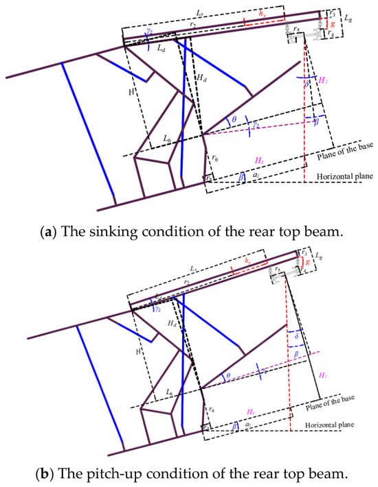
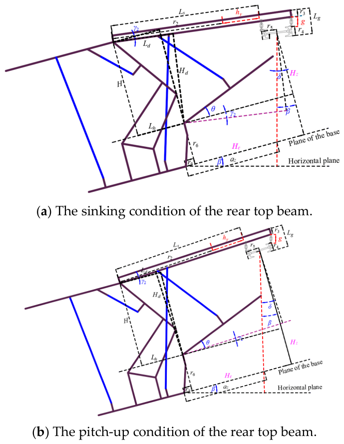
The posture of the backfill support robot was subjected to many complex factors. However, geometrical and motion constraints among the internal components of the robot remained unchanged within a certain range. Based on this principle, this study focused on the ZC5160/30/50 solid backfill hydraulic support and the single middle trough of the matched bottom-discharging conveyor as the object. It analyzed the geometrical structure [20], as shown in Figure 4.

Figure 4. Relative posture relations between the mechanisms.

In this study, the porous bottom-discharging scraper conveyor was referred to as the conveyor. The relative posture relation between the conveyor and the compaction mechanism is established to characterize the indices.

4.2.2. Posture Characterization Index of the Conveyor

The relation of the swing angle with the inclination angles of the coal seam and the rear angle can be written as:

$$\delta =\beta +{\gamma }_2$$

(57)

The spacing of the conveyor frame (along the axis of the rear top beam), defined as the relative posture characterization index of the conveyor relative to the rear top beam, can be written as:

$$L_S=r_2+h_y+g\sin \left(\delta \right)$$

(58)

The vertical distance of the top beam of the conveyor (along the normal direction of the top surface of the rear top beam) can be written as:

$$L_g=r_3+r_4+g\cos \left(\delta \right)$$

(59)

Equations (58) and (59) jointly represent the conveyor’s posture relative to the rear top beam, and these two indices were geometrically perpendicular to each other.

The offset distance control index: the index characterizing the posture of the rear top beam relative to the hinge point between the compaction mechanism and the base. To be specific, the vertical distance between the hinge point of the compaction and the top beam was the value between Point O and Point C along the axial direction of the rear top beam, and the horizontal distance between the hinge point of the compaction and the top beam was the value between Point O and Point C along the axial direction of the rear top beam.

At γ₂ < 0, the two indices can be written as:

$$H_d=H\cos \left({\gamma }_2\right)-L_h\sin \left(\left|{\gamma }_2\right|\right)$$

(60)

$$L_d=L_h\cos \left({\gamma }_2\right)+H\sin \left(\left|{\gamma }_2\right|\right)$$

(61)

At γ₂ > 0, the two indices can be written as:

$$H_d=L_h\sin \left({\gamma }_2\right)+H\cos \left({\gamma }_2\right)$$

(62)

$$L_d=L_h\cos \left({\gamma }_2\right)-H\sin \left({\gamma }_2\right)$$

(63)

The position control index of the material falling point: characterized by the distance between the material falling point and the discharge centre for the robots with different postures, also referred to as the distance between the material falling point and the rear of the base.

$$a_z=H_c+H_z\tan \left(\beta \right)$$

(64)

where the intermediate variable should satisfy the following Equations (65) and (66).

At γ₂ > 0:

$$\left\{\begin{array}{l}{H}_z=H+\left(L_s+r_5\right)\sin \left({\gamma }_2\right)-\left(L_g-r_1-\raisebox{1ex}{$r_4$}\!\left/ \!\raisebox{-1ex}{$2$}\right.\right)\cos \left({\gamma }_2\right)+r_6\\ H_c=\left(L_s+r_5\right)\cos \left({\gamma }_2\right)+\left(L_g-r_1-\raisebox{1ex}{$r_4$}\!\left/ \!\raisebox{-1ex}{$2$}\right.\right)\sin \left({\gamma }_2\right)-L_h+r_7\end{array}\right.$$

(65)

At γ₂ < 0:

$$\left\{\begin{array}{l}{H}_z=H-\left(L_s+r_5\right)\sin \left({\gamma }_2\right)-\left(L_g-r_1-\raisebox{1ex}{$r_4$}\!\left/ \!\raisebox{-1ex}{$2$}\right.\right)\cos \left({\gamma }_2\right)+r_6\\ H_c=\left(L_s+r_5\right)\cos \left({\gamma }_2\right)-\left(L_g-r_1-\raisebox{1ex}{$r_4$}\!\left/ \!\raisebox{-1ex}{$2$}\right.\right)\sin \left({\gamma }_2\right)-L_h+r_7\end{array}\right.$$

(66)

5. Construction of the Kinematic Analysis Model and Simulation on the Virtual Prototype

5.1. Solution Methods for the Kinematic Equation and Module Development

5.1.1. Numerical Solution Method

This study focuses on kinematic modelling, posture-index construction and mechanical–hydraulic-control co-simulation of the solid backfilling support robot. To solve the nonlinear equations relating posture angles, posture indices and actuator strokes, a Newton–Raphson iterative framework is used, and a trust-region strategy is introduced to constrain the iteration step and improve convergence stability under changing initial conditions. The numerical method is used as an implementation tool for the kinematic solution module; comparative optimization among different algorithms is not treated as the main contribution of this paper.

The Newton-Raphson method is a nonlinear equation-solving method based on Taylor expansion. At the current point x_k, F(x) can be linearized by the first-order Taylor expansion:

$$F\left(x_k\right)+J\left(x_k\right)\left(x-x_k\right)=0$$

(67)

where J(x_k) denotes the Jacobian F(x) matrix at x_k. To solve the linear equation, the new iteration point can be obtained:

$$x_{k+1}=x_k-J{\left(x_k\right)}^{-1}F\left(x_k\right)$$

(68)

The above procedure is repeated until the convergence criterion is satisfied. The Newton–Raphson method converges rapidly near the solution, but it is sensitive to the initial value and may become unstable when the iteration is far from the solution or close to singular configurations. To improve the stability of the iterative process, a trust-region strategy is introduced to regulate and correct the Newton step.

By considering the minimization problem min f(x), the quadratic approximation model was established at the current point x_k:

$$x_k\left(d\right)=f\left(x_k\right)+\nabla f{\left(x_k\right)}^{T}d+{\displaystyle \frac{1}{2}}{d}^T{H}_{k}d$$

(69)

where H_k denotes the Hessian matrix of f(x) at x_k (or the approximation); $\nabla$f(x_k) denotes the gradient vector of the objective function at x_k; d denotes the tentative step from x_k. Next, the sub-problem in the trust region was solved:

$${\min }_{\left(d\in R^n\right)} m_k \left(d\right),\parallel d\parallel \le {\Delta }_k$$

(70)

The tentative step d_k was obtained. According to the performance, whether to accept the tentative step and update the radius of the trust domain Δ_k can be judged. If the tentative step can be accepted, x_k+1 = x_k + d_k; otherwise, x_k+1 = x_k was maintained, and the radius of the trust domain was narrowed for solving the sub-problem.

Based on the above numerical solution method, the forward and inverse kinematic equations of the backfilling support robot can be implemented in the posture solution module. The numerical solver is used to support posture-index calculation and co-simulation control rather than to demonstrate superiority over heuristic optimization algorithms. The numerical implementation settings used in the MATLAB/Simulink kinematic modules are summarized in Table 3. The nonlinear residual tolerance was set to 1.0 × 10⁻⁶, the maximum number of iterations was 100, and the finite-difference perturbation for angular variables was 1.0 × 10⁻⁶ rad. The initial values of the main-loop variables were set to 50°, 139°, 43°, 137° and 94°. The initial values of the rear top-beam and swing/compaction subloops were set to 70° and 120°, respectively. These settings were kept unchanged in the forward, inverse and workspace-sampling verification. The initial values, convergence tolerance, finite-difference perturbation and co-simulation step size used for numerical implementation are also listed in Appendix A.

Table 3. Numerical settings used in the kinematic solution and co-simulation modules.

Item	Value
Nonlinear solver	Newton–Raphson with trust-region correction
Maximum iterations	100
Residual tolerance	1.0 × 10−6
Finite-difference perturbation	1.0 × 10−6 rad
Main-loop initial values	50°, 139°, 43°, 137°, 94°
Rear top-beam subloop initial value	70°
Swing/compaction subloop initial value	120°
Co-simulation solver	Fixed-step ode4 (Runge–Kutta)
Co-simulation communication step	0.01 s

5.1.2. Development of the Posture Solution Output Module

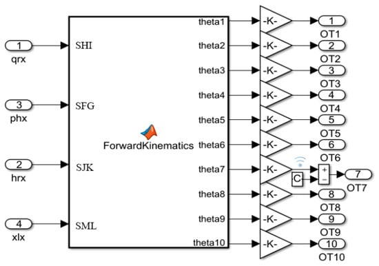
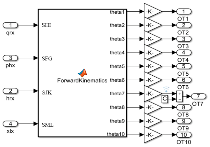
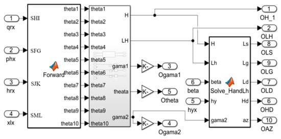
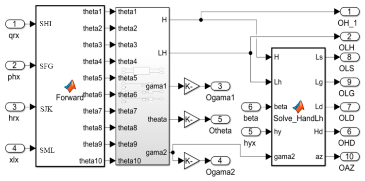
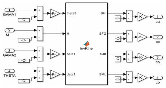
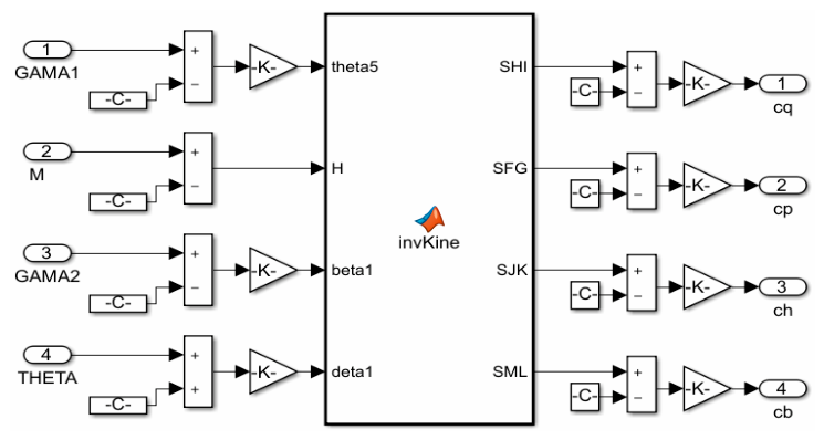
The kinematic analysis function of the backfill support robot is the foundation for achieving further complex functions. Based on the robot’s kinematic equation described in Section 2, forward and inverse kinematic solution problems were implemented and achieved in the Simulink MATLAB Function module, as the integrated Simulink models listed in Figure 5, Figure 6 and Figure 7.

Figure 5. Simulink module for kinematic forward solution.

Figure 6. Posture-index solution Simulink model for the backfill support robot.

Figure 7. Simulink module for inverse kinematic solution of the four-actuator posture-control subsystem.

In Figure 5: The ‘qrx’, ‘phx’, ‘hrx’, and ‘xlx’ corresponding to input ports 1–4 represent the lengths (unit: mm) of the hydraulic support’s front column, balance cylinder, rear column, and Swing cylinder, respectively. When ‘SHI’, ‘SJK’, ‘SFG’, and ‘SML’ appear at the input terminal, they denote actual measured values; when located at the output terminal, they represent the calculated desired values.

(1)

Forward solution: The left side of the module is the data input interface. The displacement data of each driving cylinder are transmitted to the kinematic solution module, and the calculated posture angles are output on the right side.

(2)

Posture-index solution module: Based on the ten posture angles obtained from the forward kinematic solution, the established posture indices can be calculated. In addition to structural parameters, the base inclination beta and the displacement hy of the rear telescopic mechanism are collected, while the remaining indices are obtained from the kinematic analysis module.

(3)

Inverse solution: In the posture-control branch, the target posture indices are transmitted to the inverse kinematic module through the left input ports, and the corresponding target strokes of the front column, balance cylinder, rear column and swing cylinder are output through the right ports. These four actuators form the main posture-control subsystem. The compaction-cylinder stroke is not included in this four-actuator posture-control branch; it is determined separately according to the prescribed compaction-plate terminal position, cylinder stroke or compaction-operation target.

5.2. Posture Solution Simulation Test

5.2.1. Test on the Kinematic Forward Solution Model

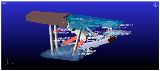
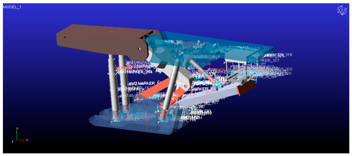
Figure 8 shows the mechanical system and kinematic analysis models of the intelligent solid backfill support robot, as established using ADAMS, MATLAB, and the joint simulation interface technology [19].

Figure 8. Mechanical model of the developed intelligent solid backfill support robot.

In the forward-kinematic numerical check, the ADAMS virtual prototype was first driven by the front column, balance cylinder, rear column and swing cylinder. The actuator lengths L_HI, L_FG, L_JK and L_LM and the posture angles θ₁–θ₁₀ were monitored. The actuator lengths were then imported into the MATLAB/Simulink forward-kinematic module to calculate the corresponding posture angles, which were compared with the ADAMS monitoring values. The comparison shows good consistency between the kinematic solution and the virtual-prototype output, indicating that the closed-loop vector model and the Simulink solution module can represent the geometric motion relationship of the virtual prototype. These errors describe numerical consistency between two models and should not be interpreted as physical prototype accuracy or underground measurement accuracy.

5.2.2. Test on the Posture-Index Solution Model

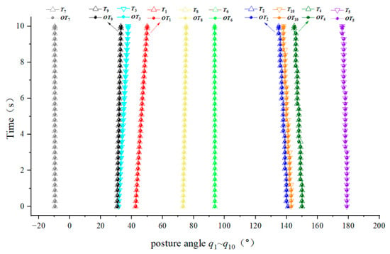
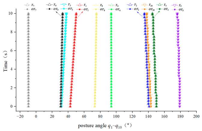
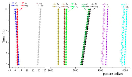
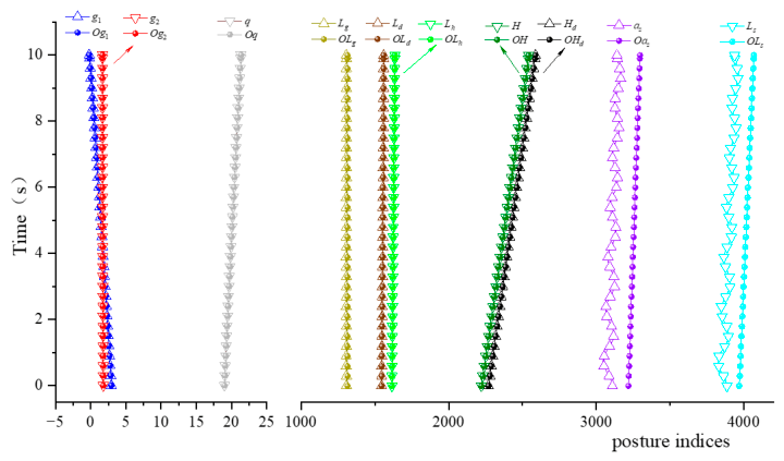
Five indices for characterizing the postures of the top beam and the compaction mechanism, H, L_h, γ₁, γ₂, and θ, and five indices for characterizing the relative position among the compaction mechanism, the rear top beam, and the conveyor, L_s, L_g, L_d, H_d, and a_z, were supplemented in ADAMS. The posture indices to be solved were denoted as OH, OL_h, Oγ₁, Oγ₂, Oθ, OL_s, OL_g, OL_d, OH_d, and Oa_z.

The comparison between the ADAMS-monitored and algorithm-solved posture-angle trajectories is shown in Figure 9.

Figure 9. Comparison between the monitored and the solution results of the posture angle θ₁–θ_10.

Figure 9 Comparison between the monitored and the solution results of the posture angle θ₁–θ₁₀. For the continuous posture-angle trajectories θ₁–θ₁₀, the RMSE between the algorithm-solved angles and the ADAMS-monitored angles ranged from 0.0007° to 0.0651°, indicating good trajectory-level consistency of the solved mechanism angles.

As shown in Figure 10 and Table 4, the calculated values of the top-beam inclinations, compaction angle and most key distance indices agree with the monitored values. To avoid overinterpreting the numerical comparison, the errors of each distance-type posture-index were further quantified using the mean absolute error (MAE), maximum absolute error and relative error, as summarized in Table 5. The results show that the main rigid-body posture indices, including H, L_h, L_d and H_d, have small numerical differences between the analytical solution and the ADAMS monitoring results. In contrast, the conveyor-related indices Ls and a_z show larger deviations, with maximum absolute errors of 140 mm and 166 mm, respectively. This difference is mainly attributed to the gravity-induced swing of the suspended backfilling scraper conveyor in the ADAMS virtual prototype, which is not fully represented in the geometric kinematic model. Therefore, the comparison should be interpreted as a numerical consistency check of the kinematic model rather than as evidence of physical measurement accuracy.

Figure 10. Comparison between the monitored and the solution results of the posture indices.

Table 4. Comparison of the monitored and calculated results for selected posture indices (in mm).

H	OH	Lh	OLh	Ls	OLs	Lg	OLg	Ld	OLd	Hd	OHd	az	Oaz
2221.43	2221.46	1615.49	1615.66	3886	3970	1307	1314	1545.59	1545.74	2270.62	2270.67	3110	3219
2254.00	2254.04	1617.43	1617.61	3843	3980	1306	1314	1547.40	1547.55	2302.65	2302.70	3065	3227
2286.47	2286.50	1619.41	1619.59	3863	3990	1306	1314	1549.17	1549.33	2334.64	2334.69	3083	3235
2318.82	2318.86	1621.41	1621.59	3907	4000	1307	1314	1550.88	1551.04	2366.58	2366.63	3125	3242
2351.05	2351.09	1623.42	1623.61	3870	4010	1306	1314	1552.51	1552.67	2398.47	2398.52	3084	3250

Table 5. Error statistics of selected distance-type posture indices.

Index	MAE/mm	Maximum Absolute Error/mm	Relative Error/%
H	0.036	0.040	0.00157
Lh	0.180	0.190	0.0111
Ls	116.200	140.000	2.9996
Lg	7.600	8.000	0.5818
Ld	0.156	0.160	0.0101
Hd	0.050	0.050	0.00214
az	141.200	166.000	4.5646

5.2.3. Test on the Kinematic Inverse Solution Model

A representative inverse kinematic case was first used to check whether the target posture indices could be converted into actuator lengths and then recovered by the posture-index solution module. The prescribed posture indices γ₁, γ₂, M and θ were input into the inverse kinematic module, and the solved actuator lengths were applied to the forward/posture-index solution module for comparison. The target posture inputs and the corresponding expected actuator lengths are listed in Table 6, and the recovered posture indices after applying these actuator lengths are listed in Table 7.

Table 6. Target posture inputs and expected actuator lengths.

Posture Index	Value	Expected Mechanism Type	Length (mm)
γ1	−5°	SHI	3960.432
γ2	−5°	SFG	1238.726
M	4000 mm	SJK	3145.346
θ	25°	SML	2300.455

Table 7. Monitored posture indices after applying the expected actuator lengths.

Actuator	Expected Length of the Mechanism (mm)	Posture Index	Solution Value
SHI	3960.432	γ1	−4.99°
SFG	1238.726	γ2	−4.99°
SJK	3145.346	H	2800.00 mm
SML	2300.455	θ	24.99°

The difference between H and M was 1200 mm, corresponding to the sum of the top-beam thickness and the distance from the rear-hinge-rod hinge point to the base plane. As shown in Table 6 and Table 7, the recovered posture indices agree with the target values, indicating that the inverse kinematic module is numerically consistent for this representative case.

To further examine the numerical robustness of the inverse kinematic solution, a representative workspace sampling test was added. Fifteen target postures were generated from five support heights (H = 2400, 2500, 2600, 2700 and 2800 mm) and three posture modes (neutral, positive-inclination and negative-inclination modes). For each target posture, the inverse kinematic model was used to calculate the four main posture-control actuator lengths, and the obtained lengths were then substituted into the forward-kinematic model for inverse–forward round-trip verification. Stroke constraints were also checked for the front column, balance cylinder, rear column and swing cylinder.

The 15-case inverse–forward workspace sampling verification is summarized in Table 8. All 15 cases converged successfully and satisfied the actuator stroke constraints. The minimum stroke margin was 122.256 mm. The maximum round-trip error was 1.287 × 10⁻⁸° for the posture angles and 4.038 × 10⁻⁹ mm for the support height or M index. These results indicate numerical consistency between the inverse and forward kinematic models within the sampled representative workspace. The sampling test was used to evaluate representative numerical robustness and should not be interpreted as exhaustive coverage of the entire workspace.

Table 8. Summary of the 15-case inverse–forward workspace sampling verification.

Item	Result
Number of target postures	15
Height levels H/mm	2400, 2500, 2600, 2700, 2800
Posture modes	Neutral, positive, negative
Converged cases	15
Stroke-feasible cases	15
Minimum stroke margin/mm	122.256
Maximum angle round-trip error/°	1.287 × 10−8
Maximum height/M round-trip error/mm	4.038 × 10−9
Front-column solved range/mm	2730.617–3384.705
Balance-cylinder solved range/mm	1174.183–1322.744
Rear-column solved range/mm	2562.654–3223.176
Swing-cylinder solved range/mm	1999.946–2385.143

6. Test on the Posture Control of the Backfill Support Robot

6.1. Mechanical-Electrical–Hydraulic Integrated Joint Simulation Model

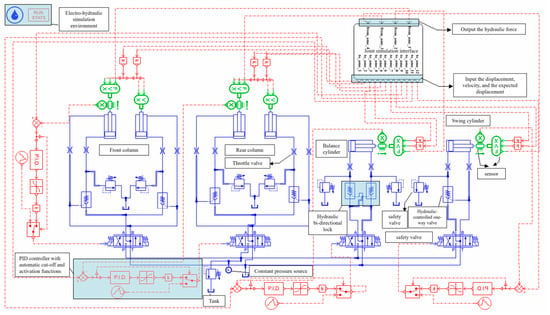
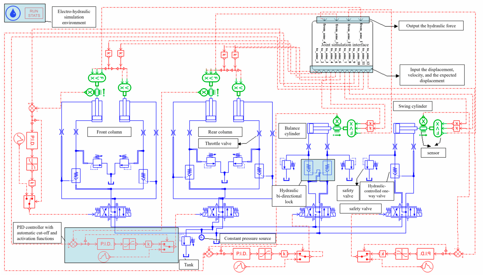
Based on the ADAMS mechanical model, the AMESim hydraulic system model and the MATLAB/Simulink kinematic solution modules, a mechanical–hydraulic-control co-simulation platform was constructed, as shown in Figure 11. The simulations and control modules were implemented using ADAMS 2020, Simcenter Amesim 2020 and MATLAB/Simulink 2019. ADAMS provides the mechanical motion states of the robot, including actuator lengths, key hinge positions and monitored posture angles. MATLAB/Simulink performs forward and inverse kinematic calculations and posture-index calculation, and outputs the target actuator lengths or calculated posture indices. AMESim simulates the hydraulic actuator response and outputs the actual cylinder displacement, valve-controlled execution process and tracking curves.

Figure 11. Dynamic and control system model of the intelligent solid backfill support robot.

The fixed communication step used in the co-simulation is adopted for synchronized data exchange among the software modules and should not be interpreted as the physical control period of a real controller. In the AMESim hydraulic model, a constant-pressure hydraulic source of 315 bar was used. The hydraulic cylinder parameters of the four posture-control actuators are listed in Table 9. The four posture-control actuators were driven by valve controlled hydraulic branches. The hydraulic valve flow parameters used in the co-simulation model are listed in Table 10. The maximum flow settings of the valves were defined under a nominal valve pressure drop of 20 bar. The flow rates of the reversing valves were set to 200 L/min for the front column, balance cylinder and rear column, and 600 L/min for the swing cylinder. The rod/bore diameters of the front column, rear column, balance cylinder and swing cylinder were 230/250 mm, 230/250 mm, 160/180 mm and 85/140 mm, respectively. The dead volumes at the two cylinder ports were set to 50 cm³, and the viscous friction coefficient was set to 10,000 N/(m/s). The load in the reported control cases was generated mainly by the self-weight of the top beams, linkages and hydraulic cylinders in the ADAMS mechanical model; no additional calibrated roof-contact disturbance load was applied.

Table 9. Hydraulic-cylinder parameters of the four posture-control actuators.

Actuator	Rod Diameter/mm	Bore Diameter/mm	Stroke Range/mm
Front column	230	250	2400–4395
Rear column	230	250	2320–4205
Balance cylinder	160	180	935–1445
Swing cylinder	85	140	1515–2715

Table 10. Hydraulic valve flow parameters used in the co-simulation model.

Actuator	Maximum Flow Rate of Reversing Valve/L·min−1	Nominal Pressure Drop/bar
Front column	200	20
Balance cylinder	200	20
Rear column	200	20
Swing cylinder	600	20

The controller used in this study was the PID control module in AMESim, with the PID parameter settings shown in Table 11.

Table 11. PID controller parameters used in the hydraulic actuator tracking model.

Mechanism	P	I	D
Front column	6500	0	0
Balance cylinder	890	0	0
Rear column	7400	0	0
Swing cylinder	3200	0	20

The PID controller was used to evaluate the feasibility of actuator-length tracking in the co-simulation framework, rather than to compare different advanced control algorithms.

6.2. Posture-Control Test Scheme and Evaluation Metrics

Posture-control principle: Based on the inverse kinematics relationship, the corresponding relationship between the target posture and the movement amount of the driving cylinder can be established. A posture index can characterize the target posture. Meanwhile, the target value of the driving cylinder can be inversely solved from the posture index and then tracked and executed by the controller.

In the co-simulation framework, the posture-control process consists of four stages: target posture specification, inverse kinematic mapping, hydraulic actuator tracking and posture-index feedback. First, the prescribed posture indices are converted into the target lengths of the four posture-control actuators by the inverse kinematic module. Second, the target length of each actuator is transmitted to the AMESim hydraulic control model. Third, the PID controller drives the valve-controlled hydraulic actuator to track the target length. Finally, the actuator displacements and posture indices monitored from ADAMS are fed back for error evaluation.

For the i-th actuator, the length-tracking error is defined as e_i(t) = L_i,ref(t) − L_i(t), where L_i,ref(t) is the target actuator length obtained from inverse kinematics and L_i(t) is the monitored actuator length in the co-simulation. The integral of time-weighted absolute error is calculated as $ITA{E}_i={\displaystyle {\int }_{t_0}^{t_f}t}|e_i(t)|dt$. In the present data processing, t₀ was set to 0.01 s because the t = 0 reference-initialization row was excluded. Controller performance was evaluated using RMSE, ITAE, maximum absolute error, steady-state error, maximum overshoot and settling time.

Test scenario: During the lifting process, the support robot should adjust the inclination angle of the top beam in advance based on the posture of the roof to ensure smooth contact.

Height variation range: The support height M varies from 4000 mm to 4500 mm in the control cases.

Target posture 1 is a pitch-down posture, with γ₁ = γ₂ = 5° and θ = 25°.

Target posture 2 is a pitch-up posture, with γ₁ = γ₂ = −5° and θ = 25°.

6.3. Posture-Control Test Results

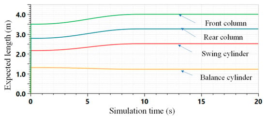
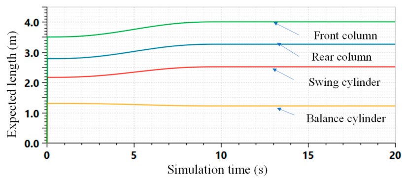
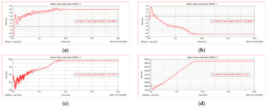
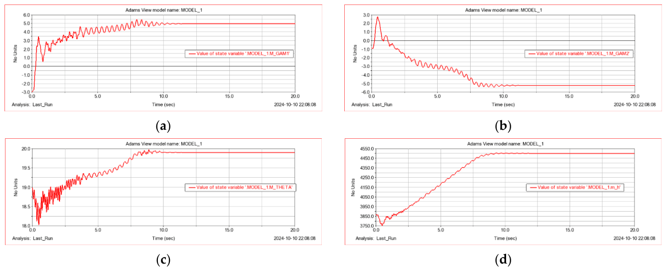
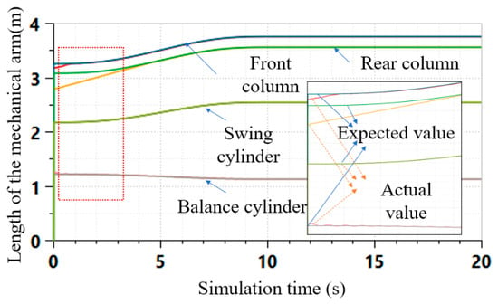
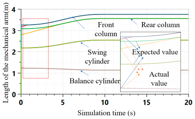
The target posture parameters of the two cases were imported into the inverse kinematic module to obtain the expected actuator-length trajectories, which were then transmitted to the AMESim hydraulic control model. A representative set of expected actuator-length curves is shown in Figure 12, and the monitored posture-index curves of target posture 1 are shown in Figure 13. By comparing the target and monitored values, the posture errors after PID control were obtained and are summarized in Table 12.

Figure 12. The expected length curve of each drive cylinder under the target posture 1 (monitored in AMESim).

Figure 13. Monitored values of various posture indices under the target posture 1. (a) Monitored value of the inclination angle of the front top beam γ₁. (b) Monitored value of the inclination angle of the front top beam γ₂. (c) Monitored value of the compaction angle for the compaction mechanism θ. (d) Monitored value of the height of the backfill support robot M.

Table 12. Steady-state errors of posture indices in two target posture cases.

Error	Target Posture 1	Target Posture 2
Δγ1	−0.0394°	−0.1404°
Δγ2	0.2139°	−0.0435°
Δθ	−0.1002°	−0.1397°
Δh	0.86 mm	4.16 mm

The simulations were also performed on target posture 1 and target posture 2. Posture indices were monitored, as shown in the curve of target posture 1 in Figure 13.

By comparing the monitored and the expected values, the motion errors of the mechanism driven by the PID controller were obtained and summarized in Table 12.

By adjusting the parameters of the PID controller, the controller was enabled to respond quickly and stably track the expected displacement curve, as shown in the initial debugging results in Figure 14.

Figure 14. Tracking execution performance of the PID controller.

As shown in Figure 14 and Table 13, the target-actual actuator tracking data further quantify the hydraulic execution performance of the four posture-control actuators. Because the reference signals at t = 0 were initialized to zero in the exported data, the error statistics were calculated from t = 0.01 s. In both target posture cases, all actuator lengths remained within their allowable stroke ranges, and the steady-state tracking errors were below 2.4 mm. The maximum overshoot did not exceed 5.58%. Larger RMSE and ITAE values were observed for the front column in Pose 1 and the rear column in Pose 2, mainly because these actuators had larger displacement demands and longer response delays under the hydraulic flow constraints. These results indicate that the co-simulation framework can identify not only kinematic feasibility but also hydraulic execution delay and flow-limited tracking behaviour.

Table 13. Quantitative tracking performance of the four posture-control actuators.

Case	Actuator	RMSE/mm	ITAE/mm·s2	Max. Abs. Error/mm	Steady-State Error/mm	Max. Overshoot/%	Settling Time/s	Stroke Status
Pose 1, pitch-down	Rear column	10.242	223.432	82.493	0.316	0.140	0.74	Within range
Pose 1, pitch-down	Front column	66.332	761.931	293.185	0.179	0.056	4.04	Within range
Pose 1, pitch-down	Balance cylinder	4.534	501.222	39.244	2.368	1.004	10.20	Within range
Pose 1, pitch-down	Swing cylinder	0.966	76.643	3.353	0.099	0.034	0.01	Within range
Pose 2, pitch-up	Rear column	94.155	2685.261	335.923	0.194	0.087	7.62	Within range
Pose 2, pitch-up	Front column	2.788	192.069	11.291	0.334	0.045	1.47	Within range
Pose 2, pitch-up	Balance cylinder	6.862	458.153	54.841	2.015	5.578	—	Within range
Pose 2, pitch-up	Swing cylinder	9.622	75.236	138.900	0.099	0.058	0.30	Within range

Note: The t = 0 reference-initialization row was excluded. The settling time of the balance cylinder in Pose 2 is not reported because it did not enter and remain within the adopted tolerance band, although its steady-state error was 2.015 mm.

6.4. Discussion

This study also has limitations. The present verification is based mainly on virtual-prototype and co-simulation results, without laboratory prototype or underground field data. Joint clearance, hydraulic leakage, seal friction, structural flexibility, roof-load disturbance and sensor noise are not fully represented in the current model. In addition, the PID controller is used to check the feasibility of the posture-control process and is not compared systematically with active disturbance rejection control, sliding-mode control, fuzzy PID or model predictive control. Future work will calibrate the model using prototype experiments and field tests and will introduce adaptive control methods for strongly disturbed mining conditions.

In the reported control cases, the mechanical load was mainly generated by the self-weight of the robot components in the ADAMS model. Calibrated roof-contact load distribution and dynamic coal-rock disturbance were not introduced; therefore, the force-mapping equations should be interpreted as a theoretical interface rather than a validated working-resistance design.

Compared with a purely mechanical virtual prototype, the ADAMS-AMESim-MATLAB/Simulink co-simulation can describe mechanism motion, hydraulic response and controller execution simultaneously. The delayed response of the front column indicates that kinematic reachability does not guarantee immediate hydraulic execution. Therefore, control-system design for large hydraulic mining robots should consider geometric reachability, hydraulic flow limits and mechanism coupling together.

The results show that the closed-loop vector method can describe the geometric coupling among the front top beam, rear top beam and compaction mechanism of the solid backfilling support robot. Through the posture-index system, the complex mechanism motion is transformed into engineering-oriented state variables that can support roof-contact, backfilling and compaction-state analysis.

7. Conclusions

The main conclusions are as follows:

(1)

Closed-loop vector equations were established for the front mechanism, rear top-beam mechanism and compaction mechanism of the solid backfilling support robot. The model describes the mapping relationships among actuator strokes, posture angles and key node positions, and can represent the geometric coupling among the dual top beams, multiple linkages and compaction mechanism.

(2)

A posture-index system was constructed for roof-contact, support and backfilling operations. The indices include the inclinations of the front and rear top beams, hinge-point height, compaction mechanism angle and relative-position indices between the conveyor and the compaction mechanism. This index system provides a unified variable interface for posture calculation, state monitoring and control input.

(3)

Forward and inverse kinematic modules and posture-index calculation modules were implemented in MATLAB/Simulink and checked using an ADAMS virtual prototype. The main rigid-body posture indices showed good numerical consistency, whereas the conveyor-related relative-position indices showed larger deviations because the suspended conveyor motion was affected by gravity in the virtual prototype. A 15-case inverse–forward sampling verification further showed successful convergence, feasible actuator strokes and negligible round-trip errors. The residual Jacobian analysis showed that all sampled postures retained full rank, with maximum condition numbers of 9.135–9.950.

(4)

A mechanical–hydraulic-control co-simulation platform was established by coupling ADAMS-AMESim-MATLAB/Simulink. Under two target posture cases, the PID-controlled posture deviations of the top beams and compaction mechanism were within ±0.3°, and the height deviation was less than 5 mm. The actuator-level target-actual tracking results showed that all four posture-control actuators remained within their stroke ranges, with steady-state tracking errors below 2.4 mm and maximum overshoot below 5.58%. These results indicate that the proposed co-simulation workflow can be used to analyze posture adjustment and hydraulic execution feasibility of the solid backfilling support robot.

(5)

The verification results mainly reflect model-level numerical consistency and control-process feasibility in a simulation environment. They should not be interpreted as physical prototype accuracy or field validation. Future research will combine laboratory prototype tests and underground industrial tests to further consider calibrated roof-contact loads, joint clearance, hydraulic leakage, friction, structural flexibility, coal-rock disturbance and sensor noise.

References

- Zhang, J.X.; Zhang, Q.; Zhou, N.; Li, M.; Huang, P.; Li, B. Research progress and prospect of coal based solid waste backfilling mining technology. J. China Coal Soc. 2022, 47, 4167–4181. [Google Scholar]
- Liu, J.G.; Li, X.W.; He, T. Application status and prospect of backfill mining in Chinese coal mines. J. China Coal Soc. 2020, 45, 141–150. [Google Scholar]
- Liu, F.; Guo, L.F.; Zhang, J.M.; Wang, L. Synergistic mode of digitalization-intelligentization-greeniation of the coal industry and its path of building new coal productivity. J. China Coal Soc. 2024, 49, 1–15. [Google Scholar]
- Ge, S.R.; Zhang, X.; Xue, G.H.; Ren, H.; Wang, H.; Pang, Y.; Fan, L. Development of intelligent technologies and machinery for coal mining in China’s underground coal mines. Strateg. Study CAE 2023, 25, 146–156. [Google Scholar] [CrossRef] [Scilit]
- Huang, Z.; Ge, S.; He, Y.; Wang, D.; Zhang, S. Research on the intelligent system architecture and control strategy of mining robot crowds. Energies 2024, 17, 1834. [Google Scholar] [CrossRef] [Scilit]
- Ge, S.R.; Hu, E.Y.; Li, Y.W. New progress and direction of robot technology in coal mine. J. China Coal Soc. 2023, 48, 54–73. [Google Scholar]
- Wang, G.F.; Pang, Y.H.; Ren, H.W.; Zhan, K.; Du, M.; Zhang, Y.; Cheng, J.; Du, Y.; Zhang, J.; Gong, S. System engineering and key technologies research and practice of smart mine. J. China Coal Soc. 2024, 49, 181–202. [Google Scholar]
- Shi, P.; Zhang, J.; Yan, H.; Zhang, Y.; Zhang, Q.; Feng, W. Evaluation of operating performance of backfilling hydraulic support using six hybrid machine learning models. Minerals 2022, 12, 1388. [Google Scholar] [CrossRef] [Scilit]
- Zhang, Q.; Shi, P.; Li, M.; Zong, T.; Song, W. A design method and application of backfilling hydraulic supports in reforming top-coal caving hydraulic supports. Appl. Sci. 2023, 13, 987. [Google Scholar] [CrossRef] [Scilit]
- Zeng, Q.L.; Ban, X.L.; Meng, Z.S.; Wan, L.; Lei, X. Digital twin reconstruction method of group spatial support pose for hydraulic support of working face based on Unity3D. Coal Sci. Technol. 2024, 52, 77–88. [Google Scholar]
- Pang, Y.H.; Liu, X.H.; Wang, H.B.; Jiang, Z.; Guan, S.; Zhang, Z.; Wang, W. Support attitude and height analysis method of hydraulic support based on jack stroke drive. J. Min. Saf. Eng. 2023, 40, 1231–1242. [Google Scholar]
- Zhang, Y.; Zhang, H.; Gao, K.; Zeng, Q.; Meng, F.; Cheng, J. Research on intelligent control system of hydraulic support based on position and posture detection. Machines 2023, 11, 33. [Google Scholar] [CrossRef] [Scilit]
- Zhang, Y.; Zhang, H.; Gao, K.; Xu, W.; Zeng, Q. New method and experiment for detecting relative position and posture of the hydraulic support. IEEE Access 2019, 7, 181842–181854. [Google Scholar] [CrossRef] [Scilit]
- Du, Y.B. Supporting condition acquisition and fuzzy comprehensive evaluation method for hydraulic support. J. China Coal Soc. 2017, 42, 260–266. [Google Scholar]
- Ren, H.W.; Li, S.S.; Zhao, G.R.; Zhang, K.; Du, M.; Zhou, J. Measurement method of support height and roof beam posture angles for working face hydraulic support based on depth vision. J. Min. Saf. Eng. 2022, 39, 72–81. [Google Scholar]
- Wang, Y.; Shi, Y.N.; Wang, Y.Y.; Qi, P.; Wang, H. Full pose measurement and virtual simulation of solid filling hydraulic support. J. Mine Autom. 2022, 48, 81–89. [Google Scholar]
- Yan, H.F. Study on Key Techniques of Hydraulic Support Virtual Monitoring System. Ph.D. Thesis, China University of Mining & Technology, Xuzhou, China, 2011. [Google Scholar]
- Zhang, L. Research on Key Technologies of Autonomous Following Mining Machine for Hydraulic Support. Ph.D. Thesis, China University of Mining & Technology, Xuzhou, China, 2017. [Google Scholar]
- Lin, F.Y.; Miao, C.Q. Resolution on motion posture of chock-shield type hydraulic powered support. Coal Sci. Technol. 2011, 39, 97–100. [Google Scholar]
- Lu, X.L.; Yan, H.F.; Zhang, L. Inverse kinematics analysis of hydraulic support. Ind. Mine Autom. 2018, 44, 43–47. [Google Scholar]
- Meng, Z.S.; Zeng, Q.L.; Wan, L.R.; Liu, P. Pose adjusting simulation of hydraulic support based on mechanical-electrical-hydraulic coordination. Teh. Vjesn.-Tech. Gaz. 2018, 25, 1110–1118. [Google Scholar] [CrossRef] [Scilit]
- Zeng, Q.; Hu, Y.; Meng, Z.; Wan, L. Research on velocity feedforward control and precise damping technology of a hydraulic support face guard system based on displacement feedback. Machines 2024, 12, 676. [Google Scholar] [CrossRef] [Scilit]
- Hou, T.; Kou, Z.; Wu, J.; Xu, P.; Zhang, B.; Peng, Y. Positioning control strategy of hydraulic support pushing system in fully mechanized coal face. Electronics 2023, 12, 3628. [Google Scholar] [CrossRef] [Scilit]
- Sun, M.Z.; Wang, Y.Q.; Chang, Y.J.; Zhu, D.; Li, S.; Yang, K. Distributed cooperative control of consistency of hydraulic support robot group moving frame. J. China Coal Soc. 2024, 49, 1208–1222. [Google Scholar]
- Zhang, Q.; Zhang, J.X.; Zong, T.C.; Yang, K.; Jin, Z.; Lyu, H.; Bai, Y.; Deng, P. Intelligent solid backfilling support robot in coal mine and its key technology. J. China Coal Soc. 2025, 50, 1376–1392. [Google Scholar]
- Zong, T.C.; Zhang, Q.; Shi, P.T.; Wang, Y.; Li, F.; Chang, T. Mechanism interference critical characterization and autonomous demodulation method of solid filling hydraulic support. Coal Sci. Technol. 2023, 51, 260–270. [Google Scholar]
Disclaimer/Publisher’s Note: The statements, opinions and data contained in all publications are solely those of the individual author(s) and contributor(s) and not of MDPI and/or the editor(s). MDPI and/or the editor(s) disclaim responsibility for any injury to people or property resulting from any ideas, methods, instructions or products referred to in the content. |
© 2026 by the authors. Licensee MDPI, Basel, Switzerland. This article is an open access article distributed under the terms and conditions of the Creative Commons Attribution (CC BY) license.