


Abstract
The demand for robotic manipulators has increased because of their precision, speed, and cost-efficiency in complex or hazardous tasks. Flexible robotic manipulators, unlike rigid ones, offer lower mass and energy consumption, enabling advanced applications across various fields. Despite these advantages, the mass reduction of these manipulators can lead to undesired effects, including decreased precision, increased sensitivity to parametric uncertainties, coupled dynamics, and increased oscillations caused by their inherent flexibility. Moreover, the modeling complexity of such mechanical systems represents a significant challenge, since multiple degrees of freedom must be considered. In this study, a physics-informed neural network (PINN) is designed to estimate the dynamic behavior of a flexible-link manipulator. First, a dataset is created by executing different trajectories (i.e., different rotation angles) of the flexible manipulator. Based on the dataset, the PINN is then trained using time and strain signals as inputs to estimate the angular displacement, combining a data-driven loss with a physics-based loss derived from the system’s dynamic model. Finally, the PINN model is investigated experimentally to assess the closed-loop strategy and evaluate its efficiency and reproducibility in recognizing the mechanical system behavior. Therefore, the results show that the PINN and closed-loop experimental validations are consistent with the proposed method.
1. Introduction
In recent years, demand for robotic manipulators has increased significantly across large-scale industries and manufacturing plants, particularly for tasks that are hazardous, repetitive, or complex for human operators. Robotic manipulators have gained increasing interest due to their precision, speed, and cost-effectiveness [1,2]. Two main types of robotic manipulators, based on their structural configuration, are commonly used: rigid-link and flexible-link manipulators. Although rigid-link manipulators are widely used in industrial plants, they often require higher manufacturing costs, increased energy consumption (due to the presence of large actuators), and lower operational speeds. Lightweight flexible-link manipulators, in turn, have emerged as a promising alternative, addressing several of these limitations [3]. Their lower mass and smaller actuators enable a wide range of applications, including space-based operations, agricultural automation, and precision tasks such as robotic welding [4].
However, reducing the mass of robotic manipulators can introduce undesired effects, including decreased precision, increased sensitivity to parametric uncertainties, and significant oscillations attributable to their inherent flexibility [5]. Moreover, their dynamics are intrinsically complex because of time-varying behavior, non-minimum-phase characteristics, strong nonlinearities, multiple degrees of freedom, and complexity of equations [6]. Several methodologies have been investigated for modeling and designing a flexible robotic manipulator, including Hamiltonian Principle, Newton–Euler equations, the lumped parameter method, the assumed mode method, and other approaches [7,8,9]. Despite their advantages, model-based approaches present trade-offs that may limit their applicability in certain scenarios, particularly due to their high complexity and inherent uncertainties. Moreover, the presence of multiple degrees of freedom adds to this complexity and hinders generalization, i.e., non-adapted. This limitation arises because large-scale models are necessary and demand substantial computational effort, rendering them unsuitable for real-time control.
Given this context, machine learning techniques emerge as promising alternatives for identifying complex and nonlinear patterns in flexible robotic manipulators. Among these, physics-informed neural networks (PINNs) have gained significant attention due to their ability to incorporate physical laws, typically expressed as partial differential equations (PDEs), directly into the training process. This approach is particularly advantageous in scenarios characterized by limited or sparse observational data because it leverages governing equations to constrain the solution space and enhance generalization [10]. Bao et al. (2021) [11] investigated the use of physics-guided neural network and sliding mode control for closed-loop model identification of two-joint and three-joint manipulators. The neural network was used to estimate and compensate for modeling errors online, while the physics-based model provided the fundamental system dynamics and stability analysis. The proposed strategy showed better trajectory tracking accuracy and disturbance rejection compared to conventional methods. Yang et al. (2023) [12] investigated the use of a physics-informed neural network (PINN) framework for modeling and identifying unknown dynamic parameters of collaborative robots during physical human–robot interaction. Two experiments were conducted to evaluate the proposed strategy for identifying the complete dynamic model of a flexible-joint robot. The results showed good agreement with the corresponding experimental data.
Wang et al. (2024) [13] investigated the use of a PINN for modeling complex deformation in a Fin Ray soft robotic gripper. By embedding the elastic mechanics principle of minimum potential energy into its loss function and augmenting it with a small number of high-fidelity experimental observations, the proposed strategy achieved an effective balance between physical grounding and data efficiency. The results demonstrated that the PINN strategy improved accuracy compared with a finite element model (FEM) when a data assimilation scheme was applied to address the sim-to-real gap. Soyleyici and Unver (2025) [14] assessed the use of a physics-informed deep neural network (PIDNN) framework for the simulation and parameter identification of vibrating beam structures. By embedding the beam’s governing equations into the neural network training process, the method simultaneously predicted the structural response and estimated unknown physical parameters with high accuracy. Experimental results revealed that the proposed strategy provided robust parameter identification, highlighting its potential for structural dynamics and health monitoring applications. Li and Xiao (2025) [15] assessed the design of a PINN-based input-shaping method for vibration suppression of flexible robotic arms. The optimal input-shaping parameters were identified during training to minimize residual vibration. The results indicated improved performance of the PINN method compared with conventional methods, such as the Zero Vibration and Zero Vibration Derivative methods, considering both single-mode and multimode scenarios.
Li et al. (2025) [16] used PINNs to model compliant robotic manipulators. The proposed strategy accounted for the complex nonlinear characteristics, enabling accurate construction of the inverse dynamics model for compliant manipulators. Likewise, Savio et al. (2025) [17] investigated the use of the PINN methodology for dynamic model and parameter identification. The PINN technique was developed using Kirchhoff’s equations and experimental data, resulting in the identification of model parameters and the derivation of a neural network model. Numerical results revealed that the PINN can estimate both the mechanical system dynamics and equivalent material properties, such as mass, inertia, and other parameters. In addition, Kan et al. (2025) [18] also assessed the use of the PINN methodology for parameter identification. The proposed strategy aims to identify coefficients, including mass, damping, and stiffness, that allow for adequate dynamic modeling of complex flexible systems. Based on the identified model, a non-singular terminal sliding mode controller (TSMC) is developed to investigate the vibration suppression of the mechanical system. Despite these recent applications of PINNs for system identification, closed-loop experimental validation remains limited for flexible robotic manipulators.
Few studies have demonstrated the use of PINNs for modeling and controlling flexible robotic manipulators. Furthermore, comparative analyses and generalized methodologies applicable to flexible manipulators are not yet well established within the field. This work presents a PINN framework for the identification of complex dynamic behaviors in flexible mechanical systems, exemplified through a flexible robotic manipulator. The motion of the flexible manipulator is modeled as a superposition of rigid-body kinematics and elastic characteristics arising from its low thickness and lightweight structure. Accurate modeling and control of flexible manipulators represent challenging tasks due to the nonlinear and coupled dynamics between rigid and flexible components. To address these issues, the proposed PINN architecture integrates prior physical knowledge encoded through governing equations with data acquired from experimental trajectories. A dataset is created from multiple reference trajectories executed under a dual-loop control scheme, by combining the control law of rigid (by rigid kinematics) and flexible (by strain gauge signals). The PINN strategy is then used to replace the kinematic equations, the use of filters, and flexible control. In addition, unknown parameters are used as decision variables in the physical loss function to investigate effects of flexibility. The main contributions of this work are (i) the development of a generalized PINN-based modeling approach for capturing the coupled dynamics of flexible-link manipulators and (ii) the closed-loop experimental validation of the proposed framework under realistic operating conditions.
The paper is organized as follows. Section 2 presents the methodology and instrumentation used for the proposed work. Section 3 details the dynamic modeling of the flexible link and the physics-informed neural network strategy. It also presents the generalized approach for flexible robotic manipulators. Section 4 presents both the dual-loop control strategy used to collect the data and the closed-loop approach designed to validate the PINN strategy. Section 5 presents the main results, highlighting the performance of the PINN strategy through closed-loop experimental validation, while Section 6 presents the final remarks.
2. Methodology
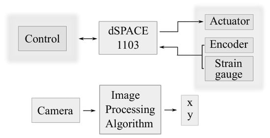
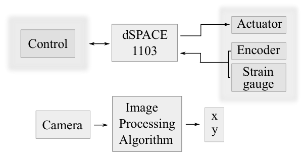
This section describes the flexible robotic manipulator and the equipment used. Figure 1 shows the instrumentation used between the equipment and the prototype. In this work, the prototype is formed by a single flexible link. Since this flexible manipulator has a serial kinematic configuration, a single kinematic chain is used to define the prototype. This single chain is formed by a flexible link and one active revolute joint, which is driven by a motor. The motor is used as the actuator to generate the desired movement of the mechanical prototype. In addition, the communication between the prototype and the computer interface is accomplished by a control board dSPACE 1103 (dSPACE GmbH, Paderborn, Germany), which can codify the measured signals and the motor current, by a corresponding control law.
Figure 1.
Scheme of the prototype communication.
Two sensors are used to acquire signals from the flexible link: an encoder and strain gauges. The encoder is responsible for measuring the angular rotation of the link, whereas the strain gauge is used to estimate the link’s flexibility in real-time. Note that, due to the low thickness of the manipulator, a significant contribution from the flexibility can be observed in the final dynamics. This combination of sensors enables the estimation of the final dynamic characteristics of the flexible link, by assuming that the encoder is enable to collect the rigid, and the strain gauge the flexible dynamics. Due to the limitations of previous sensors to capture the end of the flexible link, a camera is used as an additional and external sensor to calculate its position. The camera is combined with an image-processing algorithm to estimate the end-effector positions, and then compared with the proposed strategy.
Instrumentation Scheme
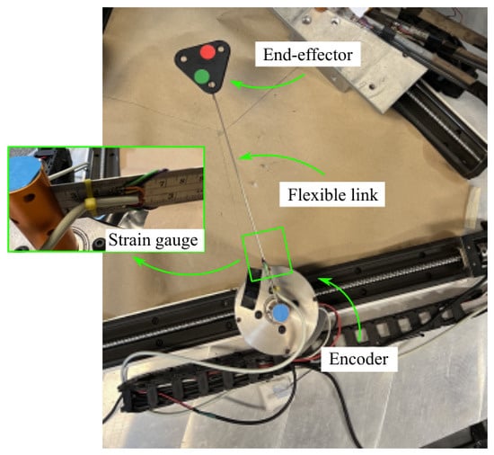
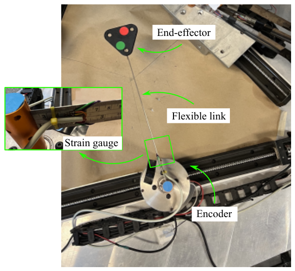
The flexible robotic manipulator is assumed to be planar, since its motion is restricted to the plane, i.e., there is no contribution to the final movement in the vertical direction (z plane). Originally, the prototype consists of a 3 PRRR mechanism, which inherently includes redundant joints. Note that the underlined letters represent the active joints, while the others are passive. Moreover, the letter P corresponds to the prismatic joints, and the letter R corresponds to the revolute joint. In this work, however, the prismatic joints are blocked, and the analysis is restricted to a single kinematic chain in order to investigate the flexible dynamics of an individual link. The single-link configuration keeps the main characteristics of the original prototype, including its dimensions, link length, workspace center, and end-effector geometry. One of the objectives of this study is to validate the proposed strategy under this simplified configuration, and subsequently extend it to the original prototype. The flexible manipulator movement is performed by an active revolute joint. Figure 2 shows the picture of the prototype. This active joint is powered by a brushless Maxon EC60 flat motor (maxon motor ag, Sachseln, Switzerland), with 100 W of power and a current rating of 2.3 A. Moreover, it is coupled to GP52 C planetary reducers with a reduction of 3.5:1, providing a nominal rotation of 1200 RPM and 0.82 Nm of nominal torque. The interface between the computer and the serial flexible link is implemented using a dSPACE 1103 controller board, as seen in Figure 1. The communication between the EPOS controllers and the dSPACE is carried out via CAN protocol, while between the control board and the computer, the communication is performed via Ethernet. A transmission rate of 250 kbit/s is achieved using the CAN protocol, which enables the transfer of both actuator control signals and encoder data. The encoder is used to measure the angular displacement of the motor (the flexible link’s input).
Figure 2.
Picture of the prototype.
A stainless steel flexible link is used in the experimental trials. The link has a length of mm, a height of 35 mm, and a width of mm. Since the link is very thin, significant deformation occurs during motion, resulting in vibrations. This deformation is then measured using HBM 350-E strain gauges (Hottinger Brüel & Kjær (HBK), Darmstadt, Germany) arranged in a full-bridge configuration, installed at the beginning of the link, i.e., near the motor. The collected signals are amplified by HBM HB40 CLIPX signal (Hottinger Brüel & Kjær (HBK), Darmstadt, Germany) and directed to the dSPACE 1103. Two computers are needed to design the proposed control strategy (by using MATLAB 2024/Simulink) and to estimate the end-effector position using an image-processing algorithm and Visual Studio.
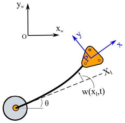
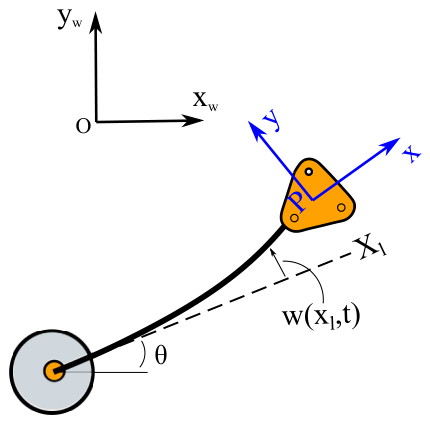
In addition, a camera oCam-5CRO-U with a USB 3.0 interface and CMOS rolling shutter image sensor (Withrobot Inc., Seongnam, Republic of Korea) and a resolution of 640 × 480 pixels, is used to collect in real-time the images of the endpoint of the end-effector. The data is sent to the dSPACE via RS232 protocol at a 60 frames per second (fps) rate. Each image is then processed on a computer, using the software Visual Studio and the proposed algorithm, to calculate the position of the end-effector over the desired movement. The camera is mounted atop the workspace, in an Eye-to-Hand configuration, to capture images of the end-effector. Two reference systems are used to define the movement of the flexible link: the fixed reference frame (defined at the center of the workspace) and the moving reference frame, defined by the center of the colored markers on the end-effector. The center of the workspace is given by , and the moving reference frame is given by . The difference between the center of the workspace and the moving frame estimates the trajectory of the flexible link, including both the rigid and flexible contributions. Figure 3 shows the schematic illustration of the flexible link with the coordinate systems.
Figure 3.
Schematic illustration of the flexible link.
Some steps are required to design the vision-based algorithm. Two colored markers, a red and a green circular marker, are fixed atop the end-effector, as seen in Figure 2, while the green marker is defined by G, the red circular marker is defined by R. The images are processed in both RGB and HSV color spaces, and specific filters are applied to identify the regions of each color. According to the detected marker positions, the proposed algorithm can accurately estimate the mean value of both markers, which define the moving reference frame coordinates. The orientation of the green and red circular markers are, respectively, defined by and . The image processing algorithm uses color filtering techniques based on RGB and HSV color space decomposition, utilizing the OpenCV library. Specific filters identify the red and green regions by assigning binary values to matrix elements depending on pixel color. This allows the algorithm to accurately detect the markers and track the end-effector’s motion throughout the experiment, expressed by P. The end-effector coordinates are then represented by
where correspond to the end-effector linear coordinates, and is the angular orientation. The vision-based method has been previously validated, and additional details can be found in [19].
3. Dynamic Modeling
In this section, we first present the dynamic model of the flexible link based on the decomposition of the link’s rigid-body motion and flexible deformation. Then, due to the limited availability of experimental data, a PINN model is trained using the projected dynamic equation and experimental data in the loss functions.
3.1. Dynamic Model of the Flexible Link
Several mathematical approaches have been proposed in the literature to describe mechanical systems, each characterized by distinct assumptions and levels of complexity. The conventional formulation relies on the Euler–Bernoulli theory, which accounts for bending deformations while neglecting shear effects and rotary inertia. Alternative approaches include the lumped parameter method (LPM), assumed mode method (AMM), and transfer matrix method (TMM) [20,21]. Although these model-based approaches offer several advantages, the computational cost and mathematical complexity represent a limitation for real-time scenarios. In this sense, fast and simple models are an interesting alternative for mechanical systems with fast responses. Several studies conducted at the EESC laboratory have investigated the flexible behavior of flexible manipulators over the years under different trajectories and operating scenarios, allowing the estimation of the most common configurations [19,22]. The dynamics of the flexible link can be expressed as the sum of the rigid base rotation and the flexible deflection along the link (see Figure 3), given by
where is the total displacement at position x along the link at time t, is the rigid-body rotation angle at the base, and is the flexible deformation. Focusing on the principal dynamics observed experimentally, the system is projected onto the modal coordinate , which condenses the total link motion into a second-order ordinary differential equation
where is the angular acceleration of the rigid component, and accounts for the flexibility effects as a function of the strain . As seen, the encoder provides the angular rotation of the link, while the strain gauge estimates its flexible deformation in real time. In this work, is empirically modeled as
where are the parameters to be identified. This phenomenological formulation captures different contributions to the flexible-link dynamics, while keeping the model compact enough for integration into a learning framework. A key motivation for adopting the PINN approach lies in the nature of the available measurements: although strain can be directly measured in real time, acceleration cannot, and estimating it via numerical differentiation would significantly amplify measurement noise, especially in flexible systems. By embedding the governing equations into the network’s loss function, the PINN can infer the unmeasured states, such as acceleration implicitly, without the need for noisy derivative computations.
Furthermore, the parameters are treated as trainable variables in the physics-based loss, making their identification straightforward within the optimization process, as they can be absorbed into the network’s trainable weights and biases. Each term is associated with a different contribution: the linear term is associated with the effective stiffness contribution, while the quadratic term represents amplitude-dependent nonlinearities. The sinusoidal term captures oscillatory nonlinear responses, while the exponential term is strongly related to nonlinear growth or decay characteristics. These features enable the PINN to combine the strengths of data-driven learning with physics-based consistency, providing a practical and efficient way to model the coupled rigid–flexible dynamics. The following subsection details the PINN architecture and training procedure.
3.2. Physics-Informed Neural Networks (PINNs)
Physics-informed neural networks (PINNs) are a network learning strategy that incorporates physical information, typically expressed via constraints derived from differential equations, with data-driven training using observation points or system measurements. This combination encourages the neural network to follow the underlying physical behavior rather than merely fitting the data, enabling the estimation of system states, identification of model parameters, and effective learning even with limited data within the training domain. In practical terms, physics and data are incorporated in the loss function, and the neural network parameters, i.e., weights and biases, are updated via an optimization algorithm.
With this in mind, we briefly recall the structure of a neural network. A neural network is defined by a mathematical model that represents a linear composition of nonlinear functions. This architecture consists of interconnected layers of neurons, with L hidden layers and neurons per layer [23]. Given the input , and the target , the approximated output can be expressed as
where represents the l-th layer transformation
By combining Equations (5) and (6), the relation between the neural network input and the Lth layer is defined by
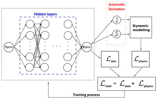
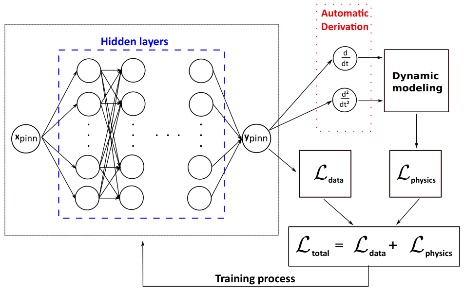
where corresponds to the weights, are the biases of layer, and represents the activation function. In this work, the hyperbolic tangent function is chosen. The set of trainable weights and biases is, respectively, represented by and , which are calculated to minimize the total loss function. The fully connected architecture is depicted in Figure 4.
Figure 4.
Illustration of the proposed PINN considering two loss functions.
In a conventional neural network framework, the difference between the network output and the observed data is used to calculate its loss function. This loss function is designed to minimize the prediction error by employing an appropriate discrepancy metric. Accordingly, the data-driven loss function, denoted as is defined by
where N corresponds to the number of observed data samples.
In the physics-informed context, the loss function includes residual terms corresponding to the governing equations of the mechanical system, in this work, the single flexible link. Assuming the following general ordinary differential Equation (ODE) describing the system,
where represents the differential operator with respect to time, while and correspond, respectively, to the model parameters and external excitation. The ordinary differential equation of second order for the flexible link is defined by Equation (3). The ODE is integrated as part of the loss function to create a learning bias during the training stage. The approximated solution, obtained by a neural network, may satisfy the ODE pointwise. The loss function, referred to as the physics-driven loss function, , is then defined by
where M is the number of the discretization points, also referred to as collocation points, used to evaluate the physics-informed loss. The training dataset consists of eight experimental trajectories, each containing 5000 time samples, resulting in a total of candidate collocation points (such that is the number of trajectories). Automatic differentiation is performed using PyTorch (version 2.13.0), with strain measurements and network outputs normalized for numerical stability while the time variable remains in physical units. Therefore, the total loss function is defined as
where and are weighting coefficients that balance the influence of the loss terms during training steps. Note that the PINN is initially trained using the Python environment (version 3.12) due to its simplicity and the availability of different libraries. Once trained, the algorithm is implemented in the MATLAB/Simulink environment (version 2024) due to the experimental setup.
4. Control Strategy
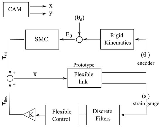
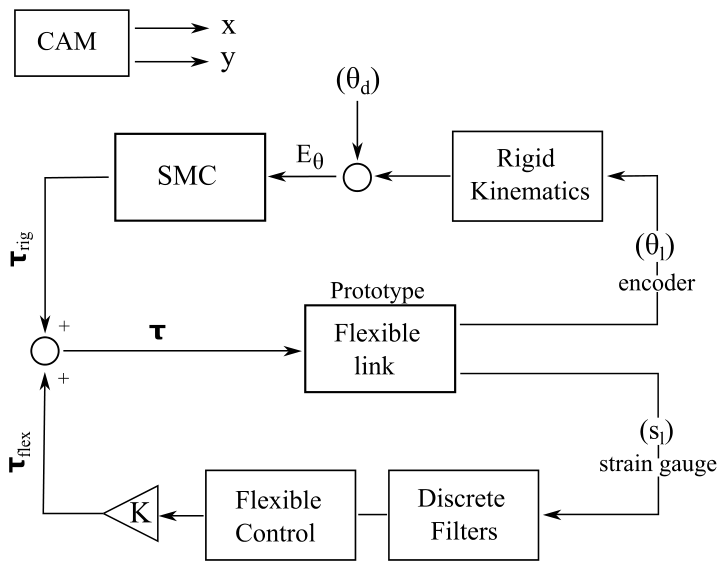
This section is divided into two parts. The first describes the dataset acquisition methodology, whereas the second describes the assessment of the PINN test. The dataset is created by using different rotation angles of the flexible links with an interval of 50 degrees. Figure 5 shows the control scheme used to collect samples for the dataset, which is used for training the PINN.
Figure 5.
Control scheme for constructing a dataset.
The measurement of the encoder () is used to calculate the position of the link, i.e., rigid kinematics. The difference between the rotational angle and the desired angle () is used to calculate the error, as seen by . The sliding mode control (SMC) strategy is designed based on the error and its time derivative [24], while the error is multiplied by the term , its time derivative is also calculated to obtain the sliding surface , as defined by
Note that the final control signal () is formed by the contributions of two loops: one related to the rigid kinematics () and the other to the flexibility (), while the rigid loop is defined by the following expression, , where is a positive gain, the flexible control law is represented by , where the terms K and correspond to the gain and the filtered signal. The sign function is conventionally used to design the SMC; however, since there must be present undesired chattering, a tansig function is chosen to obtain . The signals collected from the strain gauges are passed through discrete filters to reduce noise. The system control law is calculated as the sum of both contributions, as represented by
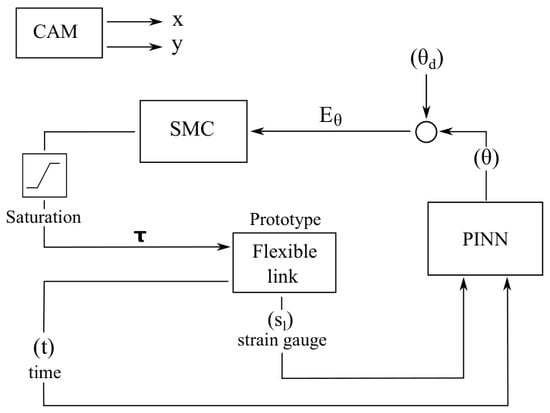
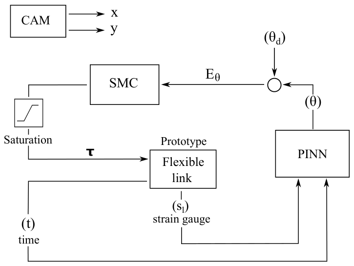
Once the dataset is created by using different trajectories, the PINN strategy is validated. Figure 6 shows the PINN strategy used. As mentioned, two inputs are required to design the PINN: time (t) and strain gauge signal (), while only one output is generated: rotational displacement of the flexible link . Similarly, the SMC strategy uses the error (), calculated by the difference between the rotational displacement obtained via the PINN approach, and the desired angular displacement (), and its time derivative to create the sliding surface. In this case, a single loop is required to design the final control law (), calculated by
which is saturated based on the limitations of the motor. By employing PINN strategy, the camera is used exclusively as an external sensor to estimate the end-effector’s position, i.e., the end-point of the flexible manipulator. The camera operates independently of the proposed control strategy and does not influence its formulation or execution. This endpoint estimation enables the investigation of the total dynamics of the flexible link, including contributions from the rigid kinematics and the flexible characteristics.
Figure 6.
Schematic illustration of the proposed PINN strategy.
5. Results and Discussion
This section evaluates the ability of the PINN to identify the dynamics of the mechanical system. The investigation is performed by evaluating the responses of a flexible robotic manipulator. Firstly, the signals from the strain gauges are collected by using different trajectories. Then, the acquired data are used to train the PINN model and subsequently investigate the PINN strategy, as discussed in Section 4.
5.1. Dataset
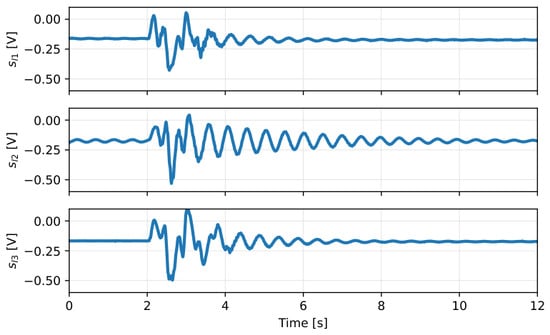
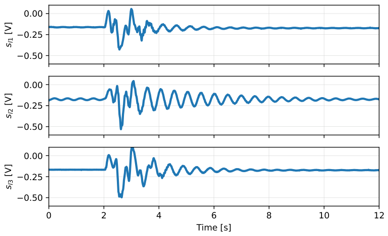
The samples of the dataset are collected using strain gauges on the surface of the flexible link. Based on the trajectory, a different oscillatory behavior is observed. Trajectories were generated using rotation angles ranging from 0.17 rad (10 degrees) to 1.05 rad (60 degrees), covering the experimental workspace. Figure 7 shows representative samples of the strain-gauge signals. The differences in the oscillation time and peaks are mainly related to the proposed trajectory, i.e., larger oscillations of the flexible link produce more pronounced strain-gauge signals. Then, since the inputs of the PINN strategy are formed by the strain-gauge signals and the time, a time vector is created, defined by operational time and the sampling time of the board (dSPACE 1103). The simulation is performed for 12 s and a time step of 0.001 s. After collecting several samples of strain-gauge signals in different scenarios, a dataset is created. The dataset is divided such that 90% is allocated to PINN training, whereas the remaining 10% is used for testing. Note that the data used for the testing phase are unseen samples, i.e., not used during the training and validation phases.
Figure 7.
Samples of the dataset—strain gauge signals.
In addition, based on Figure 5, the control gains used to design the sliding mode control and therefore to conduct the experiments to collect the dataset are defined as , . There is a current saturation of ±1000 mA on the motor due to the company specifications. Further details of the filters and other experimental setups can be found in [22,25].
5.2. PINN Investigation
The PINN investigation is performed by incorporating both the physics-informed terms (see Equation (10)) and the data (see Equation (8)) into the total loss function, as seen in Figure 4. In this study, the training process is performed over 5.000 training steps (represented by epochs). The Adam optimizer [26] is used to update both the neural network parameters and the trainable physical parameters. The proposed PINN architecture consists of five hidden layers, each comprising 40 neurons. Different numbers of hidden layers and neurons are investigated through trial and error to obtain an accurate model. Instead of adopting a fixed learning rate, the OneCycleLR scheduling strategy is used to adaptively modulate the learning rate and momentum throughout training, thereby improving convergence and optimization efficiency. An initial learning rate of is adopted in this work. The OneCycleLR scheduler is applied, with a maximum learning rate of 0.01. To improve stability, gradient clipping is performed with a maximum norm of 1.0. Moreover, the weighting coefficients of the total loss function are defined by trial-and-error, with .
One of the key advantages of using a PINN lies in its ability to estimate unknown parameters directly during the training process. The PINN investigation addresses the main objective of estimating the dynamics of the system and calibrating unknown physical parameters during the training procedure. In this sense, the flexibility of the system is decomposed into different contributions, as shown in Equation (4). Note that the parameters, defined by are, respectively, multiplied by the linear, quadratic, and sinusoidal terms, while is raised to the power of . This strategy is used to investigate the contributions of each term to the total dynamics of the flexible link by assessing the convergence value of each parameter. This approach allows for precise incorporation of flexible dynamics into the kinematic model of a serial manipulator with rigid links.
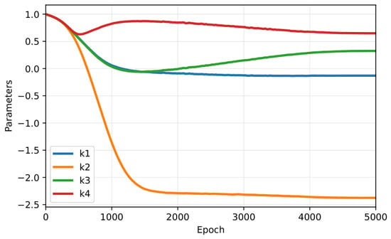
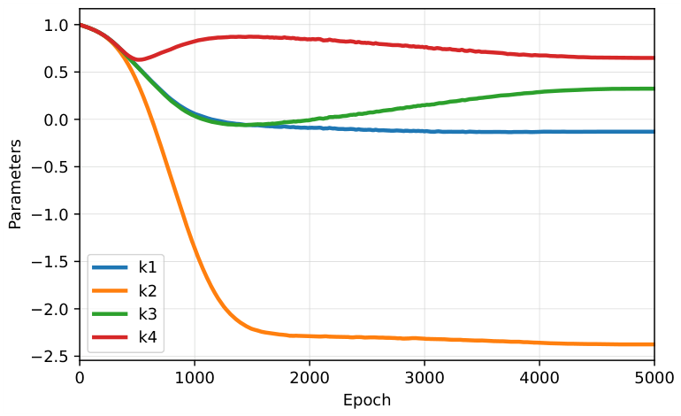
Each parameter is initialized with a value of 1.0, allowing it to adjust freely during training. Moreover, these parameters are not normalized, as they represent phenomenological quantities whose scales are inherently learned by the network. Conversely, the training data, including strain and encoder signals, are mean-centered and scaled by their absolute maximum to improve numerical stability and ensure consistent scaling across different datasets. Figure 8 shows the convergence plots of the equation parameters.
Figure 8.
Convergence plots of the parameters of the flexible effects.
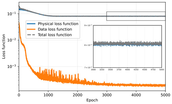
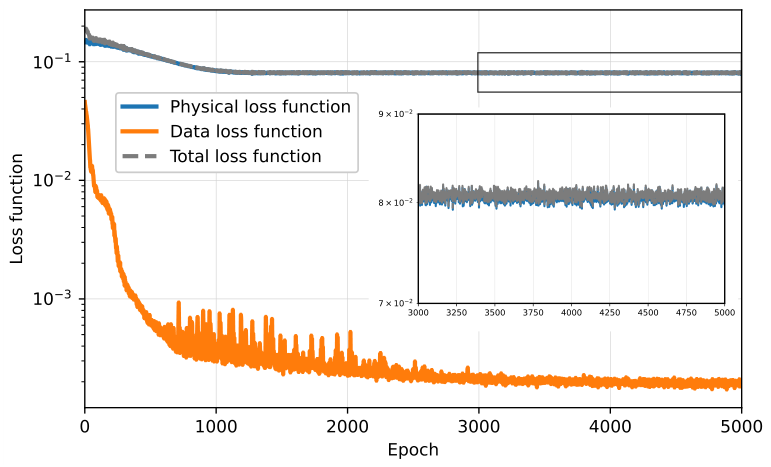
As depicted in Figure 8, convergence is achieved by the linear and quadratic parameters around 1500 epochs, whereas the sinusoidal and exponential terms require approximately 4000 epochs. This difference in convergence behavior may be attributed to the stronger nonlinear nature of the sinusoidal and exponential terms, while the linear and quadratic components are associated with smooth and predictable variations of the input signal, the terms involving sinusoidal and exponential terms are associated with stronger nonlinearities. As a result, the and parameters tend to converge more slowly during training. Moreover, the loss function is observed for the proposed strategy. Figure 9 depicts the evolution of the loss function over the epochs.
Figure 9.
Evolution of the loss functions of the PINN strategy.
As shown in Figure 9, there are two curves: the data loss function, representing the difference between the model predictions and the observed data, and the physical loss function, which enforces the governing physical laws via differential equations. Three main training stages can be identified from the loss curves: an initial phase with high losses due to the network’s early adjustments; a mid-training phase, where both losses decrease significantly as the network learns to fit the data and satisfy the physical constraints; and a final phase, in which the losses plateau, indicating convergence. Therefore, the PINN strategy successfully integrates both observed data and physical laws, leading to a stable and well-converged solution.
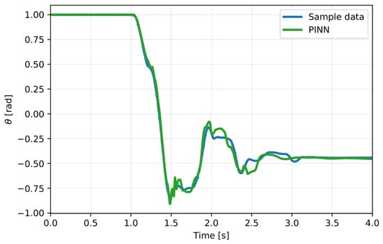
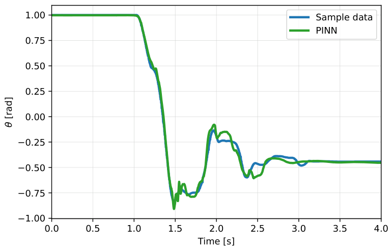
Figure 10 compares the experimental data with the PINN’s output. Despite the experimental test lasting 12 s, the PINN is trained using only four seconds, due to the main characteristics of the encoder’s angle being defined in this time range. After this initial stage, the end-effector reaches its desired position, and no relevant dynamics are observed. The PINN curve accurately follows the sample data, indicating that the PINN strategy has learned to replicate the system’s behavior efficiently. Some slight deviations can be observed in this figure, which can be caused by measurement noise, model assumptions, and the complexity of the physical system. Therefore, the PINN output closely matches the sample data across the time interval, demonstrating the model’s capability to accurately learn and replicate the system dynamics while respecting the underlying physical constraints.
Figure 10.
PINN outputs for the proposed strategy.
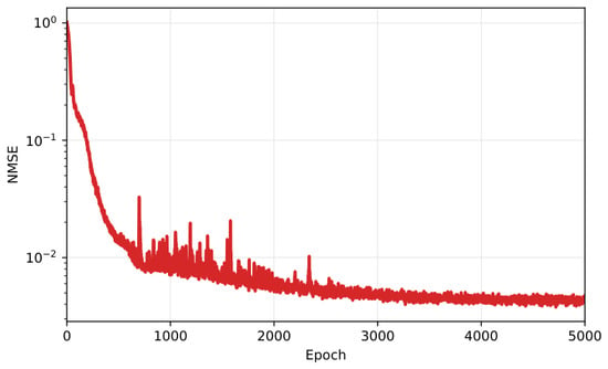
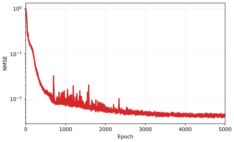
Finally, the Normalized Mean Squared Error (NMSE) metric is used to quantify the accuracy of the predictive model in relation to the variance of the observed data. Note that the closer the NMSE value is to zero, the better the prediction. Figure 11 shows the NMSE value for the PINN investigation. The metric reaches nominal values closer to zero after a few iterations, as seen by the 500 epochs, which indicates that the PINN effectively captures the system dynamics. This result shows similar characteristics to those of the loss functions, as seen in Figure 9.
Figure 11.
Normalized Mean Squared Error over Training Epochs.
5.3. Closed-Loop Experimental Validation
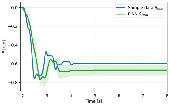
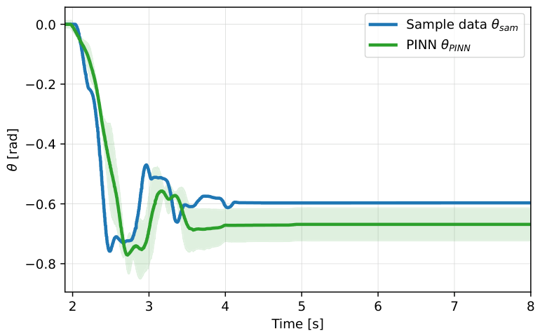
The proposed strategy is validated experimentally, as seen in Figure 6. Several experimental trials are performed to investigate the PINN efficiency. An average of these experimental runs is computed to illustrate the characteristic behavior of the analyzed signals. Moreover, to assess the variability and statistical reliability of the predicted outputs, a 90% confidence interval (CI) is calculated over the experimental trials, since the experiment was repeated several times to assess the performance of the proposed strategy. At each time step, the CI is estimated by the mean ± margin of error, which is defined by the product of the standard error of the mean (SEM) and the critical value of the t-distribution corresponding to a 90% confidence level. This approach enables a quantitative measure of uncertainty and allows a visual comparison of the prediction consistency of datasets. Similar to the PINN validation (see Section 5.2), the analyzed time is lower than 12 s, ranging from 1.9 to 8 s. This procedure is adopted to remove the stationary state and highlight the main characteristics of the desired motion. Figure 12 shows the experimental comparison between the results obtained by the PINN strategy and those calculated by the encoder.
Figure 12.
Closed-loop experimental comparison of encoder measurements from sample data and PINN output.
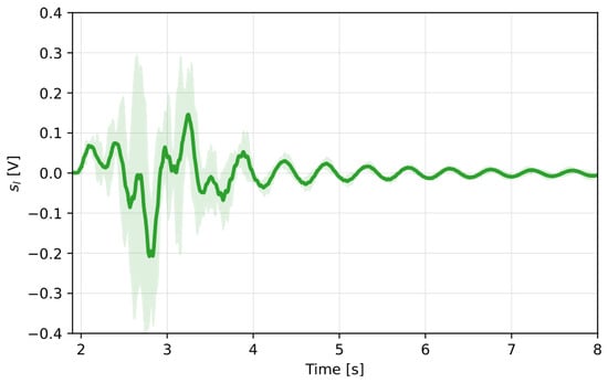
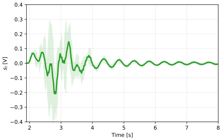
Similar to the PINN results, the closed-loop experimental validation shows agreement with the proposed method. As illustrated in Figure 12, the signal estimated by the PINN exhibits behavior closely aligned with the encoder measurements. Moreover, the confidence interval confirms that all experimental trials exhibit consistent behavior, reinforcing the reliability and validity of the proposed approach under experimental conditions. The strain-gauge signals are also evaluated. Similar to the encoder measurements, the results show high reproducibility within the confidence interval, demonstrating the positive results of the strain gauge estimation. Figure 13 shows the mean representation of the strain gauge signals in the presence of the PINN strategy.
Figure 13.
Closed-loop experimental investigation of the strain gauge signals using PINN strategy.
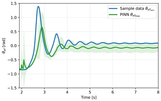
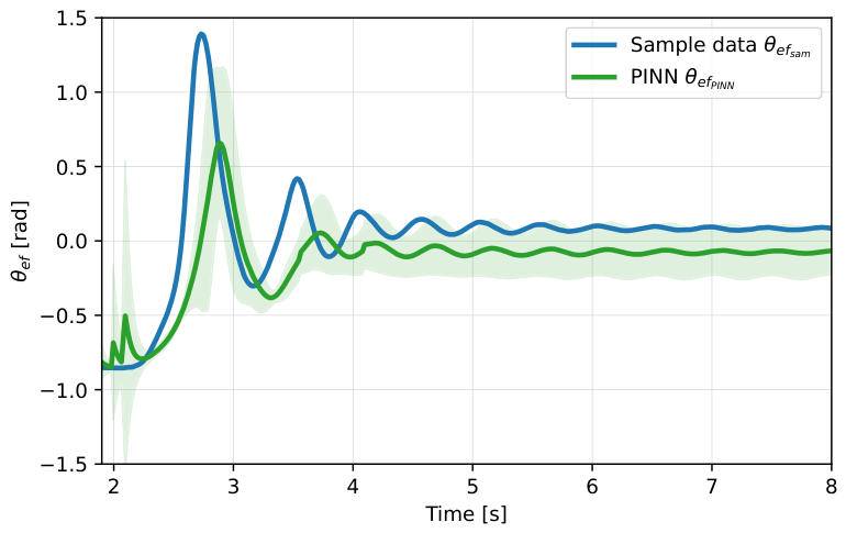
The camera is used to estimate the end-effector position and also to assess the proposed strategy. Figure 14 shows the end-effector position over two cases: data sample and PINN strategy. The end-effector position estimated by the PINN closely matches the reference signal across the entire time interval. This agreement highlights the model’s ability to accurately reconstruct the system output, further supporting the reliability of the proposed method in capturing the dynamic behavior of the end-effector. In addition, similar to Figure 12, the confidence interval indicates that the characteristics of the flexible link are estimated adequately.
Figure 14.
Closed-loop experimental comparison of end-effector measurements from sample data and PINN output.
The root mean square (RMS) methodology is also employed to investigate the performance of the proposed strategy. RMS is calculated as , where N is the length of the vector and is the error of each variable at j instant of time. The errors, between the desired (sample data) and calculated values (PINN), obtained from both the encoder (see Figure 12) and end-effector measurements (see Figure 14) are calculated to estimate their nominal magnitudes. Based on the RMS equation, the nominal values obtained from the encoder and end-effector are, respectively, 0.076 and 0.233. The encoder shows a lower RMS value, as it is mainly influenced by rigid-body kinematics, which reduces uncertainties and model complexity. In contrast, the end-effector shows a higher RMS value due to the additional uncertainties introduced by link flexibility. Therefore, the significant increase in RMS values highlights one of the main contributions of this paper: the use of PINNs to compensate for uncertainties and flexibility effects within the rigid-body kinematics framework.
6. Final Remarks
Robotic manipulators are widely used to perform tasks that are hazardous, repetitive, and labor-intensive. They are typically designed with rigid links to suppress end-effector vibrations and enhance positional accuracy. However, the increased mass and inertia of rigid-link manipulators can reduce energy efficiency and limit dynamic performance relative to the payload capacity. In this context, lightweight flexible-link manipulators have gained attention in recent years due to their advantages, including reduced cost, higher speed, higher payload-to-weight ratios, smaller actuators, and enhanced maneuverability. Nevertheless, the primary limitation of such flexible systems lies in their lightweight structure, which can lead to undesirable vibrations, complex dynamic modeling, and significant challenges in designing effective control strategies.
This study assesses the development and validation of a PINN to estimate the dynamic behavior of a flexible-link manipulator. The experimental setup consists of a single flexible stainless steel link actuated by a brushless DC motor, with real-time measurements collected using an encoder and strain gauges. The strain gauges are used to measure the link oscillations, while the encoder is used to measure the rotational angle of the flexible link. Moreover, a camera tracks the end-effector position using a custom image processing algorithm. A dataset is created by executing different trajectories under closed-loop control. Based on the dataset, the PINN is then trained using time and strain signals as inputs to estimate the angular displacement, combining a data-driven loss with a physics-based loss derived from the system’s dynamic model. The trained model is evaluated in a closed-loop configuration to verify its ability to learn and generalize the system’s nonlinear behavior with high accuracy.
The results show that the PINN effectively integrates experimental data with physical constraints, achieving accurate predictions of link dynamics. The PINN outputs exhibit close agreement with the sampled data throughout the evaluated time interval, thereby demonstrating the model’s capability to learn and replicate the system dynamics. Likewise, the experimental results show strong consistency with the proposed method, as shown by the comparison with encoder and end-effector responses. Moreover, the confidence interval confirms that all experimental trials present consistent behavior, supporting the reliability and validity of the proposed approach under experimental conditions. Consequently, the proposed strategy demonstrates accuracy and reliability in capturing the flexible dynamics of the serial manipulator.
Future work includes using the proposed PINN as a generalized model for flexible robotic manipulators with different materials, thicknesses, and other properties. Additional investigations should investigate payload variation, stiffness-to-mass ratio, damping, geometry, strain-gauge location, controller gains, and external disturbances, while distinguishing among zero-shot transfer, fine-tuning, and complete retraining. Comparisons among a neural network, a conventional nonlinear observer, and reduced PINN variants containing different subsets can also be addressed. Moreover, comparisons with conventional estimation methods and data-driven neural networks can be investigated, together with ablation studies to quantify the contribution of the physics-informed loss. Formal stability analyses and robustness evaluations under uncertainties and varying operating conditions can also be addressed.
Author Contributions
Conceptualization, T.J.T., R.S.G., R.d.O.T. and M.M.d.S.; methodology, T.J.T., R.d.O.T. and M.M.d.S.; validation, T.J.T., R.S.G., R.d.O.T. and M.M.d.S.; formal analysis, T.J.T., R.S.G., R.d.O.T. and M.M.d.S.; investigation, T.J.T., R.S.G., R.d.O.T. and M.M.d.S.; writing—original draft preparation, T.J.T. and R.S.G.; writing—review and editing, R.d.O.T. and M.M.d.S.; supervision, R.d.O.T. and M.M.d.S. All authors have read and agreed to the published version of the manuscript.
Funding
This work was supported by the São Paulo Research Foundation—FAPESP [grant numbers 18/21336-0, 23/07834-6 and 24/07967-9], and the National Council for Scientific and Technological Development—CNPq [grant number 303884/2021-5].
Data Availability Statement
The original contributions presented in this study are included in the article. Further inquiries can be directed to the corresponding author.
Conflicts of Interest
The authors declare no conflicts of interest.
Abbreviations
The following abbreviations are used in this manuscript:
| PINN | Physics-Informed Neural Network |
| PDEs | Partial Differential Equations |
| FEM | Finite Element Model |
| TSMC | Terminal Sliding Mode Control |
| LPM | Lumped Parameter Method |
| AMM | Assumed Mode Method |
| TMM | Transfer Matrix Method |
| SMC | Sliding Mode Control |
| CI | Confidence Interval |
| SEM | Standard Error of the Mean |
| RMS | Root Mean Square |
References
- Sayahkarajy, M.; Mohamed, Z.; Mohd Faudzi, A.A. Review of modelling and control of flexible-link manipulators. Proc. Inst. Mech. Eng. Part I J. Syst. Control Eng. 2016, 230, 861–873. [Google Scholar] [CrossRef] [Scilit]
- Bilal, H.; Aslam, M.S.; Tian, Y.; Yahya, A.; Abu Izneid, B. Enhancing trajectory tracking and vibration control of flexible robots with hybrid fuzzy ADRC and input shaping. IEEE Access 2024, 12, 150574–150591. [Google Scholar] [CrossRef] [Scilit]
- Subudhi, B.; Morris, A.S. Dynamic modelling, simulation and control of a manipulator with flexible links and joints. Robot. Auton. Syst. 2002, 41, 257–270. [Google Scholar] [CrossRef] [Scilit]
- Dehkordi, S.F. Dynamic analysis of flexible-link manipulator in underwater applications using Gibbs–Appell formulations. Ocean Eng. 2021, 241, 110057. [Google Scholar] [CrossRef] [Scilit]
- Berger, T.; Drücker, S.; Lanza, L.; Reis, T.; Seifried, R. Tracking control for underactuated non-minimum phase multibody systems. Nonlinear Dyn. 2021, 104, 3671–3699. [Google Scholar] [CrossRef] [Scilit]
- Li, B.; Li, X.; Gao, H.; Wang, F.Y. Advances in flexible robotic manipulator systems—Part I: Overview and dynamics modeling methods. IEEE/ASME Trans. Mechatron. 2024, 29, 1100–1110. [Google Scholar] [CrossRef] [Scilit]
- Ji, N.; Liu, Z.; Liu, J.; He, W. Vibration control for a nonlinear three-dimensional Euler–Bernoulli beam under input magnitude and rate constraints. Nonlinear Dyn. 2018, 91, 2551–2570. [Google Scholar] [CrossRef] [Scilit]
- Hwang, Y.L. Recursive Newton–Euler formulation for flexible dynamic manufacturing analysis of open-loop robotic systems. Int. J. Adv. Manuf. Technol. 2006, 29, 598–604. [Google Scholar] [CrossRef] [Scilit]
- Mishra, N.; Singh, S.P. Determination of modes of vibration for accurate modelling of the flexibility effects on dynamics of a two-link flexible manipulator. Int. J. Non-Linear Mech. 2022, 141, 103943. [Google Scholar] [CrossRef] [Scilit]
- Garpelli, L.N.; Alves, D.S.; Cavalca, K.L.; de Castro, H.F. Physics-guided neural networks applied in rotor unbalance problems. Struct. Health Monit. 2023, 22, 4117–4130. [Google Scholar] [CrossRef] [Scilit]
- Bao, Y.; Thesma, V.; Mohammadpour Velni, J. Physics-Guided and Neural Network Learning-Based Sliding Mode Control. IFAC-PapersOnLine 2021, 54, 705–710. [Google Scholar] [CrossRef] [Scilit]
- Yang, X.; Zhou, Z.; Li, L.; Zhang, X. Collaborative Robot Dynamics with Physical Human–Robot Interaction and Parameter Identification with PINN. Mech. Mach. Theory 2023, 189, 105439. [Google Scholar] [CrossRef] [Scilit]
- Wang, X.; Dabrowski, J.J.; Pinskier, J.; Liow, L.; Viswanathan, V.; Scalzo, R.; Howard, D. PINN-ray: A physics-informed neural network to model soft robotic fin ray fingers. In IEEE/RSJ International Conference on Intelligent Robots and Systems (IROS); IEEE: New York, NY, USA, 2024; pp. 247–254. [Google Scholar]
- Soyleyici, C.; Unver, H.O. A Physics-Informed Deep Neural Network Based Beam Vibration Framework for Simulation and Parameter Identification. Eng. Appl. Artif. Intell. 2025, 141, 109804. [Google Scholar]
- Li, T.; Xiao, T. Physics-informed neural network-based input shaping for vibration suppression of flexible single-link robots. Actuators 2025, 14, 14. [Google Scholar] [CrossRef] [Scilit]
- Li, Z.; Wu, S.; Chen, W.; Sun, F. Physics-informed neural networks for compliant robotic manipulators dynamic modeling. J. Comput. Sci. 2025, 90, 102633. [Google Scholar] [CrossRef] [Scilit]
- Savio, T.L.; Geronel, R.S.; da Silva, M.M. Dynamic modeling of a novel catamaran robotic system actuated by bio-inspired propulsion devices using physics-informed neural networks. Ocean Eng. 2025, 326, 120806. [Google Scholar] [CrossRef] [Scilit]
- Kan, Y.; Xue, D.; Liu, H.; Liu, X. Sliding-mode vibration control of flexible structures via physics-informed neural network-based modeling. In Joint International Conference on Automation-Intelligence-Safety (ICAIS) and International Symposium on Autonomous Systems (ISAS); IEEE: New York, NY, USA, 2025; pp. 1–7. [Google Scholar]
- da Silva, M.M.; Colombo, F.T.; de Oliveira, G.C.; de Oliveira, L.P.R. Hybrid vision/strain-based control strategy for a parallel manipulator with flexible links. Mech. Mach. Theory 2024, 191, 105508. [Google Scholar] [CrossRef] [Scilit]
- Lochan, K.; Roy, B.K.; Subudhi, B. A review on two-link flexible manipulators. Annu. Rev. Control 2016, 42, 346–367. [Google Scholar] [CrossRef] [Scilit]
- Garcia-Perez, O.A.; Silva-Navarro, G.; Peza-Solis, J.F. Flexible-link robots with combined trajectory tracking and vibration control. Appl. Math. Model. 2019, 70, 285–298. [Google Scholar] [CrossRef] [Scilit]
- Geronel, R.S.; Santos, J.C.; da Silva, M.M. Executable digital twin for a flexible robotic link. J. Braz. Soc. Mech. Sci. Eng. 2025, 47, 600. [Google Scholar] [CrossRef] [Scilit]
- Teloli, R.D.O.; Tittarelli, R.; Bigot, M.; Coelho, L.; Ramasso, E.; Le Moal, P.; Ouisse, M. A physics-informed neural networks framework for model parameter identification of beam-like structures. Mech. Syst. Signal Process. 2025, 224, 112189. [Google Scholar] [CrossRef] [Scilit]
- Slotine, J.J.E.; Li, W. Applied Nonlinear Control; Prentice-Hall: Englewood Cliffs, NJ, USA, 1991. [Google Scholar]
- Geronel, R.S.; Oliveira, G.C.; Silva, M.M. Dual-loop control strategies for vibration attenuation of a flexible parallel manipulator. J. Vib. Control 2024, 32, 1007–1019. [Google Scholar] [CrossRef] [Scilit]
- Zhang, Z. Improved Adam optimizer for deep neural networks. In IEEE/ACM 26th International Symposium on Quality of Service (IWQoS); IEEE: New York, NY, USA, 2018; pp. 1–2. [Google Scholar]
Disclaimer/Publisher’s Note: The statements, opinions and data contained in all publications are solely those of the individual author(s) and contributor(s) and not of MDPI and/or the editor(s). MDPI and/or the editor(s) disclaim responsibility for any injury to people or property resulting from any ideas, methods, instructions or products referred to in the content. |
© 2026 by the authors. Licensee MDPI, Basel, Switzerland. This article is an open access article distributed under the terms and conditions of the Creative Commons Attribution (CC BY) license.