Adaptive Adjustment of Advantage Estimation for Robot Control Using Reinforcement Learning

Abstract

In robotics control experiments, the balance between exploration and exploitation, as well as the accuracy of the advantage function estimation, are crucial factors that affect the effectiveness of policy optimization methods. To overcome these challenges, this paper proposes an adaptive adjustment of advantage estimation based on the policy loss and policy entropy algorithm (A3E-PLE), which can improve the exploratory capabilities of the proximal policy optimization (PPO) algorithm. Specifically, on the one hand, the policy loss is adjusted using a Gaussian distribution policy entropy to mitigate randomness and separate policy improvement from random noise, thereby improving exploration efficiency. On the other hand, to adapt flexibly to various training scenarios and further enhance the accuracy of advantage function estimation, the policy loss is incorporated into the advantage function estimation. This enables the algorithm to adaptively adjust according to changes in the strategy. Finally, the proposed reinforcement learning (RL) framework was validated using robot control simulations and complex decision-making environments. It is shown that A3E-PLE achieves higher learning efficiency and greater rewards compared to traditional generalized advantage estimation.

1. Introduction

Robotics is an interdisciplinary field that integrates artificial intelligence, automatic control, sensing technology, and computer science. In this field, robot control tasks are a core component of robotics technology, enabling robots to autonomously perceive their environment, make decisions, and take action [1]. From early path planning algorithms to modern intelligent obstacle avoidance [2], autonomous navigation [3,4], and human–robot interaction [5], robot control technologies have advanced substantially. However, achieving efficient robot motion control in complex decision-making environments remains a formidable challenge. During robot movement, robots need to autonomously perceive the surrounding environment and adjust their movement strategies according to environmental information. Especially in dynamically changing environments, robust perception, decision-making capabilities, and advanced control algorithms are required to adjust the robot’s motion more quickly and accurately. Traditional robot control algorithms include the Proportional–Integral–Derivative (PID) control [6], sliding mode control [7], and fuzzy control [8]. Nevertheless, these methods depend on the accuracy of the fixed model and parameters, making it difficult to adapt to robot control in complex and changeable environments [9].

Driven by advances in deep learning and reinforcement learning, data-driven control approaches have enabled more adaptive and robust robotic systems, improving their performance in complex and uncertain environments. These enhancements have enabled robots to play a crucial role in many fields. Reinforcement learning aims to learn an optimal policy to maximize rewards through interaction with the environment [10]. Therefore, the primary goal of reinforcement learning is to improve policies, which can generally be categorized into two types of methods. Value-based optimization methods, such as Q-Learning [11] and DQN [12], evaluate the long-term expected return of each action in a given state by optimizing an action-value function. Based on the aforementioned assessment, the optimal action is further determined. The other is Policy-Based Optimization methods, including Policy Gradient algorithms [13], Trust Region Policy Optimization [14], and Proximal Policy Optimization (PPO) [15]. These methods directly optimize the policy and update the policy parameters by computing the policy gradient to maximize expected return. Among them, the PPO algorithm ensures the stability of policy updates by imposing constraints on the step size of the update. This stability enhances learning efficiency and policy quality, leading to improved performance in continuous control tasks.

However, policy gradient methods often exhibit high variance, which may lead to learning instability or overfitting [16]. To overcome these problems, some researchers have introduced the advantage function to construct the policy gradient. The advantage function denotes the disparity between the Q-value and the average value of all possible actions in that state. Thus, an accurate estimation of the advantage function is crucial for the performance of policy gradient methods and Actor–Critic architectures. As a fundamental method utilizing advantage functions, the Asynchronous Advantage Actor–Critic (A3C) approach operates on fixed-length experience segments (e.g., 20 time steps), which are used to compute discounted returns and advantage estimates for asynchronous parameter updates [17]. The implementation of A3C by OpenAI demonstrates that the synchronous, deterministic version, known as Advantage Actor–Critic [18], outperforms the asynchronous variant and better utilizes GPUs. Nonetheless, since advantage estimation is typically influenced by a variety of factors, including data sparsity, model bias, and parameter sensitivity, the resulting estimation errors will ultimately impede the effectiveness of policy learning and reduce sample efficiency.

In recent years, extensive studies have been devoted to reducing value function estimation errors through improved data utilization and optimized network architectures. For instance, Generalized Advantage Estimation (GAE) incorporates Temporal Difference (TD) residuals and adjusts the $\lambda$ parameter to balance the current state value and future returns, thereby seeking the optimal balance between short-term and long-term benefits [19]. Direct Advantage Estimation [20] establishes an advantage function model that is independent of the action-value function from the policy trajectory, thereby minimizing error accumulation and enhancing estimation accuracy. To address the exploration–exploitation dilemma, Park et al. [21] employed multi-modal advantage functions to approximate the true advantage and achieve more accurate results with more comprehensive experience. Following their work [21], Zhang et al. [22] introduced a learnable explorer to reduce overestimation and seek a better policy while studying the effect of action selection strategies on estimation biases. In addition, the sensitivity of the advantage function parameters can also cause misjudgment of advantage-maximizing actions, reducing sample efficiency. To overcome these difficulties, Zhang et al. [23] introduced independent advantage estimation to reduce estimation variance by identifying independence between current actions and future states when learning a reward decomposition model. To further balance bias and variance in estimating advantages, Chen et al. [24] proposed an adaptive method to optimize the combination of state values and sample returns by adjusting the weight parameter $\lambda$.

Moreover, the choice of the discount factor $\gamma$ has an important impact on the accuracy and sample efficiency of the advantage function estimation. The selection of an appropriate $\gamma$ may vary from task to task and usually requires experience and debugging. In practice, the value of $\gamma$ needs to be adjusted according to the characteristics of the specific problem and algorithm. It is common practice to use Exponential Discounting ${\gamma }^t$, assigning a constant value to the discount factor while propagating it exponentially. Illustratively, in the PPO algorithm, $\gamma$ is often set to 0.99, signifying that the agent weighs long-term rewards more heavily when making decisions. Naik et al. [25] showed that maximizing the objective function of discounted reinforcement learning is not equivalent to finding an optimal policy in a continuous task. The introduced discounting mechanism results in long-term return decaying exponentially, making it complex and challenging to optimize the policy directly with traditional methods. Alexander et al. [26] conducted a study exploring the connection between hyperbolic discount factors and exponentially discounted future rewards. Their findings revealed that within the classical framework of monotonically decreasing exponential rewards, agents struggled to fully capitalize on rewards spanning a broad range. Zinzuvadiya et al. [27] optimized learning processes by dynamically adjusting the discount factor. Their method employed empirical observations of state values encountered during episodic trajectories to iteratively refine state-specific discount rates. The algorithm, based on state-dependent discount factors, relies on retaining the observation sequence and is not suitable for application in Deep Reinforcement Learning (DRL). François-Lavet et al. [28] experimentally demonstrated that gradually incrementing the discount factor to its final value led to a marked reduction in learning steps, thereby enhancing learning efficiency. The dynamic discount factor policy introduced in their study outperformed the conventional DQN method across multiple experiments.

To address the issues discussed above, this paper proposes a novel algorithm named “A3E-PLE”, which improves advantage estimation through adaptive adjustment based on real-time feedback from policy changes. Specifically, we introduce the concept of policy entropy into the algorithm and adjust it using a Gaussian distribution. This involves incorporating entropy into the loss function to harmonize the objectives of maximizing rewards and encouraging exploration. In this manner, all agents are encouraged to explore new actions and uncover potential optimal strategies. Subsequently, we leverage policy loss as a feedback signal to dynamically update the discount factor, which addresses the limitation of fixed discounting in conventional advantage estimation. It should be noted that the algorithm proposed in this paper can adaptively adjust to policy changes, thereby further enhancing the accuracy of the advantage function estimation. Finally, using the PPO algorithm, we conducted extensive experimental evaluations across various simulated robot control environments.

The contributions of this paper are summarized as follows:

(1) Employing a policy entropy based on the Gaussian distribution to adjust policy loss reduces randomness and enhances exploration efficiency.

(2) Introducing policy loss to dynamically update the discount factor $\gamma$, thereby strengthening the connection between policy gradients and advantages.

(3) Adjusting policy Loss through policy entropy to indirectly improve the advantage estimation.

The remainder of this paper is structured as follows. Section 2 introduces the fundamental background of the advantage function. Section 3 provides a detailed explanation of the principles and implementation details of the A3E-PLE algorithm. In Section 4, experiments are conducted using standard control environments from OpenAI Gym and adversarial environments provided by ML-Agents to validate the effectiveness of the proposed method. Finally, Section 5 presents the conclusions, including a thorough analysis of the experimental results and a discussion on the potential applications of the A3E-PLE algorithm in the study of robot motion control strategies.

Notation Nomenclature

Table 1 summarizes the mathematical notations, model parameters, and hyperparameters used throughout the study for quick reference.

Table 1. Summary of Mathematical Notations.

Symbol	Definition
$\theta$	Policy network learnable parameters
$\varphi$	Value network learnable parameters
$\lambda$	GAE bias–variance trade-off coefficient
$ϵ$	PPO clip threshold coefficient
$\alpha$	Policy entropy coefficient
$\gamma$	Reward discount factor
$\beta$	Step size for adaptive $\gamma$ update
$\eta$	Gradient descent learning rate
$\mu$	Smoothing factor
$s_t,a_t,r_t$	State, action and reward at time step t

2. Background

2.1. Policy Gradient

Reinforcement learning (RL) tasks involve continuous decision-making interactions between an agent and its environment. In this context, a policy represented by $\pi$ associates each state $s_t$ in the state space S with an action $a_t$ in the action space A at a given time step t. Policy gradient is a canonical policy-based reinforcement learning method. It parameterizes the policy function and optimizes these parameters to maximize the expected return. Inspired by gradient ascent methods [19], this paper estimates the advantage of the improved policy to enhance the policy.

The expression can be expressed as follows:

$$\begin{array}{c}\hfill g^{\gamma }:={\mathbb{E}}_{\begin{array}{c}{s}_{0:\infty }\\ a_{0:\infty }\end{array}}\left[{\sum }_{t=0}^{\infty }{A}^{\pi ,\gamma }(s_t,a_t){▽}_{\theta }log{\pi }_{\theta }\left(a_t\right|s_t)\right]\end{array}$$

(1)

where $A^{\pi ,\gamma }\left(s_t,a_t\right)$ represents the Advantage Function at state $s_t$ when action $a_t$ is taken. It indicates the advantage of taking action $a_t$ relative to the average performance in the current state. ${\nabla }_{\theta }\log {\pi }_{\theta }\left(a_t\mid s_t\right)$ represents the gradient of the logarithm of the policy ${\pi }_{\theta }$ with respect to the parameters $\theta$. It signifies the gradient of the logarithm of the probability of selecting action $a_t$ given state $s_t$ under the current parameter $\theta$. The discounted return $g^{\gamma }$ represents the cumulative expected return starting from the initial state under the current policy $\pi$ with the discount factor $\gamma$.

The goal of the policy gradient approach is to identify a policy that maximizes the expected return through interaction between the agent and the environment. Given the complexity and computational cost of directly maximizing the expected return, an indirect strategy is employed. This involves defining a loss function that is closely related to the expected return and then minimizing it. A standard practice is to define a loss function as the negative expected return, such that minimizing the loss is equivalent to maximizing the return.

In general, the policy loss is undefined because the policy gradient method does not depend on a loss function to directly optimize policy parameters. However, when neural networks are used to model the policy, a loss function becomes a necessary condition for backpropagation and optimization. Therefore, the loss function in this paper is defined as follows:

$$\begin{array}{c}\hfill L^{\mathrm{CLIP}}\left(\theta \right)=-E_t\left[min(r_t\left(\theta \right)·A_t,clip(r_t\left(\theta \right),1-ϵ,1+ϵ)·A_t)\right]\end{array}$$

(2)

where $clip(x,a,b)$ is a function that clips the value x to lie within the interval $[a,b]$. $ϵ$ is a hyperparameter that controls the range of clipping. $\left[r_t\left(\theta \right):={\displaystyle \frac{{\pi }_{\theta }\left(a_t\right|s_t)}{{\pi }_{{\theta }_{old}}\left(a_t\right|s_t)}}\right]$ is the ratio of action probabilities under the current policy ${\pi }_{\theta }$ to the old policy ${\pi }_{{\theta }_{old}}$.

Note that the policy loss $L^{\mathrm{CLIP}}\left(\theta \right)$ derived by averaging the individual losses at time step t in Equation (2) is used to represent the expectation of the loss minimization at the current policy parameter $\theta$. It is treated as the negative loss function in policy gradient methods, aiming to maximize the expected return by minimizing this negative loss function. Subsequently, gradients of this loss function are computed with respect to the model’s parameters, namely, the weights and biases of the policy network. This approach promotes an update of the policy in a direction that favors higher returns.

2.2. Advantage Function

The advantage function plays a crucial role in reinforcement learning, serving as a metric that evaluates the relative merits of executing a given action in a specified state compared to the current policy [29]. Its primary purpose is to optimize the policy, helping the agent to discern which actions are advantageous under the present circumstances. In the context of Policy Gradient methods, the advantage function is frequently used to guide policy updates. By optimizing the probabilities of actions with high advantage values, agents can learn efficient policies more effectively. The advantage function $A^{\pi ,\gamma }(s_t,a_t)$ can be expressed as follows:

$$\begin{array}{c}\hfill Q^{\pi ,\gamma }(s_t,a_t):={\mathbb{E}}_{\begin{array}{c}t+1:\infty \\ a_{t+1:\infty }\end{array}}\left[{\sum }_{l=0}^{\infty }{\gamma }^l{r}_{t+l}\right]\end{array}$$

(3)

$$\begin{array}{c}\hfill V^{\pi ,\gamma }\left(s_t\right):={\mathbb{E}}_{\begin{array}{c}t+1:\infty \\ a_{0:\infty }\end{array}}\left[{\sum }_{l=0}^{\infty }{\gamma }^l{r}_{t+l}\right]\end{array}$$

(4)

$$\begin{array}{c}\hfill A^{\pi ,\gamma }(s_t,a_t):=Q^{\pi ,\gamma }(s_t,a_t)-V^{\pi ,\gamma }\left(s_t\right)\end{array}$$

(5)

where $Q^{\pi ,\gamma }\left(s_t,a_t\right)$ in Equation (3) represents the expected return of taking action $a_t$ in state $s_t$, and $V^{\pi ,\gamma }\left(s_t\right)$ in Equation (4) denotes the expected return under the current policy in state $s_t$.

The estimation of the advantage function can be achieved using value function prediction techniques, specifically Monte Carlo (MC) methods [30] and Temporal Difference (TD) methods [31]. MC methods operate without a complete understanding of the environment, they rely solely on past interactions. Being model-free and empirical in nature, MC methods provide unbiased evaluations of state values. However, they require experiences spanning entire episodes to ascertain value functions, resulting in significant variance. In contrast, TD methods combine concepts from dynamic programming and MC methodologies. They refine value functions by leveraging single-step discrepancies at each time step, thus reducing variance while potentially introducing a higher level of bias. The TD error formula is given in Equation (6):

$$\begin{array}{c}\hfill {\delta }_t=r_t+\gamma V\left(s_{t+1}\right)-V\left(s_t\right)\end{array}$$

(6)

where ${\delta }_t$ is the TD error at the time step t. $r_t$ is the reward. $\gamma$ is the discount factor. $V\left(s_{t+1}\right)$ is the state-value function of the next state $s_{t+1}$. $V\left(s_t\right)$ is the state value function of the current state $s_t$.

The current advantage corresponds to the anticipated TD error at the subsequent time step. However, this advantage remains unbiased only when the estimation is accurate. The $\lambda$-return algorithm [32], which averages state value estimates, integrates TD and MC methodologies, achieving a balance between bias and variance. Nonetheless, its computation requires sampling an entire episode. The advantage function is shown in Equation (7):

$$\begin{array}{c}\hfill {\widehat{A}}_t^{(\infty )}:={\displaystyle \sum _{l=0}^{\infty }}{\gamma }^l{\delta }_{t+l}^V=-V\left(s_t\right)+{\displaystyle \sum _{l=0}^{\infty }}{\gamma }^l{r}_{t+l}\end{array}$$

(7)

In the Generalized Advantage Estimation (GAE) [19] framework, the discount factor $\gamma$ serves as the core parameter governing long-term return trade-offs, while $\lambda$ functions as an auxiliary parameter controlling estimation bias. This study prioritizes optimization of $\gamma$ and employs a standard $\lambda =0.95$ to maintain benchmark comparability. The foundational GAE formulation is expressed in Equation (8):

$$\begin{array}{c}\hfill {\widehat{A}}_t^{(\pi ,\gamma )}:={\displaystyle \sum _{l=0}^{\infty }}{\left(\gamma \lambda \right)}^l{\delta }_{t+l}^V\end{array}$$

(8)

Here, $\gamma$ determines the decay rate of future rewards, and $\lambda \in [0,1]$ regulates the bias–variance trade-off in advantage estimation. These parameters operate synergistically: $\gamma$ governs temporal discounting of absolute rewards, while $\lambda$ manages credit assignment for relative advantage. At extreme values of $\lambda$, the estimator simplifies to temporal difference (TD) or Monte Carlo (MC) methods, as shown in Equations (9) and (10): where $\gamma$ is the discount factor controlling long-term reward decay, and $\lambda \in [0,1]$ is the “bias–variance trade-off parameter” for advantage estimation. Among them, $\gamma$ directly determines the decay rate of future rewards. This dual-parameter system operates as:

$$\begin{array}{c}\hfill GAE(\gamma ,0):{\widehat{A}}_t:={\delta }_t=r_t+\gamma V\left(s_{t+1}\right)-V\left(s_t\right)\end{array}$$

(9)

$$\begin{array}{c}\hfill GAE(\gamma ,1):{\widehat{A}}_t:={\displaystyle \sum _{l=0}^{\infty }}{\gamma }^l{\delta }_{t+l}={\displaystyle \sum _{l=0}^{\infty }}{\gamma }^l{r}_{t+l}-V\left(s_t\right)\end{array}$$

(10)

The bias–variance trade-off induced by $\lambda$ arises from its exponential weighting of n-step returns via ${\left(\gamma \lambda \right)}^l$. As $\lambda$ approaches 1, longer temporal dependencies reduce estimation bias but increase variance. Conversely, as $\lambda$ approaches 0, shorter dependencies increase bias but reduce variance. As shown in Equation (11), the combined parameter $\gamma \lambda$ defines the effective credit assignment horizon through the relation:

$$\begin{array}{c}\hfill {\tau }_{\mathrm{eff}}={\displaystyle \frac{1}{1-\gamma \lambda }}\end{array}$$

(11)

Additionally, $\lambda >0$ mitigates sparse reward challenges by propagating advantage signals, as shown in Equation (12):

$$\begin{array}{c}\hfill {\nabla }_{\theta }J\left(\pi \right)=\mathbb{E}\left[{\displaystyle \sum _{t=0}^{\infty }}{\left(\gamma \lambda \right)}^t{\nabla }_{\theta }\log {\pi }_{\theta }\left(a_t\right|s_t){\widehat{A}}_t\right]\end{array}$$

(12)

For practical implementation, $\lambda =0.95$ is adopted following established conventions. This value provides an optimal bias–variance balance for typical $\gamma$ ranges ($\gamma \in [0.9,0.99]$), yields an effective horizon of approximately 200 steps at $\gamma =0.99$, and ensures direct comparability with the majority of Proximal Policy Optimization (PPO) implementations.

$\gamma$ primarily determines the extent to which the policy values long-term returns. As $\gamma$ increases, the policy becomes more focused on rewards in the distant future, favoring action sequences that yield long-term benefits. Meanwhile, $\lambda$ adjusts the balance between the bias and variance in advantage estimation, which is crucial for ensuring both accuracy and stability in this process. Consequently, this directly influences how the policy learns and updates its parameters. In practical scenarios, selecting suitable values for $\gamma$ and $\lambda$, tailored to the specific task and environments, is crucial for achieving optimal policy learning outcomes.

In current reinforcement learning approaches, the choice of $\gamma$ is often limited to either a fixed value or a linearly changing one, failing to adapt dynamically to changes in the policy. The objective of this study is to address the challenge posed by static discounting schemes in reinforcement learning. Our primary contribution is the development of innovative methodologies for efficient dynamic discounting strategies in DRL.

2.3. Policy Entropy

In scenarios characterized by high uncertainty in policy distribution, the agent’s actions in different states can vastly differ, introducing instability and inconsistency in the learning process [33]. This uncertainty poses a challenge for learning effective policies from past experiences, as the agent often changes its decisions. As a result, even when reaching a point of convergence, the agent might adopt a suboptimal policy instead of the optimal one. To address this issue, researchers have introduced policy entropy to promote effective exploration.

To mitigate premature determinism in policies, which can lead to over-optimization for specific actions, researchers have incorporated an entropy regularization term into the policy optimization objective [34]. This strategy introduces a degree of randomness into potential actions, thereby facilitating the discovery of superior policies through sufficient exploration. Furthermore, Boudlal et al. [35] utilized linear and polynomial interpolation methods within PPO to adjust entropy, which further enhances exploration capabilities.

To bolster policy exploration, researchers have embraced the maximum entropy principle [36]. Under the maximum entropy framework, the objective combines expected return and policy entropy, encouraging the agent to maximize rewards while maintaining sufficient exploration. This approach enhances the agent’s overall optimization capabilities, enabling it to thoroughly explore the environment and uncover policies with the potential for greater long-term returns.

3. Adaptive Adjustment of Advantage Estimation

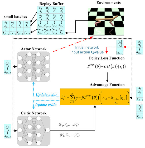
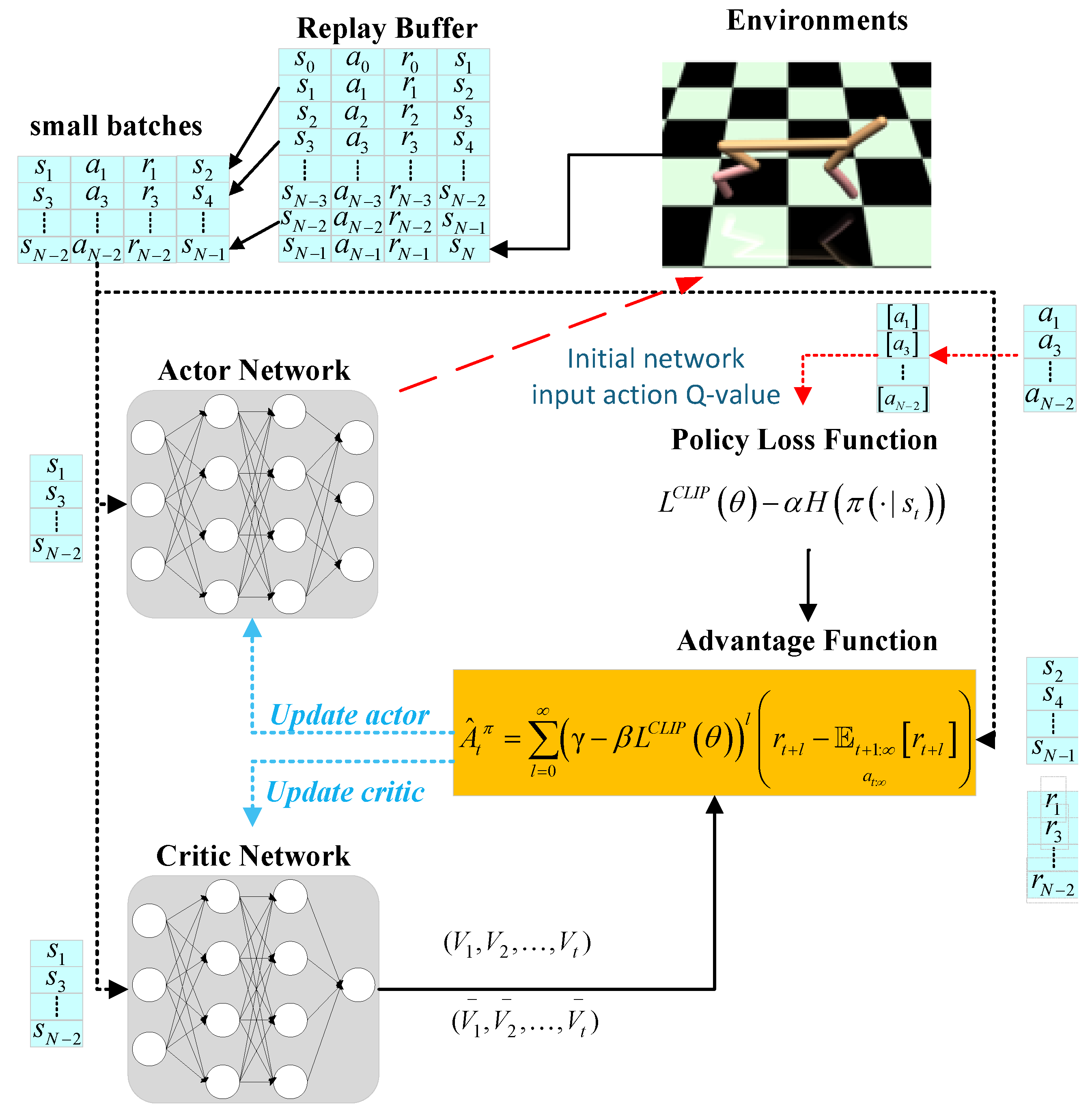
The proposed method dynamically adjusts the discount factor $\gamma$ for advantage estimation and incorporates policy entropy regularization, which reduces the need for manual hyperparameter tuning. This adaptive mechanism automatically tunes $\gamma$ throughout training to balance immediate and long-term rewards dynamically. In the initial training phases focused on exploration, immediate rewards expedite the development of effective strategies. Conversely, as the objective shifts towards maximizing long-term returns, a heightened emphasis on future rewards becomes paramount. Algorithm 1 summarizes the implementation procedure of A3E-PLE, and Figure 1 illustrates its overall framework.

Algorithm 1 A3E-PLE

Require:  Hyperparameters: K: number of iterations, $ϵ$: clipping factor, $\gamma$: discount factor   1: Initialize policy parameters $\theta$, value function parameters $\varphi$   2: for$k=0,1,2,\dots ,K-1$ do   3:       Execute policy ${\pi }_{{\theta }_k}$, collect trajectory set ${\mathcal{D}}_k=\left\{{\tau }_i\right\}$   4:       Compute discounted returns ${\widehat{G}}_t$ for all timesteps   5:       Calculate clipping loss ${\mathcal{L}}^{\mathrm{CLIP}}\left(\theta \right)$   6:       Compute advantage estimates $A_t$   7:       Compute target value function $V_t^{\mathrm{target}}$   8:       for each epoch do   9:           Compute policy entropy $\mathcal{H}\left({\pi }_{\theta }\right)$ 10:           Update policy parameters: ${\theta }_{k+1}\leftarrow \arg {\min }_{\theta }{\mathcal{L}}^{CLIP}\left(\theta \right)$ 11:           Update discount factor: $\gamma \leftarrow {\gamma }_{\mathrm{new}}$ 12:           Recompute advantages: $A_t\leftarrow A_{\mathrm{new}}$ 13:           Update value function: ${\varphi }_{k+1}\leftarrow \varphi -\eta {\nabla }_{\varphi }{\mathcal{L}}^{VF}$ 14:       end for 15: end for

Figure 1. Overview of the algorithmic framework.

As shown in Figure 1, the agent interacts with the environment using the current policy, generating trajectories consisting of states, actions, and rewards. These trajectories are fed into a feature extraction module that quantifies spatial complexity and motion constraints. The extracted features are used by a target entropy calculator to determine an entropy target suitable for the current environment, which in turn drives the update of the temperature coefficient $\alpha$. The updated entropy coefficient is simultaneously mapped to the GAE discount factor $\gamma$, dynamically adjusting the advantage estimation.

During the policy optimization phase, the algorithm employs an entropy-enhanced clipping mechanism and clipped importance sampling to balance the introduction of exploratory actions with the stability of policy updates. The final updated policy parameters are fed back into the environmental interaction loop, forming a continuous cycle of “perception–adjustment–optimization”. The closed-loop structure enables the algorithm to automatically adjust the discount factor in response to policy loss and entropy, thereby diminishing the necessity for manual tuning and intelligently resolving the exploration–exploitation trade-off in path planning.

This architecture enables adaptive advantage estimation, which substantially improves training stability and asymptotic performance in complex environments.

3.1. Policy Entropy Adjustment Policy Loss Function

Policy entropy serves as a metric to quantify the degree of uncertainty in action selection within a given state under a policy [37]. Essentially, when the probabilities of executing each potential action at the current state $s_t$ are more uniformly distributed, it indicates a heightened level of exploration by the policy, resulting in a correspondingly higher entropy value. The mathematical expression for computing policy entropy is given in Equation (13):

$$\begin{array}{c}\hfill H\left(\pi \left(·|s_t\right)\right)=E_{a\sim \pi \left(a_t|s_t\right)}\left[-\log \pi \left(a_t|s_t\right)\right]\end{array}$$

(13)

where $\left(\pi \left(a|s_t\right)\right)$ is the probability of executing action $a_t$ given state $s_t$, when modeling the policy using a Gaussian distribution with a standard deviation $\sigma$ [38], the formula for calculating policy entropy is presented in Equation (14):

$$\begin{array}{c}\hfill H\left(\pi \right)={\displaystyle \frac{1}{2}}\log \left(2\pi e{\sigma }^2\right)\end{array}$$

(14)

Entropy serves as a measure of the degree of uncertainty or unpredictability inherent in policy decisions. An increase in entropy indicates a shift towards more exploratory approaches in strategy formulation, while a decrease signifies the adoption of more definitive and less variable policies. The mathematical expression for calculating policy loss is presented in Equation (15):

$$\begin{array}{cc}\hfill L^{\mathrm{CLIP}}\left(\theta \right)& =-{\mathbb{E}}_t\left[\min \left(r_t\left(\theta \right)·A_t,\mathrm{clip}\left(r_t\left(\theta \right),1-ϵ,1+ϵ\right)·A_t\right)\right]\hfill \\ \hfill & -\alpha H\left(\pi \left(·|s_t\right)\right)\hfill \end{array}$$

(15)

where $\alpha$ is the policy entropy coefficient.

3.2. Reconstructing the Discount Factor $\gamma$ by Policy Loss

Traditional generalized advantage estimation relies on a fixed discount factor $\gamma$, which cannot dynamically adjust the credit assignment horizon according to the policy learning state. To address this limitation, this paper proposes a policy-loss-driven dynamic discount factor mechanism, which adjusts the weight of long-term returns in real time according to the fluctuation of policy loss, so as to balance the convergence speed and learning stability. In this section, we first review the basic formulation of GAE, then rigorously verify the theoretical validity of the dynamic discount factor mechanism, derive the mathematical expression of the adaptive advantage estimator, and finally introduce the boundary safeguard mechanism to ensure stable training.

The traditional advantage function estimation employs a fixed discount factor $\gamma$, which is defined as shown in Equation (16):

$$\begin{array}{c}\hfill {\widehat{A}}_t^{\pi ,\gamma }={\displaystyle \sum _{l=0}^{\infty }}{\gamma }^l{\delta }_{t+l}^V=-V^{\pi }\left(s_t\right)+{\displaystyle \sum _{l=0}^{\infty }}{\gamma }^l{r}_{t+l}\end{array}$$

(16)

The temporal difference error ${\delta }_{t+l}^V$ is defined as shown in Equation (17):

$$\begin{array}{c}\hfill {\delta }_{t+l}^V=r_{t+l}-\mathbb{E}\left[r_{t+l}\right]\end{array}$$

(17)

Substituting the TD error definition into Equation (16) yields Equation (18):

$$\begin{array}{c}\hfill {\widehat{A}}_t^{\pi ,\gamma }={\displaystyle \sum _{l=0}^{\infty }}{\gamma }^l\left(r_{t+l}-{\mathbb{E}}_{\begin{array}{c}{s}_{t+l+1}\\ a_{t+l}\end{array}}\left[r_{t+l}\right]\right)\end{array}$$

(18)

To dynamically adjust the balance between short-term and long-term rewards, this paper introduces a discount factor update mechanism driven by policy clipped loss:

$$\begin{array}{c}\hfill {\gamma }_{\mathrm{new}}={\gamma }_{\mathrm{old}}-\beta L^{\mathrm{CLIP}}\left(\theta \right)\end{array}$$

(19)

where $\beta$ is the update step coefficient, and $L^{\mathrm{CLIP}}\left(\theta \right)$ is the clipped surrogate loss function of PPO. In this work, we set the initial discount factor to $\gamma =0.99$ and the step coefficient to $\beta ={10}^{-5}$.

3.2.1. Theoretical Validity Analysis

To verify the theoretical soundness of the proposed dynamic discount factor mechanism, we analyze three aspects: optimization stability under bounded dynamic discount factors, gradient unbiasedness under non-stationary objectives, and the parameter range justification. In addition, an approximation error bound for the first-order binomial approximation is provided in the subsequent mathematical derivation.

(1) Optimization Stability Under Bounded Dynamic $\gamma$

The optimization framework of the proposed method is built upon the classical GAE and PPO formulations. Schulman et al. [19] defined the concept of a $\gamma$-just estimator and proved that for any discount factor $\gamma \in [0,1)$, the generalized advantage estimator maintains an unbiased estimate of the discounted policy gradient, which establishes the theoretical foundation of discounted policy gradient estimation. On this basis, Schulman et al. [15] further demonstrated that the clipped surrogate objective of PPO constructs a pessimistic lower bound of the original policy performance. By restricting the importance sampling ratio $r_t\left(\theta \right)$ within $[1-ϵ,1+ϵ]$, it mitigates catastrophic policy degradation and contributes to stable policy updates.

In the proposed algorithm, the dynamic discount factor $\gamma$ is strictly truncated to the interval $[0.85,0.99]$ throughout the training process. Since $\gamma$ is always constrained within $[0.85,0.99]\subset [0,1)$, the assumptions required by the original GAE framework remain satisfied.

Although $\gamma$ becomes time-varying, its update magnitude satisfies $|{\gamma }_k-{\gamma }_{k-1}|\le \beta C=\mathcal{O}\left(\beta \right)$, where C is a positive constant representing an upper bound of the clipped surrogate loss. Therefore, the proposed mechanism can be viewed as introducing a small perturbation to the original PPO/GAE framework, and does not significantly change its optimization dynamics.

Meanwhile, the update step size of $\gamma$ is set to an extremely small value $\beta ={10}^{-5}$, which makes the per-iteration variation of $\gamma$ on the order of ${10}^{-6}\sim {10}^{-5}$. This slow-varying characteristic ensures that the adjustment of $\gamma$ will not cause abrupt changes in the advantage estimation or the direction of the policy gradient. The core clipping mechanism of PPO remains effective, preventing excessively large policy updates and maintaining optimization stability.

(2) Gradient Unbiasedness Under Non-Stationary Objectives

The coupling of dynamic $\gamma$ and policy loss introduces mild non-stationarity into the optimization objective. In the following, we analyze its effect on policy gradient estimation and show that the induced perturbation remains bounded.

Let ${\widehat{A}}_t\left(\gamma \right)$ denote the advantage estimate under discount factor $\gamma$, and ${\gamma }_k$ denote the discount factor at the k-th iteration. The policy gradient at iteration k is:

$$g_k=\mathbb{E}\left[{\displaystyle \sum _{t=0}^{\infty }}{\widehat{A}}_t\left({\gamma }_k\right){\nabla }_{\theta }\log {\pi }_{\theta }\left(a_t\right|s_t)\right]$$

(20)

The gradient bias introduced by the change of $\gamma$ is:

$$\Delta g_k=g_k-g_k^{\mathrm{static}}=\mathbb{E}\left[{\displaystyle \sum _{t=0}^{\infty }}{\nabla }_{\theta }\log {\pi }_{\theta }\left(a_t\right|s_t)\left({\widehat{A}}_t\left({\gamma }_k\right)-{\widehat{A}}_t\left({\gamma }_{k-1}\right)\right)\right]$$

(21)

Since $|{\gamma }_k-{\gamma }_{k-1}|=\beta |L^{\mathrm{CLIP}}\left(\theta \right)|\le \beta C$, where C denotes the bounded maximum value of the clipped policy loss, it follows that $|{\gamma }_k-{\gamma }_{k-1}|=\mathcal{O}\left(\beta \right)$. Moreover, the advantage estimator ${\widehat{A}}_t\left(\gamma \right)={\sum }_{l=0}^{\infty }{\gamma }^l{\delta }_{t+l}^V$ is continuously differentiable with respect to $\gamma$ for $\gamma \in [0,1)$. A first-order Taylor expansion gives ${\widehat{A}}_t\left({\gamma }_k\right)-{\widehat{A}}_t\left({\gamma }_{k-1}\right)=\mathcal{O}({\gamma }_k-{\gamma }_{k-1})=\mathcal{O}\left(\beta \right)$. Substituting this result into Equation (21) gives $\Delta g_k=\mathcal{O}\left(\beta \right)$.

Therefore, the perturbation introduced by the adaptive discount factor is bounded by the update coefficient $\beta$. Since $\beta ={10}^{-5}$ is sufficiently small, the resulting gradient deviation is negligible compared with the intrinsic stochastic variance of policy gradient estimation. Consequently, the adaptive discount factor introduces only a mild perturbation to the optimization objective and does not significantly affect the approximate unbiasedness of the policy gradient in practice.

(3) Rationale for the $\gamma$ Boundary Setting

The setting of the dynamic discount-factor interval is based on empirical observations reported in previous reinforcement-learning studies.

François-Lavet et al. [28] investigated the influence of discount factors on the stability of deep reinforcement learning. Their results indicate that excessively large discount factors may amplify value-estimation errors and increase optimization variance, whereas excessively small discount factors tend to produce overly myopic policies that fail to capture long-term dependencies.

Their experiments further suggest that satisfactory performance is generally obtained when $\gamma$ lies approximately within the interval $[0.8,0.99]$.

Based on these observations, the proposed method constrains the dynamic discount factor to $\gamma \in [0.85,0.99]$, which provides a practical balance between long-term credit assignment and training stability while remaining within the feasible range required by the original GAE and PPO frameworks.

3.2.2. Mathematical Derivation of Adaptive Advantage Estimator

Based on the above theoretical guarantees and parameter settings, we substitute the dynamic discount factor into the GAE framework to derive the specific expression of the adaptive advantage estimator.

Substituting the dynamic discount factor into the advantage function yields:

$${\widehat{A}}_t^{\pi }={\displaystyle \sum _{l=0}^{\infty }}{\left(\gamma -\beta L^{\mathrm{CLIP}}\right)}^l{\delta }_{t+l}^V$$

(22)

We begin with a full binomial expansion of the dynamic discount term:

$${\left(\gamma -\beta L^{\mathrm{CLIP}}\right)}^l={\gamma }^l-l{\gamma }^{l-1}\beta L^{\mathrm{CLIP}}+{\displaystyle \sum _{i=2}^l}\left({\displaystyle \genfrac{}{}{0pt}{}{l}{i}}\right){\gamma }^{l-i}{\left(-\beta L^{\mathrm{CLIP}}\right)}^i$$

(23)

We further quantify the truncation error of the first-order approximation used in Equation (22) by analyzing the magnitude of the higher-order remainder. Define the remainder term as

$$R_l={\displaystyle \sum _{i=2}^l}\left({\displaystyle \genfrac{}{}{0pt}{}{l}{i}}\right){\gamma }^{l-i}{\left(-\beta L^{\mathrm{CLIP}}\right)}^i$$

(24)

Taking absolute values and applying the triangle inequality yields:

$$\left|R_l\right|\le {\displaystyle \sum _{i=2}^l}\left({\displaystyle \genfrac{}{}{0pt}{}{l}{i}}\right){\gamma }^{l-i}{\left(\beta \left|L^{\mathrm{CLIP}}\right|\right)}^i$$

(25)

Since $0<\gamma <1$ and the clipped surrogate loss is bounded by the clipping mechanism, satisfying $\left|L^{\mathrm{CLIP}}\right|\le C$, we substitute the upper bound into the summation to obtain

$$\left|R_l\right|\le {\displaystyle \sum _{i=2}^l}\left({\displaystyle \genfrac{}{}{0pt}{}{l}{i}}\right){\gamma }^{l-i}{\left(\beta C\right)}^i.$$

(26)

Since $\beta C\ll 1$, the magnitude of each term in the summation decays rapidly as the order i increases. The term with the lowest power $i=2$ is the dominant term that determines the overall magnitude of the remainder. Substituting the binomial coefficient $\left({\displaystyle \genfrac{}{}{0pt}{}{l}{2}}\right)={\displaystyle \frac{l(l-1)}{2}}$, the leading second-order term of the remainder takes the form of ${\displaystyle \frac{l(l-1)}{2}}{\gamma }^{l-2}{\left(\beta C\right)}^2$.

All terms with $i\ge 3$ are higher-order small quantities compared with the second-order term. Therefore, the magnitude of the remainder is bounded by

$$R_l=\mathcal{O}\left({\left(\beta C\right)}^2\right)$$

(27)

The above analysis shows that the truncation error is of second order with respect to the perturbation magnitude. Given that $\beta ={10}^{-5}$, the contribution of the second-order and higher-order terms is negligible compared with the first-order term. Thus, the higher-order remainder is neglected in the subsequent derivation, and we adopt the first-order approximation:

$${\left(\gamma -\beta L^{\mathrm{CLIP}}\right)}^l\approx {\gamma }^l-l{\gamma }^{l-1}\beta L^{\mathrm{CLIP}}$$

(28)

Substituting the first-order approximation back into Equation (22), we obtain the decomposed form of the adaptive advantage estimator:

$${\widehat{A}}_t^{\pi }\approx \underset{\mathrm{Original}\mathrm{GAE}\mathrm{term}}{\underbrace{\sum _{l=0}^{\infty }{\gamma }^l{\delta }_{t+l}^V}}-\beta L^{\mathrm{CLIP}}\underset{\mathrm{Time}\text{-}\mathrm{sensitive}\mathrm{correction}\mathrm{term}}{\underbrace{\sum _{l=1}^{\infty }l{\gamma }^{l-1}{\delta }_{t+l}^V}}$$

(29)

It can be seen that the adaptive advantage estimator consists of the original GAE component and an additional loss-dependent correction term. As the policy loss increases, the influence of the correction term becomes more pronounced, enabling adaptive adjustment of the effective discounting behavior. Conversely, when the policy loss becomes small, the adaptive estimator gradually approaches the standard GAE formulation.

3.2.3. Boundary Safeguard Mechanism

Although the dynamic $\gamma$ has a small update step size, to avoid boundary risks during long-term iterative training, we design a hard truncation mechanism to ensure that $\gamma$ always stays within the predefined admissible interval. The specific rules are as follows:

(1) When the updated ${\gamma }_{\mathrm{new}}>0.99$, set ${\gamma }_{\mathrm{new}}=0.99$ to prevent value function overestimation and training instability.

(2) When the updated ${\gamma }_{\mathrm{new}}<0.85$, set ${\gamma }_{\mathrm{new}}=0.85$ to avoid the policy becoming excessively short-sighted and failing to learn long-term sequential behaviors.

This dual safeguard of slow-varying updates and boundary truncation ensures that the dynamic discount factor always remains within the feasible range $[0.85,0.99]$. Since the variation of $\gamma$ between consecutive updates is bounded by $\mathcal{O}\left(\beta \right)$, the proposed mechanism introduces only a mild perturbation to the original PPO optimization process. Therefore, the optimization stability of PPO is expected to be preserved in practice.

3.2.4. Implementation Workflow of the Dynamic Adjustment Mechanism

To further clarify the operational logic of the proposed dynamic adjustment mechanism and improve methodological transparency, this subsection details its implementation workflow and execution timing within the training pipeline, corresponding to the pseudocode presented in Algorithm 1.

The dynamic discount factor is updated during each training epoch according to a fixed execution sequence that is tightly coupled with the policy and value network optimization process:

(1) After collecting a full batch of trajectories, compute the initial advantage estimates and the clipped surrogate loss based on the current policy and the discount factor inherited from the previous iteration.

(2) In each inner training epoch, first calculate the batch-averaged policy entropy and update the policy network parameters using the policy loss defined in Equation (15).

(3) Compute the average clipped surrogate loss across all samples in the current batch, and update the discount factor according to Equation (19): ${\gamma }_{\mathrm{new}}={\gamma }_{\mathrm{old}}-\beta L^{\mathrm{CLIP}}\left(\theta \right)$, where $\beta ={10}^{-5}$ is a small fixed update step coefficient. The clipped surrogate loss is employed as the feedback signal because it directly reflects the current optimization status of the policy and provides a stable indicator for adaptive discount factor adjustment during training.

(4) Apply the boundary truncation safeguard described in Section 3.2.3 to constrain ${\gamma }_{\mathrm{new}}$ within the interval $[0.85,0.99]$, ensuring numerical stability and preventing invalid discount factor values.

(5) Recalculate the generalized advantage estimates for the current batch of trajectories using the updated discount factor.

(6) Update the value network parameters using the recomputed advantage estimates and the corresponding target returns.

Consistent with Algorithm 1, the updated discount factor is immediately incorporated into the advantage estimation process before value function optimization. This design enables the value network to utilize the most recent reward horizon information while preserving the stability of policy optimization.

Notably, the discount factor is updated once per inner epoch rather than per mini-batch, which avoids excessive fluctuations in advantage estimation caused by overly frequent updates and preserves the stability of value function optimization. The update step coefficient $\beta$ is set to an extremely small value, such that the variation of $\gamma$ per iteration stays on the order of ${10}^{-6}$ to ${10}^{-5}$, ensuring a slow and smooth adaptive adjustment process.

In addition, the entropy regularization term uses a fixed coefficient $\alpha =0.01$ throughout training and is incorporated into every policy update step. The entropy regularization mechanism operates independently of the dynamic discount factor adjustment mechanism. Specifically, the entropy term promotes exploration by controlling policy randomness, whereas the adaptive discount factor improves the accuracy of return and advantage estimation through dynamic reward horizon adjustment. Together, these two mechanisms contribute to enhanced learning efficiency and training stability.

4. Simulation

4.1. Environments

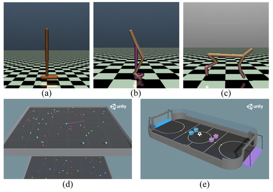
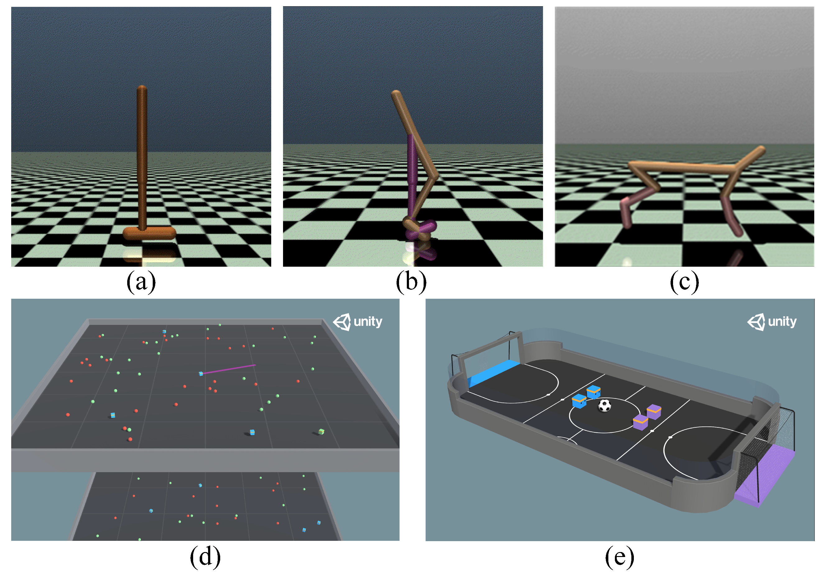
Ablation experiments were conducted on OpenAI Gym’s MuJoCo and Unity ML-Agents environments to validate the effectiveness of A3E-PLE, with average cumulative reward as the primary evaluation metric. Four algorithm variants were compared: (1) GAE (baseline): standard PPO with fixed GAE; (2) GAE-entropy: PPO with GAE and entropy regularization for enhanced exploration; (3) A3E-PL: PPO with adaptive policy-loss-based advantage estimation; (4) A3E-PLE: the full proposed method integrating both mechanisms. The five experimental environments are illustrated in Figure 2, comprising three MuJoCo continuous control tasks (Hopper-v2, Walker2d-v2, HalfCheetah-v2) and two ML-Agents multi-agent tasks (Food Collector, Soccer Twos).All experiments were implemented in Python 3.7. The MuJoCo continuous control environments (Hopper-v2, Walker2d-v2, HalfCheetah-v2) were built on the OpenAI Gym v0.19.0 framework with the mujoco-py v1.50.1.0 interface. The two multi-agent environments were developed using Unity Engine (2022.3.52f1c1) and the ML-Agents Toolkit (release_11). All code was developed and debugged in PyCharm Community Edition 2023.3.5. The maximum training steps were set to 3 million for MuJoCo environments, 2 million for Food Collector, and 12 million for Soccer Twos. The detailed hyperparameter settings are listed in Table 2.

Figure 2. Three simulated physical environments for OpenAI Gym MuJoCo [39] and two complex decision- making environments for robot control and ML-Agents [40]. (a) Hopper. (b) Walker2d. (c) HalfCheetah. (d) Food Collector. (e) Soccer Twos. The MuJoCo environments were built with OpenAI Gym (v0.19.0; https://gymnasium.farama.org/) and MuJoCo (v1.50.1.0; https://mujoco.org/), while the ML-Agents environments were developed using the ML-Agents Toolkit (release_11; https://github.com/Unity-Technologies/ml-agents) on the Unity engine (2022.3.52f1c1; https://unity.com/) [41]. All development was conducted in a Python 3.7 environment using PyCharm Community Edition (2023.3.5; https://www.jetbrains.com/pycharm/) [42].

Table 2. Hyperparameter settings.

Name	Value
learning rate	3 × 10−4
batch size	2048
$\lambda$	0.95
entropy coef	0.01

To simulate physical environments and robot control tasks, three tasks from the OpenAI Gym MuJoCo environment were utilized: Hopper-v2, Walker2d-v2, and HalfCheetah-v2.

Figure 2a illustrates the Hopper, a two-dimensional, single-legged model designed to train an agent for executing forward jumps. The reward system comprises three components: a constant reward, a reward for forward movement, and a penalty for excessive actions. The agent’s actions involve applying torque to the thigh, supporting leg, and foot rotors. The observations, which prioritize positional values over velocities, encompass the positions and velocities of various body parts. By default, the observation data is structured as an array with 11 elements.

Figure 2b presents the Walker2d, an advancement of the Hopper that features additional supporting legs, enabling bipedal forward walking. This two-dimensional bipedal model incorporates a three-part reward structure: a base reward, a reward for forward progression, and a penalty for excessive actions. The agent’s actions involve applying torque to six hinges, facilitating coordinated movement of the two sets of feet, legs, and thighs in the forward direction. The observations capture the positional values of various walker body parts, followed by their respective velocities, with positions given precedence over velocities. The default observation format is an array comprising 17 elements.

Figure 2c illustrates the HalfCheetah, a two-dimensional quadrupedal robot structured with 9 links and 8 joints. The primary goal is to optimize forward running speed by applying torque to the joints, with rewards positively correlated to forward motion and negatively to backward motion. The cheetah’s torso and head remain stationary, allowing torque manipulation solely on the remaining 6 joints: the front and rear thighs, shins, and feet. The objective is to train the cheetah robot to achieve maximum forward velocity. The reward mechanism encompasses forward-oriented incentives and penalties for excessive actions. The actions consist of applying torque between the various links. The observation space encompasses the positional states and velocities of various cheetah body parts, with positional values preceding velocity values in the array. As a default, the observation format is an array of 17 elements.

The two multi-agent environments are built on the Unity ML-Agents Toolkit release _11, which provides standardized 3D simulation scenarios with rich agent interactions and physics-based dynamics.

Figure 2d illustrates the Food Collector, a multi-agent setting where agents compete to collect green food spheres while avoiding red ones. Agents must develop strategies to maximize green sphere collection and can emit laser beams to disrupt competitors. Collecting a green sphere yields $+1$ reward, whereas encountering a red sphere incurs $-1$ penalty. The action space encompasses three continuous controls for navigation (forward/backward, lateral, and rotation) along with a discrete command to activate the laser. The observation space utilizes a grid sensor configuration consisting of 40 × 40 grids along the z- and x-axes, respectively, with a single grid along the y-axis. The sensor detects food, harmful food, rival agents, frozen agents, walls, and null observations, summing to 960 total observation dimensions (40 × 40 × 6). Training is conducted over a maximum of 2,000,000 time steps, with each episode capped at 10,000 steps, across 200 episodes.

Figure 2e showcases Soccer Twos, a 2 vs. 2 soccer simulation in which agents strive to score in the opponent’s goal while defending their own. Each successful score awards $+1$ reward and reset at the beginning of each round, while goals conceded incur $-1$ penalty. Agents have 27 discrete actions for movement and rotation. Their observations comprise 336 values, capturing 11 forward and 3 backward ray projections, each detecting 6 object types and distances. The forward projections span 264 dimensions across stacks, while backward projections contribute 72. Training spans 12 million steps, with episodes limited to 10,000 steps over 1200 rounds.

4.2. Network Architectures

The policy and value networks utilize distinct architectures specifically optimized for the observation characteristics of their respective environments. As detailed in Table 3, the MuJoCo agent uses a fully connected network (FCN) with an input layer matching the state dimension, two hidden layers of 256 units each, and separate output layers for policy (action dimension) and value (1 unit), totaling 4 layers. In contrast, the ML-Agent uses a convolutional network (CNN) that begins with a convolutional layer (32 channels, 5 × 5 kernel) processing visual inputs, followed by another convolutional layer (64 channels, 3 × 3 kernel), and two fully connected hidden layers of 512 units. Its policy output is a fully connected layer (action dimension), while the value output uses a multi-head fully connected architecture, resulting in a deeper 6-layer network.

Table 3. Network Architecture Specifications.

Network Type	MuJoCo (FCN)	ML-Agent (CNN)
Input Layer	FC (state_dim)	Conv (32ch@5×5) + FC (vector)
Hidden Layers	FC × 2 (256 units)	Conv (64ch@3×3) + FC × 2 (512 units)
Output Layer	Policy: FC (action_dim)	Policy: FC (action_dim)
	Value: FC (1)	Value: Multi-head Fully Connected FC
Total Layers	4	6

All experiments used a fixed random seed of 10 to ensure consistent initialization across all compared methods. This controlled setup mitigates confounding effects from random initialization and enables fair pairwise performance comparisons.

4.3. Simulation Results and Analysis

Table 4 lists explanations of various algorithm abbreviations.

Table 4. Algorithm Component Comparison.

Algorithm	Adaptive $\mathit{\gamma }$	Entropy Exploration	Base
GAE (Baseline)	✕	✕	PPO
GAE-entropy	✕	✓	PPO
A3E-PL	✓	✕	PPO
A3E-PLE (Full Proposed)	✓	✓	PPO

Note: ✓ indicates the inclusion of the corresponding component, and ✕ means the component is not adopted.

The four variants differ in two dimensions: adaptive discount factor and entropy regularization, as detailed in Table 4. GAE serves as the baseline with fixed parameters and no entropy term. GAE-entropy adds only entropy regularization. A3E-PL includes only the adaptive advantage estimation mechanism. A3E-PLE integrates both innovations as the full proposed method.

All learning curves are processed via exponential smoothing to balance trend responsiveness and noise suppression. The formulation is given in Equation (30):

$$\begin{array}{c}\hfill S_t=\mu ·x_t+\left(1-\mu \right)·S_{t-1}\end{array}$$

(30)

where $S_t$ is the smoothed value at time t, $x_t$ is the actual observation, $S_{t-1}$ is the smoothed value at the previous time step, and $\mu \in [0,1]$ is the smoothing factor.

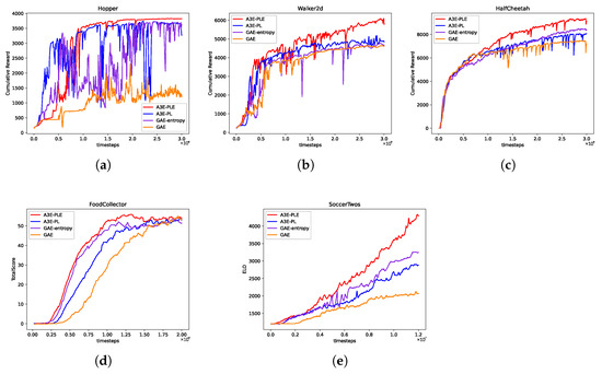
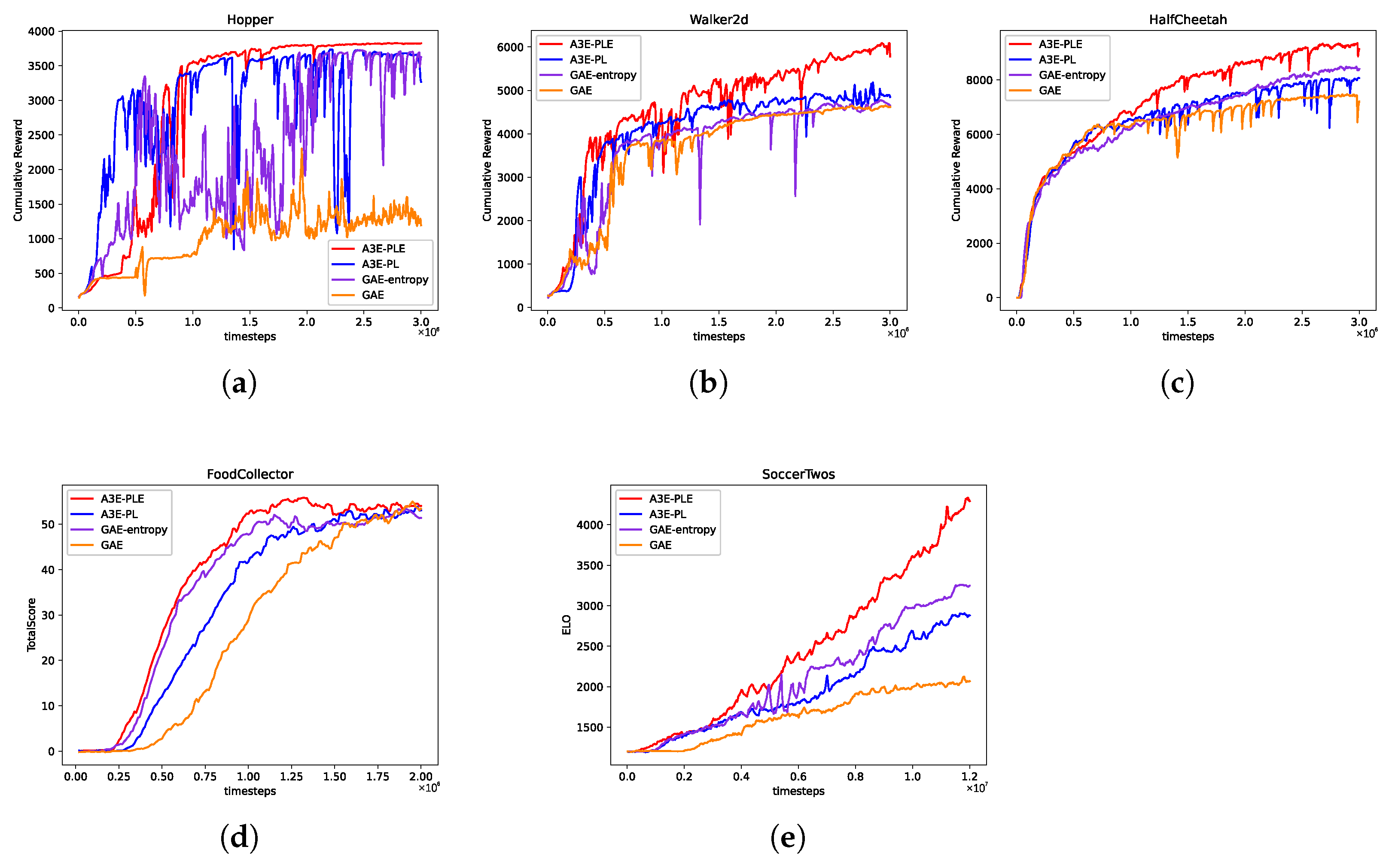
Table 5 and Figure 3 present the experimental results of all algorithm variants across the five environments. Notably, the discount factor $\gamma$ was fixed at 0.99 for both GAE and GAE-entropy. As shown in Figure 3b,c, A3E-PLE achieves the highest cumulative rewards, reaching approximately 6188 in Walker2d and 9418 in HalfCheetah, demonstrating substantial improvement over the other three variants.

Table 5. Comparison of the maximum cumulative rewards in different environments for the four variants.

Environment	Maximum Average Reward
	A3E-PLE	A3E-PL	GAE-entropy	GAE
Hopper	3834	3751	3728	2693
Walker2d	6188	5623	4791	4672
HalfCheetah	9418	8206	8595	7564
Food Collector	67	67	64	63.0
Soccer Twos	4335	2908	3258	2126

Note: Bold values denote the optimal reward performance within each corresponding environment.

Figure 3. Learning curves of different algorithms across five environments. (a) Hopper. (b) Walker2d. (c) HalfCheetah. (d) Food Collector. (e) Soccer Twos.

In Figure 3, the solid lines represent the exponentially smoothed reward values, while the shaded areas indicate the standard deviation within a sliding window (window size = 100 steps). This visualization captures both volatility and stability of the learning process throughout training. Although we used a fixed random seed due to computational constraints, the sliding window standard deviation provides valuable insights into the algorithm’s consistency and learning dynamics. The narrower shaded regions observed for A3E-PLE across environments suggest more stable and consistent learning progress compared to other variants, particularly during the later stages of training where it achieves and maintains higher performance plateaus.

In the Hopper environment depicted in Figure 3a, A3E-PLE does not outperform GAE-entropy and A3E-PL in cumulative reward during the first 700,000 steps. However, GAE-entropy and A3E-PL exhibit large performance fluctuations in this phase, indicating unstable training processes. In contrast, A3E-PLE demonstrated a remarkable degree of training stability and efficiency, consistently maintaining cumulative rewards above 3800. Despite starting behind, A3E-PLE’s stability allowed it to gradually outpace GAE-entropy and A3E-PL, which hovered around 3700. This trend underscores not only the inherent stability advantages of A3E-PLE but also its ability to sustain and ultimately surpass the performance of the other two approaches, demonstrating its robustness and effectiveness over extended training sessions.

In Figure 3d, while the final cumulative rewards indicate only marginal differences among the methods, A3E-PLE stands out for its remarkable capacity to rapidly stabilize at relatively high performance levels. However, this subtle advantage in the final outcome can be attributed to the inherent limitations posed by the discrete nature of the action space. This discreteness may constrain the precision and flexibility of the robot’s decision-making, especially in response to laser hits, ultimately limiting the extent of A3E-PLE’s performance gains over the other methods. Despite these constraints, A3E-PLE’s ability to swiftly stabilize showcases its resilience within the given action space framework.

In Figure 3e, the Soccer Twos environment employs the ELO rating system as a comparative metric. The ELO rating system [43] has become a widely accepted standard for assessing the proficiency of competitors across various activities. It effectively reflects the strengths of players and fosters equilibrium in intricate decision-making scenarios, thereby offering more discernible comparative outcomes. The results show that the final ELO rating of A3E-PLE is approximately twice that of the GAE baseline, verifying its significant advantage in competitive tasks.

In analyzing Table 6, which compares the sample efficiency of the four variants in terms of steps required to reach predefined target scores. Among the ten target scores across all environments, A3E-PLE ranks first (requires the fewest steps) in six cases. Although it did not consistently secure the top spot in mid-stage objective scores within certain environments, A3E-PLE distinguished itself by requiring significantly fewer time steps to reach the final objectives. This underscores its inherent adaptability and enables swift adjustments in policy optimization, which translates into enhanced performance efficiency.

Table 6. Comparison of time steps required for convergence across algorithm variants.

Environment	Target Score	Time Steps to Reach Target Score
		A3E-PLE	A3E-PL	GAE-Entropy	GAE
Hopper	2000	645,000	205,000	430,000	1,445,000
	3500	880,000	1,095,000	1,310,000	-
Walker2d	3000	280,000	275,000	300,000	545,000
	5000	1,230,000	2,605,000	-	-
HalfCheetah	6000	710,000	615,000	890,000	590,000
	8000	1,425,000	2,525,000	2,280,000	-
Food Collector	30	430,000	640,000	460,000	810,000
	60	910,000	930,000	1,030,000	1,310,000
Soccer Twos	1500	2,760,000	2,960,000	2,740,000	4,110,000
	3000	8,440,000	-	10,090,000	-

Note: Bold values represent the minimum convergence time steps under the corresponding target score, indicating the fastest convergence speed among all algorithms.

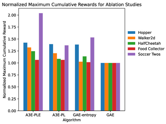
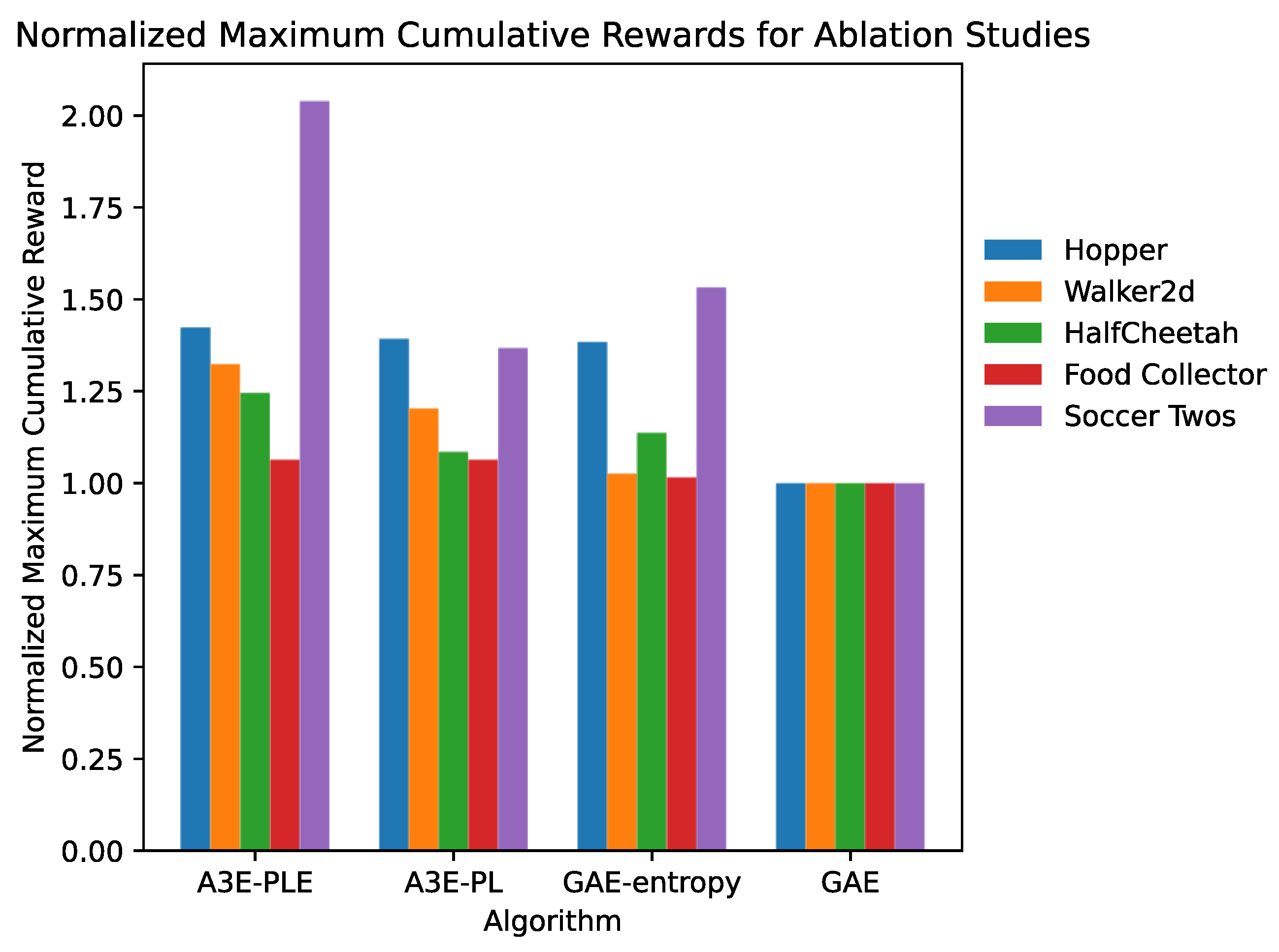
Figure 4 presents the ablation study results in terms of normalized maximum cumulative rewards. Since raw reward scales vary significantly across different environments, all results are normalized to the GAE baseline (set to 1.0): the maximum reward of each algorithm in an environment is divided by that of GAE in the same environment.

Figure 4. Normalized maximum cumulative rewards of the four ablation algorithms across five environments.

Quantitatively, A3E-PLE consistently outperforms the GAE baseline across all environments, with relative improvements of 42.34% on Hopper, 32.44% on Walker2d, 24.51% on HalfCheetah, 6.35% on Food Collector, and 103.93% on Soccer Twos. These results validate the effectiveness and generalization ability of the proposed method.

Overall, A3E-PLE consistently demonstrates competitive or even superior performance in reaching predefined target scores across various environments and task complexities. Its adaptability to different objectives and environments highlights its potential as an effective reinforcement learning algorithm.

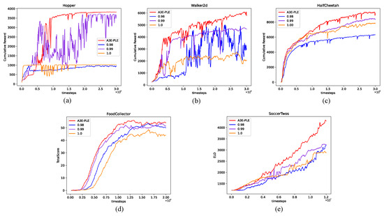
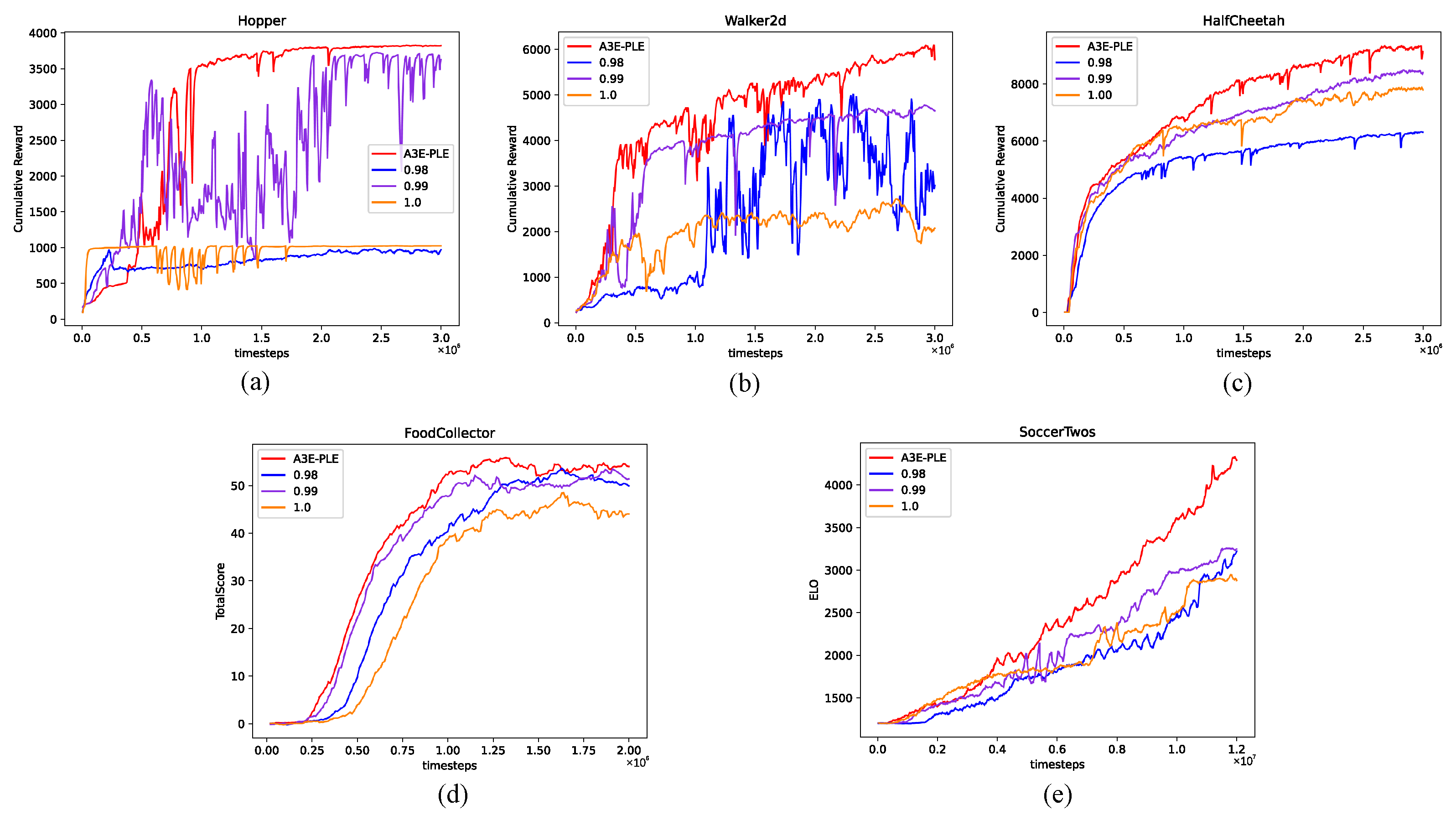
As demonstrated in Table 7 and Figure 5, the performance of A3E-PLE was compared against that achieved using fixed discount factors of $\gamma =[0.98,0.99,1.00]$. Each experimental setup incorporated policy entropy, with the primary variable of interest being the influence of the discount factor on the results. Previous research by Schulman et al. [19] has suggested that optimal performance often lies within the range of $\gamma$ values from 0.98 to 1, with 0.99 frequently used as a standard. Consequently, our experiments focused on these three fixed $\gamma$ values.

Table 7. Comparison of maximum cumulative rewards for four discount factors $\gamma$ different environments.

Environment	Maximum Average Reward
	A3E-PLE	0.98	0.99	1.00
Hopper	3834	1009	3728	1027
Walker2d	6188	5510	4791	2756
HalfCheetah	9418	6366	8595	7940
Food Collector	67	67	64	63
Soccer Twos	4335	3227	3258	2946

Note: Bold values represent the optimal maximum average reward obtained within each corresponding environment.

Figure 5. Compares the cumulative rewards for discount factors $\gamma$ as A3E-PLE, 0.98, 0.99, and 1.00. (a) Hopper. (b) Walker2d. (c) HalfCheetah. (d) Food Collector. (e) Soccer Twos.

The results presented in Table 7 reveal a notable enhancement in the maximum average reward achieved by A3E-PLE compared to the fixed discount factors. Specifically, A3E-PLE outperforms the $\gamma =0.99$ baseline by significant margins: 2.84% in Hopper, 29.16% in Walker2d, 9.58% in HalfCheetah, 4.69% in Food Collector, and a substantial 33.06% in Soccer Twos.

Furthermore, as the target scores increase in difficulty, the advantages of A3E-PLE become even more pronounced. It achieves the target scores more efficiently, underscoring the effectiveness of its adaptive adjustment of the estimator parameter $\gamma$. This finding validates that the dynamic adaptation of $\gamma$ within A3E-PLE effectively addresses the challenges posed by varying task complexities and accelerates the learning process.

5. Conclusions

This paper proposes A3E-PLE, an adaptive advantage estimation algorithm for reinforcement-learning-based robot motion control. To address the limitations of fixed discount factors and insufficient exploration in standard PPO with GAE, the proposed method integrates two core components: a policy-loss-driven dynamic discount factor mechanism and entropy regularization for Gaussian-distributed policies.

Theoretical analysis indicates that the adaptive modulation of $\gamma$ adjusts the effective credit assignment horizon according to the evolving policy optimization status, while the entropy regularization term promotes sufficient exploration and maintains stable policy updates.

Extensive experiments were conducted on five benchmark environments, including three MuJoCo continuous locomotion tasks (Hopper-v2, Walker2d-v2, HalfCheetah-v2) and two Unity ML-Agents multi-agent scenarios (Food Collector and Soccer Twos). The results demonstrate that A3E-PLE consistently outperforms the fixed-$\gamma$ GAE baseline in terms of both asymptotic performance and sample efficiency. In particular, the method exhibits improved learning stability and stronger performance gains in complex multi-agent settings, which verifies its strong generalization across both single-agent continuous control and multi-agent competitive tasks.

From an implementation perspective, A3E-PLE is highly compatible with standard PPO implementations and introduces negligible computational overhead, facilitating practical deployment in robotic systems.

For future work, two promising directions are outlined. First, the linear update rule for $\gamma$ can be further improved by exploring more theoretically grounded adaptive weighting strategies based on policy optimization signals. Second, the method will be extended to physical robotic platforms, including legged robots and industrial manipulators, to evaluate its robustness under real-world sensor noise and environmental uncertainties.

Overall, the proposed A3E-PLE provides a simple yet effective mechanism for adaptive advantage estimation, providing a lightweight, easy-to-deploy solution for improving PPO-based reinforcement learning in robotic motion control applications.

References

- Yu, Y.; Li, J.; Solomon, S.A.; Min, J.; Tu, J.; Guo, W.; Xu, C.; Song, Y.; Gao, W. All-printed soft human-machine interface for robotic physicochemical sensing. Sci. Robot. 2022, 7, eabn0495. [Google Scholar] [PubMed]
- Li, Y.; He, J.; Chen, C.; Guan, X. Intelligent physical attack against mobile robots with obstacle-avoidance. IEEE Trans. Robot. 2022, 39, 253–272. [Google Scholar] [CrossRef] [Scilit]
- Bijjahalli, S.; Sabatini, R.; Gardi, A. Advances in intelligent and autonomous navigation systems for small UAS. Prog. Aerosp. Sci. 2020, 115, 100617. [Google Scholar] [CrossRef] [Scilit]
- Zhao, Y.; Lian, J.; Wang, D. Adaptive risk-averse reinforcement learning for cooperative navigation of multiple robots. Inf. Sci. 2026, 736, 123105. [Google Scholar] [CrossRef] [Scilit]
- Wang, J.; Pradhan, M.R.; Gunasekaran, N. Machine learning-based human-robot interaction in ITS. Inf. Process. Manag. 2022, 59, 102750. [Google Scholar] [CrossRef] [Scilit]
- Lopez-Sanchez, I.; Moreno-Valenzuela, J. PID control of quadrotor UAVs: A survey. Annu. Rev. Control 2023, 56, 100900. [Google Scholar] [CrossRef] [Scilit]
- Feng, H.; Jiang, J.; Chang, X.; Yin, C.; Cao, D.; Yu, H.; Li, C.; Xie, J. Adaptive sliding mode controller based on fuzzy rules for a typical excavator electro-hydraulic position control system. Eng. Appl. Artif. Intell. 2023, 126, 107008. [Google Scholar] [CrossRef] [Scilit]
- Zamani, A.A.; Etedali, S. Seismic structural control using magneto-rheological dampers: A decentralized interval type-2 fractional-order fuzzy PID controller optimized based on energy concepts. ISA Trans. 2023, 137, 288–302. [Google Scholar] [PubMed]
- Yao, Z.; Yu, J.; Zhang, J.; He, W. Graph and dynamics interpretation in robotic reinforcement learning task. Inf. Sci. 2022, 611, 317–334. [Google Scholar] [CrossRef] [Scilit]
- Siegel, N.Y.; Springenberg, J.T.; Berkenkamp, F.; Abdolmaleki, A.; Neunert, M.; Lampe, T.; Hafner, R.; Heess, N.; Riedmiller, M. Keep doing what worked: Behavioral modelling priors for offline reinforcement learning. arXiv 2020, arXiv:2002.08396. [Google Scholar]
- Watkins, C.J.; Dayan, P. Q-learning. Mach. Learn. 1992, 8, 279–292. [Google Scholar] [CrossRef] [Scilit]
- Mnih, V.; Kavukcuoglu, K.; Silver, D.; Rusu, A.A.; Veness, J.; Bellemare, M.G.; Graves, A.; Riedmiller, M.; Fidjeland, A.K.; Ostrovski, G.; et al. Human-level control through deep reinforcement learning. Nature 2015, 518, 529–533. [Google Scholar] [CrossRef] [Scilit] [PubMed]
- Moghaddam, A.R.; Kebriaei, H. Expected Policy Gradient for Network Aggregative Markov Games in Continuous Space. IEEE Trans. Neural Netw. Learn. Syst. 2024, 36, 7372–7381. [Google Scholar] [CrossRef] [Scilit]
- Schulman, J.; Levine, S.; Abbeel, P.; Jordan, M.; Moritz, P. Trust region policy optimization. In Proceedings of the International Conference on Machine Learning, PMLR, Lille, France, 6–11 July 2015; pp. 1889–1897. [Google Scholar]
- Schulman, J.; Wolski, F.; Dhariwal, P.; Radford, A.; Klimov, O. Proximal policy optimization algorithms. arXiv 2017, arXiv:1707.06347. [Google Scholar]
- Jiang, Y.; Li, C.; Dai, W.; Zou, J.; Xiong, H. Variance reduced domain randomization for reinforcement learning with policy gradient. IEEE Trans. Pattern Anal. Mach. Intell. 2023, 46, 1031–1048. [Google Scholar] [CrossRef] [Scilit]
- Mnih, V.; Badia, A.P.; Mirza, M.; Graves, A.; Lillicrap, T.; Harley, T.; Silver, D.; Kavukcuoglu, K. Asynchronous methods for deep reinforcement learning. In Proceedings of the International Conference on Machine Learning, PMLR, New York, NY, USA, 19–24 June 2016; pp. 1928–1937. [Google Scholar]
- Babaeizadeh, M.; Frosio, I.; Tyree, S.; Clemons, J.; Kautz, J. Reinforcement learning through asynchronous advantage actor-critic on a gpu. arXiv 2016, arXiv:1611.06256. [Google Scholar]
- Schulman, J.; Moritz, P.; Levine, S.; Jordan, M.; Abbeel, P. High-dimensional continuous control using generalized advantage estimation. arXiv 2015, arXiv:1506.02438. [Google Scholar]
- Pan, H.R.; Gürtler, N.; Neitz, A.; Schölkopf, B. Direct advantage estimation. Adv. Neural Inf. Process. Syst. 2022, 35, 11869–11880. [Google Scholar] [CrossRef] [Scilit]
- Park, J.; Han, S. Reinforcement learning with multimodal advantage function for accurate advantage estimation in robot learning. Eng. Appl. Artif. Intell. 2023, 126, 107019. [Google Scholar] [CrossRef] [Scilit]
- Zhang, J.; Han, S.; Xiong, X.; Zhu, S.; Lü, S. Explorer-Actor-Critic: Better actors for deep reinforcement learning. Inf. Sci. 2024, 662, 120255. [Google Scholar]
- Zhang, P.; Zhao, L.; Liu, G.; Bian, J.; Huang, M.; Qin, T.; Liu, T.Y. Independence-Aware Advantage Estimation. In Proceedings of the 30th International Joint Conference on Artificial Intelligence, Montreal, QC, Canada, 21–26 August 2021; Paper presented at IJCAI-21. pp. 3349–3355. [Google Scholar]
- Chen, Y.; Zhang, F.; Liu, Z. Adaptive bias-variance trade-off in advantage estimator for actor–critic algorithms. Neural Netw. 2024, 169, 764–777. [Google Scholar] [PubMed]
- Naik, A.; Shariff, R.; Yasui, N.; Yao, H.; Sutton, R.S. Discounted reinforcement learning is not an optimization problem. arXiv 2019, arXiv:1910.02140. [Google Scholar]
- Alexander, W.H.; Brown, J.W. Hyperbolically discounted temporal difference learning. Neural Comput. 2010, 22, 1511–1527. [Google Scholar] [CrossRef] [Scilit] [PubMed]
- Zinzuvadiya, M. Adaptive Discounting in Reinforcement Learning. Master’s Thesis, University of New Haven, West Haven, CT, USA, 2020. [Google Scholar]
- François-Lavet, V.; Fonteneau, R.; Ernst, D. How to discount deep reinforcement learning: Towards new dynamic strategies. arXiv 2015, arXiv:1512.02011. [Google Scholar]
- Thomas, P. Bias in natural actor-critic algorithms. In Proceedings of the International Conference on Machine Learning, PMLR, Beijing, China, 21–26 June 2014; pp. 441–448. [Google Scholar]
- Liu, J. On the convergence of reinforcement learning with Monte Carlo Exploring Starts. Automatica 2021, 129, 109693. [Google Scholar] [CrossRef] [Scilit]
- Yang, G.; Chen, X.; Yang, S.; Wang, H.; Dong, S.; Gao, Y. Online attentive kernel-based temporal difference learning. arXiv 2022, arXiv:2201.09065. [Google Scholar]
- Dayan, P. The convergence of TD (λ) for general λ. Mach. Learn. 1992, 8, 341–362. [Google Scholar] [CrossRef] [Scilit]
- Wu, Z.; Yu, C.; Chen, C.; Hao, J.; Zhuo, H.H. Plan to predict: Learning an uncertainty-foreseeing model for model-based reinforcement learning. Adv. Neural Inf. Process. Syst. 2022, 35, 15849–15861. [Google Scholar]
- Hao, D.; Zhang, D.; Shi, Q.; Li, K. Entropy regularized actor-critic based multi-agent deep reinforcement learning for stochastic games. Inf. Sci. 2022, 617, 17–40. [Google Scholar]
- Boudlal, A.; Khafaji, A.; Elabbadi, J. Entropy adjustment by interpolation for exploration in Proximal Policy Optimization (PPO). Eng. Appl. Artif. Intell. 2024, 133, 108401. [Google Scholar] [CrossRef] [Scilit]
- Chowdhury, M.A.; Al-Wahaibi, S.S.; Lu, Q. Entropy-maximizing TD3-based reinforcement learning for adaptive PID control of dynamical systems. Comput. Chem. Eng. 2023, 178, 108393. [Google Scholar]
- Ahmed, Z.; Le Roux, N.; Norouzi, M.; Schuurmans, D. Understanding the impact of entropy on policy optimization. In Proceedings of the International Conference on Machine Learning, PMLR, Long Beach, CA, USA, 9–15 June 2019; pp. 151–160. [Google Scholar]
- Jia, Y.; Zhou, X.Y. Policy gradient and actor-critic learning in continuous time and space: Theory and algorithms. J. Mach. Learn. Res. 2022, 23, 1–50. [Google Scholar]
- Brockman, G.; Cheung, V.; Pettersson, L.; Schneider, J.; Schulman, J.; Tang, J.; Zaremba, W. OpenAI Gym. arXiv 2016, arXiv:1606.01540. [Google Scholar]
- Juliani, A.; Berges, V.P.; Teng, E.; Cohen, A.; Harper, J.; Elion, C.; Goy, C.; Gao, Y.; Henry, H.; Mattar, M.; et al. Unity: A general platform for intelligent agents. arXiv 2018, arXiv:1809.02627. [Google Scholar]
- Unity Technologies. Unity–Real-Time 3D Development Platform, version 2022; Unity Technologies: San Francisco, CA, USA, 2025. Available online: https://unity.com/ (accessed on 31 August 2025).
- JetBrains. PyCharm: The Python IDE for Professional Developers, version 2023; JetBrains s.r.o: Prague, Czech Republic, 2023. Available online: https://www.jetbrains.com/pycharm/ (accessed on 31 August 2025).
- Angelini, G.; Candila, V.; De Angelis, L. Weighted Elo rating for tennis match predictions. Eur. J. Oper. Res. 2022, 297, 120–132. [Google Scholar] [CrossRef] [Scilit]
Disclaimer/Publisher’s Note: The statements, opinions and data contained in all publications are solely those of the individual author(s) and contributor(s) and not of MDPI and/or the editor(s). MDPI and/or the editor(s) disclaim responsibility for any injury to people or property resulting from any ideas, methods, instructions or products referred to in the content. |
© 2026 by the authors. Licensee MDPI, Basel, Switzerland. This article is an open access article distributed under the terms and conditions of the Creative Commons Attribution (CC BY) license.