


Abstract
Motor bearings are key transmission components in drive motors and they play an important role in the operational safety and stability of electric vehicles (EVs). The contact stiffness and rotational speed are key factors governing the frequency and vibration responses of bearing systems. Identifying these two parameters provides critical information for a better characterization of the dynamic behavior of bearings. In this study, we developed an efficient hybrid parameter identification method to estimate rotational speed and contact stiffness. An EV motor-bearing test rig with wireless data transmission was established, along with a four-degree-of-freedom dynamic bearing model. The rotational speed was estimated from vibration signals by time-frequency ridge tracking without a physical tachometer. The evolution of the effective equivalent contact stiffness was inversely identified by scaling the Hertzian stiffness coefficient using the artificial fish swarm algorithm. The proposed method is a potential technique for sequential updating of rotational speed and contact stiffness, which is suitable for assisting in the construction of a virtual–physical parameter-identification framework for bearing systems.
1. Introduction
Drive motors are among the most important components of electric vehicles (EVs) and serve as primary power sources. As key transmission components in a drive motor, motor bearings directly affect the operational safety and stability of EVs. Under actual operating conditions, EV motor bearings are subjected to high-speed operation, frequent start–stop cycles, and complex combined loads, which increase the challenges for condition monitoring and performance testing [1,2,3]. The contact stiffness and rotational speed are key factors governing the frequency and vibration responses of EV bearings. Identifying these two parameters provides critical information for a better characterization of the dynamic behavior of bearings.
Over the years, various methods have been developed to measure rotational speed, primarily using sensor-based data and signal processing. The most direct method relies on physical tachometers. However, when space constraints limit sensor installation or direct measurement is unfeasible, tacholess speed estimation methods become necessary. Lu et al. [4] classified the tacholess methods into three categories, including vibration or acoustic signals, motor current signals, and video streams, and summarized their principles, procedures, key techniques, as well as advantages and limitations. Among these signals, vibration signals from accelerometers directly reflect the dynamic behavior of bearing components, and many studies have focused on processing such signals for speed estimation. Time-domain methods, such as statistical indicators and envelope analysis, frequency-domain methods, including fast fourier transform (FFT), discrete fourier transform (DFT) [5] and power spectrum analysis, and time–frequency-domain (TFD) methods, such as variational mode decomposition (VMD) [6], wavelet transform (WT), and empirical mode decomposition (EMD) [7], are commonly used to extract condition-related information. For instance, Cosenza et al. [5] developed a DFT–based virtual sensor to estimate real-time rotational speed from onboard inertial measurement unit (IMU) vibration signals, eliminating the need for hardware encoders. Beyond vibration-based methods, acoustic and motor current signals have also been widely explored for tacholess estimation. Sowmya et al. [8] employed sound sensors and reported that sound spectral features provide complementary information for vibration-based multicomponent fault classification. Wang et al. [9] employed current and vibration sensors to estimate the angular position of a rotor under varying operating conditions without relying on a tachometer. In addition to signal-based measurements, simulation methods, including the finite element model [10,11] and parameter inversion methods based on finite elements, are increasingly being used to determine parameters. However, simulation methods require high-fidelity models and are time-consuming, making it difficult to meet the requirements for sequential parameter determination under time-varying conditions.
Bearing stiffness significantly influences load distribution, vibration characteristics, and operational precision. He et al. [12] analyzed the load–deformation characteristics of slewing bearings using finite element modeling and Hertz contact theory, establishing a foundation for stiffness evaluation under various structural parameters. Chen et al. [13] investigated the stiffness of four-point contact ball bearings under combined axial and radial loads, demonstrating how the rolling element count, contact angle, and external loads govern stiffness evolution. Halpin et al. [14] developed an analytical model using the Newton–Raphson method to explicitly solve for nonlinear bearing stiffness, validating their results against existing software. Experimental measurement provides a direct and reliable means for determining bearing stiffness. For instance, Chen et al. [15] developed a magnetic non-contact excitation device to measure the dynamic support stiffness of motorized spindle bearings during rotation, deriving stiffness from load–displacement relationships under triaxial loading. Song et al. [16] proposed an iterative extended Kalman filter to track stiffness variations by updating the state transition matrix with historical trends from a knowledge base. Although substantial progress has been made in stiffness modeling and measurement, stiffness dynamics under high-speed, time-varying rotational conditions have yet to be fully addressed.
This study aims to develop an identification method that can identify and quantify the time-varying rotational speed and effective equivalent contact stiffness of EV motor bearings. The rotational speed is extracted from the power spectrum ridgeline of the vibration signals without a tachometer, and the effective equivalent contact stiffness is obtained through optimization using an artificial fish swarm algorithm (AFSA) by matching the measured and simulated responses.
2. The Identification Method Overview
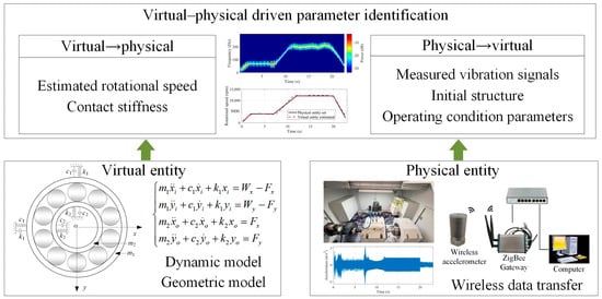
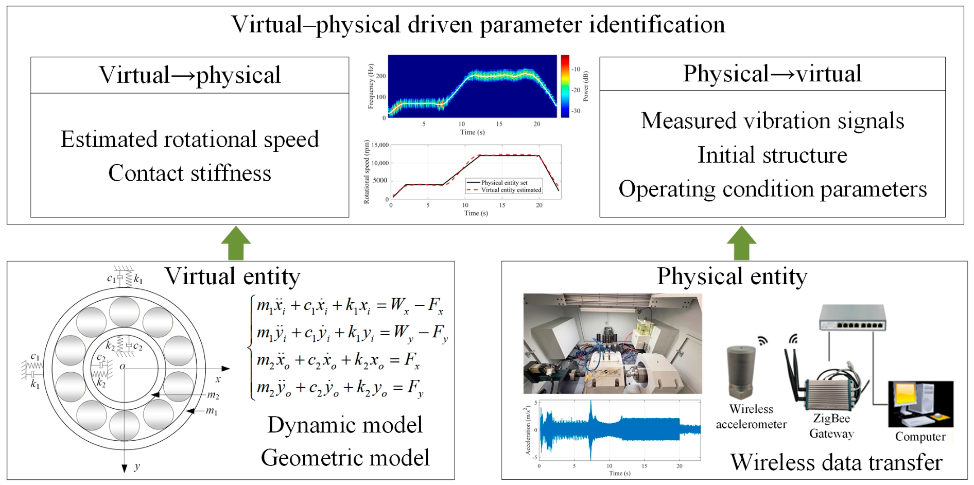
The proposed identification method for the rotational speed and contact stiffness includes three key components: a physical entity, a virtual entity, and parameter identification. Initially, the physical entity is a dedicated experimental test rig capable of simulating the high-speed rotation and rapid start–stop conditions of the EV motor bearings. Subsequently, the virtual entity is constructed based on the bearing geometry and dynamic characteristics to describe its operating behavior. Finally, the rotational speed is extracted from the power spectrum ridgeline of the vibration signals acquired by the wireless accelerometers, and the effective equivalent contact stiffness is inversely identified through optimization using the AFSA by matching the measured and simulated responses. The architecture of the proposed method is shown in Figure 1.
Figure 1.
Architecture of the identification method.
3. Dynamic Model
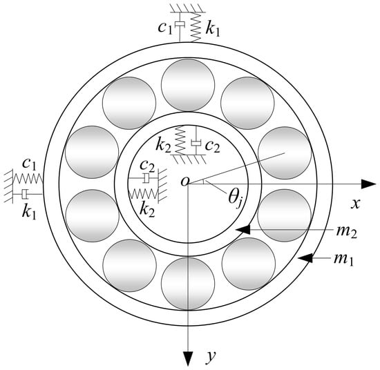
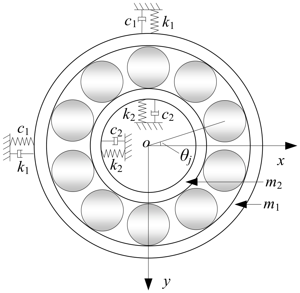
A nonlinear dynamic model is established for the bearing–shaft–housing system to compute key state variables such as the bearing vibration response, characteristic frequency evolution, and equivalent contact stiffness, providing a physical basis for subsequent physical–virtual interactions. The dynamic model consists of an inner ring shaft, outer ring housing, and rolling element contact interfaces, forming a complex nonlinear dynamic system. The dynamic model of the bearing system is established based on the following assumptions [17,18]: (1) The bearing system motion is confined to the radial plane, and the axial and tilting degrees of freedom are neglected. (2) The inner and outer rings are rigidly connected to the shaft and bearing housing, respectively. (3) The contact between the rolling elements and the inner and outer rings follows the Hertzian nonlinear contact theory. (4) The bearing radial clearance is constant. Based on these assumptions, a schematic of the rolling element bearing system model with four DOF is shown in Figure 2.
Figure 2.
Four-degree-of-freedom dynamic model of bearings.
Regarding the assumption of motion confined to the radial plane, six-DOF models include axial dynamics but are computationally heavy, and two-DOF models lack sufficient accuracy. The four-DOF model represents an optimal balance that retains the essential nonlinear Hertzian contact mechanics and radial vibration characteristics while ensuring sufficient computational efficiency for continuous parameter identification. Regarding the assumption of a rigid shaft and housing, the focus of this study is on the internal dynamic evolution of the bearing itself. Neglecting the elastic deformation of external structures reduces the model order. Although this simplification makes the model less sensitive to certain structural resonances, such as pedestal modes, the four-DOF dynamic model adequately captures the characteristic frequencies of the bearing.
The rotational speed is defined as a continuous function of time, , to represent the actual operating conditions of electric drive motor bearings. The angular velocities of the shaft, cage, and rolling elements are obtained as follows:
where N(t) is the instantaneous rotational speed of the shaft; ω(t) is the shaft angular velocity; ωb(t) is the ball angular velocity; ωc(t) is the cage angular velocity; D = 9.525 mm is the ball diameter; and Dm = 46 mm is the pitch diameter.
3.1. Rolling Element Contact Modeling
Contact forces between the rolling elements and inner and outer rings are described using the Hertzian nonlinear contact model. For the j-th rolling element, radial contact deformation can be expressed as follows:
where (xi, yi) and (xo, yo) represent the radial displacements of the inner and outer rings, respectively, θj denotes the instantaneous angular position of the j-th rolling element, δ0 denotes the bearing radial clearance, and Hj(t) indicates the additional displacement caused by a local defect. When contact deformation is positive, the rolling element produces Hertzian nonlinear contact force as follows:
where kb is the equivalent Hertzian contact stiffness coefficient and δj is the radial contact deformation. It should be noted that this stiffness is defined as the ratio of instantaneous radial force to displacement. While this simplification facilitates parameter identification, it may exhibit increased variability under variable load conditions if rolling element inertia and lubrication film effects become significant.
For bearings with local defects, the additional displacement Hj(t) represents the loss of contact material when the rolling element passes through the defect region. In this study, groove defects of specified widths are introduced on the outer or inner raceway using wire electrical discharge machining. For a groove defect with width L, the angular width of the defect region is defined as θd = arcsin(L/Router), and the additional displacement is expressed as:
where dr denotes the defect depth. Similarly, for an inner ring groove defect, the angular width is θd = arcsin(L/Rinner), and the additional displacement is defined as
By decomposing and summing the contact forces of all the rolling elements in the radial plane, the nonlinear support forces provided by the bearing can be obtained. The resulting components in the horizontal and vertical directions are denoted as Fx(t) and Fy(t), respectively.
These support forces act simultaneously on the inner and outer rings through rolling element contacts, forming an action–reaction pair of equal magnitude and opposite direction acting on the inner and outer rings.
3.2. Nonlinear Dynamic Modeling
In this study, a four-degree-of-freedom nonlinear dynamic model is developed for the bearing–shaft–housing system in the radial plane. The corresponding dynamic equations are expressed as follows:
where m1, c1, and k1 as well as m2, c2, and k2 represent the equivalent mass, damping, and stiffness of the inner ring (shaft) and outer ring (housing), respectively, and Wx and Wy denote external loads. The dynamic parameters are set as follows: m1 = 5 kg, m2 = 10 kg, c1 = 1300 Ns/m, c2 = 2200 Ns/m, k1 = 7.42 × 10⁷ N/m, k2 = 1.51 × 10⁷ N/m. It should be noted that the signals in this dynamic modeling are not fully consistent with those of the test rig, and the dynamic parameters including the mass, stiffness, and damping are set as a rule of thumb. As a result, the identified effective equivalent contact stiffness may partially compensate for unmodelled dynamics, damping uncertainty, and structural discrepancies between the model and the physical system. Therefore, the identified stiffness should be interpreted as an effective parameter that reflects both the contact behavior and the model limitations, rather than a purely physical contact stiffness. The computational procedure of the 4-DOF bearing dynamic model is outlined in Algorithm 1.
| Algorithm 1. Computational procedure of the bearing dynamic model |
| 1. Input t, |
| 2. Compute N(t), ω, ωb, ωc, kb |
| 3. Initialize Fx = 0, Fy = 0, |
| 4. For j = 1 to Nb do |
| 5. ; |
| 6. if , then |
| 7. end if |
| 8. end for |
| 9. ; |
| ; |
| 10. Output |
Based on nonlinear support forces, together with the relative radial displacements of the inner and outer rings, the equivalent contact stiffness of the bearing in the radial plane can be further defined. The equivalent contact stiffness is defined as the ratio of the instantaneous radial contact force to the relative radial displacement between the inner and outer rings. This stiffness exhibits significant time-varying characteristics as it evolves with the rotation speed, load distribution, and local defects as follows:
4. Parameter Identification Method
4.1. Inverse Update of Effective Equivalent Contact Stiffness
An inverse identification of the effective equivalent contact stiffness of the bearing is performed to ensure consistency between the vibration responses of the virtual and physical entities. This approach does not directly modify the dynamic model structure or material parameters; instead, it indirectly adjusts the contact stiffness by imposing consistency constraints on the vibration response.
The inverse problem aims to minimize the difference between the virtual (dynamic model trial results) and the physical (experimental results) entities. To minimize this error, the root mean square error (RMSE) of the measured and simulated signals in the frequency domain is used as the objective function.
where K represents the trial parameter and gmea,i and gsim,i represent the discrete Fourier transform values of the measured and simulated vibration signals at the i-th frequency point, respectively.
Because the equivalent contact stiffness is not explicitly included as a state parameter in the governing dynamic equations and the Hertzian contact stiffness coefficient plays a dominant role in the contact force formulation, a stiffness scaling factor η = K/Kref is introduced, where Kref is the reference equivalent contact stiffness under the baseline operating condition. The dynamic model is updated by scaling the Hertzian contact stiffness coefficient, and the effective contact stiffness coefficient is defined as kb = ηkb,nom, where kb,nom is the nominal contact stiffness coefficient, determined by the material parameters and contact geometry, and kb represents the effective Hertzian contact stiffness coefficient employed in the dynamic model.
4.2. Optimization Algorithm
To solve the aforementioned inverse problem, an optimization algorithm must be adopted to minimize the objective function in Equation (9) to find the optimal values for the trial parameter K. In this study, the AFSA [19] is used for optimization. According to a test comparison conducted by Pourpanah et al. [20], the AFSA exhibits superior stability compared to the particle swarm optimization (PSO), fewer algorithmic parameters compared to the differential evolution (DE) algorithm, consistent performance across all functions compared to the firefly algorithm (FA), and balanced convergence behavior compared to the grey wolf optimizer (GWO) and cuckoo search algorithm (CSA). The AFSA simulates the foraging behavior of fish in a swarm, where each artificial fish represents a potential solution Ki, and its movements are guided by three behaviors: prey behavior, swarm behavior, and follow behavior. Fish search for better solutions by adjusting their positions based on the fitness of neighboring fish, ultimately converging toward an optimal value.
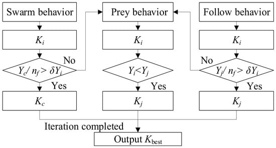
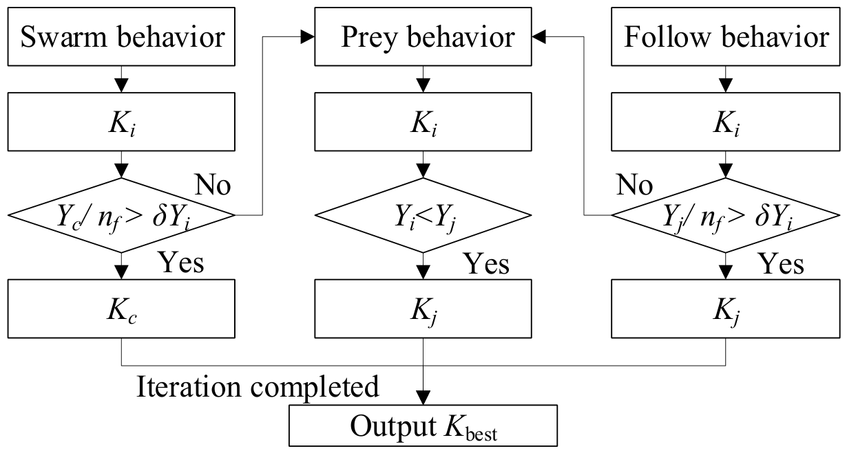
Figure 3 illustrates the basic flowchart of the AFSA simulation procedure. For the follow behavior, the fish moves toward the best neighboring position Kj if Yj/nf > δYi is satisfied, where Yj is the food concentration at the best companion position, nf is the number of companions within the visual distance, and δ is the crowding factor. The fish attempts the swarm behavior, moving toward the swarm center Kc if Yc/nf > δYi is satisfied, where Yc is the food concentration at the center position. If neither condition is satisfied, the fish performs the prey behavior, randomly searching for a better position within its visual distance and moving toward Kj if Yi < Yj is met. After each behavior is executed, the fish updates its position, and the iteration continues until the maximum iteration number is reached. Finally, the optimal solution Kbest recorded on the bulletin board is output as the identified result.
Figure 3.
Flowchart of the artificial fish swarm algorithm (AFSA).
The AFSA randomly generates the initial fish swarm positions before the aforementioned three behaviors. A logistic chaotic sequence model is used to establish the initial swarm. This model generates the chaotic variables according to the following equations:
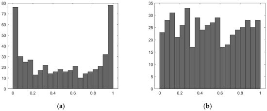
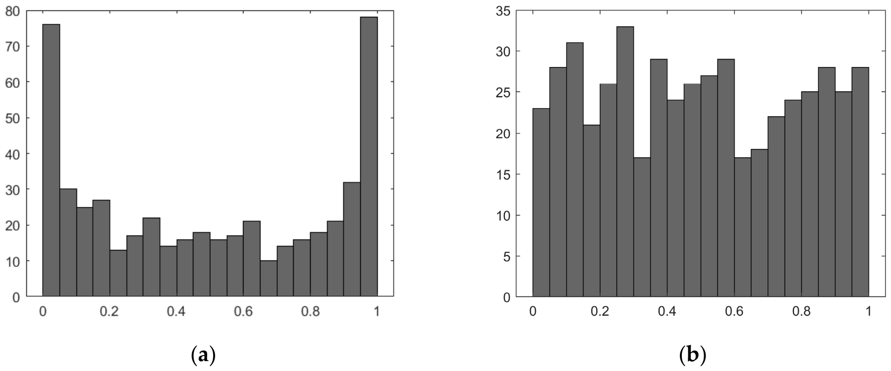
where 0 ≤ μ ≤ 4 is the Lyapunov exponent [21]. Research on chaotic dynamical systems indicates that when 3.5699457 ≤ μ ≤ 4, the logistic mapping exhibits chaotic behavior. However, the raw positions obtained from the basic logistic chaotic sequence are not uniform, as shown in Figure 4a, making them unsuitable for AFSA. Therefore, the transformation of the nonuniformly distributed random variables into uniformly distributed random variables, as shown in Figure 4b, is performed using
Figure 4.
Frequency distribution map of the logistic chaotic sequences: (a) uneven distribution, (b) uniform distribution.
The parameters in the AFSA are set as follows: the swarm size is 20, the maximum number of iterations is 15, the visual distance is 0.5, the step size is 0.01, and the crowding factor δ is 1.68.
4.3. Energy Ridge Tracking for Rotational Speed Estimation
To obtain the real-time rotational speed of the electric drive motor bearing from the nonstationary vibration signal of the experimental test rig, a time–frequency energy ridge-tracking method is employed to extract the bearing fault frequency. Initially, the demeaned raw vibration signal a(t) is input into the short-time Fourier transform (STFT) with a Hamming window of 0.5 s, 90% overlap, and 8192 FFT points, yielding a frequency resolution of 1.22 Hz and a time resolution of 0.05 s:
where w is the window function, τ is the integration variable, and t denotes time. The resulting power spectrum is given by
The spectrogram is analyzed over the frequency band of 0–300 Hz. For each time slice tk, the maximum energy point along the frequency axis of the power spectrum is identified, forming a time–frequency energy ridge.
To avoid ridge misclassification caused by the dominance of the second harmonics, a narrow-band search strategy is adopted:
where f0(tk) is the theoretical shaft frequency determined from the five-condition speed profile and = 10 Hz is the half bandwidth of the search window. The instantaneous rotational speed was estimated to be N(tk) = 60fr(tk). It should be noted that the narrowband search strategy relies on a preset theoretical shaft frequency range, which may be limited in scenarios with abrupt speed changes or unknown operating conditions.
5. Experimental Results and Discussion
5.1. Experimental Setup
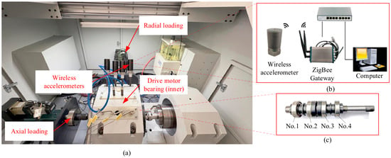
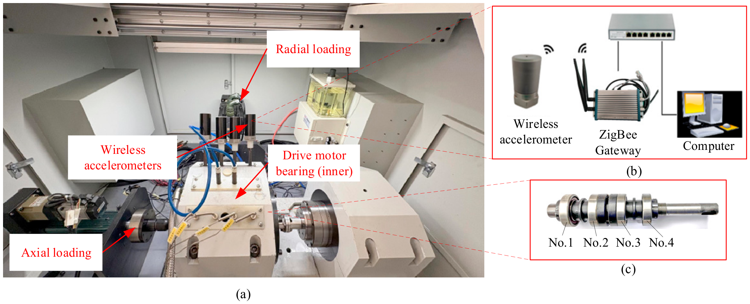
The bearing test rig, illustrated in Figure 5, consists of four 6206 deep-groove ball bearings used for electric vehicle applications: two test bearings (Nos. 1 and 4) and two supporting bearings (Nos. 2 and 3), as shown in Figure 5c. The radial load range is 200 N–20 kN and the axial load range is 50 N–10 kN. Two independent servo electric cylinders are employed for radial and axial load application, respectively, each with its own force sensor and servo motor to enable precise closed-loop control of loading speed, displacement, and force. The bearing is driven by a synchronous electric spindle at a rotational speed of 2000–45,000 rpm. It features a rapid speed change response with a maximum acceleration rate of 10,000 rpm/s. These characteristics ensure that the experimental setup is suitable for high-speed operation and frequent start–stop conditions of electric vehicle drive motor bearings. Vibration signals are measured on the bearing outer ring using wireless accelerometers, with a sampling frequency of 10 kHz in the range of ±50 g, as shown in Figure 5b. The measurement accuracy is higher than ±5%. The measurement system comprised four DH5975W wireless accelerometers and one DH5609-3A gateway that communicate wirelessly through ZigBee. The gateway is connected to a switch and communicates with a computer.
Figure 5.
Drive motor bearing test system for electric vehicles: (a) experimental setup, (b) wireless data transmission, and (c) bearings mounting positions.
5.2. Interaction Loop
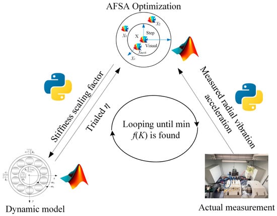
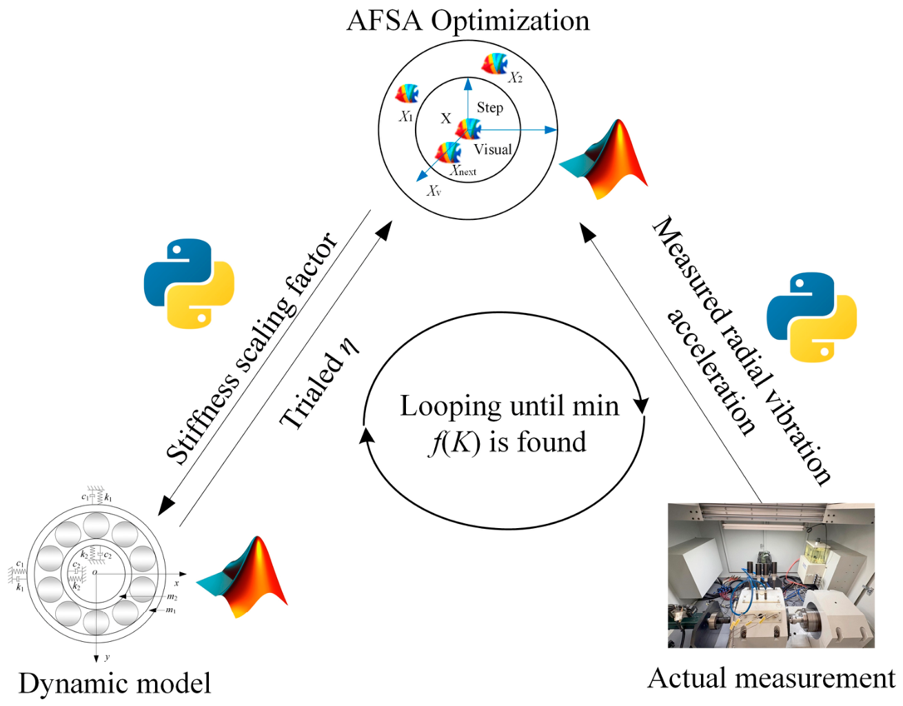
The interaction loop integrating the physical measurement, AFSA optimization, and dynamic model is implemented using a MATLAB-PYTHON framework, as shown in Figure 6. The experimental test rig transmits vibration signals via the wireless accelerometers, from which the rotational speed and radial vibration acceleration are extracted as the measurement inputs. MATLAB software is used to execute the dynamic simulation and run the AFSA optimization iterations to generate the stiffness scaling factor. The PYTHON script serves as the data exchange layer. At each optimization cycle, it reads the trial stiffness scaling factor η generated by the AFSA, writes it to a text file, and calls the MATLAB dynamic model, where η scales the Hertzian contact stiffness coefficient as kb = ηkb,nom. After the MATLAB simulation completes, PYTHON reads the simulated acceleration from the output file, computes the RMSE according to Equation (9) and feeds it back to the AFSA to update η. The interaction loop is performed on a computer with an Intel Core i5-14600KF CPU @ 3.50 GHz and 32 GB of RAM, using MATLAB version 2020a and Python 3.8.
Figure 6.
Workflow of the interaction loop between the physical and virtual entities.
The computational latency of the effective equivalent contact stiffness identification is approximately 20–30 s per update cycle, consisting of AFSA iterations and corresponding dynamic model simulations. The computational latency for rotational speed estimation is approximately 0.15 s, which includes data acquisition, wireless transmission, and energy ridge extraction. The effective equivalent contact stiffness is updated approximately once every 20–30 s, whereas the rotational speed is updated 6–7 times/s. This update rate reflects a delayed sequential parameter identification process.
5.3. Experimental Results
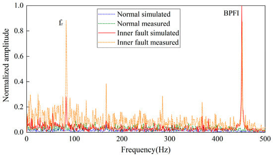
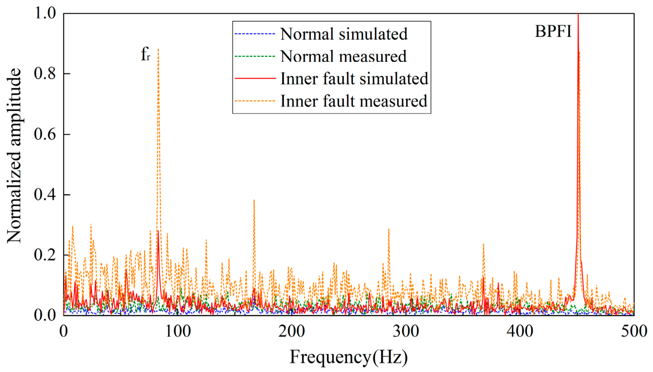
Test cases were conducted for both healthy and faulty bearings. Envelope spectrum analysis under both conditions was first conducted, as shown in Figure 7. The healthy bearing was tested at 10,000 rpm and the inner-race fault bearing at 5000 rpm. The time-domain signal was recorded for a duration of 1 s, and the envelope spectrum was displayed over a frequency range of 0–500 Hz. It can be seen from Figure 7 that, for the healthy state, both the simulated and measured envelope spectra are flat with low baseline amplitudes and no prominent periodic peaks. In contrast, under the inner race fault condition, distinct peaks appear at the ball pass frequency of the inner race (BPFI, 450 Hz) and the shaft rotating frequency (fr, 83 Hz), which are consistent with the theoretical [22] calculations, and close agreement is also observed between simulated and measured peak locations. Under the tested conditions, the envelope spectra show no obvious sidebands, broadband excitation, or other features indicative of modal coupling and nonlinear resonance.
Figure 7.
Envelope spectrum comparison.
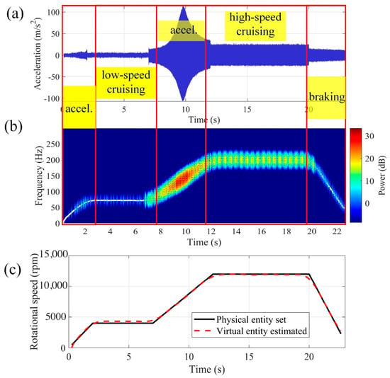
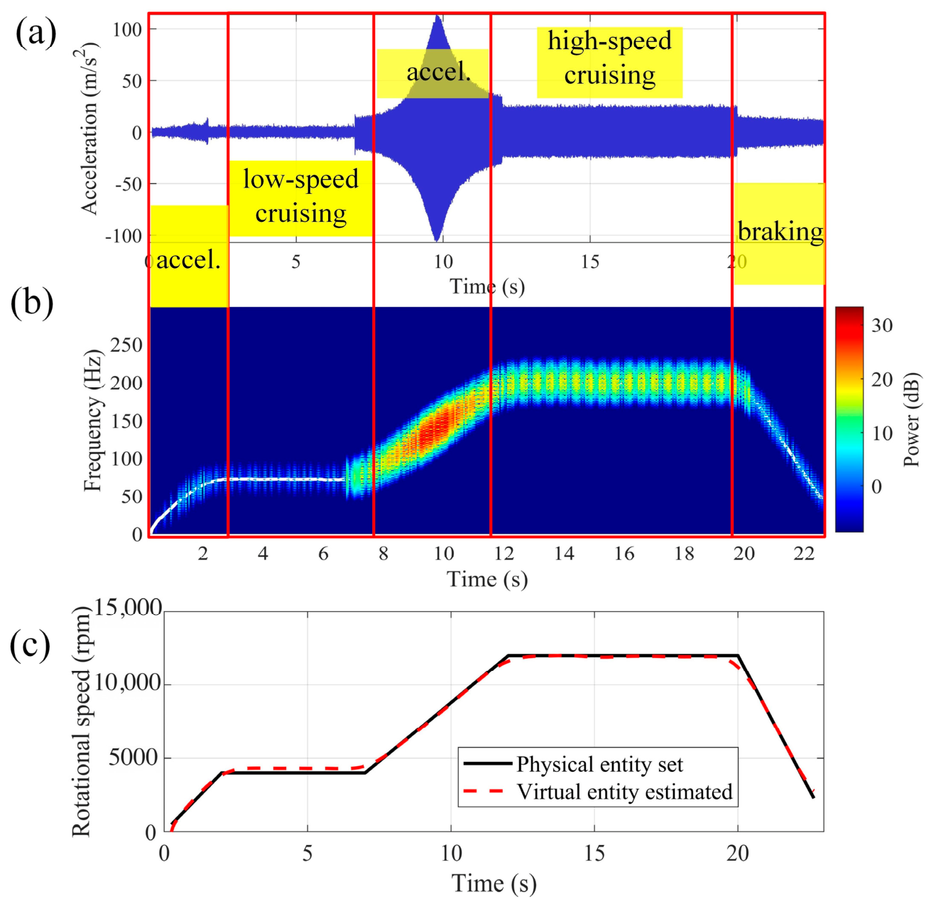
For the healthy bearing, the bearing test rig is set to operate under five conditions: the system accelerates from 0 to 4000 rpm in 0–2 s, maintains low-speed cruising between 2–7 s, accelerates to the maximum rpm in the interval 7–12 s, functions in high-speed cruising in the interval 12–20 s, and decelerates during the braking phase, that is, from 20 to 23 s. Three radial loads of 1000 N, 3000 N, and 5000 N and three maximum rotational speeds of 8000 rpm, 10,000 rpm, and 12,000 rpm were selected, resulting in nine test scenarios. For the healthy bearings, the local defect term Hj(t) in the dynamic model is set to zero. The ground truth for rotational speed validation is the real-time controller-reported speed from the spindle servo system. The estimation performance for rotational speed for each condition is listed in Table 1, Table 2 and Table 3.
Table 1.
Estimation performance for the rotational speed under 1000 N.
Table 2.
Estimation performance for the rotational speed under 3000 N.
Table 3.
Estimation performance for the rotational speed under 5000 N.
It can be seen that for each load condition, the mean absolute errors range from 99 rpm to 158 rpm, 125 rpm to 131 rpm, and 124 rpm to 145 rpm for loads of 1000 N, 3000 N, and 5000 N, respectively. The mean relative errors ranged from 1.83% to 2.76%, 2.40% to 2.57%, and 2.68% to 2.92%, respectively. At 3000 N, the errors at 8000 rpm, 10,000 rpm, and 12,000 rpm are 2.56%, 2.57%, and 2.40%, respectively, showing minimal variation despite a 50% increase in rotational speed. At 12,000 rpm, the errors for loads of 1000 N, 3000 N, and 5000 N are 2.22%, 2.40%, and 2.75%, respectively, indicating only a modest increase with the load. Across all conditions, the mean absolute error and root mean square error remained stable, and the relative error remained below 3%. A mean relative error of 1.83% to 2.92% corresponds to an absolute speed deviation of approximately 99–198 rpm across the tested range of 8000–12,000 rpm. A mean relative error within 3% is acceptable for EV bearing monitoring. The rotational speed determines the bearing characteristic frequencies, and a 3% deviation introduces a proportional frequency shift that remains within the typical frequency resolution for vibration analysis without affecting the reliable identification of spectral features for condition assessment.
The results corresponding to a maximum rotational speed of 12,000 rpm and a radial load of 5000 N are shown in Figure 8. Figure 8a–c show the time-domain acceleration response, time–frequency power spectrum with an energy ridge, and speed estimation comparison, respectively. As shown in Figure 8a, the vibration amplitude remains low during startup and low-speed cruising, increases significantly during acceleration, reaches its peak during high-speed cruising, and attenuates during braking. These distinct characteristics reflect the strong influence of rotational speed on the dynamic response of the bearing under heavy radial loading. As shown in Figure 8b, the extracted energy ridge clearly captures the dominant frequency component and exhibits a continuous and smooth evolution over time. The ridge frequency increases monotonically during acceleration, remains stable during cruising, and decreases monotonically during deceleration, indicating the effective tracking of time-varying rotational behavior under nonstationary conditions. Figure 8c confirms the close agreement between the estimated and set rotational speeds, with a mean relative error of 2.75% for this condition, as shown in Table 3.
Figure 8.
Estimation of rotational speed of EV motor bearing: (a) time-domain acceleration, (b) power spectrum ridge, and (c) rotational speed comparison.
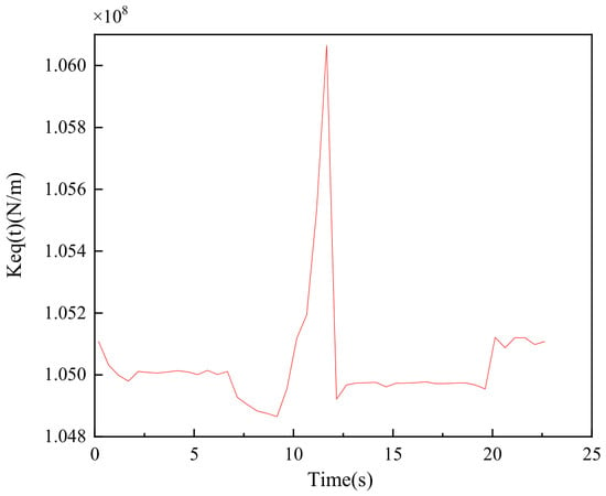
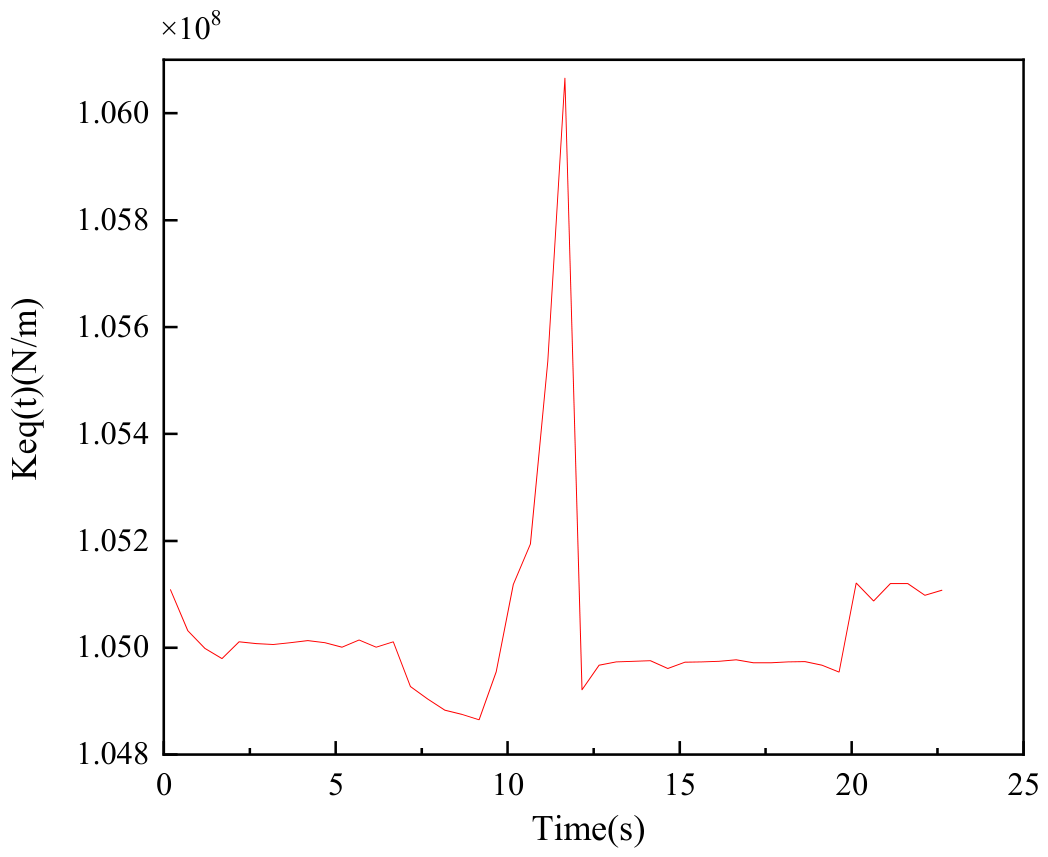
The evolution of the identified effective equivalent contact stiffness for a maximum rotational speed of 12,000 rpm and a radial load of 5000 N is shown in Figure 9. These effective stiffness parameters were obtained through delayed sequential updates during the experiment. It can be seen that the stiffness exhibits distinct stage-dependent characteristics, with notable fluctuation during the acceleration phases and relative stabilization during cruising intervals. This evolution is physically consistent because the equivalent contact stiffness is governed by nonlinear Hertzian contact mechanics, which dynamically reconfigure with the rotational speed under heavy radial loading.
Figure 9.
Effective stiffness parameter obtained through inverse model updating for a maximum rotation speed of 12,000 rpm and load of 5000 N.
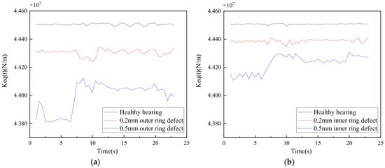
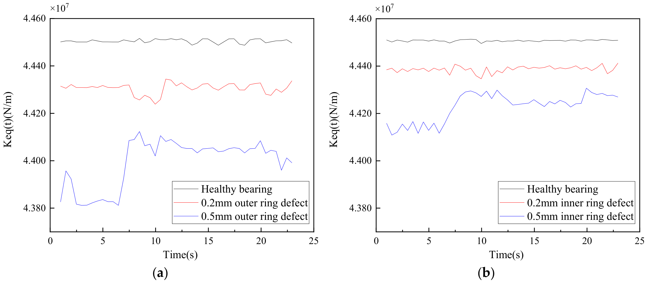
Test cases under different fault conditions were further conducted, including outer ring groove defects of widths 0.2 mm and 0.5 mm at a depth of 0.3 mm, and inner ring groove defects with the same dimensions. Owing to these defects, the maximum rotational speed was limited to 5000 rpm and the radial load was set to 500 N to prevent catastrophic failure during the test. Figure 10 shows the evolution of the identified effective equivalent contact stiffness. Figure 10a presents the results for the outer ring defects and Figure 10b presents the results for the inner ring defects. The healthy bearing exhibits the highest stiffness of approximately 4.45 × 10⁷ N/m, while the 0.2 mm and 0.5 mm defect bearings show progressively lower stiffness. Under this moderate-speed and light-load condition, the contact deformation remains small, and the bearing operates in an approximately linear regime; therefore, the stiffness curves do not exhibit pronounced stage-dependent fluctuations. This trend is physically consistent, because larger defects reduce the effective contact area. The stiffness reduction is more pronounced for the outer ring defects, which can be attributed to the higher contact stresses experienced by the outer raceway under radial loading.
Figure 10.
Effective stiffness parameter obtained through inverse model updating: (a) outer ring defect and (b) inner ring defect.
6. Conclusions
In this study, we developed an identification method to estimate the rotational speed and contact stiffness of EV motor bearings. A dynamic model of the bearings incorporating nonlinear Hertzian contact and variable-speed conditions was established as the virtual entity, and the physical entity was established as an EV motor-bearing test rig equipped with wireless accelerometers and ZigBee data transmission for acquisition of vibration. The effective equivalent contact stiffness was determined by combining physical measurements, virtual simulations, and optimization using AFSA. The rotational speed was estimated with a mean relative error of <3% across varying loads and speeds. The effective equivalent contact stiffness was identified, exhibiting a stage-dependent evolution under dynamic conditions.
Future work can extend the virtual entity to incorporate rolling element inertia and lubrication film effects. Additionally, deep learning models can be trained to map virtual entity outputs to high-fidelity simulated data that match physical signals, further improving physical consistency.
Author Contributions
Conceptualization, H.Y. and Y.X.; methodology, H.Y.; software, Z.M.; validation, H.C., J.Y. and H.D.; investigation, F.P.; writing—original draft preparation, H.Y.; writing—review and editing, Y.X. and H.C.; supervision, Y.X. All authors have read and agreed to the published version of the manuscript.
Funding
The authors are thankful for the support from the University-Enterprise Collaborative Innovation Program of Henan Province (No. 26AXQXT025) and Postdoctoral Fellowship Program of CPSF (No. GZC20250944).
Data Availability Statement
The original contributions presented in this study are included in the article. Further inquiries can be directed to the corresponding author.
Conflicts of Interest
Author Ziteng Mi was employed by the company Beijing Drainage Group Co., Ltd., authors Honglin Du and Fengya Pang were employed by the company Luoyang Kaiyuan Intelligent Precision Machinery Co., Ltd. The remaining authors declare that the research was conducted in the absence of any commercial or financial relationships that could be construed as a potential conflict of interest.
References
- Zhang, X.; Hu, Y.; Gong, C.; Deng, J.; Wang, G. Artificial intelligence technique-based EV powertrain condition monitoring and fault diagnosis: A review. IEEE Sens. J. 2023, 23, 16481–16500. [Google Scholar] [CrossRef] [Scilit]
- Wang, F.; Wang, X.; Yang, T.; Bai, X.; Zhang, Q.; Wu, Z. Interpretable fault diagnosis of rolling bearings: The BISR-Former framework for complex operational regimes. Phys. Scr. 2025, 100, 116006. [Google Scholar] [CrossRef] [Scilit]
- Liu, S.; Lv, J.; Yang, Z.; Kuang, L.; Zhao, L.; Liu, C. The discharge characteristics and damages in the EV motor bearings: Influenced by the rotational speeds and lubricating oil viscosities. Wear 2025, 205, 205863. [Google Scholar]
- Lu, S.; Yan, R.; Liu, Y.; Wang, Q. Tacholess speed estimation in order tracking: A review with application to rotating machine fault diagnosis. IEEE Trans. Instrum. Meas. 2019, 68, 2315–2332. [Google Scholar] [CrossRef] [Scilit]
- Cosenza, C.; Malfi, P.; Melluso, F.; Nicolella, A.; Niola, V. A virtual sensor for wheel angular speed estimation: Application on a differential drive wheeled robot. J. Intell. Robot. Syst. 2025, 111, 117. [Google Scholar] [CrossRef] [Scilit]
- Li, H.; Liu, T.; Wu, X.; Chen, Q. An optimized VMD method and its applications in bearing fault diagnosis. Measurement 2020, 166, 108185. [Google Scholar] [CrossRef] [Scilit]
- Pavithra, R.; Ramachandran, P. Non-stationary signal analysis utilizing VMD and EMD algorithm for multiple fault classification for industrial applications. J. Intell. Fuzzy Syst. 2025, 49, 291–309. [Google Scholar]
- Sowmya, S.; Saimurugan, M.; Venkatesh, N. Distinctive contribution of sound spectral features in enhancing vibration-based multi-component fault classification under non-stationary speed conditions. IEEE Access 2025, 13, 126261–126278. [Google Scholar]
- Wang, X.; Lu, S.; Chen, K.; Wang, Q.; Zhang, S. Bearing fault diagnosis of switched reluctance motor in electric vehicle powertrain via multisensor data fusion. IEEE Trans. Ind. Inf. 2021, 18, 2452–2464. [Google Scholar] [CrossRef] [Scilit]
- Cao, Z.; Wu, G.; He, C.; Rao, M.; Tu, W. A new instantaneous contact based dynamic model of rolling element bearings with local defects. Mech. Syst. Signal Process. 2023, 200, 110600. [Google Scholar] [CrossRef] [Scilit]
- Zhao, Z.; Sun, S.; Xu, W.; Shen, C.; Wang, D. Dynamics modeling and fault diagnosis of flexible thin-walled elliptical bearings in harmonic reducers. Measurement 2024, 238, 115378. [Google Scholar] [CrossRef] [Scilit]
- He, P.; Wang, Y.; Liu, H.; Guo, E.; Wang, H. Optimization design of structural parameters of single-row four-point contact ball slewing bearing. J. Braz. Soc. Mech. Sci. Eng. 2020, 42, 291. [Google Scholar]
- Chen, R.; Li, J.; Wang, Y.; Deng, R.; Chen, W.; Li, W. Study on the time-varying stiffness characteristics of four-point contact ball bearings. Lubricants 2025, 13, 118. [Google Scholar]
- Halpin, J.D.; Tran, A.N. An analytical model of four-point contact rolling element ball bearings. J. Tribol. 2016, 138, 031404. [Google Scholar] [CrossRef] [Scilit]
- Chen, C.; Zhang, L.; Hua, C.; Liu, Z.; Meng, Q.; Shi, J. Research on Online Non-Contact Test Device and Test Method for Bearing Stiffness of Electric Spindle. Machines 2025, 13, 516. [Google Scholar] [CrossRef] [Scilit]
- Song, W.; Guo, L.; Yu, Y.; Gao, H.; Xu, H.; Feng, T. A parameter-interactive digital twin model of bearings under variable speeds. Measurement 2025, 244, 116307. [Google Scholar]
- Dong, Y.; Li, Y.; Zheng, H.; Wang, R.; Xu, M. A new dynamic model and transfer learning based intelligent fault diagnosis framework for rolling element bearings race faults: Solving the small sample problem. ISA Trans. 2022, 121, 327–348. [Google Scholar] [CrossRef] [Scilit] [PubMed]
- Cui, L.; Zhang, Y.; Zhang, F.; Zhang, J.; Lee, S. Vibration response mechanism of faulty outer race rolling element bearings for quantitative analysis. J. Sound Vib. 2016, 364, 67–76. [Google Scholar] [CrossRef] [Scilit]
- Neshat, M.; Sepidnam, G.; Sargolzaei, M.; Toosi, A.N. Artificial fish swarm algorithm: A survey of the state-of-the-art, hybridization, combinatorial and indicative applications. Artif. Intell. Rev. 2014, 42, 965–997. [Google Scholar]
- Pourpanah, F.; Wang, R.; Lim, C.P.; Wang, X.-Z.; Yazdani, D. A review of artificial fish swarm algorithms: Recent advances and applications. Artif. Intell. Rev. 2023, 56, 1867–1903. [Google Scholar]
- Zhang, Y.P.; Duan, F.; Liu, X. The research of applying chaos theory to speech communicating encryption system. Adv. Multimed. Softw. Eng. Comput. 2012, 2, 197–202. [Google Scholar]
- Ng, S.S.Y.; Tse, P.W.; Tsui, K.L. A one-versus-all class binarization strategy for bearing diagnostics of concurrent defects. Sensors 2014, 14, 1295–1321. [Google Scholar] [PubMed]

Disclaimer/Publisher’s Note: The statements, opinions and data contained in all publications are solely those of the individual author(s) and contributor(s) and not of MDPI and/or the editor(s). MDPI and/or the editor(s) disclaim responsibility for any injury to people or property resulting from any ideas, methods, instructions or products referred to in the content. |
© 2026 by the authors. Licensee MDPI, Basel, Switzerland. This article is an open access article distributed under the terms and conditions of the Creative Commons Attribution (CC BY) license.