


Abstract
Pressure pulsations generated by pumps impair noise behaviour, increase mechanical loading, and reduce control performance in hydraulic systems. This study investigates the use of a rotary mechanical pulsation compensator integrated into the drivetrain of an external gear pump. The aim is to attenuate pulsations directly at their source without modifying the hydraulic layout. This is accomplished by using the torque induced flow rate pulsation to cancel the external flow rate excitation, which leads to destructive interference between flow rate induced and torque induced pressure pulsations. An analytical frequency domain model of the coupled mechanical–hydraulic system is derived to determine the required stiffness and damping conditions. The theoretical results are validated experimentally at mean pressure levels of 100 bar and 170 bar, both for two different hydraulic layouts. With a resonator pipeline at the pump outlet, the first harmonic of the pressure pulsation at the compensation frequency is reduced by 10.9 bar and 18.4 bar, respectively, which corresponds to reduction rates of 93% and 98%. The required damping value depends on the operating conditions, but it is independent of the hydraulic layout. While insufficient damping increases pressure pulsations around the compensation frequency, slightly higher damping flattens the frequency characteristics of pressure pulsation and reduces the maxima around the compensation frequency. In the neighbourhood of this frequency, the proposed concept enables effective reduction of the first pressure pulsation harmonic through a structural modification of the drivetrain.
1. Introduction
Pressure pulsations in hydraulic systems are primarily caused by periodic variations of pump or motor flow rate and constitute a major source of noise emissions. Hydraulic pressure transients are typically associated with valve dynamics or external excitations. Both pressure transients and pulsations result in mechanical loads and challenge the layout of motion control [1].
Flow rate variations can be reduced by constructive design measures, such as increasing the number of pistons in piston machines or optimising the tooth geometry in gear pumps [2,3]. However, these measures increase structural and design complexity. As a consequence, a wide range of approaches has been developed to attenuate pressure pulsations through targeted modifications of the hydraulic system. These approaches can generally be classified into passive and active systems.
In [4,5], active control strategies based on external flow rate excitation are proposed to suppress pressure pulsations in hydraulic pipelines. Both approaches demonstrate effective attenuation in experimental investigations. Active pulsation attenuators offer flexible adaptation to different operating conditions and operate over a wide frequency range. However, they require dedicated measurement systems, real-time capable controllers, and fast-response actuators. As a result, system complexity is increased, which leads to reduced overall reliability and increased costs [6].
Passive solutions are characterised by a simple design and can generally be classified into resistive and reactive approaches. Resistive damping attenuators, such as orifices, provide attenuation over a wide frequency range but cause considerable energy dissipation and increased heat generation [6].
A well-known reactive solution is the Helmholtz resonator, which consists of hydraulic inductance and capacitance. It enables targeted compensation at a specific frequency. To achieve a broader attenuation bandwidth, Helmholtz resonators can be extended to multi-degree-of-freedom systems, which increases overall system complexity [7]. Furthermore, adaptive implementations have been investigated. For example, Ref. [8] describes a resonator with adjustable capacitance, allowing the natural frequency to be adapted to current operating conditions. Another reactive passive solution is the branch damper [9], which is based on quarter-wavelength (/4) resonance and consists of a laterally connected branch line. For typical pump pulsation frequencies, the required installation space is a significant drawback of both Helmholtz resonator and branch damper.
A mechanical pulsation compensator designed in analogy to a Helmholtz resonator is investigated in [10]. The compensator reduces installation space by implementation as a spring–mass oscillator with a hydraulic spring, whose natural frequency can be adjusted by varying the enclosed hydraulic volume. All these approaches require integration into the hydraulic system.
To avoid the spread of pulsations in the hydraulic system, it is advisable to reduce pressure pulsations as close as possible to their point of origin. For positive displacement pumps, two options exist to achieve this without modifying the pump itself: directly at the pump outlet or at the pump shaft. The attachment of hydraulic devices always requires a certain distance between the attachment point and the pump outlet. Therefore, a rotary mechanical pulsation compensator was developed to compensate pressure pulsations at the pump shaft as described in [11]. This device transforms the pump drivetrain into an oscillating system that interacts with the hydraulic system via the pump.
The drivetrain, which is analysed in detail in [12], includes the mass moment of inertia of the motor side, the mass moment of inertia of the pump side, and a torsional compliance in between. This assembly corresponds to an unconstrained two-mass torsional oscillator. Due to the significantly higher inertia on the motor side, it can be approximated as a constrained single-mass torsional oscillator.
The resulting single-degree-of-freedom system is analogous to a Helmholtz resonator, where the torsional compliance corresponds to the hydraulic capacitance, and the mass moment of inertia of the pump side corresponds to the hydraulic inductance. In [13], a design method for the torsional compliance, also referred to as the compensator coupling, is presented. First experimental investigations of the rotary mechanical pulsation compensator with a radial piston pump are reported in [14]. Although a compensation effect was demonstrated, the attenuation bandwidth proved to be very narrow for this pump type.
Further investigations of the rotary mechanical compensator, including calculations and measurements with internal gear pumps, are presented in [15]. These results indicate significantly improved compensation performance. Even though the same compensator as in [14] was used, a much broader attenuation effect was observed, which could be attributed to the lower mass moment of inertia of the internal gear pump.
The type of pulsation plays a crucial role when applying a drivetrain with reduced torsional compliance. In [15], investigations with an internal gear pump distinguish the influence of kinematic and dynamic pulsations and their impact on the periodic flow rate and torque variations. A detailed description of kinematic and dynamic pulsation mechanisms is given in [16].
In this paper, the rotary mechanical pulsation compensator is investigated in combination with external gear pumps. Such pumps are widely applied and generate pronounced pulsations. Due to the dominant kinematic pulsation component [17], the rotary mechanical pulsation compensator also responds to torque variations and cannot be used in its previous form. It is shown how the compensation effect can benefit from kinematic pulsations in combination with a tuned, damped torsional oscillator in the pump drivetrain. For this purpose, the coupling from [14] is supplemented by additional damping. Beyond the previous compensation effect, the compensator adjusts the pressure pulsations caused by periodic torque variations in order to counteract the pressure pulsations caused by periodic flow rate variations [18]. It is demonstrated that the first harmonics of these pulsations cancel each other in one particular operating point.
2. Analytical Investigation of Pulsation Cancellation
2.1. Model of an External Gear Pump for Analytical Frequency Domain Investigation
Due to the kinematics of the pump, the instantaneous displacement depends on the angular position . A derivation of the corresponding relationship is given in [2]. The flow rate is expressed as
where denotes the angular velocity. The corresponding torque is given by
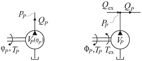
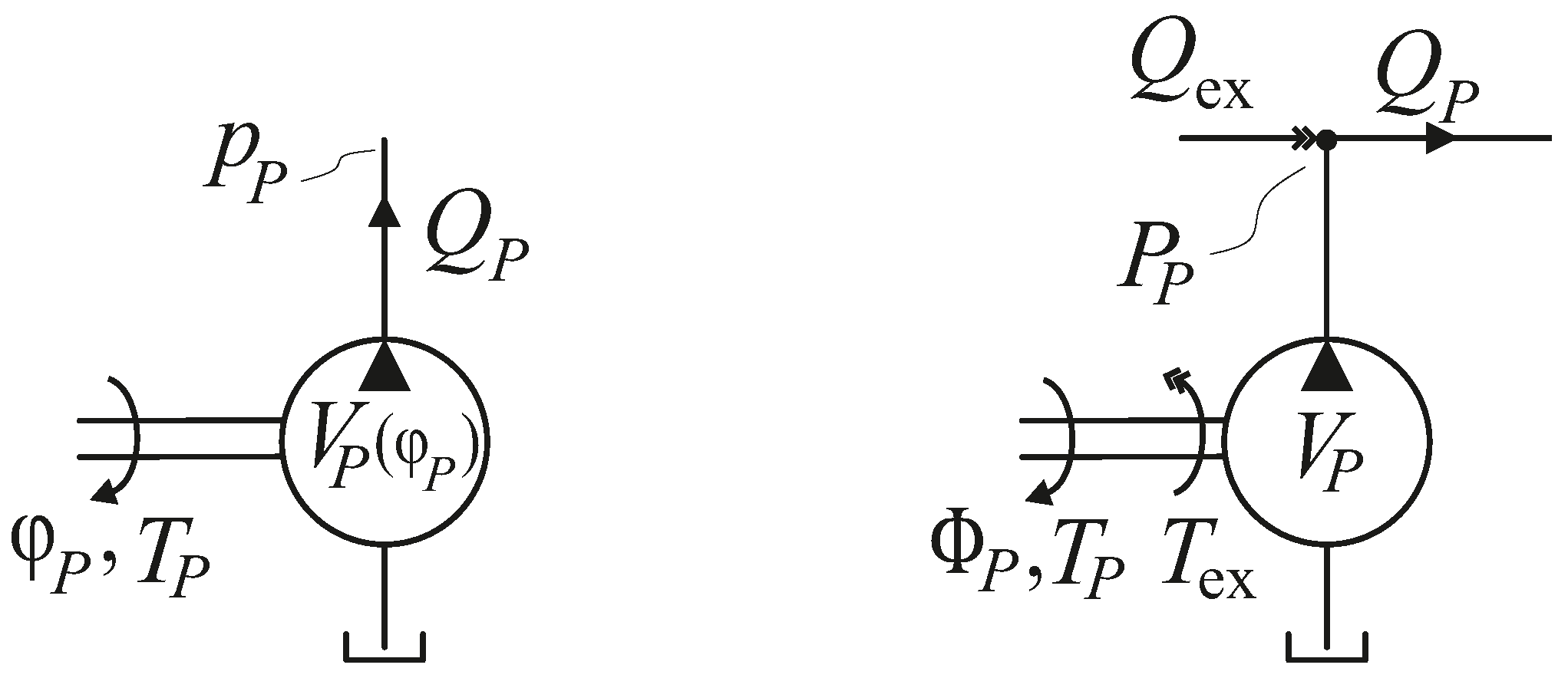
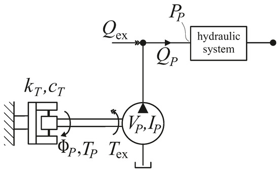
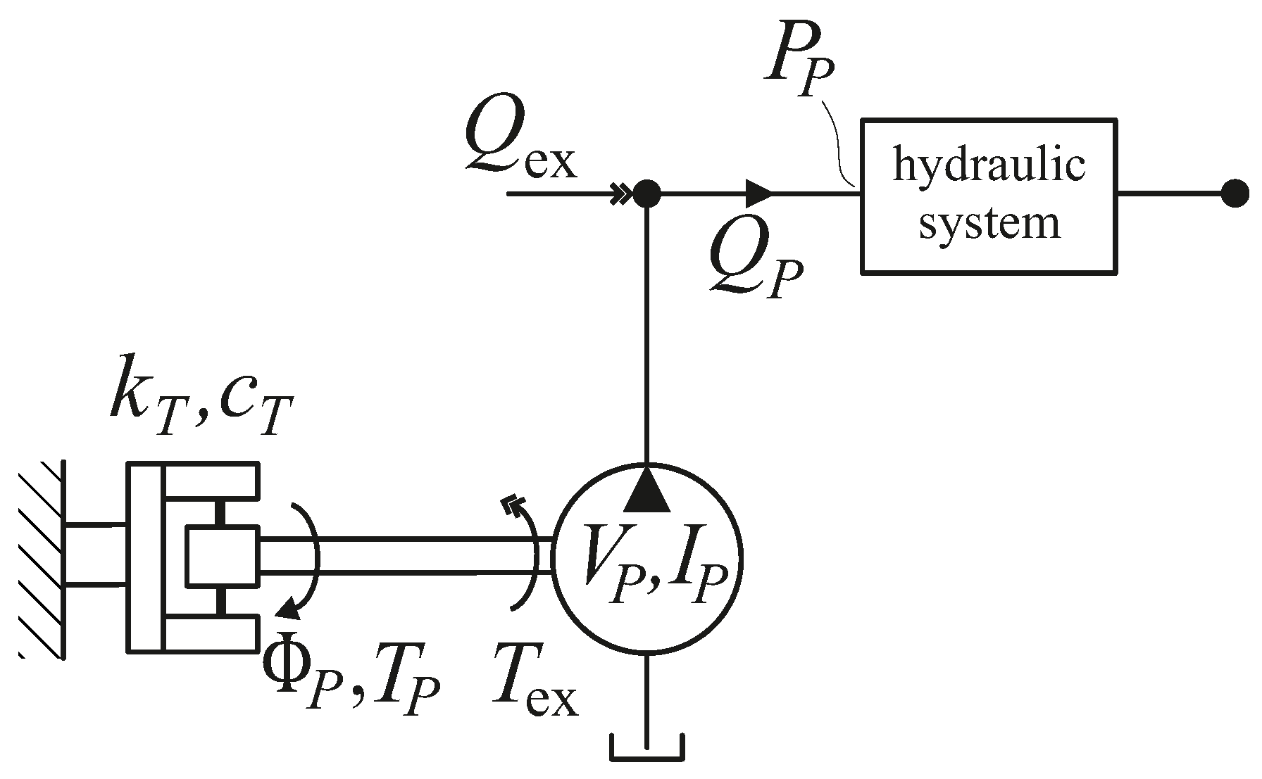
with denoting the pressure at the pump outlet. For frequency domain analysis, the nonlinear behaviour of the pump is linearised and represented by external excitations. The nonlinear time domain model of the pump corresponds to the left side of Figure 1, while the linearised frequency domain model, with external flow rate and torque excitation, is illustrated on the right side.
Figure 1.
Pump schematic for time domain (left) and frequency domain (right) model.
For linearisation, the pump is considered under stationary operating conditions, which allows the displacement to be expressed as a function of time. Only the first harmonic at the angular pulsation frequency is considered, which shall be justified in Section 6. The instantaneous displacement then becomes
with the mean displacement and the displacement amplitude . Accordingly, the state variables are composed of a mean component () and a first harmonic component (amplitudes: ). As functions of time, they are given by
The flow rate under stationary operating conditions becomes
The term proportional to arises from the product of the varying displacement and the varying angular velocity. As it represents a second-order contribution, it is neglected in the linearised frequency domain model, since the mean values of both quantities are significantly larger than their respective variations. This is obvious for the displacement of an external gear pump. According to [2], the non-uniformity grade of the flow rate of an external gear pump with 10 teeth is approximately 20%. Therefore, it can be concluded that is less than 10%. If the kinematic pulsation is fully compensated by the variation of angular velocity, the latter equals the variation in displacement. Under these conditions, the transformation of Equation (6) into the frequency domain yields
It consists of an angular velocity proportional flow rate component and a flow rate excitation component , which depends on the mean angular velocity of the pump (). The pulsation frequency is related to the mean angular velocity of the pump according to
where z denotes the number of teeth. Therefore, the external flow rate excitation can be expressed as
Using Equations (2), (3) and (5), the torque under stationary operating conditions becomes
The mean pressure is assumed to be significantly larger than the pressure variation. With the same simplifications as for Equation (7), the torque in the frequency domain can be expressed as
It consists of a term proportional to the pressure at the pump outlet and an excitation term , which depends on the mean pressure level .
2.2. Analytical Investigation of a Mechanical–Hydraulic System Coupled by an External Gear Pump
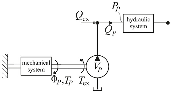
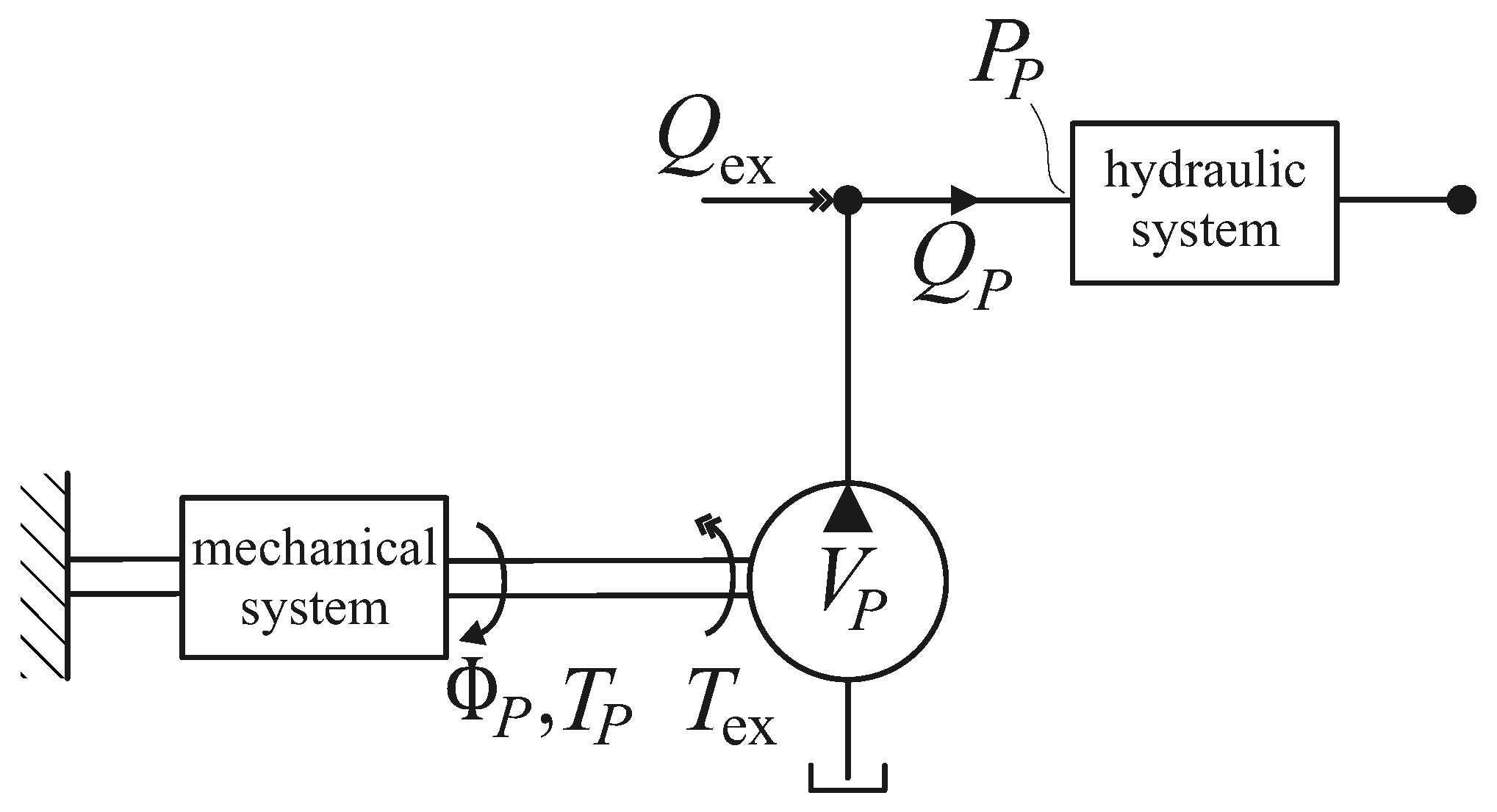
The external gear pump model is extended to include both a general mechanical system in the drivetrain and a general hydraulic system at the pump outlet, as shown in Figure 2. The mechanical and hydraulic subsystems are represented as linear four-pole networks relating torque and angular position on the mechanical side and pressure and flow rate on the hydraulic side.
Figure 2.
External gear pump with general mechanical and hydraulic systems modelled as linear four-pole networks.
In Figure 2, the mechanical system is shown schematically with a fixed angular boundary condition at its input. For any constant boundary condition at the input of the mechanical system, the angular position of the pump can be expressed in the frequency domain as
where denotes the linear transfer function of the mechanical system. Similarly, for the hydraulic system, under any constant boundary condition at the output, the pressure at the pump outlet can be expressed in the frequency domain as
where denotes the linear transfer function of the hydraulic system. Using Equations (7) and (11), the system can be expressed as
The pressure at the pump outlet results in
where is referred to as torque induced flow rate pulsation. If , the pressure pulsation at the pump outlet is cancelled irrespective of the hydraulic system. The necessary mechanical transfer function to cancel the pressure pulsation at the pump outlet is given by
Using Equations (9) and (11) results in
To achieve cancellation of the pressure pulsation, the mechanical system must provide a phase shift of . This cannot be achieved over the entire frequency range with a passive mechanical system, which becomes clear from the modal decomposition of the transfer function [19]. However, a spring–mass oscillator exhibits this phase shift at its undamped natural frequency.
2.3. Analytical Investigation of a Torsional Oscillator in the Drivetrain with a General Hydraulic System
Figure 3 shows a mechanical–hydraulic system with a specified mechanical subsystem, which includes a damped torsional oscillator in the drivetrain with the torsional stiffness , the damping coefficient , and the mass moment of inertia of the pump side . The torsional oscillator has a fixed boundary condition at the input. Due to the significantly higher inertia on the motor side, the two-mass drivetrain can be approximated as a restrained single-mass torsional oscillator. At the pump outlet, a general hydraulic system is considered, represented as a linear four-pole network.
Figure 3.
External gear pump with a damped single-mass torsional oscillator and a general hydraulic system modelled as a linear four-pole network.
The transfer function of the mechanical system is given by
with the undamped natural frequency
At the compensation frequency , the transfer function is given by
which fulfils the phase condition given by Equation (17). To cancel the pressure pulsation, the amplitude condition also needs to be fulfilled. Therefore, the damping coefficient of the torsional oscillator must be chosen as
The required damping value depends on constant pump parameters, the mean pressure at the pump outlet, and the compensation frequency. With the specified mechanical subsystem, pressure pulsations can be cancelled at the angular speed and the mean pressure level at the pump outlet, irrespective of the hydraulic system layout.
For , Equation (15) describes the compensation effect according to [12], which also applies in the present case. In particular, this effect was proven for the case that mechanical and hydraulic resonances coincide. Now, both compensation and cancellation come into play and pulsation reduction is particularly effective. The risk of parametric resonance in the drivetrain will be mitigated by the additional damping of the compensator.
3. Experimental Setup
3.1. Experimental Setup with Compensator Coupling and Damping Elements
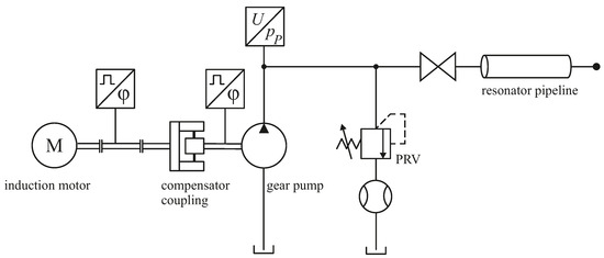
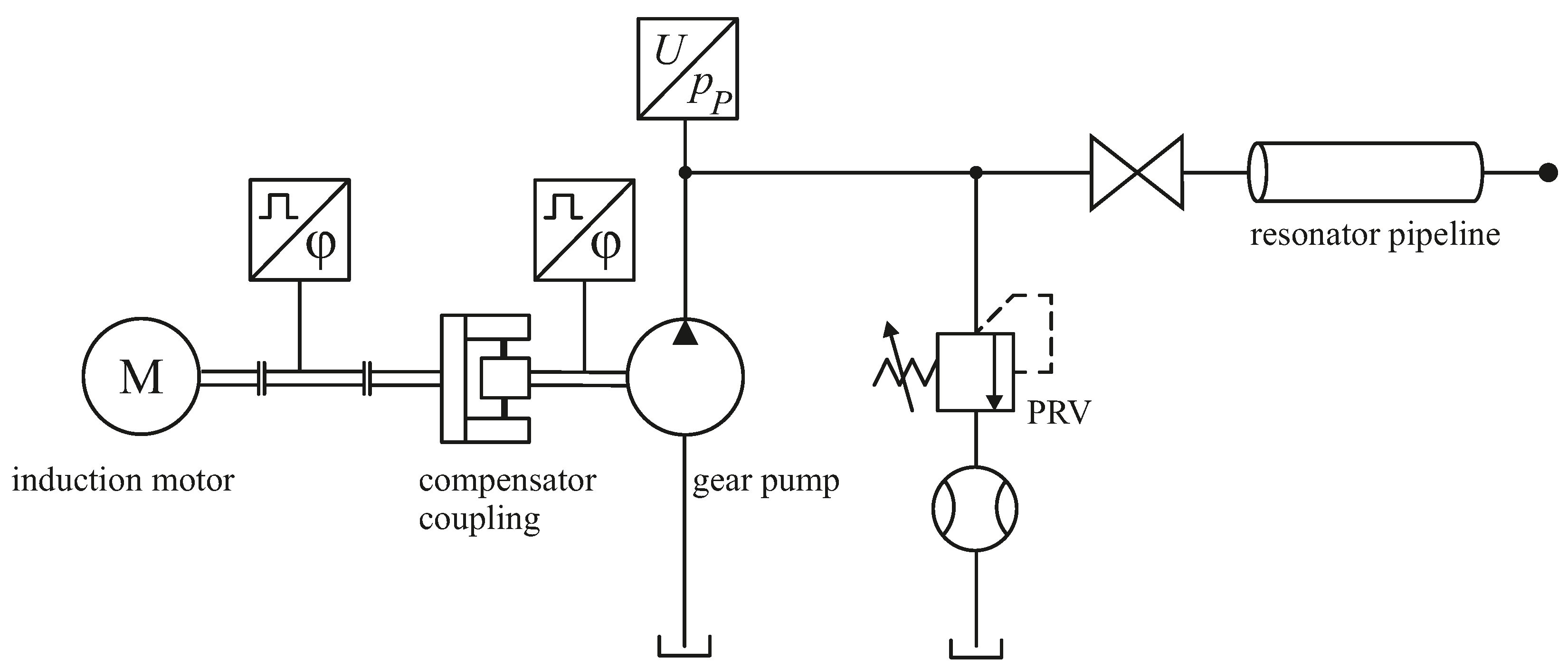
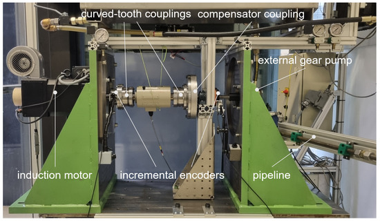
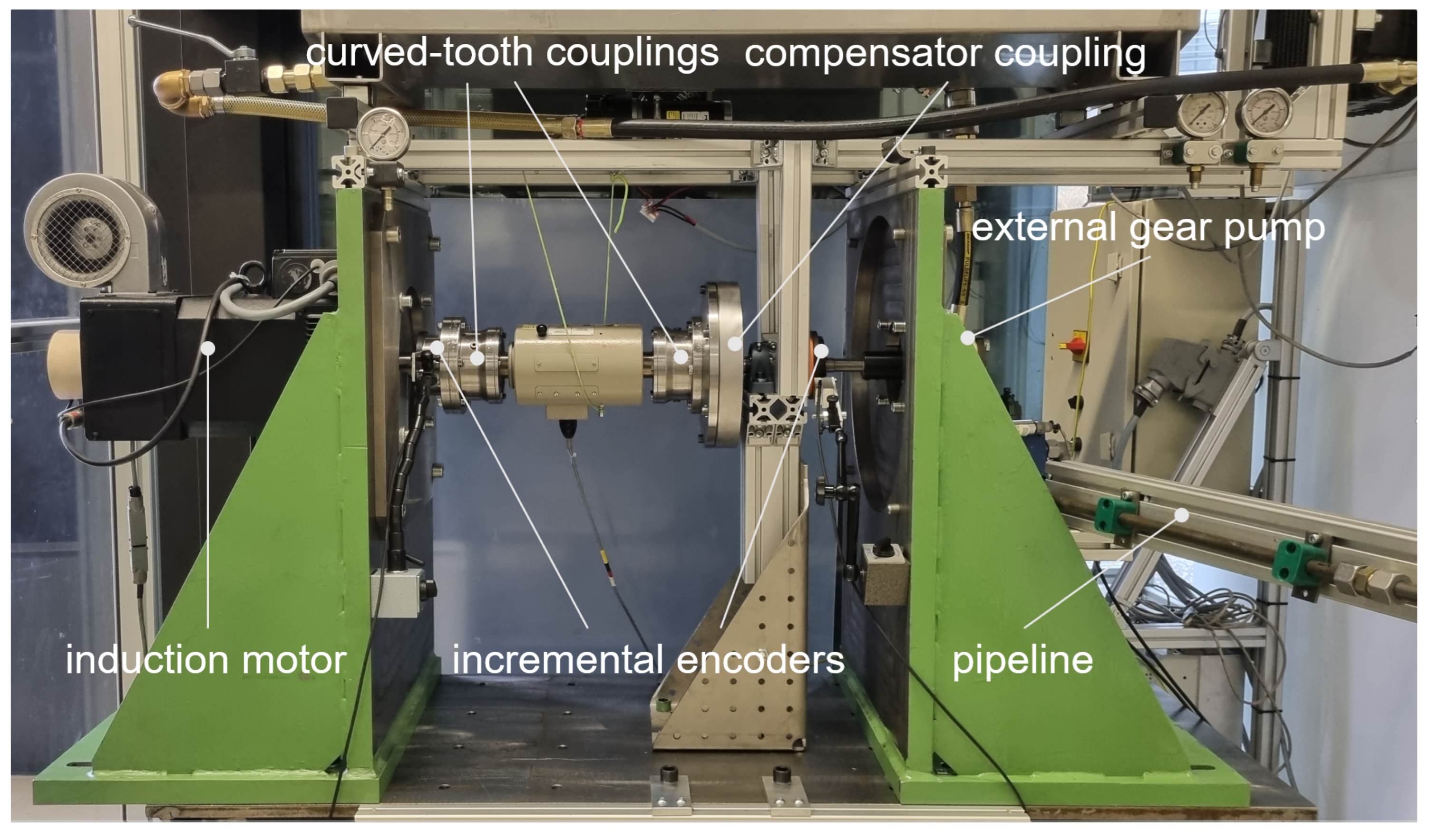
Figure 4 shows the overall layout of the experimental setup, including the mechanical drivetrain, the hydraulic system, and all sensors. The pump is driven by a speed-controlled induction motor. The drivetrain comprises a shaft connected to the motor and to the compensator coupling by curved-tooth couplings, the compensator coupling, and an external gear pump. The external gear pump is connected to the compensator coupling via an adapter shaft and is supported by an auxiliary bearing, as shown in Figure 5. The angular positions of the motor and the pump are recorded using magnetic incremental encoders (LM10, RLS, Ljubljana, Slovenia). The magnetic ring comprises 160 poles, while the readhead provides an incremental output with an interpolation factor of 1024 counts per pole, resulting in a total resolution of 163,840 counts per revolution.
Figure 4.
Overall layout of the experimental setup including drivetrain and hydraulic system.
Figure 5.
Experimental test rig with rotary mechanical pulsation compensator.
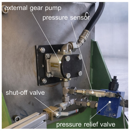
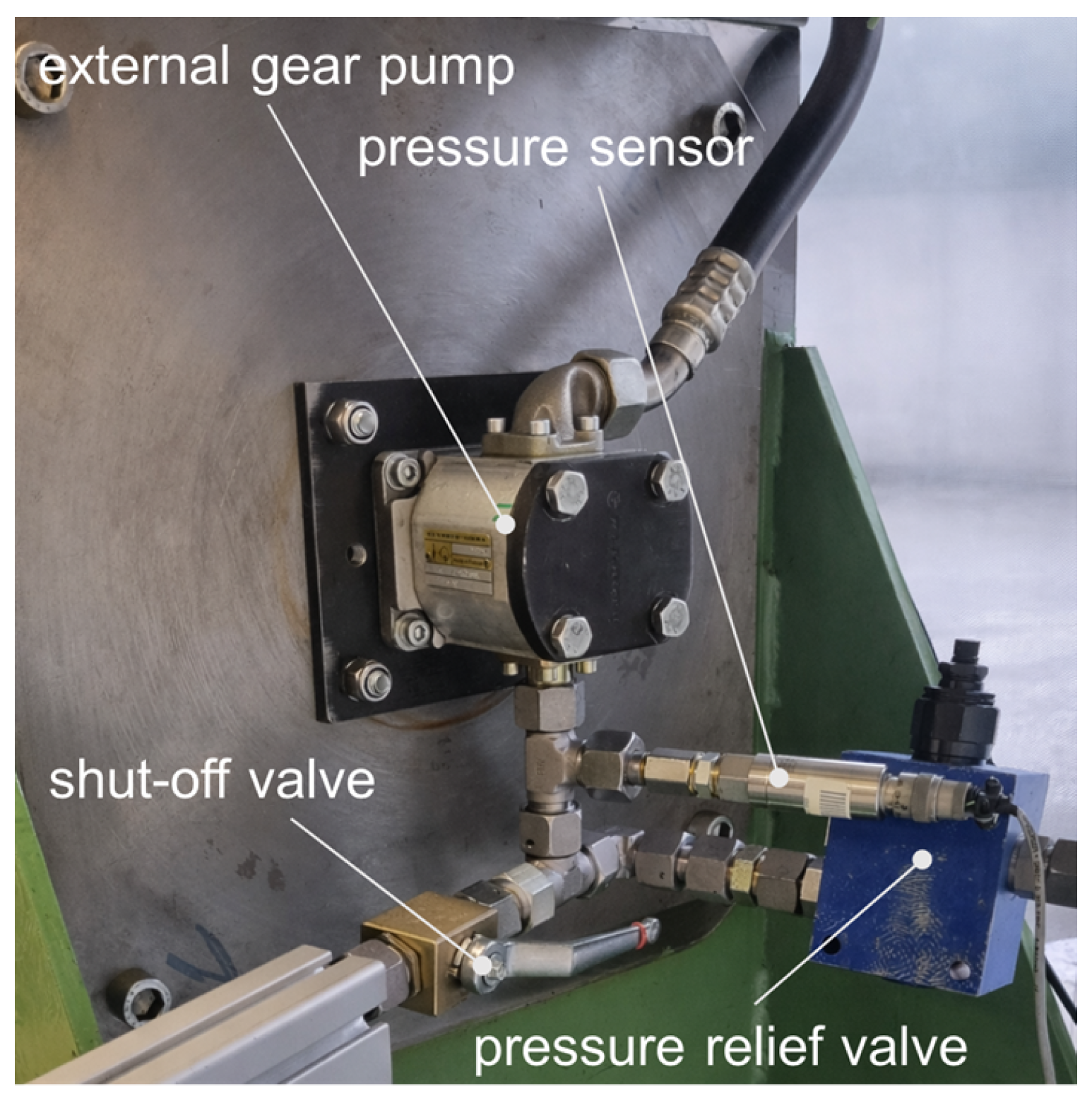
The pump and the hydraulic system, including a pressure relief valve and a resonator pipeline at the pump outlet, are shown in Figure 6. The pipeline can be disconnected via a shut-off valve in order to investigate two different hydraulic configurations. The first is a closed pipeline, which exhibits a significant hydraulic resonance, and the second is a configuration that includes only the pressure relief valve. A piezoresistive pressure sensor (PDCR 4060, Druck, Leicester, UK) with a measurement range of 0–200 bar and a specified accuracy of full scale is installed downstream of the pump outlet.
Figure 6.
Hydraulic components of the experimental setup.
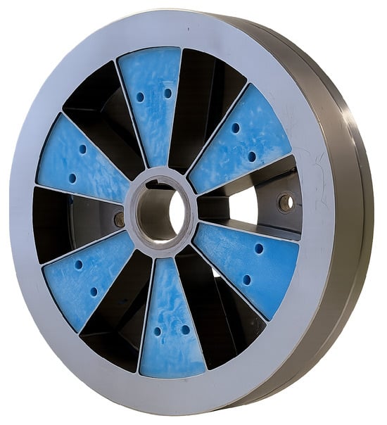
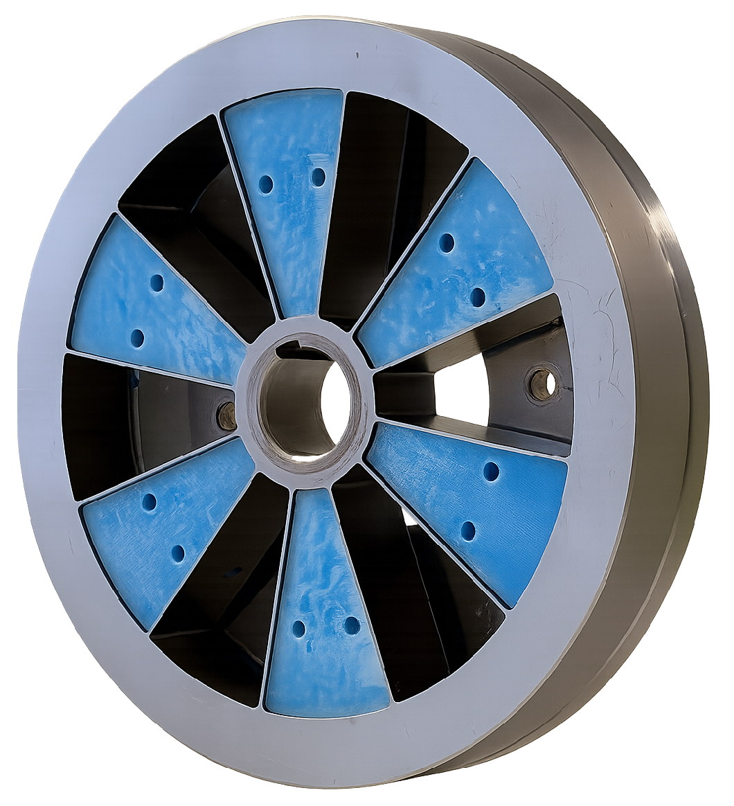
As described in [15], the mass moment of inertia on the pump side should be as small as possible to obtain broadband pulsation compensation. The design objective was therefore to obtain the required torsional stiffness while keeping the mass moment of inertia on the pump side low. To meet these requirements, the compensator is designed as a spoke wheel, as illustrated in Figure 7.
Figure 7.
Compensator coupling with damping elements.
The inner ring is connected to the pump side, whereas the outer ring is connected to the motor side via a flange. The inner and outer rings of the spoke wheel are connected by twelve radial beams. Relative rotation between the inner and outer rings causes elongation of the radial beams, leading to tension stresses. As a result, the torsional stiffness of the coupling increases with increasing torque. This nonlinear behaviour shifts the compensation frequency depending on the system pressure.
To adjust the damping of the compensator coupling according to Equation (21), 3D-printed damping elements are used. Six of these elements are inserted into the compensator shown in Figure 7. In total, up to twelve elements can be installed, with attention paid to maintaining mass balance. For the 3D-printed damper elements made of thermoplastic polyurethane (TPU), infill structures such as gyroid or honeycomb are suitable [20]. To minimise the influence on the natural frequency of the compensator, both the stiffness of the damper elements and their mass moment of inertia should be kept low. To achieve the required damping values, a 3D-printed damper concept with a two-phase infill is applied as described in [21]. Accordingly, a gyroid structure with a 15% infill was selected and filled with soft silicone (Shore hardness 20). This approach enables a combination of material, structural, and viscous damping mechanisms. The gyroid structure ensures full interconnectivity of all internal voids, allowing silicone injection through a single inlet. The damping elements are prototypes designed to achieve the required damping effect in the laboratory. The focus is on simple manufacturing, low stiffness, and low mass moment of inertia. Thermal behaviour, long-term use, and hysteresis effects have not been investigated.
3.2. Measurement Setup, Data Acquisition, and Signal Analysis
As the individual excitations are difficult to measure, the system’s transfer functions are not determined directly. Instead, the pressure at the pump outlet is considered.
To analyse the system behaviour based on the pressure pulsation in the frequency domain, the pressure at the pump outlet and the angular position of the pump shaft are required. While the displacement amplitude is not exactly known, the displacement phase depends on the angular position of the pump shaft, allowing the relative phase of the pressure pulsation to be determined. For data acquisition, an NI PCIe-6323 data acquisition card (National Instruments, Austin, TX, USA) in combination with MATLAB/Simulink Desktop Real-Time R2024b is used. Both signals are sampled at 10 kHz. Since the investigated frequency range is limited to below 1 kHz, and no relevant high-frequency signal components are expected to affect the evaluated spectra, no additional analogue anti-aliasing filters are included.
In the experiments, a stepwise speed profile is applied. The motor performs ten revolutions at each speed step, which allows for a series of measurements within an acceptable time. Starting at 500 revolutions per minute, as specified as the minimum speed in the data sheet [22], the rotational speed is increased by four revolutions per minute at each step. The experiment ends at a rotational speed of 2300 revolutions per minute, which is the limit of the induction motor. In total, 451 speed steps with quasi-stationary operating conditions are evaluated. The rectangular evaluation window is triggered by the angular position of the pump shaft.
Since the excitation frequency equals the pulsation frequency and the amplitude of the first displacement harmonic is the same for all frequencies, the Fourier coefficients of the first pressure harmonic are determined. Higher-order harmonics are not considered. The signal processing yields the amplitude of the pressure response and its phase relative to the pump displacement for each speed step.
Out of ten revolutions at each step, the first four revolutions are discarded to ensure that the system is as close as possible to steady state conditions. The last revolution is omitted to ensure that only complete revolutions are considered. Consequently, five complete revolutions are used for the evaluation.
The Fourier coefficients of the first harmonic are calculated as
where N denotes the total number of samples used for the evaluation, the number of samples per pulse, and the discrete signal. The coefficients and correspond to the cosine and sine components of the first harmonic. The amplitude of the first harmonic is given by
and the phase is determined as
4. Modelling and Parameter Identification
4.1. Frequency Domain Model of the Experimental Setup
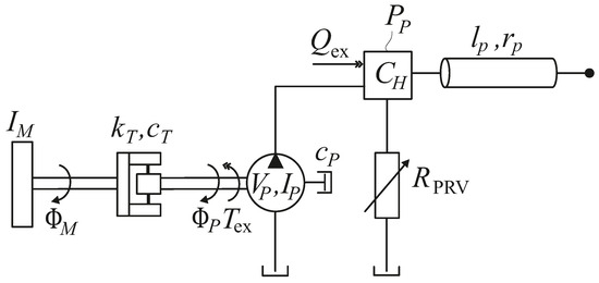
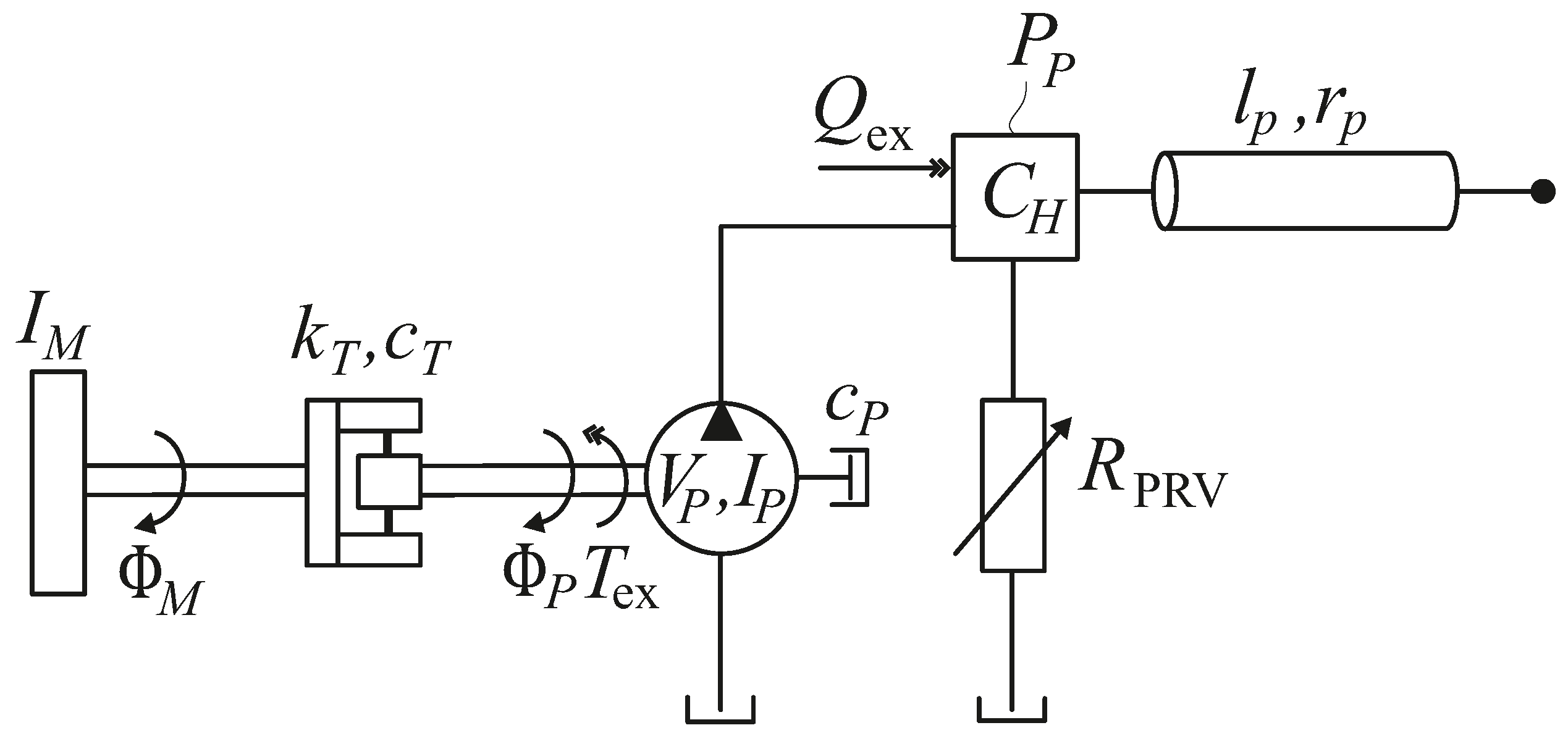
To calculate the effect of the compensator coupling, the experimental setup is modelled in the frequency domain. Figure 8 shows a schematic representation of the system. The mechanical drivetrain is modelled as a two-mass torsional oscillator with the mass moments of inertia on the motor side and on the pump side. The compensator coupling is represented by the torsional stiffness and the damping coefficient . In addition, the mechanical losses of the pump are taken into account by an equivalent damping coefficient . still denotes the mean displacement of the pump. The excitations and are given in Equations (9) and (11), respectively.
Figure 8.
Mechanical–hydraulic system with the rotary mechanical pulsation compensator.
As described in [23], the outlet of a pump exhibits capacitive behaviour. Therefore, the hydraulic capacitance is considered at the pump outlet. The capacitance also includes the effective hydraulic capacitance of the connection volumes associated with the pressure relief valve and the resonator pipeline. The pressure relief valve, modelled as a frequency-dependent hydraulic resistance , and the resonator pipeline with inner radius and length are connected to the outlet capacitance . The coupled hydraulic–mechanical system can be expressed in the frequency domain in the form of an equation of motion as
with the mass matrix , the damping matrix , the stiffness matrix , the state vector , and the excitation vector . The state variables of the model are the angular position of the motor , the angular position of the pump , and the pressure at the pump outlet . Equation (25) can be written explicitly as
The function
with
and
represents the transfer function of a closed-end pipeline according to the dynamic laminar pipeline model proposed in [24]. E, , and denote bulk modulus, density and kinematic viscosity of the fluid, respectively. and are Bessel functions of first kind. For the calculations without resonator pipeline, is set to zero.
At low frequencies, the pressure relief valve can be modelled as a variable orifice
where denotes the flow rate through the pressure relief valve, is an opening coefficient that depends on the pressure at the pump outlet, and the pressure at the tank. Since , the tank pressure is approximated by . The cut-off frequency of the pressure relief valve is approximately 100 Hz, which is significantly lower than the excitation frequencies of interest (above 200 Hz). For these higher frequencies, the pressure relief valve can be modelled as an orifice with a constant opening coefficient
which depends on the mean pressure level and the mean flow rate. The mean flow rate is given by
The flow rate through the pressure relief valve then becomes
Linearisation around the operating point yields
In the frequency domain, the flow rate through the pressure relief valve is given by
Using Equations (8), (32) and (35), the frequency dependent hydraulic resistance results as
It is assumed that the entire flow rate is discharged through the pressure relief valve. The volumetric efficiency of the pump, determined for the relevant operating points, is approximately . Therefore, leakage losses are not modelled separately.
The pressure at the pump outlet, which is the relevant output variable of the overall system, follows from the superposition principle as
in which the transfer function between pressure pulsation and torque excitation and the transfer function between pressure pulsation and flow rate excitation can be determined from Equation (26).
4.2. Parameter Identification
In Table 1, the relevant system parameters are listed. Several parameters depend on the operating conditions and are therefore specified separately for the first experiment at an operating pressure of 170 bar and the second experiment at an operating pressure of 100 bar. Some parameters are not exactly known and identified step by step from dedicated measurements as detailed below. All measurements are performed at an oil temperature of approximately 50 °C to ensure consistent operating conditions and to minimise the influence of temperature-dependent fluid properties. To identify the hydraulic system, calculations and measurements without the compensator are used. The corresponding model with a rigid drivetrain is given by
where denotes the mass moment of inertia of the entire drivetrain. The natural frequency of the hydraulic system depends on the hydraulic capacitance at the pump outlet as well as on the pipeline and fluid parameters. By comparing the natural frequencies obtained from calculations and measurements, the hydraulic capacitance at the pump outlet can be identified. The displacement amplitude is determined by matching calculated and measured amplitudes.
Table 1.
Model parameters for Experiment 1 (170 bar) and Experiment 2 (100 bar).
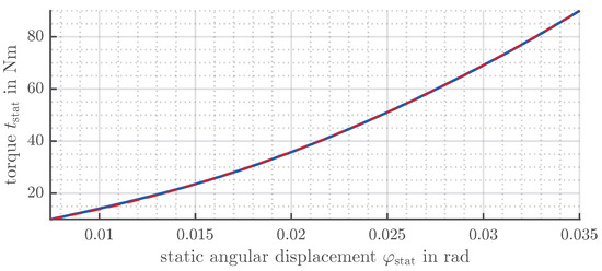
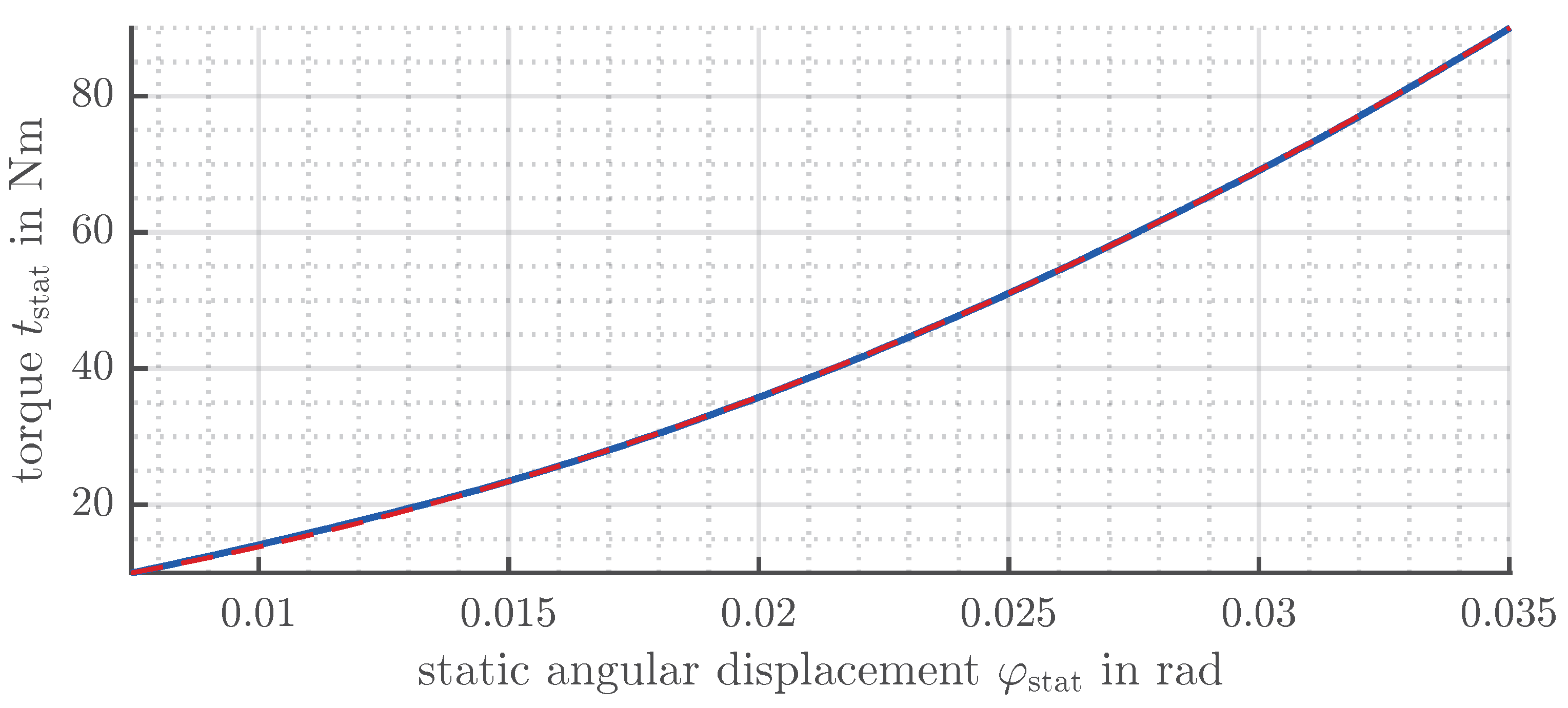
To determine the stiffness of the compensator at the operating point, a static measurement with six damping elements is carried out. For this purpose, the inner ring of the compensator is fixed while a torque is applied to the outer ring. The resulting angular displacement is measured using the same incremental encoders as described in Section 3.1. The applied torque is measured using a torque measurement shaft (T22, HBK, Darmstadt, Germany) with a nominal measuring range of 200 Nm and an accuracy class of 0.5. Figure 9 shows the relationship between the angular displacement and the applied torque. To determine the local torsional stiffness, a quadratic function (red dashed line) is fitted to the measured data (blue line). The local stiffness is then obtained as the derivative of the fitted function,
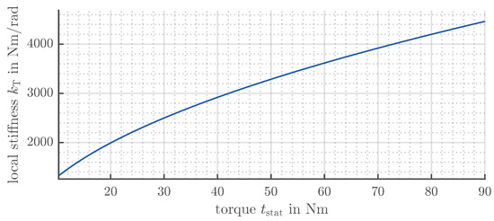
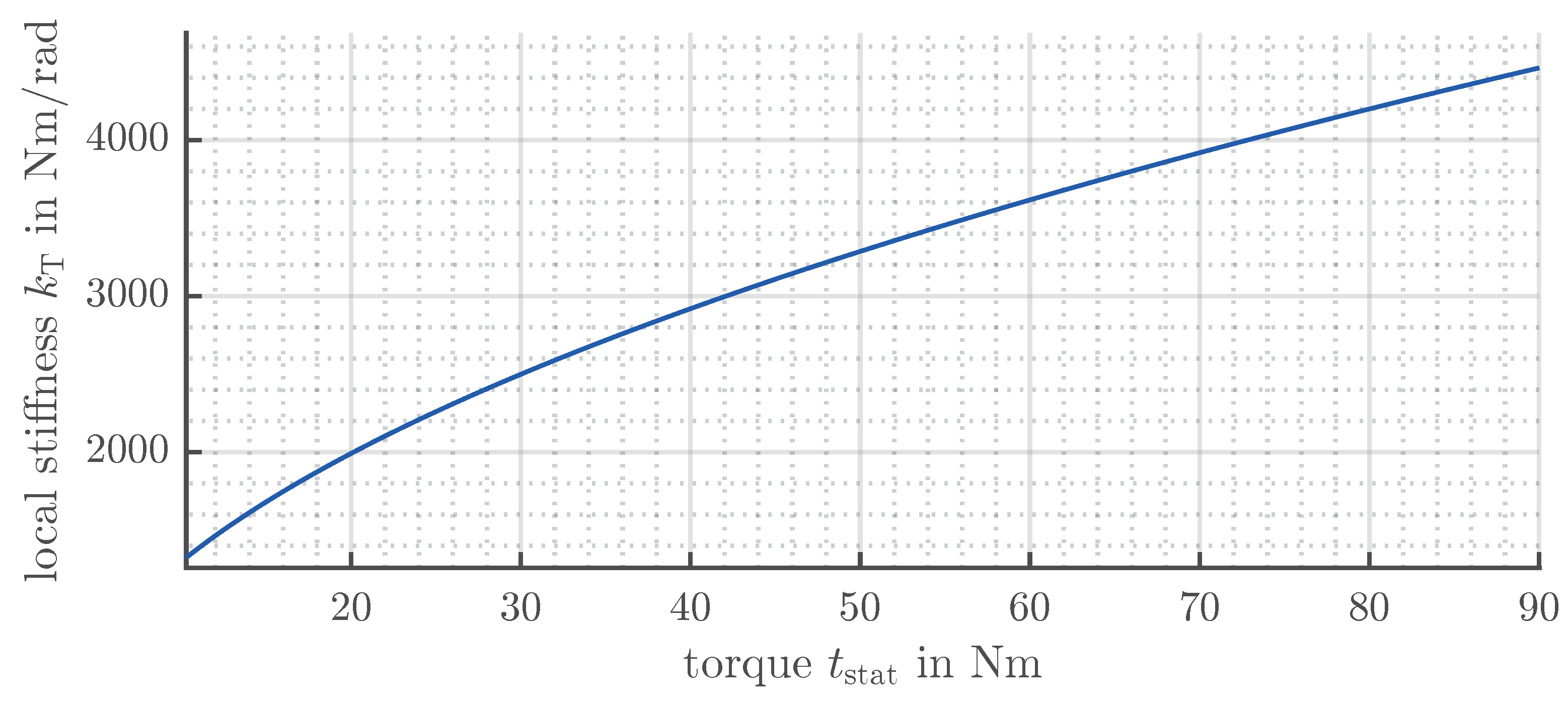
and shown in Figure 10. According to the torque-pressure characteristic given in the data sheet of the external gear pump [22], the transmitted torque is approximately 58 Nm at a mean pressure of 170 bar (Experiment 1) and approximately 33 Nm at a mean pressure of 100 bar (Experiment 2). This results in torsional stiffness of the compensator coupling at the operating point of 3560 Nm/rad and 2630 Nm/rad for Experiments 1 and 2, respectively.
Figure 9.
Static torque–angle characteristic of the compensator with six damping elements. Blue: measured data; red dashed: fitted quadratic function.
Figure 10.
Local torsional stiffness of the compensator.
The natural frequency of the mechanical system depends on the stiffness of the compensator coupling and on the mass moments of inertia on the pump and motor sides. The mass moment of inertia on the pump side is only known approximately because the contributions of the radial beams and the damping elements have not been quantified explicitly. The mass moment of inertia on the motor side is primarily determined by the motor, the shaft, an intermediate flange, and the outer ring of the compensator coupling, while the additional contributions of the radial beams and the damping elements are negligible. The undamped natural frequency of the mechanical system corresponds to the compensation frequency observed in the measurements presented in Section 6. For Experiment 1 with six damping elements, the natural frequency is 323 Hz with resonator pipeline and 320 Hz without resonator pipeline. The observed deviation can be attributed to slight differences in the mean pressure level and oil temperature. For Experiment 2 with six damping elements, the natural frequency is 273 Hz with resonator pipeline and 274 Hz without resonator pipeline. With
the mass moment of inertia on the pump side can be determined. The calculated values range from to , corresponding to a deviation of approximately 5%. For the model, the mean value of is used. Furthermore, the influence of the damping elements on the stiffness of the compensator, as well as on the mass moments of inertia of the pump and motor sides, is neglected in the model.
The mechanical losses of the pump can be determined from the torque-pressure characteristic given in the data sheet [22]. These losses are represented by the equivalent damping coefficient , for which
applies. Using Equation (8), the frequency-dependent damping coefficient can be expressed as
The damping behaviour of the compensator with damping elements is nonlinear and depends on the operating conditions. For each calculation, the damping coefficient is determined from the optimum configuration of the measurement with resonator pipeline using Equation (21). Assuming identical damping elements and a linear contribution with the number of elements, the damping coefficient per element can be determined. In the model, this result is used for all damping configurations, and in both configurations of the hydraulic system.
5. Frequency Domain View on Pulsation Cancellation
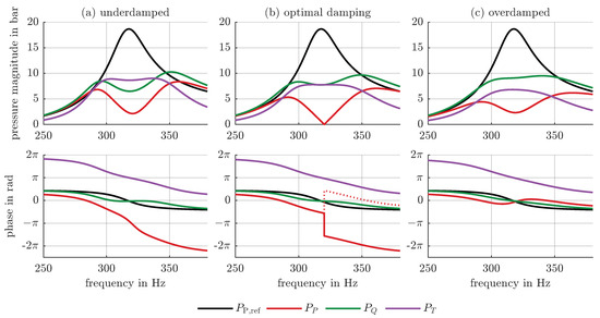
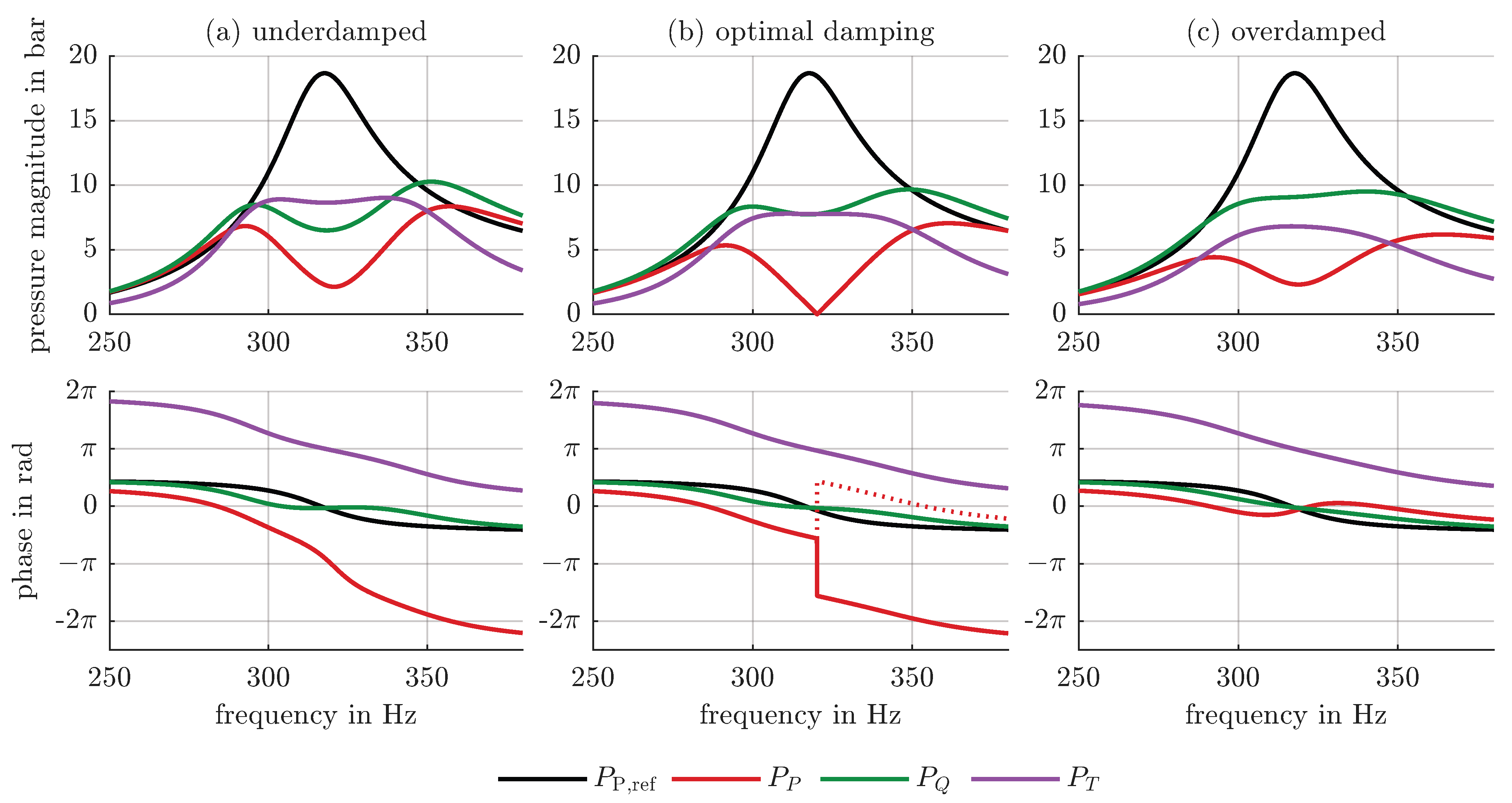
The pressure pulsation cancellation effect is achieved by tuning two excitations, which appear in Equation (15) as external flow rate excitation and torque excitation . Figure 11 shows the calculated frequency domain results for a system with a resonator pipeline. The pressure pulsations caused by the two excitations are shown separately, along with the total pressure pulsation in the system. For reference, the pressure pulsation without the compensator is shown in black. The natural frequency of the hydraulic system occurs at 320 Hz and corresponds to the compensation frequency. According to Equation (37), the pressure pulsation resulting from the external flow rate excitation is given by
whereas the pressure pulsation caused by the torque excitation is expressed as
Figure 11b corresponds to the optimal damping value. At the compensation frequency of 320 Hz, the magnitudes of the pressure pulsations due to flow rate excitation (green) and torque excitation (purple) are equal. The phase shift between the signals is , which results in the complete cancellation of the total pressure pulsation (red). The underdamped case is shown in Figure 11a. At the compensation frequency, the pressure pulsation caused by torque excitation is higher than the pressure pulsation caused by flow rate excitation. In the overdamped case, shown in Figure 11c, the pressure pulsation due to flow rate excitation dominates. Complete cancellation cannot be achieved in either an underdamped or overdamped case. However, significant reductions in pressure pulsation are obtained compared to the system without compensator. Moreover, no pronounced side resonances are observed due to the damping in the system.
Figure 11.
Frequency domain results for the hydraulic system with a closed pipeline for different damping values: (a) underdamped (), (b) optimal damping (), (c) overdamped (). Black denotes the reference pulsation without compensator, red the pulsation with compensator, green the pulsation due to flow rate excitation, and purple the pulsation due to torque excitation.
The pressure pulsations and cannot be measured separately. To distinguish between underdamped and overdamped cases, the phase of the total pressure pulsation is evaluated. The pressure pulsation at the compensation frequency can be written as
where denotes the phase of the pressure pulsation caused by the flow rate excitation, and denotes the phase of the pressure pulsation caused by the torque excitation. Equations (9), (11), (15) and (20) show that, at the compensation frequency, the phase difference between the flow rate excitation and the torque induced flow rate pulsation equals , such that . This yields
If complete cancellation occurs, such that , the amplitude of the total pressure pulsation becomes zero and the phase is undefined. In the underdamped case, , the phase of the total pressure pulsation is
as shown in Figure 11a. In the overdamped case, , illustrated in Figure 11c, the phase of the total pressure pulsation is
In Figure 11b, the phase response for nearly optimal damping is shown. The solid red line represents the phase response for slightly insufficient damping, where the phase exhibits a jump of at the compensation frequency. For damping that is slightly too high (dotted red line), the phase jump amounts to .
6. Experimental Proof and Model Validation
The following section presents measurement results obtained at two different mean pressure levels, both with and without a resonator pipeline. For the higher mean pressure level, calculated results are also included.
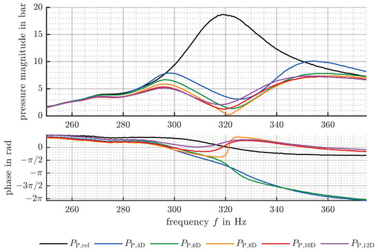
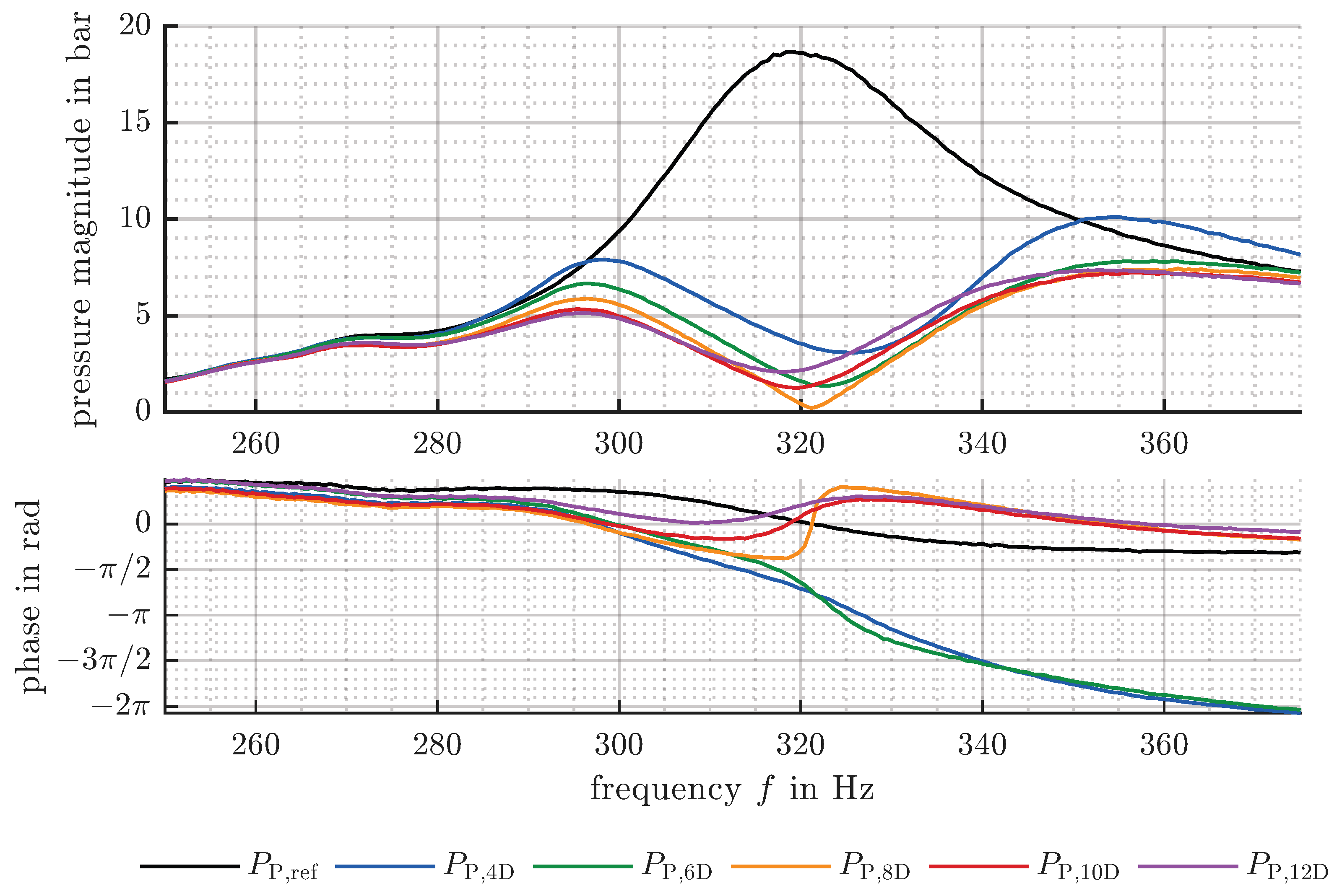
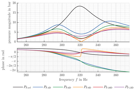
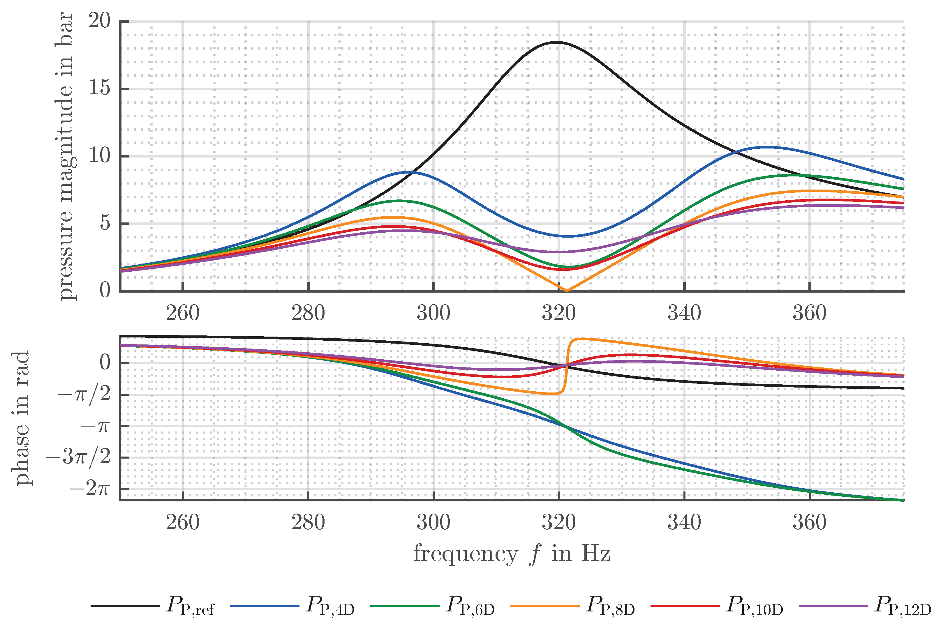
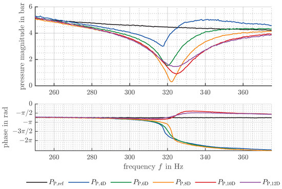
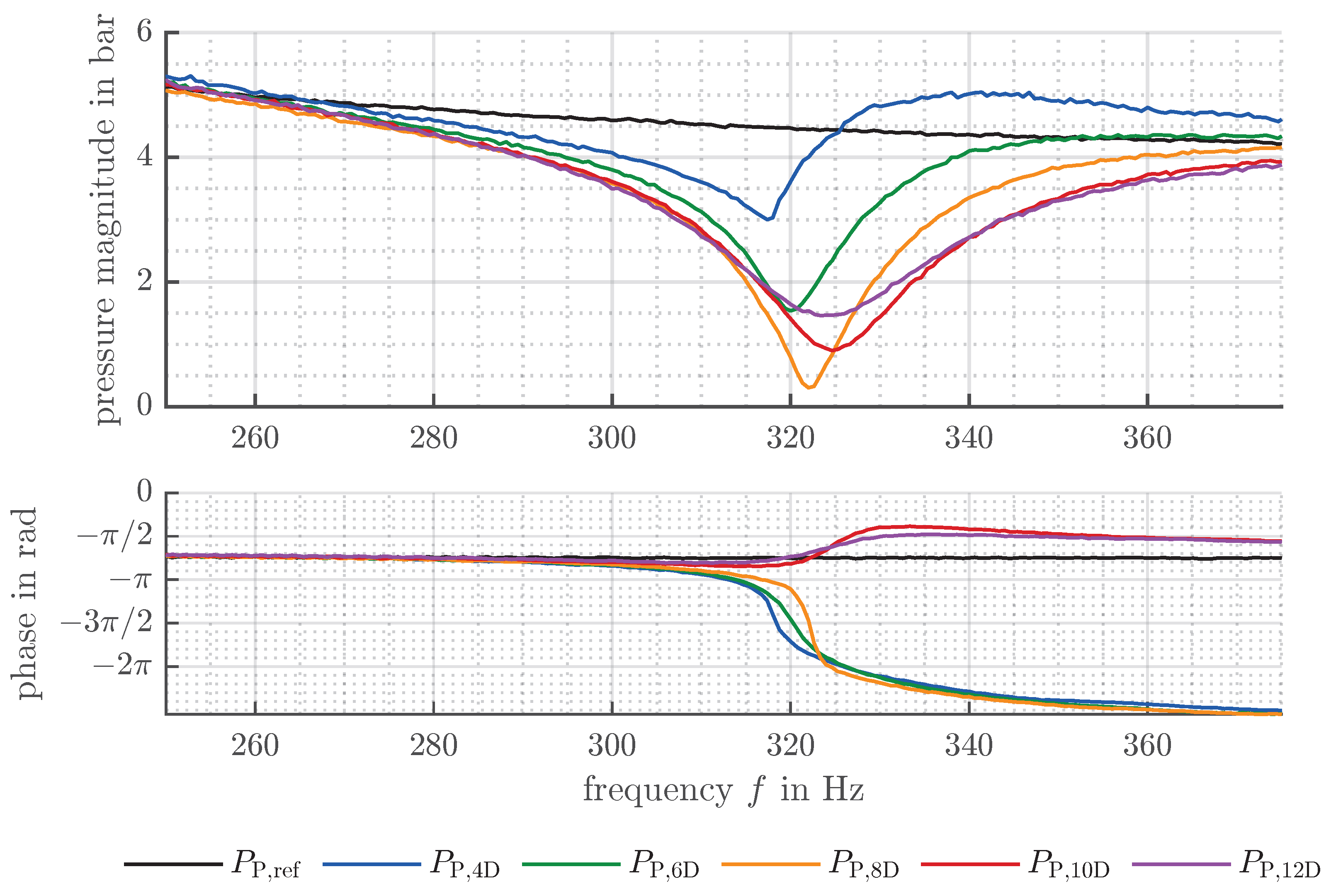
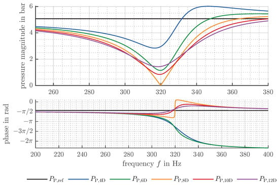
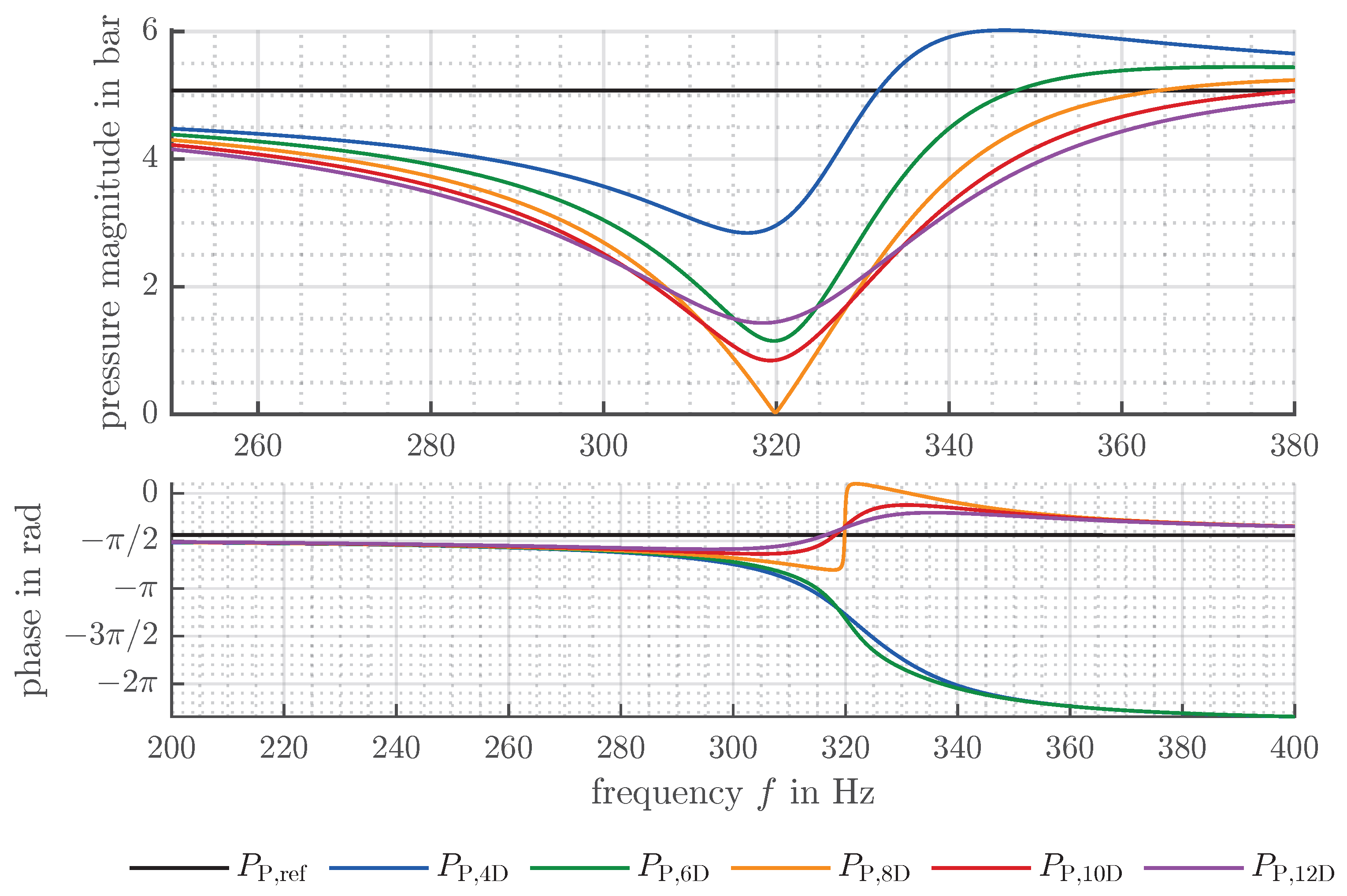
In the first experiment, a pipeline length of 1.54 m and a mean pressure level of 170 bar are considered. Figure 12 shows the measurement results for five different damping values together with a reference measurement without compensator (black). The corresponding theoretical results are presented in Figure 13. The configuration with eight damping elements (shown in orange) achieves pressure pulsation cancellation at the compensation frequency. In both theory and measurement, the magnitude of the pressure pulsation is reduced from 18.5 bar to 0.3 bar, which corresponds to a reduction rate of 98%. The pressure pulsation is significantly reduced within a frequency range from 290 Hz to 370 Hz, corresponding to a rotational speed range from 1740 to 2220 rev/min. Based on the phase response, it can be concluded that the damping value is marginally higher than the optimal value. Among all investigated configurations, the variant with four damping elements (blue) shows the poorest performance, exhibiting higher pressure pulsations over the entire investigated frequency range compared to the other configurations. Variants with lower damping will perform worse and are therefore not considered further. In contrast, damping values above the optimum tend to reduce the pressure pulsation at the side resonances. The configuration with twelve damping elements (purple) still shows a pronounced reduction at the compensation frequency despite the comparatively high damping value. All the investigated configurations yield satisfactory results, demonstrating the robustness of the damping adjustment.
Figure 12.
Measurement results for a closed pipeline with a length of 1.54 m and a mean pressure level of 170 bar. The upper plot shows the pressure magnitude and the lower plot shows the phase response. Black: system without compensator; blue: 4 damping elements; green: 6 damping elements; orange: 8 damping elements; red: 10 damping elements; purple: 12 damping elements.
Figure 13.
Calculated results for a closed pipeline with a length of 1.54 m and a mean pressure level of 170 bar. The upper plot shows the pressure magnitude and the lower plot shows the phase response. Black: system without compensator; blue: 4 damping elements; green: 6 damping elements; orange: 8 damping elements; red: 10 damping elements; purple: 12 damping elements.
Using Equation (21), the optimal damping for a mean pressure level of 170 bar and a compensation frequency of results in
Based on this value, the damping coefficient of the compensator is obtained as
with the damping coefficient of the pump from Equation (42). Assuming identical damping elements and neglecting the damping of the compensator without damping elements, the damping coefficient per element at this operating point becomes
With the identified parameters, very good agreement between measured and theoretical pressure pulsation is obtained for five different values of damping (see Figure 12 and Figure 13). Table 2 summarises the root mean square error (RMSE) and the normalized root mean square error (NRMSE) of the pressure magnitude for the reference measurement without compensator and for the experiments with different numbers of damping elements. The error metrics are calculated over the investigated frequency range from 250 Hz to 380 Hz. The NRMSE is normalised with respect to the maximum measured pressure pulsation amplitude. Despite neglecting the influence of the different numbers of damping elements on the stiffness and pump sided mass moment of inertia, RMSE and NRMSE values confirm that the proposed linear theoretical model reflects the dynamic behaviour of the system over the investigated frequency range.
Table 2.
Quantitative comparison between calculation and measurement for the experiment with resonator pipeline at 170 bar.
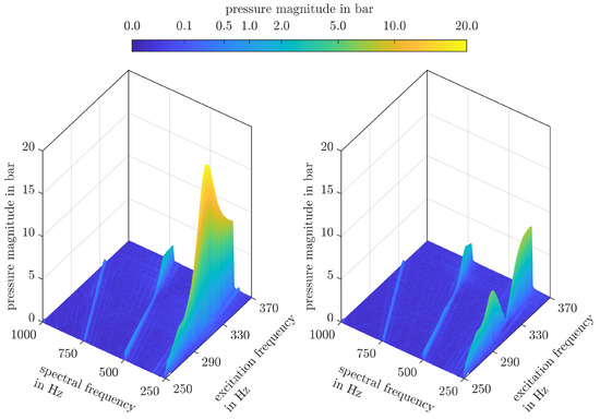
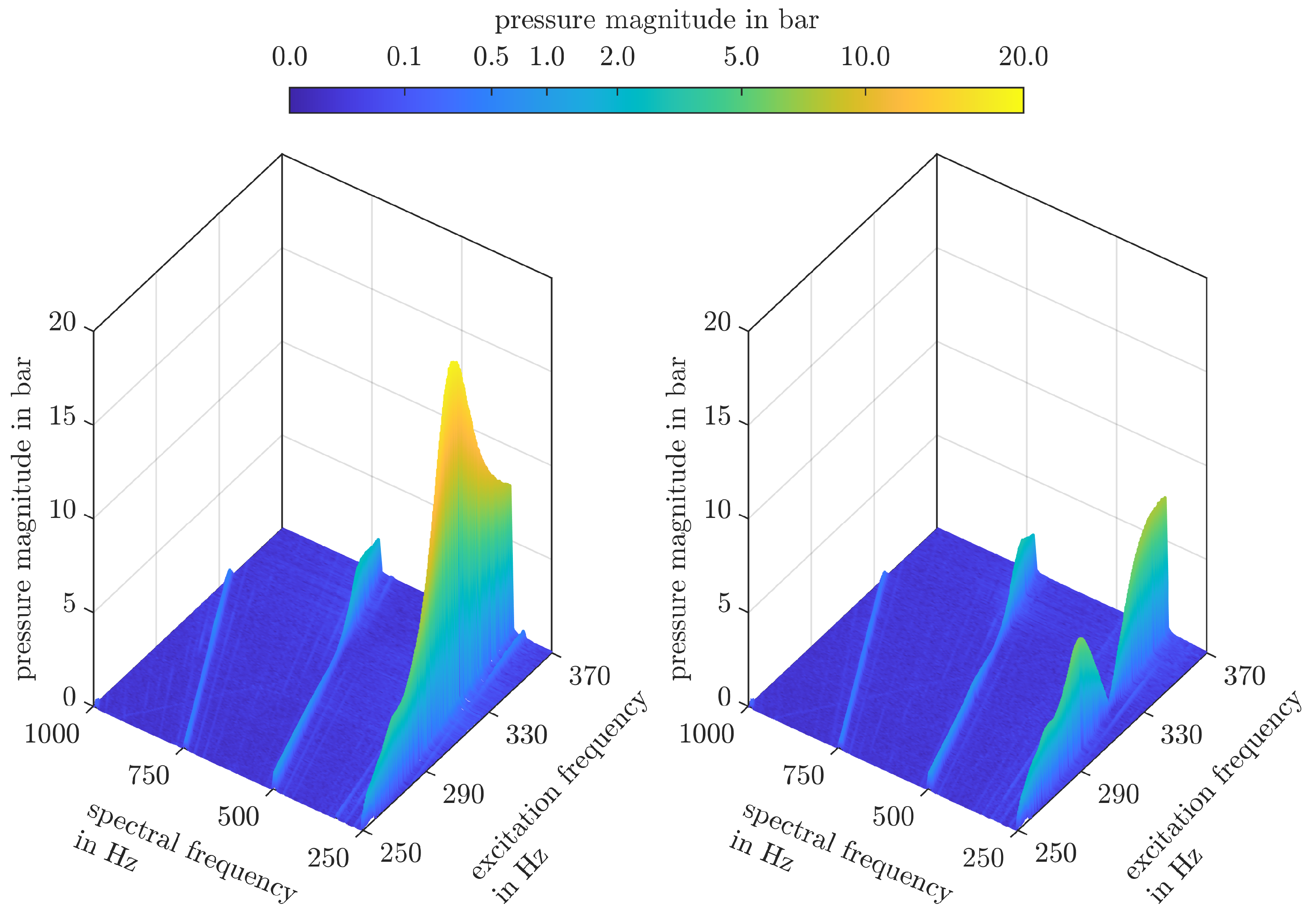
To assess the role of higher pulsation harmonics, Fast Fourier Transforms of the pressure signal are shown in Figure 14. For each speed step, the Fast Fourier Transform is applied using the rectangular window described in Section 3. Since the segment length varies with rotational speed, the individual spectra have different frequency resolutions and are interpolated to a common spectral frequency axis for the graphical representation. Figure 14 shows the spectra without compensator on the left and those with compensator on the right. It can be seen that both responses are dominated by the fundamental pulsation frequency.
Figure 14.
Pressure spectra over the excitation frequency without compensator (left) and with compensator using eight damping elements (right).
The measurement results for the experiment at a mean pressure level of 170 bar without a pipeline are shown in Figure 15, and the corresponding theoretical results are presented in Figure 16. Even in the absence of pronounced hydraulic resonance, the compensator improves the system behaviour in the frequency range from 270 Hz to 360 Hz. In both theory and measurement, the configuration with eight damping elements provides the best performance. At the compensation frequency, the measured pressure pulsation is reduced from 4.5 bar to 0.3 bar, which corresponds to a reduction rate of 93 %. As shown by Equation (21), the optimal damping value is independent of the hydraulic layout. Therefore, the same number of damping elements leads to the best performance in both layouts. The configuration with four damping elements exhibits the poorest performance. Above the compensation frequency, this leads to increased pressure pulsations. Consequently, configurations with significantly lower than optimal damping should be avoided. Although high damping results in reduced performance at the compensation frequency, performance is improved at lower and higher frequencies.
Figure 15.
Measurement results without a pipeline and a mean pressure level of 170 bar. The upper plot shows the pressure magnitude and the lower plot shows the phase response. Black: system without compensator; blue: 4 damping elements; green: 6 damping elements; orange: 8 damping elements; red: 10 damping elements; purple: 12 damping elements.
Figure 16.
Calculated results without a pipeline and a mean pressure level of 170 bar. The upper plot shows the pressure magnitude and the lower plot shows the phase response. Black: system without compensator; blue: 4 damping elements; green: 6 damping elements; orange: 8 damping elements; red: 10 damping elements; purple: 12 damping elements.
Table 3 shows the corresponding RMSE and NRMSE values of the pressure magnitude. These are significantly higher than those in Table 2. This can be attributed to the pressure relief valve, which is of particular importance in this experiment and is only approximated as a variable orifice.
Table 3.
Quantitative comparison between calculation and measurement for the experiment without resonator pipeline at 170 bar.
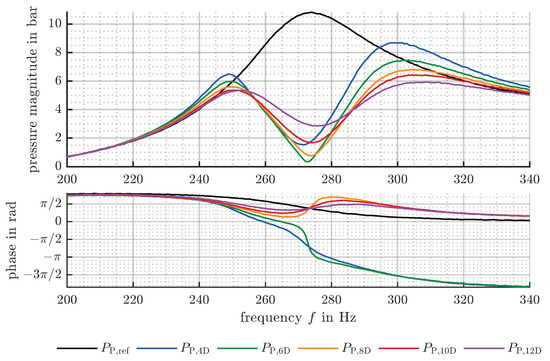
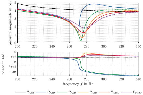
Figure 17 shows the measurement results at a mean pressure level of 100 bar with resonator pipeline, whereas Figure 18 presents the results without pipeline. Due to the dependence of the compensator stiffness on the mean pressure level, the compensation frequency decreases to 273 Hz. To match the compensation frequency with the natural frequency of the hydraulic system, the pipeline length was increased to 1.83 m. With and without pipeline, the best performance at the compensation frequency is achieved with six damping elements. The optimal damping value according to Equation (21) becomes
leading to a damping coefficient
of the compensator and a damping coefficient
per element.
Figure 17.
Measurement results for a closed pipeline with a length of 1.83 m and a mean pressure level of 100 bar. The upper plot shows the pressure magnitude and the lower plot shows the phase response. Black: system without compensator; blue: 4 damping elements; green: 6 damping elements; orange: 8 damping elements; red: 10 damping elements; purple: 12 damping elements.
Figure 18.
Measurement results without pipeline and a mean pressure level of 100 bar. The upper plot shows the pressure magnitude and the lower plot shows the phase response. Black: system without compensator; blue: 4 damping elements; green: measurement with 6 damping elements; orange: 8 damping elements; red: 10 damping elements; purple: 12 damping elements.
With resonator pipeline and six damping elements, the first harmonic of the pressure pulsation at the compensation frequency is reduced from 10.9 bar to 0.4 bar, which corresponds to a reduction rate of 96%. Without resonator pipeline, a pulsation of 4.1 bar is reduced to 0.2 bar, corresponding to a rate of 95%. Again, damping values above the optimum are preferable to insufficient damping.
7. Conclusions
This work has investigated the effectiveness of a rotary mechanical pulsation compensator for external gear pumps to reduce or cancel pressure pulsations in hydraulic systems. Under the assumption of dominant kinematic pulsation, the external gear pump is modelled in the frequency domain with flow rate and torque excitation. The model is restricted to the fundamental frequency of the pump pulsation, and nonlinear effects are neglected. In combination with a general mechanical and hydraulic system, this model has shown that the torque induced flow rate pulsation can be specifically adjusted to the flow rate excitation. The adjustment is provided in the mechanical system and is largely independent of the hydraulic system. To achieve cancellation of pressure pulsations through destructive interference, the pressure pulsations caused by the two excitations must exhibit a phase shift of relative to each other. Using the proposed rotary mechanical pulsation compensator, this phase condition can be fulfilled at the undamped natural frequency of the mechanical system. The amplitude condition is achieved through the tuning of damping. The optimal damping value, which could be calculated analytically, depends on constant pump parameters, the natural frequency of the mechanical system, and the pump outlet pressure.
Both measurements and calculations with variable pump speed have demonstrated the effectiveness of the damped rotary mechanical pulsation compensator. Two different hydraulic systems were investigated, one of which had a pronounced hydraulic resonance caused by a closed pipeline. At the natural frequency of the mechanical system and near the optimal damping value, more than 93% reduction of the first pressure pulsation harmonic was achieved in both cases. This result applies for mean pressure levels of 100 and 170 bar. Furthermore, the phase of the pressure pulsation can be used to determine whether the system is underdamped or overdamped. Both measurements and calculations showed that damping values above the optimal level are generally more favourable than insufficient damping.
The natural frequency of the mechanical system relies on the torsional stiffness of the compensator coupling, which currently depends on the transmitted torque. The next coupling design aims at constant torsional stiffness. Future work will detail the robustness of the compensator with respect to different mean pressure levels and analyse the dependencies of frequency domain bandwidth. It will be investigated if higher harmonics could be cancelled by a compensator with several degrees of freedom.
Author Contributions
Conceptualization, D.H.; methodology, D.H.; software, D.H.; validation, D.H. and G.M.; formal analysis, D.H.; investigation, D.H.; resources, G.M.; data curation, D.H.; writing—original draft preparation, D.H.; writing—review and editing, D.H. and G.M.; visualization, D.H.; supervision, G.M.; project administration, G.M. All authors have read and agreed to the published version of the manuscript.
Funding
This research received no external funding.
Data Availability Statement
The raw data are available from the corresponding author upon reasonable request.
Acknowledgments
Supported by Johannes Kepler Open Access Publishing Fund and the federal state Upper Austria.
Conflicts of Interest
The authors declare no conflicts of interest.
References
- Stosiak, M.; Karpenko, M.; Skačkauskas, P.; Deptuła, A. Identification of pressure pulsation spectrum in a hydraulic system with a vibrating proportional valve. J. Vib. Control 2024, 30, 4917–4930. [Google Scholar] [CrossRef] [Scilit]
- Ivantysyn, J.; Ivantysynova, M. Hydrostatische Pumpen und Motoren: Konstruktion und Berechnung; Vogel Fachbuch: Würzburg, Germany, 1993. [Google Scholar]
- Manring, N.D.; Kasaragadda, S.B. The Theoretical Flow Ripple of an External Gear Pump. J. Dyn. Syst. Meas. Control 2003, 125, 396–404. [Google Scholar] [CrossRef] [Scilit]
- Jiao, Z.; Chen, P.; Hua, Q.; Wang, S. Adaptive vibration active control of fluid pressure pulsations. Proc. Inst. Mech. Eng. Part I J. Syst. Control Eng. 2003, 217, 311–318. [Google Scholar] [CrossRef]
- Gao, C.; Jiang, Z.; Wang, S.; Sun, Y.; Zhang, F. Active Control of Fluid Pressure Pulsation in Hydraulic Pipe System by Bilateral-Overflow of Piezoelectric Direct-Drive Slide Valve. J. Dyn. Syst. Meas. Control 2014, 136, 031025. [Google Scholar] [CrossRef] [Scilit]
- Wang, Y.; Shen, T.; Tan, C.; Fu, J.; Guo, S. Research Status, Critical Technologies, and Development Trends of Hydraulic Pressure Pulsation Attenuator. Chin. J. Mech. Eng. 2021, 34, 14. [Google Scholar] [CrossRef] [Scilit]
- Guan, C.; Jiao, Z. Modeling and Optimal Design of 3 Degrees of Freedom Helmholtz Resonator in Hydraulic System. Chin. J. Aeronaut. 2012, 25, 776–783. [Google Scholar] [CrossRef] [Scilit]
- de Bedout, J.M.; Franchek, M.A.; Bernhard, R.J.; Mongeau, L. Adaptive-Passive Noise Control with Self-Tuning Helmholtz Resonators. J. Sound Vib. 1997, 202, 109–123. [Google Scholar] [CrossRef] [Scilit]
- Kudzma, S.; Kudzma, Z. Refined Model of Passive Branch Damper of Pressure Fluctuations. J. Theor. Appl. Mech. 2015, 53, 557–567. [Google Scholar] [CrossRef] [Scilit]
- Mikota, J.; Reiter, H. Development of a Compact and Tuneable Vibration Compensator for Hydraulic Systems. Int. J. Fluid Power 2003, 4, 17–31. [Google Scholar] [CrossRef] [Scilit]
- Mikota, G. Vorrichtung zur Reduktion von Druckpulsationen in einem Hydrauliksystem. Austrian Patent AT 526449 B1, 15 May 2024. [Google Scholar]
- Mikota, G.; Manhartsgruber, B. A Novel Pulsation Compensator for Displacement Machines. In Proceedings of the 14th International Fluid Power Conference (IFK), Dresden, Germany, 19–21 March 2024; pp. 395–406. [Google Scholar] [CrossRef] [Scilit]
- Mikota, G. Design and Simulation of a Drivetrain Integrated Pulsation Compensator for Pumps. In Proceedings of the BATH/ASME 2024 Symposium on Fluid Power and Motion Control, Bath, UK, 11–13 September 2024; pp. 1–8. [Google Scholar] [CrossRef] [Scilit]
- Holzer, D.; Mikota, G. Measurement of a Rotary Mechanical Pulsation Compensator under Hydraulic Resonance. In Proceedings of the 19th Scandinavian International Conference on Fluid Power (SICFP); River Publishers: Linköping, Sweden, 2025; pp. 139–148. [Google Scholar] [CrossRef] [Scilit]
- Mikota, G.; Holzer, D. Performance Analysis of Rotary Mechanical Pulsation Compensators for Different Types of Pumps. In Proceedings of the 15th International Fluid Power Conference (IFK), Aachen, Germany, 9–11 March 2026; pp. 741–756. [Google Scholar]
- Zhao, X.; Vacca, A. Theoretical Investigation into the Ripple Source of External Gear Pumps. Energies 2019, 12, 535. [Google Scholar] [CrossRef] [Scilit]
- Petzold, M.; Wustmann, W.; Helduser, S.; Weber, J. Analysis and Optimisation of the Pressure Reversing Process of External Gear Pumps. In Proceedings of the Fluid Power and Motion Control: FPMC 2010, Bath, UK, 15–17 September 2010; pp. 235–247. [Google Scholar]
- Holzer, D. Verfahren und Vorrichtung zur Reduktion von Druckpulsationen in einem Hydrauliksystem. Austrian Patent A 50168/2026, 2026. [Google Scholar]
- Ewins, D.J. Modal Testing: Theory, Practice and Application, 2nd ed.; Wiley: Chichester, UK, 2000. [Google Scholar]
- Beloshenko, V.; Beygelzimer, Y.; Chishko, V.; Savchenko, B.; Sova, N.; Verbylo, D.; Voznyak, A.; Vozniak, I. Mechanical properties of flexible TPU-based 3D printed lattice structures: Role of lattice cut direction and architecture. Polymers 2021, 13, 2986. [Google Scholar] [CrossRef] [Scilit] [PubMed]
- Dehen, S.; Groß, F.; Lorenz, A.; Pahr, D.H.; Reisinger, A.G. Reproducing viscoelastic properties of soft tissues in 3D printed silicone models by two-phase infill tuning. Bioprinting 2025, 48, e00408. [Google Scholar] [CrossRef] [Scilit]
- Mannesmann Rexroth. Hydraulik Komponenten: Zahnradpumpen Typ G2, Serie 4X; Technical Data Sheet RD 10 030/11.89; Mannesmann Rexroth GmbH: Lohr am Main, Germany, 1989. [Google Scholar]
- Stulemeijer, I.P.J.M. Beschreibung der Druckschwankungen in Hydrostatischen Anlagen und ihre Auswirkungen auf den Luftschall. Ph.D. Thesis, Technische Hogeschool Eindhoven, Eindhoven, The Netherlands, 1981. [Google Scholar] [CrossRef]
- D’Souza, A.F.; Oldenburger, R. Dynamic Response of Fluid Lines. Trans. ASME J. Basic Eng. 1964, 86, 589–598. [Google Scholar] [CrossRef] [Scilit]

Disclaimer/Publisher’s Note: The statements, opinions and data contained in all publications are solely those of the individual author(s) and contributor(s) and not of MDPI and/or the editor(s). MDPI and/or the editor(s) disclaim responsibility for any injury to people or property resulting from any ideas, methods, instructions or products referred to in the content. |
© 2026 by the authors. Licensee MDPI, Basel, Switzerland. This article is an open access article distributed under the terms and conditions of the Creative Commons Attribution (CC BY) license.