A Joint Fault Diagnosis and Severity Prediction Framework for Rolling Bearings Using PPCA-EMD and 1DCNN-BiGRU

Abstract

Rolling bearing fault diagnosis remains challenging due to environmental noise, insufficient information sharing between diagnosis and prediction tasks, and poor model generalization ability. To address these issues, this paper proposes a fault diagnosis and severity prediction method integrating probabilistic principal component analysis (PPCA) and empirical mode decomposition (EMD) with a one-dimensional convolutional neural network (1DCNN) and bidirectional gated recurrent unit (BiGRU). The proposed model consists of two parallel branches for fault diagnosis and fault severity prediction. A self-attention mechanism is integrated into both branches to enhance feature extraction via adaptive feature weighting. In addition, parameter sharing and weighted loss functions are adopted to improve the training efficiency and collaborative learning between the two tasks. PPCA and EMD are employed for signal denoising and reconstruction while preserving fault-related features. Experiments on public datasets and industrial production-line data show that the proposed method improves the fault classification accuracy from 92.43% to 99.71% under different load conditions, while achieving 98.99% accuracy in fault severity prediction. Noise interference tests further demonstrate the effectiveness of the model. A production-line case study further illustrates the feasibility of applying the proposed method to real monitoring signals. These results confirm the effectiveness and practical potential of the proposed method for rolling bearing fault diagnosis and health assessment.

1. Introduction

Rolling bearings are critical and vulnerable components in mechanical systems, and their health condition directly affects the operational safety and reliability of high-speed equipment [1]. During long-term high-speed operation, bearings are exposed to harsh working conditions, such as temperature fluctuations, wear, and impact loads, which gradually deteriorate their performance and eventually lead to failure. Such failures may cause unplanned downtime and economic losses and, in severe cases, may even threaten personnel safety and industrial production. Therefore, rapid and accurate fault diagnosis and condition assessment of rolling bearings are of great engineering significance [2].

With the rapid development of artificial intelligence and machine learning, these methods have been widely applied to bearing fault diagnosis and have demonstrated significant advantages. Qiu et al. [3] proposed a method combining recurrence quantification analysis (RQA), time-domain feature extraction, and a whale optimization algorithm-based support vector machine (WOA-SVM) to reduce the sensitivity of the classifier to hyperparameters. Wei et al. [4] proposed a novel imbalanced fault diagnosis framework integrating cluster-majority weighted minority oversampling technique (Cluster-MWMOTE) and a moth–flame optimization (MFO)-optimized least-squares support vector machine (LS-SVM) classifier to improve the performance of the traditional LS-SVM on complex imbalanced data and reduce its dependence on hyperparameter selection. However, machine learning-based feature extraction methods are often constrained by on-site computational resources and real-time diagnostic requirements, which restricts their practical deployment. Furthermore, these methods usually require a large amount of training data. In addition, the diagnostic accuracy of these methods strongly depends on manually designed feature parameters, which reduces their adaptability to complex nonlinear signal environments and limits their computational efficiency and cross-load performance when handling large-scale, high-dimensional data [5].

In recent years, deep learning has emerged as a promising approach for automatic feature learning in fault diagnosis because of its powerful automatic feature extraction capability [6]. Representative deep learning methods include convolutional neural networks (CNNs), recurrent neural networks (RNNs), and attention-based Transformer models. CNNs can capture local patterns with relatively few parameters, and 1DCNN models are suitable for processing one-dimensional vibration signals efficiently [7]. In addition, their better performance under the tested cross-load conditions makes them suitable for online monitoring in industrial environments [8]. Gao et al. [9] applied a 1DCNN to rolling bearing fault classification using time–frequency features of effective intrinsic mode functions (IMFs), selected by adaptive modified complementary ensemble empirical mode decomposition (AMCEEMD), as inputs, thereby improving diagnostic accuracy and reliability under noisy conditions. Ma et al. [10] applied a 1DCNN to bearing vibration time-series signals preprocessed by Fast Fourier Transform (FFT) and variational mode decomposition (VMD) bearing vibration time series signals to address the characteristics of vibration signals in fault diagnosis of rolling bearings in unmanned aerial vehicle motors.

However, traditional CNN architectures mainly focus on local feature extraction at a single scale, which limits their ability to capture multiscale temporal patterns and long-range dependencies simultaneously [11]. Recurrent neural networks and their variants, such as gated recurrent units, are well suited for long-time-series signals because of their strong capability for temporal dependency modeling. Nevertheless, they remain limited in local feature extraction, have relatively low training efficiency, and are prone to overfitting [12]. The self-attention mechanism avoids sequence-dependent recurrent structures, captures feature correlations effectively, enables efficient parallel processing and improves performance under the tested cross-load conditions. Moreover, it can be integrated into CNNs or RNNs to further improve model performance [13].

Single deep learning networks have inherent limitations in feature extraction, temporal modeling, and adaptability to varying operating conditions, making it difficult to simultaneously satisfy the requirements of local fault feature extraction and temporal evolution modeling. In contrast, hybrid network architectures can leverage the complementary strengths of different deep learning models to achieve functional complementarity and performance synergy, thereby overcoming the limitations of single networks in feature representation, temporal dependency modeling, and anti-noise capability. Zhang et al. [14] introduced a multi-modal bidirectional cross-attention fusion mechanism combined with comparative learning, which realized the precise decoupling of composite bearing faults and further demonstrated the powerful ability of deep modal interaction in complex scenarios. Yang et al. [15] designed a bidirectional cross-attention module and a multi-scale interaction network, proving that cross-modal interaction can effectively solve the feature misalignment problem and maintain high diagnostic reliability even in extremely low-signal-to-noise-ratio (SNR) environments. Xu et al. [16] proposed a fusion method integrating feature mode decomposition (FMD)–Continuous Wavelet Transform (CWT) and Hybrid Pooling–Residual Network model (Hybrid Pooling–ResNet, HP-ResNet), which effectively overcomes incomplete feature extraction and limited classification accuracy in traditional methods while achieving strong performance under the tested cross-load conditions. Wu et al. [17] demonstrated that Gradient-weighted Class Activation Mapping (Grad-CAM) can map the attention weights of CNN models to specific time points and sensor channels, thereby enhancing model interpretability and diagnostic reliability.

In practical industrial scenarios, bearing vibration signals collected under varying operating conditions and load levels are often heavily contaminated by noise, which may obscure the weak impact signals associated with incipient faults [18]. Therefore, signal denoising is essential for bearing fault diagnosis and for deriving health scores [19]. Shen et al. [20] proposed a method to improve weak fault feature extraction and fault diagnosis accuracy. Li et al. [21] optimized the VMD method to overcome the limitations of traditional VMD, including its reliance on predetermined parameters and the difficulty of selecting optimal IMFs. Nevertheless, existing denoising methods still suffer from difficult parameter tuning, high computational complexity, and the loss of critical features. PPCA, which explicitly models data uncertainty, can effectively suppress background noise while preserving weak fault-related features, making it particularly advantageous for early bearing fault diagnosis. Xiang et al. [22] verified the effectiveness of PPCA in removing background noise and preserving weak fault features in bearing fault diagnosis.

In summary, deep learning-based methods for bearing fault diagnosis have made considerable progress. However, existing studies still face several challenges. First, a single-network architecture is generally insufficient to simultaneously capture the associations between local spatial features and global long-term temporal features. Moreover, most existing hybrid models are primarily designed to improve the accuracy of a specific task and are generally limited to single-task diagnosis; therefore, their capability for multitask diagnosis remains limited. Second, vibration signals collected from faulty bearings in practical applications are often contaminated by background noise. Therefore, maintaining high fault diagnosis accuracy under strong noise conditions remains an issue that requires further investigation. Finally, the effectiveness and applicability of current algorithms in real-world engineering scenarios warrant further validation using industrial data.

To address the above limitations, this paper designs a task-oriented integrated framework for fault diagnosis that combines signal denoising and adaptive reconstruction with joint fault classification and severity prediction. Specifically, PPCA is first used to denoise the raw signal, after which EMD is applied to extract effective intrinsic mode function components for signal reconstruction. The reconstructed signal is then fed into the hybrid 1DCNN-BiGRU model for fault identification and health assessment. Experimental results show that the proposed method preserves useful signal components, suppresses noise, and improves diagnosis and severity prediction accuracy in the tested scenarios. Furthermore, we compare various cross-load adaptation methods across different datasets to further validate the effectiveness of the proposed method under varying working conditions. In practical application scenarios, the proposed method achieves accurate fault diagnosis.

The main contributions of this study are as follows:

• A hybrid denoising and signal reconstruction strategy is proposed. This strategy combines the global denoising capability of PPCA with the adaptive signal decomposition advantage of EMD. The signal is decomposed into IMFs at different scales, and effective components are selected for reconstruction. In this way, environmental noise is suppressed while nonstationary fault-induced impact features are preserved, thereby providing high-quality input data for subsequent models.
• A hybrid model for parallel feature extraction and temporal learning is constructed. In this model, the 1DCNN extracts key local features from the reconstructed signal, whereas the BiGRU captures temporal correlation information, thereby overcoming the limitation of traditional CNNs in modeling contextual dependencies in sequential signals. In addition, a self-attention mechanism is introduced to adaptively concentrate on features with higher contributions to diagnosis and prediction.
• The model’s generalization capability and adaptability to limited-sample conditions are improved. By freezing selected model layers, efficient learning under limited-sample conditions is achieved. The model trained on public datasets maintains excellent performance when transferred to fault diagnosis of actual production-line signals, which further validates its generalization capability and supports its practical deployment in industrial rolling bearing health management.

2. Methodology

2.1. PPCA Denoising

This module is designed to achieve global denoising of the input signal while preserving fault-related feature components as much as possible. PPCA is a probabilistic extension of principal component analysis (PCA). Specifically, PPCA projects high-dimensional noisy observations into a low-dimensional latent subspace through a generative probabilistic model and reconstructs the data from this subspace to filter out noise [23]. Compared with wavelet denoising and related methods, PPCA can automatically estimate the noise level without manual intervention while simultaneously reducing data dimensionality, thereby facilitating the training of subsequent deep learning models. The PPCA model first assumes that the observed data satisfy the following relationship:

$$\mathit{X}=\mathit{P}·\mathit{u}+\mathit{E}$$

(1)

where $\mathit{X}=\{{\mathit{X}}_1,{\mathit{X}}_2,\dots ,{\mathit{X}}_m\}\in {\mathbb{R}}^{n\times m}$ is an $n\times m$ matrix; n is the number of original variables; and m is the number of samples. $\mathit{P}$ is the $n\times k$ transformation matrix from a low-dimensional space to a high-dimensional space and k is the number of principal components. The $k\times m$ matrix $\mathit{u}=\{{\mathit{u}}_1,{\mathit{u}}_2,\dots ,{\mathit{u}}_m\}\in {\mathbb{R}}^{k\times m}$ is the principal component matrix and is assumed to follow a Gaussian distribution with zero mean and covariance $\mathit{I}$. $\mathit{E}$ is an isotropic Gaussian noise matrix satisfying $N(\mathbf{0},{\sigma }^2\mathit{I})$, where ${\sigma }^2$ denotes the variance parameter of the noise variable. Therefore, $\mathit{X}$ follows $N(\mathbf{0},\mathit{P}{\mathit{P}}^{\mathrm{T}}+{\sigma }^2\mathit{I})$.

The principal component variables are assumed to follow this probability distribution:

$$p\left(\mathit{u}\right)={\left(2\pi \right)}^{-{\displaystyle \frac{k}{2}}}exp\left\{-{\displaystyle \frac{1}{2{\sigma }^2}}{\mathit{X}}^{\mathrm{T}}\mathit{X}\right\}$$

(2)

The conditional probability distribution over x-space for a given $\mathit{u}$ is:

$$p\left(\mathit{X}|\mathit{u}\right)={\left(2\pi \right)}^{-{\displaystyle \frac{n}{2}}}exp\left\{-{\displaystyle \frac{1}{2{\sigma }^2}}{∥\mathit{X}-\mathit{P}·\mathit{u}∥}^2\right\}$$

(3)

Combining Equations (2) and (3) yields the marginal probability distribution of the original variables, which is expressed as follows:

$$p\left(\mathit{X}\right)=\int p\left(\mathit{u}\right)p\left(\mathit{X}|\mathit{u}\right)d\mathit{X}={\left(2\pi \right)}^{-{\displaystyle \frac{n}{2}}}{\left|\mathit{C}\right|}^{-{\displaystyle \frac{1}{2}}}exp\left\{-{\displaystyle \frac{1}{2}}{\mathit{X}}^{\mathrm{T}}{\mathit{C}}^{-1}\mathit{X}\right\}$$

(4)

where $\mathit{C}=\mathit{P}{\mathit{P}}^{\mathrm{T}}+{\sigma }^2\mathit{I}$ is an $n\times n$ covariance matrix determined by $\mathit{P}$ and ${\sigma }^2$.

According to Bayes’ theorem, the posterior probability distribution of the principal component variables given the original variables is expressed as follows:

$$p\left(\mathit{u}|\mathit{X}\right)={\left(2\pi \sigma \right)}^{-{\displaystyle \frac{k}{2}}}{\left|{\sigma }^{-2}\mathit{M}\right|}^{{\displaystyle \frac{1}{2}}}exp\left\{-{\displaystyle \frac{1}{2}}{\left[\mathit{u}-{\mathit{M}}^{-1}{\mathit{P}}^{\mathrm{T}}{\mathit{X}}^{\mathrm{T}}\right]}^{\mathrm{T}}\left({\sigma }^{-2}\mathit{M}\right)\left[\mathit{u}-{\mathit{M}}^{-1}{\mathit{P}}^{\mathrm{T}}\mathit{X}\right]\right\}$$

(5)

where $\mathit{M}={\mathit{P}}^{\mathrm{T}}\mathit{P}+{\sigma }^2\mathit{I}$ is a $k\times k$ matrix.

The iterative update expressions for the transformation matrix $\mathit{P}$ and the noise variance ${\sigma }^2$ can be derived using the Expectation-Maximization (EM) algorithm for classical parameter estimation of the latent variable model, as follows:

$$\mathit{P}=\mathit{S}\mathit{P}{\left({\sigma }^2\mathit{I}+{\mathit{M}}^{-1}{\mathit{P}}^{\mathrm{T}}\mathit{S}\mathit{P}\right)}^{-1}$$

(6)

$${\sigma }^2={\displaystyle \frac{1}{n}}tr\left(\mathit{S}-\mathit{S}\mathit{P}{\mathit{M}}^{-1}{\mathit{P}}^{\mathrm{T}}\right)$$

(7)

where $\mathit{S}$ is the covariance matrix of the observed data and $tr\left(·\right)$ represents the trace of the matrix.

The two parameters $\mathit{P}$ and ${\sigma }^2$ are calculated through multiple iterations. Once ${\sigma }^2$ and $\mathit{P}$ are obtained, the PPCA model can be established to derive the data of each principal component. When the PPCA model is constructed, the denoising model will be obtained using the following transformation:

$${\mathit{u}}_i={\mathit{P}}_i^T\mathit{X}$$

(8)

As shown in Equation (8), each principal component is the projection from the raw data $\mathit{X}$ to the corresponding principal component vector ${\mathit{P}}_i$. Finally, the PPCA denoising model with reduced matrix dimensionality is obtained and the raw signal is denoised.

Regarding dimensionality selection, when the cumulative contribution rate reaches or exceeds 95%, only the first s eigenvectors are selected as sample features. This setting is intended to preserve the principal information while reducing feature redundancy.

2.2. Principle of the EMD Algorithm

Empirical mode decomposition, proposed by Huang et al, is an adaptive signal processing method for nonlinear and nonstationary signal analysis. It decomposes a complex signal into a finite set of intrinsic mode functions with different characteristic scales and a residual term representing the underlying trend. Unlike conventional signal analysis methods, such as the Fourier transform and wavelet transform, which rely on predefined basis functions, EMD performs decomposition entirely on the basis of the intrinsic time–frequency characteristics of the signal, thus offering strong adaptability and broad applicability [24]. The main implementation steps of the EMD algorithm are as follows [25]:

• Identify all extrema: Determine all local maxima and minima of the original vibration signal;
• Construct the envelope curves: Apply cubic spline interpolation to all local maxima to obtain the upper envelope $E_{max}\left(t\right)$, and to all local minima to obtain the lower envelope $E_{min}\left(t\right)$;
• Calculate the mean envelope: Compute the mean of the upper and lower envelopes as follows:

  $$A_1\left(t\right)={\displaystyle \frac{E_{max}\left(t\right)+E_{min}\left(t\right)}{2}}$$

  (9)
• Obtain the intermediate signal: Subtract the mean envelope $A_1\left(t\right)$ from the original signal $S\left(t\right)$ to obtain the intermediate signal $D_1\left(t\right)$:

  $$D_1\left(t\right)=S\left(t\right)-A_1\left(t\right)$$

  (10)
• Check the IMF criteria: Determine whether the intermediate signal $D_1\left(t\right)$ satisfies the following two conditions for an IMF.

A component is regarded as an IMF when it satisfies two conditions. First, over the whole signal, the number of extrema and the number of zero crossings must be equal or differ by at most one. Second, the local mean value of the upper and lower envelopes should be approximately zero at any time instant. If the intermediate signal satisfies these two conditions, it is identified as an IMF; otherwise, the sifting process is repeated.

If $D_1\left(t\right)$ satisfies the above conditions, it is identified as the first IMF component of the original signal. Otherwise, $D_1\left(t\right)$ is treated as the new original signal, and Steps 1–5 are repeated until the IMF criteria are satisfied. The extracted IMF component is then subtracted from the original signal $S\left(t\right)$ to obtain a new residual signal. This decomposition process is repeated on the residual signal until it becomes a monotonic function that can no longer be decomposed into additional IMF components. According to the above decomposition procedure, the original signal $S\left(t\right)$ can be expressed as the sum of all IMF components and the final residual term:

$$S\left(t\right)={\displaystyle \sum _{n=1}^k}IM{F}_n\left(t\right)+r_o\left(t\right)$$

(11)

where k denotes the number of IMF components obtained by decomposition, and $r_o\left(t\right)$ denotes the residual term of the signal.

Although standard EMD is adaptive, it may suffer from mode mixing, endpoint effects, and noise sensitivity. In this study, these issues are alleviated by combining PPCA denoising with EMD-based signal reconstruction. During EMD, cubic spline interpolation is used to construct the upper and lower envelopes, and mirror-symmetric boundary extension is applied at both endpoints before envelope interpolation to reduce endpoint distortion. The sifting stopping threshold is set to 0.25, and the maximum number of IMFs is limited to 12 to control computational cost.

2.3. 1DCNN Model

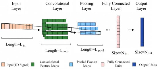
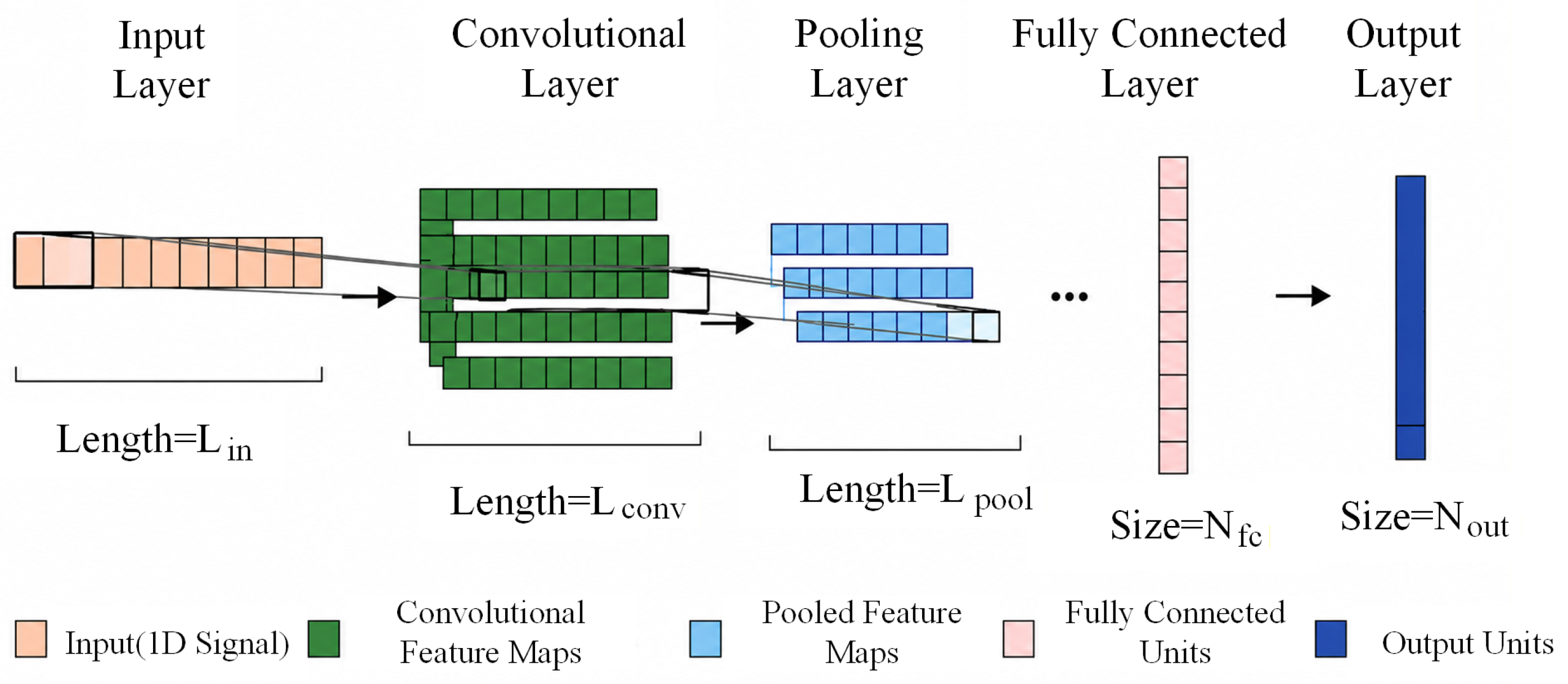
A one-dimensional convolutional neural network is a classical feedforward deep learning model [26]. It primarily consists of convolutional layers, pooling layers, activation functions, and fully connected layers, which are used to extract and transform features from input data. In classification tasks, the fully connected layer integrates the extracted features and maps them to specific categories or labels. As shown in Figure 1, the model consists of multiple artificial neurons and a classifier. Through the interaction among neurons, the model learns discriminative fault-related representations from the input signals and extracts latent features that characterize the fault states of rolling bearings, which are subsequently fed into the classifier for fault identification [27]. By alternately stacking convolutional and pooling layers, the 1DCNN progressively captures multiscale local features from bearing vibration signals, thereby providing reliable support for subsequent fault identification tasks [28].

Figure 1. Typical architecture of the 1DCNN model.

2.4. BiGRU-Based Health Assessment Model

The bidirectional gated recurrent unit network integrates two gated recurrent unit (GRU) modules for forward and backward propagation, thereby effectively utilizing both past and future information and capturing bidirectional temporal dependencies in time-series data [29]. In addition, the BiGRU network employs a gating mechanism to selectively retain or discard temporal information, which enables more accurate modeling of the temporal evolution of bearing vibration signals. Because bearing vibration signals vary over time, health state prediction depends not only on the current vibration condition but also on historical states and temporal trends [30]. By effectively capturing such long-term dependencies, the BiGRU network supports more accurate assessment of bearing health status.

2.5. Design of the Self-Attention Mechanism

Integrating an attention mechanism into the network enables the model to better capture correlations among temporal features and to adaptively emphasize informative feature representations [31]. The attention mechanism operates by introducing learnable weights that allow the model to dynamically assign different levels of importance to different input elements. This adaptive weighting strategy enables the model to process input data more efficiently and capture feature correlations more accurately [32].

To focus on critical fault features, a multi-head self-attention mechanism is integrated. Given the hidden state sequence $H\in {\mathbb{R}}^{B\times T\times d}$ from the BiGRU (where $B=64$ is the batch size, $T=128$ is the number of time steps, and $d=256$ is the feature dimension), the attention function is defined as follows:

$$Attention\left(Q,K,V\right)=softmax\left({\displaystyle \frac{Q{K}^T}{\sqrt{d_K}}}\right)V$$

(12)

where Q, K and V represent the query matrices, key matrices, and value matrices, respectively, obtained by linearly transforming the input feature matrix; $d_K$ denotes the dimension of the key matrix K; $d_K$ serves as a scaling factor to prevent the inner product of Q and K from becoming excessively large and causing saturation of the $softmax$ function; and the $softmax\left(·\right)$ function is used to normalize the weights of different features to $\left[0, 1\right]$.

In this study, we employ a 4-head attention structure $(h=4)$, and the outputs of all heads are concatenated and projected to form the final enhanced feature representation.

2.6. Fault Diagnosis and Health Assessment Model

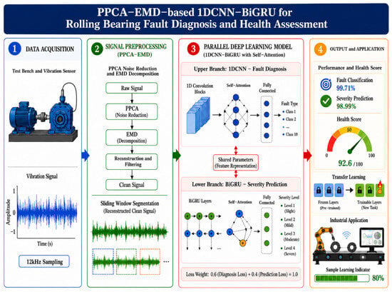
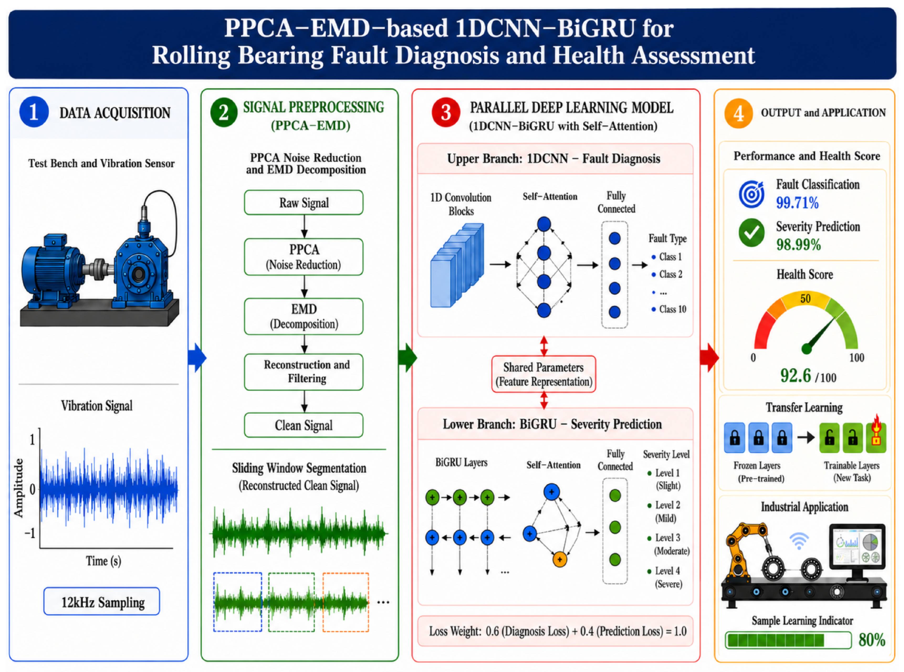
The proposed method is a preprocessing-assisted multitask diagnosis framework. The raw continuous vibration signals are first divided into mutually exclusive training and validation subsets. Signal segmentation, denoising, decomposition, reconstruction, and model training are then performed according to this predefined split to avoid information leakage. The overall framework consists of three main stages: signal preprocessing, fault diagnosis and severity prediction, and output of diagnosis and assessment results. The corresponding flowchart is shown in Figure 2.

Figure 2. Flowchart of 1DCNN and BiGRU fault diagnosis and evaluation model based on PPCA-EMD.

The specific procedure is described as follows:

• Signal preprocessing stage: The raw continuous vibration signals are first divided into training and validation subsets at the raw signal file or continuous time block level to avoid information leakage. Sliding-window segmentation is then performed independently within each subset to generate fixed-length samples. The normalization parameters and PPCA projection parameters are estimated only from the training subset and then applied to the validation subset. Subsequently, the denoised signals are decomposed by EMD, and the effective IMF components are selected for signal reconstruction.
• Fault diagnosis and severity prediction stage: The reconstructed samples are fed into the 1DCNN-BiGRU-Self-Attention network. The 1DCNN blocks extract local fault-related features, the stacked BiGRU layers model bidirectional temporal dependencies, and the self-attention module adaptively weights informative temporal features. The shared representation is then passed to two task-specific branches for fault classification and severity prediction. The model is trained using a weighted multitask loss function.
• Diagnosis and assessment output stage: This stage outputs the fault classification and fault severity prediction results of all validation samples in the form of confusion matrices, thereby enabling quantitative evaluation of the diagnostic and predictive performance of the proposed model. In addition, selected pretrained layers can be frozen to support subsequent limited-sample transfer experiments under cross-load conditions.

3. Experimental Analysis

3.1. Vibration Data Processing

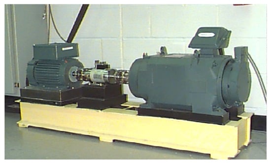
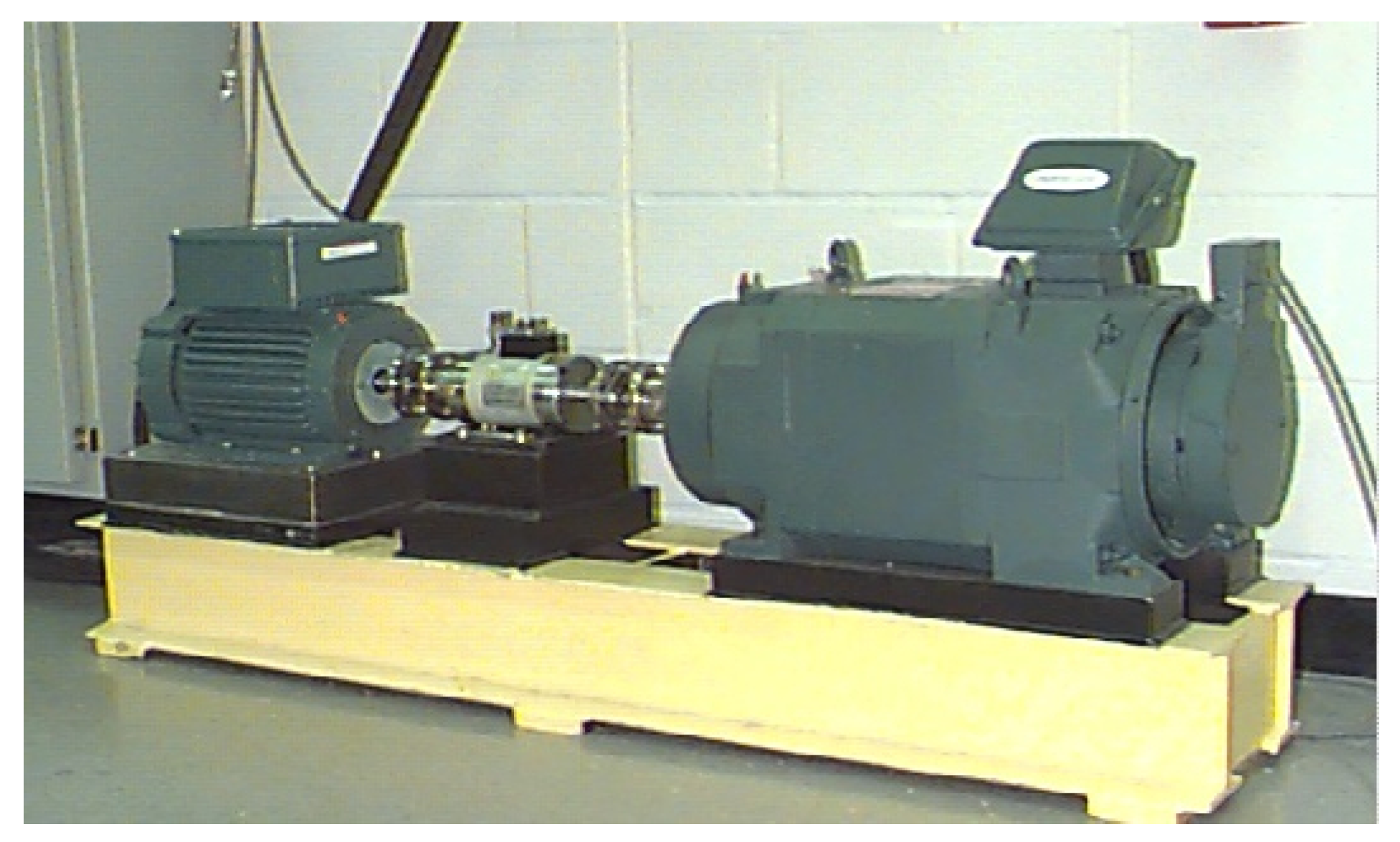
1. The experimental dataset used in this study is the public rolling bearing fault dataset collected by Case Western Reserve University (CWRU) using a dedicated bearing fault test rig, as shown in Figure 3 [33]. This dataset has been widely used in rolling bearing fault diagnosis studies for model validation and performance comparison. The test rig consists of a motor, a torque sensor, a coupling, and a bearing housing.

Figure 3. The CWRU bearing failure experiment platform.

The collected data (12k Drive-End Bearing Fault Data) are vibration signals acquired from the drive-end bearing during operation at a sampling frequency of 12 kHz. The dataset contains three fault location categories. Each fault category includes three fault sizes and four load levels. The fault sizes are 0.007, 0.014, and 0.021 inch, and the load levels are 0 hp (motor speed: 1797 r/min), 1 hp (1772 r/min), 2 hp (1750 r/min), and 3 hp (1730 r/min), as presented in Table 1.

Table 1. Classification details of the CWRU bearing dataset.

Motor Load	Fault Type	Damage Diameter	Label	Training Samples	Validation Samples
0/1/2/3 hp	Normal	-	0	163	70
	Inner Race Fault	0.007 inch	1	163	70
	Ball Fault	0.007 inch	2	163	70
	Outer Race Fault	0.007 inch	3	163	70
	Inner Race Fault	0.014 inch	4	163	70
	Ball Fault	0.014 inch	5	163	70
	Outer Race Fault	0.014 inch	6	163	70
	Inner Race Fault	0.021 inch	7	163	70
	Ball Fault	0.021 inch	8	163	70
	Outer Race Fault	0.021 inch	9	163	70

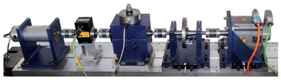
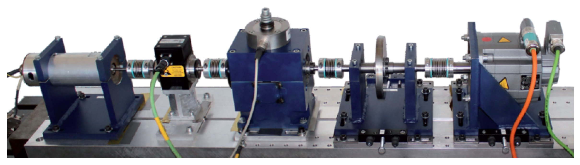
2. To further evaluate the cross-load performance of the proposed method, the Paderborn University (PU) bearing dataset from Germany is introduced as an external validation dataset. As shown in Figure 4, the experimental platform consists of a 425 W servo motor, a torque-measuring shaft, a rolling bearing test module, and a load motor. The tested bearings are 6203 deep-groove ball bearings. Differently from artificially induced faults, the PU dataset contains bearing damage generated through accelerated life tests, including samples with real pitting and spalling defects. Therefore, its vibration signals exhibit stronger nonstationarity and weaker impulse characteristics, making the dataset more suitable for evaluating the adaptability of the model under realistic fault conditions.

Figure 4. Mechanical setup of the PU dataset test rig.

In this study, a cross-condition transfer experiment is designed based on different operating loads. The source domain is defined as condition N15M07, corresponding to a rotational speed of 1500 r/min and a torque load of 0.7 Nm, and is used for model training. The target domain is defined as condition N15M01, corresponding to the same rotational speed of 1500 r/min but a lower torque load of 0.1 Nm, and is used directly for validation. The classification task includes five categories, namely healthy bearings, artificially damaged bearings, and bearings with real fatigue damage, as listed in Table 2.

Table 2. Label definitions of the PU bearing dataset.

Fault Type	Label	Training Samples	Validation Samples
Normal	0	500	200
Artificial Outer	1	500	200
Artificial Inner	2	500	200
Real Fatigue Outer	3	500	200
Real Fatigue Inner	4	500	200

To demonstrate the operational workflow of the proposed model, the CWRU bearing dataset is adopted as an illustrative example. The preprocessing steps applied to the raw vibration signals are detailed as follows:

• Signal sampling and labeling. For each bearing condition in the dataset, the first 10 s of vibration data are selected, corresponding to 120,000 data points for each bearing condition. Each raw signal file is assigned a condition label according to the predefined labeling rules, and the meaning of each digit is presented in Table 3.

  Table 3. Naming rules for original sample labels.

  Serial Number/Label	0	1	2	3
  First digit (Damage size/inch)	Normal	0.007	0.014	0.021
  Second digit (Load/hp)	0	1	2	3
  Third digit (Damage type)	None	Ball	Inner race	Outer race

  Table 3. Naming rules for original sample labels.

  Serial Number/Label	0	1	2	3
  First digit (Damage size/inch)	Normal	0.007	0.014	0.021
  Second digit (Load/hp)	0	1	2	3
  Third digit (Damage type)	None	Ball	Inner race	Outer race

• Sliding-window segmentation and time-series labeling. The training and validation subsets are divided at a ratio of 7:3, corresponding to 70% and 30% of the raw signal blocks, respectively. Based on the original labeling rules, new time-series labels are assigned according to the predefined renaming scheme, as shown in Table 4.

  Table 4. Structure of the renamed sample label.

  Label Bits	Field Code	Description
  1–2	DS	Damage size
  3–4	LL	Load level
  5–6	FT	Fault type
  7–9	TSI	Time series index

  Table 4. Structure of the renamed sample label.

  Label Bits	Field Code	Description
  1–2	DS	Damage size
  3–4	LL	Load level
  5–6	FT	Fault type
  7–9	TSI	Time series index

• PPCA denoising and EMD-based signal reconstruction. The obtained samples with time-series labels are first denoised by PPCA and then decomposed by EMD. Signal reconstruction is subsequently performed based on the correlation coefficients of the IMF components. The number of retained PPCA components is automatically selected based on the criterion that the cumulative variance contribution rate reaches 95%. The EMD procedure follows the settings described in Section 2.2, and IMF components with cross-correlation coefficients greater than 0.3 are selected as effective components for signal reconstruction.
• Sample set organization. The reconstructed signal samples are organized into the input format required by the 1DCNN-BiGRU model, namely (number of samples, signal length, number of channels), which is (9320, 1024, 1) in this study.

The cross-correlation coefficient serves as an indicator of the relevance and effectiveness of each IMF component. Specifically, coefficients in the ranges of 0–0.3, 0.3–0.5, 0.5–0.8, and 0.8–1 indicate weak, moderate, significant, and high correlation, respectively. IMF components with weak correlation are regarded as spurious components containing little useful fault information. Based on a portion of the CWRU dataset, boundary extension and EMD are first performed on the vibration samples to obtain multiple IMF components. The distribution of the retained IMF components is then statistically analyzed over the evaluation samples. Among the 2330 samples from the Case Western Reserve University dataset, 72.62% selected one IMF component, 22.15% selected two IMF components, and 5.23% selected three or more IMF components. Since PPCA has already been applied to suppress global noise, the IMF selection strategy used for EMD-based reconstruction has only a minor influence on the accuracy of the proposed method.

3.2. Experimental Environment and Key Model Architecture

The experiments are conducted on a computer equipped with an AMD (Santa Clara, CA, USA) Ryzen 7 3750H processor and an NVIDIA (Santa Clara, CA, USA) GeForce RTX 1650 graphics processing unit (GPU). The software environment is configured using Anaconda, and Python 3.10 is used as the main programming language. The proposed deep learning model is implemented using TensorFlow/Keras. To further improve reproducibility, the key architecture and training parameters of the proposed multitask neural network are summarized in Table 5.

Table 5. Key architecture and training parameters of the proposed 1DCNN-BiGRU-Attention model.

Parameter	Value	Description
input_shape	$1024\times 1$	Input size of each reconstructed vibration signal sample
batch_size	64	Batch size used for model training
optimizer	Adam	Optimizer used for model optimization
learning_rate	0.001	Initial learning rate of the Adam optimizer
epochs	150	Maximum number of training epochs
conv_filters	64, 128, 256	Number of filters in the three 1DCNN layers
conv_kernel_size	8, 4, 2	Kernel sizes of the three 1DCNN layers
max_pool_size	2	Pooling size of each one-dimensional max-pooling layer
cnn_dropout	0.2, 0.2, 0.3	Dropout rates after the three CNN blocks
bigru_layers	2	Number of stacked bidirectional GRU layers
bigru_units	128	Number of GRUs in each direction
attention_heads	4	Number of heads in the self-attention module
attention_key_dim	64	Key dimension of each attention head
loss_weight	0.6 and 0.4	Loss weights for fault classification and severity prediction, respectively
L2_regularization	$1\times {10}^{-4}$	L2 regularization coefficient used in trainable layers
early_stopping_patience	25	Number of epochs without validation-loss improvement before early stopping

The proposed 1DCNN-BiGRU-Attention model has approximately 1.4 million parameters and requires 72.0 M floating-point operations (FLOPs) per inference cycle. On the NVIDIA RTX 1650 GPU, the inference time of each sample is 160.4 ms, which meets the common industrial real-time monitoring needs. Although the number of parameters is slightly higher than that of the baseline models (e.g., 1DCNN 0.52 M), its inference speed is still acceptable on mainstream edge devices, showing the potential for actual deployment. Future work can further reduce the model size using compression techniques.

The proposed network is optimized using a weighted multitask loss function. For both the fault classification task and the fault severity prediction task, weighted sparse categorical cross-entropy is adopted to reduce the influence of class imbalance. For a task $q\in \{f,s\}$, where f denotes fault classification and s denotes severity prediction, the loss function is defined as:

$${\mathcal{L}}_q=-{\displaystyle \frac{1}{N_q}}{\displaystyle \sum _{i=1}^{N_q}}{w}_{y_i^q}^{q}log\left(p_{i,y_i^q}^q\right)$$

(13)

where $N_q$ is the number of training samples for task q, $y_i^q$ is the true label of the i-th sample for task q, $p_{i,y_i^q}^q$ is the predicted probability corresponding to the true class, and $w_{y_i^q}^q$ is the class weight of the corresponding class. The class weights are calculated only from the training set using a balanced weighting strategy:

$$w_{y_i^q}^q={\displaystyle \frac{N_q}{K_q{N}_c^q}}$$

(14)

where $K_q$ is the number of classes in task q, and $N_c^q$ is the number of training samples belonging to class c in task q.

The total multitask loss is expressed as:

$${\mathcal{L}}_{total}={\lambda }_f{\mathcal{L}}_f+{\lambda }_s{\mathcal{L}}_s+\beta {\parallel \Theta \parallel }_2^2$$

(15)

where ${\mathcal{L}}_f$ and ${\mathcal{L}}_s$ are the fault classification loss and fault severity prediction loss, respectively; ${\lambda }_f$ and ${\lambda }_s$ are the corresponding task weights; $\Theta$ denotes the trainable parameters of the network; and $\beta$ is the L2 regularization coefficient. According to Liu et al. [34], in their study on multitask fault diagnosis of wheelset bearings, a grid search over the loss weights showed that the weight combination of 0.6 and 0.4 achieved the optimal fault diagnosis performance. This finding indicates that, in multitask learning for mechanical fault diagnosis, assigning unequal weights can effectively balance the contributions of the main task and the related auxiliary task. Therefore, this study adopts ${\lambda }_f=0.6$ and ${\lambda }_s=0.4$ as the loss weights for fault diagnosis and degradation degree prediction, respectively.

3.3. Validation and Result Analysis of Fault Diagnosis and Severity Prediction

To evaluate the superiority of the proposed PPCA-EMD-1DCNN-BiGRU model, comparative experiments are conducted with a 1DCNN-Transformer model [35], a Wide First-Layer Kernel Deep Convolutional Neural Network (WDCNN) model [36], a convolutional neural network–long short-term memory (CNN-LSTM) model [37], and an Efficient Convolutional Transformer (ECTN) [38]. The raw vibration signals are first segmented using the same window-generation protocol and then processed by the same PPCA denoising, EMD, correlation-based IMF selection, and signal reconstruction procedure. The reconstructed signals are used as the input of the proposed model and all deep learning baseline models. The fault diagnosis accuracies of the different models under fixed load conditions are summarized in Table 6.

Table 6. Accuracy comparison of different methods under different load conditions on the CWRU dataset (%).

Load/Method	ECTN	1DCNN-Transformer	WDCNN	CNN-LSTM	The Proposed Method
0 hp	96.48 ± 0.32	95.34 ± 0.44	99.97 ± 0.05	97.82 ± 0.69	99.99 ± 0.01
1 hp	97.18 ± 0.08	92.48 ± 0.21	99.33 ± 0.45	97.18 ± 0.43	99.86 ± 0.07
2 hp	96.04 ± 0.13	93.19 ± 0.47	99.19 ± 0.28	95.87 ± 2.07	99.57 ± 0.09
3 hp	91.62 ± 1.12	88.71 ± 0.19	97.35 ± 0.98	97.46 ± 0.65	99.41 ± 0.12
Mean	95.33	92.43	98.96	97.08	99.71

As shown in Table 6, the compared methods can be ranked in terms of average fault diagnosis accuracy as follows: 1DCNN-BiGRU-Attention, WDCNN, CNN-LSTM, ECTN and CNN-Transformer. All deep learning-based models achieved relatively high fault recognition accuracy in bearing fault diagnosis. In particular, the proposed model achieved the highest mean accuracy of 99.71%, indicating that the combined 1DCNN-BiGRU structure improved classification performance under the same preprocessing pipeline.

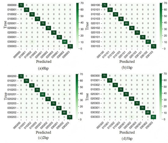
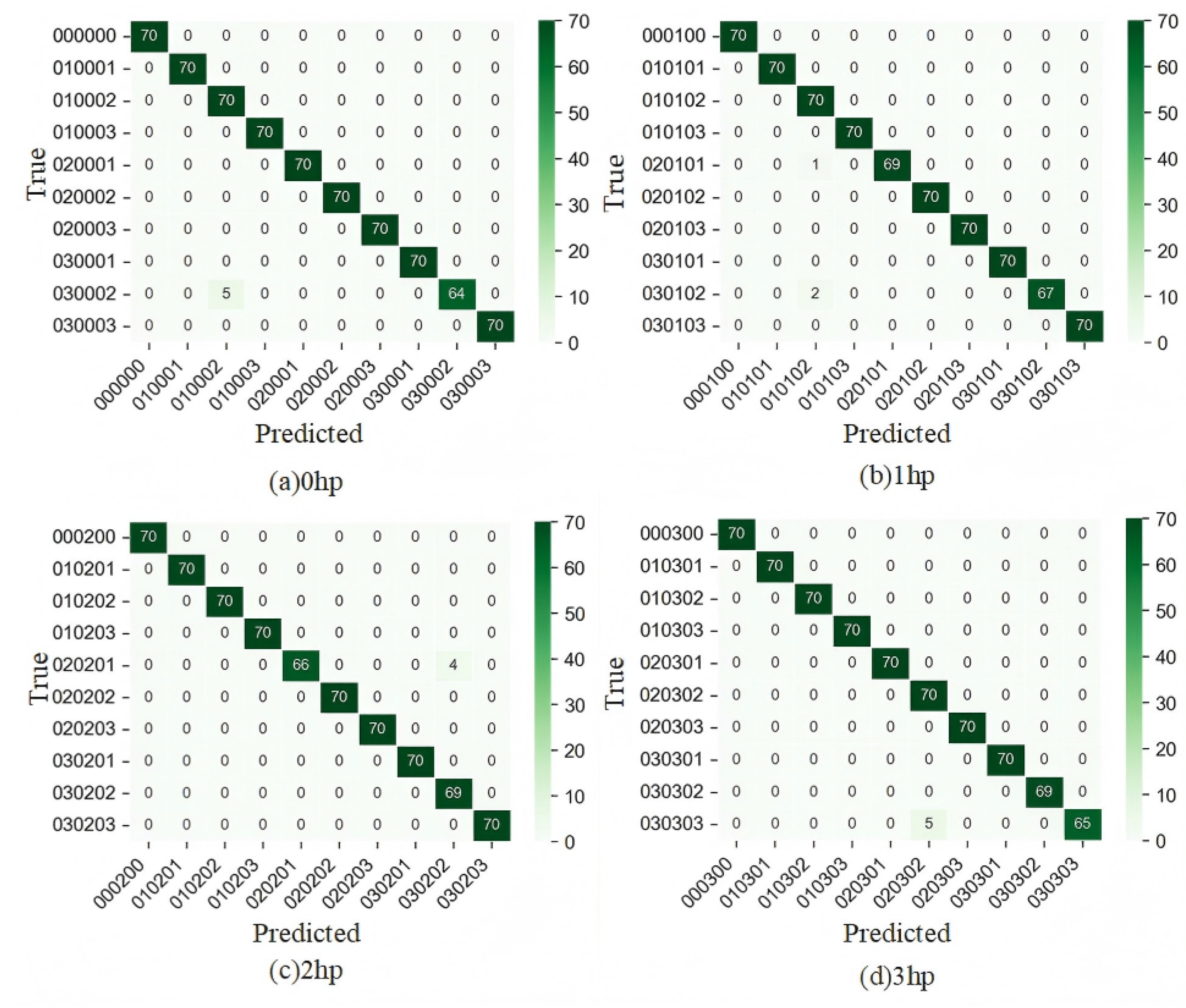
The confusion matrices (CMs) for fault classification under the four load conditions are shown in Figure 5. The results indicate that most validation samples are correctly classified along the diagonal, demonstrating stable fault-type identification under fixed-load conditions. For the 0 hp, 1 hp, 2 hp, and 3 hp cases, only a small number of samples are misclassified between fault categories with similar fault diameters or fault locations. This suggests that the proposed model can extract discriminative fault-related features from the reconstructed vibration signals and maintain high classification consistency across different load levels.

Figure 5. Confusion matrices for fault classification across different load conditions on the CWRU dataset.

To evaluate the health condition of rolling bearings more robustly, both the instantaneous degradation degree and the historical degradation trend are considered. The instantaneous health score is first calculated according to the state deviation from the health baseline. Following the health mapping strategy based on the Mahalanobis distance and reliability correction [39], the instantaneous health score at time t is defined as

$$H{S}_t=100exp\left(-\epsilon ·{\displaystyle \frac{d({\mathit{X}}_{obs,t},{\mathit{X}}_{est,t})}{T}}\right)$$

(16)

where $H{S}_t$ denotes the instantaneous health score at time t; $d({\mathit{X}}_{obs,t},{\mathit{X}}_{est,t})$ represents the Mahalanobis distance between the observed state vector ${\mathit{X}}_{obs,t}$ and the estimated health baseline ${\mathit{X}}_{est,t}$; T is the average deviation threshold of normal data; and $\epsilon$ is the sensitivity coefficient.

Since bearing degradation is a continuous time-dependent process, the health score at a single time instant may be affected by local fluctuations or measurement noise. Therefore, an exponentially weighted moving average (EWMA)-based auxiliary score is introduced to incorporate historical health information [40]. The time-series-assisted health score is expressed as:

$$H{S}_t^{ts}=\mu H{S}_t+(1-\mu )H{S}_{t-1}^{ts}$$

(17)

where $H{S}_t^{ts}$ denotes the time-series-assisted health score at time t, and $H{S}_{t-1}^{ts}$ is theis the auxiliary health score at the previous time step. The initial value is set as $H{S}_0^{ts}=H{S}_0$. The parameter $\mu \in [0, 1]$ is the smoothing coefficient. A larger $\mu$ assigns greater importance to the current health state, whereas a smaller $\mu$ increases the contribution of historical health information.

Finally, the instantaneous health score and the time-series-assisted health score are fused to obtain the comprehensive health score:

$$H{S}_t^{final}=\lambda H{S}_t+(1-\lambda )H{S}_t^{ts}$$

(18)

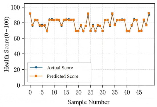
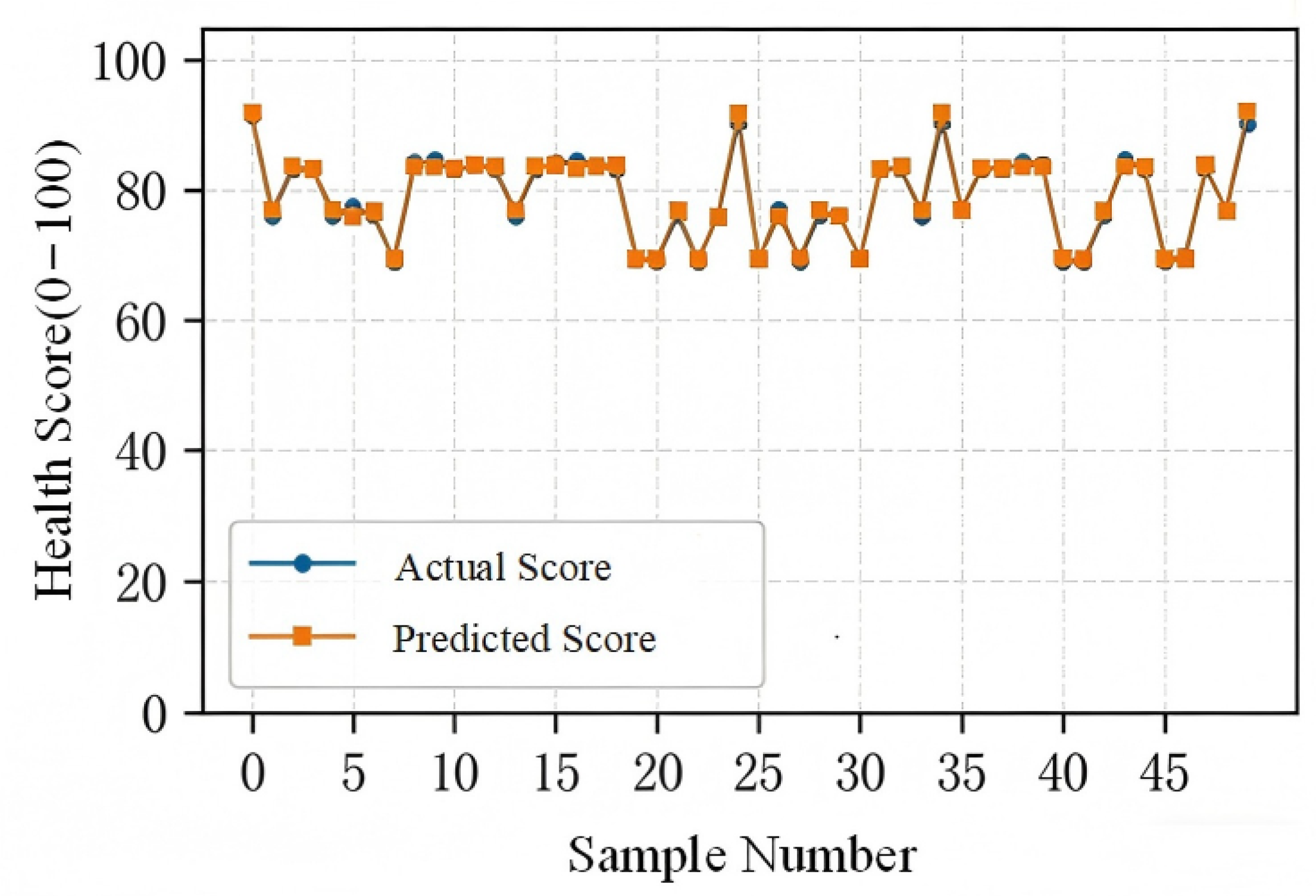
where $H{S}_t^{final}$ represents the final comprehensive health score at time t, and $\lambda \in [0, 1]$ is the weighting coefficient used to balance the current degradation assessment and the historical trend assessment. Compared with the time index, fault severity can more directly reflect the current damage state of the equipment [41]. Therefore, in this paper, damage severity is adopted as the dominant factor in health assessment with a weight of 0.95, while the time index is employed only to supplement the description of the degradation evolution trend with a weight of 0.05. This weighting scheme embodies the health assessment principle of a severity-dominant and time-trend-assisted health assessment principle [42]. Because independent health-score labels are unavailable in the CWRU dataset, the reported health scores should be regarded as derived reference scores based on severity labels and temporal indices. As shown in Figure 6, the differences between the actual and predicted scores for selected samples fell within 0–0.8 health-score points.

Figure 6. Comparison between derived reference scores and model-derived scores.

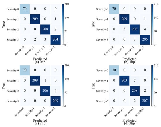
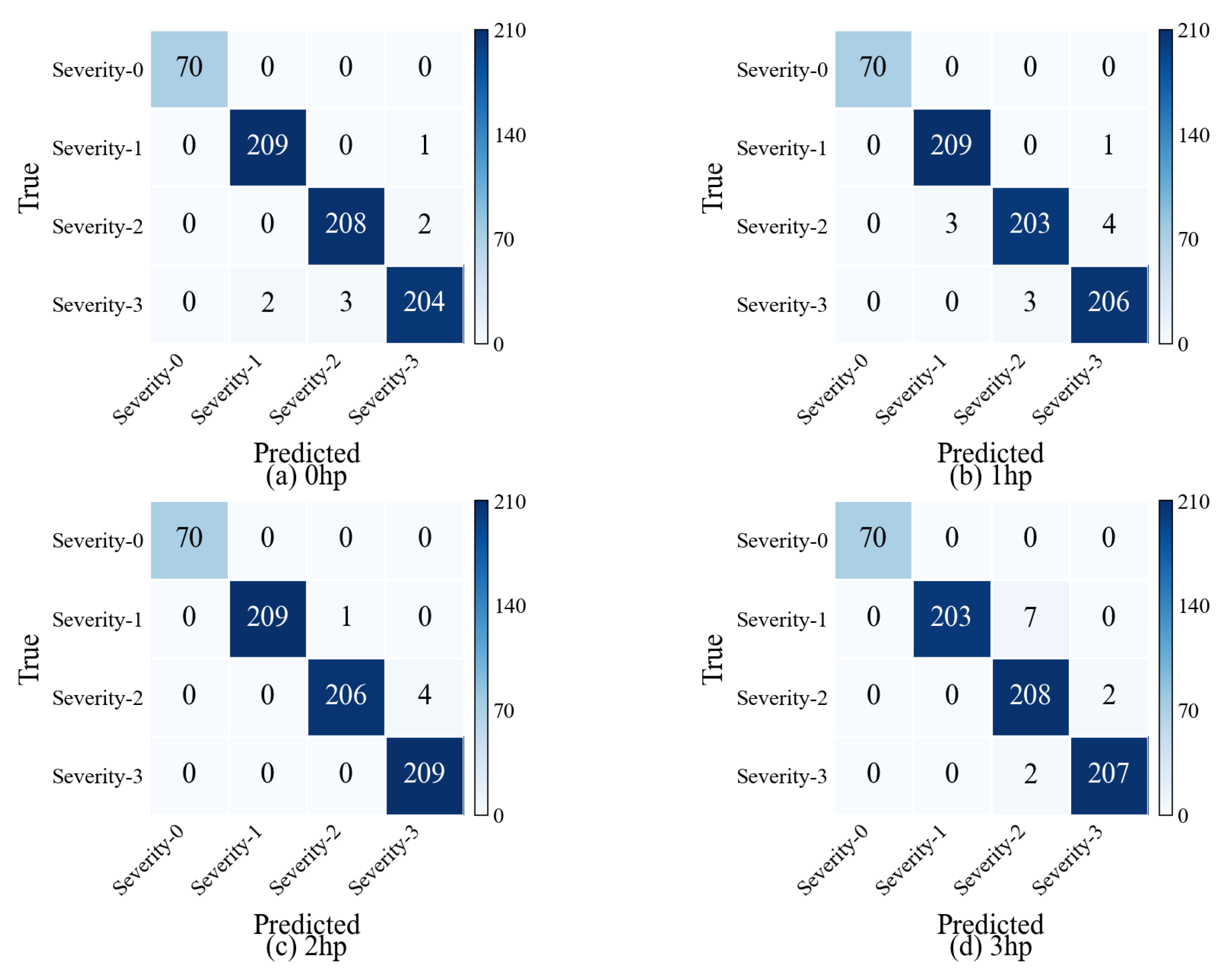
For the joint prediction of bearing fault type and fault severity under different load conditions, samples collected under the four load levels are used for mixed training and validation. The confusion matrices for fault severity prediction are shown in Figure 7. The results show that normal samples are correctly classified under all four load conditions, indicating that the model can reliably distinguish healthy states from faulty states. For faulty samples, only a small number of misclassifications are observed. These errors mainly occur between adjacent severity levels, such as Severity-2 and Severity-3, suggesting that fault severities with similar vibration characteristics are more difficult to distinguish. Despite these minor misclassifications, the proposed model maintains high overall severity prediction performance, achieving an average accuracy of 98.99% across repeated experiments under different load conditions.

Figure 7. Fault severity prediction under different load conditions.

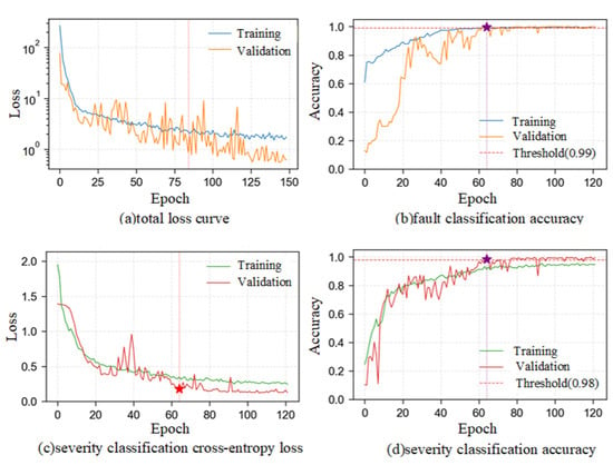
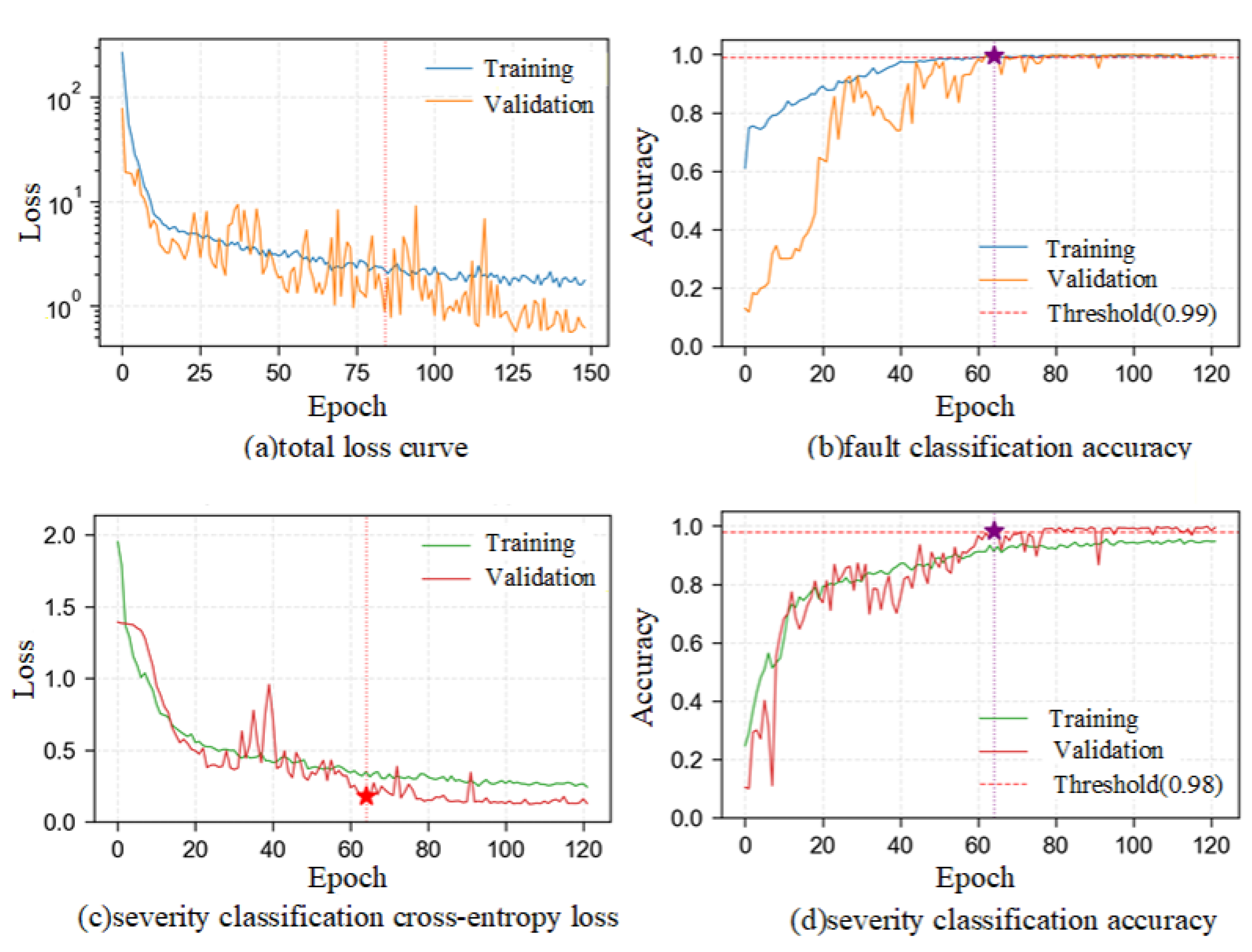
The corresponding training curves are shown in Figure 8, including the total loss, fault classification accuracy, severity classification loss, and severity classification accuracy. Both the training and validation losses decrease rapidly in the early training stage and then gradually stabilize, indicating that the model converges effectively during mixed-load training. Meanwhile, the training and validation accuracies increase steadily and remain close to each other after convergence. This suggests that no obvious overfitting occurs and that the model can learn fault-related features from mixed-load vibration signals. Overall, the results demonstrate that the proposed framework achieves stable performance in both fault diagnosis and severity prediction under different load conditions.

Figure 8. Training and validation curves for fault classification and severity prediction under different loads (The vertical dashed lines and star markers in the figure represent the model parameters saved upon first reaching the standard).

3.4. Validation of Anti-Noise Performance

In practical industrial environments, the collected bearing vibration signals are often contaminated by noise of varying intensities due to friction among mechanical components, equipment vibration, and external environmental interference, which severely degrades the accuracy of bearing fault diagnosis [43]. To evaluate the anti-noise capability of the proposed model, Gaussian white noise with different intensities is added to the sample datasets under different load conditions to simulate actual signal acquisition under noisy operating conditions. The intensity of the injected noise is quantified by the signal-to-noise ratio (SNR), which is defined as follows:

$$SNR=10\times log{\displaystyle \frac{P_s}{P_n}}$$

(19)

where $P_s$ and $P_n$ represent the power or intensity of the original pure signal and the added Gaussian white noise, respectively.

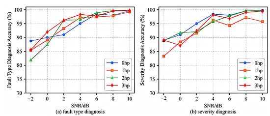
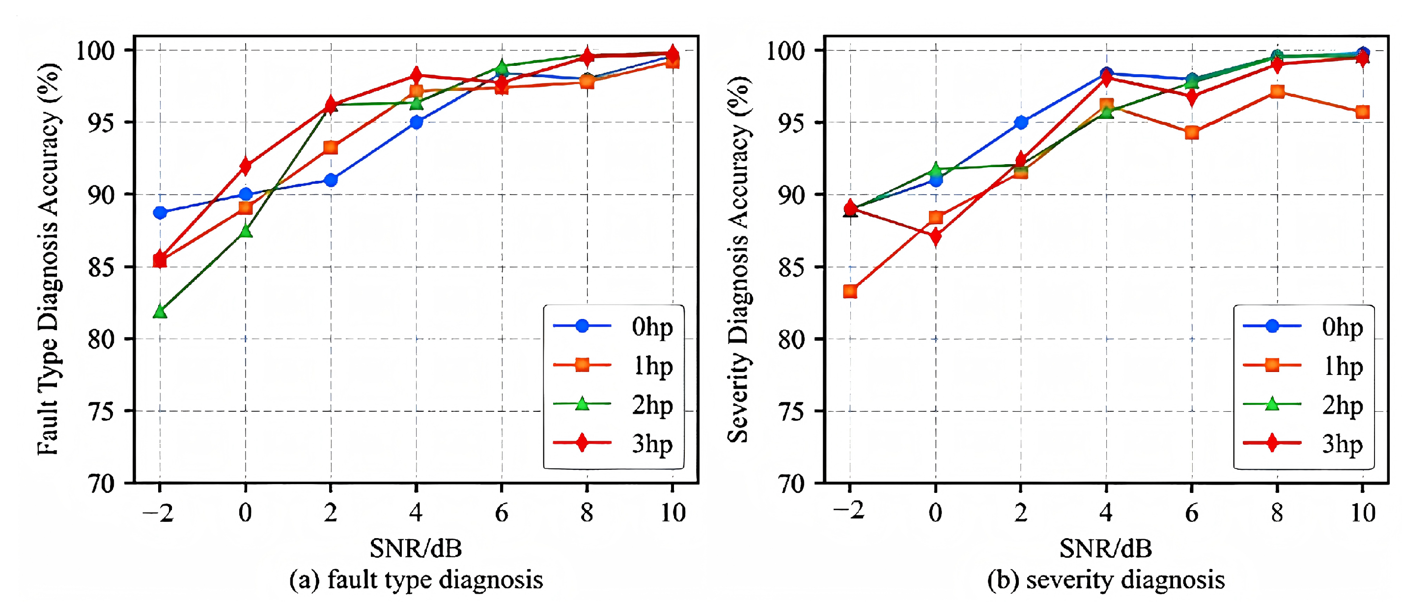
In the experiments, Gaussian white noise with SNR values ranging from −2 dB to 10 dB is added to the sample datasets under different load conditions, and the fault diagnosis accuracy and fault severity prediction accuracy of the proposed model are evaluated. The results are shown in Figure 9. Under different load conditions, both accuracies generally increased as the SNR increased. When the SNR was higher than 4 dB, both accuracies approached 95%, while the model still achieved accuracies above 80% at an SNR of −2 dB.

Figure 9. Average prediction accuracy of different loads versus SNR.

This performance can be attributed to the PPCA-based global denoising and EMD-based effective component reconstruction performed during preprocessing, which help suppress noise interference and retain useful fault-related components. These results indicate that the proposed model has improved tolerance to simulated Gaussian white noise under the tested SNR conditions.

3.5. Ablation Analysis of PPCA-EMD Preprocessing and Network Modules

To further verify the contributions of the PPCA-EMD preprocessing strategy and the key neural network modules, ablation experiments are conducted for each module while keeping all model training parameters consistent. It should be noted that, to evaluate the preprocessing effectiveness of PPCA and EMD on the original signals, the raw signals used in the ablation experiments are contaminated with Gaussian white noise at an SNR of 2 dB. To assess the influence of different modules on model performance, nine ablation variants are constructed using the complete model as the baseline. Model A represents the complete model containing all modules. Models B, C, E, F, and G remove the PPCA, EMD, 1DCNN, BiGRU, and attention modules, respectively. In addition, to further verify the role of the overall preprocessing module and combined neural network components, models without the PPCA-EMD, BiGRU-Attention, and 1DCNN-Attention modules are constructed and denoted as Models D, H, and I, respectively. The accuracy, precision, F1-score, and recall of the complete model and its ablation variants on the test set are reported in Table 7.

Table 7. Comparison of ablation study results.

Model Name	Accuracy (%)	Precision (%)	F1-Score (%)	Recall (%)
Model A	96.31 ± 2.58	96.20	96.19	96.18
Model B	92.06 ± 3.26	91.76	92.34	90.87
Model C	93.37 ± 4.61	92.37	93.35	92.41
Model D	90.49 ± 6.64	91.05	90.32	90.15
Model E	63.95 ± 3.88	73.07	66.92	64.74
Model F	91.27 ± 2.36	92.99	92.24	92.04
Model G	93.57 ± 0.34	93.77	93.55	93.55
Model H	79.71 ± 0.19	78.45	78.71	79.57
Model I	61.55 ± 4.23	64.57	62.31	63.38

Under the 2 dB noise condition, the results of the ablation experiments are shown in Table 7. The complete model achieved the highest fault diagnosis accuracy of 96.31%. When PPCA denoising is removed and only EMD-based reconstruction is retained, the accuracy decreases to 93.37%, indicating that PPCA contributes to noise suppression and improves the stability of the reconstructed signals. When EMD is removed and only PPCA-denoised signals are used, the accuracy further decreases to 92.06%, suggesting that EMD-based decomposition and IMF reconstruction are important for retaining fault-related components under noisy conditions. The raw signal input without PPCA-EMD preprocessing achieved an accuracy of 90.49% and exhibited the largest performance fluctuation. Compared with the raw signal input, the complete PPCA-EMD strategy improved the accuracy by 5.82 percentage points and reduced the standard deviation from 6.64% to 2.58%. These results indicate that PPCA and EMD play complementary roles: PPCA suppresses background noise, whereas EMD enhances the reconstruction of fault-related signals. Therefore, the combined PPCA-EMD preprocessing strategy provides a more noise-tolerant input representation under the tested low-SNR condition. After removing the attention mechanism, the accuracy decreases to 93.57%, a reduction of 2.74 percentage points, indicating that the attention module improves discriminative feature weighting and enhances classification performance. When the BiGRU module is removed, the accuracy decreases to 91.27%, suggesting that bidirectional temporal dependency modeling is important for capturing sequential fault-related patterns. The 1DCNN-only model achieved an accuracy of 79.71%, indicating that convolutional local feature extraction alone is insufficient to fully represent temporal fault characteristics. In contrast, removing the 1DCNN module caused a substantial accuracy drop to 63.95%, while the BiGRU-only configuration achieved only 61.55%. These results demonstrate that the 1DCNN module provides a fundamental contribution by extracting local fault features from vibration signals, whereas the BiGRU and attention modules further improve performance through temporal modeling and adaptive feature enhancement. Overall, the superior performance of the proposed model is attributed to the complementary integration of convolution-based local feature extraction, bidirectional temporal sequence learning, and attention-based feature weighting.

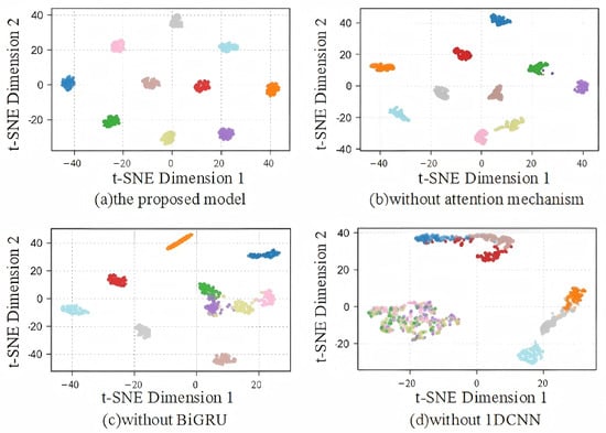
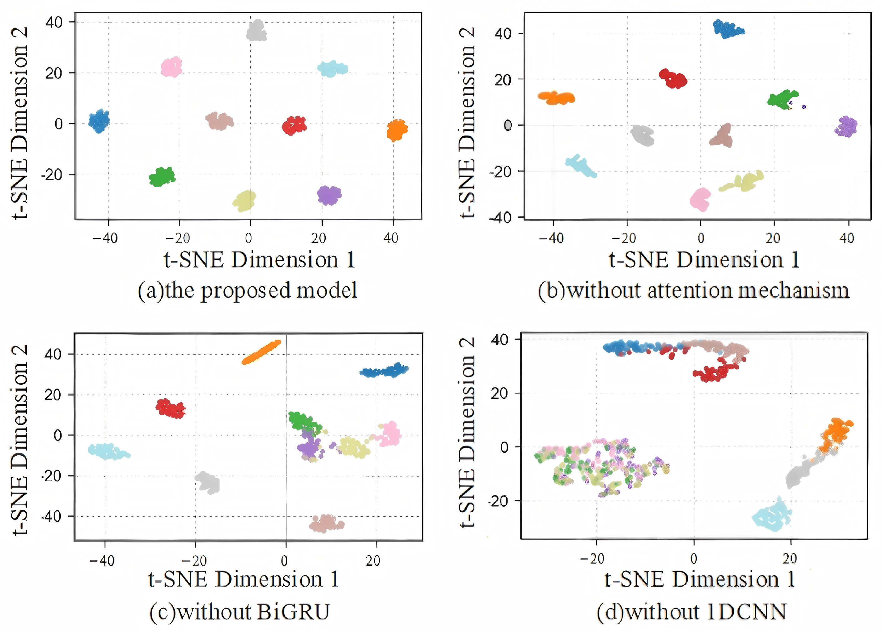
To further illustrate the influence of each module on feature representation, t-distributed stochastic neighbor embedding (t-SNE) is employed to visualize the high-dimensional features learned by different model configurations. The corresponding feature distributions are shown in Figure 10.

Figure 10. Visualization of feature distributions using t-SNE for different ablation configurations.

The complete proposed model produces more compact and better-separated feature clusters than the ablated models. In contrast, the feature distributions of the ablated models exhibit different degrees of overlap and dispersion. In particular, removing the 1DCNN module leads to the most obvious feature mixing, indicating that convolutional local feature extraction plays an important role in distinguishing fault categories. Removing the BiGRU module also increases the overlap between some classes, suggesting that temporal modeling contributes to the separation of fault-related features. In addition, the model without the attention mechanism still forms distinguishable clusters, but its feature compactness and inter-class separation are weaker than those of the complete model. The t-SNE visualization results are consistent with the quantitative ablation results. These findings suggest that the performance of the proposed model benefits from the complementary integration of convolutional local feature extraction, bidirectional temporal modeling, and attention-based feature weighting.

3.6. Cross-Load Validation on Public Datasets and Supplementary Industrial Case Study

To evaluate the limited-sample transfer capability of the proposed framework under operating-condition shifts, cross-load experiments are conducted on the CWRU and PU datasets, followed by a supplementary cross-unit production-line case study. Four transfer strategies are compared, including direct transfer, hard pseudo-label-based fine-tuning of the classification head, fine-tuning of the classification head with target-domain labels, and partial-layer freezing under hard pseudo labels. In the partial-freezing strategy, the first two 1DCNN layers are frozen, whereas the subsequent 1DCNN layer, BiGRU layers, self-attention module, shared dense layer, and task-specific output branches are kept trainable. This design aims to preserve generic low-level vibration and impulse features learned from the source domain while allowing higher-level representations to adapt to the target operating condition [44].

3.6.1. Cross-Load Experiment Conducted on the CWRU Dataset

The corresponding results are summarized in Table 8. It should be noted that the accuracy of the proposed framework reported in this table is obtained under the direct-transfer setting. As shown in Table 8, the proposed method achieves the highest mean accuracy of 87.24%, outperforming 1DCNN-Transformer, WDCNN, and ECTN by 7.71, 10.21, and 3.45 percentage points, respectively. In the single-source transfer tasks, the proposed method obtains the best results in the 1 → 2 hp and 2 → 1 hp tasks, with accuracies of 90.31% and 83.93%, respectively, while maintaining competitive performance in the 2 → 3 hp and 3 → 2 hp tasks. In the multi-source transfer tasks, the proposed method achieves 93.25% for 1 + 2 → 3 hp and 95.78% for 1 + 3 → 2 hp, both higher than the comparison models. These results indicate that the proposed framework can effectively extract transferable fault features and maintain improved cross-load diagnostic performance in the tested tasks.

Table 8. Comparison results of different models under different transfer tasks (%).

Transfer Task	1DCNN-Transformer	WDCNN	ECTN	The Proposed Method
1 → 2 hp	$78.24\pm 0.41$	$77.10\pm 3.34$	$83.53\pm 3.17$	$90.31\pm 1.76$
2 → 3 hp	$70.94\pm 1.15$	$73.67\pm 3.45$	$82.50\pm 2.80$	$81.34\pm 2.35$
2 → 1 hp	$80.04\pm 0.64$	$76.04\pm 1.34$	$73.84\pm 4.39$	$83.93\pm 0.67$
3 → 2 hp	$79.93\pm 0.20$	$70.77\pm 1.42$	$81.46\pm 2.36$	$78.60\pm 0.39$
1 + 2 → 3 hp	$83.76\pm 4.01$	$76.39\pm 5.97$	$87.49\pm 3.92$	$93.25\pm 1.40$
1 + 3 → 2 hp	$87.53\pm 3.88$	$88.22\pm 1.81$	$93.91\pm 0.33$	$95.78\pm 0.67$
Mean	$80.07$	$77.03$	$83.79$	$87.24$

Table 9 presents the average accuracy of different strategies under the conditions of n = 10, n = 30, and n = 50, respectively, where n represents the number of randomly sampled target-domain instances. Compared with direct transfer, the partial-freezing strategy achieves higher accuracy under all tested sample settings, indicating that updating only the higher-level and task-related layers can help the model adapt to the target load condition while retaining useful source-domain representations. Although labeled-head fine-tuning achieves the highest accuracy in some settings when labeled target samples are available, its performance relies on target-domain annotations. By contrast, the partial-freezing strategy provides a lightweight adaptation mechanism that reduces the need to update all parameters and preserves the transferable shallow features learned from the source domain. These results suggest that partial freezing is a reasonable and stable cross-load adaptation strategy under limited-sample conditions, especially when target-domain annotations are insufficient or costly to obtain.

Table 9. Accuracy comparison of different transfer strategies under 1 + 3 hp → 2 hp (%).

Transfer Task/Shot	n = 10	n = 30	n = 50
Exp 1: Direct Transfer	$95.78\pm 0.67$
Exp 2: Unlabeled Head	$96.60\pm 0.74$	$96.98\pm 1.37$	$97.24\pm 0.88$
Exp 3: Labeled Head	$96.77\pm 0.96$	$98.35\pm 0.82$	$98.66\pm 0.35$
Exp 4: Partial Frozen	$96.55\pm 0.79$	$97.64\pm 0.84$	$97.05\pm 1.67$

The accuracy of Exp1 is independent of the value of n.

3.6.2. Cross-Load Experiment Conducted on the PU Dataset

The PU cross-load experiment provides additional evidence under a dataset containing more realistic bearing damage. As shown in Table 10, direct transfer achieves a relatively high accuracy, suggesting that the proposed framework can learn source-domain representations with a certain degree of cross-load generalization. Nevertheless, the strategies involving target-domain adaptation generally lead to further improvements, indicating that distributional discrepancies between N15M07 and N15M01 still affect the direct generalization of the pretrained model.

Table 10. Accuracy comparison of different limited-sample transfer strategies on the PU dataset under the N15M07 → N15M01 condition (%).

Transfer Task	n = 10	n = 30	n = 50
Exp 1: Source Domain Accuracy	$99.52\pm 0.12$
Exp 2: Direct Transfer	$96.08\pm 1.27$
Exp 3: Unlabeled Head	$97.13\pm 1.23$	$96.71\pm 1.56$	$96.60\pm 1.78$
Exp 4: Labeled Head	$97.29\pm 0.79$	$97.38\pm 0.71$	$97.27\pm 1.02$
Exp 5: Partial Frozen	$97.18\pm 0.71$	$97.55\pm 0.77$	$96.99\pm 1.19$

The accuracies of Exp1 and Exp2 are independent of the value of n. Exp denotes experiment.

Among the evaluated strategies, the partial-freezing strategy maintains competitive and stable performance across different target-sample sizes. This result supports the layer-wise design of the proposed transfer scheme. The frozen shallow 1DCNN layers preserve generic local vibration patterns and impulse-related features that are likely to remain informative across different torque conditions. Meanwhile, the unfrozen deeper 1DCNN layer, the BiGRU layers and the self-attention module, shared dense layer, and task-specific branches allow the model to adjust temporal representations and decision boundaries according to the target operating condition. In this way, partial freezing reduces unnecessary modification of transferable low-level features while maintaining sufficient flexibility for target-domain adaptation. Compared with direct transfer, the partial-freezing strategy alleviates the degradation caused by operating-condition shifts. Compared with head-only fine-tuning, it adapts not only the final decision layer but also the higher-level temporal and attention-based representations, which is beneficial when the source and target domains differ in load-dependent signal characteristics. Therefore, the PU results further support the effectiveness of partial freezing as a limited-sample cross-load transfer strategy.

3.6.3. Cross-Unit Production-Line Case Study

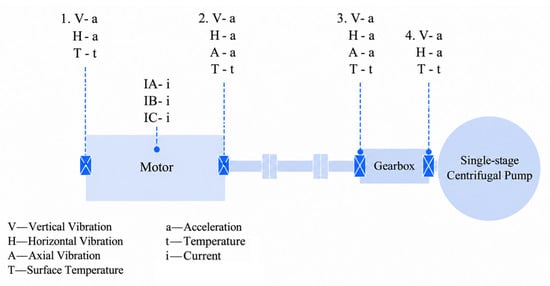
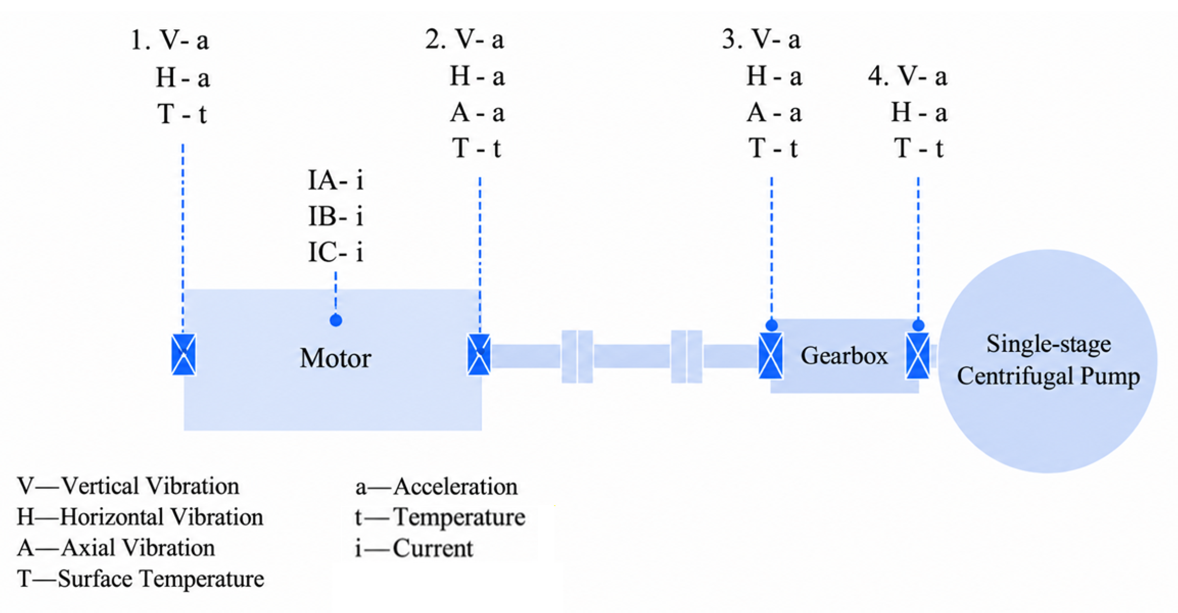
A production-line case study is additionally included to illustrate the preliminary feasibility of applying the proposed workflow to real monitoring signals. The sampling frequency is 12 kHz and the operating speed of the pump unit is 2981 r/min. The schematic diagram of the unit structure is shown in Figure 11.

Figure 11. Schematic diagram of P-2101A/B high-temperature condensate pump.

The data are collected from the drive-end bearing position of the P-2101B and P-2101A units. Specifically, 300 samples for each of the four fault types are collected from the P-2101A unit, and 100 samples from the P-2101B unit. The four bearing conditions correspond to normal operation, poor lubrication, overload and component fit loosening. All equipment condition data are verified through maintenance reports. A cross-unit training strategy is then adopted, in which the model is trained on the P-2101A dataset and evaluated on the P-2101B dataset. Table 11 presents the accuracy comparison results of cross-unit experiments.

Table 11. Accuracy comparison of cross-unit experiments under the P-2101A → P-2101B condition (%).

Transfer Task	n = 10	n = 30	n = 50
Exp 1: Source Domain Accuracy	$100.00\pm 0.00$
Exp 2: Direct Transfer	$54.95\pm 2.80$
Exp 3: Unlabeled Head	$68.06\pm 1.52$	$69.78\pm 2.40$	$70.00\pm 2.84$
Exp 4: Labeled Head	$85.05\pm 8.58$	$91.29\pm 2.56$	$91.51\pm 2.24$
Exp 5: Partial Frozen	$92.47\pm 2.43$	$93.98\pm 1.04$	$93.12\pm 5.81$

The accuracies of Exp1 and Exp2 are independent of the value of n.

As shown in Table 11, among the compared strategies, the partial-freezing strategy achieved the best overall performance, with accuracies of 92.47%, 93.98%, and 93.12% under n = 10, n = 30, and n = 50, respectively. Relative to direct transfer, the corresponding improvements were 37.52, 39.03, and 38.17 percentage points. Compared with unlabeled-head fine-tuning and labeled-head fine-tuning, partial freezing also achieved consistent gains. These results indicate that partial freezing provides a better balance between source-domain feature reuse and target-unit adaptation. By freezing the shallow 1DCNN layers, generic vibration waveforms and impulse-related features learned from the P-2101A unit can be retained, while the higher-level convolutional, temporal, attention-based, and task-specific layers remain trainable to adapt to the P-2101B unit. Therefore, the proposed partial-freezing strategy can reduce the performance degradation caused by direct cross-unit transfer under limited target-domain samples. Nevertheless, because the production-line dataset is limited in scale, these results should be interpreted as preliminary evidence of cross-unit application feasibility rather than conclusive proof of broad industrial generalization.

4. Conclusions

In this study, a preprocessing-assisted multitask framework for rolling bearing fault diagnosis and severity prediction is developed by integrating PPCA-EMD signal reconstruction with a 1DCNN-BiGRU-Attention network. By integrating PPCA denoising with EMD-based signal decomposition and reconstruction, the proposed preprocessing strategy effectively suppresses noise interference while preserving fault-relevant information in raw vibration signals. The 1DCNN-BiGRU architecture further enables joint fault classification and severity prediction through shared feature learning, thereby improving feature sharing and model efficiency. Experimental results on the CWRU dataset demonstrate that the proposed method achieves an average fault diagnosis accuracy of 99.71% and an average severity prediction accuracy of 98.99%. Moreover, the cross-load experiments conducted on the CWRU and PU datasets provide preliminary evidence of the adaptability of the proposed framework under varying operating conditions and suggest the effectiveness of the partial-layer freezing transfer strategy. The production-line case serves as a supplementary preliminary feasibility study for cross-equipment transfer.

However, this study still has several limitations. Owing to the limited number of fault samples obtained from the actual production line, the current industrial validation is restricted to a small number of samples, fault types, and specific operating conditions. Therefore, when the proposed method is applied to other equipment types or different operating environments, domain discrepancies may lead to performance degradation. Improving cross-equipment and cross-scenario adaptability through domain adaptation and transfer learning techniques remains an important direction for future research. Future work will focus on enhancing the interpretability, adaptability, and deployment efficiency of the proposed framework. Specifically, attention-weight analysis and post hoc interpretability methods will be explored to better understand the learned fault-related features.

References

- Xu, S.; Zhang, W.; Pang, S.; Wu, S.; Zhao, R.; Qin, Y.; Guo, P. A rolling bearing fault diagnosis method based on the STRN-CM model. Machines 2026, 14, 279. [Google Scholar] [CrossRef] [Scilit]
- Bai, X.; Zhong, X.; Liu, Y.; Zhang, K.; Meng, W.; Li, J.; Zhang, X. Fault diagnosis of rolling bearings based on an ascending-dimension convolutional neural network. Machines 2026, 14, 302. [Google Scholar] [CrossRef] [Scilit]
- Qiu, W.; Wang, B.; Hu, X. Rolling bearing fault diagnosis based on RQA with STD and WOA-SVM. Heliyon 2024, 10, e26141. [Google Scholar] [CrossRef] [Scilit] [PubMed]
- Wei, J.N.; Huang, H.S.; Yao, L.G.; Hu, Y.; Fan, Q.S.; Huang, D. New imbalanced fault diagnosis framework based on Cluster-MWMOTE and MFO-optimized LS-SVM using limited and complex bearing data. Eng. Appl. Artif. Intell. 2020, 96, 103966. [Google Scholar] [CrossRef] [Scilit]
- Shao, X.; Li, D.; Ra, I.; Kim, C. DSMT-1DCNN: Densely supervised multitask 1DCNN for fault diagnosis. Knowl.-Based Syst. 2024, 292, 111609. [Google Scholar] [CrossRef] [Scilit]
- Talukder, R.; Siddique, F.; Rana, S. Regression (REG-1DCNN)-based unsupervised bridge damage detection using vehicle-induced acceleration response and dynamic time warping algorithm. Measurement 2025, 256, 118380. [Google Scholar] [CrossRef] [Scilit]
- Wu, L.; Ding, N.; Wang, L.; Li, J.; Zhang, H. Physics-informed attention LSTM: A dual-knowledge fusion framework for interpretable bearing fault diagnosis under small-data scenarios. Measurement 2026, 263, 120216. [Google Scholar] [CrossRef] [Scilit]
- Wu, C.; Cai, H.; Huang, W.; Yang, M. An OFSCoh-M-SSAE intelligent fault diagnosis method for rotating machinery under time-varying speed conditions. Meas. Sci. Technol. 2026, 37, 126114. [Google Scholar] [CrossRef] [Scilit]
- Gao, S.; Li, T.; Zhang, Y.; Pei, Z. Fault diagnosis method of rolling bearings based on adaptive modified CEEMD and 1DCNN model. ISA Trans. 2023, 140, 309–330. [Google Scholar] [CrossRef] [Scilit] [PubMed]
- Ma, S.; Shi, S.; Zhang, Y.; Gao, H. A high-precision method for detecting rolling bearing faults in unmanned aerial vehicle based on improved 1DCNN-Informer model. Measurement 2025, 256, 118200. [Google Scholar] [CrossRef] [Scilit]
- Xia, L.; Wang, D.; Chen, C.; Xie, C.; Deng, J. Bearing fault diagnosis method based on IMSE-CNN-Transformer and immune genetic algorithm optimization. Appl. Soft Comput. 2026, 194, 114918. [Google Scholar] [CrossRef] [Scilit]
- Liu, P.J.; Lv, H.Z.; Wang, L.J.; Yang, X.C.; He, Z.K.; Zhang, R.S. Experimental Cross-Domain Bearing Fault Diagnosis Method Based on Local Mean Decomposition and Improved Transfer Component Analysis. Machines 2026, 14, 216. [Google Scholar] [CrossRef] [Scilit]
- Zhang, D.; Hao, Y.; Li, H.; Gong, C.; He, J.; Fei, Q. Time-frequency convolutional-Transformer network with attention fusion for rotor system fault diagnosis. Meas. Sci. Technol. 2026, 37, 126101. [Google Scholar] [CrossRef] [Scilit]
- Zhang, S.; Song, B.; Zhao, F.; Sun, G.; Meng, F. A decoupling method for compound faults of rolling bearings based on multi-modal bidirectional cross-attention fusion and contrastive learning. Meas. Sci. Technol. 2025, 36, 106131. [Google Scholar] [CrossRef] [Scilit]
- Yang, J.; Han, H.; Dong, X.; Wang, G.; Zhang, S. Bearing Fault Diagnosis Grounded in the Multi-Modal Fusion and Attention Mechanism. Appl. Sci. 2025, 15, 1531. [Google Scholar] [CrossRef] [Scilit]
- Xu, J.; Zhang, L.; Chen, J.; Zhang, H.; Liang, L. A multilevel feature extraction framework based on FMD-CWT and HP-ResNet for bearing fault diagnosis. Measurement 2026, 257, 118903. [Google Scholar] [CrossRef] [Scilit]
- Wu, M.; Yao, Z.; Verbeke, M.; Karsmakers, P.; Gorissen, B.; Reynaerts, D. Data-driven models with physical interpretability for real-time cavity profile prediction in electrochemical machining processes. Eng. Appl. Artif. Intell. 2025, 160, 111807. [Google Scholar] [CrossRef] [Scilit]
- Bai, X.; Wang, Y.; Zhang, C. Research on denoising of rolling bearing vibration signals based on the ISSA-VMD-JWTD method. Digit. Signal Process. 2026, 173, 105912. [Google Scholar] [CrossRef] [Scilit]
- Yong, W.; Li, Y.; Yu, L.; Zhang, X. A novel denoising method for bearing vibration signals in rotating machinery based on CEEMDAN-PSO-TV combined AWR and DRC. Measurement 2026, 268, 120641. [Google Scholar] [CrossRef] [Scilit]
- Shen, J.; Wang, Z.; Wang, Y.; Zhu, H.; Zhang, L.; Tang, Y. AGWO-PSO-VMD-TEFCG-AlexNet bearing fault diagnosis method under strong noise. Measurement 2025, 242, 116259. [Google Scholar] [CrossRef] [Scilit]
- Li, H.; Liu, T.; Wu, X.; Chen, Q. An optimized VMD method and its applications in bearing fault diagnosis. Measurement 2020, 166, 108185. [Google Scholar] [CrossRef] [Scilit]
- Xiang, J.; Zhong, Y.; Gao, H. Rolling element bearing fault detection using PPCA and spectral kurtosis. Measurement 2015, 75, 180–191. [Google Scholar] [CrossRef] [Scilit]
- Nodehi, A.; Golalizadeh, M.; Maadooliat, M.; Agostinelli, C. Torus probabilistic principal component analysis. J. Classif. 2025, 42, 1–22. [Google Scholar] [CrossRef] [Scilit]
- Shi, P.; An, S.; Li, P.; Han, D. Signal feature extraction based on cascaded multi-stable stochastic resonance denoising and EMD method. Measurement 2016, 90, 318–328. [Google Scholar] [CrossRef] [Scilit]
- Chen, Y.; Yulin, W.; Guocai, M.; Yan, W.; Yuxin, S.; Yan, H. Weak fault feature extraction of rolling bearings based on improved ensemble noise-reconstructed EMD and adaptive threshold denoising. Mech. Syst. Signal Process. 2022, 171, 108834. [Google Scholar] [CrossRef] [Scilit]
- Wan, A.; Li, P.; Bukhaiti, A.K.; Cheng, X.; Ji, X.; Wang, J.; Shan, T. Fault diagnosis of air conditioning compressor bearings using wavelet packet decomposition and improved 1DCNN. Next Energy 2025, 9, 100424. [Google Scholar] [CrossRef] [Scilit]
- Wang, M.; Wang, Z. A novel CNN-transformer integrated with cross-attention mechanism for intelligent diagnosis of rolling bearing faults. Digit. Signal Process. 2026, 175, 105996. [Google Scholar] [CrossRef] [Scilit]
- Wang, X.; Mao, D.; Li, X. Bearing fault diagnosis based on vibro-acoustic data fusion and 1D-CNN network. Measurement 2021, 173, 108518. [Google Scholar] [CrossRef] [Scilit]
- Zhang, Z.; Zhang, J.; Zhao, H.; Zhang, S.; Yang, X.; Wang, Y. Short-term wind power prediction based on GWO-VMD-FE and TCN-BiGRU. Electr. Power Syst. Res. 2026, 253, 112568. [Google Scholar] [CrossRef] [Scilit]
- Ahmad, H.S.; Kai, H.J.; Rabiu, I.B.; Hassan, S.M.H.U. Fault diagnosis of aircraft engine using an ANN-BiGRU based on perturbation strategy. Aerosp. Sci. Technol. 2026, 168, 111047. [Google Scholar] [CrossRef] [Scilit]
- Deng, L.; Zhao, C.; Yan, X.; Zhang, Y.; Qiu, R. A novel approach for bearing fault diagnosis in complex environments using PSO-CWT and SA-FPN. Measurement 2025, 249, 117027. [Google Scholar] [CrossRef] [Scilit]
- Wu, Y.; Chen, Z.; Wu, L.; Lin, P.; Cheng, S.; Lu, P. An intelligent fault diagnosis approach for PV array based on SA-RBF kernel extreme learning machine. Energy Procedia 2017, 105, 1070–1076. [Google Scholar] [CrossRef] [Scilit]
- Cao, X.; Zhang, Q.; Liu, Q.; Li, J. ARAM-Swin: A hybrid architecture with an adaptive residual attention module and Swin Transformer for rolling bearing fault diagnosis. Meas. Sci. Technol. 2026, 37, 126112. [Google Scholar] [CrossRef] [Scilit]
- Liu, Z.; Wang, H.; Liu, J.; Qin, Y.; Peng, D. Multitask Learning Based on Lightweight 1DCNN for Fault Diagnosis of Wheelset Bearings. In IEEE Transactions on Instrumentation and Measurement; IEEE: New York, NY, USA, 2021; Volume 70, pp. 1–11. [Google Scholar] [CrossRef] [Scilit]
- Liu, S.; Wu, Z.; Gao, J.; Sun, W.; Yuan, Y.; Fan, L. Rolling bearing fault diagnosis method based on an improved 1DCNN-Transformer. Machines 2026, 14, 629. [Google Scholar] [CrossRef] [Scilit]
- Zhang, W.; Peng, G.; Li, C.; Chen, Y.; Zhang, Z. A new deep learning model for fault diagnosis with good anti-noise and domain adaptation ability on raw vibration signals. Sensors 2017, 17, 425. [Google Scholar] [CrossRef] [Scilit] [PubMed]
- Hao, S.; Ge, F.; Li, Y.; Jiang, J. Multisensor bearing fault diagnosis based on one-dimensional convolutional long short-term memory networks. Measurement 2020, 159, 107802. [Google Scholar] [CrossRef] [Scilit]
- Liu, W.; Zhang, Z.; Zhang, J.; Huang, H.; Zhang, G.; Peng, M. A novel fault diagnosis method of rolling bearings combining convolutional neural network and transformer. Electronics 2023, 12, 1838. [Google Scholar] [CrossRef] [Scilit]
- Chen, C.; Liu, L. Health assessment of rolling bearings based on multivariate state estimation and reliability analysis. Appl. Sci. 2025, 15, 5396. [Google Scholar] [CrossRef] [Scilit]
- Huang, G.; Wu, S.; Wang, Q.; Wei, W.; Fu, Y.; Wang, N.; Lei, L. Rolling bearing health indicator: From design to modeling and evaluation. Intell. Sustain. Manuf. 2025, 2, 10025. [Google Scholar] [CrossRef] [Scilit]
- Song, C.; Liu, K. Statistical degradation modeling and prognostics of multiple sensor signals via data fusion: A composite health index approach. IISE Trans. 2018, 50, 853–867. [Google Scholar] [CrossRef] [Scilit]
- Zhao, S.; Li, P.; Kang, Y.; Zhao, Y. A health indicator enabling both first predicting time detection and remaining useful life prediction: Application to rotating machinery. Measurement 2024, 235, 114994. [Google Scholar] [CrossRef] [Scilit]
- Cao, Z.; He, L.; Hou, J. A bearing fault diagnosis method based on Hopfield network stochastic resonance and a multi-feature fusion health index. Measurement 2026, 266, 120500. [Google Scholar] [CrossRef] [Scilit]
- Djaballah, S.; Meftah, K.; Khelil, K.; Sayadi, M. Deep transfer learning for bearing fault diagnosis using CWT time-frequency images and convolutional neural networks. J. Fail. Anal. Prev. 2023, 23, 1046–1058. [Google Scholar] [CrossRef] [Scilit]
Disclaimer/Publisher’s Note: The statements, opinions and data contained in all publications are solely those of the individual author(s) and contributor(s) and not of MDPI and/or the editor(s). MDPI and/or the editor(s) disclaim responsibility for any injury to people or property resulting from any ideas, methods, instructions or products referred to in the content. |
© 2026 by the authors. Licensee MDPI, Basel, Switzerland. This article is an open access article distributed under the terms and conditions of the Creative Commons Attribution (CC BY) license.