Robust Fault-Tolerant Iterative Learning Control for Spatially Interconnected Systems in the Frequency Domain

Abstract

This study developed a frequency-domain fault-tolerant iterative learning control (ILC) strategy for spatially interconnected systems subject to external disturbances and actuator faults. An equivalent one-dimensional system model was established by performing model transformation and reformulation on the original spatially interconnected system. On this basis, the iterative learning control law was designed using two-dimensional system theory, and the closed-loop system was further characterized as an iterative process model. By applying the generalized Kalman–Yakubovich–Popov (KYP) lemma, it was demonstrated that within a finite frequency range, the resulting discrete repetitive process can guarantee both batch-wise stability and monotonic asymptotic convergence of the tracking error. Experimental results obtained from a precision collaborative machining platform verify the effectiveness of the proposed control method.

1. Introduction

A spatially interconnected system consists of many structurally similar subsystems interacting and coupling with each other spatially, where each subsystem may be a simple model that is easy to handle, but the whole system exhibits more complex behavioral characteristics that differ from those of the individual subsystems [1]. The most important characteristic of this type of system is that the information transfer between subsystems is a bidirectional coupling in the form of an interconnection chain, where each subsystem receives transmitted information from neighboring subsystems [2]. Due to the special structure of a spatially interconnected system, it is difficult to achieve efficient management and control of such systems using traditional centralized control when analyzing and controlling the system. Therefore, optimization of the control method by using the correlation between subsystems is informative for the study of this type of system.

Recently, spatial interconnection systems have been widely used in practical production such as aviation systems [3], smart grid systems [4], and networked intelligent body systems [5], and their trajectory tracking performance has become a hotspot for research. However, due to the coupling between the elements within the spatially interconnected system, its structure is often complex, and there is uncertainty in the structural model or parameters. In addition, actuator failures and various perturbations often occur in practical engineering, and these problems may lead to system instability and affect performance [6]. How to realize accurate tracking and performance improvement of spatially interconnected systems in complex environments is an important problem that needs to be solved.

In current practical engineering applications, limitations in the actuator operational range of physical systems often lead to situations where controller demands exceed actuator capabilities. When this occurs, the actuator cannot further increase its output, resulting in a deviation between the actual control signal and the desired value [7]. This deviation may lead to overshoots and oscillations in the response of the system, or even lead to complete destabilization of the system [8]. Several accidents caused by actuator failures have led scholars to gradually emphasize and investigate fault-tolerant control (FTC) [9]. The iterative learning FTC approach employs several key principles. First, it leverages the repetitive nature of ILC operations. Second, it incorporates prior knowledge from the learning process. The controller design maintains fixed structure and parameters throughout operation. This framework enables adjustment of FTC parameters during fault-control processes. These adjustments enhance system convergence performance. Additionally, they ensure the ILC process satisfies other specified performance requirements [10,11,12]. In practice, FTC can help the system to continue to operate when some components fail. Also fault diagnosis has significant potential in FTC [13,14].

In this research context, a wealth of results have been achieved for the FTC of different systems, both active and passive fault tolerance. The literature shows in detail the results of research in this field [15]. Specifically, for switching systems [16] and interconnected systems [17], research has focused on fault estimation and fault tolerance methods. For example, the literature proposes a distributed FTC method based on static output feedback, which utilizes the outputs of interconnected system for design and introduces a multi-constraint technique to enhance the suppression of external disturbances [18]. In terms of grid interconnection systems, a distributed fault estimation and FTC scheme with plug-and-play functionality was designed, a distributed fault estimation observer for each subsystem was built through a fully distributed approach, and a fault-compensated distributed FTC law based on the estimated states and faults was designed [19]. In addition, multiple parabolic partial differential equations were interconnected through a nonlinear coupling protocol, and a new method was developed using semi-Markovian switching laws to utilize the correlation information between the subsystems to enhance the fault-tolerance performance [20]. A new FE methodology was also developed to eliminate the effects of faults and disturbances through parametric design [21]. In nonlinear switching systems, for the problems of actuator failure and external perturbation, H∞ and a new fuzzy adaptive method were applied to optimize the gain respectively in order to improve the interval fault-tolerance accuracy [22,23].

Recent advances in fault-tolerant control have also been reported in diverse application domains. In the context of electric vehicles, FTC strategies have been developed to preserve vehicle stability and accommodate component failures with acceptable performance degradation [24]. For competitive neural networks subjected to deception attacks, actuator faults, and probabilistic time-varying delays, memory-based state feedback controllers combined with Lyapunov–Krasovskii functionals have been proposed to ensure robust state estimation [25]. For heterogeneous multiagent systems experiencing time-varying communication link faults and actuator faults, adaptive FTC schemes have been designed to compensate for channel signal fading and cyber bias attacks [26]. For discrete-time multiagent systems with sensor faults, data-driven observer-based fault detection methods and RBF neural network-based fault estimation approaches have been developed, followed by a distributed model-free sliding mode FTC law [27].

However, most of the existing algorithms are limited to fault detection and isolation in the time-domain analysis, failing to fully consider the relationship between interconnected systems and FTC from a frequency-domain perspective. Frequency-domain design methods are usually more suitable for the analysis and design of multivariable systems. These methods can effectively deal with the interactions and coupling effects between multiple input and output channels of a system, as well as the frequency-domain interactions [28]. As an example, an ILC dynamic adaptive matching method based on frequency domain adaptive Fourier decomposition is proposed for the dynamic characteristics of the system [29]. In addition, frequency-domain-based ILC methods, such as embedded frequency-domain ILC filters and basis functions, have been successfully applied to high-speed axis motion systems for industrial wire processing machines [30]. Furthermore, finite-frequency-domain designs have been shown to reduce conservatism compared with full-frequency designs [7]. However, these existing frequency-domain methods primarily focus on single systems or standard ILC frameworks. None of them simultaneously address spatially interconnected systems, actuator faults, and finite-frequency-domain ILC design. In contrast, the proposed method explicitly handles the spatial coupling between subsystems while operating in the finite frequency domain, achieving less conservative gains and faster fault recovery. Frequency-domain learning-based frequency selection methods have also been developed to remove trivial frequency components from the spectrum [31]. Addressing complex channel estimation challenges in MIMO systems, frequency-domain channel estimation strategies for compressed sensing have been explored [32].

In the current research frontier, the fault-tolerant method based on ILC has attracted much attention [33]. ILC utilizes the knowledge accumulated in previous iterations to achieve more precise tracking results [34,35]. Unlike conventional ILC methods that operate in the time domain or full-frequency domain, the proposed approach integrates fault-tolerant control with finite-frequency-domain ILC using the generalized KYP lemma. This integration ensures less conservative stability conditions and enables the controller to focus on the frequency range where the reference signal has dominant energy. As a control method that mimics the human learning process, ILC learns from historical information of completed batches to improve tracking performance within a fixed time interval [36]. ILC is especially suitable for systems with repetitive tasks and strict tracking requirements, such as hard disk tracking systems [37], gantry robot operating systems [38], wafer scanning photolithography systems [39], and distributed parameter systems [40].

Inspired by the above research, FTC of spatially interconnected systems with external disturbances and actuator faults is challenging. ILC has been shown to be an effective tool for solving fault diagnosis problems. Therefore, the development of a fast and fault-tolerant ILC-based approach for interconnected systems with external disturbances and actuator faults is of significant research value. To achieve this goal, an ILC-based control scheme was designed. The stability analysis and controller gain optimization were carried out in the finite frequency domain using the generalized KYP lemma, a fundamental frequency-domain tool. Within a finite frequency range that matches the spectral characteristics of the reference trajectory, stability conditions were derived, and the controller gains $K_1$, $K_2$, and $K_3$ were determined. Compared with traditional full-frequency methods, this finite-frequency-domain approach yields less conservative designs. The proposed control scheme is evaluated for spatially interconnected systems under actuator failure conditions to ensure satisfactory fault tolerance. In contrast to prior approaches [41], this work proposes a novel FTC strategy that rigorously guarantees system robustness and asymptotic stability under actuator fault conditions. The contributions of this paper are as follows:

1.

A reformulated modeling framework based on lifting transformation was constructed for spatially interconnected systems with multiple coupled subsystems. The two-dimensional spatial iteration dynamics were converted into an equivalent time-iteration domain model, which addresses bidirectional spatial coupling and differs from conventional modeling methods for single-system iterative learning control.

2.

Combined with the generalized KYP lemma, a finite-frequency domain fault-tolerant iterative learning control framework is presented for spatially interconnected systems. The derived stability constraints incorporate actuator fault parameters to guarantee stable iteration under fault and disturbance conditions and achieve less conservative designs compared with full-frequency schemes.

3.

This study presents a complete design and analysis procedure for applying finite-frequency methods to fault-tolerant iterative learning control of spatially interconnected systems. Verified by experimental tests, the obtained results can offer references for control design of similar interconnected systems.

2. Problem Description

This section first investigates the modeling of spatially interconnected systems. Initially, the original system is transformed into a two-dimensional system model related to both time and iteration steps by eliminating the interconnection variables. On this basis, the actuator faults of the faulty system are further modeled and characterized.

2.1. Spatially Interconnected System Model

The local dynamic characteristics of the i-th subsystem in the spatially interconnected system are described as

$$\left\{\begin{array}{c}{x}_i(p+1)=A_{TT}^i{x}_i\left(p\right)+A_{TS}^i{v}_i\left(p\right)+B_{TU}^i{u}_i\left(p\right),\hfill \\ w_i\left(p\right)=A_{ST}^i{x}_i\left(p\right)+A_{SS}^i{v}_i\left(p\right),\hfill \\ y_i\left(p\right)=C_T^i{x}_i\left(p\right),\hfill \\ x_i\left(0\right)=x_i^0,\hfill \end{array}\right.$$

(1)

where i denotes the spatial index, p denotes the temporal index, $x_i\left(p\right)$ denotes the state, $u_i\left(p\right)$ denotes the input, $y_i\left(p\right)$ denotes the output, and $v_i\left(p\right)$ and $w_i\left(p\right)$ characterize the spatial interconnections of the subsystems. $A_{TT}^i$ denotes internal state transition. $A_{TS}^i$ denotes coupling effect from neighbors. $B_{TU}^i$ denotes control input mapping. $A_{ST}^i$ denotes state-to-coupling output. $A_{SS}^i$ denotes interconnection propagation. $C_T^i$ denotes state-to-output observation. Thus, Equation (1) depends on two independent variables: the spatial index i and the temporal index p. This makes it a two-dimensional system in the space-time domain.

The dimensions of $v_i$ and $w_i$ are $n_i$ ($n_i={\displaystyle \sum _{j=1}^L}{n}_{ij}$), and L is the number of subsystems in interconnected system, and $R^N$ is vector space that distinguishes the vectors v and w described by

$$\begin{array}{ccc}\hfill v& =\left[\begin{array}{c}{v}_1\\ ⋮\\ v_L\end{array}\right]=\left[\begin{array}{c}\left[\begin{array}{ccc}{v}_{11}^T& \dots & v_{1L}^T\end{array}\right]\\ ⋮\\ \left[\begin{array}{ccc}{v}_{L1}^T& \dots & v_{LL}^T\end{array}\right]\end{array}\right],w\hfill & \hfill =\left[\begin{array}{c}{w}_1\\ ⋮\\ w_L\end{array}\right]=\left[\begin{array}{c}\left[\begin{array}{ccc}{w}_{11}^T& \dots & w_{1L}^T\end{array}\right]\\ ⋮\\ \left[\begin{array}{ccc}{w}_{L1}^T& \dots & w_{LL}^T\end{array}\right]\end{array}\right],\end{array}$$

(2)

where $v_i$ and $w_i$ are further divided into input and output interconnection vectors, $v_{ij}$, $v_{ji}$, $w_{ij}$ and $w_{ji}$ are interconnection signals between subsystems i and j. For such interconnection signals, let

$$\left[\begin{array}{c}{v}_{ij}\left(p\right)\\ w_{ij}\left(p\right)\end{array}\right]=\left[\begin{array}{c}{w}_{ji}\left(p\right)\\ v_{ji}\left(p\right)\end{array}\right],\forall i\ge j,p\ge 0,$$

(3)

or

$$\left(\begin{array}{ccc}w\left(p\right)& ,& v\left(p\right)\end{array}\right)\in S_I,\forall p\ge 0.$$

in which $S_I=\left\{\left(w,v\right)\in R^N\times R^N:w_{ji}=w_{ij}\right\}$.

2.2. Model Reformulation

The system described by Equation (1) is a two-dimensional interconnected system (time and space variables), and the subsystem is transformed into an equivalent time-only model by restructuring the interconnected variables $x_i\left(p\right),v_i\left(p\right),w_i\left(p\right),u_i\left(p\right),y_i\left(p\right)$ into aggregated vectors. The variables in Equation (1) of the interconnected system are redefined as follows:

$$\begin{array}{cc}\hfill X\left(p\right)& ={\left[\begin{array}{cccc}{x}_1{\left(p\right)}^T& x_2{\left(p\right)}^T& \cdots & x_L{\left(p\right)}^T\end{array}\right]}^T,\hfill \\ \hfill V\left(p\right)& ={\left[\begin{array}{cccc}{v}_1{\left(p\right)}^T& v_2{\left(p\right)}^T& \cdots & v_L{\left(p\right)}^T\end{array}\right]}^T,\hfill \\ \hfill W\left(p\right)& ={\left[\begin{array}{cccc}{w}_1{\left(p\right)}^T& w_2{\left(p\right)}^T& \cdots & w_L{\left(p\right)}^T\end{array}\right]}^T,\hfill \\ \hfill U\left(p\right)& ={\left[\begin{array}{cccc}{u}_1{\left(p\right)}^T& u_2{\left(p\right)}^T& \cdots & u_L{\left(p\right)}^T\end{array}\right]}^T,\hfill \\ \hfill Y\left(p\right)& ={\left[\begin{array}{cccc}{y}_1{\left(p\right)}^T& y_2{\left(p\right)}^T& \cdots & y_L{\left(p\right)}^T\end{array}\right]}^T.\hfill \end{array}$$

(4)

Consequently, a state space model (1) of the interconnected system is rewritten as

$$\left[\begin{array}{c}X(p+1)\\ W\left(p\right)\\ Y\left(p\right)\end{array}\right]=\left[\begin{array}{ccc}{A}_{TT}& A_{TS}& B_{TU}\\ A_{ST}& A_{SS}& 0\\ C_T& 0& 0\end{array}\right]\left[\begin{array}{c}X\left(p\right)\\ V\left(p\right)\\ U\left(p\right)\end{array}\right],$$

(5)

where the matrix parameters are defined as

$$\begin{array}{cc}\hfill A_{TT}& =diag\left\{\begin{array}{cccc}{A}_{TT}^1& A_{TT}^2& \cdots & A_{TT}^L\end{array}\right\},\hfill \\ \hfill A_{TS}& =diag\left\{\begin{array}{cccc}{A}_{TS}^1& A_{TS}^2& \cdots & A_{TS}^L\end{array}\right\},\hfill \\ \hfill A_{ST}& =diag\left\{\begin{array}{cccc}{A}_{ST}^1& A_{ST}^2& \cdots & A_{ST}^L\end{array}\right\},\hfill \\ \hfill A_{SS}& =diag\left\{\begin{array}{cccc}{A}_{SS}^1& A_{SS}^2& \cdots & A_{SS}^L\end{array}\right\},\hfill \\ \hfill B_{TU}& =diag\left\{\begin{array}{cccc}{B}_{TU}^1& B_{TU}^2& \cdots & B_{TU}^L\end{array}\right\},\hfill \\ \hfill C_T& =diag\left\{\begin{array}{cccc}{C}_T^1& C_T^2& \cdots & C_T^L\end{array}\right\}.\hfill \end{array}$$

(6)

At this stage, Equation (5) reduces to a one-dimensional time-dependent model, while Equation (3) reveals a periodic interconnection between vectors $v_i\left(p\right)$ and $w_i\left(p\right)$, yielding the following periodic relationship

$$\begin{array}{cccc}\hfill v_{i+1}^{+}\left(p\right)& =w_i^{+}\left(p\right),\hfill & \hfill & 1\le i\le L-1.\hfill \\ \hfill v_{i=1}^{+}\left(p\right)& =w_{i=n}^{+}\left(p\right),\hfill & \hfill & \\ \hfill v_{i-1}^{-}\left(p\right)& =w_i^{-}\left(p\right),\hfill & \hfill & 2\le i\le L.\hfill \\ \hfill v_{i=n}^{-}\left(p\right)& =w_{i=1}^{-}\left(p\right).\hfill & \hfill & \hfill \end{array}$$

(7)

By applying Equation (7) to couple the features, the interconnected variable relationship is obtained as

$${\Delta }_{i,p}V\left(p\right)=W\left(p\right),$$

(8)

where ${\Delta }_{i,p}$ is the substitution matrix of V and W such that

$$(V,W)\in S_I.$$

(9)

To eliminate $V\left(p\right)$ and $W\left(p\right)$, substitute Equation (8) into the second row of Equation (5): ${\Delta }_{i,p}V\left(p\right)=A_{ST}X\left(p\right)+A_{SS}V\left(p\right)$. Rearranging gives $({\Delta }_{i,p}-A_{SS})V\left(p\right)=A_{ST}X\left(p\right)$. Define $\Omega ={\Delta }_{i,p}-A_{SS}$. The invertibility of $\Omega$ is required to uniquely determine $V\left(p\right)$. Lemma A2 in Appendix A provides the necessary and sufficient condition for $\Omega$ to be invertible.

From the preceding derivation, the state space model in general form can be obtained:

$$\left\{\begin{array}{cc}\hfill X_l(p+1)& =A{X}_l\left(p\right)+B{U}_l\left(p\right),\hfill \\ \hfill Y_l\left(p\right)& =C{X}_l\left(p\right),\hfill \end{array}\right.$$

(10)

in which

$$\Omega ={\Delta }_{i,p}-A_{SS},$$

$$\left[\begin{array}{cc}A& B\\ C& 0\end{array}\right]=\left[\begin{array}{cc}{A}_{TT}& B_{TU}\\ C_T& 0\end{array}\right]+\left[\begin{array}{c}{A}_{TS}\\ 0\end{array}\right]{\Omega }^{-1}\left[\begin{array}{cc}{A}_{TS}& 0\end{array}\right],$$

where l denotes the number of iterations and p denotes the moment. Note that the model in Equation (10) depends only on the temporal index p; the spatial index i has been eliminated through the lifting procedure.

SISs are subject to multiple disturbances and uncertainties. FTC systems can detect and correct transmission errors. For the system control input $U_n(p,l)$, let $U_n^F(p,l)$ represent the fault input signal, leading to the following fault model definition

$$\begin{array}{c}{U}_n^F(p,l)={\Gamma }_n{U}_n(p,l),n=1,2,\dots ,m,\end{array}$$

(11)

where n denotes a variable in which a fault occurs and where the fault coefficient ${\Gamma }_n$ satisfies the following conditions

$$0\le {\Gamma }_n^{min}\le {\Gamma }_n\le {\Gamma }_n^{max}.$$

(12)

In the proposed fault model, the known bounds ${\Gamma }_n^{min}$ (${\Gamma }_n^{min}\le 1$) and ${\Gamma }_n^{max}$ (${\Gamma }_n^{max}\ge 1$) define the admissible range of the time-varying parameter ${\Gamma }_n$, which exclusively characterizes actuator fault conditions. The parameter space is defined such that ${\Gamma }_n=1$ represents the nominal fault-free condition ($U_n^F=U_n$) and ${\Gamma }_n=0$ indicates complete actuator failure, while values satisfying $0<{\Gamma }_n^{min}\le {\Gamma }_n\le {\Gamma }_n^{max}<1$ correspond to partial fault conditions. Notably, these fault-induced parameter variations are fundamentally distinct from external disturbances.

The parameters essential for the subsequent analysis are defined as follows:

$$\begin{array}{cc}\hfill U^F& =\left[\begin{array}{cccc}{U}_1^F& U_2^F& \cdots & U_m^F\end{array}\right],\hfill \\ \hfill {\Gamma }^{max}& =diag\left\{\begin{array}{cccc}{\Gamma }_1^{max}& {\Gamma }_2^{max}& \cdots & {\Gamma }_m^{max}\end{array}\right\},\hfill \\ \hfill {\Gamma }^{min}& =diag\left\{\begin{array}{cccc}{\Gamma }_1^{min}& {\Gamma }_2^{min}& \cdots & {\Gamma }_m^{min}\end{array}\right\},\hfill \\ \hfill \Gamma & =diag\left\{\begin{array}{cccc}{\Gamma }_1& {\Gamma }_2& \cdots & {\Gamma }_m\end{array}\right\}.\hfill \end{array}$$

(13)

The variables q and $q_0$ are defined as follows:

$$\begin{array}{cc}\hfill q& =diag\left\{\begin{array}{cccc}{q}_1& q_2& \cdots & q_m\end{array}\right\},\hfill \\ \hfill q_0& =diag\left\{\begin{array}{cccc}{q}_{10}& q_{20}& \cdots & q_{m0}\end{array}\right\},\hfill \end{array}$$

(14)

where $q_n$ ($n=1,2,\dots ,m$) and $q_{n0}$ are defined by the following equations

$$q_n={\displaystyle \frac{({\Gamma }_n^{max}+{\Gamma }_n^{min})}{2}},q_{n0}={\displaystyle \frac{{\Gamma }_n^{max}-{\Gamma }_n^{min}}{{\Gamma }_n^{max}+{\Gamma }_n^{min}}}.$$

(15)

The unknown matrix ${\Gamma }_0$ is defined as follows:

$$\begin{array}{cc}\hfill {\Gamma }_0& =diag\left\{\begin{array}{cccc}{\Gamma }_{01}& {\Gamma }_{02}& \cdots & {\Gamma }_{0m}\end{array}\right\},\hfill \\ \hfill \left|{\Gamma }_0\right|& =diag\left\{\begin{array}{cccc}\left|{\Gamma }_{01}\right|& \left|{\Gamma }_{02}\right|& \cdots & \left|{\Gamma }_{0m}\right|\end{array}\right\},\hfill \\ \hfill {\Gamma }_{0n}& ={\displaystyle \frac{\left({\Gamma }_n-q_n\right)}{q_n}}.\hfill \end{array}$$

(16)

The parameter $\Gamma$ obtained from Equations (13) and (16) takes the form

$$\Gamma =\left(I+{\Gamma }_0\right)q,$$

(17)

where

$$\left|{\Gamma }_0\right|\le q_0\le I.$$

(18)

In the paper, it is assumed that the upper and lower bounds of fault ranges of each actuator are known, i.e., ${\Gamma }_n^{min}$ and ${\Gamma }_n^{max}$. Therefore, an additional parameter $q_0$ is used as an entry in the vector q to adjust the initial range of the unknown scalar ${\Gamma }_n$. The fault model in Equation (13) represents structured uncertainty consisting of a known parameter $q_0$ and an unknown matrix ${\Gamma }_0$, as formally expressed in Equation (17).

The structural model with faulty ILCs is reconstructed as follows:

$$\left\{\begin{array}{cc}\hfill X_l(p+1)& =A{X}_l\left(p\right)+B\Gamma U_l\left(p\right),\hfill \\ \hfill Y_l\left(p\right)& =C{X}_l\left(p\right),\hfill \end{array}\right.$$

(19)

where A, B, C are defined in Equation (10).

3. Subsystem Fault-Tolerant Control Law Design

The state error vector and tracking error vector are respectively defined as

$${\eta }_{l+1}(p+1)=X_{l+1}\left(p\right)-X_l\left(p\right),$$

(20)

$$e_l\left(p\right)=Y_{ref}\left(p\right)-Y_l\left(p\right).$$

(21)

The incremental change between two successive iterations is denoted by $\Delta U_{l+1}\left(p\right)$

$$\Delta U_{l+1}\left(p\right)=U_{l+1}\left(p\right)-U_l\left(p\right).$$

(22)

The following FTC law is considered

$$\Delta U_{l+1}\left(p\right)=K_1{\mu }_{l+1}(p+1)+K_2{\mu }_{l+1}\left(p\right)+K_3{e}_l\left(p\right),$$

(23)

where $K_1$, $K_2$ and $K_3$ are FTC gains. In the temporal dimension, Equation (23) satisfies causality because the update $\Delta U_{l+1}\left(p\right)$ depends only on the current-iteration measurements ${\mu }_{l+1}(p+1)$ and ${\mu }_{l+1}\left(p\right)$, which are available in real time, and the previous-iteration tracking error $e_l\left(p\right)$, which has been stored from the preceding trial. In the iterative dimension, causality is maintained because the control update for iteration $l+1$ uses only information from iteration l (the error $e_l\left(p\right)$) and real-time data from the same iteration $l+1$, without requiring any future iteration data. The term ${\mu }_l\left(p\right)$ satisfies

$${\mu }_l\left(p\right)=Y_l(p-1)-Y_{l-1}(p-1)=C{\eta }_l\left(p\right).$$

(24)

Substituting ${\mu }_l\left(p\right)=C{\eta }_l\left(p\right)$ from Equation (24) into Equation (23) and shifting the time index from p to $p-1$ yields Equation (25). In Equation (25), ${\eta }_{l+1}\left(p\right)=X_{l+1}\left(p\right)-X_l\left(p\right)$ uses information from iterations $l+1$ and l at the same time instant p, which is causal. Through analytical derivation, Equation (23) is reformulated as

$$\Delta U_{l+1}(p-1)=K_{1}C{\eta }_{l+1}\left(p\right)+K_{2}C{\eta }_{l+1}(p-1)+K_3{e}_l\left(p\right).$$

(25)

The system is constructed as a discrete-time system through the following formulation

$$\begin{array}{ccc}\hfill {\tilde{X}}_{l+1}(p+1)& =\left[\begin{array}{c}{\eta }_{l+1}(p+1)\\ {\eta }_{l+1}\left(p\right)\end{array}\right],{\tilde{X}}_{l+1}\left(p\right)\hfill & \hfill =\left[\begin{array}{c}{\eta }_{l+1}\left(p\right)\\ {\eta }_{l+1}(p-1)\end{array}\right].\end{array}$$

(26)

The discrete repetitive model of the underlying subsystem is derived from Equation (26) as follows:

$$\left\{\begin{array}{c}\hfill {\tilde{X}}_{l+1}(p+1)=\widehat{A}{\tilde{X}}_{l+1}\left(p\right)+\widehat{B}{e}_l\left(p\right),\\ \hfill e_{l+1}\left(p\right)=\widehat{C}{\tilde{X}}_{l+1}\left(p\right)+\widehat{D}{e}_l\left(p\right),\end{array}\right.$$

(27)

where $\widehat{A}=\left[\begin{array}{cc}A+B\Gamma K_{1}C& B\Gamma K_{2}C\\ I& 0\end{array}\right]$, $\widehat{B}=\left[\begin{array}{c}B\Gamma K_3\\ 0\end{array}\right]$, $\widehat{C}=\left[\begin{array}{cc}-CA-B\Gamma K_{1}C& -CB\Gamma K_{2}C\end{array}\right]$ and $\widehat{D}=I-CB\Gamma K_3$. With these definitions, the system evolves into a repetitive process that depends on both the temporal index p and the iteration index l, as shown in Equation (26).

4. Stability Analysis

Before proceeding to the stability analysis, the standard assumption on initial conditions adopted in this paper is stated: the initial state of the system is reset to the same value at the beginning of each iteration, i.e., $X_l\left(0\right)=X_0$ for all iteration indices l. This assumption is widely used in the ILC literature and ensures that the convergence analysis along the iteration axis is well-defined.

This section presents an in-depth stability analysis for the interconnected subsystems. Three stability conditions are first established in the full-frequency range with corresponding FTC parameters. To address the conservatism of full-frequency designs, the analysis is refined to the finite-frequency domain, optimizing both system stability and the rederived parameters $K_1$, $K_2$ and $K_3$.

4.1. ILC Algorithm Description

Lemma 1 

([41]). A sufficient condition for a linear repetitive process (27) to be stable along a channel is that it satisfies

1. 

$\rho (\widehat{D})<1$; its absolute value is less than 1 to ensure that the output converges during the iteration. 

2. 

$\rho (\widehat{A})<1$; its absolute value is strictly less than 1 to ensure that convergence is reached within repetition period. 

3. 

The eigenvalues of the transfer function matrix on the unit circle are modulo less than 1. $G\left(z\right)=\widehat{C}{(zI-\widehat{A})}^{-1}\widehat{B}+\widehat{D}$, $z=e^{j\omega }\begin{array}{c},\forall \omega \ge 0\end{array}$. 

Theorem 1. 

A sufficient condition for the asymptotic convergence of the iterative axes of the discrete repetitive process for (27) over full-frequency domain is the existence of a positive definite matrix $P_1>0$ such that the following inequality holds

$$\left[\begin{array}{cc}{\widehat{A}}^T{P}_1\widehat{A}-P_1+{\widehat{C}}^T\widehat{C}& {\widehat{A}}^T{P}_1\widehat{B}+{\widehat{C}}^T\widehat{D}\\ {\widehat{B}}^T{P}_1\widehat{A}+{\widehat{D}}^T\widehat{C}& {\widehat{B}}^T{P}_1\widehat{B}+{\widehat{D}}^T\widehat{D}-I\end{array}\right]<0.$$

(28)

Proof of Theorem 1. 

Based on Lemma A4, Equation (28) is reconstructible and can be expressed as

$${\left[\begin{array}{cc}\widehat{A}& \widehat{B}\\ I& 0\end{array}\right]}^T\left[\begin{array}{cc}{P}_1& 0\\ 0& -P_1\end{array}\right]\left[\begin{array}{cc}\widehat{A}& \widehat{B}\\ I& 0\end{array}\right]+{\left[\begin{array}{cc}\widehat{C}& \widehat{D}\\ 0& I\end{array}\right]}^T\left[\begin{array}{cc}I& 0\\ 0& -I\end{array}\right]\left[\begin{array}{cc}\widehat{C}& \widehat{D}\\ 0& I\end{array}\right]<0.$$

(29)

With the diagonal matrix $\Pi =diag\left\{\begin{array}{cc}I& -I\end{array}\right\}$, one may introduce

$${\left[\begin{array}{c}G\left(e^{j\omega }\right)\\ I\end{array}\right]}^T\left[\begin{array}{cc}I& 0\\ 0& -I\end{array}\right]\left[\begin{array}{c}G\left(e^{j\omega }\right)\\ I\end{array}\right]<0,$$

(30)

$$G^T\left(e^{j\omega }\right)·G\left(e^{j\omega }\right)<I.$$

(31)

This inequality means that the largest singular value of $G\left(e^{j\omega }\right)$ satisfies $\overline{\sigma }\left(G\left(e^{j\omega }\right)\right)<1$ for all frequencies $\omega$, which by definition implies ${\parallel G\left(z\right)\parallel }_{\infty }<1$.

The system satisfies stability condition (3) in Lemma 1. By the small-gain theorem and the standard results in repetitive process theory, ${\parallel G\left(z\right)\parallel }_{\infty }<1$ is equivalent to the three conditions in Lemma 1. In particular, it implies both $\rho \left(\widehat{A}\right)<1$ and $\rho \left(\widehat{D}\right)<1$ as necessary conditions.

The implicit condition ensuring the validity of Equation (28) is given by

$$\left\{\begin{array}{c}{\widehat{A}}^T{P}_1\widehat{A}-P_1+{\widehat{C}}^T\widehat{C}<0,\\ {\widehat{B}}^T{P}_1\widehat{B}+{\widehat{D}}^T\widehat{D}-I<0.\end{array}\right.$$

(32)

It is known that $P_1>0$, ${\widehat{C}}^T\widehat{C}>0$, ${\widehat{B}}^T{P}_1\widehat{B}>0$; it follows that $\left\{\begin{array}{c}{\widehat{A}}^T{P}_1\widehat{A}-P_1<0\hfill \\ {\widehat{D}}^T\widehat{D}-I<0\hfill \end{array}\right.$, which further yields

$$\left\{\begin{array}{c}\rho \left(\widehat{A}\right)<1,\\ \rho \left(\widehat{D}\right)<1.\end{array}\right.$$

(33)

Conditions (1) and (2) of Lemma 1 are simultaneously satisfied, which consequently validates Theorem 1. Thus, the LMI in Equation (28) guarantees the asymptotic convergence of the discrete repetitive process (27) along the iteration axis. □

In Theorem 1, inequality involves the product term of controller gain matrix as well as product term of unknown matrix $P_1$ and the controller gain matrix, and these complex elements increase the difficulty of the solution. Therefore, it is necessary to simplify the computational process by appropriate transformations to achieve an efficient solution. This will be expressed in Theorem 2.

4.2. Full-Frequency Domain FTC Design

Theorem 2. 

Consider the discrete repetitive process described by Equation (27) with actuator faults modeled by Equation (11). A sufficient condition for asymptotic convergence along the iteration axes over the entire frequency domain is the existence of matrices $X_1=diag\{X_{11},X_{12}\}$ with $X_{11}>0$, $X_{12}>0$, and matrices $R_1$, $R_2$, $R_3$ of appropriate dimensions such that the following linear matrix inequality holds:

$$\left[\begin{array}{cc}{\Phi }_{11}& {\Phi }_{12}\\ \ast & {\Phi }_{22}\end{array}\right]<0,$$

(34)

where

$${\Phi }_{11}={\Phi }_{22}=\left[\begin{array}{ccc}-X_{11}& 0& 0\\ \ast & -X_{12}& 0\\ \ast & \ast & -I\end{array}\right],$$

$${\Phi }_{12}=\left[\begin{array}{ccc}A{X}_{11}+B\Gamma C{R}_1& B\Gamma C{R}_2& B\Gamma R_3\\ X_{11}& 0& 0\\ -CA{X}_{11}+B\Gamma C{R}_1& -CB\Gamma C{R}_2& I-CB\Gamma R_3\end{array}\right].$$

If the above LMI is feasible, the controller gains are recovered as

$$K_1=R_1{X}_{11}^{-1},K_2=R_2{X}_{12}^{-1},K_3=R_3.$$

Proof of Theorem 2. 

Application of the Schur complement to Equation (34) yields

$$\left[\begin{array}{cccc}-P_1& 0& \widehat{A}& \widehat{B}\\ \ast & -I& \widehat{C}& \widehat{D}\\ \ast & \ast & -{P_1}^{-1}& 0\\ \ast & \ast & \ast & -I\end{array}\right]<0.$$

(35)

Left and right multiplication of the preceding equations by the diagonal matrix $diag\left\{\begin{array}{cccc}I& I& X_1& I\end{array}\right\}$, with $X_1=P_1^{-1}$, yields

$$\left[\begin{array}{cccc}-X_1& 0& \widehat{A}{X}_1& \widehat{B}\\ \ast & -I& \widehat{C}{X}_1& \widehat{D}\\ \ast & \ast & -X_1& 0\\ \ast & \ast & \ast & -I\end{array}\right]<0,$$

(36)

where

$$\widehat{A}{X}_1=\left[\begin{array}{cc}(A+B\Gamma K_{1}C)X_{11}& B\Gamma K_{2}C{X}_{12}\\ X_{11}& 0\end{array}\right],$$

$$\widehat{C}{X}_1=\left[\begin{array}{cc}-(CA+B\Gamma K_{1}C)X_{11}& -CB\Gamma K_{2}C{X}_{12}\end{array}\right],$$

$$\widehat{B}=\left[\begin{array}{c}B\Gamma K_3\\ 0\end{array}\right],\widehat{D}=I-CB\Gamma K_3.$$

By defining the matrix relationships as $K_1{X}_{11}=R_1,K_2{X}_{12}=R_2,K_3=R_3$, and substituting in (36) yields Equation (34). Theorem 2 is thereby verified, with the control law gain matrices given by $K_1=R_1{X}_{11}^{-1},K_2=R_2{X}_{12}^{-1},K_3=R_3$. □

Theorems 1 and 2 are mainly aimed at evaluating the stability of system in the full-frequency band, showing a more conservative character. However, in most practical application scenarios, the system usually only needs to operate in a specific frequency interval. In view of this, the necessary conditions for the system to achieve batch asymptotic convergence within a restricted frequency interval will be explored subsequently. Unlike full-frequency design, which imposes stability constraints across all frequencies, the finite-frequency design only enforces constraints within the frequency band of interest. This leads to less conservative controller gains and better tracking performance, as will be demonstrated in the following sections.

4.3. Finite-Frequency-Domain Stability Analysis

Theorem 3. 

If the entire frequency range is divided into a finite number of frequency intervals, a sufficient condition for the discrete repetitive process (27) to converge asymptotically along the iterative axes in each frequency range is the existence of $S>0$ and an appropriate dimension $E=diag\left\{\begin{array}{cc}{E}_1& E_2\end{array}\right\}$, such that the following inequality holds

$$\left[\begin{array}{cc}{\mathsf{\Xi }}_1& {\mathsf{\Xi }}_2\\ \ast & {\mathsf{\Xi }}_3\end{array}\right]<0,$$

(37)

$${\widehat{A}}^{T}S\widehat{A}-S<0,$$

(38)

which

$${\mathsf{\Xi }}_1=\left[\begin{array}{cccc}{\varsigma }_{11}& 0& {\varsigma }_{21}-E_1& 0\\ \ast & {\varsigma }_{12}& 0& {\varsigma }_{22}-E_2\\ \ast & \ast & {\xi }_{31}+sym\left\{{(A+B\Gamma K_{1}C)}^T{E}_1\right\}& E_2+E_1^{T}B\Gamma K_{2}C\\ \ast & \ast & \ast & 0\end{array}\right],$$

$${\mathsf{\Xi }}_2=\left[\begin{array}{cc}0& 0\\ 0& 0\\ E_1^{T}B\Gamma K_3& -CA-B\Gamma K_{1}C\\ 0& -CB\Gamma K_{2}C\end{array}\right],{\mathsf{\Xi }}_3=\left[\begin{array}{cc}-I& I-CB\Gamma K_3\\ \ast & -I\end{array}\right],$$

then the interconnection subsystem is stabilized.

Proof of Theorem 3. 

To apply the projection lemma, the following auxiliary matrices are defined: $\Lambda$ encodes the system dynamics and the selected frequency range (low, mid, or high from Table A1); $\mathsf{\Sigma }$ defines the structure of the LMI to be obtained; ∇ contains the system matrices and Lyapunov variables; ${\Lambda }^{\perp }$ and ${\mathsf{\Sigma }}^{\perp }$ are orthogonal complements satisfying $\Lambda {\Lambda }^{\perp }=0$ and $\mathsf{\Sigma }{\mathsf{\Sigma }}^{\perp }=0$, which are used to eliminate the auxiliary variables; and E is a free slack variable introduced by Lemma A3.

Through the transformation specified in Lemma A4 (Equation (A7)), the original problem is reformulated as

$${\left[\begin{array}{cc}\widehat{A}& \widehat{B}\\ I& 0\\ 0& I\end{array}\right]}^T\left[\begin{array}{ccc}{\varsigma }_1& {\varsigma }_2& 0\\ \ast & {\varsigma }_3+{\widehat{C}}^T\widehat{C}& {\widehat{C}}^T\widehat{D}\\ \ast & \ast & {\widehat{D}}^T\widehat{D}-I\end{array}\right]\left[\begin{array}{cc}\widehat{A}& \widehat{B}\\ I& 0\\ 0& I\end{array}\right]<0,$$

(39)

and the parameter matrix is redefined as follows:

$${\left({\Lambda }^{\perp }\right)}^T\nabla {\Lambda }^{\perp }<0,$$

(40)

where ${\Lambda }^{\perp }=\left[\begin{array}{cc}\widehat{A}& \widehat{B}\\ I& 0\\ 0& I\end{array}\right]$, $\Lambda =\left[\begin{array}{ccc}-I& \widehat{A}& \widehat{B}\end{array}\right]$, $\nabla =\left[\begin{array}{ccc}{\varsigma }_1& {\varsigma }_2& 0\\ \ast & {\varsigma }_3+{\widehat{C}}^T\widehat{C}& {\widehat{C}}^T\widehat{D}\\ \ast & \ast & {\widehat{D}}^T\widehat{D}-I\end{array}\right]$.

Lemma A3 demonstrates that when the condition

$$\nabla +sym\left\{{\Lambda }^{\perp }E\mathsf{\Sigma }\right\}<0,$$

(41)

is satisfied, the following inequalities hold

$$\left\{\begin{array}{c}{\left({\Lambda }^{\perp }\right)}^T\nabla {\Lambda }^{\perp }<0,\\ {\left({\mathsf{\Sigma }}^{\perp }\right)}^T\nabla {\mathsf{\Sigma }}^{\perp }<0.\end{array}\right.$$

(42)

A sufficient condition for Equation (42) is derived from Equation (40), thereby ensuring the existence of ${\mathsf{\Sigma }}^{\perp }$ such that

$${\left({\mathsf{\Sigma }}^{\perp }\right)}^T\nabla {\mathsf{\Sigma }}^{\perp }<0,$$

(43)

where

$${\mathsf{\Sigma }}^{\perp }=\left[\begin{array}{cc}I& 0\\ 0& 0\\ 0& I\end{array}\right],\mathsf{\Sigma }=\left[\begin{array}{ccc}0& I& 0\end{array}\right].$$

The preceding analysis yields the following inequality

$$\left[\begin{array}{ccc}I& 0& 0\\ 0& 0& I\end{array}\right]\left[\begin{array}{ccc}{\varsigma }_1& {\varsigma }_2& 0\\ \ast & {\varsigma }_3+{\widehat{C}}^T\widehat{C}& {\widehat{C}}^T\widehat{D}\\ \ast & \ast & {\widehat{D}}^T\widehat{D}-I\end{array}\right]\left[\begin{array}{cc}I& 0\\ 0& 0\\ 0& I\end{array}\right]<0,$$

(44)

which is equivalent to

$$\left[\begin{array}{cc}{\varsigma }_1& 0\\ 0& {\widehat{D}}^T\widehat{D}-I\end{array}\right]<0.$$

(45)

Lemma A4 establishes $\varsigma =-P<0$, while Theorem 1 guarantees ${\widehat{D}}^T\widehat{D}-I<0$. Consequently, Equation (45) holds, implying the validity of Equation (43) and the satisfaction of stability condition (2).

The condition $\nabla +sym\left\{{\Lambda }^{\perp }E\mathsf{\Sigma }\right\}<0$ is equivalent to the following equation

$$\left[\begin{array}{ccc}{\varsigma }_1& {\varsigma }_2-E& 0\\ \ast & {\varsigma }_3+{\widehat{C}}^T\widehat{C}+sym\left\{E^T\widehat{A}\right\}& {\widehat{C}}^T\widehat{D}+E\widehat{B}\\ \ast & \ast & {\widehat{D}}^T\widehat{D}-I\end{array}\right]<0.$$

(46)

By applying the Schur complement lemma, Equation (46) is transformed into

$$\left[\begin{array}{cccc}{\varsigma }_1& {\varsigma }_2-E& 0& 0\\ \ast & {\varsigma }_3+sym\left\{E^T\widehat{A}\right\}& E^T\widehat{B}& {\widehat{C}}^T\\ \ast & \ast & -I& {\widehat{D}}^T\\ \ast & \ast & \ast & -I\end{array}\right]<0,$$

(47)

where ${\varsigma }_1=diag\left\{\begin{array}{cc}{\varsigma }_{11}& {\varsigma }_{12}\end{array}\right\}$, ${\varsigma }_2=diag\left\{\begin{array}{cc}{\varsigma }_{21}& {\varsigma }_{22}\end{array}\right\}$, ${\varsigma }_3=diag\left\{\begin{array}{cc}{\varsigma }_{31}& {\varsigma }_{32}\end{array}\right\}$, $E_1=diag\left\{\begin{array}{cc}{E}_{11}& E_{12}\end{array}\right\}$.

After performing matrix rebanding operation, Equation (37) in Theorem 3 is thereby proved.

When $\Pi =diag\left\{\begin{array}{cc}I& -I\end{array}\right\}$ in Equation (A7), Equation (47) satisfies the conditions of Lemma A4, yielding $G{\left(e^{j\omega }\right)}^{T}G\left(e^{j\omega }\right)<I$ and fulfilling stability condition (3). Given $S>0$, Equation (38) implies $\rho \left(\widehat{A}\right)<1$, thereby satisfying stability condition (1). These results collectively prove Theorem 3 and guarantee subsystem stability. □

In Theorem 3, the introduction of auxiliary matrix variable E enhances the flexibility of problem, but due to its product relationship with the controller gain matrices $K_1$, $K_2$, and $K_3$, it results in the system of inequalities involved remaining nonlinear in character. To simplify the complexity of dealing with the problem, it is necessary to transform it into a linear inequality form as shown in Theorem 4.

Theorem 4. 

A sufficient condition for the asymptotic convergence of the discrete repetitive process along the iteration axes in each frequency domain interval is the existence of ${\widehat{T}}_1$, ${\widehat{T}}_2$, ${\widehat{E}}_1$, ${\widehat{E}}_2$ and $X_1$, $X_2$, $X_3$ such that the following inequality holds

$$\left[\begin{array}{cc}{\Omega }_{11}& {\Omega }_{12}\\ \ast & {\Omega }_{22}\end{array}\right]<0,$$

(48)

$$\left[\begin{array}{cc}{{\rm Y}}_{11}& {{\rm Y}}_{12}\\ \ast & {{\rm Y}}_{22}\end{array}\right]<0,$$

(49)

where

$$\begin{array}{cc}\hfill {\Omega }_{11}& =\left[\begin{array}{cc}{\widehat{T}}_1-{\widehat{E}}_1-{\widehat{E}}_1^T& 0\\ \ast & {\widehat{T}}_1-{\widehat{E}}_1-{\widehat{E}}_1^T\end{array}\right],\hfill \\ \hfill {\Omega }_{22}& =\left[\begin{array}{cc}-{\widehat{E}}_1& 0\\ \ast & -{\widehat{E}}_2\end{array}\right],\hfill \\ \hfill {\Omega }_{12}& =\left[\begin{array}{cc}A{\widehat{E}}_1+B\Gamma C{X}_1& B\Gamma C{X}_2\\ {\widehat{E}}_1& 0\end{array}\right],\hfill \\ \hfill {{\rm Y}}_{11}& =\left[\begin{array}{ccc}{\widehat{\varsigma }}_{11}& 0& {\widehat{\varsigma }}_{21}-{\widehat{E}}_1^T\\ \ast & {\widehat{\varsigma }}_{12}& 0\\ \ast & \ast & {\widehat{\varsigma }}_{31}+sym\left\{A{\widehat{E}}_1+B\Gamma C{X}_1\right\}\end{array}\right],\hfill \\ \hfill {{\rm Y}}_{12}& =\left[\begin{array}{ccc}0& 0& 0\\ {\widehat{\varsigma }}_{22}-{\widehat{E}}_2& 0& 0\\ B\Gamma C{X}_2+{\widehat{E}}_1^T& B\Gamma X_3& {\left(-CA{\widehat{E}}_1-B\Gamma C{X}_1\right)}^T\end{array}\right],\hfill \\ \hfill {{\rm Y}}_{22}& =\left[\begin{array}{ccc}{\widehat{\varsigma }}_{32}& 0& -CA{\widehat{E}}_1-B\Gamma C{X}_1\\ \ast & -I& {\left(I-CB\Gamma X_3\right)}^T\\ \ast & \ast & -I\end{array}\right].\hfill \end{array}$$

Then the gain of FTC matrix in the finite-frequency-domain range is

$$K_1=X_1{\widehat{E}}_1,K_2=X_2{\widehat{E}}_2,K_3=X_3.$$

Proof of Theorem 4. 

Application of projective induction to Equation (48) establishes the existence of

$$\left\{\begin{array}{c}{\left({\Lambda }_2^{\perp }\right)}^T{\nabla }_2{\Lambda }_2^{\perp }<0,\\ {\left({\mathsf{\Sigma }}_2^{\perp }\right)}^T{\nabla }_2{\mathsf{\Sigma }}_2^{\perp }<0.\end{array}\right.$$

(50)

Here, ${\Lambda }_2=\left[\begin{array}{cc}-I& \widehat{A}\end{array}\right]$ encodes the system dynamics $\widehat{A}$ and the structure of the inequality; ${\mathsf{\Sigma }}_2=\left[\begin{array}{cc}I& 0\end{array}\right]$ defines the projection structure; ${\nabla }_2=\left[\begin{array}{cc}T& 0\\ \ast & T\end{array}\right]$ contains the Lyapunov matrix T; ${\Lambda }_2^{\perp }=\left[\begin{array}{c}\widehat{A}\\ I\end{array}\right]$ and ${\mathsf{\Sigma }}_2^{\perp }=\left[\begin{array}{c}0\\ I\end{array}\right]$ are orthogonal complements satisfying ${\Lambda }_2{\Lambda }_2^{\perp }=0$ and ${\mathsf{\Sigma }}_2{\mathsf{\Sigma }}_2^{\perp }=0$.

This result leads to the introduction of the following inequalities

$$\left\{\begin{array}{c}{\left({\Lambda }_2^{\perp }\right)}^T{\nabla }_2{\Lambda }_2^{\perp }={\widehat{A}}^{T}T\widehat{A}-T<0,\hfill \\ {\left({\mathsf{\Sigma }}_2^{\perp }\right)}^T{\nabla }_2{\mathsf{\Sigma }}_2^{\perp }=-T<0.\hfill \end{array}\right.$$

(51)

The preceding derivation yields the inequality ${\nabla }_2+sym\left\{{\Lambda }_2^{T}E{\mathsf{\Sigma }}_2\right\}<0$, in which $E=diag\left\{\begin{array}{cc}{E}_1& E_2\end{array}\right\}$

$$\left[\begin{array}{cc}T& 0\\ (\ast )& T\end{array}\right]+sym\left\{\left[\begin{array}{c}-I\\ {\widehat{A}}^T\end{array}\right]E\left[\begin{array}{cc}I& 0\end{array}\right]\right\}=\left[\begin{array}{cc}T-E-E^T& E^T\widehat{A}\\ \ast & -T\end{array}\right]<0.$$

(52)

Performing congruence transformation on Equation (52) through left and right multiplication by the block-diagonal matrix $diag\left\{\begin{array}{cc}{\widehat{E}}^T& {\widehat{E}}^T\end{array}\right\}$ yields

$$\left[\begin{array}{cc}{\widehat{E}}^{T}T\widehat{E}-{\widehat{E}}^{T}E\widehat{E}-{\widehat{E}}^T{E}^T\widehat{E}& {\widehat{E}}^T{E}^T\widehat{A}\widehat{E}\\ \ast & -{\widehat{E}}^{T}T\widehat{E}\end{array}\right]<0.$$

(53)

Given $\widehat{E}=E^{-1}=diag\{{\widehat{E}}_1,{\widehat{E}}_2\}$, the following relationship holds

$$\left[\begin{array}{cc}{\widehat{E}}^{T}T\widehat{E}-{\widehat{E}}^T-\widehat{E}& \widehat{A}\widehat{E}\\ {\widehat{E}}^T{\widehat{A}}^T& -{\widehat{E}}^{T}T\widehat{E}\end{array}\right]<0.$$

(54)

The matrix structure

$$\widehat{A}=\left[\begin{array}{cc}A+B\Gamma K_{1}C& B\Gamma K_{2}C\\ I& 0\end{array}\right],$$

is established from previous analysis. Defining ${\widehat{E}}^{T}T\widehat{E}=\widehat{T}$, Equation (54) becomes equivalent to Equation (48), which completes the proof of Equation (48).

Equation (49) satisfies the inequality established by Theorem 3

$$\left[\begin{array}{cccc}{\varsigma }_1& {\varsigma }_2-E& 0& 0\\ \ast & {\varsigma }_3+sym\left\{\widehat{A}\widehat{E}\right\}& E^T\widehat{B}& {\widehat{C}}^T\\ \ast & \ast & -I& {\widehat{D}}^T\\ \ast & \ast & \ast & -I\end{array}\right]<0.$$

(55)

Performing congruence transformation on Equation (55) through left and right multiplication by the block-diagonal matrix $diag\left\{\begin{array}{cccc}{\widehat{E}}^T& {\widehat{E}}^T& I& I\end{array}\right\}$ yields the following equivalent form

$${\widehat{E}}^T{\varsigma }_1\widehat{E}={\widehat{\varsigma }}_1,{\widehat{E}}^T{\varsigma }_2\widehat{E}={\widehat{\varsigma }}_2,{\widehat{E}}^T{\varsigma }_3\widehat{E}={\widehat{\varsigma }}_3,$$

where ${\widehat{\varsigma }}_1=diag\left\{\begin{array}{cc}{\widehat{\varsigma }}_{11}& {\widehat{\varsigma }}_{12}\end{array}\right\}$, ${\widehat{\varsigma }}_2=diag\left\{\begin{array}{cc}{\widehat{\varsigma }}_{21}& {\widehat{\varsigma }}_{22}\end{array}\right\}$, ${\widehat{\varsigma }}_3=diag\left\{\begin{array}{cc}{\widehat{\varsigma }}_{31}& {\widehat{\varsigma }}_{32}\end{array}\right\}$ are defined in Equation (49), which completes the proof of Theorem 4. □

4.4. Robust Analysis

Robust analysis is a methodological approach used to evaluate the ability of a system to maintain stability and desired performance when subjected to uncertainties and disturbances. The primary objective of this analysis is to verify whether the system can function correctly despite parameter variations or external perturbations. Therefore, conducting robustness analysis for systems with parametric uncertainties is critically important.

By adding uncertainty, the following equation of state can be obtained:

$$\left\{\begin{array}{c}\hfill {\tilde{X}}_{l+1}(p+1)=\overline{A}{\tilde{X}}_{l+1}\left(p\right)+\overline{B}{e}_l\left(p\right),\\ \hfill e_{l+1}\left(p\right)=\overline{C}{\tilde{X}}_{l+1}\left(p\right)+\overline{D}{e}_l\left(p\right),\end{array}\right.$$

(56)

where

$$\begin{array}{c}\overline{A}=\left[\begin{array}{cc}(A+\Delta A)+(B+\Delta B)\Gamma K_{1}C& (B+\Delta B)\Gamma K_2(C+\Delta C)\\ I& 0\end{array}\right],\hfill \\ \overline{B}=\left[\begin{array}{c}(B+\Delta B)\Gamma K_3\\ 0\end{array}\right],\hfill \\ \overline{C}={\left[\begin{array}{c}{[-(C+\Delta C)(A+\Delta A)-(B+\Delta B)\Gamma K_1(C+\Delta C)]}^T\\ {[-(C+\Delta C)(B+\Delta B)\Gamma K_2(C++\Delta C)]}^T\end{array}\right]}^T,\hfill \\ \overline{D}=I-(C+\Delta C)(B+\Delta B)\Gamma K_3,\hfill \\ A_1=A+\Delta A,B_1=B+\Delta B,C_1=C+\Delta C,\hfill \end{array}$$

where $\Delta A$, $\Delta B$ and $\Delta C$ represent admissible norm-bounded uncertainties satisfying

$$\left\{\begin{array}{c}\Delta A=E_1\mathrm{H}{F}_1,\\ \Delta B=E_1\mathrm{H}{F}_2,\\ \Delta C=E_2\mathrm{H}{F}_1,\end{array}\right.$$

(57)

where $E_1$, $E_2$, $F_1$, and $F_2$ are known matrices, and $\mathrm{H}$ represents the uncertainty perturbation satisfying

$${\mathrm{H}}^{\mathrm{T}}\mathrm{H}\le \mathrm{I}.$$

(58)

Theorem 5. 

A sufficient condition for the asymptotic convergence of the discrete repetitive process along the iteration axes in each frequency domain interval is the existence of ${\widehat{T}}_1$, ${\widehat{T}}_2$, ${\widehat{E}}_1$, ${\widehat{E}}_2$ and $X_1$, $X_2$, $X_3$ such that the following inequality holds

$$\left[\begin{array}{cc}{\Omega }_{11}& {\Omega }_{12}^{\prime }\\ \ast & {\Omega }_{22}\end{array}\right]<0,$$

(59)

$$\left[\begin{array}{cc}{{\rm Y}}_{11}^{\prime }& {{\rm Y}}_{12}^{\prime }\\ \ast & {{\rm Y}}_{22}^{\prime }\end{array}\right]<0,$$

(60)

where

$$\begin{array}{c}{\Omega }_{12}^{\prime }=\left[\begin{array}{cc}{A}_1{\widehat{E}}_1+B_1\Gamma C_1{X}_1& B_1\Gamma C_1{X}_2\\ {\widehat{E}}_1& 0\end{array}\right],\hfill \\ {{\rm Y}}_{11}^{\prime }=\left[\begin{array}{ccc}{\widehat{\varsigma }}_{11}& 0& {\widehat{\varsigma }}_{21}-{\widehat{E}}_1^T\\ \ast & {\widehat{\varsigma }}_{12}& 0\\ \ast & \ast & {\widehat{\varsigma }}_{31}+sym\left\{A_1{\widehat{E}}_1+B_1\Gamma C_1{X}_1\right\}\end{array}\right],\hfill \\ {{\rm Y}}_{12}^{\prime }=\left[\begin{array}{ccc}0& 0& 0\\ {\widehat{\varsigma }}_{22}-{\widehat{E}}_2& 0& 0\\ B_1\Gamma C_1{X}_2+{\widehat{E}}_1^T& B_1\Gamma X_3& {\left(-C_1{A}_1{\widehat{E}}_1-B_1\Gamma C_1{X}_1\right)}^T\end{array}\right],\hfill \\ {{\rm Y}}_{22}^{\prime }=\left[\begin{array}{ccc}{\widehat{\varsigma }}_{32}& 0& -C_1{A}_1{\widehat{E}}_1-B_1\Gamma C_1{X}_1\\ \ast & -I& {\left(I-C_1{B}_1\Gamma X_3\right)}^T\\ \ast & \ast & -I\end{array}\right].\hfill \end{array}$$

Proof of Theorem 5. 

The proof follows the same structure as Theorem 4, with the nominal matrices A, B, C replaced by $A_1=A+\Delta A$, $B_1=B+\Delta B$, $C_1=C+\Delta C$, where $\Delta A=E_{1}H{F}_1$, $\Delta B=E_{1}H{F}_2$, $\Delta C=E_{2}H{F}_1$, and $H^{T}H\le I$.

Substituting $A_1$, $B_1$, $C_1$ into the LMIs of Theorem 4 yields the matrices ${\Omega }_{12}^{\prime }$, $Y_{11}^{\prime }$, $Y_{12}^{\prime }$, $Y_{22}^{\prime }$.

Each LMI can be expressed in the form $\mathsf{\Theta }+XHY+Y^T{H}^T{X}^T<0$, where $\mathsf{\Theta }$ contains the nominal terms, and X, Y are constructed from $E_1$, $E_2$, $F_1$, $F_2$ and the system matrices.

Applying Lemma A1 to both LMIs, the inequalities hold for all H with $H^{T}H\le I$ if and only if there exist scalars ${ϵ}_1>0$ and ${ϵ}_2>0$ such that the corresponding deterministic LMIs are satisfied.

The scalars ${ϵ}_1$ and ${ϵ}_2$ can be absorbed into the matrices X and Y by redefining $X^{\prime }=ϵX$, $Y^{\prime }={ϵ}^{-1}Y$. Equivalently, they can be incorporated into the uncertainty bound without loss of generality.

After absorbing ${ϵ}_1$ and ${ϵ}_2$, the LMIs reduce exactly to those stated in Theorem 5:

$$\left[\begin{array}{cc}{\Omega }_{11}& {\Omega }_{12}^{\prime }\\ \ast & {\Omega }_{22}\end{array}\right]<0,\left[\begin{array}{cc}{Y}_{11}^{\prime }& Y_{12}^{\prime }\\ \ast & Y_{22}^{\prime }\end{array}\right]<0.$$

By Lemma A1, these LMIs guarantee the asymptotic convergence of the uncertain repetitive process (56) along the iteration axis for all admissible uncertainties satisfying $H^{T}H\le I$. □

5. Implementation of the Design Approach

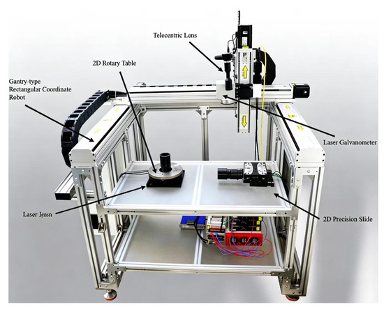
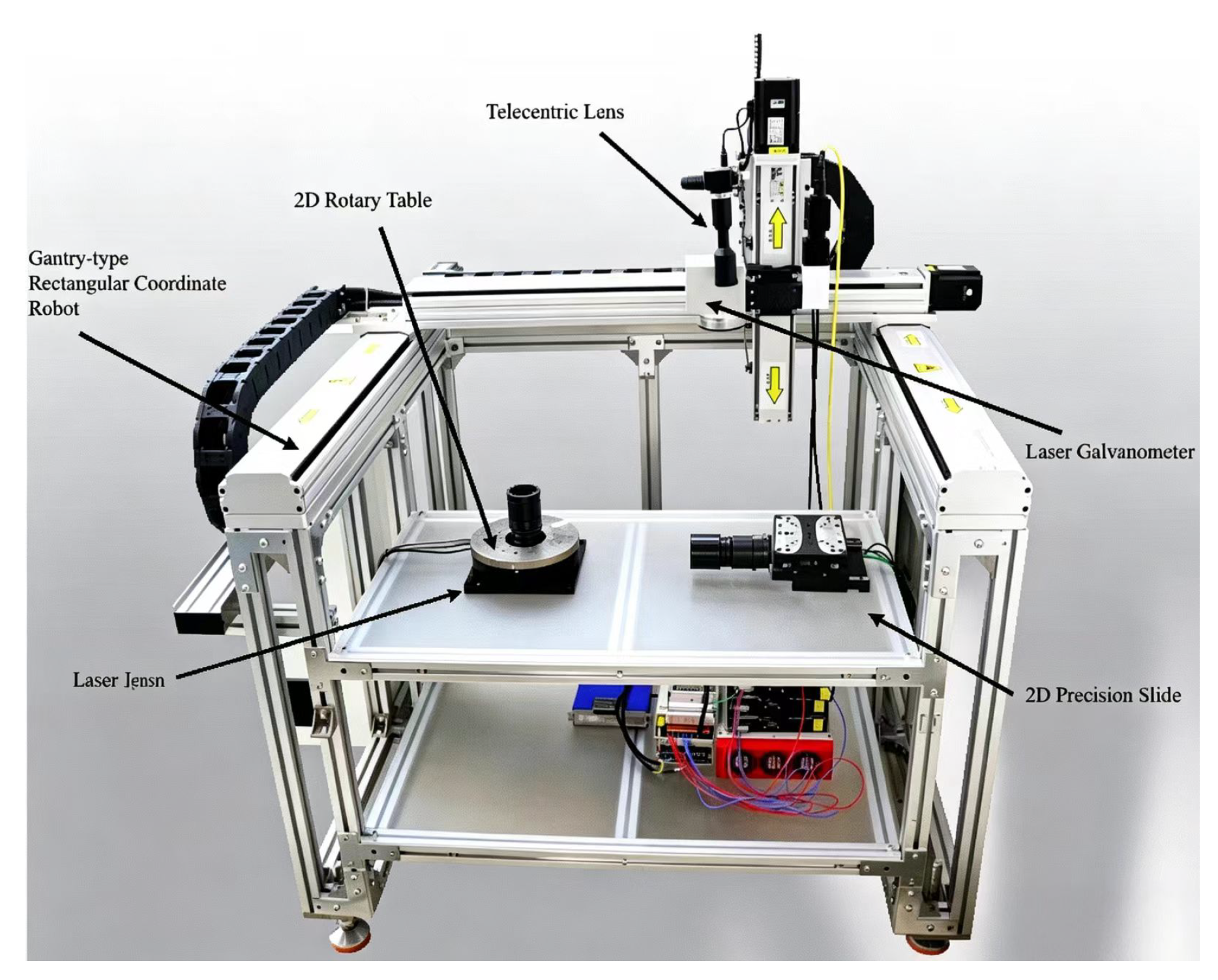
To verify the effectiveness and reliability of the proposed control algorithm, this study takes the precision collaborative machining experimental platform shown in Figure 1 as an experimental object and focuses on the linear interconnection characteristics between the two subsystems of the platform (with coupling order L = 2).

Figure 1. Precision collaborative machining experimental platform.

5.1. Test Platform Specification

The experimental platform system is shown in Figure 1 and consists of five main functional modules. This experiment focuses on the synergistic machining performance of laser galvanometer and the 2D precision slide. Among them, the detector-type vibrating mirror system contains two sets of mirrors in the x-axis and y-axis, and by precisely controlling the rotation angle of the mirrors, the precise positioning of the laser beam can be realized so as to complete the fine laser processing. The 2D precision slide is driven by a direct-drive, iron-core linear motor with a travel of ±30 mm and an external dimension of 125 mm × 125 mm × 60 mm. The platform is designed with crossed roller guideways to provide excellent load carrying capacity and low friction performance.

The laser galvanometer can be described by the following transfer function

$$G_0\left(s\right)={\displaystyle \frac{7.8\times {10}^8}{s^2+6.2\times {10}^{3}s+1.79\times {10}^4}},G_1\left(s\right)={\displaystyle \frac{0.5}{s(0.03s+1){(0.00167s+1)}^{\prime }}}.$$

(61)

The transfer function characterizing the 2D precision slide dynamics is expressed as

$$G_2\left(s\right)={\displaystyle \frac{0.04}{s}},G_3\left(s\right)={\displaystyle \frac{0.05}{s}}.$$

(62)

In Equation (1), the spatial index $i=1,2$ denotes the laser galvanometer and the 2D precision slide, respectively. The state $x_1\left(p\right)$ is the galvanometer angle, $x_2\left(p\right)$ is the slide displacement, $y_1\left(p\right)$ is the laser spot position, and $y_2\left(p\right)$ is the slide position. The coupling signals $v_i\left(p\right),w_i\left(p\right)$ represent the mechanical and optical interactions between the two subsystems and are estimated via Equation (8).

The continuous transfer functions $G_0\left(s\right),G_1\left(s\right),G_2\left(s\right),G_3\left(s\right)$ in Equations (61) and (62) are the dynamic models of the precision machining platform corresponding to the general state-space form in Equation (1). They are converted to discrete-time state-space models via the ZOH method with sampling time $T_s=0.01$ s, and the resulting matrices are used in Equation (1).

Then, through the model reformulation described in Section 2.2, the augmented matrices in Equation (5) are obtained as follows:

$$A_{TT}=\left[\begin{array}{ccc}1.607& 1& 0\\ -0.6086& 0& 0\\ 0& 0& 1\end{array}\right],B_{TU}=\left[\begin{array}{cc}1.239& 0\\ -0.009282& 0\\ 0& 0.0004\end{array}\right],C_T=\left[\begin{array}{ccc}1& 0& 0\\ 0& 0& 1\end{array}\right].$$

$$A_{TS}=\left[\begin{array}{cc}0.05& 0\\ 0& 0\\ 0.03& 0\end{array}\right],A_{ST}=\left[\begin{array}{ccc}0.05& 0& 0.03\\ 0& 0& 0\end{array}\right],A_{SS}=0.$$

The matrices $E_1$, $E_2$, $F_1$, $F_2$ are determined based on the physical characteristics of the precision machining platform. The uncertainty bounds are set based on the identified variations in the system parameters, which reflect typical manufacturing tolerances and environmental variations in the experimental platform. The numerical values used in this paper are

$$E_1=\left[\begin{array}{ccc}1& 0& 0\\ 0& 1& 0\\ 0& 0& 0\end{array}\right],F_1=\left[\begin{array}{ccc}0.0804& 0& 0\\ -0.0304& 0& 0\\ 0& 0& 0\end{array}\right],E_2=\left[\begin{array}{ccc}0.05& 0& 0\end{array}\right],F_2=\left[\begin{array}{cc}0.062& 0\\ -0.0464& 0\\ 0& 0\end{array}\right].$$

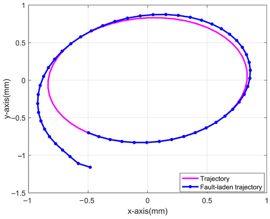
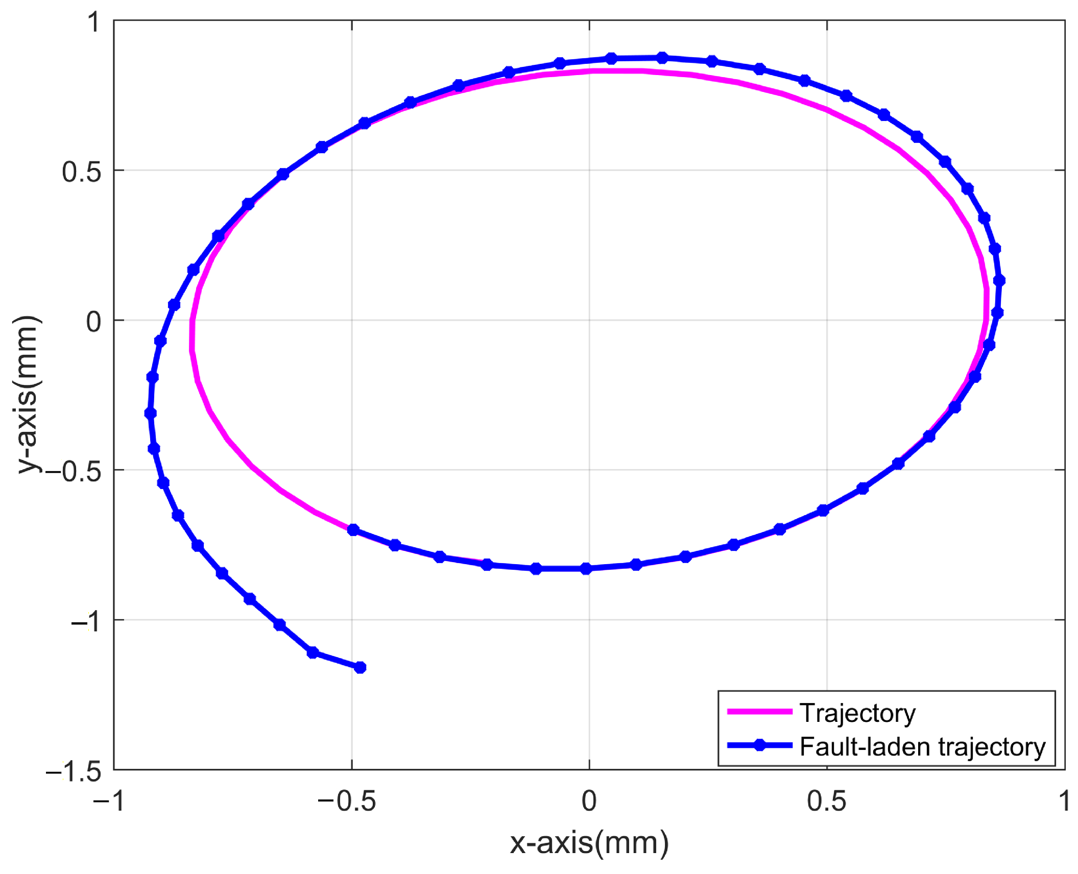
Using $G_0\left(s\right)$ and $G_2\left(s\right)$, the normal trajectory is shown by the pink line in Figure 2; under actuator fault and interference conditions, the trajectory becomes the blue line. The observed deviation and large tracking error indicate that faults and disturbances must be considered in such a complex system.

Figure 2. Normal trajectory and faulty trajectories.

5.2. FTC of Subsystem Laser Galvanometer

The required reference trajectory for the laser galvanometer subsystem is defined as

$$Y_{ref1}=0.5{(sin\left(3p\right)+sin\left(15p\right))}^2.$$

(63)

The actuator faults were emulated through the host computer control system, with the fault parameters configured as follows:

$${\Gamma }_1=0.85+0.15sin\left(2\pi p\right).$$

(64)

The dynamic regulation capability of the controller was evaluated by introducing large-magnitude faults as defined in Equation (64). The fault tolerance performance, ensured through both frequency-domain design and learning gain adaptation, remains effective regardless of the fault amplitude.

The external interference signal is defined as

$$w=1.5sin(2\pi p-0.34\pi ).$$

(65)

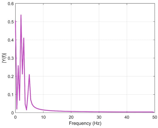
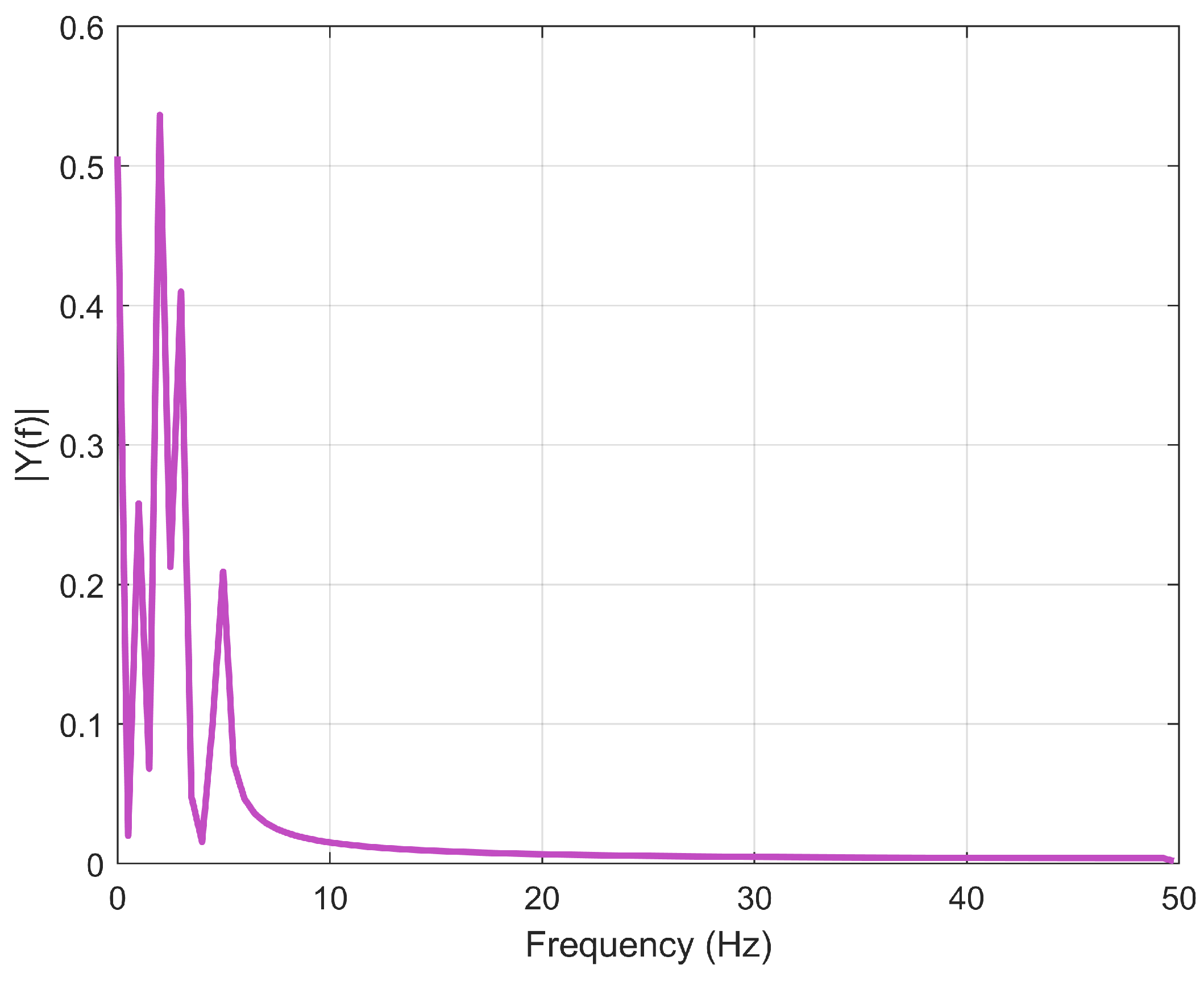
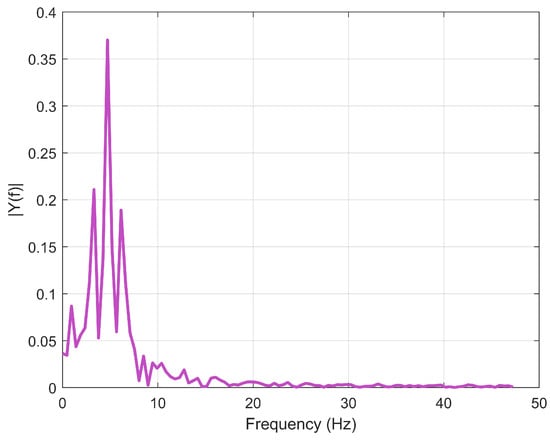
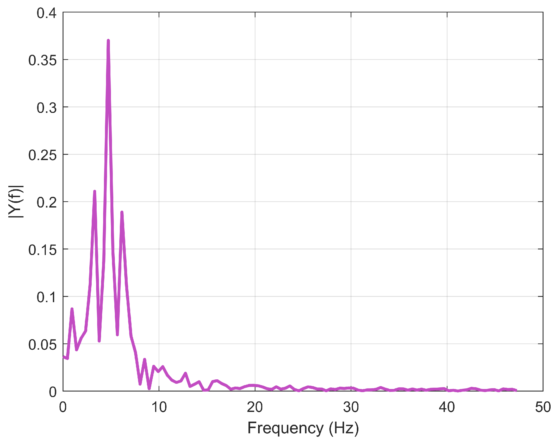
The gain matrices are solved by utilizing the MATLAB toolbox. Through the model reformulation described in Section 2.2, the original space-time description has been converted into a time-iteration model suitable for ILC design. According to the reference trajectory (63) shown in Figure 3, its main frequency motion range is from 0 to 10 $\mathrm{Hz}$, which belongs to low frequency range. Based on Theorem 4, the gain matrix of the finite-frequency-domain FTC is obtained as

$${\mathrm{K}}_{11}=[-1.3735-0.8083],{\mathrm{K}}_{21}=0.3256,{\mathrm{K}}_{31}=0.0248.$$

Figure 3. Subsystem laser galvanometer expects a spectrum of output trajectories.

To improve the assessment of fault estimation validity and accuracy at each iteration, this paper introduces the Root Mean Square (RMS) error as a measure of fault estimation error. The RMS metric serves as a comprehensive fault estimation evaluation tool that quantifies error amplitudes while identifying large-deviation risks and maintaining direct correlation with signal energy. These combined characteristics not only satisfy stringent engineering precision requirements but also establish rigorous quantitative criteria to guide iterative optimization processes in control systems. It is defined as follows:

$$RMS=\sqrt{{\displaystyle \frac{1}{T}}{\displaystyle \sum _{p=1}^T}{e^2}_l\left(p\right)}.$$

(66)

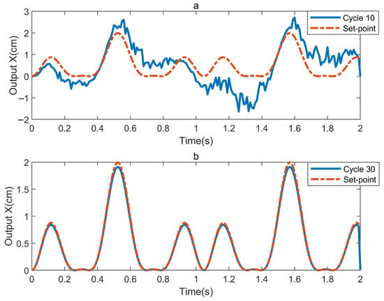
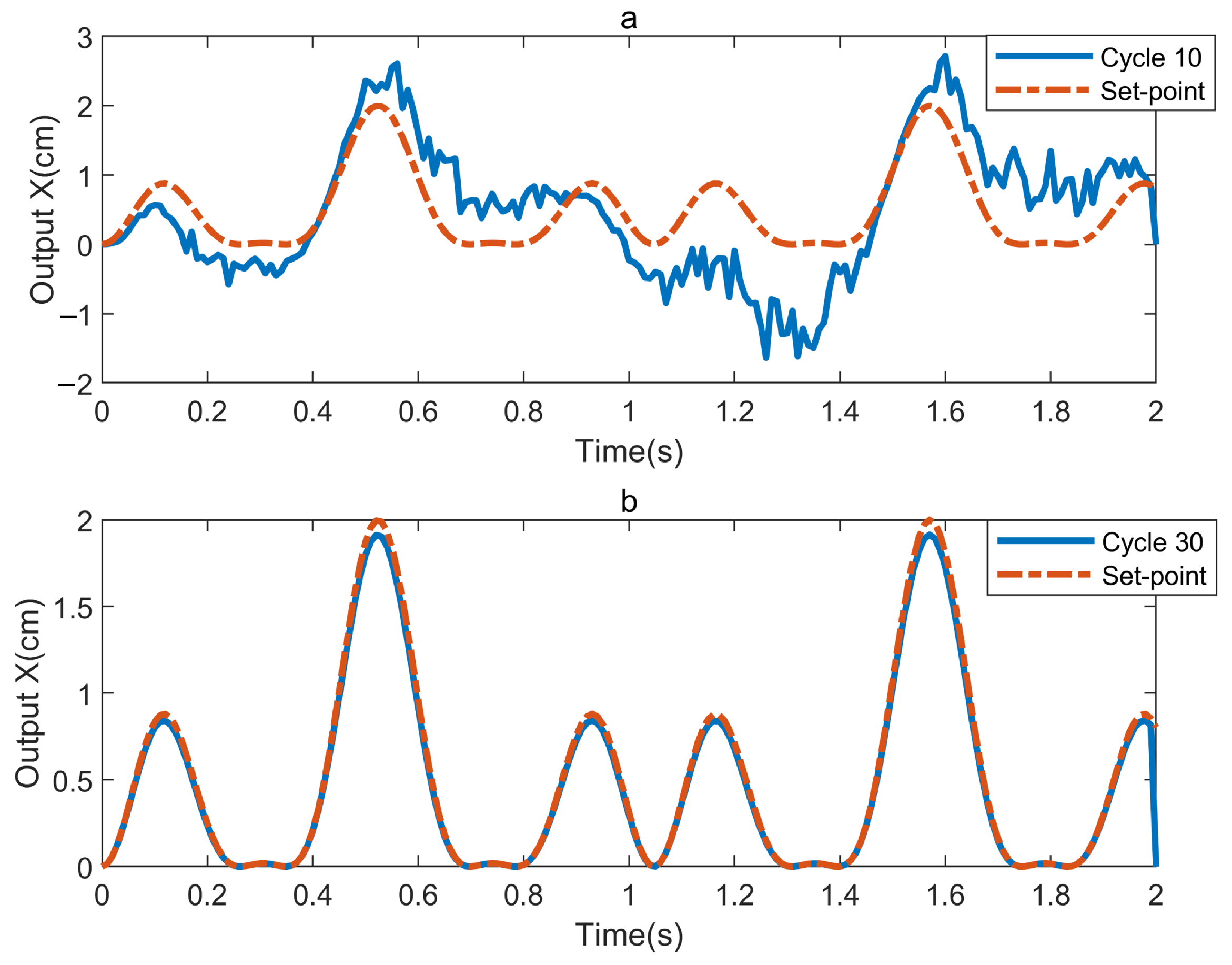
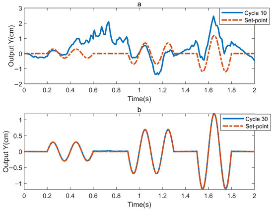
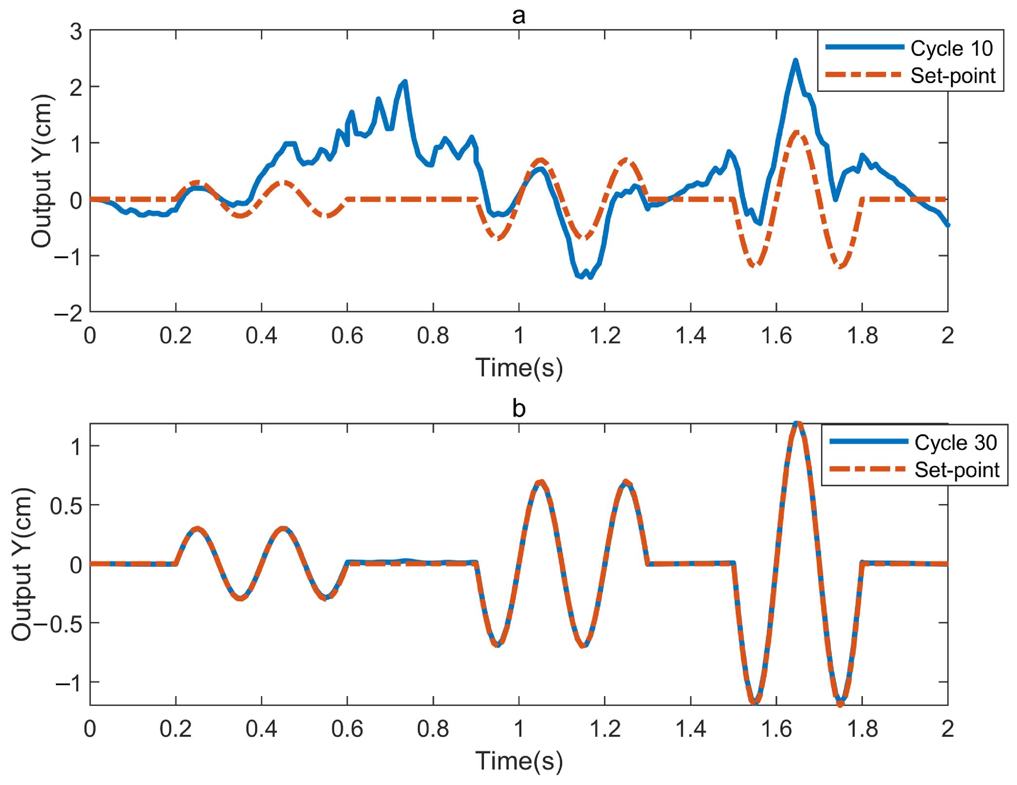
Figure 4 presents the output trajectories of the subsystem in different iterations in the absence of fault signaling (Equation (64)), considering only external disturbances (Equation (65)). The results demonstrate that the proposed algorithm achieves precise trajectory tracking by the 30th iteration, exhibiting satisfactory tracking performance.

Figure 4. Experimental results for $Y_{ref1}$. (a) represents the 10th trial; (b) represents the 30th trial.

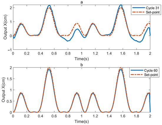
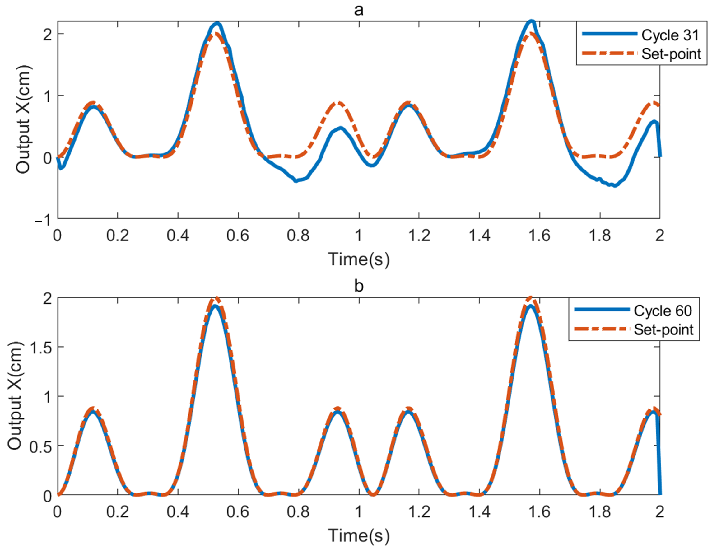
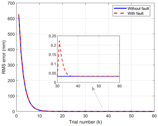
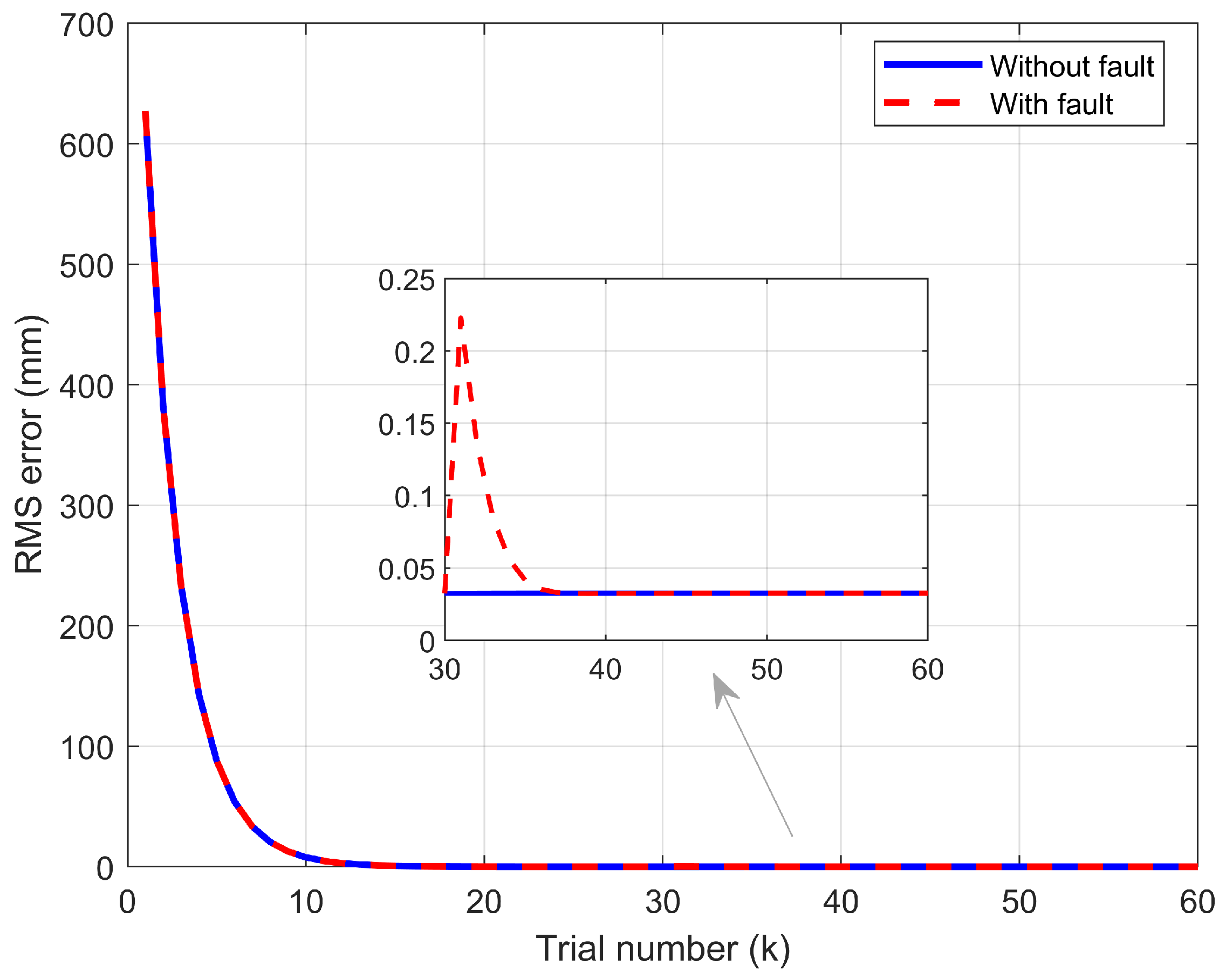
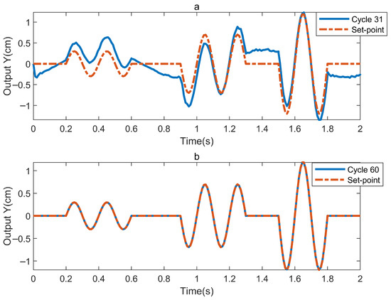
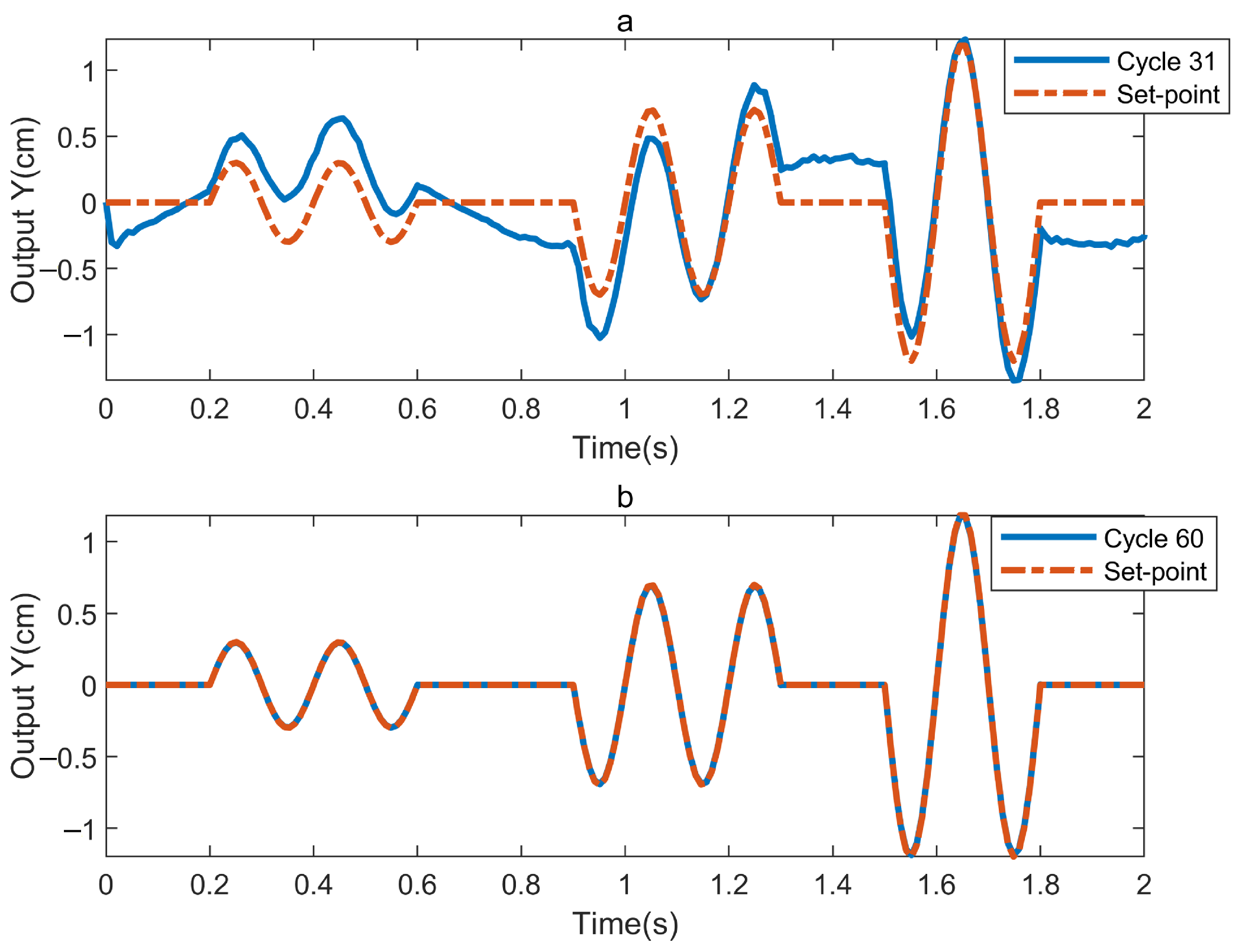
Figure 5 illustrates that when the actuator of the subsystem suddenly fails at the 31st iteration with the fault parameter Equation (64), the output trajectory of the subsystem then transforms from the stable convergence state in Figure 4b and Figure 5a. Due to the fault, the tracking accuracy decreases significantly. The tracking error increases after 1.8 s due to the activation of the time-varying actuator fault defined in Equation (64) at the 31st iteration. However, with the increase in k, the tracking performance of the subsystem gradually recovers, and eventually it can accurately track the desired trajectory, as shown in Figure 5b. This indicates that the control algorithm has good fault tolerance. Figure 6 presents the evolution of output displacement as a function of the trial number under both fault-free and faulty conditions. It can be observed that, in the absence of actuator faults, the output displacement converges to zero within 30 iterations. When a fault is introduced, the output temporarily deviates but subsequently recovers and converges to zero within 60 iterations, demonstrating the effectiveness of the proposed fault-tolerant control scheme.

Figure 5. Experimental results for $Y_{ref1}$. (a) represents the 31st trial; (b) represents the 60th trial.

Figure 6. Error convergence comparison.

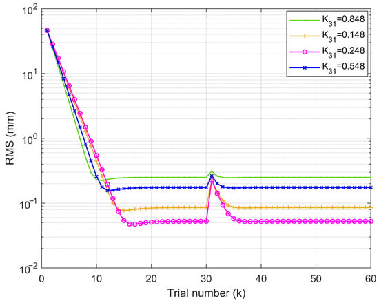
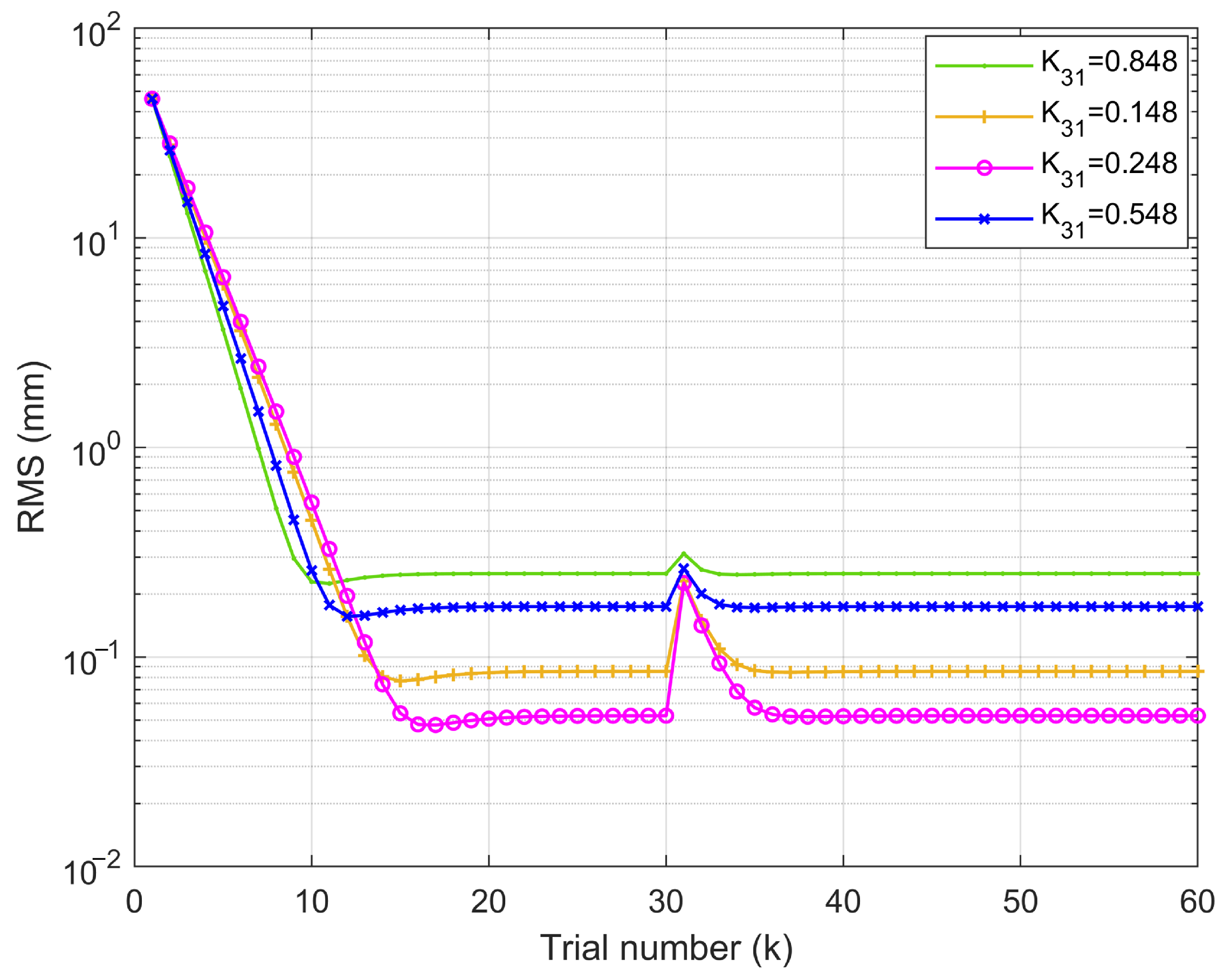
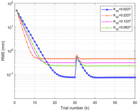
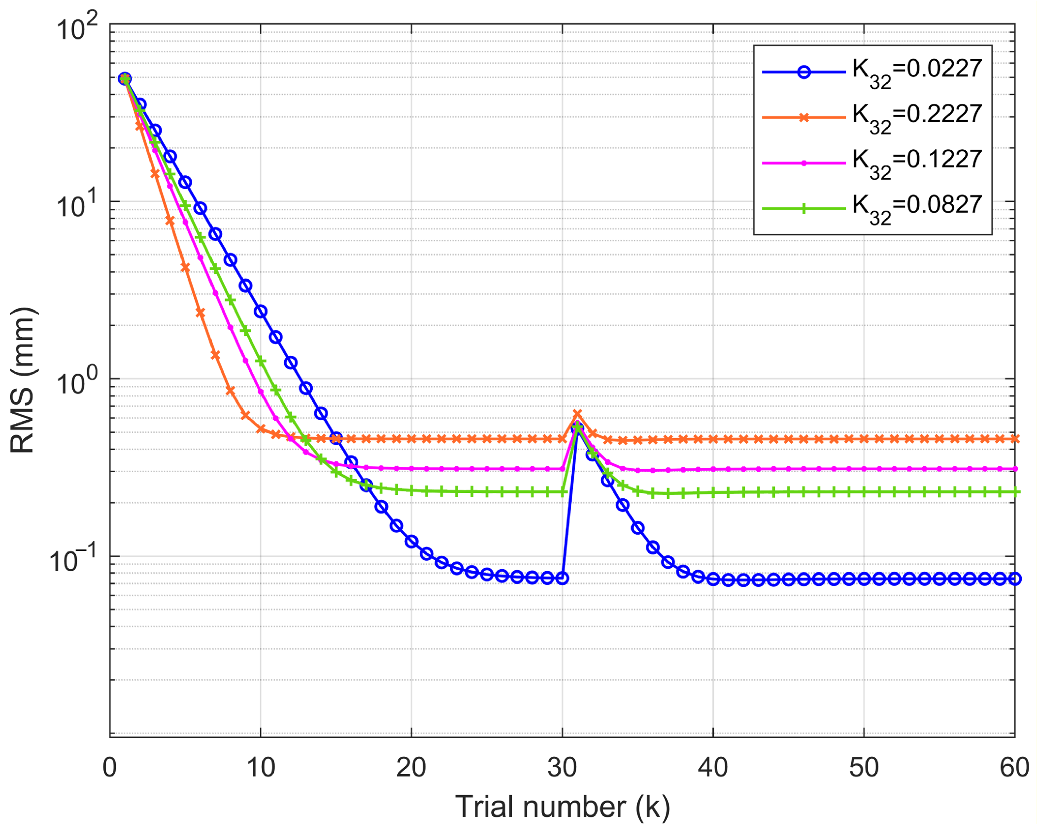
Figure 7 illustrates the error effect of the subsystem under actuator failure conditions. The curves clearly demonstrate that the designed fault-tolerant technique is able to repair faults accurately and efficiently as they change, with the best convergence at $K_{31}=0.248$.

Figure 7. Different convergence errors from different FTC parameters $K_{31}$.

5.3. FTC of Subsystem 2D Precision Slide

To fully verify the validity of fault-tolerance performance, the required reference trajectory of the subsystem 2D precision slide is defined as a segmented function, $p\in \left[0,2\right]$

$$y_{ref2}=\left\{\begin{array}{cc}sin\left(10\pi p\right)& 0.2\le p<0.6,\\ 2sin\left(10\pi p\right)& 0.9\le p<1.3,\\ 3sin\left(10\pi p\right)& 1.5\le p<1.8,\\ 0& others.\end{array}\right.$$

(67)

The actuator failure factor is set to

$${\Gamma }_2=0.75+0.15sin\left(0.02\pi p\right).$$

(68)

The noise interference signal is reinitialized to

$$w=1.5sin(2\pi p-0.34\pi ).$$

(69)

Similarly, the gain matrix of the FTC is obtained as

$${\mathrm{K}}_{12}=[-1.6282-0.8017],{\mathrm{K}}_{22}=0.3033,{\mathrm{K}}_{32}=0.0227.$$

Figure 8 illustrates the spectrogram of the desired trajectory of the subsystem, while its trajectory in the time domain range is shown as the red line in Figure 9. Figure 9 depicts the tracking curves when the system is disturbed only by noise interference (69) and not by fault signals (68), showing the output trajectories at the 10th and 30th iterations, respectively, from which the convergence trend of the output trajectories can be observed. Figure 10, on the other hand, reflects the sudden failure of the actuator of the subsystem at the 31st iteration with the fault parameter (68). As a result of this fault, the tracking accuracy of the subsystem decreases significantly (Figure 10a). However, the subsystem is eventually able to track the desired trajectory accurately, as shown in Figure 10b.

Figure 8. Subsystem 2D precision slide expects a spectrum of output trajectories.

Figure 9. Experimental results for $Y_{ref2}$. (a) represents the 10th trial; (b) represents the 30th trial.

Figure 10. Experimental results for $Y_{ref2}$. (a) represents the 31st trial; (b) represents the 60th trial.

Figure 11 clearly demonstrates the gradual convergence of the proposed method as the number of iterations increases, indicating that the FTC is effective. Specifically, when $K_{32}=0.0227$, the system achieves highest convergence accuracy through iterations, exhibiting optimal convergence performance. In contrast, when $K_{32}=0.2227$, the convergence accuracy shows significant degradation. These experimental results validate that $K_{32}=0.0227$, as theoretically derived in this work, represents the optimal parameter selection.

Figure 11. Different convergence errors from different FTC parameters $K_{32}$.

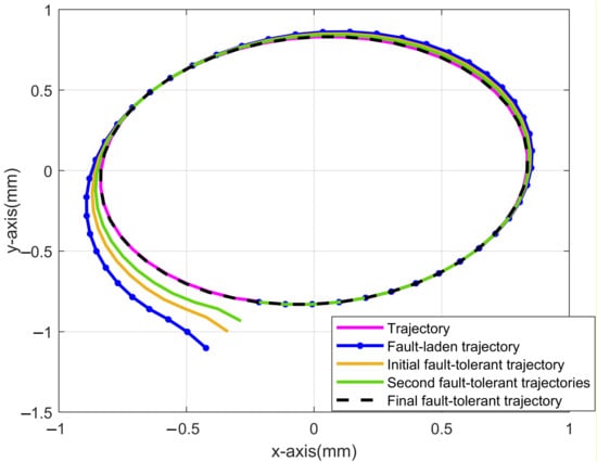
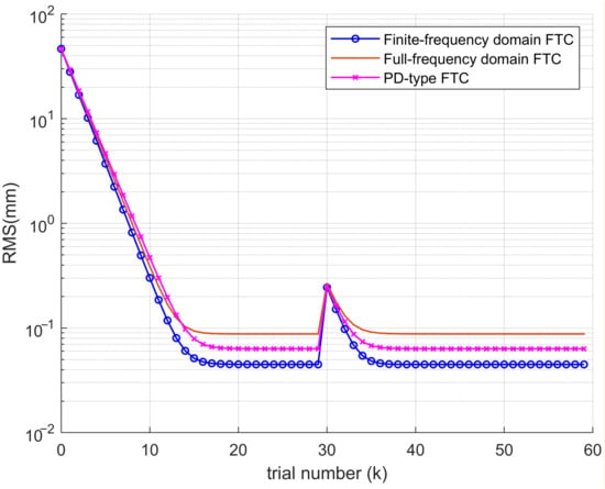
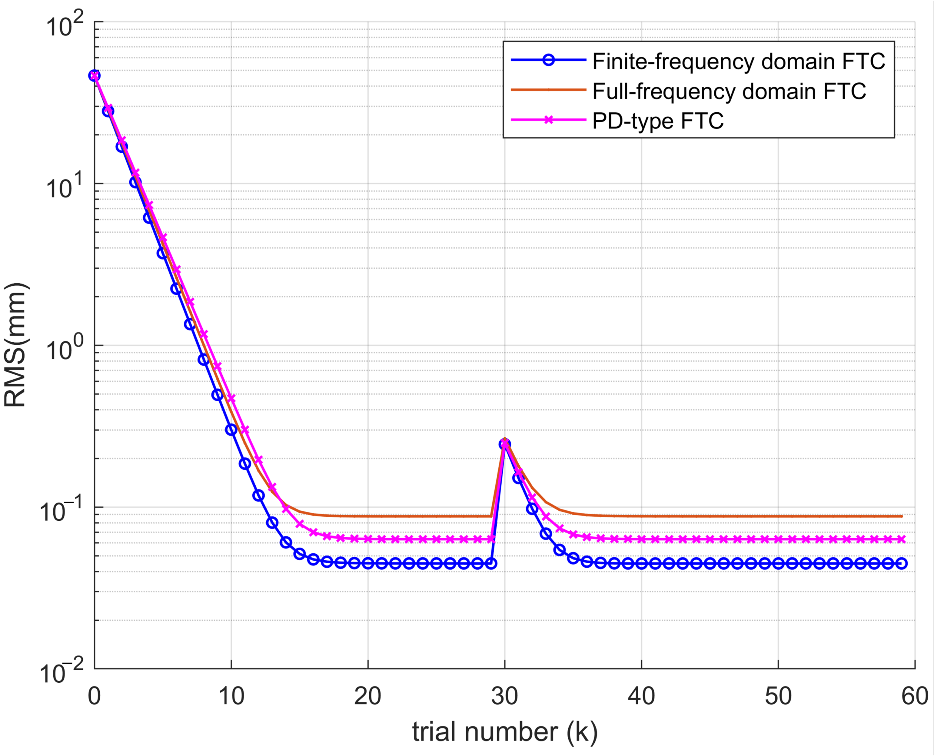
Figure 12 demonstrates that, when two interconnected subsystems are in motion (black line), the subsystem FTC can restore the system to the correct trajectory despite actuator failures and external disturbances. Figure 13 presents the tracking error performance curves for three FTC methods: PD-type ILC (pure time-domain baseline), full-frequency FTC-ILC (stability constraints across all frequencies), and the proposed finite-frequency FTC-ILC. Although all three methods achieve error convergence, the ILC method operating in the finite-frequency-domain yields faster tracking error convergence and more accurate system output tracking. These results confirm the feasibility and effectiveness of the proposed finite-frequency-domain FTC design.

Figure 12. Interconnected system outputs showing normal traces, fault traces, and fault-tolerant adjustment traces.

Figure 13. Frequency domain and finite-frequency-domain fault tolerance comparison test.

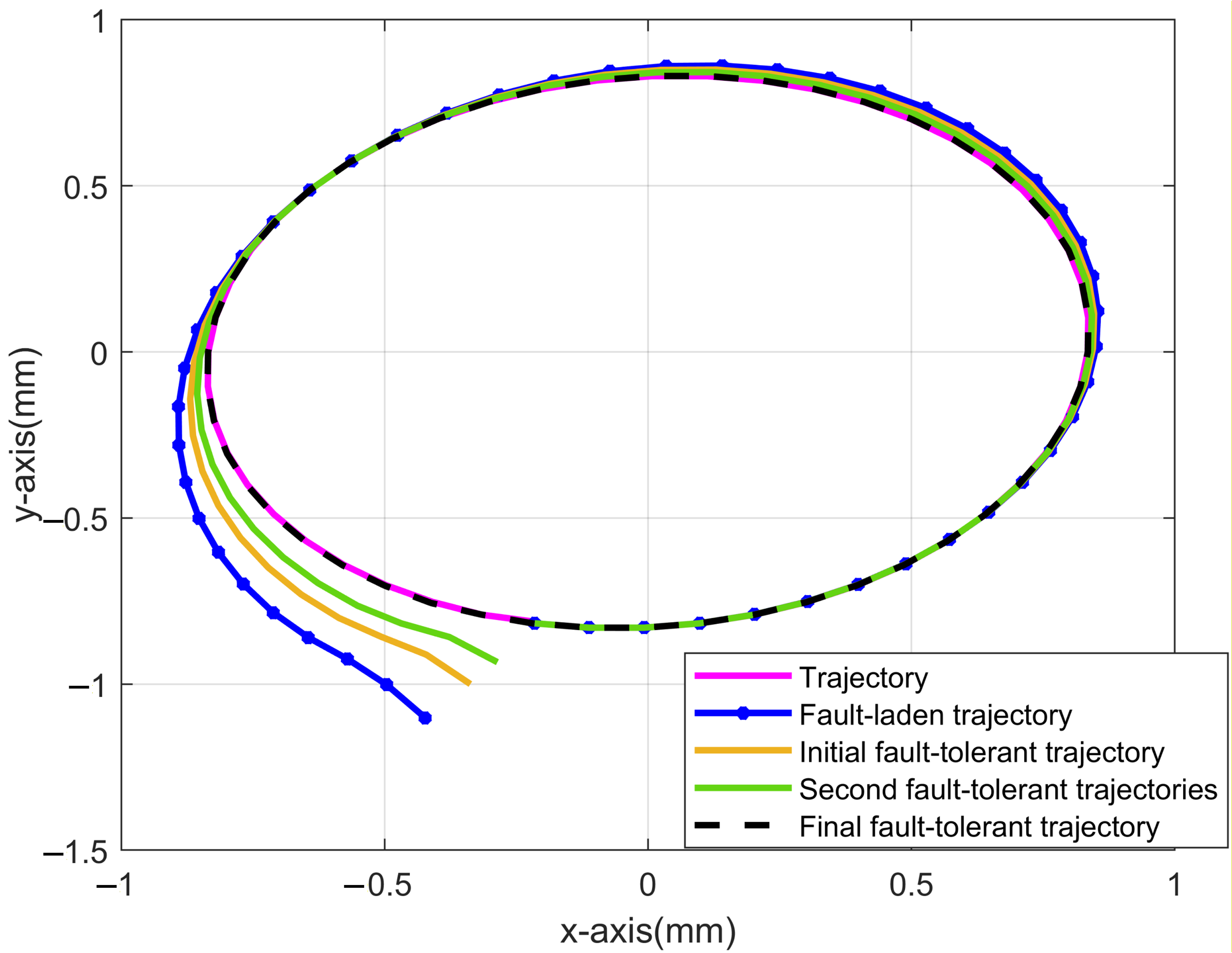
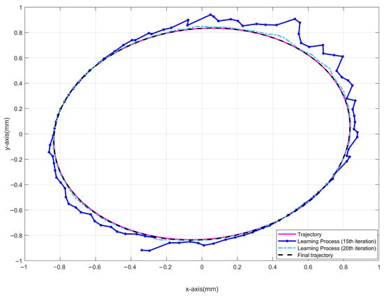
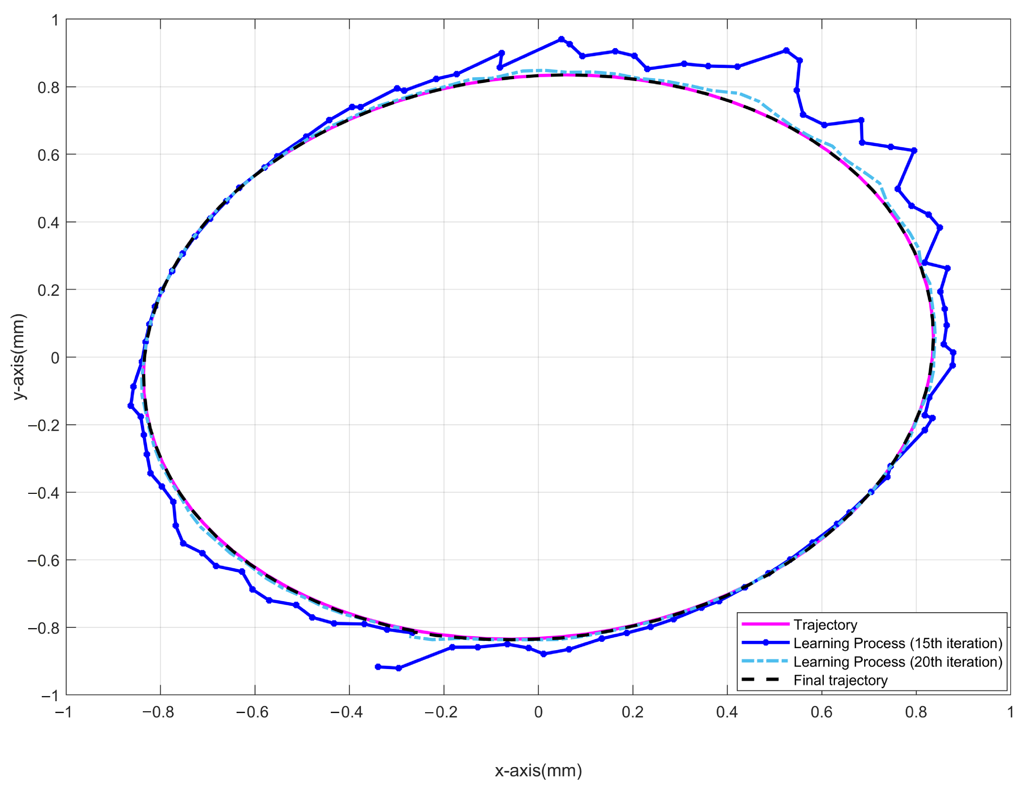
Figure 14 presents the dynamic response characteristics of the system under non-repetitive disturbance conditions. The trajectory at the 15th iteration exhibits significant oscillations and steady-state deviation, indicating the initial learning phase. The trajectory at the 20th iteration demonstrates markedly improved convergence with substantially reduced tracking errors. The final trajectory forms an ideal closed loop, thereby validating the effectiveness of the proposed methodology.

Figure 14. System non-repetitive disturbance test.

6. Conclusions and Future Work

This paper investigated actuator faults and external disturbances in spatially interconnected discrete systems. By eliminating the interconnection variables from a two-dimensional state-space model, a one-dimensional equivalent model was derived. Using repetitive process theory, an ILC algorithm was designed to transform the controlled system into a repetitive process model. Combined with the generalized KYP lemma, stability conditions for different frequency ranges were established, along with sufficient conditions for asymptotic convergence of the tracking error. The proposed fault-tolerant algorithm was validated experimentally on a precision collaborative machining platform.

The current experimental validation is limited to two-dimensional spatially interconnected systems. Future work will focus on extending the approach to higher-dimensional systems, integrating adaptive control techniques for dynamic environments and investigating robust ILC methods for spatially interconnected systems subject to non-repetitive perturbations and uncertainties on physical platforms. This paper adopts the standard ILC assumption that the initial state is reset at the beginning of each iteration. Issues such as significant initial state mismatches and adaptive gain tuning are not fully addressed here. Future research will focus on extending the proposed method to handle non-repetitive initial conditions and developing adaptive mechanisms for gain tuning, as well as further validating robust ILC methods on physical systems.

References

- Huang, S.; Zeng, Z.; Ota, K.; Dong, M.; Wang, T.; Xiong, N.N. An intelligent collaboration trust interconnections system for mobile information control in ubiquitous 5G networks. IEEE Trans. Netw. Sci. Eng. 2020, 8, 347–365. [Google Scholar] [CrossRef] [Scilit]
- An, L.; Yang, G.H. Decentralized adaptive fuzzy secure control for nonlinear uncertain interconnected systems against intermittent DoS attacks. IEEE Trans. Cybern. 2018, 49, 827–838. [Google Scholar] [CrossRef] [Scilit]
- Leitão, D.; Cunha, R.; Lemos, J.M. Adaptive control of quadrotors in uncertain environments. Eng 2024, 5, 544–561. [Google Scholar] [CrossRef] [Scilit]
- Xu, S.; Wang, L.; Dai, H.; Wang, H.; Chen, H.; Chai, Y.; Zheng, W.X. A segmented iterative learning scheme-based distributed fault estimation for switched interconnected nonlinear systems. IEEE Trans. Neural Netw. Learn. Syst. 2024, 36, 6612–6626. [Google Scholar] [CrossRef] [Scilit]
- Liang, J.; Wu, J.; Wang, Y.; Zhong, Z.; Bai, X. Sensorless Control for a Permanent Magnet Synchronous Motor Based on a Sliding Mode Observer. Eng 2024, 5, 1737–1751. [Google Scholar] [CrossRef] [Scilit]
- Polyak, B.T.; Khlebnikov, M.V.; Shcherbakov, P.S. Linear matrix inequalities in control systems with uncertainty. Autom. Remote Control 2021, 82, 1–40. [Google Scholar] [CrossRef] [Scilit]
- Chibani, A.; Chadli, M.; Shi, P.; Braiek, N.B. Fuzzy fault detection filter design for T–S fuzzy systems in the finite-frequency domain. IEEE Trans. Fuzzy Syst. 2016, 25, 1051–1061. [Google Scholar] [CrossRef] [Scilit]
- Chi, R.; Zhang, H.; Huang, B.; Hou, Z. Quantitative data-driven adaptive iterative learning control: From trajectory tracking to point-to-point tracking. IEEE Trans. Cybern. 2020, 52, 4859–4873. [Google Scholar] [CrossRef] [Scilit]
- Spiegel, I.A.; Strijbosch, N.; de Rozario, R.; Oomen, T.; Barton, K. Stable inversion of piecewise affine systems with application to feedforward and iterative learning control. IEEE Trans. Autom. Control 2024, 69, 6836–6851. [Google Scholar] [CrossRef] [Scilit]
- Chen, Y.; Chu, B.; Freeman, C.T. Iterative learning control for path-following tasks with performance optimization. IEEE Trans. Control Syst. Technol. 2021, 30, 234–246. [Google Scholar] [CrossRef] [Scilit]
- Angelini, G.; Corsini, A.; Delibra, G.; Tieghi, L. Exploration of axial fan design space with data-driven approach. Int. J. Turbomach. Propuls. Power 2019, 4, 11. [Google Scholar] [CrossRef] [Scilit]
- Sammons, P.M.; Hoelzle, D.; Barton, K. Time-scale transformed iterative learning control for a class of nonlinear systems with uncertain trial duration. IEEE Trans. Control Syst. Technol. 2019, 28, 1972–1979. [Google Scholar] [CrossRef] [Scilit]
- Sun, Y.; Tao, H.; Stojanovic, V. Autoregressive data generation method based on wavelet packet transform and cascaded stochastic quantization for bearing fault diagnosis under unbalanced samples. Eng. Appl. Artif. Intell. 2024, 138, 109402. [Google Scholar] [CrossRef] [Scilit]
- Lai, J.; Weng, D.; Xian, F.; Xie, Y.; Chen, Y.; Zhou, Q.; Yuan, C. A Hybrid Optimization Model for Transformer Fault Diagnosis Based on Gas Classification. Digital 2026, 6, 24. [Google Scholar] [CrossRef] [Scilit]
- Tao, H.; Paszke, W.; Rogers, E.; Yang, H.; Gałkowski, K. Iterative learning fault-tolerant control for differential time-delay batch processes in finite frequency domains. J. Process Control 2017, 56, 112–128. [Google Scholar] [CrossRef] [Scilit]
- Watson, J.D.; Lestas, I. Control of interlinking converters in hybrid AC/DC grids: Network stability and scalability. IEEE Trans. Power Syst. 2020, 36, 769–780. [Google Scholar] [CrossRef] [Scilit]
- Chen, Y.; Chu, B.; Freeman, C.T. A coordinate descent approach to optimal tracking time allocation in point-to-point ILC. Mechatronics 2019, 59, 25–34. [Google Scholar] [CrossRef] [Scilit]
- Zhang, K.; Jiang, B.; Chen, M.; Yan, X.G. Distributed fault estimation and fault-tolerant control of interconnected systems. IEEE Trans. Cybern. 2019, 51, 1230–1240. [Google Scholar] [CrossRef] [Scilit]
- Liang, D.; He, Z.; Ding, S.; Yang, Y. Distributed fault estimation and fault-tolerant control of interconnected systems with plug-and-play features. IEEE Trans. Circuits Syst. I Regul. Pap. 2023, 71, 431–442. [Google Scholar] [CrossRef] [Scilit]
- Song, X.; Man, J.; Ahn, C.K. Joint state and fault estimation for networked interconnected PDE systems with semi-Markov fault coefficient via conjunct measurement. IEEE Trans. Circuits Syst. I Regul. Pap. 2021, 68, 3869–3880. [Google Scholar] [CrossRef] [Scilit]
- Chen, L.; Zhao, Y.; Fu, S.; Liu, M.; Qiu, J. Fault estimation observer design for descriptor switched systems with actuator and sensor failures. IEEE Trans. Circuits Syst. I Regul. Pap. 2018, 66, 810–819. [Google Scholar] [CrossRef] [Scilit]
- Garbouj, Y.; Dinh, T.N.; Raissi, T.; Zouari, T.; Ksouri, M. Optimal interval observer for switched Takagi–Sugeno systems: An application to interval fault estimation. IEEE Trans. Fuzzy Syst. 2020, 29, 2296–2309. [Google Scholar] [CrossRef] [Scilit]
- Sun, S.; Zhang, H.; Zhang, J.; Zhang, K. Fault estimation and tolerant control for discrete-time multiple delayed fuzzy stochastic systems with intermittent sensor and actuator faults. IEEE Trans. Cybern. 2020, 51, 6213–6225. [Google Scholar] [CrossRef] [Scilit]
- Amin, A.A.; Irfan, M.; Waseem, S.; Mubarak, A.; Alwadie, H.; Al Dawsari, S. Application of advanced fault-tolerant control techniques in the design of modern electric vehicles for increased reliability: A review. Automatika 2026, 67, 237–265. [Google Scholar] [CrossRef] [Scilit]
- Radhika, T.; Chandrasekar, A.; Lee, Y.C.; Subhashri, A.; Shamrooz, M.A.; Chang, W.J. Fault–Tolerant State Estimation Synthesis For Competitive Neural Networks Subject to Deception Attacks Using Probabilistic Time Varying Delay. J. Frankl. Inst. 2026, 363, 108679. [Google Scholar] [CrossRef] [Scilit]
- Gong, J.; Ma, Y.; Jiang, B.; Zhang, Y.; Guo, L. An adaptive fault-tolerant control scheme for heterogeneous multiagent systems. IEEE Trans. Syst. Man. Cybern. Syst. 2024, 55, 1264–1276. [Google Scholar] [CrossRef] [Scilit]
- Zhang, J.; Ma, L.; Zhao, J.; Zhu, Y. Fault detection and fault-tolerant control for discrete-time multiagent systems with sensor faults: A data-driven method. IEEE Sens. J. 2024, 24, 22601–22609. [Google Scholar] [CrossRef] [Scilit]
- de Rozario, R.; Oomen, T. Frequency response function-based learning control: Analysis and design for finite-time convergence. IEEE Trans. Autom. Control 2022, 68, 1807–1814. [Google Scholar] [CrossRef] [Scilit]
- Ge, Y.; Sheng, Z.; Fang, Y.; Zhang, L. An AFD-based ILC dynamics adaptive matching method in frequency domain for distributed consensus control of unknown multiagent systems. IEEE Trans. Circuits Syst. I Regul. Pap. 2022, 69, 3366–3378. [Google Scholar] [CrossRef] [Scilit]
- Boeren, F.; Bareja, A.; Kok, T.; Oomen, T. Frequency-domain ILC approach for repeating and varying tasks: With application to semiconductor bonding equipment. IEEE/ASME Trans. Mechatron. 2016, 21, 2716–2727. [Google Scholar] [CrossRef] [Scilit]
- Morales, A.; Agili, S.S.; Meklachi, T. S-parameter sampling in the frequency domain and its time-domain response. IEEE Trans. Instrum. Meas. 2020, 70, 6501113. [Google Scholar] [CrossRef] [Scilit]
- Rodríguez-Fernández, J.; González-Prelcic, N.; Venugopal, K.; Heath, R.W. Frequency-domain compressive channel estimation for frequency-selective hybrid millimeter wave MIMO systems. IEEE Trans. Wirel. Commun. 2018, 17, 2946–2960. [Google Scholar] [CrossRef] [Scilit]
- Chen, H.; Xu, R.; Tang, Y.; Long, X. Fault-tolerant iterative learning control for batch processes with time-varying state delays and uncertainties. Int. J. Syst. Sci. 2023, 54, 2423–2441. [Google Scholar] [CrossRef] [Scilit]
- Aarnoudse, L.; Oomen, T. Model-free learning for massive MIMO systems: Stochastic approximation adjoint iterative learning control. IEEE Control Syst. Lett. 2020, 5, 1946–1951. [Google Scholar] [CrossRef] [Scilit]
- Chen, Y.; Freeman, C.T. Iterative learning control for piecewise arc path tracking with validation on a gantry robot manufacturing platform. ISA Trans. 2023, 139, 650–659. [Google Scholar] [CrossRef] [Scilit]
- Wang, L.; Huangfu, Z.; Li, R.; Wen, X.; Sun, Y.; Chen, Y. Iterative learning control with parameter estimation for non-repetitive time-varying systems. J. Frankl. Inst. 2024, 361, 1455–1466. [Google Scholar] [CrossRef] [Scilit]
- Jonnalagadda, V.K.; Elumalai, V.K. Hardware-in-the-loop testing of current cycle feedback ILC for stabilisation and tracking control of under-actuated visual servo system. Int. J. Syst. Sci. 2021, 52, 1042–1060. [Google Scholar] [CrossRef] [Scilit]
- Chen, Y.; Chu, B.; Freeman, C.T. Iterative learning control for robotic path following with trial-varying motion profiles. IEEE/ASME Trans. Mechatron. 2022, 27, 4697–4706. [Google Scholar] [CrossRef] [Scilit]
- Zhao, Z.; Wang, J.; Tao, Q.; Li, A.; Chen, Y. An unknown wafer surface defect detection approach based on incremental learning for reliability analysis. Reliab. Eng. Syst. Saf. 2024, 244, 109966. [Google Scholar] [CrossRef] [Scilit]
- Deutschmann-Olek, A.; Stadler, G.; Kugi, A. Stochastic iterative learning control for lumped-and distributed-parameter systems: A wiener-filtering approach. IEEE Trans. Autom. Control 2020, 66, 3856–3862. [Google Scholar] [CrossRef] [Scilit]
- Zhou, L.; Tao, H.; Yang, H. Iterative learning control for spatially interconnected systems based on output information. Inf. Control 2020, 49, 274–280. [Google Scholar]
- Tao, H.; Li, X.; Paszke, W.; Stojanovic, V.; Yang, H. Robust PD-type iterative learning control for discrete systems with multiple time-delays subjected to polytopic uncertainty and restricted frequency-domain. Multidimens. Syst. Signal Process. 2021, 32, 671–692. [Google Scholar] [CrossRef] [Scilit]
- Tao, H.; Wei, Q.; Paszke, W.; Zhou, L.; Yang, H. Robust iterative learning control in finite frequency ranges for differential spatially interconnected systems. Circuits Syst. Signal Process. 2020, 39, 5104–5126. [Google Scholar] [CrossRef] [Scilit]
- Tao, H.; Zhou, L.; Hao, S.; Paszke, W.; Yang, H. Output feedback based PD-type robust iterative learning control for uncertain spatially interconnected systems. Int. J. Robust Nonlinear Control 2021, 31, 5962–5983. [Google Scholar] [CrossRef] [Scilit]
- Paszke, W.; Rogers, E.; Gałkowski, K. Experimentally verified generalized KYP lemma based iterative learning control design. Control Eng. Pract. 2016, 53, 57–67. [Google Scholar] [CrossRef] [Scilit]
Disclaimer/Publisher’s Note: The statements, opinions and data contained in all publications are solely those of the individual author(s) and contributor(s) and not of MDPI and/or the editor(s). MDPI and/or the editor(s) disclaim responsibility for any injury to people or property resulting from any ideas, methods, instructions or products referred to in the content. |
© 2026 by the authors. Licensee MDPI, Basel, Switzerland. This article is an open access article distributed under the terms and conditions of the Creative Commons Attribution (CC BY) license.