


Abstract
This study investigates the rotational dynamics of a symmetric rigid body (RB) about a fixed point under the combined effects of a Newtonian force field (NFF), an electromagnetic field (EF), and external torques. A large parameter (LP) approach, together with the averaging method (AM), is used to simplify the nonlinear equations of motion (EOMs). Both analytical and numerical solutions are applied to examine the system behavior under different conditions. The results indicate stable motion within certain parameter ranges, where angular velocity components show either exponential decay or periodic behavior depending on the applied torques. These findings are useful for practical applications, particularly in spacecraft attitude control and other engineering systems involving rotating bodies.
1. Introduction
The rotation of a rigid body (RB) around a fixed point within a uniform or a Newtonian force field (NFF) is a key challenge in classical theoretical mechanics. This analysis requires advanced mathematical techniques, as the motion is dictated by six nonlinear differential equations (DEs) accompanied by three first integrals Amer et al. and Leimanis [1,2,3]. Solutions to these equations exist only in a limited number of special cases [4], characterized by the discovery of a critical fourth integral. These scenarios require certain conditions on the center of mass position and the main moments of inertia to be satisfied. To obtain this integral, several integrable scenarios have been proposed Yehia et al. and Elmandouh [5,6,7,8]. Six cases of integrable RB motion have been found in [5], occurring when a body is subject to a symmetric mix of potential and gyroscopic forces and begins with specific initial conditions. The author also examined generalizations of the Lagrange and Kovalevskaya cases, as well as the complete symmetry one. In [6], a rotational transformation with an angular velocity that varies with position was used to investigate the generalization of the six integrable cases identified earlier. In [7], two new criteria were introduced to identify suitable integrable cases of an RB motion analogous to the Kovalevskaya top. In [8], a novel class of two-dimensional integrable systems characterized by twenty arbitrary parameters was investigated.
Over the past few decades, perturbation methods [9] have attracted significant attention from researchers and can be employed to address the challenges of solving nonlinear ordinary differential equations (DEs), including the approach of small parameter (ASP), the method of Krylov–Bogoliubov–Mitropolski, and the averaging method (AM). In studies [10,11], the approach of small parameter (ASP) was successfully applied to obtain the approximate solutions (ASs) for the rapid spinning motion of an RB under two scenarios: a uniform gravitational field [10] and an NFF [11]. Meanwhile, the solutions obtained in these works contain singularities, which are thoroughly examined in [12,13,14], where the focus shifts to the impact of the gyrostatic moment (GM) on the body, independent of whether it is under a gravitational or Newtonian field. In [15], the ASP was further applied to study the approximate behavior of three-dimensional rotatory motion of an RB exposed to an NFF, a magnetic field, and the GM, with detailed derivations of Euler’s angles. This methodology was adopted in [16] to investigate the body’s motion as it is extended to take magnetization by rotation (Barnett–London effect) into account.
The AM has also been frequently adopted to derive ASs for symmetric bodies rotating about a fixed point within a uniform field [17,18], under the effect of an NFF [19,20], as well as under the action of the GM [21,22], and in the presence of an EF [23]. Specifically, in [21], the study involved a case where the body’s inertia ellipsoid was nearly identical to its rotational ellipsoid, with both uniform and EFs acting on it. The Euler angles in this context were represented as functions of a small parameter and illustrated graphically. Similarly, Panayotounakos and Rizou [22] reduced the ME to a pair of second-order nonlinear DEs that were numerically solved. Likewise, Buck and Hayt [23] derived and numerically solved the averaged ME for an RB analogous to Lagrange’s gyroscope, focusing on certain initial values for the nutation angle and assuming perturbing moments (PMs) represented through angular velocity projections. The generality of the problem has been considered in [24] by including slow, time-varying PMs and in [25] by considering both external forces and moments. For additional examples on the use of the AM in RB dynamics, see [26,27,28,29,30,31].
While previous studies have predominantly examined individual or dual physical effects, this work introduces a comprehensive dynamic model and a modified asymptotic analysis (using a large parameter (LP) and the AM) for a gyroscopic body under the simultaneous influence of Newtonian and electromagnetic fields combined with perturbing and gyrostatic torques, yielding stable approximate solutions with practical significance.
The primary aim of this study is to analyze the symmetric attitude motion of an RB rotating around one of its principal axes of inertia. The analysis accounts for the influence of various forces, such as an NFF, an EF generated by a point charge (PC) located along the axis of dynamic symmetry, and both gyrostatic and perturbing torques applied to the body’s principal axes. Under the assumptions of an initially small angular velocity about the third principal axis and perturbing torques being less than the restoring torque, an LP is introduced. The AM is subsequently used to derive the averaged form of the governing equations of motion (EOMs). The AS for certain cases of the average form is introduced as original contributions. These solutions are obtained using advanced numerical methods, which facilitate thorough analysis and graphical visualization to illustrate how various parameters affect the motion and to inform the discussion of results. These outcomes emphasize the value of this research, particularly for practical applications.
- (a)
- Aerospace and Navigation: Ensures precise attitude control for satellites and spacecraft, supports inertial guidance systems, and enhances the stabilization of submarines.
- (b)
- Robotics and Engineering: Techniques for stabilizing agile robots, mitigating vibrations in rotating machinery, and enhancing the accuracy of gyroscopic sensors.
- (c)
- Physics and Simulation: Modeling the rotational behavior of celestial bodies and conducting multi-physics simulations of rigid bodies subjected to electromagnetic fields.
Moreover, one can note the following items for recent advances to integrate.
- (i)
- Modern Methods: Improved averaging approaches, advanced nonlinear perturbation analysis, and data-driven dynamic modeling frameworks.
- (ii)
- Cutting-Edge Studies: Investigations on charged gyrostats in electromagnetic fields (post-2020), adaptive control strategies for gyroscopic systems, and the use of high-fidelity numerical solvers.
- (iii)
- Current Trends: Hybrid analytical–numerical methodologies, AI-assisted stability assessment, and digital-twin-based simulations for RB dynamics.
2. Problem Overview
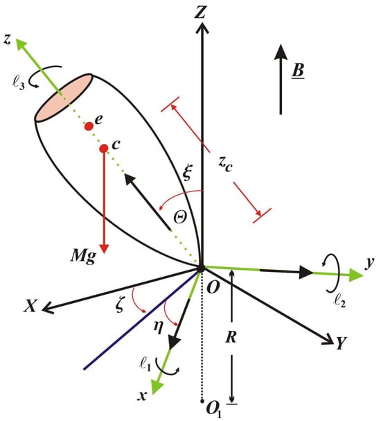
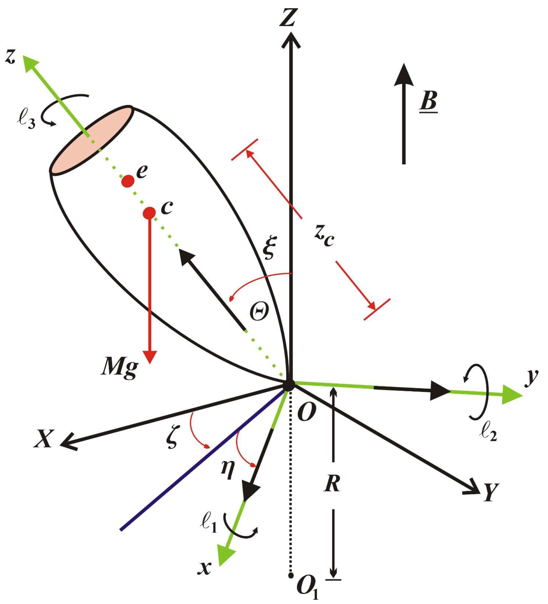
Here, we present the problem to be studied. Our analysis centers on the rotary motion of a symmetric RB (gyrostat) around a stationary point , which is chosen as the origin for two orthogonal frames of reference. The frame is stationary in space, while the frame is stationary to the gyrostat and moves with it; see Figure 1. It should be noted that the gyrostat is symmetric around its dynamic symmetry axis, , along which both the center of mass and the PC for two orthogonal frames of reference are located. In this configuration, the principal inertia tensor and are, respectively, the main inertia’s tensor and the center of mass’s position vector, i.e., . The body rotates under the influence of the EF of strength , produced by a point charge at a distance from the origin that makes an angle with the fixed axis .
Figure 1.
Physical model.
This motion is influenced by an NFF that originates from a source located in the direction opposite to the -axis at a distance from , a uniform EF of strength , generated by a PC that makes an angle with the fixed axis , perturbing moment whose components act along the inertia’s main axes and . Using the law of Lorentz force [23], the resulting force field can be estimated, with as the position vector of charge relative to the center of mass , and as the angular velocity vector. The torque generated, denoted by , has projections on the inertia’s main axes, while the nutation angle is represented by .
The EF considered in this study is modeled as originating from a point charge located along the dynamic symmetry axis. This assumption is both physically sound and practically important for several reasons:
- A point charge produces a standard Coulomb field, offering the simplest analytical representation of a conservative central force that complements an NFF already considered. This symmetry in the modeling framework enables a direct and meaningful comparison between the effects of the two inverse-square fields on the rotational dynamics.
- In space environments, differential surface charging can produce localized high-potential regions on spacecraft structures, which can be effectively modeled as point charges for attitude dynamics analyses.
- This modeling approach also captures interactions with specific onboard components, such as biased instruments or thrusters, as well as with external field sources located at a distance.
- The overarching objective of this work is to examine the nonlinear coupling and stability behavior resulting from the combined action of multiple force and torque types. Employing a simplified but well-structured field model yields tractable and insightful analytical solutions.
To derive the governing EOMs, the fundamental equation of angular momentum [2] is used:
where
In this context, stands for the angular momentum, indicates the resulted moment from the external forces about , and the dot notation denotes differentiation regarding time. The symbol expresses the body’s mass, refers to gravitational acceleration, while is a unit vector pointing along the -axis relative to the inertia’s main axes; is used for the self-rotation’s angle.
Additionally, the angular velocity can be represented through its components as functions of the Euler angles [2].
where and are the nutation and precession angles, respectively.
Therefore, the governing EOMs in the body-fixed coordinate system are as follows [2].
where corresponds to the restoring moment generated by the gyrostatic weight and an NFF, defined as
In this context, represents the distance between the rigid body’s center of mass and the fixed point , represents the gravitational constant associated with the attracting center .
Reviewing Equation (3), one finds that setting and removing an NFF yields the governing EOMs for Lagrange’s case. Additionally, the models in [1] and [17,18] can be reproduced by choosing .
One may, without affecting generality, assume that the gyrostat starts with a small angular velocity close to its dynamic symmetry axis, that the first and second components of PM are less than the restoring moment, and that the third component is of a similar order as . Mathematically, these conditions may be formulated as below.
To meet our goal of utilizing the AM to obtain the relevant averaged system from the governing equations, Equation (3) must be supplemented with an LP . The conditions specified in (5) permit an LP to be inserted as follows.
It is assumed that the new variables and functions and , together with the variables and constants and , are of order unity (i.e., bounded as ). This work is principally concerned with obtaining AS for the original system (3) by means of the AM [9], under the specified conditions in (5) and relations in (6), over a timescale proportional to .
3. Methodology Used
Obtaining AS for the rotation of a charged RB under an NFF and the GM using an LP in view of the AM is critically important for several interconnected reasons:
It is known that the full EOM (modified Euler’s equations, including gravitational, electromagnetic, and gyrostatic torques) is highly nonlinear and coupled. Exact analytical solutions are generally impossible to find. The AM (a form of perturbation theory) allows us to systematically simplify these complex equations by identifying dominant effects (associated with an LP, e.g., low spin rate, strong gravitational field at proximity, or small internal angular momentum from gyrostats) and treating other influences as definite perturbations. This makes the problem mathematically manageable.
The method helps distinguish between primary, slow-scale motions (often related to an LP) and secondary, slower-scale perturbations or secular drifts, which is crucial for understanding the fundamental behavior of the system.
It reveals which forces or moments have the most significant impact on different aspects of the motion (e.g., precession, nutation, secular drift of the spin axis). For instance, a large GM might dominate short-term stability, while smaller Newtonian or electromagnetic torques cause long-term precession.
ASs often led to simplified models that are easier to analyze for stability. Accurate and efficient prediction of motion is essential for applications like spacecraft attitude control, navigation, or robotics. ASs can provide these predictions in real time or near real time.
When designing systems or analyzing celestial body dynamics, engineers and scientists often need to explore a wide range of parameters. AS make extensive parametric studies feasible. Simplified models derived from AS are often the basis for designing feedback control laws for attitude stabilization and maneuvering of spacecraft or other spinning devices. These solutions allow for the prediction of the body’s orientation and angular velocity over time. Understanding the influence of different parameters (charge, mass distribution, gyrostat speed) through the AS helps in optimizing the design for desired performance characteristics.
Based on the above analysis of the method used, it can be stated that the objective of this section is to derive the averaging system corresponding to the original system (3). The AM is used to achieve this aim. This involves substituting expressions from (6) into the governing system (3) and then neglecting terms of order from both sides to obtain a more tractable system in the form,
To derive the desired solutions, the zero-order approximation is taken as the initial approximation, i.e., when . Accordingly, the solutions to the last four equations of the previous system have the following form.
where and denote the constants obtained through integration, matching the variables’ values at the commencement of motion.
By applying Equation (8) alongside the remaining equations from (7) at , and then differentiating the resulting two equations, the following nonlinear system with two degrees of freedom is obtained:
And integrating this system yields
where
Here, , and represent the related values of the variables and at , respectively. Furthermore, signifies the generating system’s oscillation phase. The variables and , being osculating variables of the van der Pol type, are used in place of those specified in Equation (6). Further investigation of system (7) indicates that it exhibits nonlinearity, enabling us to establish a new variable as defined below.
At , Equations (8) and (10) enable the determination of general solutions for system (7). Variables and may be reformulated in an equivalent form by eliminating constants from Equation (10), as follows.
Hence, one can express and as follows.
Considering system (7) at alongside (12), and after understanding the importance of the utilized variables, one replaces and in (7) and (11) with and as new variables. By performing various algebraic operations and based on Equation (13), the subsequent system can be obtained in the form
in which
Analysis of system (14) indicates the presence of slow and fast variables, represented by and , respectively. This system clearly generalizes those found in references [17,18] under the condition , where the PM is independent of the variable , and it also relates to the system described in [1] when equals zero. The dependence of on the fast variable creates complications when attempting to apply the AM to the nonlinear system (14). Consequently, the more tractable case is considered, where is a function of the slow time variable instead. As exhibits periodicity in with a period of , it follows from Equation (10) that these functions are also periodic in and with identical periodicity. System (14) evidently possesses the frequencies and , which are associated with the phases and , respectively. The axial angular velocity (AAV) , the of the GM, and the nutation angle directly influence these frequencies. In the process of averaging system (14), two critical situations must be considered: the non-resonance scenario, which occurs when frequencies lack commensurability (i.e., represent an irrational number), and the resonance scenario, which arises when frequencies exhibit commensurability (i.e., constitute prime natural numbers). For the non-resonant scenario, one can establish the first-approximation asymptotic averaged system by performing independent averaging operations on the right-hand sides of Equation (14) regarding the fast variables and . Upon altering the argument and eliminating the variable from the sides of Equation (14), the following is yielded.
In this context, prime symbols indicate differentiation with respect to , the slow time variable, and , where
Note that both the restoring moment and its derivatives regarding are functions of . In the following section, several applications concerning the gyrostatic perturbed movement will be explored.
In essence, the AM provides a powerful toolkit to unlock an understanding of otherwise intractable problems. It transforms a complex, unsolvable system into a hierarchy of simpler, solvable problems, yielding valuable insights and practical tools for analysis, design, and prediction.
4. Applications
This section aims to introduce novel outcomes for applications formerly addressed in [1] and [17,18], with emphasis on the gyrostat’s rotational motion, utilizing the aforementioned AM procedure.
4.1. Case Study: Linear Dissipative Moment
This section examines the perturbed rotational motion of an RB, where the components of the PM are expressed in terms of the slow time parameter . As an important practical example, the case of linear dissipative moments is considered according to Equation (6). For this case, the projections of the PM are expressed in the following forms.
where and are body-dependent constants.
Following the approach outlined above, Equation (17) is substituted into Equation (15). Through subsequent mathematical manipulations, the solution to the averaged system (15) is obtained to a first-order approximation as
Analysis of equation system (18) yields several important findings. The nutation angle preserves its initial value throughout the evolution, while the AAV demonstrates exponential decay characteristic of stable motion. The slow variables and undergo exponential attenuation determined by the parameters or . Concurrently, the precession angle exhibits monotonic growth influenced by the coefficient, with the corresponding mathematical series maintaining convergence.
Substituting and from Equation (18) into Equations (6) and (12) yields
It is clear from Equation (19) that and are expressed in terms of and , and they exponentially decrease, which indicates that their behavior is stable. Additionally, it should be noted that and have a significant relationship with and , respectively. Furthermore, the expression for increases over time.
From various perspectives, one may derive several limited scenarios, such as in [18] when , in [1] when , and in [31] when , together with instances where is a function of only one angular velocity component.
4.2. Case Study: Angular Velocity Component Control
This section examines the regular precession of a gyrostat in its deactivated state. Small control moments of the following form are considered.
Obviously, these expressions represent the most time-efficient reduction of the equatorial projection of angular velocity [32], corresponding to a regular precession motion. Based on Equations (6), (12) and (20), it yields
Applying Equations (15) and (21), and integrating the resulting expressions, yields the following result.
A closer examination of Equation (20) reveals that the angle remains stationary, equal to its initial value. Additionally, the AAV exhibits an increasing trend, positively influenced by its initial value , as well as by the values of certain parameters and the slow variable . As in the first scenario, the evolution of the system depends on four constants, denoted by along with . Finally, the precession angle increases monotonically with time , whose involves a convergent series.
It follows from the previous analysis that and can be expressed by substituting Equation (20) into Equations (6) and (12), in the forms
Several useful conclusions may be drawn from Equation (23). The behavior of and exhibit periodic behavior, indicating a stable dynamic response. Furthermore, both components interact favorably with the gyrostatic torques and as evident from Equation (23). Additionally, the variable shows a beneficial interaction with .
4.3. Case Study: A Dynamically Symmetric Rigid Body’s (RB’s) Entry into the Atmosphere
This subsection explores the situation where the restoring moment can be represented as
with and as constant coefficients, unrestricted in sign. These cases occur in the analysis of uncontrolled 3-D motion of an RB in the atmosphere [33].
Upon substituting Equations (21) and (24) into Equation (15), integrating the resulting equations, and applying Equations (6) and (12), the expressions for argument , precession angle , and are obtained as presented below.
where
It is evident from Equation (25) that increases over time. The expressions and exhibit periodic behavior within the given time interval, indicating that and remain stable.
4.4. Case Study: Evaluation of Motion Affected by a Small Constant Moment
This section is dedicated to analyzing the beneficial effects of a small constant moment on the motion of an RB within the framework of Lagrange’s case. In particular, the body’s response to a small constant moment applied along its axis of dynamic symmetry is investigated. Accordingly, the components of the PM are described as [17]
For the non-resonant scenario, the averaged system given in Equation (15), represented in terms of the variables and , is expressed as follows.
Integration of and yields
where and are constants of integration, with representing the initial value of , and indicating that the nutation angle remains constant throughout the motion. Inserting Equation (28) into the -equation of system (27) and integrating leads to
Here, signifies the precession angle’s arbitrary initial value.
Utilizing the expression for from Equation (28), the solutions to the first two equations of system (27) can be written in the form
By applying Equations (6), (12), (28) and (30), the expression for and are
Analysis of Equation (31) reveals that and are formulated in terms of trigonometric functions, the GM projections on the main axes, the PC, and the restoring moment representing both the body’s weight and the Newtonian term. This extends the findings of Akulenko et al. [17], which pertained to a uniform field without applied moments.
For the validation of the solution and its convergence, we can say that the AM used in this study preserves only the leading (zeroth-order) and first-order terms of the asymptotic expansion. This approach is standard and well justified in perturbation theory when the system exhibits a clear separation of time scales [8,9,17]. The decision to truncate the expansion after the first-order term is supported by the following considerations:
- The introduction of the LP assumes that all terms of order and higher are negligible when compared with the retained terms under the weak oscillation condition (Equation (5)). This assumption is fundamental to the method and is validated a posteriori by the consistency and reliability of the resulting solutions.
- The solutions exhibit physically expected behavior: stability, bounded oscillations, and smooth parameter dependence—with no emergence of unphysical singularities or divergences that might indicate truncation failure.
5. Evaluation of the Outcomes
This section aims to examine the outcomes from the previous applications along with their graphical illustrations. To facilitate this analysis, in this study, the following body parameters are considered:
The purpose of the analyses depicted in Figure 2, Figure 3, Figure 4, Figure 5, Figure 6, Figure 7, Figure 8, Figure 9, Figure 10, Figure 11, Figure 12 and Figure 13 is to examine the favorable impact of the GM and the charge on the dynamic motion of the examined body.
Figure 2.
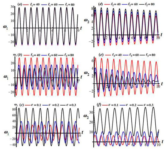
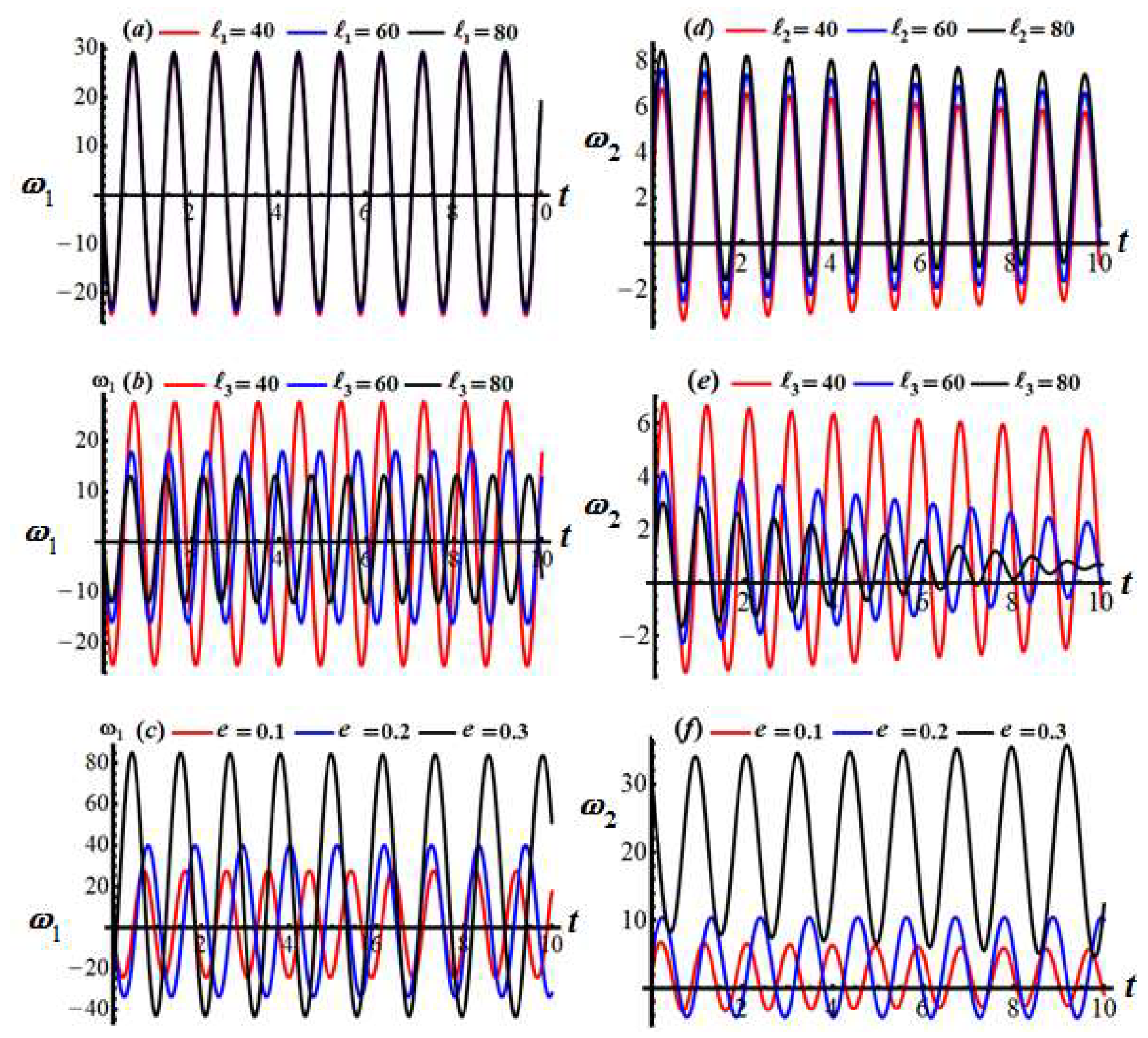
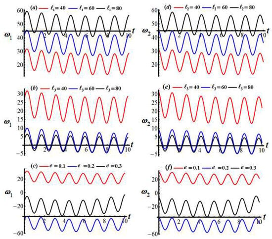
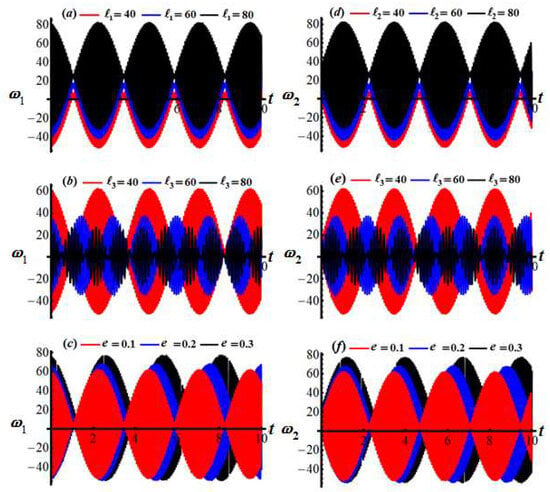
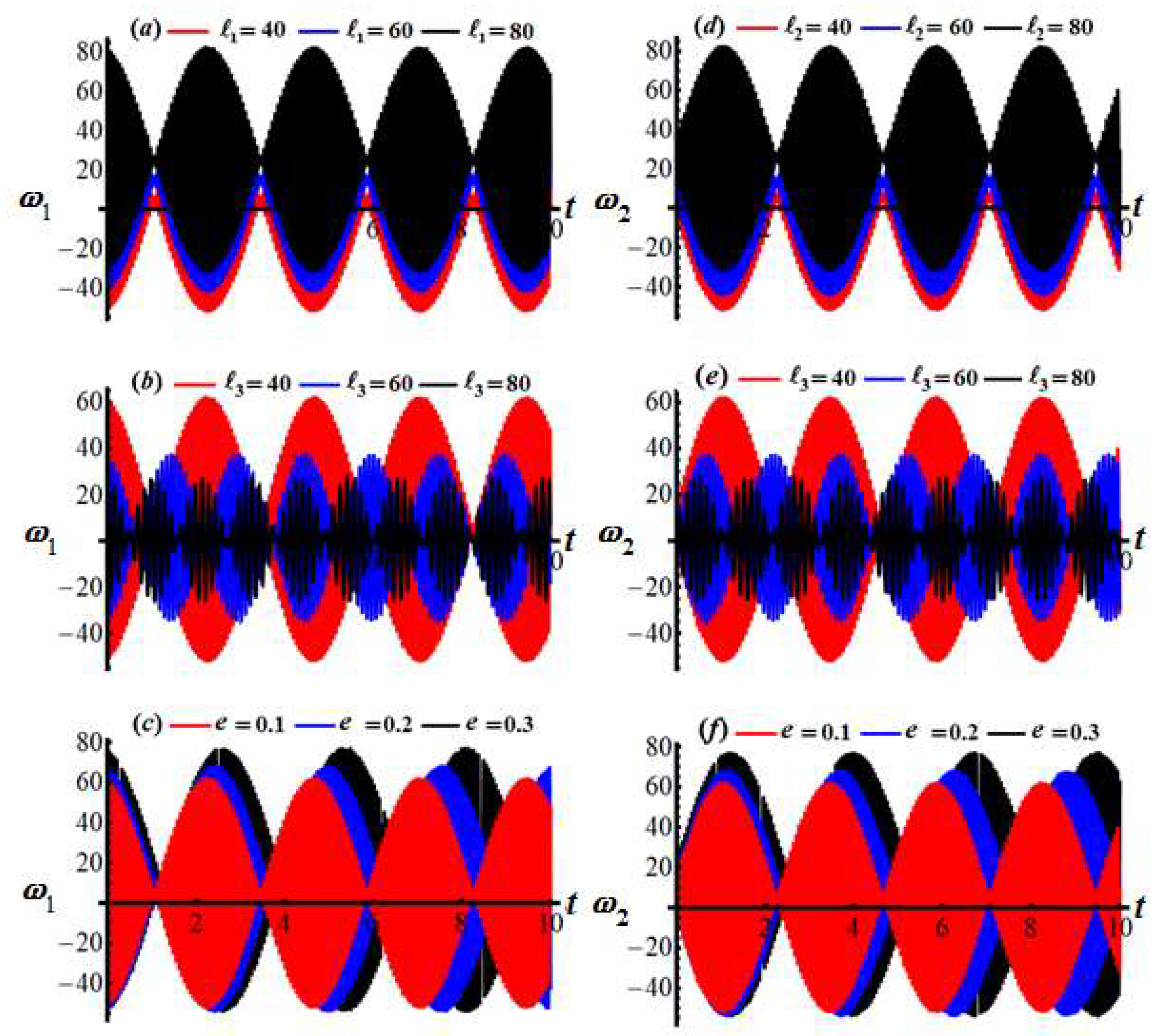
Showing how and vary over time for the first scenario when (a) at and , (b) at and , (c) at and , (d) at and , (e) at and , and (f) at and .
Figure 3.
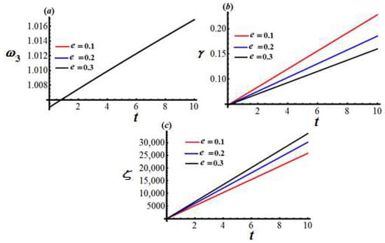
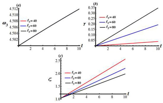
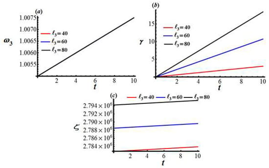
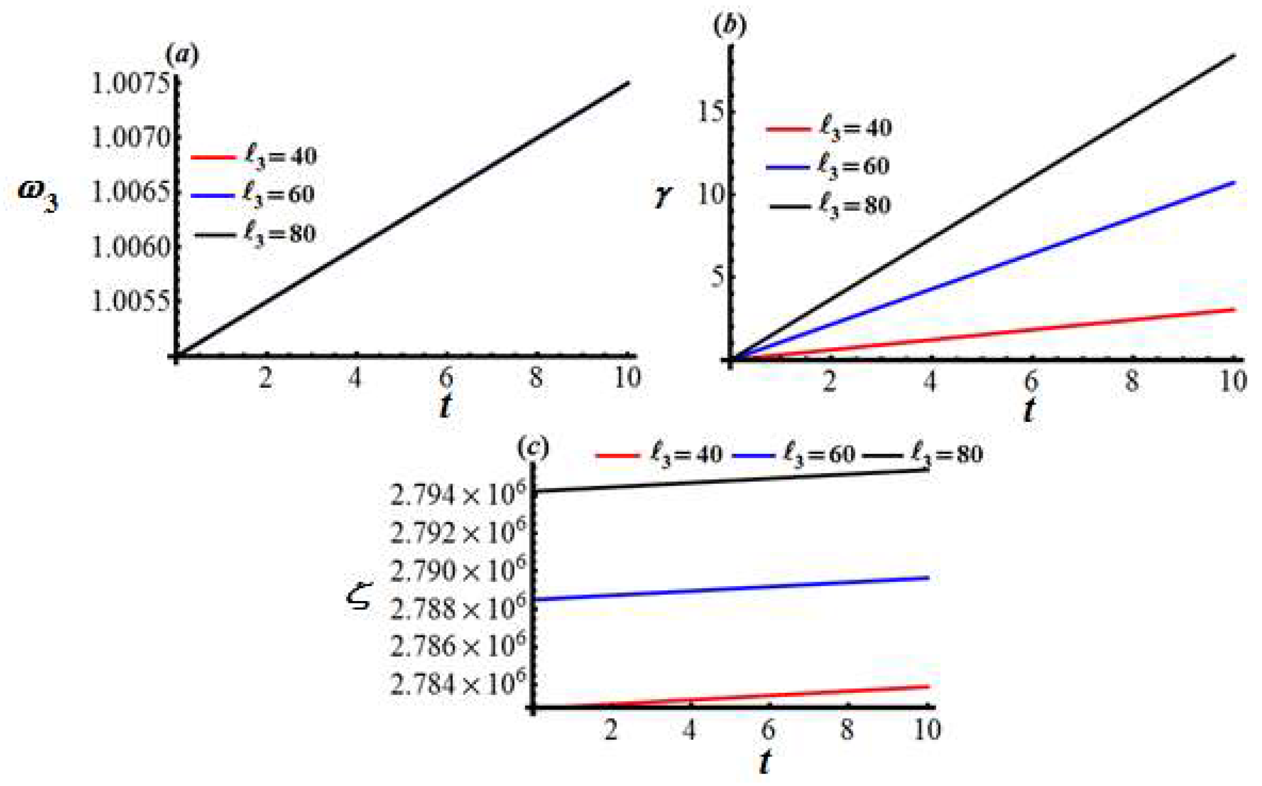
Presenting time-dependent behavior of (a) (b) and (c) for the first scenario at various values of at .
Figure 4.
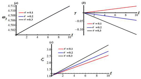
Illustrating time profiles of (a) (b) and (c) for the first scenario at various values of and .
Figure 5.
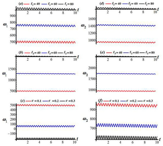
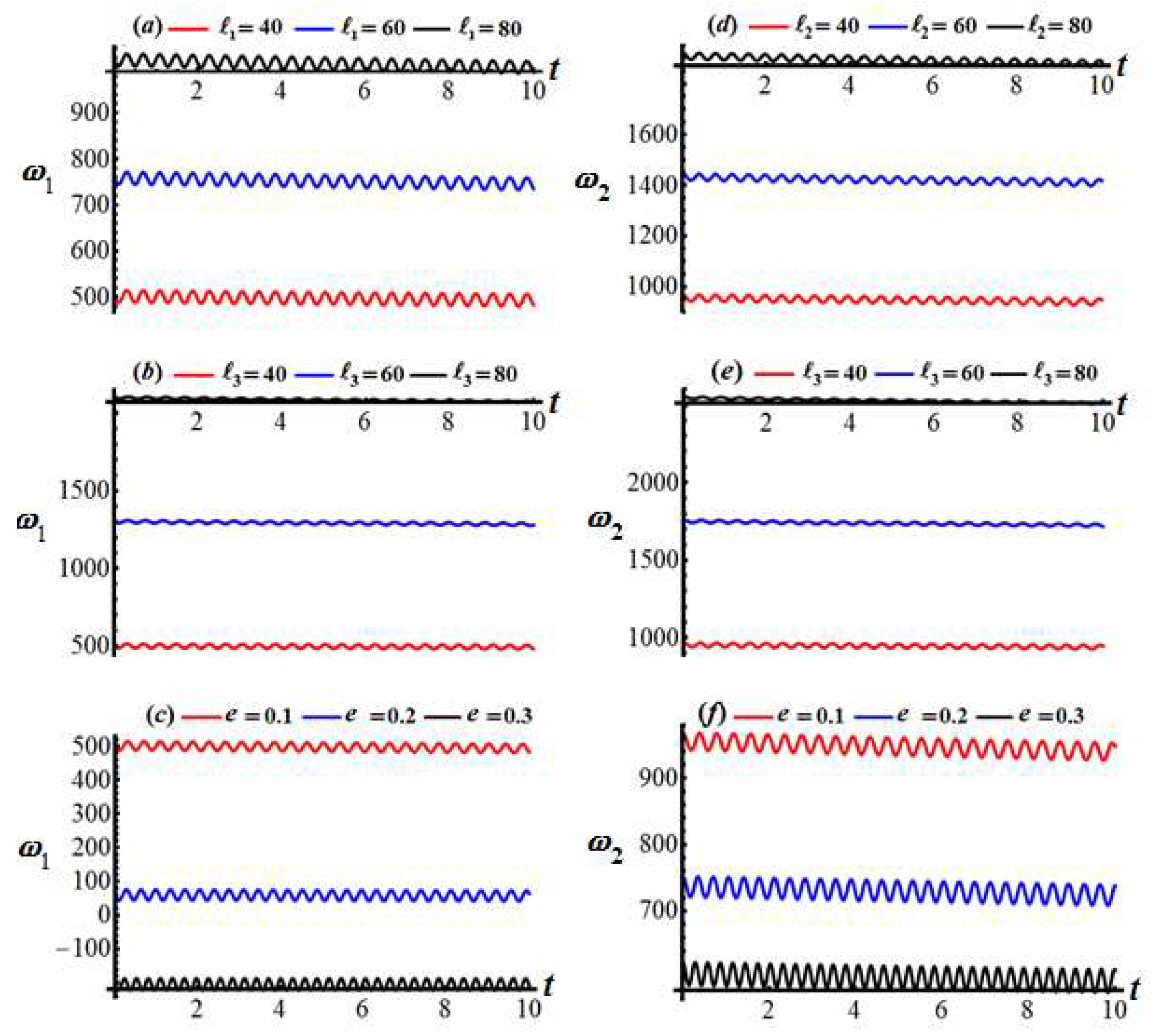
Temporal evolution of and versus time for the GM scenario under different parameter values: (a) variation of. for different values of ; (b) variation of for different values of ; (c) variation of for different values of ; (d) variation of for different values of ; (e) variation of for different values of ; (f) variation of for different values of .
Figure 6.
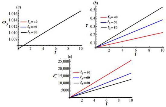
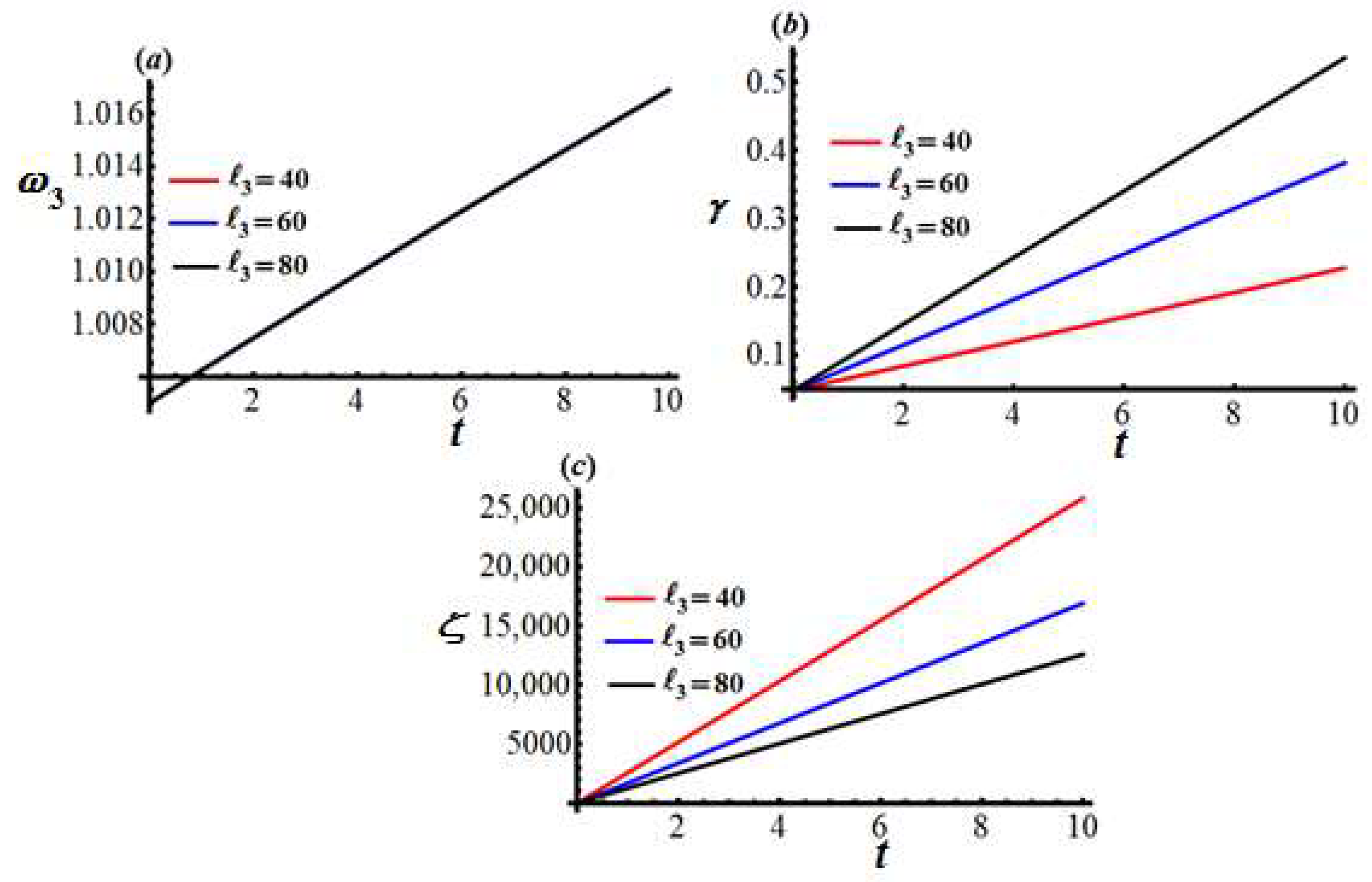
Demonstrating the changes in (a) (b) and (c) ζ over time for the second scenario at distinct values of when the data of Figure 3 are satisfied.
Figure 7.
Depicting the progression of (a) (b) and (c) with time in the second case when has various values and .
Figure 8.
Displaying the influence of the GM on and in the context of axisymmetric body atmospheric entry when the same data in Figure 2 are taken into account (a) influence of the GM on for different values of ; (b) influence of the GM on for different values of ; (c) influence of the GM on for different values of ; (d) influence of the GM on for different values of ; (e) influence of the GM on for different values of ; (f) influence of the GM on for different values of .
Figure 9.
Presenting the time-based variation of (a) (b) γ and (c) ζ in the third instance when has different values, based on the data from Figure 3.
Figure 10.
Highlighting how (a) (b) γ and (c) ζ vary with time for scenario three when has various values at .
Figure 11.
Displaying the influence of the GM on and in the context of axisymmetric body atmospheric entry when the same data presented in Figure 2 are taken into account: (a) Describing the time-dependent wave patterns of and for the small-moment scenario using the same validated data presented in Figure 2: (a) wave patterns of for different values of ; (b) time history of wave response of for different values of ; (c) wave patterns of for different values of ; (d) wave patterns of for different values of ; (e) wave patterns of for different values of ; (f) wave patterns of for different values of .
Figure 12.
Displaying the temporal fluctuations of (a) (b) γ and (c) ζ for the small moment scenario when has different values and the validation of Figure 3 data.
Figure 13.
Presenting the temporal evolution of (a) (b) and (c) over time when has various values at for the small-moment scenario.
Let us break down the interpretation of Figure 2, which shows the time histories of the angular velocity components and under different conditions. The drawn subplots generally depict oscillatory behavior for both and , indicating some form of precessional and/or nutational motion of an RB. The parameters being varied (the GM , and charge ) have distinct effects on the amplitude, frequency, and overall character of these oscillations. Each subplot can be interpreted as follows:
Figure 2a, vs. , varying ( red, blue, black): It is observed that the motion is a clear, regular sinusoidal oscillation. As increases, the amplitude of significantly increases (from approx. ±20 for the indicated values of ). The frequency of oscillation appears to remain nearly constant across the different values of . The period is roughly 0.8 time units. Moreover, the component of the GM (internal angular momentum along the body’s -axis) directly influences the magnitude of the angular velocity component . A larger leads to steady swings in . This suggests that contributes to some extent to the motion around the -axis.
Regarding the Figure 2d, which describes the variation of vs. , varying ( red, blue, black), one can see that the GM component (along the -axis) directly influences the amplitude of . The motion has decaying standing oscillations. As increases, the amplitude of increases (from approx. ±6 for to approx. ±8 for ). The frequency of oscillation appears nearly constant and is the same as in Figure 2a.
Referring to this analysis, the components and primarily affect the amplitude of their respective angular velocity components ( and ) without significantly altering the fundamental frequency of the oscillation in this scenario. This suggests a relatively straightforward precessional/nutational motion where these gyrostatic terms scale the extent of the wobble.
About the Figure 2b, which shows how varies ( red, blue, black): The motion is no longer a simple sinusoid. It exhibits amplitude modulation or a beating phenomenon. For (red), the modulation period is longer (the “envelope” of the wave changes slowly). For (blue), the modulation period is shorter. For (black), the modulation period is even shorter, and the amplitude variation within the envelope is more pronounced. The overall maximum amplitude of also seems to slightly decrease as increases. The component of the GM (along the -axis, often the principal spin axis) introduces a more complex dynamic. The beating pattern suggests an interaction between at least two closely spaced frequencies. Increasing changes the relationship between these frequencies, leading to faster modulation. This could be due to altering stability characteristics or coupling the motions of and in a way that causes periodic energy exchange between different modes of oscillation.
With reference to the Figure 2e— vs. , varying ( red, blue, black): Similar behavior to in Figure 2b is noted but with decay manner. Amplitude modulation is present, and the modulation frequency increases with increasing . For (black), the amplitude of occasionally drops very close to zero. One can interpret this behavior as the effect of on mirroring its effect on . This strongly indicates that is a critical parameter influencing the coupling and energy exchange between the rotational modes associated with and . A large can significantly stabilize or destabilize the motion around the transverse axes, and its variation here is clearly changing the nature of the mutational motion.
According to this assessment, the GM qualitatively changes the motion from simple oscillations to modulated oscillations. It primarily affects the modulation frequency and the envelope of the and oscillations, indicating a more complex interaction and energy transfer within the system’s rotational degrees of freedom.
The following Figure 2c,f, illustrate the effect of varying the charge on the rigid body’s motion. Figure 2c” presents vs., varying ( red, blue, black). The motion is again a regular sinusoidal oscillation. As the charge increases, the amplitude of dramatically increases (from approx. ±20 for , to ±40 for , to approx. ±80 for ). The frequency of oscillation appears to remain nearly constant, like the frequency observed in the Figure 2a,d. The electric charge leads to electromagnetic torques. These torques significantly energize the rotational motion, leading to much larger amplitudes of as the charge increases.
Figure 2f demonstrates how changing the charge affects ( red, blue, black). A regular sinusoidal oscillation is observed. The amplitude of also dramatically increases with increasing (from approx. ±8 for , to ±15 for , to approx. ±30–35 for ). The frequency is nearly constant and matches that in Figure 2c, in which the electromagnetic torques, proportional to the charge , also drive larger oscillations in .
Therefore, one can say that the magnitude of the PC has a profound impact on the amplitude of both and oscillations. Larger charges lead to significantly larger rotational disturbances, likely due to increased electromagnetic torques. The fundamental frequency of these oscillations seems largely unaffected by in this set of simulations, suggesting the charge primarily scales the forcing term.
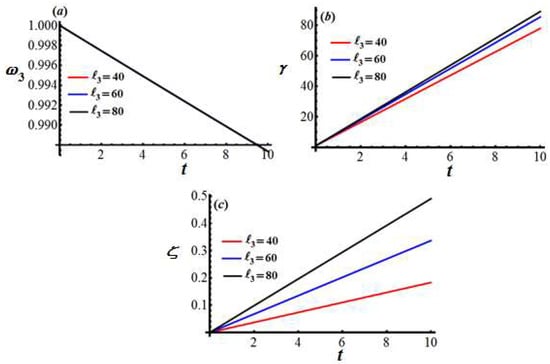
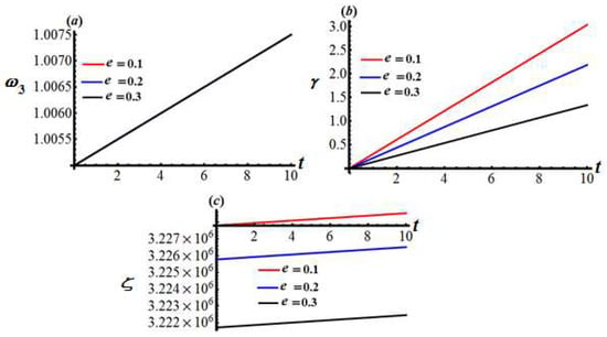
A closer inspection of Figure 3a shows that all three colored curves lie exactly on top of one another. decreases almost imperceptibly: from at to at . The axial spin-rate decay is dictated by a mechanism that does not depend on the GM . That means the spin decay is imposed by a torque that acts about the spin axis itself. According to Figure 3b in the same figure, one can observe that grows strictly linearly with time. The slope order of the black line () is greater than that of the blue one (), and consequently the latter is greater than the red line (). A larger GM increases the nutation rate; physically, the body with the bigger resists changes in spin but more readily reorients its axis, so the tilt accumulates faster. Considering Figure 3c, one observes that also increases linearly, starting from . The slopes scale with exactly as in . Faster nutation produced by the larger GM is accompanied by a faster, prograde precession. Therefore, the results indicate that adjusting the GM barely affects the spin decay but linearly amplifies both the nutation and the (prograde) precession rates.
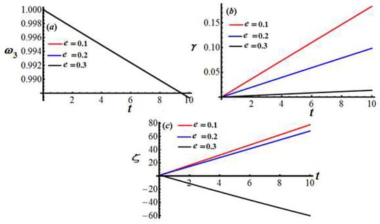
The influence of the magnitude of the PC (where are fixed) on and can be seen in the portions a, b, and c of Figure 4, respectively. As in Figure 4a, curves for are indistinguishable. The same small linear decay is seen in Figure 3a. The axial spin rate is not sensitive, to some extent, to the values of . Whereas again grows linearly, as seen in Figure 4b, now the slope is controlled by : red () has the steepest slope, blue () is milder, and black () is almost flat. Increasing suppresses the tilt motion. The variation of via when shows that increases linearly and positively, just as in Figure 3c. At a higher , the slope changes sign, in which decreases, reaching roughly by as a retrograde precession. A large value of not only slows -growth, but it also reverses the sense of precession. The torque produced by the displaced mass overcomes the gyroscopic tendency for prograde motion.
The aforementioned examination leads one to the conclusion that the spin behavior is essentially parameter-independent: its slope is fixed by the chosen model’s structure, not by either or —it is accelerated by a larger value of the GM . It is decelerated by a larger value of . The behavior of is directly proportional when precession is prograde. It can switch to retrograde once the stabilizing couple created by outweighs gyroscopic coupling. Therefore, to achieve a fast-pointing (quickly re-orienting) rotor, it is required to increase but keep the smaller value of e. If stability with minimal nutation/precession is desired, introduce ; too much, however, will reverse the precession direction.
Below is a thorough interpretation of Figure 5, Figure 6 and Figure 7, focusing on the dynamics of the examined RB for the case of controlling angular velocity.
Figure 5 represents time histories of transverse angular velocities (), in which panels Figure 5a, Figure 5b, Figure 5d, Figure 5e, and Figure 5c, Figure 5f examine the effect of the GM , and the PC , respectively.
To study the influence of and on the behavior of and , Figure 5a,d are plotted. The mean angular velocity increases as increases (40 to 80). The amplitude is small, and the frequency is consistent across all values of . Therefore, increasing raises the bias angular velocity. It increases the gyrostatic coupling influence, leading to larger steady-state transverse rotation.
The mean velocity grows with in Figure 5b, as does similar behavior in Figure 5a. Consistent frequency in oscillations is noticed, indicative of a constant nutation rate. A larger , just like , enhances the momentum about its axis, raising transverse spin.
The good impact of is examined through the drawn curves in parts b and e of Figure 5. The mean level of significantly increases with a larger . This means that the axial spin interacts with transverse components due to cross-coupling, elevating the transverse angular velocities. A similar rise in mean with increasing is observed in panel e. A larger translates to a stronger spin-stabilization effect, which elevates transverse rates due to enhanced cross-coupling.
The effect of various values of the PC is examined in panels c and f of Figure 5. Panel c describes the variation of with . It must be mentioned that a larger creates stronger electromagnetic torque, damping gyrostatic influences, and reducing wobble, whereas panel f describes with varying , in which a larger suppresses the baseline and oscillations. In other words, increasing stabilizes the body against wobble by applying strong electromagnetic counter-torques.
An inspection of panel a of Figure 6 shows the time-dependent behavior of the axial spin when varies. It is noted that there is a linear increase over time, with steeper slopes for a larger . This means that gyroscopic stabilization improves with a larger , effectively translating external torques into increased spin. The variation of with is plotted in panel b, in which there is a linear increase with a steeper slope for a larger , which grows faster as the GM influences it, making the axis more responsive to tilting forces. Regarding the variation of , as seen in panel c, rapid linear growth is noted, with an inverse relationship to the value. In other words, a smaller means a reduced GM, allowing other torques to drive quicker precession.
Based on the curves in Figure 7, one can state that there are linear increases in the behavior of the AAV , and the slope gets steeper with a larger , as indicated in Figure 7a. A greater implies stronger electromagnetic torque, energizing the spin direction. The rate of decreases with a larger , as in Figure 7b, and consequently, the electromagnetic force acts like a stabilizing torque, moderating nutation. According to Figure 7c, the behavior of has a linear form, in which it increases with a larger slope as increases, and stronger electromagnetic control from a higher enhances precessional torque around external fields.
As shown in Figure 6 and Figure 7, the AAV and the angles and increase steadily over time , consistent with the harmonic pattern defined by Equation (22).
Now, the unified physical implications of the second examined case are summarized as follows:
Adjusting the GM and allows fine-tuning of bias rotations and maintains desired transient responses. Larger values increase system responsiveness. Electromagnetic influence acts as a stabilizing force, decreases wobble, and lets one control the overall spin-up and precession dynamics, where increased dramatically boosts precessional rates. Through the interplay of the GM and external electromagnetic torques, the figures characterize the complex stability-regulating mechanism of a spinning charged body.
Figure 8, Figure 9 and Figure 10 illustrate the rotational dynamics of an axisymmetric RB under diverse conditions, including variations in the GM and electromagnetic influences characterized by the PC . The subsequent analysis is structured into three primary sections, corresponding to the insights derived from these figures.
Figure 8 illustrates the variation of the angular velocity components and under the influence of the GM . Figure 8a,d reveal the oscillatory behavior of and as and are varied. Notably, as or increases, the corresponding amplitude of the oscillations grows, while the frequency remains relatively constant. This suggests that larger gyrostatic moments lead to more pronounced rotational dynamics.
Furthermore, Figure 8b,e demonstrate that changes in have a significant impact on the amplitude of and . Specifically, higher values of result in reduced oscillation amplitudes, indicating a stabilizing effect on the body’s rotational motion.
The PC has a notable impact on the oscillations of and , as evident in Figure 8c,f. The variation of yields distinct oscillation patterns for both angular velocity components. Notably, when , exhibits negative values, suggesting a reversal in the direction of rotation or a substantial modification in the rotational dynamics resulting from electromagnetic interactions.
With respect to Figure 9, which illustrates the behavior of the AAV and the angles and , several key observations can be made. Firstly, as shown in Figure 9a, exhibits an almost linear increase with time, displaying a slight dependence on the GM . However, the variation across different values is minimal. Secondly, Figure 9b reveals a direct relationship between and the angle , as increases with , suggesting that the GM around the axis of symmetry influences the precession or nutation angle. Furthermore, Figure 9c demonstrates that increases linearly with time, but with a slope that decreases as increases. This indicates that higher values lead to a more gradual change in , potentially signifying a more stable spatial orientation.
The effect of the PC on the AAV and the angles and is investigated in Figure 10. As depicted in Figure 10a, the increase in is consistent across various values of , suggesting that the PC has a negligible impact on . In contrast, Figure 10b reveals a significant dependence of on . Specifically, for , increases, whereas for higher values of ( and ), decreases, indicating that stronger electromagnetic influences can modify the precession dynamics. Furthermore, Figure 10c shows that increases with time for all values of , but the rate of increase is more pronounced for a larger , implying that enhanced electromagnetic interactions amplify the change in .
Based on the foregoing analysis, it is evident that the rotational dynamics of the axisymmetric body are substantially influenced by both the GM and electromagnetic effects associated with . The GM components significantly impact the oscillatory behavior of the and , with exerting a stabilizing influence. The introduction of e induces variability in the rotational dynamics, affecting the oscillations of and , as well as the evolution of the angles and . Notably, the AAV remains relatively stable, exhibiting minimal sensitivity to , while displaying a slight increase with .
These outcomes imply that the design and control of spacecraft or re-entry vehicles necessitate a comprehensive consideration of both mechanical GM and electromagnetic factors to accurately predict and stabilize their rotational dynamics during atmospheric entry or other operational phases.
An examination of Figure 11 reveals that the time histories of and display periodic oscillations, signifying intricate rotational dynamics that are influenced by both the GM and the PC . The amplitudes and frequencies of these oscillations are sensitive to variations in the aforementioned parameters.
As depicted in Figure 11a,d, increasing and amplifies the oscillations of and , resulting in more pronounced rotational dynamics. Furthermore, Figure 11b,e illustrate that has a significant impact on the oscillations, with higher values leading to a decrease in amplitude and the emergence of higher-frequency components, suggesting a stabilizing effect. Additionally, Figure 11c,f demonstrate that variations in yield distinct oscillation patterns for and , underscoring the influence of electromagnetic forces on the rotational dynamics.
The influence of on is illustrated in Figure 12a, where it is evident that increases nearly linearly with time, exhibiting a slight dependence on . This suggests stable rotational motion around the axis of symmetry. Furthermore, as shown in Figure 12b, the angle increases with , indicating a direct correlation between the GM and the precession or nutation angle. In contrast, Figure 12c reveals that exhibits minimal variation with , implying that has a limited effect on this angle.
From Equations (28) and (29), it is evident that and increase monotonically over time, as highlighted in Figure 12a–c at . Moreover, the impact of rising on the precession angle causes a corresponding increase in its behavior. The notably large magnitude of arises from the second term of Equation (29), where is relatively small (0.001). Examining the solutions of Equation (31) reveals that increases gradually with time, as shown in Figure 12b and Figure 13b. In light of all the cases analyzed, therefore, the motion of this body remains stable and is not subject to any chaotic dynamics.
The impact of different values of on and the angles and is illustrated in Figure 13. As depicted in Figure 13a, the increase in is consistent across various values, suggesting that has a negligible influence on . Moreover, Figure 13b reveals that increases with time for all values, but with a higher rate of increase for lower , indicating that stronger electromagnetic influences modify the precession dynamics. Additionally, Figure 13c shows that exhibits minimal variation with , implying that electromagnetic effects have a limited impact on this angle.
Physical Analysis of the Outcomes
The analysis presented in this subsection is as follows: The oscillation amplitude of both and increases when the components and of the GM are increased. This indicates that the body exhibits greater “wobbling” (nutation) and strongly resists orientation changes. This effect is like the widening of oscillatory motion that occurs in heavy gyroscopes when the internal moment is increased. In contrast, the component produces an interference or “beating” pattern in the transverse angular velocities, which is similar to a recurring energy exchange between nutation and precession motions. By modifying to make the beating frequency fast enough to not influence system stability, these phenomena can be successfully used in the design of vibration dampening systems for satellites. We noticed that increasing the electric charge considerably increases the amplitude of and up to four times because the charge in a magnetic field is expressed as an energy pump that injects energy into the transverse motion. This has important practical ramifications: spacecraft exposed to charge buildup from surrounding plasma may suddenly become unstable, necessitating the creation of effective charge neutralization technology.
Regarding the temporal behavior of the angles and velocities, the body rotates about its vertical axis at a nearly constant rate due to the monotonic increase in the precession angle and the phase , whereas the axial angular velocity either increases or decreases exponentially depending on the direction of . This is consistent with basic physics: rotation accelerates when the GM is in the direction of rotation; it slows down when it is in the opposite direction. The precession angle with time in the atmospheric entry case examined in Section 4.3 is noted. This is consistent with the known behavior of long projectiles, like rockets, when they enter a dense atmosphere, where the precession angle increases and may result in aerodynamic instability.
In closing, engineers as well as designers can determine the useful suggestions to consider, in which should be made larger than the charge effect to maintain precession stability; and can be increased while accepting larger oscillations to increase system responsiveness; and it is advised to use a small charge and a large GM to minimize wobble. As a result, the findings offer both a mathematical explanation and direct, useful advice that can be applied to control applications for rotating rigid structures like satellites, aircraft, and submarines.
We are currently providing a comparison of the current study with the previous study, which is described in Table 1. The functions and are proposed to describe the admissible domains of the system solutions to make this comparison easier. In particular, the domain of the axial angular velocity solution is described by the function , while the equivalent domain of the Euler angles derived from the averaged system is represented by the function . These functions can be represented mathematically in the generic form , . The evolution of the acceptable solution domains under various asymptotic bounds of the perturbation parameter employed in the analytical formulation is described by these functions.
Table 1.
The differences between the previous works and the work considered.
A quantitative validation of the obtained approximate solutions is carried out by comparing them with the numerical solutions of the full nonlinear system using direct numerical integration. The maximum and mean absolute and relative errors for the main dynamical variables are presented in Table 2.
Table 2.
Error analysis between approximate and numerical solutions.
The results demonstrate that the errors remain sufficiently small over the considered time interval, confirming the high accuracy of the averaging method. This quantitative agreement supports the validity of the asymptotic solutions and provides a rigorous basis for the stability conclusions drawn in this study.
6. Conclusions
This work focuses on the symmetric attitude movement of an RB about one of its main inertia axes under the influence of an NFF, an electromagnetic field, and several torque contributions, specifically perturbing and gyrostatic torques. By including an LP for a body starting with small angular velocity away from the axis of symmetry and by assuming that PMs are smaller than the restoring moment, the original system of motion can be averaged and used to analyze various scenarios: dissipative torques, managing angular velocity components, axial motion during entry into an atmosphere, and the impact of small constant moments. The resultant figures verify that the derived solutions remain stable, emphasizing the constructive impact of external influences on the motion. The GM , particularly , plays a pivotal role in stabilizing the body’s rotational motion. A thorough understanding of these effects is essential for the design of effective control systems. Furthermore, the PC has a profound impact on rotational dynamics, particularly on the precession and nutation angles. This is of paramount importance for spacecraft operating in environments characterized by significant electromagnetic influences. To ensure stable and predictable rotational dynamics, it is imperative to account for the intricate interplay between mechanical and electromagnetic forces in the design of spacecraft or re-entry vehicles. These insights highlight the importance of a comprehensive understanding of the rotational dynamics of axisymmetric bodies under various mechanical and electromagnetic conditions.
Author Contributions
Conceptualization, T.S.A., R.K.H., and H.F.E.-K.; methodology, T.S.A., M.A.I., and H.F.E.-K.; software, T.S.A. and M.A.I.; validation, T.S.A., M.A.I., and A.I.I.; formal analysis, T.S.A., A.I.I., and H.F.E.-K.; investigation, T.S.A. and R.K.H.; resources, T.S.A. and M.A.I.; data curation, T.S.A., R.K.H., and A.I.I.; writing—original draft preparation, H.F.E.-K.; writing—review and editing, T.S.A. and R.K.H.; visualization, H.F.E.-K. All authors have read and agreed to the published version of the manuscript.
Funding
This work was supported and funded by the Deanship of Scientific Research at Imam Mohammad Ibn Saud Islamic University (IMSIU) (grant number IMSIU-DDRSP2602).
Data Availability Statement
Since no datasets were accumulated or handled throughout the existing work, data sharing is not appropriate for this study.
Conflicts of Interest
The authors declare no conflicts of interest.
Abbreviations
The following abbreviations are used in this manuscript:
| AAV | Axial Angular Velocity |
| AM | Averaging Method |
| AS | Approximate Solutions |
| ASP | Approach of Small Parameter |
| DE | Differential Equation |
| EF | Electromagnetic Field |
| EOMs | Equations of Motion |
| GM | Gyrostatic Moment |
| LP | Large Parameter |
| NFF | Newtonian Force Field |
| PC | Point Charge |
References
- Amer, T.S.; Abady, I.M. On the motion of a gyro in the presence of a Newtonian force field and applied moments. Math. Mech. Solids 2017, 23, 1263–1273. [Google Scholar] [CrossRef] [Scilit]
- Leimanis, E. The General Problem of the Motion of Coupled Rigid Bodies About a Fixed Point; Springer: New York, NY, USA, 1965. [Google Scholar] [CrossRef] [Scilit]
- Amer, W.S. Modelling and analyzing the rotatory motion of a symmetric gyrostat subjected to a Newtonian and magnetic fields. Results Phys. 2021, 24, 104102. [Google Scholar] [CrossRef] [Scilit]
- Yehia, H. New integrable cases in the dynamics of rigid bodies. Mech. Res. Commun. 1986, 13, 169–172. [Google Scholar] [CrossRef] [Scilit]
- Yehia, H.M. New generalizations of the integrable problems in rigid body dynamics. J. Phys. A Math. Gen. 1997, 30, 7269–7275. [Google Scholar] [CrossRef] [Scilit]
- Yehia, H.M.; Elmandouh, A.A. New conditional integrable cases of motion of a rigid body with Kovalevskaya’s configuration. J. Phys. A Math. Theor. 2010, 44, 012001. [Google Scholar] [CrossRef] [Scilit]
- Elmandouh, A.A. New integrable problems in rigid body dynamics with quartic integrals. Acta Mech. 2015, 226, 2461–2472. [Google Scholar] [CrossRef] [Scilit]
- Elmandouh, A.A. New integrable problems in a rigid body dynamics with cubic integral in velocities. Results Phys. 2017, 8, 559–568. [Google Scholar] [CrossRef] [Scilit]
- Nayfeh, A.H. Perturbation Methods; John Wiley & Sons: Hoboken, NJ, USA, 1978; Volume 8, pp. 417–418. [Google Scholar] [CrossRef] [Scilit]
- Galdi, G.; Mazzone, G.; Mohebbi, M. On the motion of a liquid-filled heavy body around a fixed point. Q. Appl. Math. 2017, 76, 113–145. [Google Scholar] [CrossRef] [Scilit]
- Amer, T.S.; Alanazy, A.; Elneklawy, A.H.; Amer, W.S.; El-Kafly, H.F. Asymptotic solutions for the 3D motion of asymmetric charged gyrostatic satellite using poincaré small parameter technique. Aerosp. Sci. Technol. 2026, 168, 110764. [Google Scholar] [CrossRef] [Scilit]
- Arkhangel’skii, I.A. On the motion about a fixed point of a fast spinning heavy solid. J. Appl. Math. Mech. 1963, 27, 1314–1333. [Google Scholar] [CrossRef] [Scilit]
- Farag, A.M. Analysis of the rotational motion of a solid body in the presence of external moments. J. Vib. Eng. Technol. 2023, 12, 757–771. [Google Scholar] [CrossRef] [Scilit]
- Hussein, R.K.; Ibrahem, M.A.; Amer, T.S.; Elneklawy, A.H. Rotational Dynamics and Stability of Gyrostatic Systems with Prescribed Internal Mass Motion: Asymptotic Methods and Spacecraft Attitude Control. Mathematics 2026, 14, 1463. [Google Scholar] [CrossRef] [Scilit]
- Vera, J.A.; Vigueras, A. Hamiltonian dynamics of a gyrostat in the N-Body problem: Relative equilibria. Celest. Mech. Dyn. Astron. 2006, 94, 289–315. [Google Scholar] [CrossRef] [Scilit]
- Hussein, A.M. On the motion of a magnetized rigid body. Acta Mech. 2017, 228, 4017–4023. [Google Scholar] [CrossRef] [Scilit]
- Akulenko, L.D.; Zinkevich, Y.S.; Kozachenko, T.A.; Leshchenko, D.D. The evolution of the motions of a rigid body close to the Lagrange case under the action of an unsteady torque. J. Appl. Math. Mech. 2017, 81, 79–84. [Google Scholar] [CrossRef] [Scilit]
- Akulenko, L.D.; Leshchenko, D.D.; Kozachenko, T.A. Evolution of Rotations of a Rigid Body Under the Action of Restoring and Control Moments. In Proceedings of the ASME 2005 International Design Engineering Technical Conferences and Computers and Information in Engineering Conference, Long Beach, CA, USA, 24–28 September 2005; pp. 737–741. [Google Scholar] [CrossRef] [Scilit]
- Llibre, J.; Nabavi, A.; Mousavi, M. Limit Cycles Bifurcating from a Family of Reversible Quadratic Centers via Averaging Theory. Int. J. Bifurc. Chaos 2020, 30, 2050051. [Google Scholar] [CrossRef] [Scilit]
- Tsiotras, P.; Longuski, J.M. A complex analytic solution for the attitude motion of a near-symmetric rigid body under body-fixed torques. Celest. Mech. Dyn. Astron. 1991, 51, 281–301. [Google Scholar] [CrossRef] [Scilit]
- Panayotounakos, D.E.; Sotiropoulos, N. Exact analytic solutions of unsolvable classes of first- and second-order nonlinear ODEs (Part II: Emden–Fowler and relative equations). Appl. Math. Lett. 2005, 18, 367–374. [Google Scholar] [CrossRef] [Scilit]
- Panayotounakos, D.E.; Rizou, I.; Theotokoglou, E.E. A new mathematical construction of the general nonlinear ODEs of motion in rigid body dynamics (Euler’s equations). Appl. Math. Comput. 2011, 217, 8534–8542. [Google Scholar] [CrossRef] [Scilit]
- Buck, J.A.; Hayt, W.H. Engineering Electromagnetics; McGraw-Hill Education: Columbus, OH, USA, 2011; ISBN 9780073380667. [Google Scholar]
- Panayotounakos, D.E.; Theocaris, P.S. On the Decoupling and the Solutions of the Euler Dynamic Equations Governing the Motion of a Gyroscope. ZAMM—J. Appl. Math. Mech./Z. Für Angew. Math. Und Mech. 1990, 70, 489–500. [Google Scholar] [CrossRef] [Scilit]
- Amer, T.S.; Hussein, R.K.; Ivanova, E.A.; Elneklawy, A.H. Semi-analytic solutions for finite-rotation attitude dynamics of gyrostatic rigid bodies. Eur. J. Mech.—A/Solids 2026, 119, 106131. [Google Scholar] [CrossRef] [Scilit]
- Fares, M.E.; El-Gohary, A. Stochastic stabilization of the rotational motion of a rigid body using rotors. Int. J. Non-Linear Mech. 2001, 36, 565–570. [Google Scholar] [CrossRef] [Scilit]
- El-Gohary, A. Optimal stabilization of an equilibrium position of a rigid body using rotors system with friction forces. Chaos Solitons Fractals 2004, 23, 1585–1597. [Google Scholar] [CrossRef] [Scilit]
- Leshchenko, D.; Ershkov, S.; Kozachenko, T. Perturbed rotational motions of a nearly dynamically spherical rigid body with cavity containing a viscous fluid subject to constant body fixed torques. Int. J. Non-Linear Mech. 2022, 148, 104284. [Google Scholar] [CrossRef] [Scilit]
- Disser, K.; Galdi, G.P.; Mazzone, G.; Zunino, P. Inertial Motions of a Rigid Body with a Cavity Filled with a Viscous Liquid. Arch. Ration. Mech. Anal. 2016, 221, 487–526. [Google Scholar] [CrossRef] [Scilit]
- Tsiotras, P.; Longuski, J.M. New kinematic relations for the large angle problem in rigid body attitude dynamics. Acta Astronaut. 1994, 32, 181–190. [Google Scholar] [CrossRef] [Scilit]
- Rozenblat, G.M.; Reshmin, S.A. On Optimal Rigid Body Rotation with Application of Internal Forces. Mech. Solids 2023, 58, 2779–2791. [Google Scholar] [CrossRef] [Scilit]
- Akulenko, L.D. Problems and Methods of Optimal Control; Springer: Dordrecht, The Netherlands, 1994. [Google Scholar] [CrossRef] [Scilit]
- Leshchenko, D.; Ershkov, S.; Kozachenko, T. Evolution of a heavy rigid body rotation under the action of unsteady restoring and perturbation torques. Nonlinear Dyn. 2021, 103, 1517–1528. [Google Scholar] [CrossRef] [Scilit]

Disclaimer/Publisher’s Note: The statements, opinions and data contained in all publications are solely those of the individual author(s) and contributor(s) and not of MDPI and/or the editor(s). MDPI and/or the editor(s) disclaim responsibility for any injury to people or property resulting from any ideas, methods, instructions or products referred to in the content. |
© 2026 by the authors. Licensee MDPI, Basel, Switzerland. This article is an open access article distributed under the terms and conditions of the Creative Commons Attribution (CC BY) license.