Implementing Sensor Signal Fusion for Accurate Positioning of Micro-Robotic Systems

Abstract

Modern scanning microscopes and robotic scanning systems increasingly use visual recognition and machine learning technologies to extract complex data from acquired images. This study examined sensor data fusion in optical imaging to detect and control the deviation of the position of the tool during various micro-manipulations for biologic and microscale engineering. The sensor data fusion study was performed using a scanning micro-robotic system with an integrated optical microscope and a vision sensor providing an image of the object’s bottom. The bottom vision sensor is a typical complementary metal–oxide–semiconductor sensor that is used to observe micrometer-sized semi-transparent objects. The challenge for sensor fusion in such a study is not only data fusion, but also the trajectory deviation inherent in directing the manipulator in the X and Y directions according to the selected trajectory. The data fusion method was applied to estimate deviations from the given trajectory of the scanning microscope. The unique novelty of this work is that an additional vision sensor is used to increase the accuracy of positioning determination of a scanning micro-robotic system, placed under the semi-transparent object, using the fusion of the obtained data, thus additionally controlling the objective deviations. By testing several known data fusion methods, a unique solution was achieved. The proposed sensor fusion method achieved a positioning accuracy of less than 0.5 μm at speeds up to 5 mm/s. Experimental results demonstrate that the system maintains high stability. This quantitative performance proves the system’s suitability for high-precision biological micro-manipulation, where mechanical drift was previously a limiting factor.

1. Introduction

The emergence of miniaturized technologies in the last century has raised various issues of technological convergence, especially with the introduction of micro-manipulation methods, which were driven by enormous advances in fundamental physics, as well as in sensing and actuation techniques, and precision instrumentation. Micro-manipulation techniques have, in turn, enabled advances in many scientific disciplines, especially in the life sciences and their biomedical applications. In a wide variety of scientific and industrial fields, accurate maintenance and high-precision positioning at the micrometric scale are basic requirements. Such domains include advanced manufacturing, robotics, and high-resolution microscopy. Despite significant advances in electromechanical systems and control techniques, fundamental limitations remain that make it difficult to achieve truly precise and repeatable micrometric movements. These limitations are primarily due to a complex cooperation of mechanical inaccuracies and dynamic environmental factors, which together degrade the precision of the entire positioning system [1,2,3]. These difficulties reveal an essential aspect of high-precision positioning in that environmental factors are not just disturbances from the outside world, but even active layers that create and amplify mechanical inaccuracies. For example, temperature changes cause thermal expansion and, as a result, uneven forces within parts of the device [4]. Vibrations cause unwanted mechanical movements, leading to complex errors and instability that directly produce mechanical errors [5]. High-definition optical cameras and hardware/software configuration allow for removing image distortion in real-time displacement measurement [6]. However, high-precision measurements are not simply about achieving mechanical perfection or eliminating environmental noise. This task requires a deep understanding of the problem. Moreover, it often comes at the cost of actively compensating for this with real-time adjustments rather than relying on passive mechanisms [7]. Microscopy-based surface measurements are employed to investigate surface textures. The axial resolution and influence of instrument-generated noise depend on the magnification. Different modes of illumination can overcome technical limitations. Thus, sensor fusion techniques (SF) can improve the accuracy of surface measurements [8,9]. Three-dimensional microscopy has become an essential tool for the study of samples in various fields, from scientific research to industrial applications, from live tissue engineering to single-cell process monitoring. However, the imperfect movement of the scanner inevitably introduces errors in the output measurements. Although the encoders provide high-resolution feedback, the overall accuracy of this information can be degraded by mechanical errors in the monitored system. Since an encoder only reports the position of a specific piece of equipment that is being monitored, there is no guaranteed performance improvement due to errors in that equipment. Optical linear encoders, which are widely used in high-precision systems, are particularly susceptible to subdivisional errors (SDEs). These are recurring errors in each step period due to factors such as DC offset, variable amplitude, phase deviation, and sinusoidal distortion, described by X. Lu et al. [10].

The system using SF has many advantages over single-sensor systems. Measurements using a single sensor typically suffer from sensor failure, spatial limitation, temporal coverage limitation and lack of precision [11]. SF allows data from multiple sensors to make a more reliable decision. Advantages of sensor fusion: higher signal-to-noise ratio, reliability, independent features of the system, improved resolution, reduced time for investigation [12].

SF is a great technique for reducing the distortion caused by disturbances, including acoustic noise and mechanical vibrations [13]. Modern scanning probe microscopes, including scanning and tunneling electron microscopes, increasingly use visual recognition and machine learning techniques to extract complex data from acquired images [14,15]. The error correction becomes increasingly significant in its effect when the resolution and accuracy of operation required reach the sub-micrometer level.

The challenges faced by visual monitoring systems can be divided into direct mechanical effects, environmental factors, and software inaccuracies. The results of investigations and main observations on this topic are represented in Table 1.

Table 1. Categories of impact of the accuracy of the micro-robotic 3-DOF system.

Category	Specific Challenge	Impact on Accuracy	Ref.
Mechanical Inaccuracies	Backlash, Hysteresis	Lost motion, Direction-dependent errors	[7,16,17]
	Encoder Limitations (e.g., SDEs)	Recurrent positional errors, degraded accuracy at sub-micrometer scales	[18,19]
	Thermal Expansion	Dimensional changes, component deformation, plastic deformations	[20]
	Piezoelectric parameters	Displacement	[21]
	Crystalline polarization effect	Positioning problems, instability	[22]
Environmental Factors	Vibration	Unwanted displacements, degraded accuracy	[23]
	Temperature Fluctuations	Positional errors, component deformation	[24,25]
Software inaccuracies	Parasitic errors	Positioning of the stage	[26]
	lag between input and output; Fixed computational parameters	output response; Feature variations across the image	[27,28]
Random occlusions or visual defects	Lighting variations, pixel-wise gray level under light variations; Camera pose;	Extrapolation outside the range of the data, the estimated value generates increasing uncertainty; light-induced correlations;	[28]
Noise as a function of the photon-transfer method of light intensity	Plotting noise as a function of signal for a small group of pixels of a CCD	Presence of axial (Z) or lateral (X, Y) specimen drift might impair the accuracy of fluorescent microscopy, and contribute to pixel intensity variation	[29]

In addition to mechanical imperfections, ambient environmental factors play a vital role in the fine art of micrometer precision. High-precision systems must be particularly careful because any change in temperature, even a little bit, can cause machine components to expand or contract, which means that the accuracy of the location measurement point will be directly affected. For example, advanced measurement laboratories are required to have the temperature stability analysis during long hours of operation controlled within 0.1 °C to guarantee measurement accuracy. This is an explicit sign that micrometric systems are extremely sensitive to slight temperature changes. Similarly, environmental vibration introduces unwanted fluctuation and greatly reduces precision. Combining data from temperature, positioning, and optical sensors allows for real-time positioning correction and can reduce drift errors due to temperature fluctuations.

M. Hao et al. [30] demonstrates the significant improvement in precision achievable through vision-based compensation. Micro-positioning technology often employs image-processing algorithms to visually find microorganisms or cells, the coordinates of which are then changed into object coordinates. These are sent to the guide gripper. For correct coordinate translation errors between the vision module and the end effector, techniques such as digital image correlation (DIC) are often employed.

The image quality of gear microscopes is inextricably linked to the stability of the sample on the X, Y, and Z axes, but this must be balanced with displacement monitoring and stage position repeatability. Vision systems can actively monitor these parameters, providing feedback [31].

Vision-based technologies are resistant to temperature changes and are stable in changes in the electromagnetic field, but have limitations in resolution, which can be solved by applying computer vision algorithms to qualify displacement [32].

SF is the most powerful tool that can be used to enable a robotic system or robot to perceive its environment using data collected by sensors and perform precise actions. SF determines how sensor data are integrated and how to interpret images, and can be applied in path planning processes and considered as the main output of the perception process [33]. Traditional data fusion methods face challenges in dealing with multimodal data that contain intermodal or cross-modal information [34]. S.S. Yoo et al. [35] proposed an SF method based on multiple inertial measurement units with different resolutions (resolution refinement method) to reduce quantization errors and improve the measurement accuracy of computational navigation. Data fusion is valuable for data acquisition, as it provides real-time correction of the target position. Y. Luo et al. [36] represented how optical sensor data can be combined with data from other types of sensors to compensate for errors that influence accuracy. Information from optical sensors is elaborated as a feedback source for mechanical error evaluation. The use of optical feedback to compensate for mechanical errors extends beyond microscopy, as demonstrated by the development of self-healing piezoresistive arrays that use artificial neural networks to correct distortions induced by their environment. This further demonstrates the simplicity and effectiveness of optical measurements in addressing mechanical errors. Traditional surface investigation/detection using CMOS/CCD cameras faces some limitations in detecting small defects on metal surfaces [37]. Pixilation artifacts occur when the magnification level exceeds the capabilities of the image sensor, causing pixel boundaries to become invisible, resulting in degraded image quality and reduced spatial resolution, making it difficult to discern fine details.

The dynamic range of a CMOS sensor (Table 2) is defined as the ratio of maximum measurable light intensity (Emax) to the minimum (E_min). In terms of sensor physics, it can be expressed as a number of electrons (N_max) at the pixel’s full-well-capacity (FWC) saturation to the number of electrons constituting pixel noise under dark conditions, which is inversely proportional to the number of electrons pixel noise in dark J. Chen et al. [38].

Table 2. Sensors applied in investigation capabilities and limitations.

Sensors	Capabilities	Limitations	Ref.
Optical Microscope with Digital Camera Vision	Direct spatial observation of the sample; high-resolution imaging; detects optical distortions and actual sample displacement.	Limited field of view; susceptible to optical aberrations, stage drift, positioning repeatability issues, and camera noise.	[39,40]
Encoder Positioning	Provides precise, high-frequency incremental position data for the mechanical stage; high resolution (microns for linear scales).	Cannot compensate for systemic mechanical errors (e.g., backlash, lead screw play); subject to Sub-Divisional Errors (SDEs) from imperfect signals.	[41,42]
CMOS without optics Vision	High-resolution imaging at the sample plane; cost-effective; high integration capacity (on-chip electronics); well-established fabrication processes	Dynamic range; Potential for temporal synchronization errors and signal crosstalk in larger arrays; noise (1/f and thermal); spatial resolution limitations	[37,43]

In [44,45], a use case of implementation of the federated Kalman filter for multisensor nonlinear systems to minimize the noise that correlates with measurement data is presented. Ch. Chen [46] proposed “SelectFusion”, the comprehensive SF module that uses pairs of sensor modalities, monocular images, light detection and ranging point clouds, or two fusion models: deterministic soft fusion and stochastic hard fusion. The real-time recursive algorithm using a federated Kalman filter (FKF) for SF was proposed by E.E. Sanchez [47]. H.I. Muri [48] divided SF configurations into cooperative, complementary, and competitive. In the cooperative configuration, all sensors monitor the same process and are of the same type. The complementary configuration is then that all sensors monitor the same process parameter but are of different types, and the competitive configuration means that sensors monitor different parameters of the same physical process. Q. K. Tran and Y.J. Ryoo [49] represented a multi-SF framework that seamlessly combines Ultra-Wideband (UWB) trilateration, gyroscopic wheel odometry, and Attitude and Heading Reference System (AHRS) data, which has been proven to be significantly better in outperforming UWB-only localization. This results in noise reduction and more reliability, even between models or days of data collection. To address the problems of gray-scale cameras operating in different light conditions, the image fusion decision was proposed by Q. Liu [50], where the proposed method extends the camera field of view (FOV) while preserving the interpretability of the image elements, thereby increasing the reliability and generalizability of image fusion under various illumination and in the presence of a rare element. The transparent object perception is a rapidly evolving research problem in artificial intelligence and robotics. The ability to perceive transparent objects opens new application areas. Despite the large number of datasets and perception methods, the comprehensive understanding of challenges in this field is still developing [51]. Low reading noise: It is essential that any sensor used in low-light experiments has low reading noise. Electronic noise can mask or distort weak signals generated during ionization, compromising data accuracy. State-of-the-art CMOS sensors have extremely low reading noise, providing excellent signal-to-noise ratios [52].

The goal of this work is to prepare a conventional optical microscope with a precise positioning system corresponding to a scanning optical microscope, which can position the optical lens in three-axis directions by determining the exact coordinate, for work with biological systems. Since optical assessment of the object is important when studying biological objects, detecting them on the surface and accurately determining their coordinates, and at the same time, certain surface engineering works are simultaneously impossible due to the lack of physical space necessary for micro-manipulations. The developed method allows one to be guided not only by an optical microscope, but also to obtain additional information about the coordinates of the selected object, using additional sources of information collection. The problem arises due to the deviation of bipolar stepper motors from the selected trajectory, which is typical for all devices of this type. Thus, in order to ensure that the micro-manipulation instrument will be at the selected point according to the X, Y, Z coordinates, a solution is necessary to control information about the deviation of the device (micro-robotic system) from the selected trajectory.

A specific research gap exists in providing simultaneous, real-time feedback from beneath the sample plane to eliminate errors caused by object semi-transparency and tool shadows. This work fills this gap by implementing a dual-path sensor fusion (SF) architecture that integrates a bottom vision sensor (BVS) with traditional top-down imaging. Unlike previous configurations that rely on a single perspective, our approach allows for the continuous monitoring of the tool’s actual interaction with the target, reducing positioning error to the sub-micrometer level even under dynamic thermal and mechanical fluctuations.

The aim of this work is to design and demonstrate the possibility of applying visual data fusion to assess the accuracy of robotic instruments’ coordinates during the scanning process of a microrobot scene. Overall, this work offers several important contributions, including micro-robot and similar scanning electrochemical microscopes that do not always have an optical system built under the observation stage. Such a technical solution reduces the possibilities for observing and performing surface engineering operations on transparent objects or live cells. The task is aimed at optimizing the conditions for the process of coordinate repeatability. The proposed method is a simple and effective solution to two main problems: the spatial accuracy and repeatability of micro-robotic stage positioning and the estimation of visual localization deviation from the specified trajectory, using inexpensive components. The positioning accuracy was verified using SF data using a “three-source” verification method—cross-referencing of software-provided coordinates, primary optical data and independent secondary sensor feedback—the protocol identifies mechanical deficiencies such as temperature drift, backlash and actuator nonlinearity.

2. Materials and Methods

2.1. Devices and Material

In this section, we present an elaborately designed three-axis micro-robot in our scientific lab, including the ability to work as a scanning electrochemical microscope. The system uses a high-precision stage to control the axial displacement of the microscope with 1 μm sub-step accuracy by systematically capturing sequences of images of multiple focal planes. This design partially overcomes the inherent depth of field limitations of the objective lens, which prevent detailed surface characterization in complex tool geometries coupled with a CMOS sensor (specified in the text below) or bottom vision sensor (BVS) placed under the object on the other side of the microscope observation side.

The multifunctional micro robot is driven by bipolar stepper motors 8MT2MD-20-XY (Standa, Vilnius, Lithuania), (200 steps (1.8° per 2.5 μm)) through high-precision screw drives with a pitch of 0.5 mm. The mechanical system of the micro-robot is based on the kinematics of an orthogonal sliding joint, an instrument, and a camera mounted on two parallel independent Z-axis 8MT30-50 (Standa, Vilnius, Lithuania) drive. The micro-robot is designed to ensure thermal and mechanical stability and high displacement accuracy. The step-motor drivers allow operating in 1/16 micro-step mode. The X and Y axes are realized by the installation of an 8MTF-102LS05 motorized stage (Standa, Vilnius, Lithuania), and for the independent Z-axis, two drives 8MT30-50 (Standa, Vilnius, Lithuania) with a maximum speed of 10 mm/s. The micro-robot is mounted on an anti-vibration workstation 1VIS10W-075-09-77 (“Standa”, Vilnius, Lithuania) equipped with a controlled damping system.

The control of the micro-robot is realized using open source “LinuxCNC V. 2.8.4” on OrangePi, which is connected to step motor drivers TCM2209 directly by UART, and this creates low-level control circuits. High-level control realized using a master PC with “LabView 19” (Mopac ExpwyAustin, Austin, TX, USA) software [53], connected to the low-level control circuit via Ethernet. Bottom direct view (without optics) is realized using the” ArduCam” module, which contains a high-quality” SonyExmor”, Konan, Minato-ku, Tokyo, Japan, IMX477 CMOS (Complementary metal–oxide–semiconductor) sensor (12.3 MP, up to 4K at 30 FPS) Sony Semiconductor Solutions Corporation4-14-1 Asahi-cho, Atsugi-shi, Kanagawa, Japan. The sensor size is 1/2.3”, and the pixel size of the IMX477 is 1.55 × 1.55 μm, with an active area of 4032 × 3040 pixels. It operates as a backside-illuminated pixel structure on “Exmor RS^TM” (Minato-ku, Tokyo, Japan) technology, which converts visible light into digital images. The BVS without optics is applied to determine the position of the micro-robotic instrument. Therefore, the IMX477 focuses only on the image for calculating related distances from the edge to the object center (if it can be seen), or it can be obtained from a shadow image of the instrument distributed over the pixel matrix. The top view of the object and scene in the micro-robot system was obtained by an optical microscope. The optic system of this microscope consisted of a 15×–90× optical zoom (during testing, 80× was used) for an achromatic field objective, integrated into a custom-positioning system. The microscope optic view registered by the camera XCAM4K8MPA (“ToupTek”, Hangzhou ToupTek Photonics Co., Ltd., 15F, Aoqiang Building 1, No. 6, Xiyuan 5th Rd., Hangzhou, China), whose core is a high-quality “Sony Exmor” CMOS sensor IMX 334 (“Sony”, Atsugi-shi, Kanagawa, Japan) of 1/1.8”, 2.0 × 2.0 μm pixel size and 3840 × 2160 px resolution.

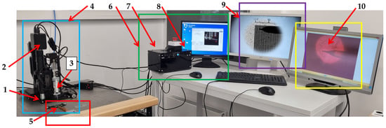
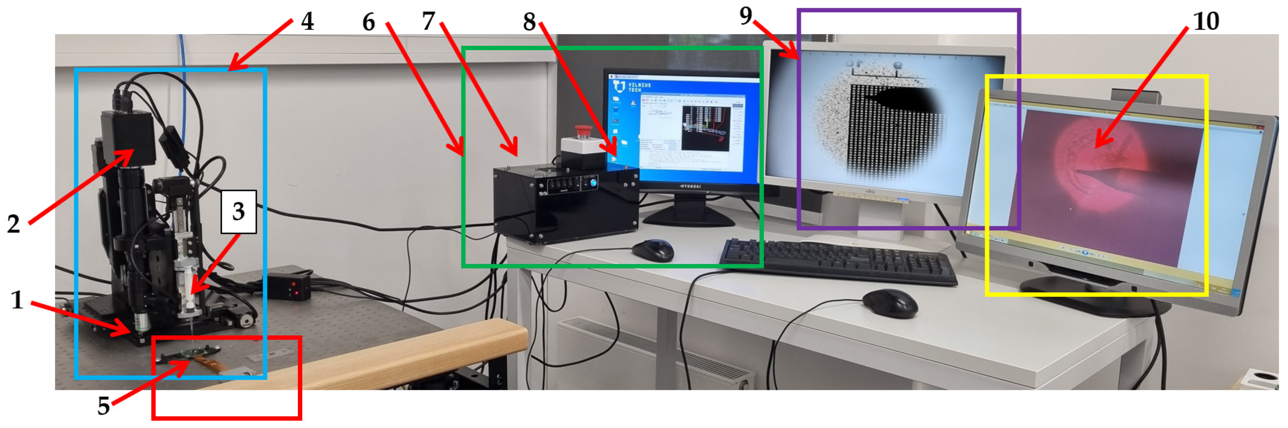
The main PC was used as a host controller to generate motion, perform image recognition, and scan results. The electromechanical system is based on the kinematic scheme of a typical orthogonal manipulator, such as a 3D printing or similar CNC machine. The precision of the drive is achieved by stepper motors operating in 1/16 micro-stroke mode, and the motion controller MachineKit v. 0.1 software (Free Software Foundation, Inc., Boston, MA, USA) version is adapted to LinuxCNC. An Orange Pi microcomputer was used in further experiments to determine other parameters [54]. The workplace is represented in Figure 1, except for the master/slave computers placed under monitors. The X, Y, and Z axis control motors are not marked separately, but the location of the computer software control window is visible in Figure 1, item 8 (green square). Figure 1 represents a real workplace, where all the hardware is.

Figure 1. Micro-manipulation/micro-robotic system setup. Label 1—ocular; 2—XCAM4K8MPA camera; 3—micro-positioning holder with instrument; 4—micro-positioning system on anti-vibration workstation (blue square); 5—BVS (red square); 6—microrobot manipulation station with LabView (green square); 7—Linux CNC based motion controller; 8—monitor of micro-robotic system; 9—monitor of imaging BVS signal (purple square); 10—view from optic camera (yellow square).

For SF testing, an image formed on a transparent film, PET 0.1 mm (Herma, Suzhou, China), line width 0.006 mm, measuring range 10–1000 µm, calibration grid on plastic film, calibration sample on glass, a graduated scale in 10 µm steps, or 10 µm squares of precise size were used for convenience to determine image sharpness and coordinate repetition/deviation. The glass needle with a 100 µm tip was used as an additional item to represent SF data collection, where the real view of the needle is captured by the optical microscope, and the shadow of the object is registered by BVS. Since the BVS is mounted stationary on an anti-vibration table, a plastic 0.4 mm fiber optic cable with a polymethyl methacrylate core and surrounded by fluoropolymer was used to record the deviation from the given trajectory. As a light source, we used Blue LED SMD 0603, with a peak wavelength of 460 nm (Lumixtar Electronic Technology, Shangpai Industrial Area, Baoan, Shenzhen, China), as the blue LEDs are most useful in this asymmetric synthesis system, as silicon has high quantum efficiency in the blue region and can adjust XCAM imager interpretation based on environmental scattering conditions. The blue light represents clear signals even without optics and enables IMX477 to detect reflections, shadows, scattering in the environment, flicker, or light intensity. This choice turns the system of these two CMOS sensors, when one of them is in the optical camera, into a global illumination sensor that complements the detailed image of the XCAM. In principle, such a fusion IMX477 with XCAM can be used to control the exposure, white balance, or processing modes of the XCAM. This is especially relevant when recording biological semi-transparent objects, such as single-celled organisms in their aquatic environment.

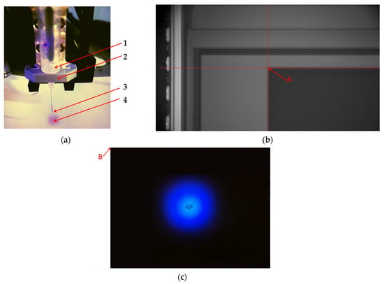
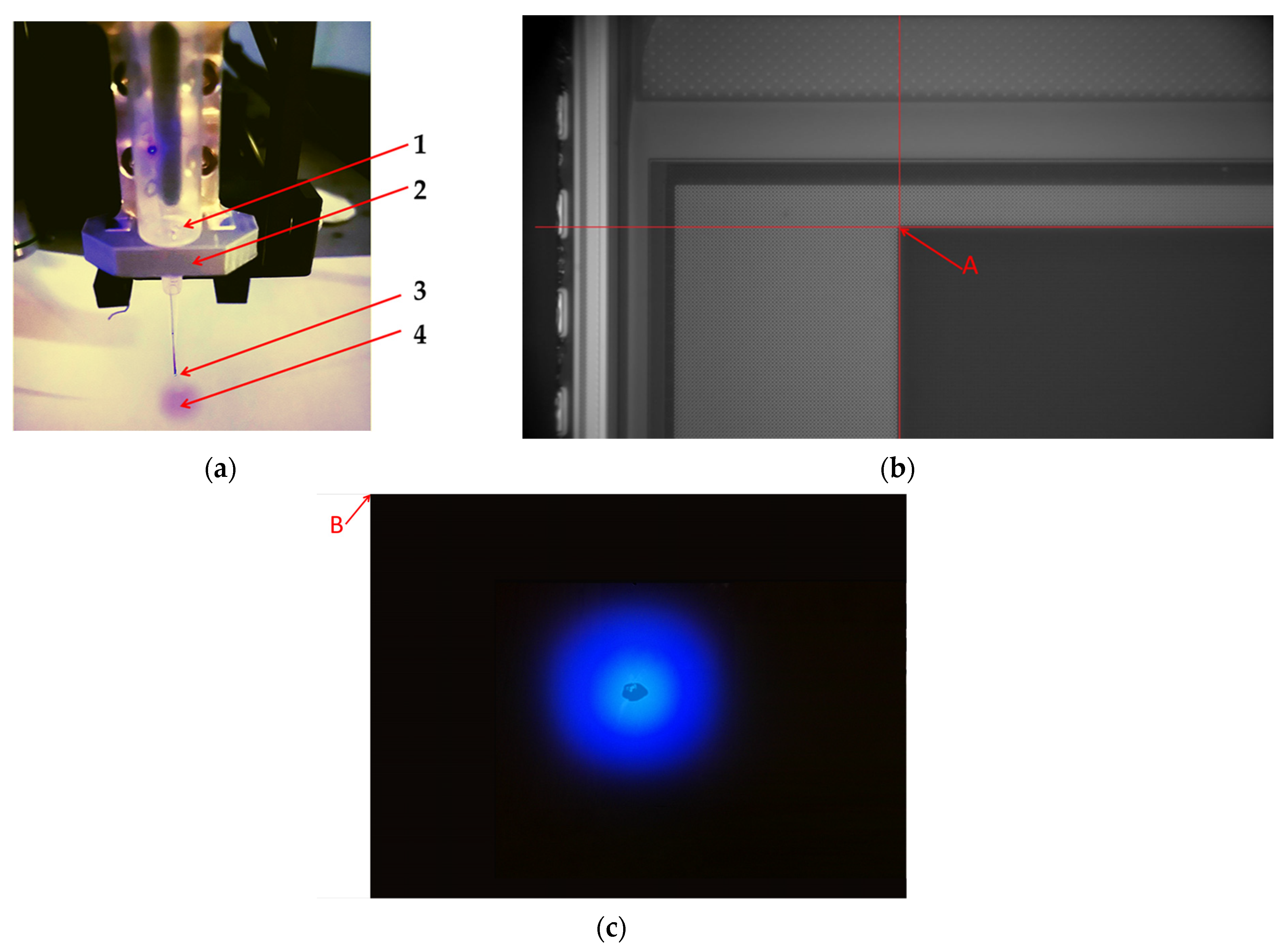
The experimental setup consists of: BVS mounted (Figure 1) on an anti-vibration table, a transparent micrometric calibration plate with a known pixel-sized dot marked on it, an optical robotic system with a slot for mounting an optical camera, and an instrument-mounting slot at a fixed distance, in which a fiber optic cable as a light source from an LED lamp is installed, with adjustable lighting intensity. Figure 2a represents an enlarged view of the workplace similar to Figure 1 point 3, where the instrument is installed (Figure 1 point 5 vs. Figure 2a) in a holder of a micro-robotic system, and the sample caption in LED light is represented in Figure 2c. The needle is replaced by a built-in fiber optic cable that transmits light of a known wavelength from a blue LED. This setup is needed to imitate and check the instrument position.

Figure 2. The representation of the workplace. (a) Label 1—the instrument; 2—the instrument mounting holder; 3—optic-fiber mounted in plastic holder; 4—the illuminated surface area from the LED light is transmitted through a fiber optics; (b) red arrow mark default position captured by optical microscope and the 1st pixel; (c) red arrow mark pointing to 1st pixel of BVS is default position of XY motorized stage.

All samples to perform the investigation were mounted on the microscope stage permanently for all time of experiment and the initial “zero” point. Initial position “0” was set using X, Y coordinates of the motors of the micro-robotic system in the LinuxCNC control system. For intermediate assessments of image quality, IrfanView 64 Image Viewer (64-bit version, Irfan Skiljan, Vienna, Austria) and similar software were applied.

2.2. Methodology and Calculations of the Investigation

Unlike encoders, video cameras are detectors of direct observation of the target and the movement path. While encoders measure only the movement of linear stepper motors. The vision systems can directly observe the actual position of a target or feature relative to the optical path, so if any type of mechanical error occurs, then something detectors like vision system cameras themselves can detect. The comprehensive error model for micro-manipulation systems must be established to consider all of the distortion that exists in microscopic nonlinear imaging.

Methodology is used to calculate the displacement of the drive. Images were taken before and after the drive returns to the start, and then they were evaluated in a MATLAB R2025b (MathWorks, Natick, MA, USA), code there we convert the image to gray style image (black and white) to a bitwise array stating 1 for white and 0 for black, allowing us to detect the position of the shadow of the needle probe then a center point of this array was found for each image.

Radius r defined:

$$r=\sqrt{{dx}^2+{dy}^2}$$

(1)

This defines a circle with radius r. Our drive will end up on this circle based on the value of r. The mean value (Formula (2)) of r is calculated:

$$r_m={\displaystyle \frac{{\displaystyle {\sum }_{i=1}^n}{r}_i}{n}}$$

(2)

where r_m is the average return, r_i is the individual return, and n is the total number to be averaged.

The absolute error is calculated using the value (r_m) of the results as the expected value, then the absolute value is calculated from Formula (2):

$$A_m=\left|r_m-r\right|$$

(3)

where A_m is the absolute error between the measured value and the true value.

The standard deviation of the result is calculated using:

$$\sigma ={\displaystyle \frac{\sqrt{{\displaystyle {\sum }_{i=1}^n}{(r_i-r_m)}^2}}{n-1}}$$

(4)

Formula (3) and value $\sigma$ represent the sample standard deviation of individual points and how far each point is from the average. It is used to calculate the average amount of variability in a data sample, indicating how much the data points are scattered from their mean. The experimental standard mean deviation S_md is calculated by the following formula:

$$S_{MD}={\displaystyle \frac{r_1-r_2}{{SD}_{pooled}}}$$

(5)

where SD is standard deviation and x₁, x₂ are experiment points.

Using the final value of measurements is shown as the sum of the mean of measured values plus the random error expressed:

$$r_m\pm \Delta m_{v,n,p}$$

(6)

represents a measured or calculated value, the coordinate and pixels in our case, with its associated uncertainty or measured value ± deviation.

On the left side of BVS (while the camera is in the left position, corresponding to the instrument), near the BVS left top edge (about 50 mm by X and Y axis), the same calibration microgrid (4 µm between lines) was placed.

The top camera (Figure 3a, pos. 1) captures an object’s photo through the optical lens. This camera was calibrated: 20 photos with precise calibration microgrid, including black parallel and perpendicular lines, where the distances in both directions between grid lines were 4 µm represented in the text below.

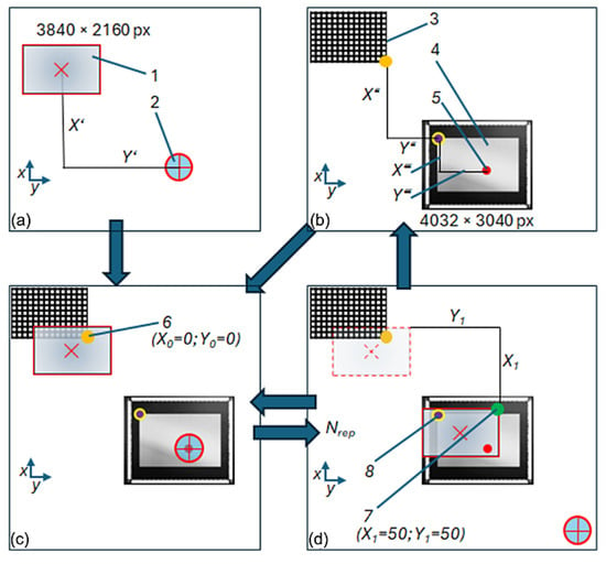
Figure 3. Measurement schemes: (a) Top frame (instrument and image from top image sensor); (b) bottom frame (calibration grid 4 µm and BVS); (c) initial measurement position with data fusion from top and BVS; (d) end measurement position in Nrep repetitions. Label 1—top image sensor; 2—instrument; 3—calibration grid; 4—BVS; 5—target point; 6—initial measurement point, in orange color (X₀ = 0; Y₀ = 0); 7—end measurement point, in green (X₁ = 50; Y₁ = 50); 8—point on top left edge of active pixel; X’ and Y’—unknown coordinates between top image sensor centrum and instrument centrum; X″ and Y″—unknown coordinates between calibration grid right bottom edge and image sensor first pixel left top edge; X‴ and Y‴—unknown coordinates between left top edge of image sensor first pixel to target object center.

Calibration is performed using a line-based grid target composed of orthogonal black lines with known spacing (Figure 3b, position 3). A specially designed ‘Python v.3.12.13’ (Python Software Foundation, Beaverton, OR, USA) script calculated calibration parameters, like RMS error, pixel anisotropy, and distortion. Instead of traditional chequerboard corner detection, this approach relies on robust detection of perpendicular line sets using CLAHE (contrast-limited adaptive histogram equalization, OpenCV) with confidence intervals (95%) for µm/px for both the X and Y directions.

With a special Python script and calibration parameters, the last image was undistorted. After this, the position of the related object was recalculated at the end of the trajectory. The BVS was also checked for calibration with the same precise calibration microgrid, but it is stated not to be calibrated, as it does not have optics, and each pixel corresponds directly to the near distance placed pixel object.

On the next step (Figure 3d), the top camera with lens and on the same frame, the instrument together with the control device was moved until this camera could see the top left edge of BVS sensing pixels (Figure 3; item 8). On the same image could also be seen the target object (Figure 3; item 5). The point on the sensing pixel edge was set as the one point for movement on the control device (software ‘LinuxCNC’, linuxcnc.org). This point (Figure 3; item 8), with some errors, corresponds to the end point of the trajectory.

The optical scanning microscope and BVS, as a comparative system, can merge visual information, providing information about samples from both sides. It is especially useful for semi-transparent objects (Figure 3c). Investigation of samples in this way reveals system positioning accuracy by recording detailed information directly with feedback. There are two ways to achieve accurate positioning of the instrument.

First method: If the medium of the research object is not transparent, the experiment starts with scheme d (Figure 3). When finding the top image sensor to find the target object, measure the distance X‴ and Y‴, moving by distance X₁ and Y₁, and by scheme b, calculating distance X″ and Y″. The next step is to move to scheme C and repeat again to scheme D, to place the instrument precisely in the center of the object several times.

Second method: If the medium of a research object is transparent or semi-transparent, the BVS (Figure 3b) can locate the test object. With the top image sensor (Figure 3a), move the instrument to the position (Figure 3c) so that the shadow of the instrument is visible by the BVS located near the test object. With the upper image sensor (Figure 3a), move the instrument to a position (Figure 3c) so that the instrument or its shadow is visible from the lower camera located near the test object. At the same time, the upper sensor can see the calibration grid. The sensor signal blur will be used to calculate the distances. After several repetitions (Figure 3d), the instrument can be positioned exactly in the center of the target.

Totals are three unknown distances (Figure 3): between the top image sensor centrum (1) and instrument centrum (2); between calibration grid right bottom edge (6) and image sensor first pixel left top edge (item 8); and between left top edge of image sensor first pixel (8) to target object center (5).

2.3. Experimental Design

The screening was conducted to optimize parameters that affect the process accuracy, including deviation caused by accidental environment influence: temperature fluctuations, moisture, building vibrations, etc. Design of experiment (DOE) is a statistical tool elaborated to plan the experiment. The required experimental success from input to output has materials, devices, methods, measurements, qualified staff, software and requires great process understanding. Data collected systematically on influencing factors helps quantitatively describe phenomena of observation. The steps of experiment planning: hypothesis, identified variables, experiment design by determining factors, experimental design, preliminary experiments, routine experiments, data collection, and conclusion validation. To obtain DOE results, one must set objectives, select process variables, select an experimental design, implement the design, verify that the data meet the experimental assumptions, analyze and interpret the results, and use/report the results that can lead to further research or DOE. The main steps of experimental planning establish a procedure in scientific research works [55,56,57,58]. According to the established procedure and information found in scientific publications, we have presented an experimental design.

3. Results and Discussion

Screening Experimental Results

The three-dimensional micro-positioning stage was elaborated for the SF model to investigate the ability of accurate repeatable motion to selected coordinates. The micro-positioning stage consists of a platform, 3-DOF, and coordinate control motors with half-micrometer step accuracy.

Images were taken before and after the drive returned to the start, and then they were evaluated using MATLAB code. There, we convert the image to gray style image (black and white) to a bitwise array stating 1 for white and 0 for black, allowing us to detect the position of the needle probe, and then a center point of this array is found for each image. The center point has a position in X and a position in Y measured in pixels and to get the displacement in X and Y, subtract the counterpoints in X and Y directions to get the displacement.

An experimental study of a selected object requires changing the instrument to perform actual manipulations with the object, where the first step is investigation by optical microscope, the next step—engineering actions performed with micro-instrument, for example a microelectrode, and the last step—optical evaluation of the engineering result on sample, when optical microscope and micro-instrument are mounted on the stage at certain distance of each other. This sort of investigation requires precise repetition of the coordinate after each action. For this purpose, a transparent film was selected with a high-resolution pattern for optical system calibration. The data processing was performed according to previously represented protocols. To represent the distance from a point to the origin in 2D space, the classic Equation (1) was applied.

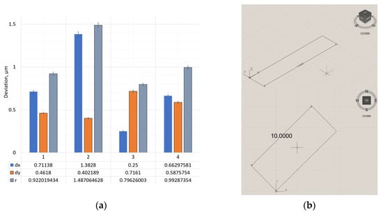
Deviations of the instrument under linear travel are graphically depicted in Figure 4a, and the shape and position of the trajectory are represented in Figure 4b.

Figure 4. Deviation of X, Y directions and radius hitting the intended coordinate—r on linear trajectory when (a) (1) speed is 50 mm/min, (2) 25 mm/min, (3) 12.5 mm/min, and (4) diagonal X/Y 50 mm/min. (b) Trajectory: Linear; F = 10.000 above, trajectory diagonal below.

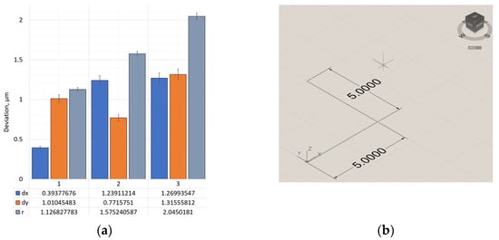
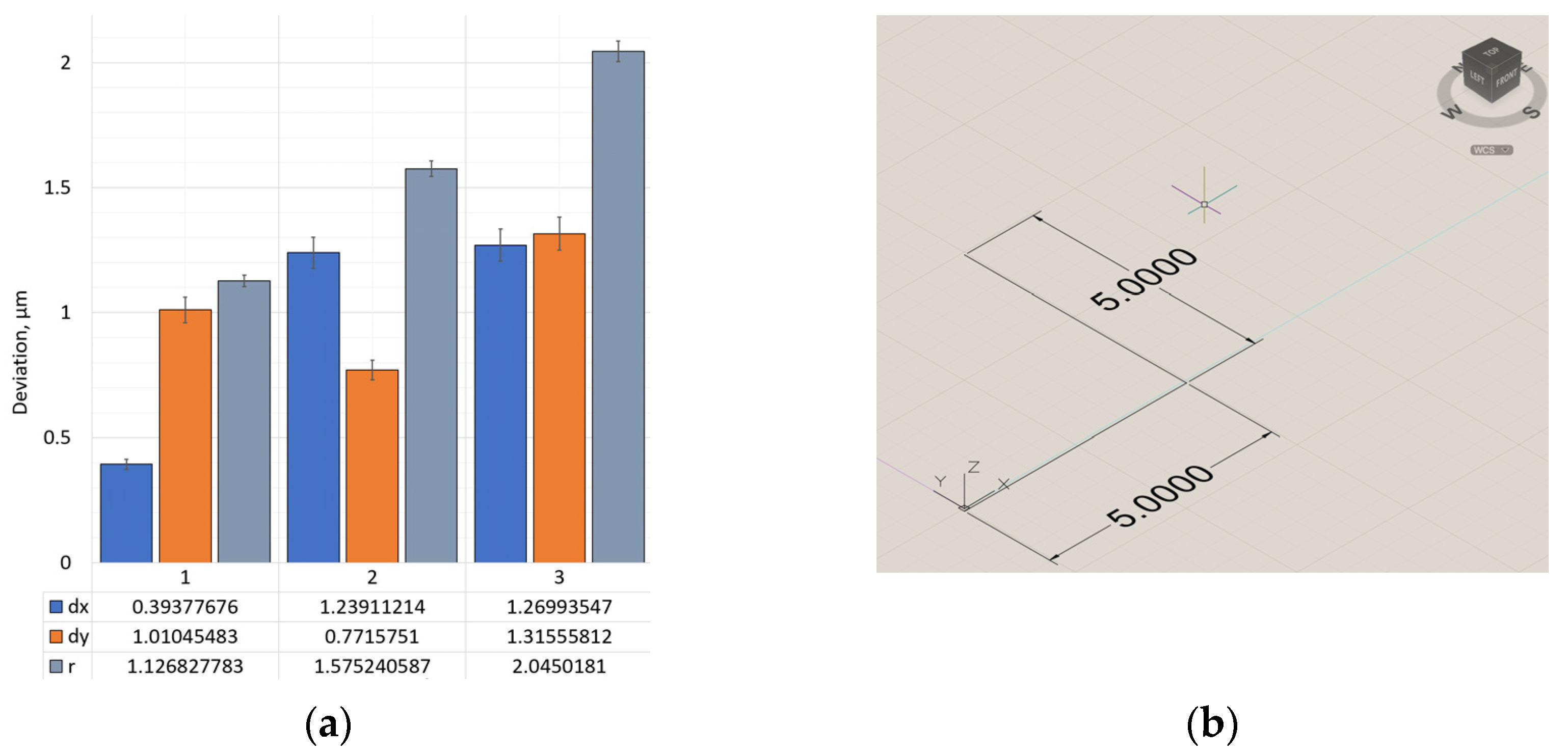
A change in the trajectory of the instrument movement gives different results. Figure 5 provides deviation along axes X and Y in Figure 5a, and the shape of the trajectory is shown in Figure 5b.

Figure 5. Deviation of X, Y directions and radius hitting the intended coordinate—r on L-shape trajectory when (a) (1) speed is 50 mm/min, (2) 25 mm/min, and (3) 12.5 mm/min; (b) L—shape trajectory.

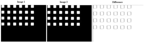
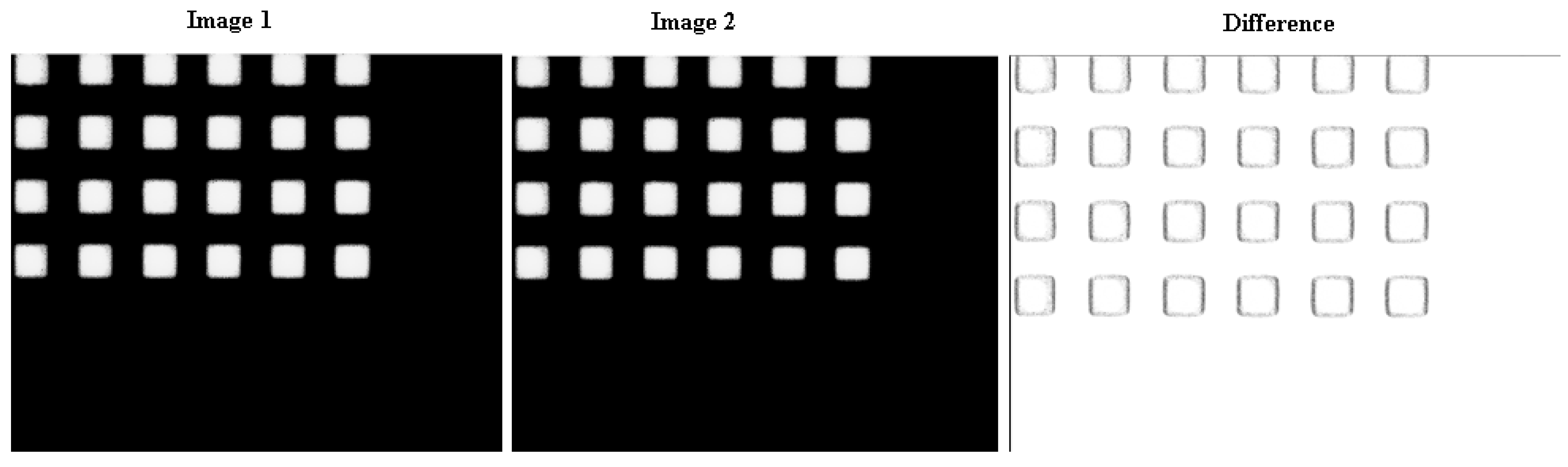
The sample data fusion of the initial image before micro-robotic system movement and the final image after movement according to the given trajectory, represented in Figure 6, where mismatched pixels are marked with a white circle. After conducting all detailed evaluations of the results obtained, it was selected to demonstrate the hypothesis and its realization using a linear trajectory and the most complex one: a spiral.

Figure 6. Calculated absolute difference in pixel from the initial view of the target, where (image 1) image before the micro-positioning stage moving, (image 2) is the picture after the trajectory is completed, where the trajectory: to walk diagonally for 200 mm in 0.5 µm increments and return to the starting point; the difference picture provides graphically non-coincident edges from positioning error of the microrobot.

After assessing the probability of deviation from the planned trajectory, we performed an assessment based on the pixel mismatch in the images obtained before performing the movement task according to the selected trajectory and returning the probe to its original position. As we can see from Figure 6, the pixel mismatch represented a black dot around it.

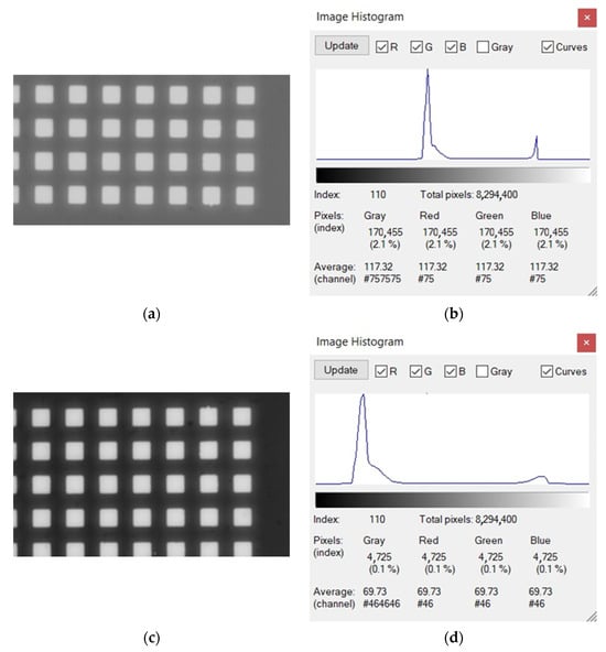
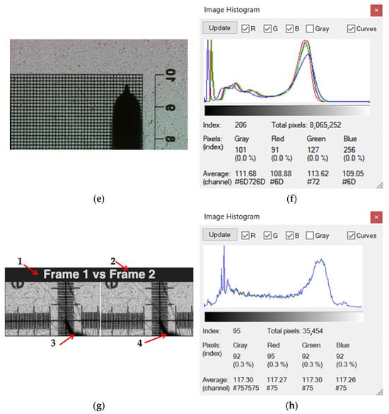
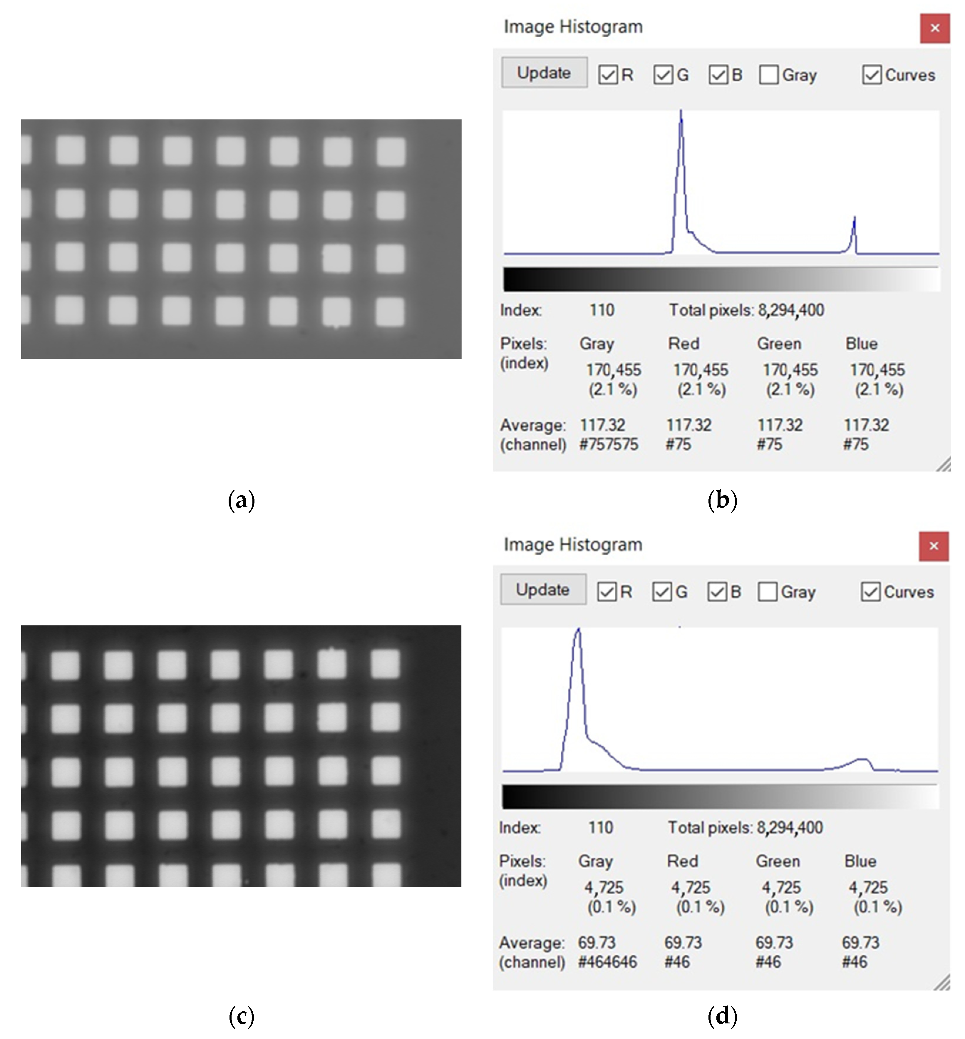
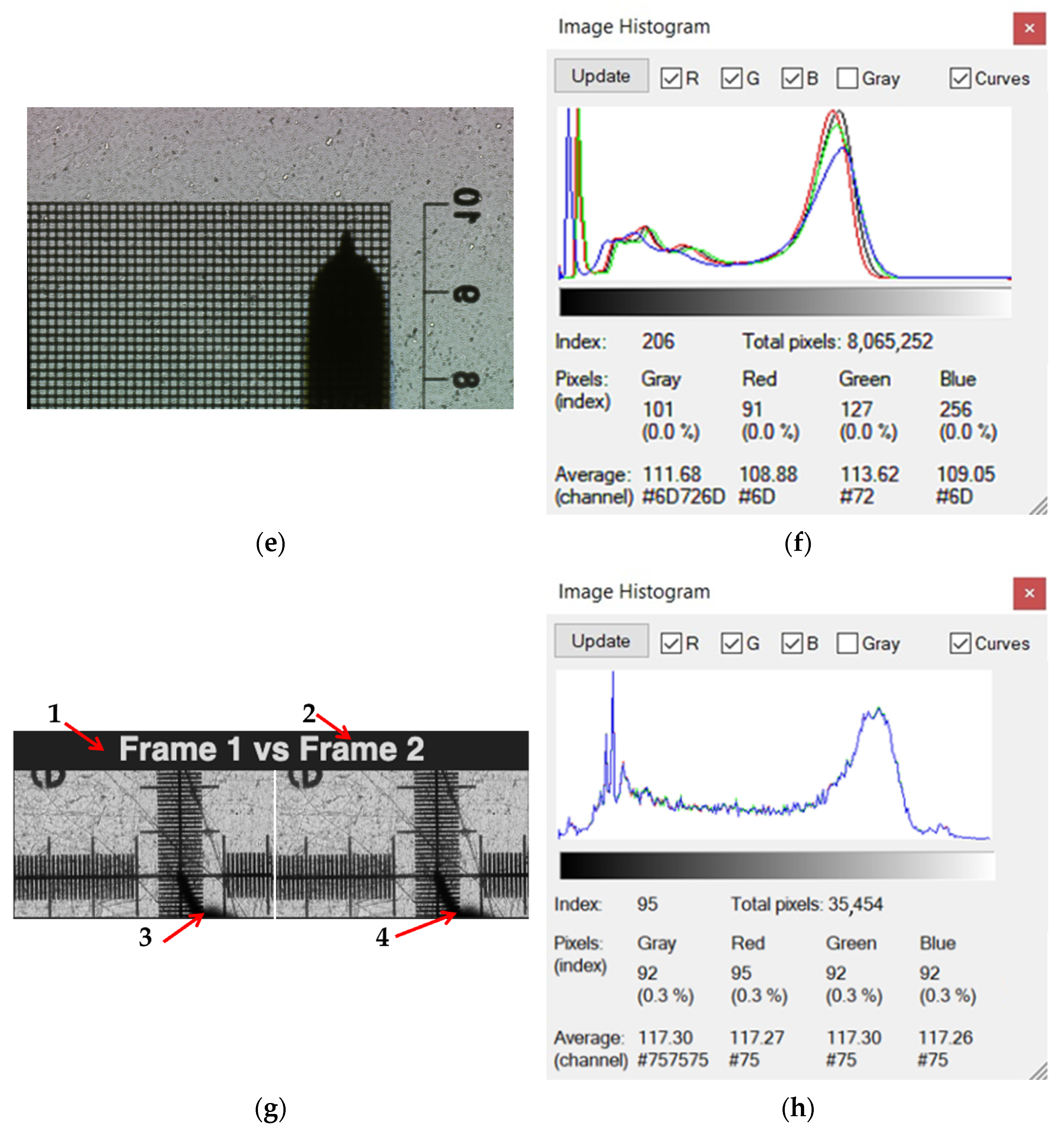
Typically, the peak on the left of the histogram represents underexposed or lost details, and the right peak represents overexposed. The peak distributions represent noise characteristics/patterns. In our experiment, the IMX477 (without optics) acts as a global light/spectral sensor, while the XCAM4K8MPA (with optics) provides a detailed image, as can be clearly seen from the histograms (Figure 7). In principle, one way to achieve information fusion can be realized using histogram information; these two streams can be combined. Using the histogram of the IMX477, adjusting the exposure of the XCAM, exposure-controlled fusion is possible. The histogram of the IMX477 image, using blue LEDs, provides a stable reference point for illumination shift, while for color-based fusion, scatter detection can be implemented based on this histogram. Since the histograms of the blue channel are extremely sensitive to defects, it is necessary to increase the contrast of the BVS image. Also, if the goal is only image data fusion without evaluating the deviation of the micro-robotic system from the given trajectory, the IMX477 histogram can be used, and XCAM processing modes can be applied. The resulting photos were obtained using an optical microscope and BVS; without optics, images were evaluated by processing the photos with several programs. The histogram was obtained with the program IrfanView64 Image viewer, for preliminary data assessments. Visual differences in the captured view recorded by the optical microscope and BVS are represented in Figure 7e. In Figure 7g, the instrument is visible on the calibration grid. Two images of IMX477 without the optics are not dealing with “images” in the usual sense, because in this case, the BVS acts as a global light/spectral sensor, so each frame is essentially a 2D measurement of illumination, not a spatial image. This completely changes the fusion strategy because a variant amount of information can be extracted from “lens-less images” and combined into a single, more meaningful signal (Figure 7g). Hence, because there is no optical lens, each frame captured by BVS is a global photometric map, influenced by overall brightness, spectral content, scattering, reflections, and sensor noise; no spatial structure is meaningful. But the statistics of the frame are extremely useful. Data fusion from two IMX477 frames is possible: global brightness fusion by calculating the average intensity of each frame. The data fusion in this case provides a reliable estimate of the illumination, smoothing out noise. Hence, it is possible to assess the reliability of the image against such an image using the deviation of the robotic system instrument from the given trajectory. Spectral fusion is relevant only if different LEDs are used and are suitable for spectral fusion, but in our case, such a solution is less reliable.

Figure 7. Evaluation of images captured by optical microscope and BVS by investigation of parameters in histograms. (a) BVS view of object; (b) BVS view histogram; (c) image from optical microscope, gray; (d) histogram of optical image; (e) BVS, view of calibration grid and a shadow of instrument on the calibration grid, when distance of instrument from surface: z = 5 μm, the instrument tip size R = 200 μm; (f) the histogram of BVS image; (g) the image, where (1) “Frame 1” before movement of instrument; (2) “Frame 2” after movement of instrument; (3) the shadow of instrument captured on calibration grid before movement; and (4) shadow after movement of instrument; (h) the histogram of photography.

In Figure 7, the images were collected to illustrate the main research methods and techniques, collected by an optical camera and BVS with the calibration grid placed directly on the BVS (Figure 7a). At the point of intersection of the coordinates, we observe the shadow of the needle inserted into the slot of the manipulation instrument (Figure 7e,g). The color shift observed in Figure 7g image when a transparent film was observed is because the thin film acts as a thin-film interference filter. A higher resolution image of the raw calculation program is presented in Figure 7g. Since the calibration curve, like the BVS, remains in the same position during instrument movement, the change in the location of the instrument shadow is directly related to the errors that occur when the micro-robotic system performs actions and moves along the assigned trajectory. After conducting a study where an ultramicroelectrode was mounted in the holder of the micro-robotic system, and white light illumination was used for the entire workplace, another lighting method was chosen, where the entire environment was unlit, and a fiber optic cable mounted in the holder instead of the electrode was used as the main lighting.

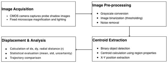
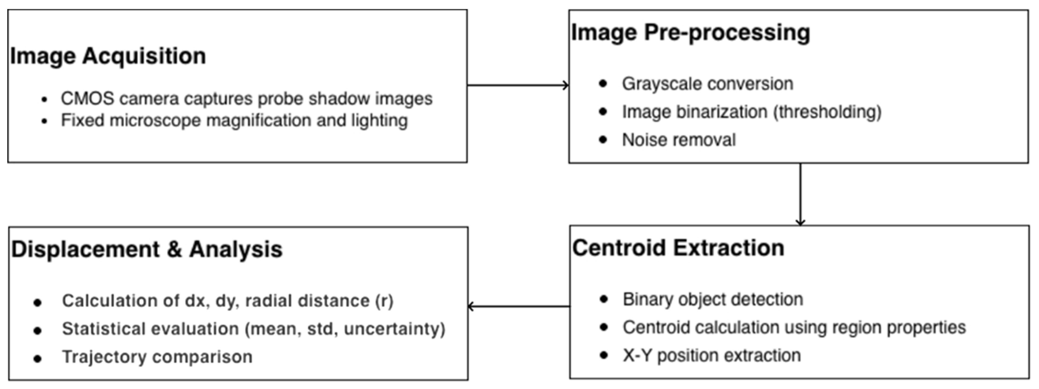
Figure 8 shows an image processing algorithm in MATLAB. This algorithm performs image pre-processing through thresholding and noise removal to isolate the target, then executes centroid extraction to determine precise X-Y coordinates for each frame. Finally, the script performs a displacement analysis to calculate radial movement in microns and evaluates the data using statistical metrics.

Figure 8. Workflow of image processing algorithm in MATLAB.

One of the difficulties is the fusion of data with different pixel counts when evaluating the same image obtained with an optical microscope and the BVS. We have decided on a detail of the gradation scale, where we see 100 µm-sized squares. We also see plastic defects that occurred during manufacturing. When the images were obtained with an optical microscope, the pixel size was smaller than the pixel size of the BVS. In this case, the discrepancy in the resolution of the image results is due to pixel dimension errors.

This graph shows the center-of-intensity positions computed from the acquired snapshots, representing the motion of the end effector (needle tip). The displacement after each consecutive snapshot is obtained by subtracting successive position values along the Y-axis. The red curve indicates a polynomial fit to the measured displacement, highlighting the overall motion trend.

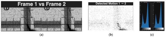
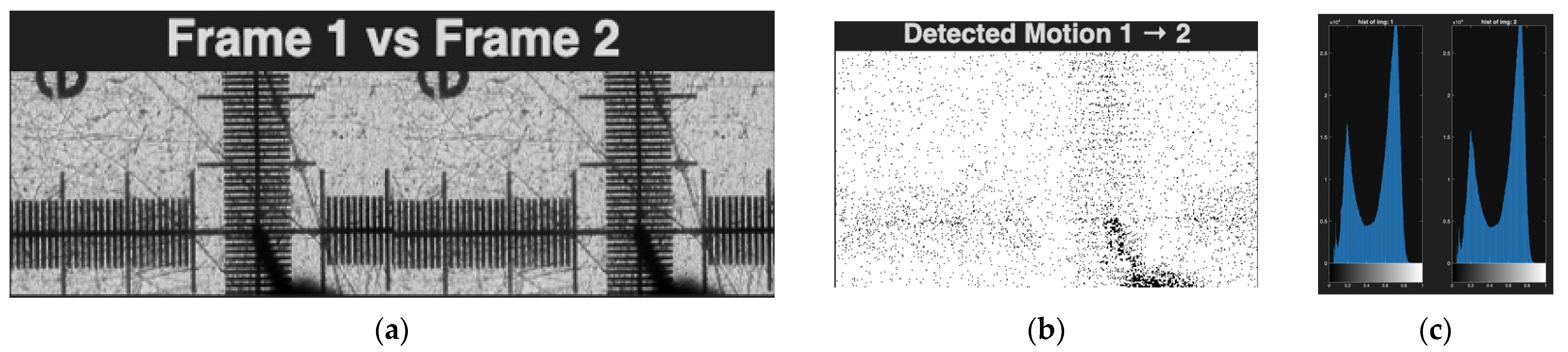
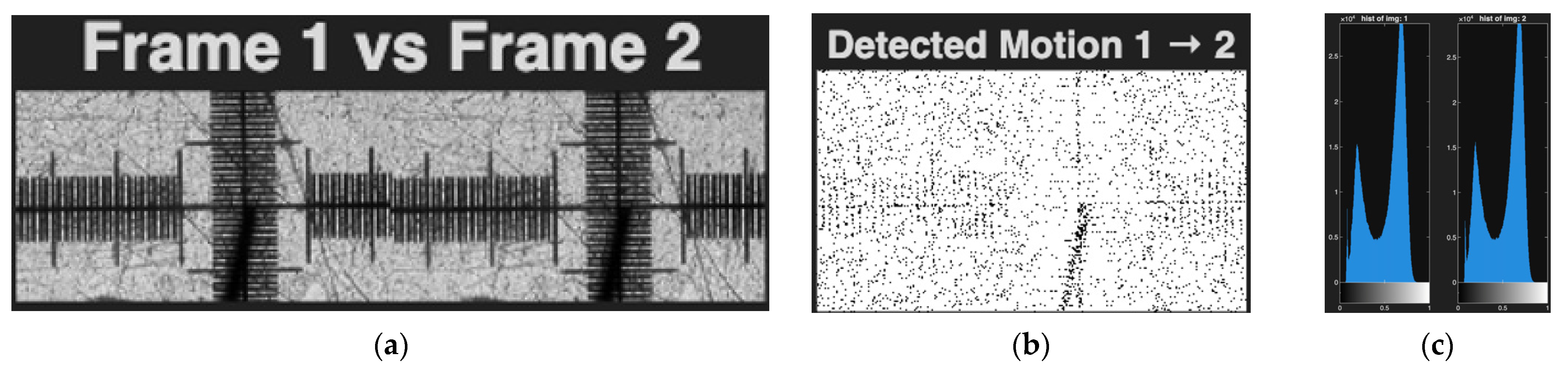
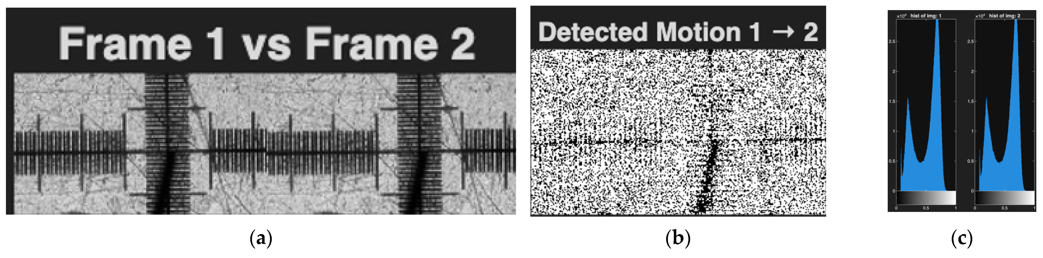
Figure 9 illustrates three different analysis windows. From left to right, the first panel (Figure 9a), titled “Frame 1 vs. Frame 2”, shows snapshots acquired after the 1st and 2nd of completed motions, respectively. The second panel (Figure 9b) displays the pixel-wise difference between these two frames, highlighting the displacement of the needle between consecutive motions. The third panel (Figure 9c) presents the intensity of histograms corresponding to the snapshots taken after the 1st and 2nd motions. This example demonstrates the analysis performed on two consecutive snapshots. Similar image pairs are acquired and analyzed after each motion to quantify the drive precision. The L-type trajectory (Figure 5), speed 50 mm/min, was investigated 30 times, with the whole calculation represented in the text above. Experiments were performed at movement speeds of 50 mm/min, 25 mm/min, and 12.5 mm/min, L-type trajectory, and no significant differences were observed in the detected motion. Therefore, only one example of this study is presented in the text, in Figure 10.

Figure 9. The data fusion of BVS images. (a) Frame 1 before movement of instrument vs. Frame 2 after movement of instrument, (b) pixel mismatch map marked pixels with white dots, (c) image histograms, linear trajectory, speed 25 mm/min.

Figure 10. Sample data fusion of optical camera images. (a) Frame 1 before movement of instrument vs. Frame 2 after movement of instrument, (b) pixel mismatch map marked pixels, (c) image histograms, selected L-type trajectory, speed 50 mm/min.

The selected trajectory of two-axis movement, when the instrument is moved diagonally, at a speed of 50 mm/min represented in Figure 11. As we can see from the represented data, the motion detection and histograms of photography, the quality looks similar, so the pixel mismatch can only be attributed to the deviation of the robotic system from the selected trajectory. A similar pixel mismatch is observed both when moving in a straight line along one axis and when moving along two axes, X and Y, or the so-called diagonal trajectory. In this case, if we compare the first experiment and the 30th experiment when the instrument trajectory is C-shaped, we get an accumulating pixel discrepancy. This problem of robotic systems deviating from the semicircular trajectory is well known. Algorithms are often used to compensate for this problem, but increased error detection and elimination can be achieved by using data fusion even with conventional vision sensors. The experimental workplace for image data fusion is represented in Figure 12.

Figure 11. The data fusion of optical camera images. (a) Frame 1 before movement of instrument vs. Frame 2 after movement of instrument, (b) pixel mismatch map marked pixels, (c) image histograms, diagonal trajectory, speed 50 mm/min.

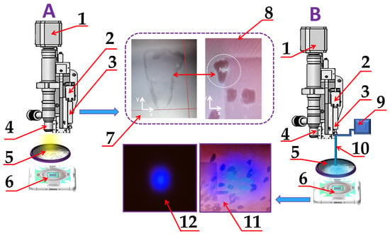
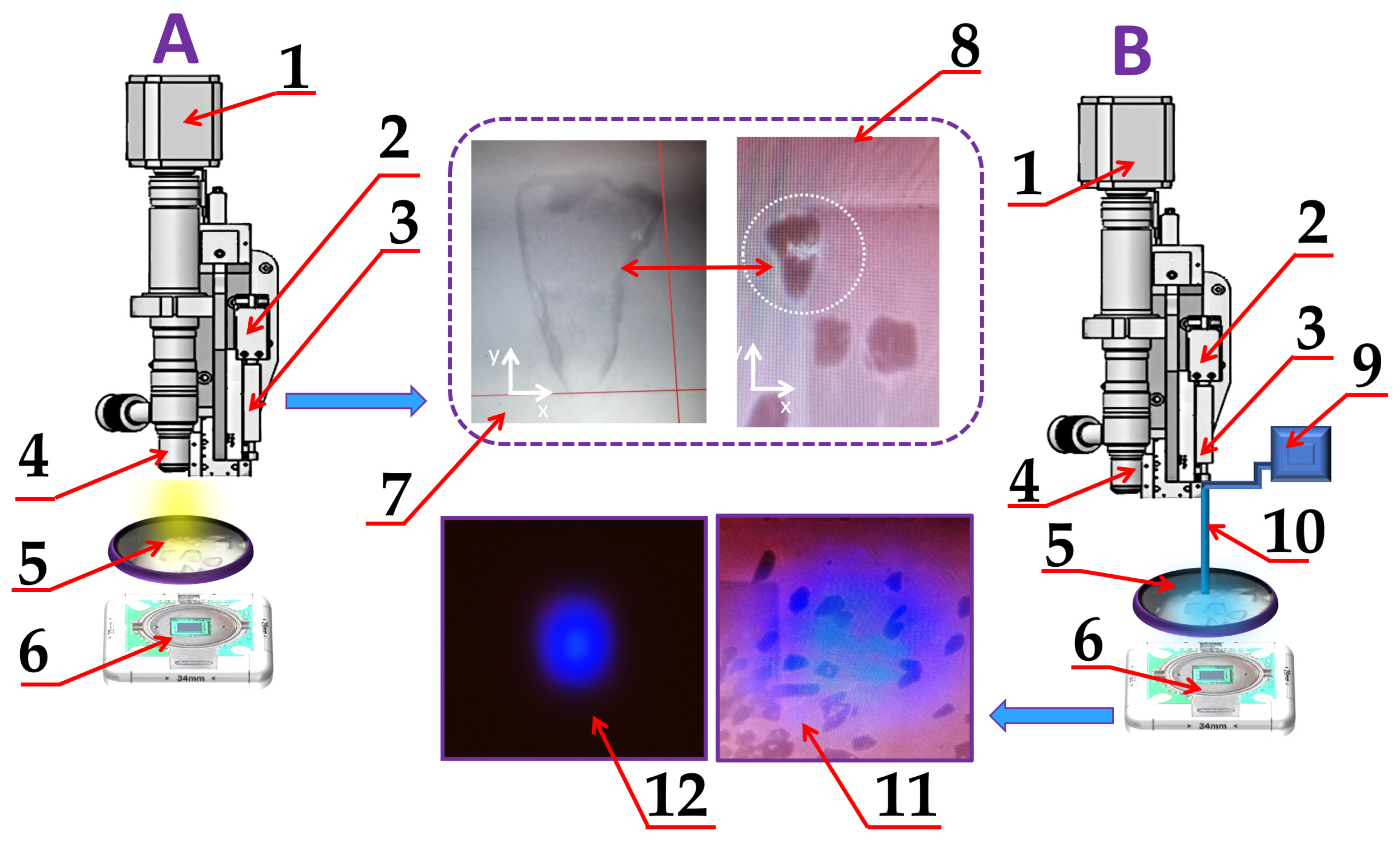
Figure 12. Visual representation of the workplace for image data fusion. (A) image capturing by digital camera with optical microscope: 1—digital camera; 2—the instrument holder; 3—the instrument; 4—optic lenses; 5—sample, 6—BVS, 7—image of sample captured by optical microscope with digital camera, 8—image captured by BVS with selected sample; (B) processing of image from BVS, where 9—blue LED; 10—fiber optics; 11—captured BVS view of samples of calibration grid using additional side light source; 12—BVS view using LED blue light.

By using MATLAB, the centroid detection was performed, also the statistical evaluation of motion precision and qualified drive displacement.

To find the centroid of light spot generated by LED with fiber optic to pixel-size accuracy, we selected Formulas (7) and (8). The I (X, Y)—the brightness of a center light spot with coordinates X, Y. The coordinates of the center of the light spot (Xs, Ys) are calculated as follows:

$$Xs={\displaystyle \frac{\sum (x\cdot I\left(x,y\right))}{\sum I\left(x,y\right))}}$$

(7)

$$Ys={\displaystyle \frac{\sum (y\cdot I\left(x,y\right))}{\sum I\left(x,y\right))}}$$

(8)

Figure 12 represents the optical image view obtained from an optical microscope with a digital camera and BVS of sieved glass pieces ranging in size from 127 μm to 177 μm. The image is displayed using side illumination with white light. The glass pieces were chosen to investigate the possibility of image data fusion when observing biological objects, such as single cells. The side-illumination in the BVS image was applied to represent all objects in scenes of observation. Selected images were used for image data fusion.

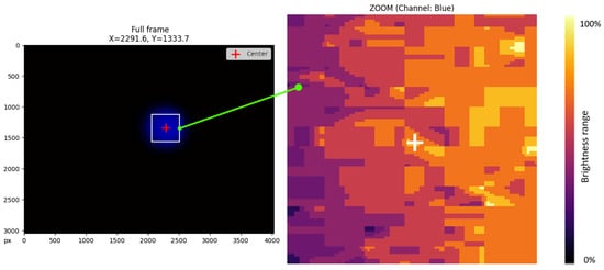
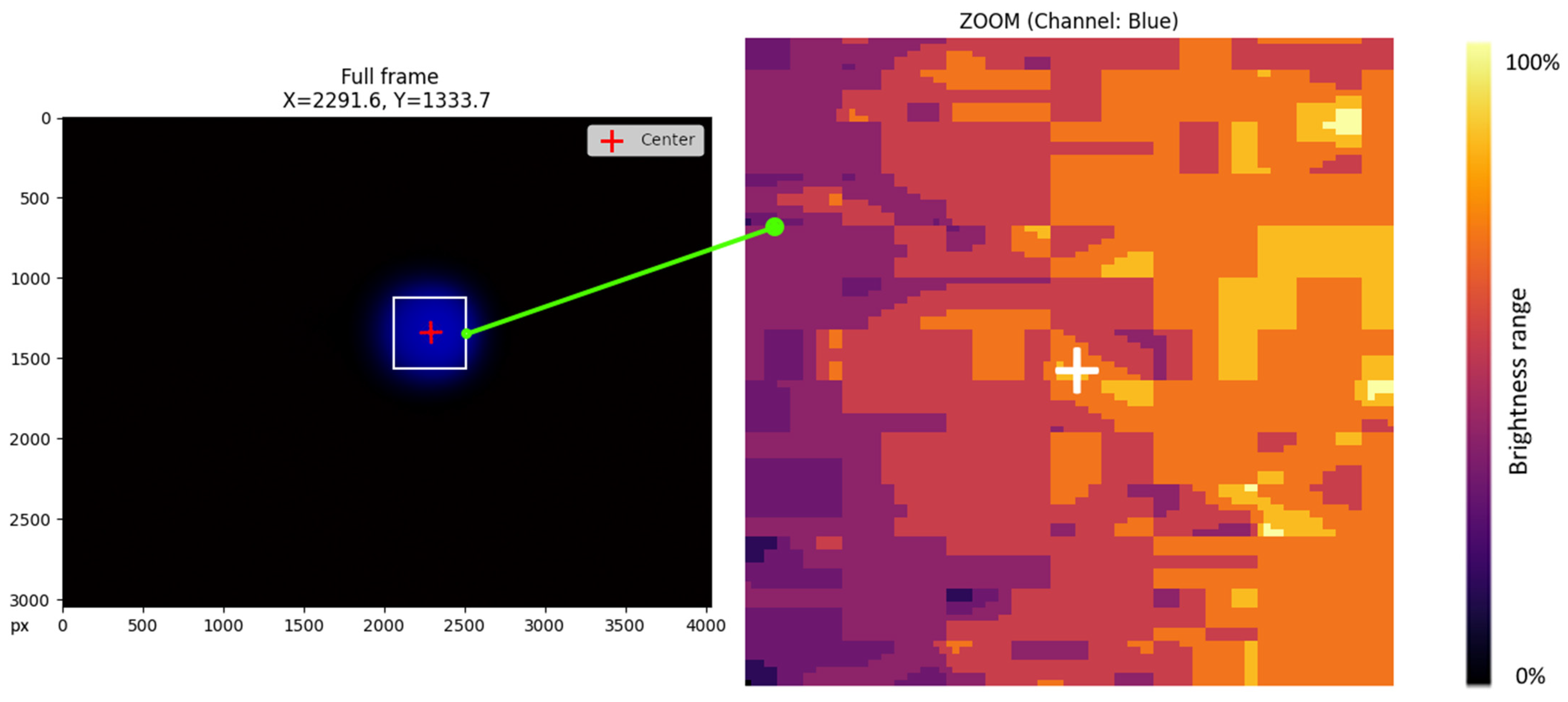
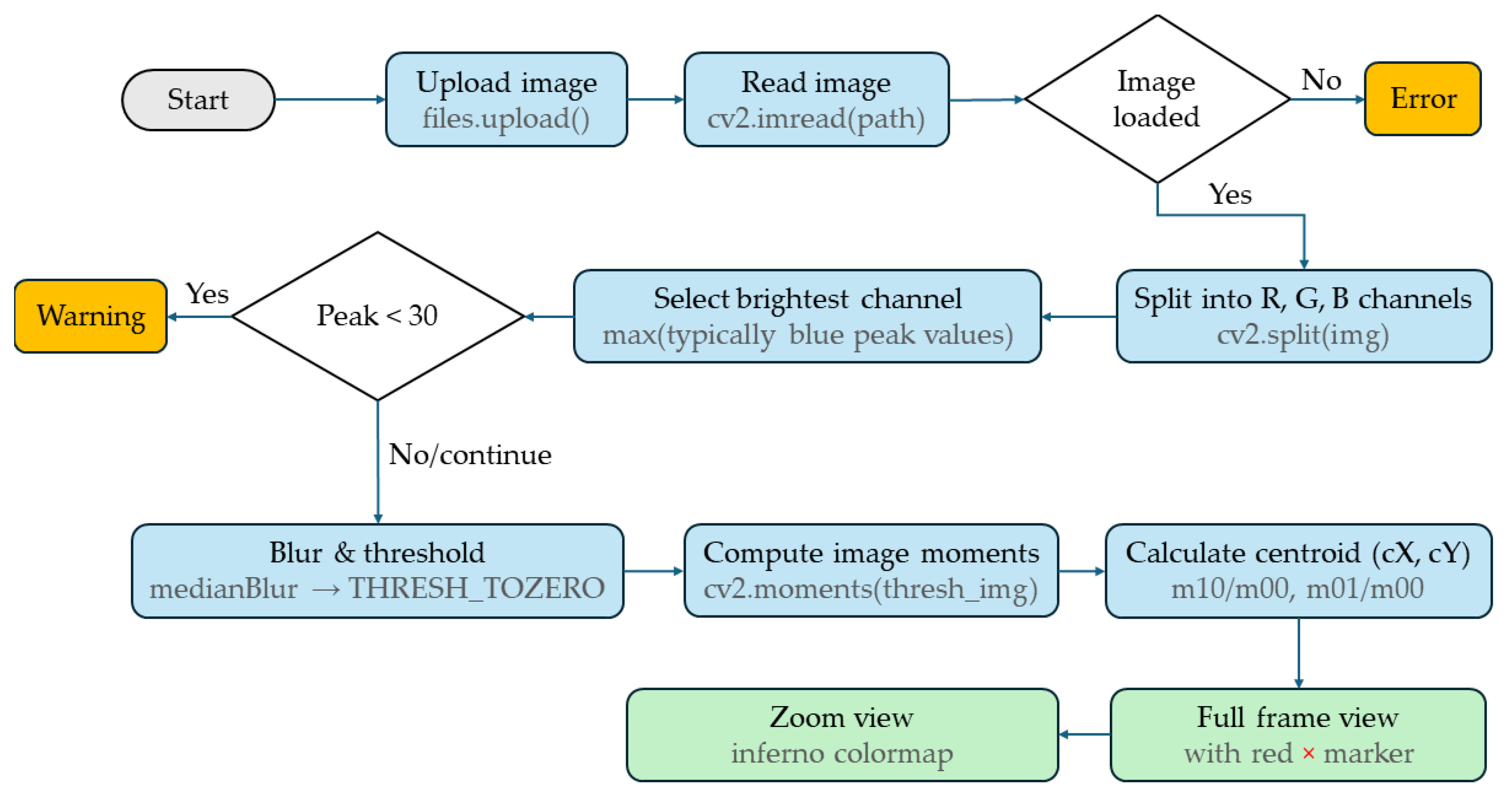
Figure 13 represents a view of the LED light on BVS and the geometric center of the instrument (in this case, the fiber optic) marked with a red cross, and the center of the light spot of the instrument brightness level range map. The summation of image data in the next step was performed over a region of interest (ROI) around the brightest spot, and the positioning result is represented in Figure 13. The algorithm of image processing in Figure 14 evaluates the positioning precision and repeatability of an XY motorized stage using a sequence of images. The algorithm calculates the cross-power spectrum of the images and applies an Inverse Fast Fourier Transform (IFFT). The summation of image data in the next step was performed over a region of interest (ROI) around the brightest spot, and the positioning result is represented in Figure 13. Sensors have different sensitivities to different wavelengths. Since the light source (LED lamp) can be monochromatic (e.g., blue), the useful signal is contained predominantly in one channel. After selecting the color channel, we perform preprocessing using a median filter. The median filter effectively removes impulse noise (hot pixels) while preserving the spectral characteristics of the main light spot. To eliminate the influence of sensor thermal noise and background illumination, a region of interest (ROI) is clipped where the intensity exceeds 50% of the maximum (Full Width at Half Maximum).

Figure 13. Visual representation of a light spot generated on the surface by an LED and fiber optic (left), the calculated and marked center of this light spot (right), realized by Python.

Figure 14. Workflow diagram of an image-processing pipeline in Python for calculating and marking the center of a light spot.

This ensures that only light from the source is included in the calculation. The center coordinates are calculated as the center of mass of the intensity distribution. This enables sub-pixel accuracy, which is higher than a discrete pixel grid. Image data fusion was performed according to the protocols of O. Vismanis [14]. The aim of the next experiment was to determine the possibilities of quantifying the actuator’s displacement. The visual results complement the analysis, including frame comparisons, pixel difference images, intensity histograms, motion plots, and polynomial fits that represent the behavior of the motor drive based on the shape of the trajectory. This method can only partially help control the deviations of the instrument from the specified trajectory; therefore, another method was chosen, more suitable for the selected task, the results of which are presented below in the text.

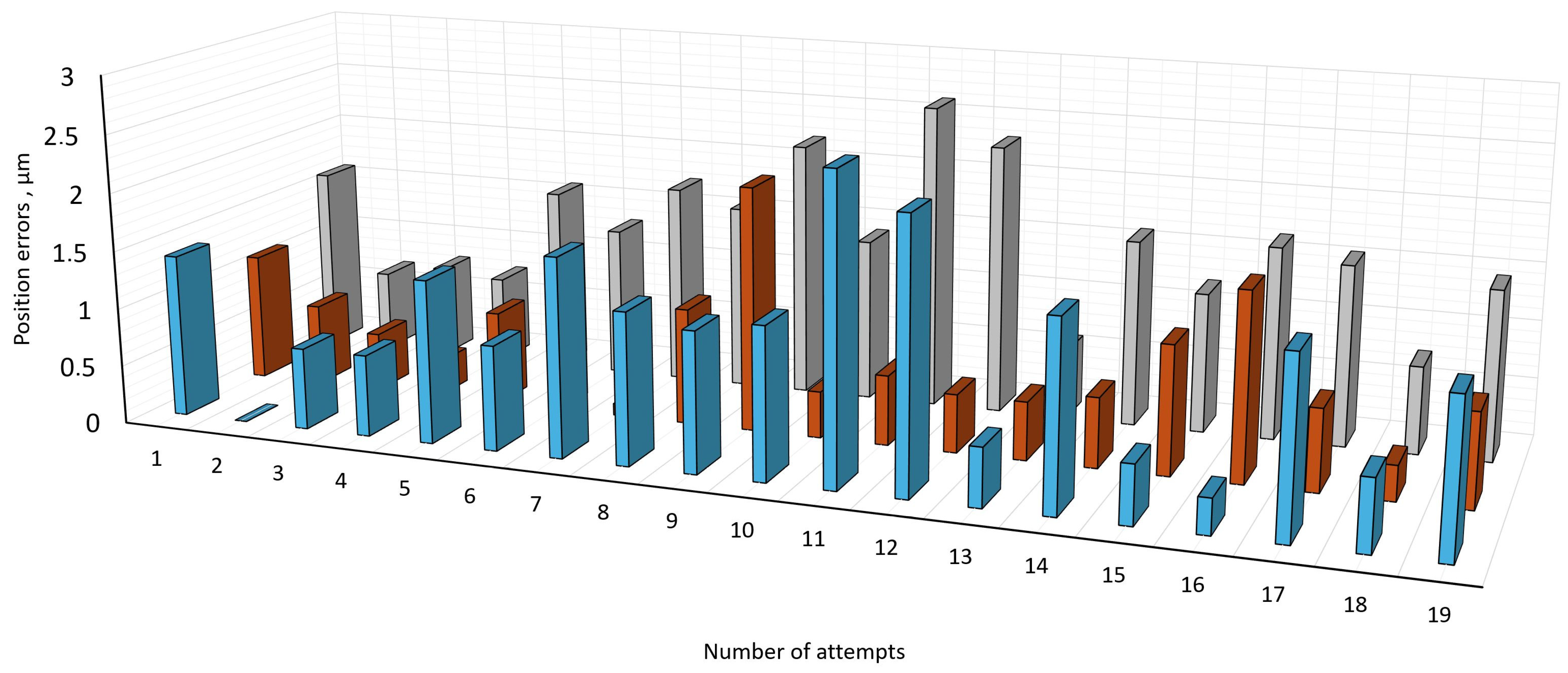
Figure 15 represents the results of errors resulting from the X-axis and Y-axis, calculated using the fusion of data from both sensors. Errors after 14 repetitions decreased because the system switched to a more stable operating mode with less accuracy deviation.

Figure 15. Positioning error distribution over repeating of movement of microrobot in the same trajectory at a distance of 50 mm by X and Y axes with a speed of 50 mm/min. Blue columns denote positioning error along the X axis; orange columns denote positioning error along the Y axis; gray columns denote total positioning errors.

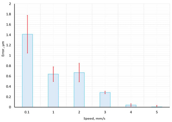
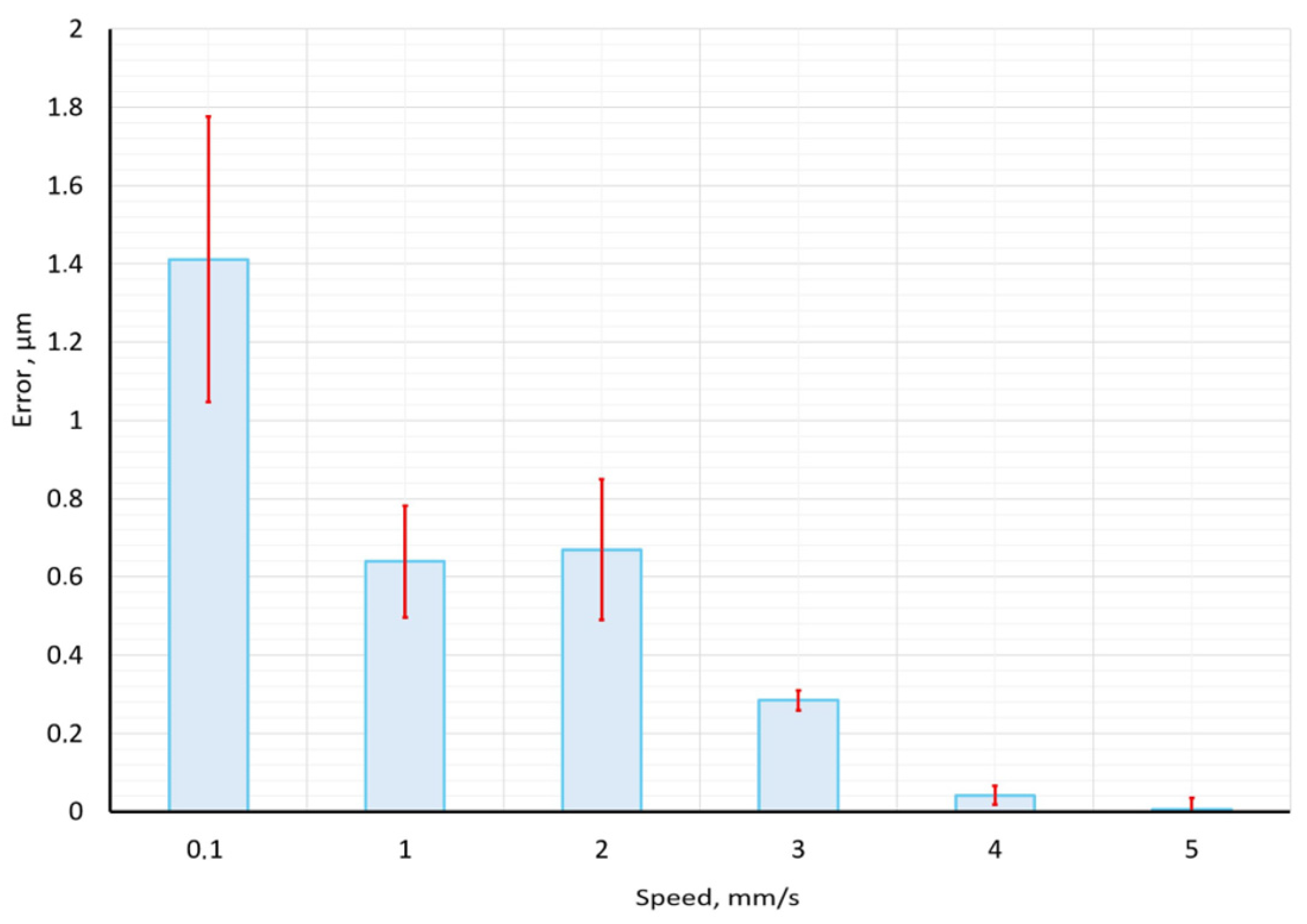
Figure 16 shows the results of experiments with different speeds of movement, from 0.1 to 5 mm per second. Every experiment at each speed was carried out 20 times. On this graph, we can see those better results and good repeatability with a speed of more than 4 mm per second. With a low speed of 0.1 to 2 mm per second, the accuracy of the X axis exceeds 1 micrometer. Accuracy in higher speed tests indicates better accuracy results, for example, microscope displacement speed 4 and 5 mm/s delivered average error below 0.04 micrometers.

Figure 16. Obtained positioning accuracy in micrometers at different movement speeds on the X axis.

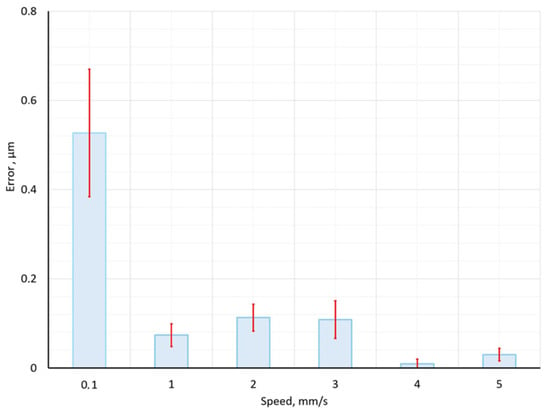
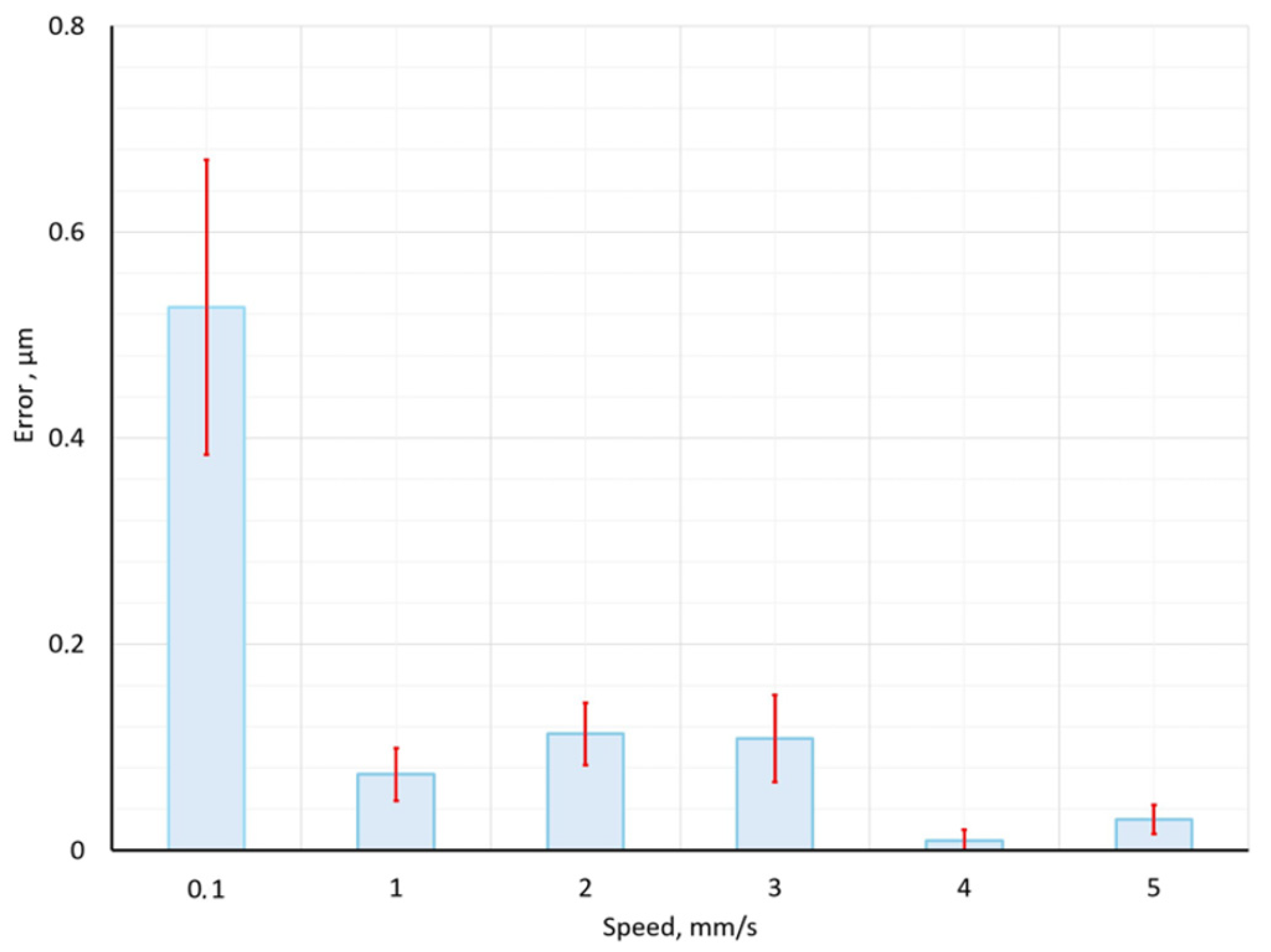
Figure 17 shows the results of experiments on the Y axis. Accuracy on the Y axis is two times more accurate than on the X axis, with all speeds from 0.1 to 5 mm/s. This accuracy can be generated by step motors and a control system; the mechanical system of the microrobot has compensated gaps and screw drives calibrated, and their accuracy and velocity are independent.

Figure 17. Obtained positioning accuracy in micrometers at different movement speeds on the Y axis.

The methodological performance of the proposed sensor fusion system was quantitatively evaluated to determine its operational robustness. Regarding accuracy, the integration of the BVS achieved a Root Mean Square Error (RMSE) of 0.25 µm, representing a 62% (from 1.3 µm to 0.5 µm) improvement in precision. However, the applicability of this method is limited by certain environmental conditions: it has been observed that the positioning accuracy deteriorates when the brightness drops too low, since the centroid extraction algorithm requires a minimum contrast ratio to maintain sub-pixel accuracy. Matlab and Python scripts process images in a few seconds and provide ready-made results for processing centroid coordinates, which then allows for calculating the difference in microns.

4. Conclusions

This investigation was based on visual data collected by a micro-robotic/micro-manipulation system identical in function to a scanning microscope, developed for live cell electrochemical engineering, containing a host computer, a three-degree-of-freedom with orthogonal manipulator, precision drive equipped by micrometer-sized pitch ball screw drives, optical system, motion controller, and main control unit. This micro-robotic system can be equipped with holders for different instruments, available for transparent surfaces and purposes of surface engineering. This paper presents an analysis of the image obtained by different methods through pixel shift based on the visual image fusion characteristics of different types of cameras for the purpose of micro-positioning quality.

Since there are many technological areas where accurate return to a given coordinate is very important for fundamental research, when observing objects smaller than one micrometer with an optical microscope, it is important to eliminate the deviation from the planned coordinate point along the intended trajectory.

We have demonstrated the system with a mounted optical microscope and conventional BVS combination for image registration on transparent or semi-transparent micrometer-sized objects. The results obtained with 0.5 micrometer accuracy may be useful for studying dynamic biological objects. The main limitation of our current method is the deviation of the microrobot from the given trajectory. Although good resolution can be achieved for spatial imaging, the main goal of automatically locating a single cell on a transparent Petri dish is still challenging, both due to the number of BVS pixels and the deviation from the given trajectory when it becomes composed of multiple directions of movement.

Our proposed method combines data from multiple vision sensors and global light/spectral sensors, where each frame is essentially a two-dimensional measurement of illumination, and can be used to estimate the deviation of a robotic system from a given trajectory when examining a semi-transparent object. The studies can be performed in solutions in transparent containers, such as plastic Petri dishes. Our chosen method can act as an aid in searching for unicellular organisms in a transparent container or in performing electrochemical measurements on the surface of cells.

SF data, which can find successful practical applications, is in great demand for robotization. We also evaluated the positioning inaccuracies; we evaluated the difference in positioning when, after scanning a part several times, it is not obvious how to find optimal values for these parameters, as the cost function needs to additionally account for model inaccuracies to guarantee optimal performance.

An optical camera and BVS were used to check positioning errors. In real experiments, the upper optical cameras can be used for object observation and investigation, determining the location of the objects under investigation, and cannot be used for the correct placement of the instrument when they are separate from each other. The lower image sensor can be used to verify the location of the instrument, where the boundaries or shadow of the instrument can be seen.

To automate the search, recognition, and positioning of the probe electrode over the selected object under the microscope, merging data from different optical systems is a very important step in microscopy. In the future, the authors plan to conduct studies with yeast or other unicellular organisms. Such work requires precise positioning and the ability to reproduce selected coordinates, while controlling deviations from the selected coordinate due to objective reasons when the motors deviate from the selected trajectory. Future work is planned to continue data fusion methods for automating single-cell detection in aqueous media and for surface engineering purposes.

The data fusion method used in this work can improve positioning accuracy when working with semi-transparent objects or with living cells, when it is not possible to simultaneously perform surface engineering manipulations and observe the object under study with an optical microscope. This method is versatile and does not require complex equipment or software, and can be used for research work using a scanning electrochemical microscope, micro-robotic systems for surface engineering operations that require an accuracy of at least 0.5 micrometers.

References

- Ruark, A.E.; Ruark, A.E. The Limits of Accuracy in Physical Measurements. Proc. Natl. Acad. Sci. USA 1928, 14, 322–328. [Google Scholar] [CrossRef] [Scilit]
- van Vliet, W.P.; Schellekens, P.H. Accuracy Limitations of Fast Mechanical Probing. CIRP Ann. 1996, 45, 483–487. [Google Scholar] [CrossRef] [Scilit]
- Kovac, I.; Frank, A. Methods for calibration and testing of flexible arm measuring devices. WIT Trans. Eng. Sci. 2025, 23, 500. [Google Scholar] [CrossRef]
- Yuan, Z.; Zhou, S.; Hong, C.; Xiao, Z.; Zhang, Z.; Chen, X.; Zeng, L.; Wu, J.; Wang, Y.; Li, X. Piezo-actuated smart mechatronic systems for extreme scenarios. Int. J. Extrem. Manuf. 2024, 7, 022003. [Google Scholar] [CrossRef] [Scilit]
- Youm, J.Y.; Youm, J.Y.; Yang, J.-M. Optical-resolution photoacoustic microscopy system with boxer engine-inspired mechanical scanning. Opt. Express 2025, 33, 38150–38167. [Google Scholar] [CrossRef] [Scilit] [PubMed]
- Peng, Z.; Li, J.; Hao, H.; Zhong, Y. Smart structural health monitoring using computer vision and edge computing. Eng. Struct. 2024, 319, 118809. [Google Scholar] [CrossRef] [Scilit]
- Zhukova, L.; Artigas, R.; Carles, G. Computational self-corrected quantitative 3D topographic imaging. Sci. Rep. 2025, 15, 24298. [Google Scholar] [CrossRef] [Scilit]
- Wang, J.; Leach, R.K.; Jiang, X. Review of the mathematical foundations of data fusion techniques in surface metrology. Surf. Topogr. 2015, 3, 023001. [Google Scholar] [CrossRef] [Scilit]
- Liu, J.; Hooshmand, H.; Piano, S.; Leach, R.; Coupland, J.; Ren, M.; Zhu, L.; Su, R. Extracting focus variation data from coherence scanning interferometric measurements. Precis. Eng. 2024, 88, 699–706. [Google Scholar] [CrossRef] [Scilit]
- Lu, X.; Yang, F.; Kilikevičius, A. A Method for Reducing Sub-Divisional Errors in Open-Type Optical Linear Encoders with Angle Shift Pattern Main Scale. Mathematics 2024, 12, 474. [Google Scholar] [CrossRef] [Scilit]
- Galar, D.; Kumar, U. Sensors and Data Acquisition. In eMaintenance; Academic Press: Cambridge, MA, USA, 2017; pp. 1–72. [Google Scholar] [CrossRef] [Scilit]
- Worden, K.; Staszewski, W.J.; Hensman, J.J. Natural computing for mechanical systems research: A tutorial overview. Mech. Syst. Signal Process. 2011, 25, 4–111. [Google Scholar] [CrossRef] [Scilit]
- Chen, J.; Zou, Q. Sensor-Fusion-based Optimal Multi-Disturbance Filtering in Atomic Force Microscope Imaging. IFAC-PapersOnLine 2024, 58, 306–311. [Google Scholar] [CrossRef] [Scilit]
- Vismanis, O.; Arents, J.; Subačiūtė-Žemaitienė, J.; Bučinskas, V.; Dzedzickis, A.; Patel, B.; Tung, W.C.; Lin, P.T. A Vision-Based Micro-Manipulation System. Appl. Sci. 2023, 13, 13248. [Google Scholar] [CrossRef] [Scilit]
- Kharin, A.Y. Deep learning for scanning electron microscopy: Synthetic data for the nanoparticles detection. Ultramicroscopy 2020, 219, 113125. [Google Scholar] [CrossRef] [Scilit] [PubMed]
- Ghafarirad, H.; Rezaei, S.M.; Zareinejad, M.; Abdullah, A. Adaptive Robust Control for Micropositioning of Piezoelectric Actuators with Environment Force Estimation. IFAC Proc. Vol. 2011, 44, 12715–12720. [Google Scholar] [CrossRef] [Scilit]
- Yao, Q.; Dong, J.; Ferreira, P.M. Design, analysis, fabrication and testing of a parallel-kinematic micropositioning XY stage. Int. J. Mach. Tools Manuf. 2007, 47, 946–961. [Google Scholar] [CrossRef] [Scilit]
- Chaides, O.; Ahuett-Garza, H. Design and characterization of a linear micropositioner based on solenoid and compliant mechanism. Mechatronics 2011, 21, 1252–1258. [Google Scholar] [CrossRef] [Scilit]
- Reichardt, R.; Polner, B.; Simor, P. The graded novelty encoding task: Limitations and potential. Brain Cogn. 2023, 170, 106029. [Google Scholar] [CrossRef] [Scilit]
- Wu, Z.; Xu, Q. Design, optimization, and testing of a compliant quasizero constant-force mechanism for linear motion guidance. Precis. Eng. 2025, 96, 522–532. [Google Scholar] [CrossRef] [Scilit]
- Neild, A.; Oberti, S.; Dual, J. Design, modeling and characterization of microfluidic devices for ultrasonic manipulation. Sens. Actuators B Chem. 2007, 121, 452–461. [Google Scholar] [CrossRef] [Scilit]
- Sabarianand, D.V.; Karthikeyan, P.; Muthuramalingam, T. A review on control strategies for compensation of hysteresis and creep on piezoelectric actuators based micro systems. Mech. Syst. Signal Process. 2020, 140, 106634. [Google Scholar] [CrossRef] [Scilit]
- Tian, Y.; Shirinzadeh, B.; Zhang, D.; Alici, G. Development and dynamic modelling of a flexure-based Scott–Russell mechanism for nano-manipulation. Mech. Syst. Signal Process. 2009, 23, 957–978. [Google Scholar] [CrossRef] [Scilit]
- Bucinskas, V.; Dzedzickis, A.; Sumanas, M.; Sutinys, E.; Petkevicius, S.; Butkiene, J.; Virzonis, D.; Morkvenaite-Vilkonciene, I. Improving Industrial Robot Positioning Accuracy to the Microscale Using Machine Learning Method. Machines 2022, 10, 940. [Google Scholar] [CrossRef] [Scilit]
- Chea, C.P.; Bai, Y.; Fang, Y. Positional inaccuracy investigation and innovative connection solution for robotic construction of load carrying structures. J. Infrastruct. Intell. Resil. 2025, 4, 100141. [Google Scholar] [CrossRef] [Scilit]
- He, W.; Tang, X.; Ji, W.; Meng, L.; Wei, J.; Cao, D.; Ma, C.; Li, Q.; Lin, C. An improved multi-island genetic algorithm and its utilization in the optimal design of a micropositioning stage. Expert Syst. Appl. 2024, 257, 125029. [Google Scholar] [CrossRef] [Scilit]
- Ghafarirad, H.; Rezaei, S.M.; Abdullah, A.; Zareinejad, M.; Saadat, M. Observer-based sliding mode control with adaptive perturbation estimation for micropositioning actuators. Precis. Eng. 2011, 35, 271–281. [Google Scholar] [CrossRef] [Scilit]
- Nie, C.; Shan, B.; Duan, Z. Monocular vision-based method for micro-deflection measurement of asphalt pavement under wheel loads using natural surface texture. Measurement 2026, 257, 118854. [Google Scholar] [CrossRef] [Scilit]
- Bernas, T.; Barnes, D.; Asem, E.K.; Robinson, J.P.; Rajwa, B. Precision of light intensity measurement in biological optical microscopy. J. Microsc. 2007, 226, 163–174. [Google Scholar] [CrossRef] [Scilit]
- Hao, M.; Yang, B.; Ru, C.; Yue, C.; Huang, Z.; Zhai, R.; Sun, Y.; Wang, Y.; Dai, C. Modeling and Compensation of Positioning Error in Micromanipulation. Micromachines 2023, 14, 779. [Google Scholar] [CrossRef] [Scilit] [PubMed]
- Faklaris, O.; Bancel-Vallée, L.; Dauphin, A.; Monterroso, B.; Frère, P.; Geny, D.; Manoliu, T.; de Rossi, S.; Cordelières, F.P.; Schapman, D.; et al. Quality assessment in light microscopy for routine use through simple tools and robust metrics. J. Cell Biol. 2022, 221, e202107093. [Google Scholar] [CrossRef] [Scilit] [PubMed]
- Li, S.; Xu, J. Multiaxis Force/Torque Sensor Technologies: Design Principles and Robotic Force Control Applications: A Review. IEEE Sens. J. 2025, 25, 4055–4069. [Google Scholar] [CrossRef] [Scilit]
- Ali, M.A.H.; Yusoff, N.; Razak, B.A.; Turaev, S.; Abdulghafor, R.; Muhammad, A. A novel localization algorithm integrated with sensor fusion for position estimation of mobile robot in the road following and roundabout environment. Eng. Appl. Artif. Intell. 2025, 161, 112145. [Google Scholar] [CrossRef] [Scilit]
- Tang, Q.; Liang, J.; Zhu, F. A comparative review on multi-modal sensors fusion based on deep learning. Signal Process. 2023, 213, 109165. [Google Scholar] [CrossRef] [Scilit]
- Yoo, S.S.; Kabir, H.; Lee, H.S. Multiple IMU sensor fusion using resolution refinement method to reduce quantization error. J. Mech. Sci. Technol. 2023, 37, 163–168. [Google Scholar] [CrossRef] [Scilit]
- Luo, Y.; Abidian, M.R.; Ahn, J.H.; Akinwande, D.; Andrews, A.M.; Antonietti, M.; Bao, Z.; Berggren, M.; Berkey, C.A.; Bettinger, C.J.; et al. Technology Roadmap for Flexible Sensors. ACS Nano 2023, 17, 5211–5295. [Google Scholar] [CrossRef] [Scilit] [PubMed]
- Chen, P.; Zhang, R.; He, C.; Jin, Y.; Fan, S.; Qi, J.; Zhou, C.; Zhang, C. Progressive contrastive representation learning for defect diagnosis in aluminum disk substrates with a bio-inspired vision sensor. Expert Syst. Appl. 2025, 289, 128305. [Google Scholar] [CrossRef] [Scilit]
- Chen, J.; Chen, N.; Wang, Z.; Dou, R.; Liu, J.; Wu, N.; Liu, L.; Feng, P.; Wang, G. A Review of Recent Advances in High-Dynamic-Range CMOS Image Sensors. Chips 2025, 4, 8. [Google Scholar] [CrossRef] [Scilit]
- Li, F.; Chen, L.; Song, G.; Su, L.; Wang, S.; Fu, Q.; Nie, Y.; Wang, P. Regional constraint consistency contrastive learning for automatic detection of urinary sediment in microscopic images. Biocybern. Biomed. Eng. 2025, 45, 74–89. [Google Scholar] [CrossRef] [Scilit]
- Ali, M.; Benfante, V.; Basirinia, G.; Alongi, P.; Sperandeo, A.; Quattrocchi, A.; Giannone, A.G.; Cabibi, D.; Yezzi, A.; Di Raimondo, D.; et al. Applications of Artificial Intelligence, Deep Learning, and Machine Learning to Support the Analysis of Microscopic Images of Cells and Tissues. J. Imaging 2025, 11, 59. [Google Scholar] [CrossRef] [Scilit]
- Bian, L.; Zhan, X.; Yan, R.; Chang, X.; Huang, H.; Zhang, J. Physical twinning for joint encoding-decoding optimization in computational optics: A review. Light Sci. Appl. 2025, 14, 162. [Google Scholar] [CrossRef] [Scilit] [PubMed]
- van Meer, M.; Van Noije, M.; Tiels, K.; Evers, E.; Blanken, L.; Witvoet, G.; Oomen, T. Self-Calibrating Position Measurements: Applied to Imperfect Hall Sensors. arXiv 2025, arXiv:2505.04245. [Google Scholar] [CrossRef] [Scilit]
- Rodríguez-Vázquez, A.; Fernández-Berni, J.; Leñero-Bardallo, J.A.; Vornicu, I.; Carmona-Galán, R. CMOS Vision Sensors: Embedding Computer Vision at Imaging Front-Ends. IEEE Circuits Syst. Mag. 2018, 18, 90–107. [Google Scholar] [CrossRef] [Scilit]
- Luo, Q.; Yan, X.; Wang, C.; Shao, Y.; Zhou, Z.; Li, J.; Hu, C.; Wang, C.; Ding, J. A SINS/DVL/USBL integrated navigation and positioning IoT system with multiple sources fusion and federated Kalman filter. J. Cloud Comput. 2022, 11, 18. [Google Scholar] [CrossRef] [Scilit]
- Wang, L.; Wang, S.; Yang, W. Adaptive federated filter for multi-sensor nonlinear system with cross-correlated noises. PLoS ONE 2021, 16, e0246680. [Google Scholar] [CrossRef] [Scilit]
- Chen, C.; Rosa, S.; Lu, C.X.; Wang, B.; Trigoni, N.; Markham, A. Learning Selective Sensor Fusion for State Estimation. IEEE Trans. Neural Netw. Learn. Syst. 2025, 36, 4103–4117. [Google Scholar] [CrossRef] [Scilit]
- Sanchez, R.E.E.; Rosales, S.A.J.; Morales, P.C.J.; Miranda, G.A.A.; Gallegos, F.; Francisco, J. Real-time high-precision roll-pitch estimation of land-air vehicles using sensor fusion and improved discrete observers. Expert Syst. Appl. 2026, 296, 129052. [Google Scholar] [CrossRef] [Scilit]
- Muri, H.I.; Wahl, M.; Lamb, J.J.; Snilsberg, R.K.; Hjelme, D.R. Sensor Fusion. In Micro-Optics and Energy: Sensors for Energy Devices; Springer: Cham, Switzerland, 2020; pp. 53–57. [Google Scholar] [CrossRef] [Scilit]
- Tran, Q.K.; Ryoo, Y.J. Multi-Sensor Fusion Framework for Reliable Localization and Trajectory Tracking of Mobile Robot by Integrating UWB, Odometry, and AHRS. Biomimetics 2025, 10, 478. [Google Scholar] [CrossRef] [Scilit]
- Liu, Q.; Huo, J.; Tang, X.; Xue, M. Image stitching method for CMOS grayscale cameras in industrial applications. Opt. Laser Technol. 2025, 181, 111874. [Google Scholar] [CrossRef] [Scilit]
- Jiang, J.; Cao, G.; Deng, J.; Do, T.T.; Luo, S. Robotic Perception of Transparent Objects: A Review. IEEE Trans. Artif. Intell. 2024, 5, 2547–2567. [Google Scholar] [CrossRef] [Scilit]
- Almeida, B.D.; Amaro, F.D.; Antonietti, R.; Baracchini, E.; Benussi, L.; Bianco, S.; Capoccia, C.; Caponero, M.; de Carvalho, L.G.M.; Cavoto, G.; et al. Characterization of cutting-edge CMOS Active Pixel sensors within the CYGNO Experiment. arXiv 2025, arXiv:2512.01762. [Google Scholar] [CrossRef] [Scilit]
- Ivinskij, V.; Zinovicius, A.; Dzedzickis, A.; Subaciute-Zemaitiene, J.; Rozene, J.; Bucinskas, V.; Macerauskas, E.; Tolvaisiene, S.; Morkvenaite-Vilkonciene, I. Fast detection of micro-objects using scanning electrochemical microscopy based on visual recognition and machine learning. Ultramicroscopy 2024, 259, 113937. [Google Scholar] [CrossRef] [Scilit]
- Subačiūtė-Žemaitienė, J.; Dzedzickis, A.; Bučinskas, V.; Bagdonas, R. Experimental Evaluation of Microrobot Positioning Accuracy. Autom. Control Comput. Sci. 2023, 57, 439–448. [Google Scholar] [CrossRef] [Scilit]
- Simpson, J.R.; Listak, C.M.; Hutto, G.T. Guidelines for Planning and Evidence for Assessing a Well-Designed Experiment. Qual. Eng. 2013, 25, 333–355. [Google Scholar] [CrossRef] [Scilit]
- R. A. Fisher and Randomized Experimental Design—ProQuest. Hall, Nancy Louise Schafer. ProQuest Dissertations & Theses, University of Maryland, College Park, MD, USA, 2002. Available online: https://www.proquest.com/openview/4df2c7a8348fa93adf88707f492ddf3c/1?cbl=18750&diss=y&pq-origsite=gscholar (accessed on 8 December 2025).
- Montgomery, D.C. Design and Analysis of Experiments Ninth Edition. 2017. Available online: https://k123.fsv.cvut.cz/media/subjects/files/123YMNM/kniha-design-and-analysis-of-experiments-d-c-montgomery.pdf (accessed on 19 September 2025).
- Craig, R.; Nostrand, V. Design of Experiments Using the Taguchi Approach: 16 Steps to Product and Process Improvement. Technometrics 2002, 44, 289. [Google Scholar] [CrossRef] [Scilit]
Disclaimer/Publisher’s Note: The statements, opinions and data contained in all publications are solely those of the individual author(s) and contributor(s) and not of MDPI and/or the editor(s). MDPI and/or the editor(s) disclaim responsibility for any injury to people or property resulting from any ideas, methods, instructions or products referred to in the content. |
© 2026 by the authors. Licensee MDPI, Basel, Switzerland. This article is an open access article distributed under the terms and conditions of the Creative Commons Attribution (CC BY) license.