Robust Finite-Time Control of Multi-Link Manipulators: A Data-Driven Model-Free Approach

Abstract

In recognising both the emerging industrial applications of multi-link robotic manipulators and the inherent challenges of modelling and controlling their highly complex nonlinear dynamics, this work proposes a completely model-free terminal sliding mode control (MFTSMC) design approach to reduce the sensitivity and complexity often associated with model-based routines. Consequently, the proposed design achieves strong robustness, simplicity, and good operation tuning by eliminating the need for system modelling and enabling direct operator–machine interaction. Simulink simulations on a 3-link case subjected to different disturbance conditions (free, low-frequency, high-frequency, and mixed) show rapid dynamic convergence, good tracking precision, and strong disturbance rejection. The system reaches the sliding surface within 0.07 s, maintains steady-state errors around ${10}^{-2}$, and achieves a smooth torque response with low energy costs. The benchmark results confirm the finite-time convergence and demonstrate that the proposed framework is practical and scalable for multi-DOF systems and has potential for underactuated manipulators. It should be noted that a generalised dynamic model for a planar n-link manipulator is presented in the study for (1) the ground truth of the manipulator in simulation (not for the MFTSMC design), (2) the model-based controller designs in comparison to the MFTSMC, and (3) understanding the dynamic characteristics.

1. Introduction

Multi-link robotic manipulators [1] constitute a fundamental class of serial robotic systems and have been widely deployed in modern industrial automation, service robotics, medical and surgical operations, and many emerging engineering applications. Typical examples include industrial assembly manipulators, collaborative robots, rehabilitation robots, and minimally invasive surgical systems. The increasing demand for higher precision, safety, adaptability, and autonomy has made advanced control of multi-link manipulators a persistent and active research and development topic. In practical applications, the control of such systems generally involves several tightly coupled components, including dynamic modelling, trajectory planning, controller synthesis, and real-time sensor feedback, all of which must operate reliably under uncertainties and disturbances [2,3,4,5].

From a control-theoretic perspective, multi-link manipulators are inherently nonlinear, strongly dynamically coupled, and often subject to parametric uncertainties, unmodeled dynamics, friction, payload variations, and external disturbances. Classical manipulator control relies heavily on accurate physical models derived from rigid-body dynamics. While model-based approaches can provide strong theoretical guarantees under ideal conditions, their performance in real-world implementations is often degraded by modelling errors, computational complexity, and sensitivity to internal parameter variations and external disturbances [6,7]. These limitations have motivated the development of alternative control paradigms that reduce dependence on precise system models [8].

Broadly speaking, existing control strategies for robotic manipulators can be categorised into four representative paradigms [9,10,11]:

1.

Physical model-based controls, such as feedback linearisation (FL) [12], Linear Quadratic Regulation (LQR) [6,7], backstepping control (BSC) [13], sliding mode control (SMC) [14].

2.

Data-driven pointwise model-based controls, such as conventional adaptive control (AC) [5], neural network control (NNC) [15], fuzzy logic control (FLC) [16,17], reinforcement learning control (RLC) [18].

3.

Data-driven nonparametric output-based controls, such as Fliess’ model-free control through ultra-local-model output estimation (ULM) [19], active disturbance rejection control (ADRC) [20], and iterative learning control (ILC) [21].

4.

Data-driven model-free black-box controls, such as trial-and-error PID (TAEPID) [6,7] and universal-control (U-control) [22].

This paper does not aim to provide a comprehensive survey of these approaches; instead, representative methods from each category are briefly discussed to highlight their advantages and limitations, thereby motivating the proposed control framework.

Physical model-based control strategies, such as Computed Torque Control, feedback linearisation, sliding mode control, and backstepping control, explicitly exploit the manipulator’s dynamic equations. Taking SMC as an example in the control configuration, SMC has gained its reputation for widely dealing with nonlinear systems appearing in robotic manipulators and mobile robots. Due to its strong robustness in handling uncertainties [23,24] by constraining the states of the system to a predefined sliding surface, SMC effectively suppresses parameter variations and external disturbances, achieving high-precision trajectory tracking and stable control. However, conventional SMC requires extra modelling work; it determines the equivalent control output from output affine formulation, which limits its practical engineering applications [23]. These methods can achieve excellent tracking performance and strong stability guarantees when accurate models are available. However, they typically require precise knowledge of inertial parameters, Coriolis and centrifugal terms, and gravity effects. Moreover, for high-degree-of-freedom manipulators, the computational burden associated with real-time model evaluation and parameter adaptation can be significant. In addition, model-based designs are often sensitive to unmodeled dynamics and measurement noise, which limits their robustness in practical scenarios.

Data-driven pointwise model-based control can be viewed as a form of adaptive control in which the physical model is removed, and instead, a pointwise localised numerical model is used to approximate the physical model at each trajectory point. Typical intelligent controls, such as neural network control, fuzzy logical control, and reinforcement control, are all embedded with such a configuration, which provides a powerful and flexible framework for handling uncertainty in dynamical systems. By continuously adjusting control parameters in response to real-time data, adaptive controllers enable robust performance in environments where precise modelling is impractical or impossible. It should be noted that compared to robust control, adaptive control requires extra costs to estimate the excitation signals of the pointwise numerical model and persistent model in controller design at each time instance. Regarding the applications of the controls to manipulators, an enhanced radial basis function neural network (RBFNN) has been a capable framework for dynamic modelling [15]. Similarly, the deep deterministic policy gradient (DDPG) algorithm can also train the swing-up strategies to move the manipulator from the straight-down position (SDP) to the straight-up position (SUP). Stable robust swing-up control for multiple passive joints can be obtained by applying transfer learning in swing-up control [18].

Another line of research focuses on data-driven nonparametric output-based control, where control laws are synthesised directly from input–output data without explicitly reconstructing the full system dynamic models. Examples include Flees Ultra-local-model-free control [19], ADRC [20], iterative learning control (ILC) [21], extremum-seeking control [25], and certain reinforcement learning schemes [18]. A unifying feature in control system design methods is the estimation of a nonparametric model output through certain approaches such as extended state observer or Ultra-local-model output by operational calculus rules. Then, controllers are determined again following the model-based procedure, which cancels out terms and uses the nonparametric output to generate a reference feedforward compensation action on the supposition that the estimated nonparametric output is a fair representation of reality [26].

Recently, the study of data-driven model-free black-box controls has increasingly garnered attention [22,27,28]. In this paradigm, the system is treated as a black-box, and the control law is designed using only measurable signals, without invoking any explicit dynamic model or parameter identification. The model-free control frameworks aim to enhance robustness, reduce computational complexity and blind tuning, and simplify implementation. However, existing model-free methods such as TAEPID [29] offer limited theoretical justification, so substantial tuning effort is needed, with focus placed primarily on asymptotic performance. Such methods lack rigorous guarantees on transient behaviour, such as finite-time convergence or robustness margins.

Motivated by the above observations, this paper proposes a data-driven, model-free control framework with finite-time response for multi-link robotic manipulators. The proposed approach is designed to supplement existing model-based and data-driven strategies by providing a control solution that does not require explicit dynamic modelling, avoids complex parameter estimation, and ensures fast convergence in finite time. The controller is constructed using measurable signals only governed by a Lyapunov differential inequality and achieves robust tracking performance in the presence of uncertainties and disturbances.

In comparison with conventional terminal sliding mode control (TSMC) and its variants [30], the proposed method inherits a basic sliding surface structure. However, the main innovation of this study does not lie in redefining the sliding surface itself, but in the construction of the control law and its implementation mechanism within a fully model-free and data-driven framework. This study treats the unknown dynamic plant as a total uncertainty in a black-box with enabled control inputs and attainable outputs (either measured or estimated), which accordingly proposes a model-free (MF) nonsingular terminal sliding mode control (MFTSMC) for n-link dynamic manipulator systems to alleviate the burdensome modelling effort and reduce the design complexity associated with model-based control approaches. Secondly, compared with existing MF-SMC [31], this method does not require equivalent control terms, disturbance observers, or online parameter estimators. Compared with DOB-SMC [24] and ADRC [20] methods, it does not require additional observer dynamics models and bandwidth parameters. In contrast, this method can achieve system robustness through simplified control law design, reduce computational complexity, and improve the convenience of practical engineering calibration, implementation, and maintenance.

The control-oriented contributions of this study, with particular emphasis on practical applications, are summarised as follows.

1.

A data-driven, model-free control framework is developed for multi-link manipulators that eliminates dependence on explicit dynamic models in controller design and tuning.

2.

A finite-time control strategy is incorporated to guarantee rapid convergence of tracking errors without singularity issues. Introducing continuous SMC with the hyperbolic tangent function to remove the chattering effect.

3.

Rigorous stability analysis is provided to establish finite-time convergence and robustness properties via Lyapunov differential inequality.

4.

Comprehensive simulation studies on a multi-link manipulator validate the effectiveness and practicality of the proposed method, which is a necessary procedure before real applications.

5.

The approach is closer to the scenario in real system tuning and operation maintenance. It should be stressed that the new approach is considered as a supplementary reference, but not a replacement, to the model-based and adaptive approaches.

The remainder of this paper is organised as follows. Section 2 presents the dynamic modelling of an n-link robotic manipulator for (1) the ground truth of simulation (not for the MFTSMC design), (2) the model-based controller designs in comparison to the MFTSMC, and (3) understanding the dynamic characteristics. Section 3 develops the proposed terminal sliding mode control strategy and establishes the corresponding finite-time stability conditions. Section 4 provides a detailed simulation case study for controlling a three-link manipulator. Finally, Section 5 draws the conclusion.

2. Dynamic Modelling of n-Link Manipulator

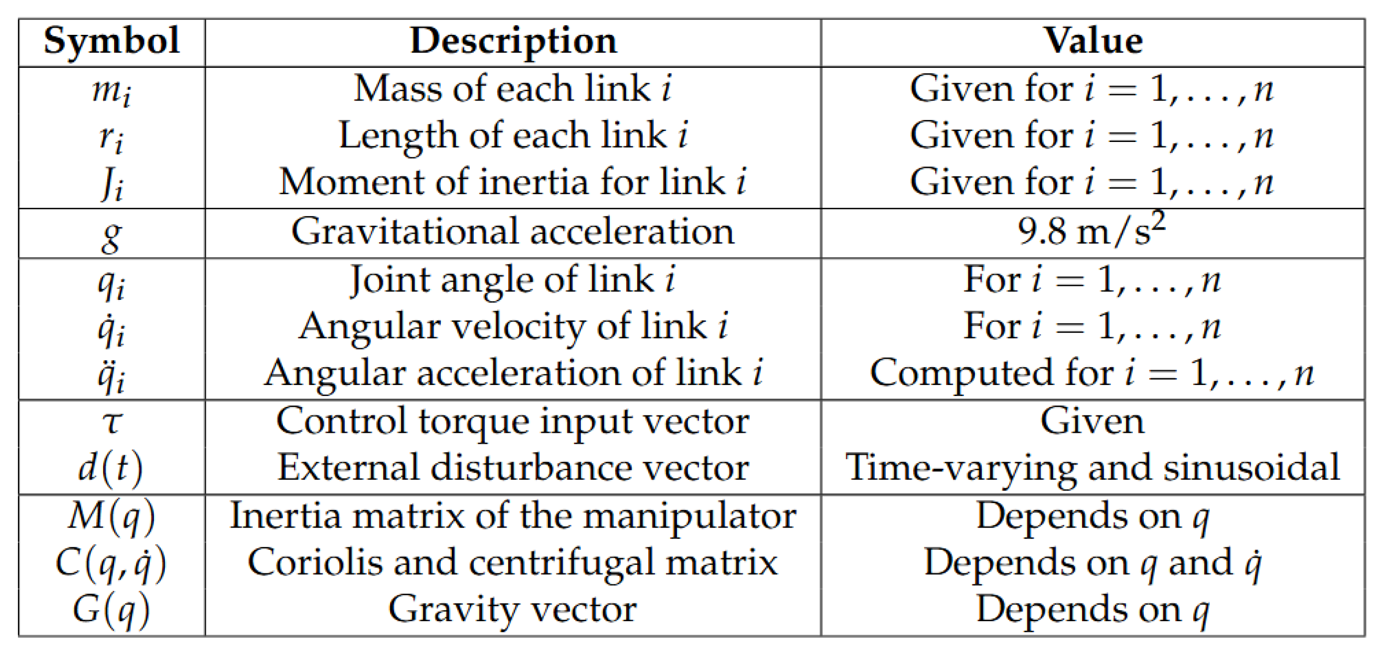
Figure 1 shows the parameters of an n-link manipulator.

First, a mathematical model is established for a series-connected multi-link robotic arm. The mass center of each link is positioned at half the length of the link:

$$l_i={\displaystyle \frac{r_i}{2}},i=\overline{1:n}$$

(1)

where $i=\overline{1:n}$ stands for $i=1,2,\dots ,n$.

The horizontal and vertical coordinates at the mass center of each connecting rod are formulated below:

$$\left[\begin{array}{c}x\\ y\end{array}\right]=\sum _{i=1}^n{\mathit{\ell }}_i\left[\begin{array}{c}cos\left({\displaystyle \sum _{j=1}^i{q}_j}\right)\\ sin\left({\displaystyle \sum _{j=1}^i{q}_j}\right)\end{array}\right],{\mathit{\ell }}_i=\left\{\begin{array}{cc}{r}_i,\hfill & i=\overline{1:n-1},\hfill \\ \frac{r_n}{2},\hfill & i=n.\hfill \end{array}\right.$$

(2)

The time derivatives of these coordinates, representing the velocities, are

$$\begin{array}{cc}\hfill {\dot{x}}_{c_i}& ={\displaystyle \frac{d}{dt}}\left(x_{c_i}\right),\hfill \end{array}$$

(3)

$$\begin{array}{cc}\hfill {\dot{y}}_{c_i}& ={\displaystyle \frac{d}{dt}}\left(y_{c_i}\right),i=\overline{1:n}\hfill \end{array}$$

(4)

Let the angular position ${\theta }_i$ of the i-th link equal the joint angle; therefore, ${\dot{\theta }}_i={\dot{q}}_i$, and the manipulator kinetic energy is defined as

$$K=\sum _{i=1}^n{\displaystyle \frac{1}{2}}{m}_i\left({\dot{x}}_i^2+{\dot{y}}_i^2\right)+{\displaystyle \frac{1}{2}}{J}_i{\dot{\theta }}_i^2$$

(5)

The manipulator potential energy is defined below:

$$P=-\sum _{i=1}^n{m}_{i}g{y}_i$$

(6)

Then, the corresponding Lagrangian energy function of the manipuator is defined as

$$L=K-P$$

(7)

The Lagrangian represents the difference between kinetic and potential energies and describes the dynamics of a physical system using energy functions instead of direct forces.

Expanding the Lagrange formulation results in an alternative manipulator motion equation [23]:

$$M\left(q\right)\ddot{q}+C(q,\dot{q})\dot{q}+G\left(q\right)=\tau +d$$

(8)

where bounded d represents the lumped disturbance term, including friction, payload variation, modelling uncertainty, and external interference. The above equation represents the general Newton’s law ruled motion of an n-link manipulator (Algorithm 1).

Algorithm 1 Newton motion equation ($M\left(q\right)$, $C(q,\dot{q})$, $G\left(q\right)$) by Lagrangian formulation [32]

Input:  q, $\dot{q}$, $m_i$, $r_i$, $J_i$, and g 1.  Define symbolic variables: $q_i$, ${\dot{q}}_i$, $m_i$, $J_i$, and g 2.  Compute the positions of the centers of mass: $$(x_i,y_i)\leftarrow \mathrm{obtained}\mathrm{from}\mathrm{forward}\mathrm{kinematics}$$ 3.  Determine linear velocities using the Jacobian: $$v_i={\displaystyle \frac{d}{dt}}{[x_i,y_i]}^T=J_{v_i}\left(q\right)\dot{q}$$ 4.  Calculate kinetic and potential energies: $$T=\sum _i\left(\frac{1}{2}{m}_i{\parallel v_i\parallel }^2+\frac{1}{2}{J}_i{\dot{q}}_i^2\right),V=\sum _i{m}_{i}g{y}_i$$ 5.  Define the Lagrangian:  $L=T-V$ 6.  Apply the Lagrange equation of motion: $${\displaystyle \frac{d}{dt}}\left({\displaystyle \frac{𝜕L}{𝜕{\dot{q}}_i}}\right)-{\displaystyle \frac{𝜕L}{𝜕q_i}}={\tau }_i$$ 7.  Derive the dynamic matrices: $M\left(q\right)={\displaystyle \frac{{𝜕}^{2}L}{𝜕{\dot{q}}_i𝜕{\dot{q}}_j}}$                             (Inertia matrix) $G\left(q\right)={\displaystyle \frac{𝜕V}{𝜕q_i}}$                              (Gravity vector) ${\mathbf{C}}_{ijk}={\displaystyle \frac{1}{2}}\left({\displaystyle \frac{𝜕M_{ij}}{𝜕q_k}}+{\displaystyle \frac{𝜕M_{ik}}{𝜕q_j}}-{\displaystyle \frac{𝜕M_{jk}}{𝜕q_i}}\right)$                            (Coriolis/centrifugal coefficients) Output:  The matrices $M\left(q\right)$, $C(q,\dot{q})$, and $G\left(q\right)$ satisfy: $$M\left(q\right)\ddot{q}+C(q,\dot{q})\dot{q}+G\left(q\right)=\tau$$

Figure 1. Dynamic parameters of the n-link manipulator [33,34].

Figure 1. Dynamic parameters of the n-link manipulator [33,34].

3. Data-Driven Model-Free Terminal Sliding Mode Control

3.1. Control Objectives and Assumptions

The major objectives of the data-driven model-free sliding mode control include (1) specifying the sliding mode surface and determining the controller, (2) analysing boundedness while the total uncertainty is treated as a bounded disturbance, (3) analysing reachability in relation to the stabilisation and convergence, and (4) providing the analytical assurances to simulation demonstrations and applications.

Definition 1. 

Data-driven model-free controller $\tau \left(t\right)$ for a given n-link manipulator: The controller output is generated using only measured data ($q,\dot{q},q_{\mathit{iref}},{\dot{q}}_{\mathit{iref}}$) and does not require explicit knowledge of the plant model $M\left(q\right)$, $C(q,\dot{q})$, $G\left(q\right)$, and the associated parameters. Formally, at time t, the physical model is employed exclusively as the ground truth of the plant and does not participate in the controller synthesis.

$$\tau \left(t\right)=K_t\left(I\left(t\right)\right)$$

(9)

where information set $I\left(t\right)=\left\{q,\dot{q},q_{\mathit{iref}},{\dot{q}}_{\mathit{iref}}\right\}\in {\mathbb{R}}^{4n}$.

Assumption 1. 

The link stage number n is known for control system design. The manipulator is controllable and observable.

Assumption 2. 

The manipulator dynamics, including inertial coupling, Coriolis and centrifugal effects, gravitational forces, friction, parametric uncertainties, and external disturbances, are treated as an aggregated unknown term. This total lumped uncertainty is assumed to be bounded. $\parallel \Delta \left(t\right)\parallel \le \overline{\Delta },\overline{\Delta }>0$. It is not necessary to know the exact value of the bound $\overline{\Delta }$.

Assumption 3. 

Each joint is fully actuated, and the control input enters the system through a nonsingular input channel. The actuator dynamics are sufficiently fast such that control torques can be applied as designed. This ensures that finite-time convergence is not obstructed by actuator limitations.

Assumption 4. 

The initial joint positions and velocities are finite, $q\left(0\right),\dot{q}\left(0\right)\in {\mathbb{R}}^n.$ Therefore, no restriction is imposed on proximity to the equilibrium.

3.2. SMC Algorithm and Stability Analysis

Lemma 1. 

Suppose that Assumptions 1–4 hold. Then there exists a data-driven, model-free terminal sliding mode control law constructed using measurable system signals only, such that the closed-loop dynamics of the n-link robotic manipulator are finite-time-stable. That is, the joint tracking errors converge to zero in finite time, and all internal signals of the closed-loop system remain bounded.

Proposition 1. 

It is noted that this type of dynamically interconnected manipulators has no input–output coupling; accordingly, the multi-input and multi-output (MIMO) plants can be treated as n single-input and single-output (SISO) systems in terms of data-driven model-free control [35]; then, the corresponding SMs and controllers are formulated as the diagonal elements in the forms of $s=diag\{s_1,s_2,\dots ,s_n\}$ and $\tau =diag\{{\tau }_1,{\tau }_2,\dots ,{\tau }_n\}$.

To design the controller, define each of the joint tracking error terms as

$$e_i=q_i-q_{\mathit{i}\mathrm{ref}},{\dot{e}}_i={\dot{q}}_i-{\dot{q}}_{\mathit{i}\mathrm{ref}}$$

(10)

To improve convergence speed and enhance overall control performance, this study adopts a fast terminal sliding mode control (TSMC) strategy for controller design [27,30]. Define the sliding model manifold (SMM) as

$$s_i={\dot{e}}_i+\alpha e_i+{\lambda }_i\mathrm{sign}\left(e_i\right){\left|e_i\right|}^{q/p}$$

(11)

When $s=0$, the following relationship holds:

$${\dot{e}}_i=-\alpha e_i-{\lambda }_i\mathrm{sign}\left(e_i\right){\left|e_i\right|}^{q/p}$$

(12)

With a proper choice of the parameter $\lambda$, the system can reach the sliding surface $s=0$ in finite time, and it converges faster than conventional asymptotic sliding mode controls [30].

To analyse the system stability, define a series of Lyapunov function candidates as

$$V_i={\displaystyle \frac{1}{2}}{s}_i^2,i=\overline{1:n}$$

(13)

The corresponding time derivatives are

$$\dot{V_i}=s_i·{\dot{s}}_i$$

(14)

Since the sign function satisfies $\mathrm{sign}\left(e_i\right)={\displaystyle \frac{e_i}{|e_i|}}$ for $e_i\ne 0$, the nonlinear term $\mathrm{sign}\left(e_i\right){\left|e_i\right|}^{\frac{q}{p}}$ can be equivalently expressed as $e_i{\left|e_i\right|}^{\frac{q}{p}-1}$. The temporal evolution of the sliding surface can be rewritten as

$${\dot{s}}_i={\ddot{e}}_i+\alpha {\dot{e}}_i+{\lambda }_i{\displaystyle \frac{d}{dt}}\left(e_i{\left|e_i\right|}^{\frac{q}{p}-1}\right)$$

(15)

Considering the derivative of the nonlinear function, we obtain the following equivalent form:

$${\displaystyle \frac{d}{dt}}\left(e_i{\left|e_i\right|}^{\frac{q}{p}-1}\right)={\displaystyle \frac{q}{p}}{\left|e_i\right|}^{\frac{q}{p}-2}{e}_i{\dot{e}}_i$$

(16)

Hence, the time derivative is given below:

$${\dot{s}}_i={\ddot{e}}_i+\left(\alpha +{\lambda }_i\frac{q}{p}{\left|e_i\right|}^{\frac{q}{p}-2}{e}_i\right){\dot{e}}_i$$

(17)

By substituting this expression into the Lyapunov derivative $\dot{V_i}$, we obtain

$$\dot{V_i}=s_i\left[{\ddot{e}}_i+\left(\alpha +{\lambda }_i\frac{q}{p}{\left|e_i\right|}^{\frac{q}{p}-2}{e}_i\right){\dot{e}}_i\right]$$

(18)

To remove chattering and ensure smooth control, select a continuous sliding mode control, rather than switching the sliding mode control (the root of chattering effect), which is realised with a hyperbolic tangent function. Accordingly, the data-driven model-free controller is formulated as

$${\tau }_i={\dot{s}}_i=-K_i·tanh\left({\displaystyle \frac{s_i}{{\varphi }_i}}\right)$$

(19)

So, we have

$${\ddot{e}}_i=-\alpha {\dot{e}}_i-{\lambda }_i{\displaystyle \frac{q}{p}}{\left|e_i\right|}^{\frac{q}{p}-i}{\dot{e}}_i-K_{i}tanh\left(\frac{s_i}{{\varphi }_i}\right)$$

(20)

where

• $K_i>\overline{\Delta }$: Control gain, and $\overline{\Delta }(M,C,G,d)$ is the total uncertainty bound;
• ${\varphi }_i>0$: Parameter adjusting the smoothness of tanh, consequently tuning the Lyapunov stability direction gradient on the sliding mode manifold plane $\left(s_i{\dot{s}}_i\right)$ [27].

Corollary 1. 

The controller (19) has two roles to hold the Lyapunov stability ${\dot{V}}_i={\dot{s}}_i{s}_i\le 0$. The gain $K_i$ represents the strength to suppress the uncertainty while the hyperbolic tangent function $tanh\left({\displaystyle \frac{s_i}{{\varphi }_i}}\right)$ is a strictly monotone function with respect to $s_i$. Together, they ensure that the Lyapunov derivative strictly decreases on the sliding mode manifold plane, yielding smooth convergence $\left(s_i{\dot{s}}_i\right)$ [27].

Since the hyperbolic tangent function satisfies the inequality

$$s_i·tanh\left({\displaystyle \frac{s_i}{{\varphi }_i}}\right)\ge 0,\forall s_i,i=\overline{1:n}$$

(21)

The time derivative of the Lyapunov function satisfies

$${\dot{V}}_i={\dot{s}}_i{s}_i\le 0⟶\dot{V}=\sum _{i=1}^n{\dot{V}}_i\le 0$$

(22)

The Lyapunov function derivative $\dot{V}\le 0$ suggests that the system energy does not increase with time and thus the control law dissipates energy from the closed-loop system. Furthermore, when $\dot{V}=0$, the system states stay on the sliding surface. By invoking the finite-time stability properties, the trajectories rapidly converge to the sliding manifold within a finite time and remain there after reaching it. Therefore, the system is not only finite-time Lyapunov-stable but also finite-time-convergent to the sliding surface. This confirms the strong robustness of the designed control systems.

Remark 1. 

The data-driven model-free TSMC is (1) simpler because of the use of a basic TSM and a simple controller, satisfying the Lyapunov differential inequality, and, consequently, the singularity does not exist in the design. Additionally, it is (2) more robust because this is a type of total robust control, whereby the solutions are feasible within a relatively large domain rather than those in the neighbourhood of the nominal model-based solutions. This study expands the SISO formulation [27] into decentralised MIMO manipulator systems where the embedded research insight has been to provide concise/simple solutions to complex problems with proper academic analysis and computational experiments. Furthermore, (3) the approach is closer to the scenario in real system tuning and operation maintenance. It should be stressed that the new approach is considered as a supplementary reference and not a replacement to both model-based and adaptive approaches [22].

3.3. Boundedness Analysis (Upper Disturbance Limit)

Moving onto Lyapunov stability analysis, the system also needs to take into account the limitations of its performance under disturbances. The following analyses the bounded interference $d$ to the system Equation (8). For bounded d, there exists a constant $d_{max}$ such that

$$\parallel d_i\parallel \le d_{max},i=\overline{1:n}$$

(23)

Consider the structured closed-loop system below:

$$M\left(q\right)\ddot{q}+C(q,\dot{q})\dot{q}+G\left(q\right)=\tau +d$$

(24)

where the control law vector $\tau ={[{\tau }_1\dots {\tau }_n]}^{\top }$ and ${\tau }_i=-K_{i}tanh(s_i/{\varphi }_i)$

With reference to Equation (13), define the whole Lyapunov candidate function as

$$V={\displaystyle \frac{1}{2}}{s}^{\top }s$$

(25)

The corresponding time derivative is

$$\dot{V}=s^{\top }\dot{s}$$

(26)

From the designed control, ${\tau }_i=s_{i}tanh(s_i/{\varphi }_i)\le 0$. Applying the Cauchy–Schwarz inequality gives

$$\dot{V}\le -K_{min}\parallel s\parallel tanh(\ast )+\parallel s\parallel \parallel d\parallel$$

(27)

where $tanh(\ast )={[tanh({\displaystyle \frac{\parallel s_1\parallel }{{\varphi }_1}})\dots tanh({\displaystyle \frac{\parallel s_n\parallel }{{\varphi }_n}})]}^{\top }$

Since $\parallel d\parallel \le d_{max}$, the control system achieves uniformly ultimately bounded (UUB). Specifically, there exists a bounded region such that

$$\parallel s\parallel \le {\varphi }_i{tanh}^{-1}\left({\displaystyle \frac{d_{max}}{K_{min}}}\right)$$

(28)

As long as $d_{max}<K_{min}$, the sliding variable $s\left(t\right)$ remains within a finite neighborhood, ensuring that both joint position $q\left(t\right)$ and velocity $\dot{q}\left(t\right)$ are bounded.

Therefore, under bounded external disturbances, all system states remain finite, and the control law guarantees finite-time convergence to a small vicinity of the sliding surface, achieving robust and stable control performance.

In conclusion, the above analysis confirms that the proposed sliding mode controller is not only Lyapunov-stable but also guarantees the boundedness of system states under bounded disturbances, providing a theoretical foundation for the robustness evaluation in the following simulation demonstrations.

3.4. Reachability Analysis

In the last section, we introduced the Lyapunov function for each subsystem:

$$V_i=\frac{1}{2}{s}_i^2.$$

(29)

Along the system trajectories, its derivative can be written as

$$\begin{array}{cc}\dot{V_i}& =s_i{\dot{s}}_i=-K_i{s}_{i}tanh\left({\displaystyle \frac{s_i}{{\varphi }_i}}\right).\hfill \end{array}$$

(30)

Since $tanh(·)$ is an odd function, we can write

$$s_{i}tanh\left({\displaystyle \frac{s_i}{{\varphi }_i}}\right)=\left|s_i\right|tanh\left({\displaystyle \frac{|s_i|}{{\varphi }_i}}\right).$$

(31)

For $x\ge 0$, the hyperbolic tangent satisfies

$$x-{\displaystyle \frac{x^3}{3}}\le tanh\left(x\right)\le 1.$$

(32)

The lower bound can be verified by defining $f\left(x\right)=tanh\left(x\right)-x+x^3/3$, which satisfies $f^{\prime }\left(x\right)=x^2-{tanh}^2\left(x\right)\ge 0$ and $f\left(0\right)=0$, hence $f\left(x\right)\ge 0$.

Substituting $x=|s_i|/{\varphi }_i$ into (32) and multiplying both sides by $|s_i|$, we obtain

$${\displaystyle \frac{|s_i{|}^2}{{\varphi }_i}}-{\displaystyle \frac{|s_i{|}^4}{3{\varphi }_i^3}}\le s_{i}tanh\left({\displaystyle \frac{s_i}{{\varphi }_i}}\right)\le \left|s_i\right|.$$

(33)

Substituting (33) into (30) yields

$$-K_i\left|s_i\right|\le \dot{V_i}\le -K_i\left({\displaystyle \frac{|s_i{|}^2}{{\varphi }_i}}-{\displaystyle \frac{|s_i{|}^4}{3{\varphi }_i^3}}\right).$$

(34)

For sufficiently large $|s_i|\ge {\varphi }_i$, inequality (34) ensures

$$\dot{V}\le -K_{i}tanh\left(i\right)\left|s_i\right|=-K_{i}tanh\left(i\right)\sqrt{2V},$$

(35)

which guarantees that trajectories reach the boundary layer $|s_i|\le {\varphi }_1$ in finite time. Inside the boundary layer ($|s_i|<{\varphi }_1$), the inequality reduces to

$$\dot{V_i}\le -{\displaystyle \frac{2K_i}{{\varphi }_i}}{V}_i+{\displaystyle \frac{4K_i}{3{\varphi }_i^3}}{V_i}^2,$$

(36)

Inside the boundary layer ($|s_i|<{\varphi }_i$), the dominantterm is $-{\displaystyle \frac{2K_i}{{\varphi }_i}}{V}_i$. Since $V_i$ is small, the quadratic term ${\displaystyle \frac{4K_i}{3{\varphi }_i^3}}{V_i}^2$ is of higher order and can be neglected, which shows that $V_i$ decays exponentially to zero as $t\to \infty$.

The above derivation demonstrates that the smooth reaching law ensures finite-time convergence to a boundary layer around the sliding surface, and exponential convergence to the origin thereafter. This satisfies the standard reachability condition in sliding mode control.

4. Simulated Case Studies

4.1. Simulation Platform

To reduce computational complexity, this simulation study selects a 3-link manipulator as the ground truth of the dynamic plant, with the parameters listed in Figure 2. It is worth mentioning that the data-driven and model-independent controllers are designed without referring to the model parameters.

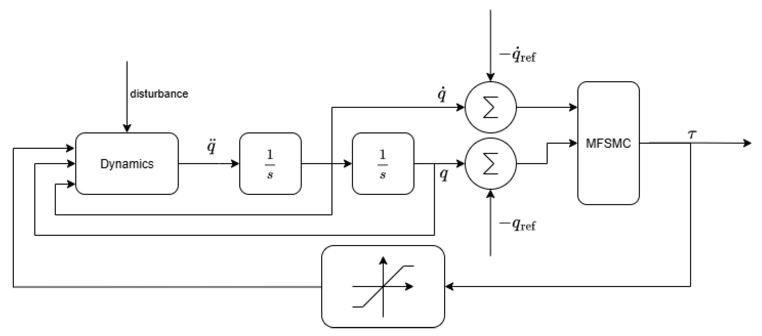
Figure 3 shows the whole closed-loop system structure. In Simulink R2024a, the most important module is four MATLAB Function modules (based on MATLAB R2024a). Among them, one MATLAB Function module is used to describe the system dynamics and is labeled as Dynamics to emulate the forward kinematics of the system. It accepts angular velocity, torque, and joint angle as its inputs and obtains the dynamic equations and results which are the angular acceleration of respective joints. The remaining three MATLAB Function modules are called the torque control modules and they respectively correspond to the three joints. In these modules, the joint angle and angular velocity are fed back and compared with the assigned trajectory signals to obtain the corresponding error vector. Subsequently, these error signals are used to construct the sliding surface and also the control torque for each joint in the simulated systems.

Figure 2. Dynamic parameters of the 3-link manipulator.

Figure 2. Dynamic parameters of the 3-link manipulator.

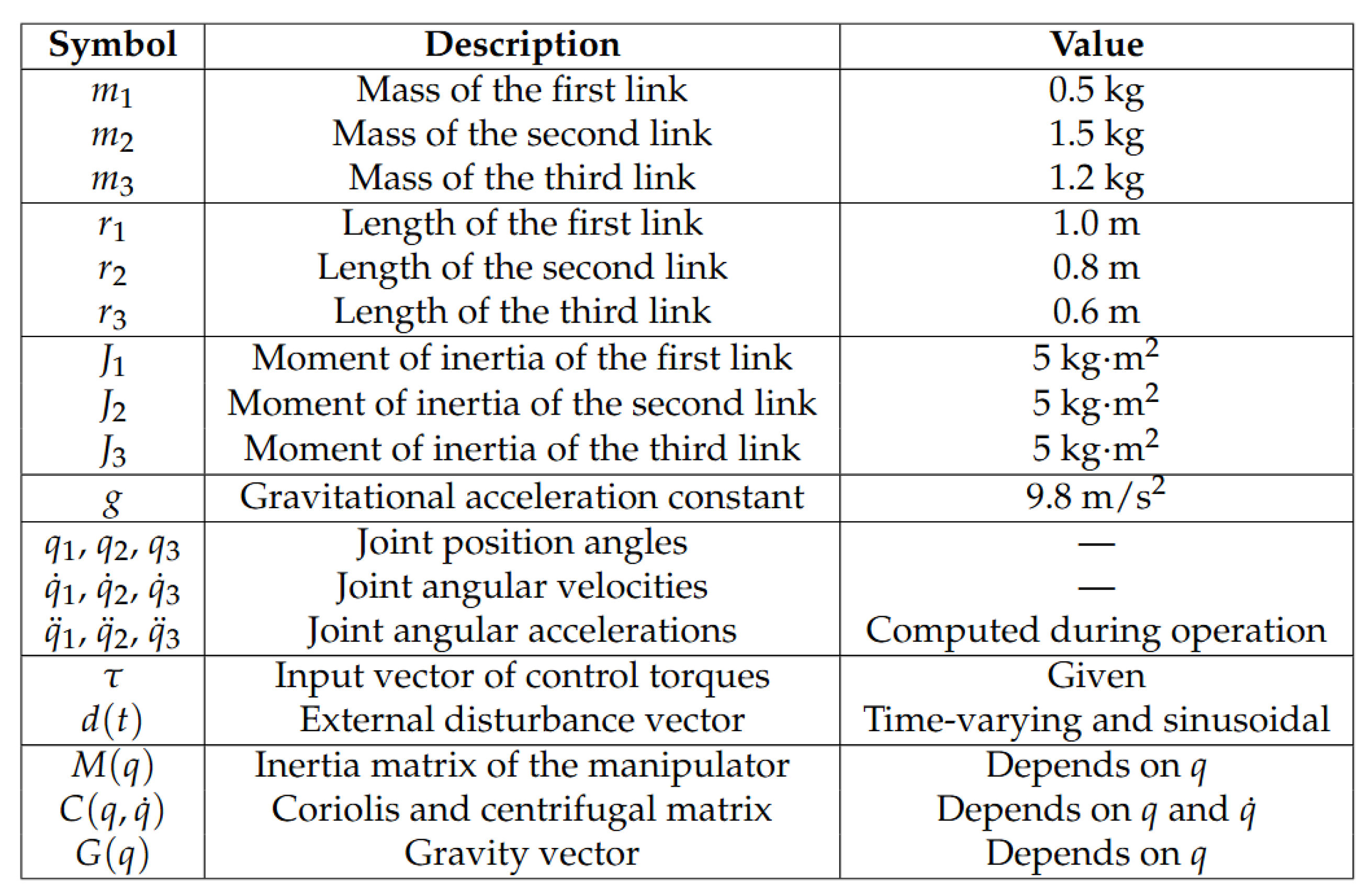
Figure 3. MFSMC control scheme diagram.

Figure 3. MFSMC control scheme diagram.

Each of the three control torques is defined as

$${\tau }_i=-K_{i}tanh\left({\displaystyle \frac{s_i}{{\varphi }_i}}\right)$$

(37)

4.2. Experimental Setup and Data Collection

The controlled plant is a planar 3-DOF manipulator that has a nonlinear coupling between the three joints. Each joint is driven by a sliding mode controller. The planned experimental demonstration objectives can be described as follows: (1) The dynamic and steady-state characteristics of the system are evaluated by tracking an exponential reference trajectory that contains rich dynamic characteristics. (2) Interference signals are added in the experiment as Equations (38)–(41) to test the robust stability of the control system in a more complicated and realistic environment. Multiple sets of experiments were conducted under different disturbance conditions to evaluate the response performance of the system in various situations. (3) To test the performance in dealing with system internal uncertainties, the next test is to change the controllable range of the load while the other parameters remain unchanged. (4) The initial joint positions in the experiment are set as $[0,1.58,2]\mathrm{rad}$. The experiment has used the following indicators to check the performance of the simulated system:

$$\begin{array}{cc}\hfill \mathrm{No}\mathrm{Disturbance}:{\mathit{\tau }}_d\left(t\right)& =\left[\begin{array}{c}0\\ 0\\ 0\end{array}\right]\hfill \end{array}$$

(38)

$$\begin{array}{cc}\hfill \mathrm{High}-\mathrm{frequency}\mathrm{Disturbance}:{\mathit{\tau }}_d\left(t\right)& =\left[\begin{array}{c}-0.5sin\left(200\pi t\right)\\ -0.5sin\left(200\pi t\right)\\ -0.4sin\left(200\pi t\right)\end{array}\right]\hfill \end{array}$$

(39)

$$\begin{array}{cc}\hfill \mathrm{Low}-\mathrm{frequency}\mathrm{Disturbance}:{\mathit{\tau }}_d\left(t\right)& =\left[\begin{array}{c}-2sint\\ -cos\left(2t\right)\\ -sin\left(3t\right)\end{array}\right]\hfill \end{array}$$

(40)

$$\begin{array}{cc}\hfill \mathrm{Mixed}\mathrm{Disturbance}:{\mathit{\tau }}_d\left(t\right)& =\left[\begin{array}{c}-2sint-0.5sin\left(200\pi t\right)\\ -cos\left(2t\right)-0.5sin\left(200\pi t\right)\\ -sin\left(3t\right)-0.4sin\left(200\pi t\right)\end{array}\right]\hfill \end{array}$$

(41)

• Steady-State Error (SSE): The steady-state error is the difference between the output and the setpoint after the system is converged, which has been used as the first indicator for almost all designed control systems.
• Mean Squared Error (MSE): The mean absolute value of the tracking error over all simulation time. This metric measures the average magnitude of the tracking error, that is, how far on average the system output deviates from the desired reference during the entire simulation. It focuses on accuracy rather than speed or stability alone.
• Maximum Error: The maximum instantaneous value of the error between the system response and the desired trajectory. This metric measures the worst-case tracking deviation between the system response and the desired trajectory. In simple terms, it tells how far the system output ever strays from the desired signal at any instant in time.
• Sliding Surface Reaching Time: The time taken to reach the sliding surface. This measures how quickly the system transitions from the reaching phase to the sliding phase, where the ideal robust control behaviour occurs.
• Control Torque Energy: This represents the energy consumed by the actuators (motors, servos, etc.) to achieve the desired tracking or motion. High control energy implies the system is working harder (more aggressive control). Low control energy means more efficient control (less actuator wear and power consumption).
• Estimated Convergence Time: This is used for indicating finite-time convergence.

4.3. Tracking Control

The MFTSMC parameters are as shown in Table 1 and their effects on the system are explained below:

Table 1. MFTSMC parameter settings for each joint.

Joint	$\mathit{\lambda }$	$\mathit{\alpha }$	K	$\mathit{\varphi }$	q	p
Joint 1	0.5	1	100	0.1	7	8
Joint 2	0.5	1	200	0.1	7	8
Joint 3	0.5	1	120	0.1	7	8

• $\lambda$ (Sliding Surface Proportional Coefficient):
  This coefficient is used to control the rate at which the system converges towards the sliding surface ($s=\dot{e}+\lambda e$), where $\dot{e}$ is the error rate and $\lambda$ is the adjustable parameter. When $\lambda$ increases, the system approaches the sliding surface more rapidly. If $\lambda$ is set too high, the system may experience overshoot or oscillation, resulting in an unstable response.
• $\alpha$ (Linear Error Gain Term): $\alpha$ is used to adjust the weight of the linear term in the sliding surface, as shown in Equation (11). By changing the value of $\alpha$, the transient response can be optimised, making the system perform more smoothly during the convergence process.
• K (Control Gain): The control gain K determines the system’s ability to resist external disturbances and acts to compensate for model uncertainties. A larger K leads to stronger suppression of disturbances and faster error correction. However, if K is too large, it may cause stronger oscillations.
• $\varphi$ (Chattering Suppression Coefficient): This parameter is used to reduce the high-frequency jitter in the control signal, usually achieved through the saturation function $\mathrm{sat}(s/\varphi )$. As the value of $\varphi$ increases, the switching action becomes smoother, which helps to enhance the overall stability of the system.
• q, p (Exponents): These nonlinear power exponents are essential components of the terminal sliding mode control (TSMC) design. They define how the fractional powers of the tracking error are calculated and therefore directly influence the degree of nonlinearity and the convergence rate of the control law. By selecting appropriate values of q and p, finite-time convergence can be achieved, and the robustness against uncertainties and disturbances can be improved.

4.3.1. Load Boundary

Experimental results indicate that the control gain K needs to be set to at least ${10}^2$ for the system to remain stable. If K is smaller than this value, the controller cannot keep the system stable, even when there are no external disturbances or extra payloads. This instability mainly happens because a small K does not provide enough control torque to balance the gravitational forces on the links.

Based on multiple simulation tests using the current parameter setup, the system can maintain full control performance when the external load is within the range of about $[0,11.21]\mathrm{kg}$. Since each of the three links, together with its actuator, weighs around $1\mathrm{kg}$, this load limit is reasonable and matches the physical design of the manipulator.

These results demonstrate that as long as the payload stays within a moderate proportion of the total link mass, the developed control can maintain stability and precise control functionalities. Hence, a controller effectively ensures robustness and accuracy under realistic load conditions.

4.3.2. Disturbance Supression

We selected a 6 kg payload from the verified control range to run the disturbance trials. And the desired motion trajectories and velocities for the three joints are predefined as Equations (42)–(44), and shown in Figure 4. The experiments demonstrate how well each joint tracks its corresponding reference trajectory.

$$\begin{array}{cccc}\hfill q_{1,\mathrm{ref}}\left(t\right)& =1.25-{\displaystyle \frac{7}{5}}{e}^{-t}+{\displaystyle \frac{7}{20}}{e}^{-4t},\hspace{1em}\hspace{1em}\hspace{1em}\hfill & \hfill {\dot{q}}_{1,\mathrm{ref}}\left(t\right)& ={\displaystyle \frac{7}{5}}{e}^{-t}-{\displaystyle \frac{7}{5}}{e}^{-4t}\hfill \end{array}$$

(42)

$$\begin{array}{cccc}\hfill q_{2,\mathrm{ref}}\left(t\right)& =1.25+e^{-t}-{\displaystyle \frac{1}{4}}{e}^{-4t},\hspace{1em}\hspace{1em}\hspace{1em}\hfill & \hfill {\dot{q}}_{2,\mathrm{ref}}\left(t\right)& =-e^{-t}+e^{-4t}\hfill \end{array}$$

(43)

$$\begin{array}{cccc}\hfill q_{3,\mathrm{ref}}\left(t\right)& =1.0+{\displaystyle \frac{1}{3}}{e}^{-t}+{\displaystyle \frac{1}{4}}{e}^{-4t},\hspace{1em}\hspace{1em}\hspace{1em}\hfill & \hfill {\dot{q}}_{3,\mathrm{ref}}\left(t\right)& =-{\displaystyle \frac{1}{3}}{e}^{-t}-e^{-4t}\hfill \end{array}$$

(44)

Four test scenarios were scanned: (1) Without the occurrence of any disturbance, (2) high-frequency, (3) low-frequency, and (4) mixed disturbance containing high- and low-frequency components. The figure depicts the trajectory tracking and joint torque response of every group of experiments. Each group of experiments’ trajectory tracking and joint torque response are shown within the figure.

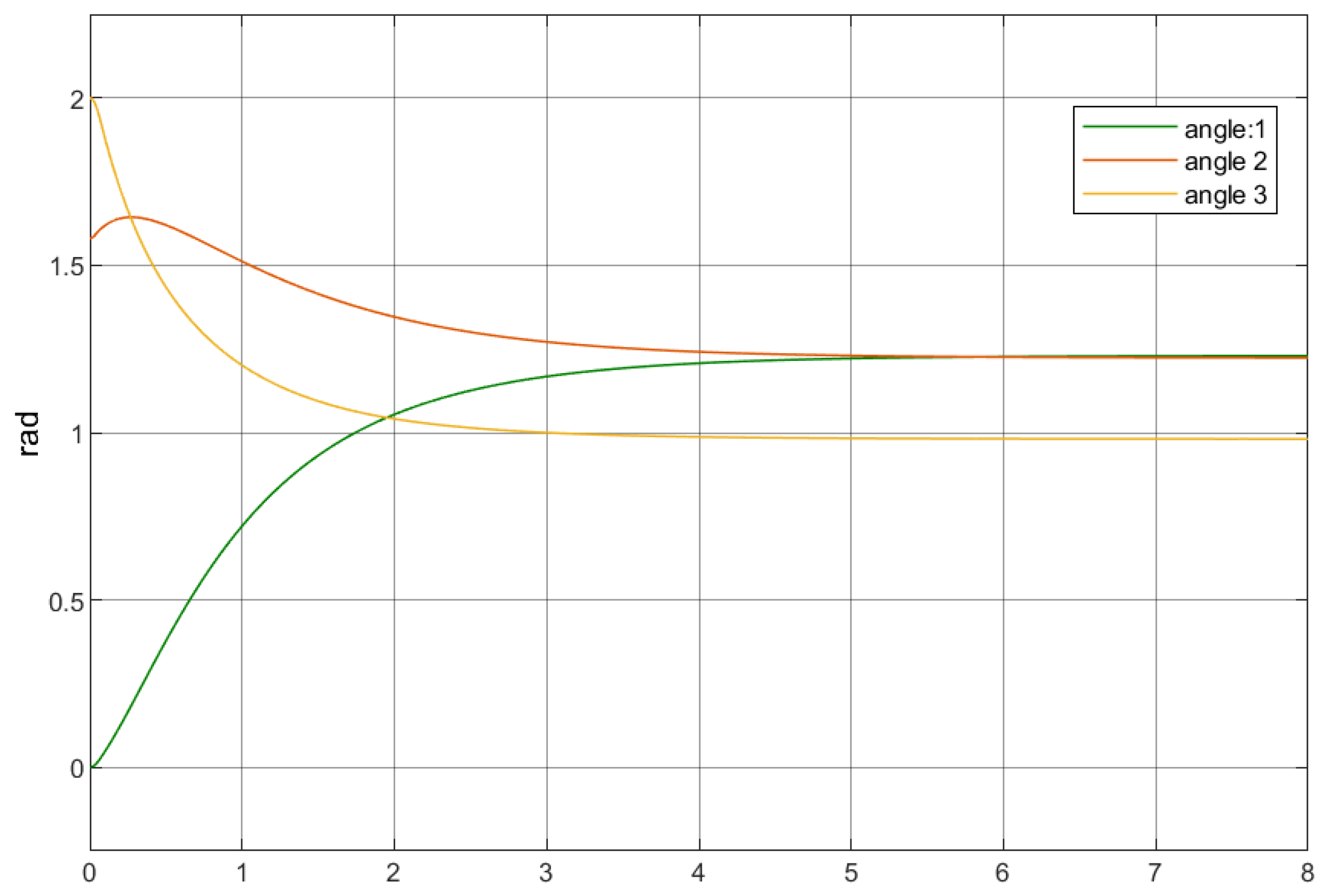
Comparing the motion trajectories in Figure 5, Figure 7, Figure 9 and Figure 11 demonstrates that external disturbances have only a small effect on the system performance. Each trajectory reaches its steady-state value in roughly 5 s, suggesting that the MFTSMC controller ensures high-level robustness and precise tracking of paths under all types of disturbances.

Figure 4. Reference trajectory profile.

Figure 4. Reference trajectory profile.

Figure 5. Joint angle response (no disturbance).

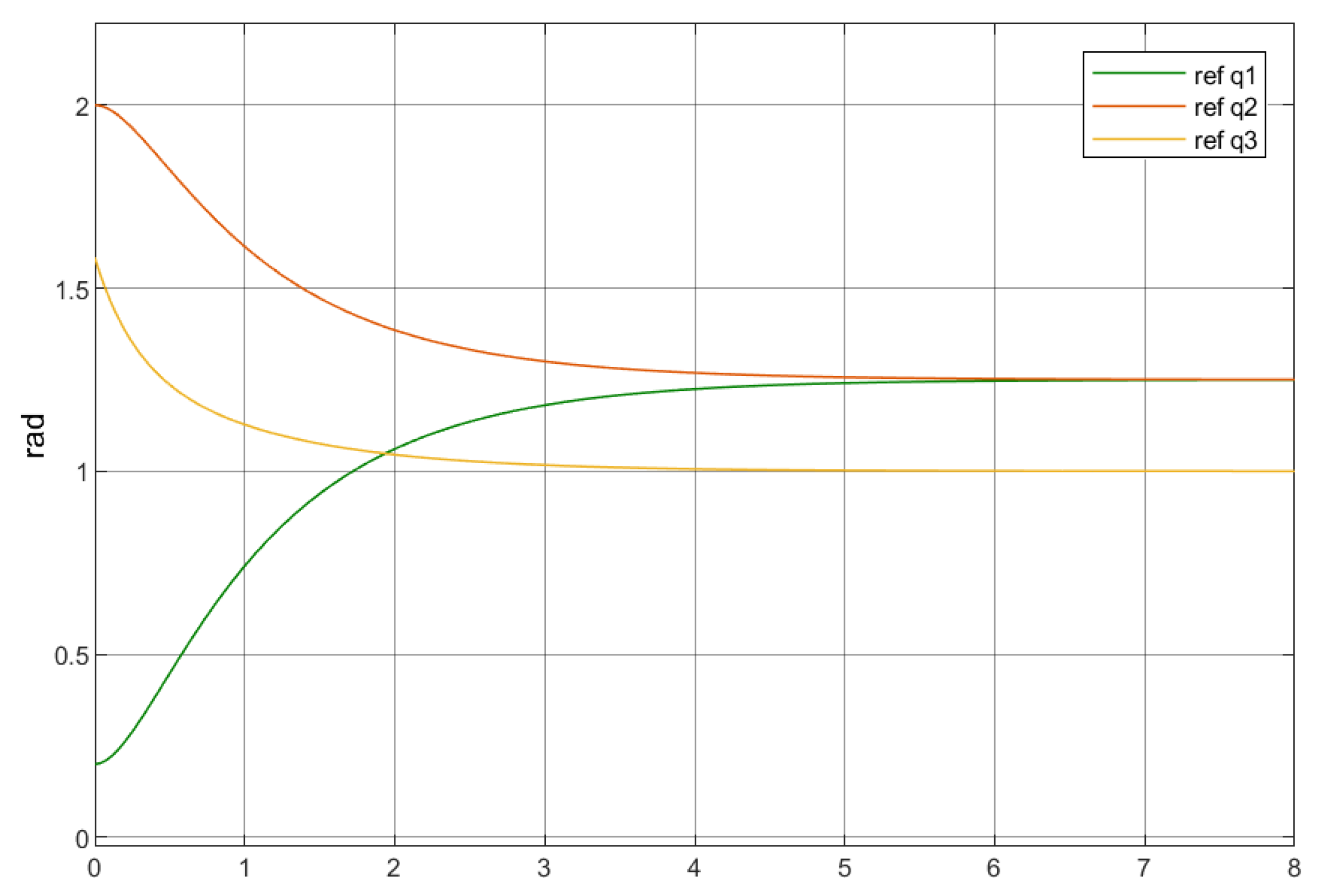
Figure 5. Joint angle response (no disturbance).

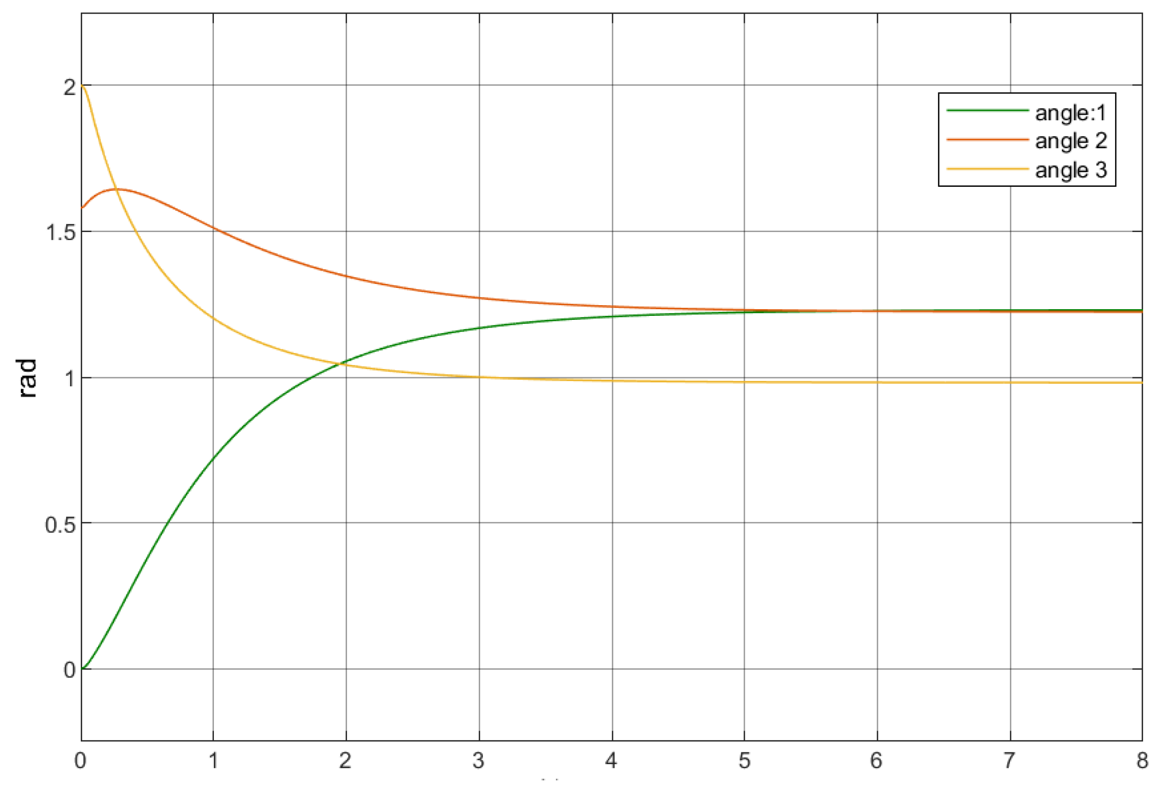
From the figure, all three joint trajectories exhibit smooth responses without noticeable overshoot and eventually converge to their respective steady-state values. Overall, the system demonstrates good stability.

Only Joint 2 shows a slight overshoot at the beginning of the response, reaching approximately $1.6\mathrm{rad}$, followed by a gradual decrease toward convergence. This indicates that the control gain of Joint 2 is slightly higher than that of Joints 1 and 3, although this does not compromise its stable behaviour.

The control torque under different disturbance conditions shows a consistent pattern. All three joints experience a large transient torque at the initial stage, and the magnitude of this transient response is influenced by the corresponding joint’s control gain K. The torques react quickly within the first 0–$0.5\mathrm{s}$, and after about 2–$3\mathrm{s}$, they enter a gradual stabilisation phase in which the torque variations progressively diminish. Eventually, each joint’s torque settles at a constant value or fluctuates slightly around a constant level, indicating that the system has fully converged and remains stably controlled.

Table 2 shows the convergence times measured under the different disturbance conditions.

Table 2. Convergence behaviour under multiple disturbances.

Disturbance Type	Convergence Time (s)
Without Disturbance	4.6
High-Frequency	5.0
Low-Frequency	7.4
Mixed Disturbance	6.9

Although the observed convergence times may appear somewhat unexpected, they can be explained as follows.

No-Disturbance Group (Figure 6): This group converges in 4.6 s. In the absence of external disturbances, the controller requires only small corrective actions, resulting in a relatively gentle response. Consequently, this group achieves the fastest convergence, and no noticeable torque fluctuations appear during the steady-state phase.

Figure 6. Control torque response (no disturbance).

Figure 6. Control torque response (no disturbance).

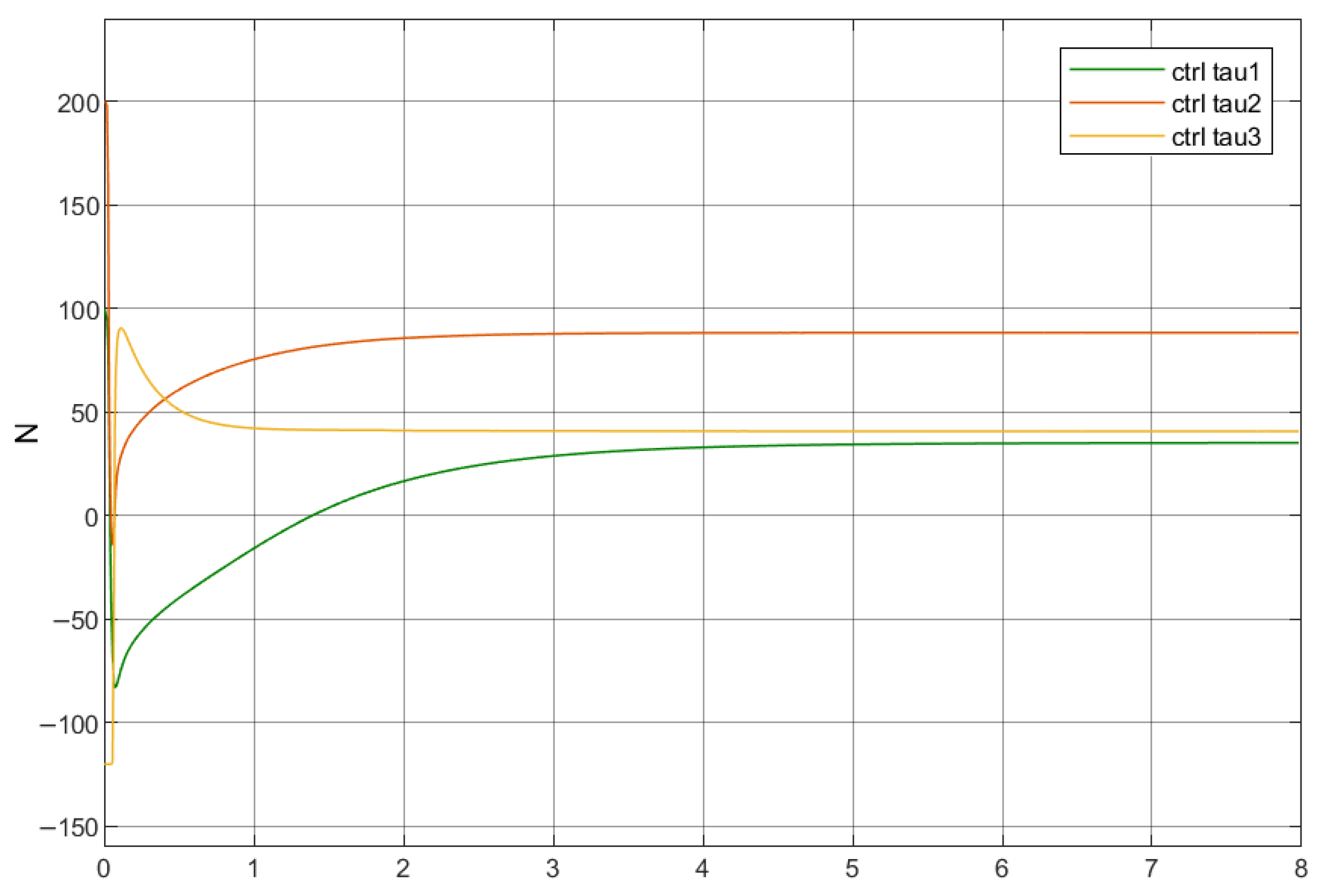
Figure 7. Joint angle response (high frequency only).

Figure 7. Joint angle response (high frequency only).

High-Frequency Disturbance Group (Figure 8): Under high-frequency disturbances, the convergence speed becomes slightly slower compared to the ideal no-disturbance condition, which uses 5.0 s. However, once reaching the steady state, the presence of high-frequency components causes small-amplitude oscillations of the control torque around its steady value, as the controller continuously counteracts the disturbance.

Figure 8. Control torque response (high frequency only).

Figure 8. Control torque response (high frequency only).

Figure 9. Joint angle response (low frequency only).

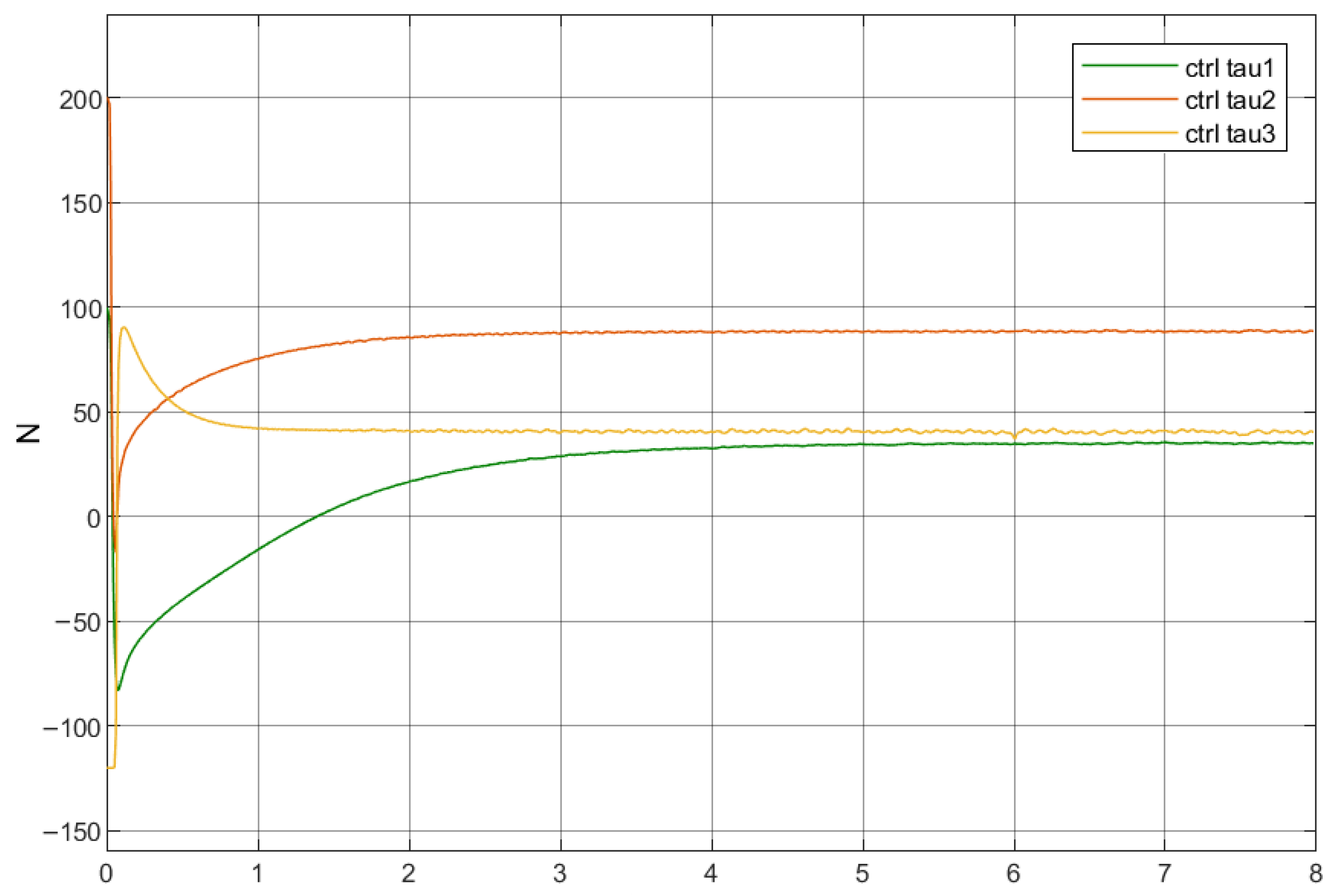
Figure 9. Joint angle response (low frequency only).

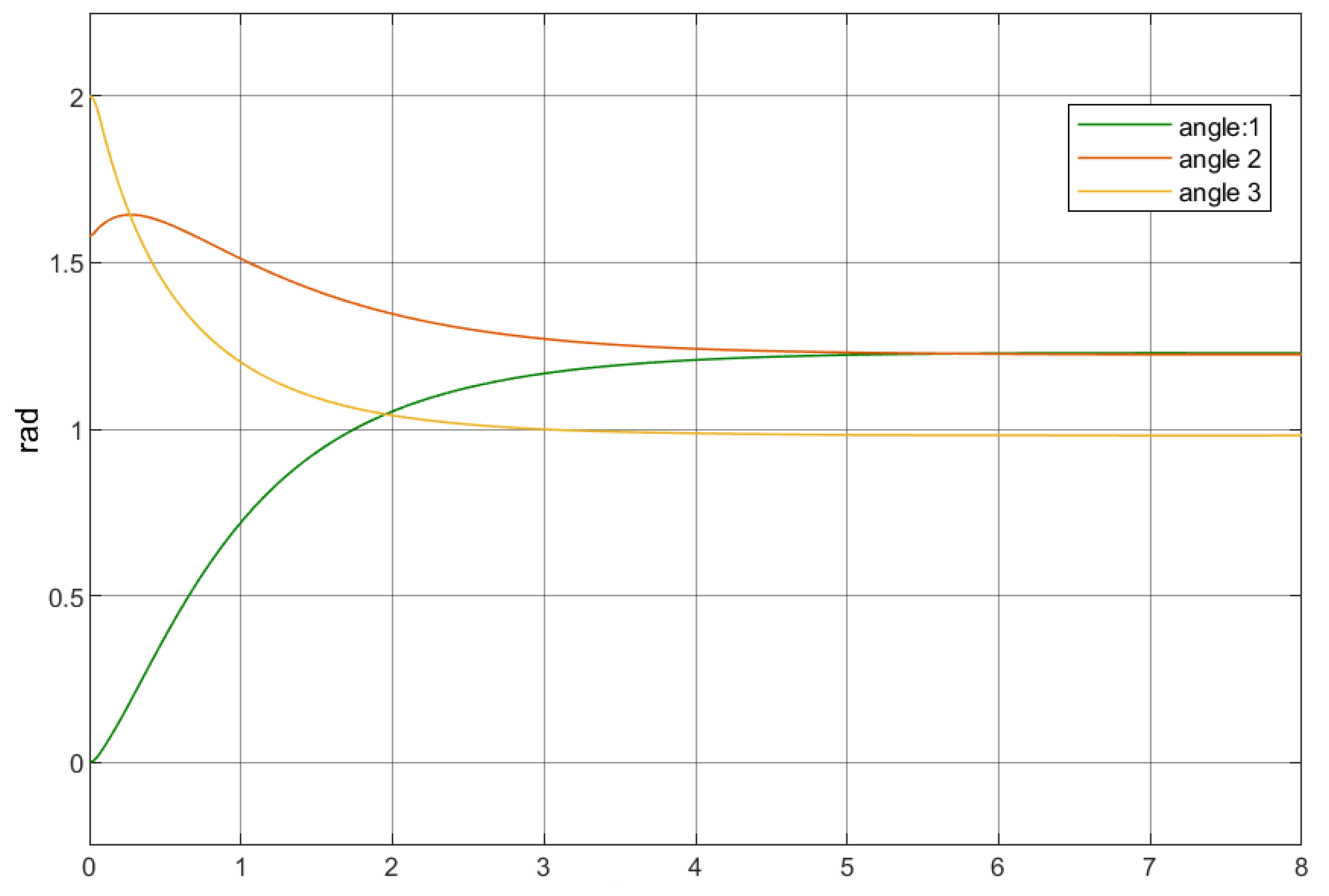
Low-Frequency Disturbance Group (Figure 10): This group converges in 7.4 s. Low-frequency signals typically induce phase delays and small residual oscillations. Because the controller reacts more slowly to such gradual disturbances, the convergence time of this group is significantly longer than in the other cases.

Mixed Disturbance Group (Figure 12): This group converges in 6.9 s. When both high- and low-frequency disturbances act simultaneously, the combined effects yield a convergence speed that lies between the high-frequency-only and low-frequency-only groups. Similar to the high-frequency group, small-amplitude torque oscillations also appear in the steady state.

Figure 10. Control torque response (low frequency only).

Figure 10. Control torque response (low frequency only).

Figure 11. Joint angle response (high + low frequency).

Figure 11. Joint angle response (high + low frequency).

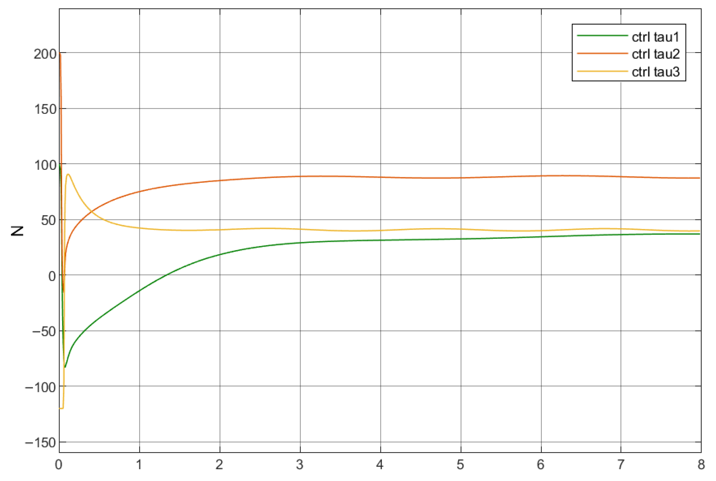
Figure 12. Control torque response (high + low frequency).

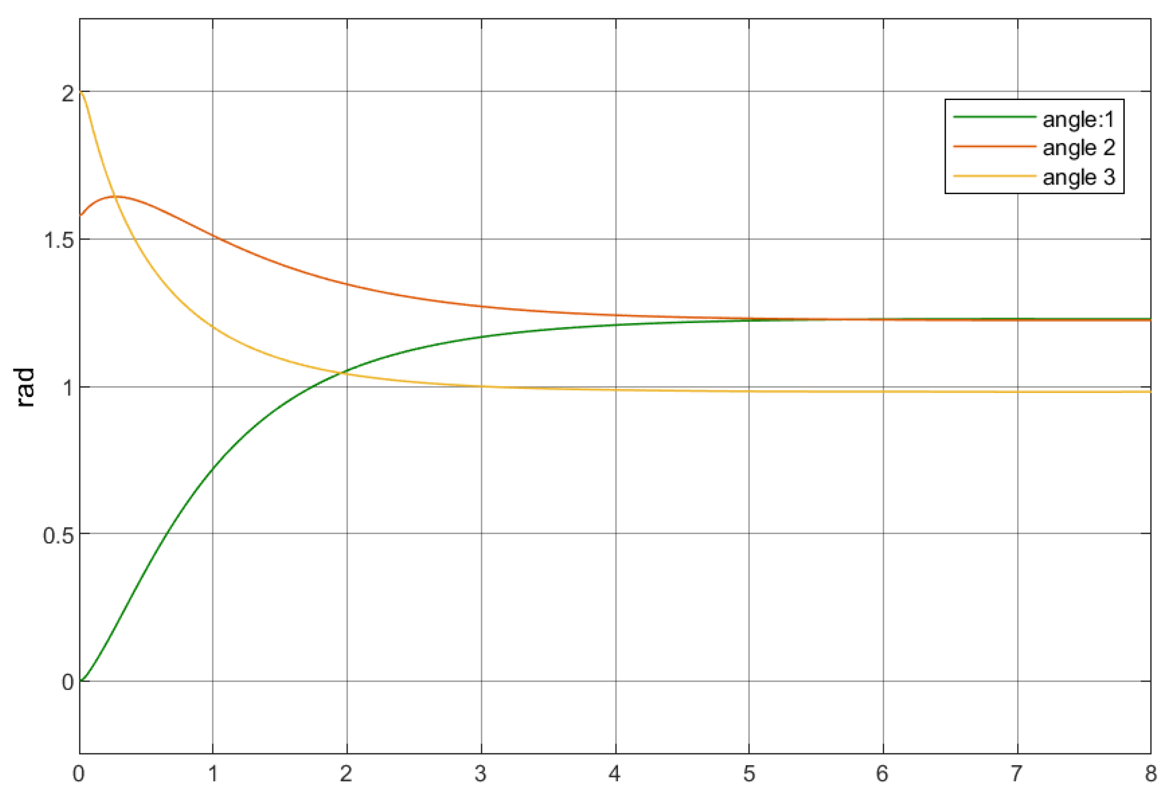
Figure 12. Control torque response (high + low frequency).

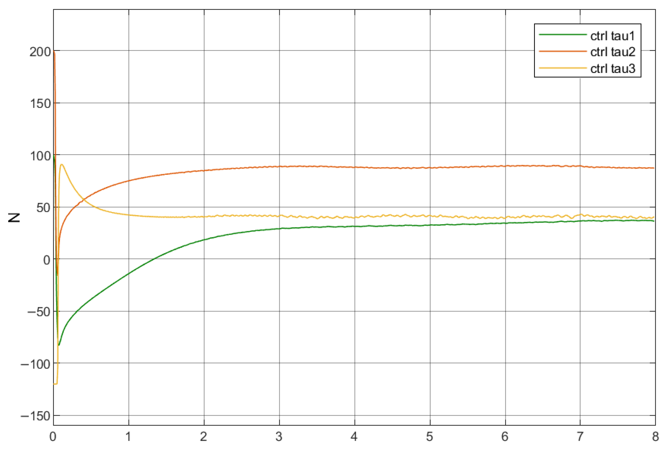
Therefore, it can be concluded that the dominating behaviour in the initial control response of all tests is the dynamic excitation, and that is why the reactions in the early stage are all similarly slightly strong. On the other hand, the convergence behaviour in mid and late stage depends on how well the controller can adapt to different disturbance frequencies. The most noteworthy result is that the mixed disturbance group demonstrates strong robustness and fast response. Since this type of disturbance is the most common in industrial environments, the result further confirms that the proposed control strategy has strong potential for practical engineering applications.

4.3.3. Assessment Indicators of Experimental Results

When the load is fixed at $6\mathrm{kg}$, mixed disturbances are added to the system to evaluate MFTSMC performance. The next four items are used to quantitatively analyse the transient response, steady-state precision, and energy consumption.

Steady-State Error (SSE)

The SSE is the gap between the system output and the assigned reference path after the transient response sessions. The average value of the output tracking error in the last period of the simulation is used to calculate this parameter.

$$e_{\mathrm{ss}}={\displaystyle \frac{1}{\Delta }}{\int }_{T-\Delta }^T\left|e\left(t\right)\right|dt$$

(45)

where

• $\Delta$: Time interval of the steady-state evaluation;
• T: Total simulation duration;
• $e\left(t\right)$: Instantaneous tracking error.

The computed steady-state errors are

Joint 1: $0.0205$; Joint 2: $0.0262$; and Joint 3: $0.0191$.

All joints converge with final errors on the order of ${10}^{-2}$ and effectively approach zero. This illustrates that the controller achieves the expected steady-state tracking precision and stability.

Mean Squared Error (MSE)

The MSE is used to measure the average energy of the tracking error over time in the form of

$$\mathrm{MSE}={\displaystyle \frac{1}{T}}{\int }_0^T{e}^2\left(t\right)dt$$

(46)

where $e\left(t\right)$ denotes the instantaneous tracking error and T represents the total simulation duration.

The calculated MSE numbers for each joint are

Joint 1: $0.0015$; Joint 2: $0.0084$; Joint 3: $0.0082$.

The error energy of Joint 1 is the smallest, while that of Joint 2 is the greatest. The differences among the three joints arise from the parameter variations of their respective controllers, and these differences do not affect system stability.

Maximum Error (ME)

Through numerical calculation, the maximum errors of the joints are, respectively,

Joint 1: $0.2000$; Joint 2: $0.4200$; Joint 3: $0.4428$.

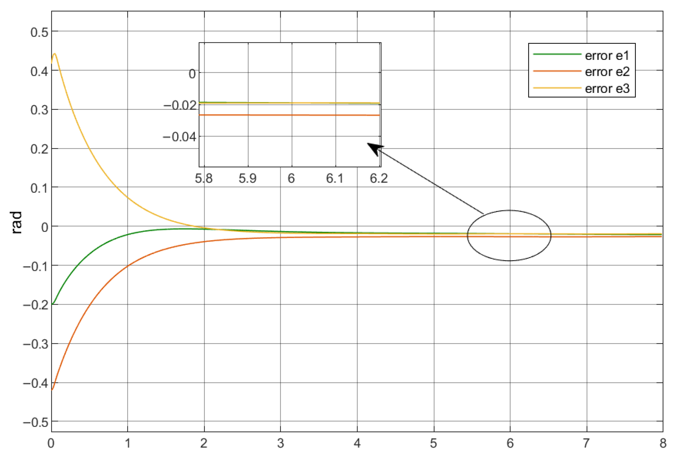
As shown in Figure 13, Joints 1–3 exhibit their maximum errors at the initial stage, after which the errors continuously decrease over time. The peak initial error reaches up to nearly $0.5,\mathrm{rad}$ but stabilises within 2 s. This phenomenon indicates that the controller is able to effectively track the desired trajectories of the joints.

Sliding Surface Reaching Time

The actual reaching time is defined as the moment when the system state first enters the vicinity of the sliding surface:

$$T_{\mathrm{reach}}=min\{t\mid |s\left(t\right)|\le ϵ\}$$

(47)

in which $s\left(t\right)$ denotes the sliding surface and $ϵ$ is a small threshold (e.g., $ϵ=0.01$) indicating the acceptable proximity to the surface.

By choosing a small threshold of $ϵ=0.02$, the reaching time of each joint can be recorded more clearly. Joint 1 and Joint 2 reach the sliding surface the quickest. Joint 3 needs the longest time. Even though the speeds are different, all joints complete the reaching process in less than 0.07 s. This shows the controller has a fast response for every joint.

When comparing the simulation results with the theoretical predictions, Joint 1 and Joint 3 match the expected behaviour. Joint 2 shows small deviations. These deviations mainly come from the initial overshoot. The differences are small, so the effectiveness and accuracy of the TSMC controller can still be supported.

Figure 13. Mixed disturbance tracking error response.

Figure 13. Mixed disturbance tracking error response.

Control Torque Energy

The control moment energy represents the total consumed energy by the actuator throughout the whole control process. By integrating the square of the control moment over the simulation period, the assessment of the overall system energy efficiency can be calculated by

$$E_{\tau }={\int }_0^T{\tau }^2\left(t\right)dt$$

(48)

where $\tau \left(t\right)$ is the control torque at time t.

The calculated energy consumption for each joint is illustrated below $({\mathrm{N}·\mathrm{m}}^2·\mathrm{s})$:

$$E_{{\tau }_1}=8.539\times {10}^3,E_{{\tau }_2}=5.7745\times {10}^4,E_{{\tau }_3}=1.5701\times {10}^4$$

These results indicate that there is a notable difference in energy consumption among the three joints. Joint 2 exhibits the highest energy usage, suggesting that it undertakes a greater portion of the compensatory effort associated with dynamic coupling. In contrast, Joint 1 shows the lowest energy consumption, which aligns with its smooth trajectory and the small error oscillations observed in the simulation.

Estimated Convergence Time (ECT)

For the given TSMC, the estimate of the upper bound of the sliding surface reaching time can be determined by [30]

$$T_{\mathrm{reach}}\le {\displaystyle \frac{p}{\lambda (p-q)}}{\left|e_0\right|}^{(p-q)/p}$$

(49)

where

• $e_0$: Initial tracking error;
• $p>q>0$: Order parameters;
• $\lambda$: Nonlinear coefficient in the sliding surface design.

The corresponding theoretical reaching times are

Joint 1: $1.3133\mathrm{s}$; Joint 2: $1.7670\mathrm{s}$; Joint 3: $1.7614\mathrm{s}$.

These represent ideal upper bounds under noise-free conditions. In practice, real reaching times are affected by external disturbances, integration errors, actuator saturation, and controller gain tuning, leading to slight deviations from the theoretical values. Thus, a comparison with actual measured reaching times is necessary for validation.

4.4. Model-Based TSMC Tests

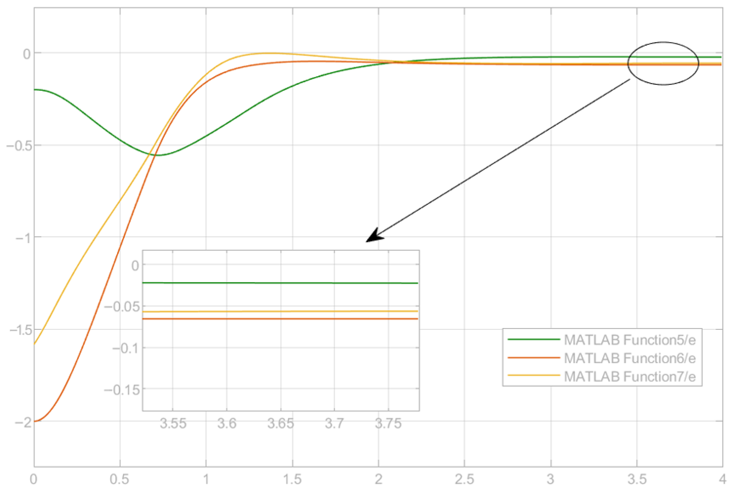
Appendix A presents the detailed control system design. Figure 14, Figure 15 and Figure 16 show the representative results of the MBTSMC simulation, including joint trajectories, control torques, and tracking errors. These results serve as the essential reference and foundation for the qualitative comparison and performance discussion conducted in the subsequent section.

Figure 14. Joint trajectory response q with MBTSMC.

Figure 14. Joint trajectory response q with MBTSMC.

Figure 15. Control torque $\tau$ with MBTSMC.

Figure 15. Control torque $\tau$ with MBTSMC.

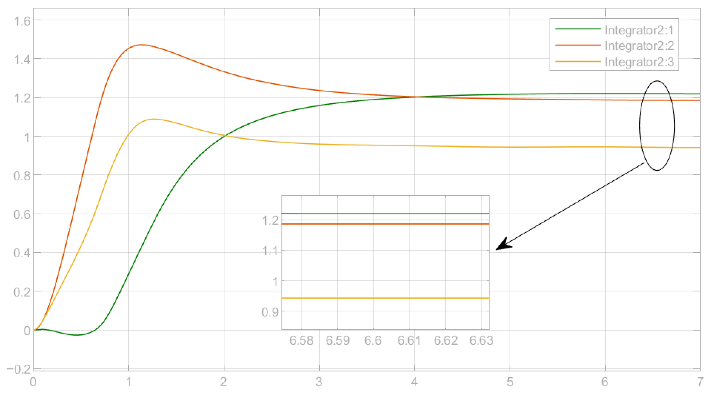
Figure 16. Tracking error with MBTSMC.

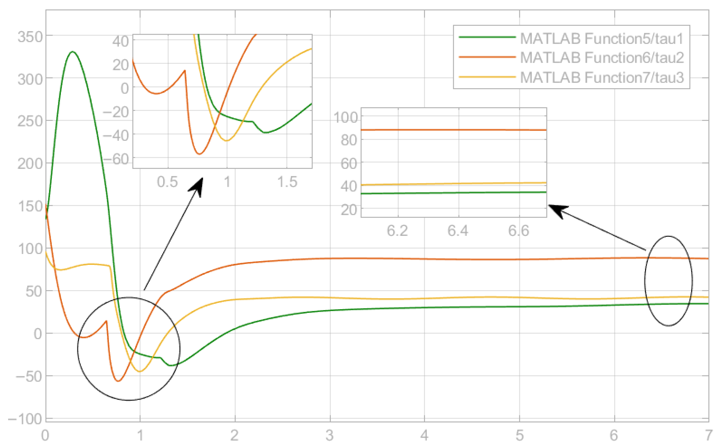
Figure 16. Tracking error with MBTSMC.

4.5. LQR Tests

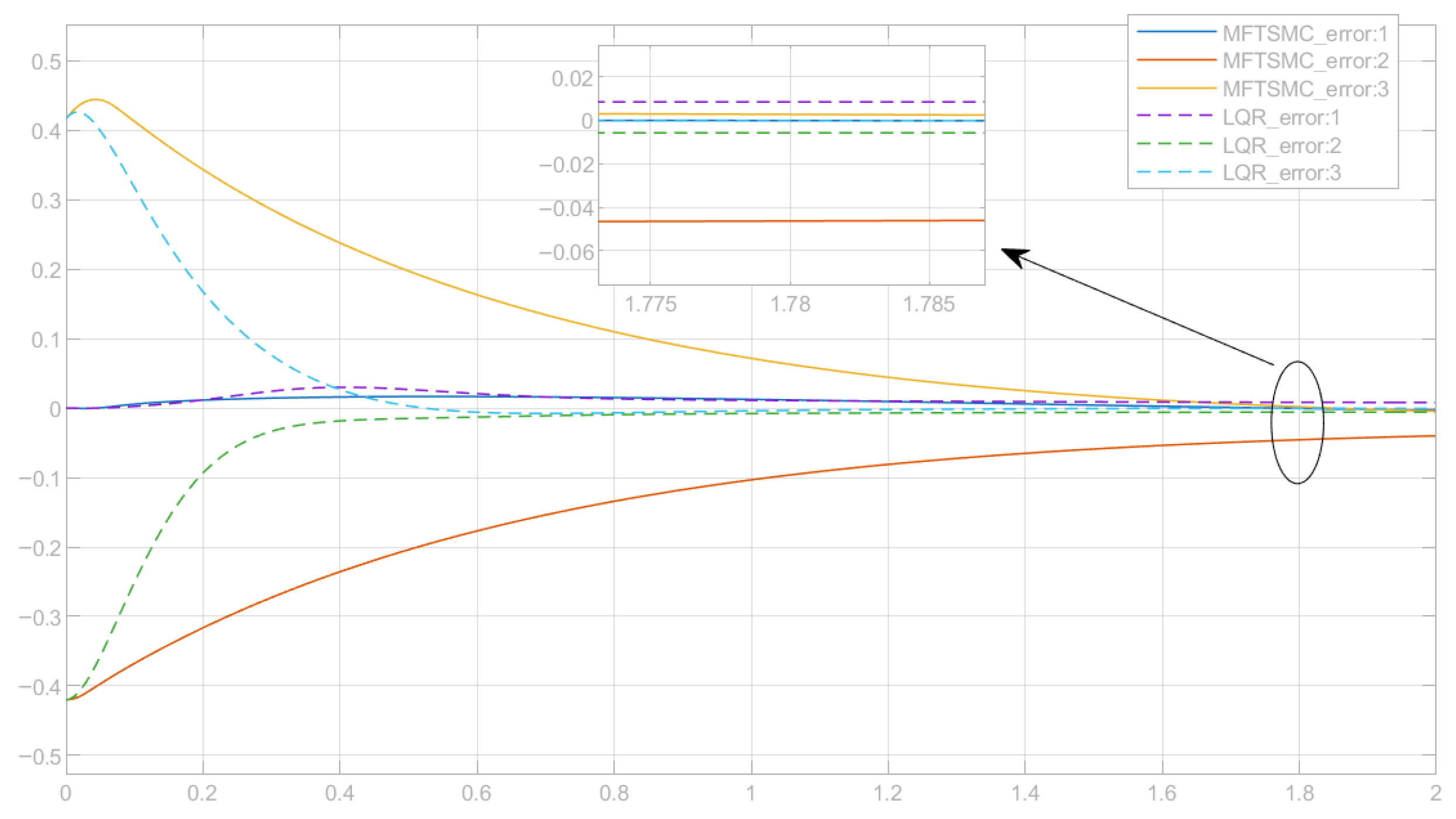
Figure 17, Figure 18 and Figure 19 show the representative simulation comparisons between the MFTSMC and LQR, including joint trajectories, control torques, and tracking errors. These results serve as the essential reference and foundation for the qualitative comparison and performance discussion conducted in the subsequent section.

Figure 17. Joint trajectory comparison between LQR and MFTSMC.

Figure 17. Joint trajectory comparison between LQR and MFTSMC.

Figure 18. Control torque comparison between LQR and MFTSMC.

Figure 18. Control torque comparison between LQR and MFTSMC.

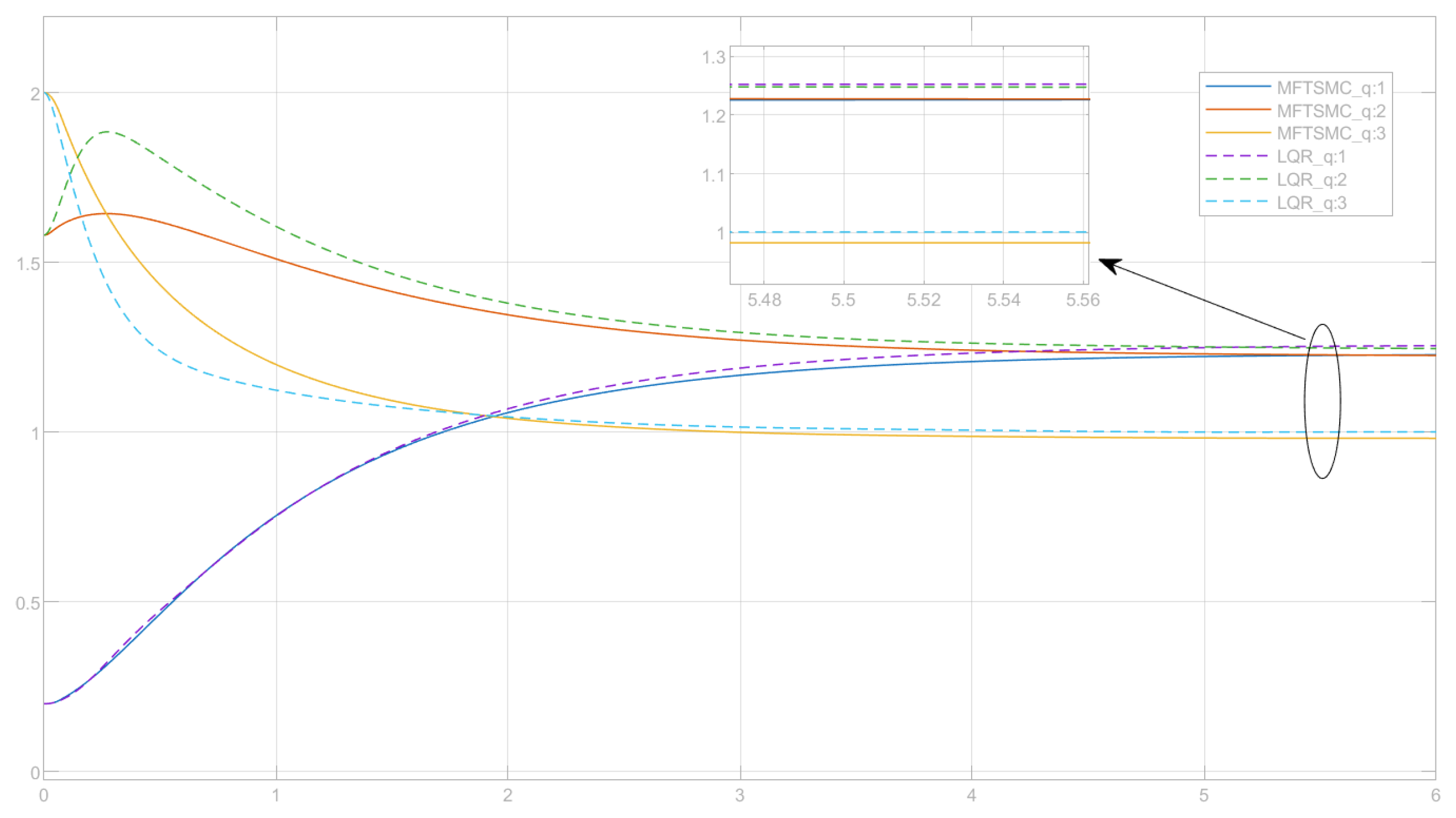
Figure 19. Tracking error comparison between LQR and MFTSMC.

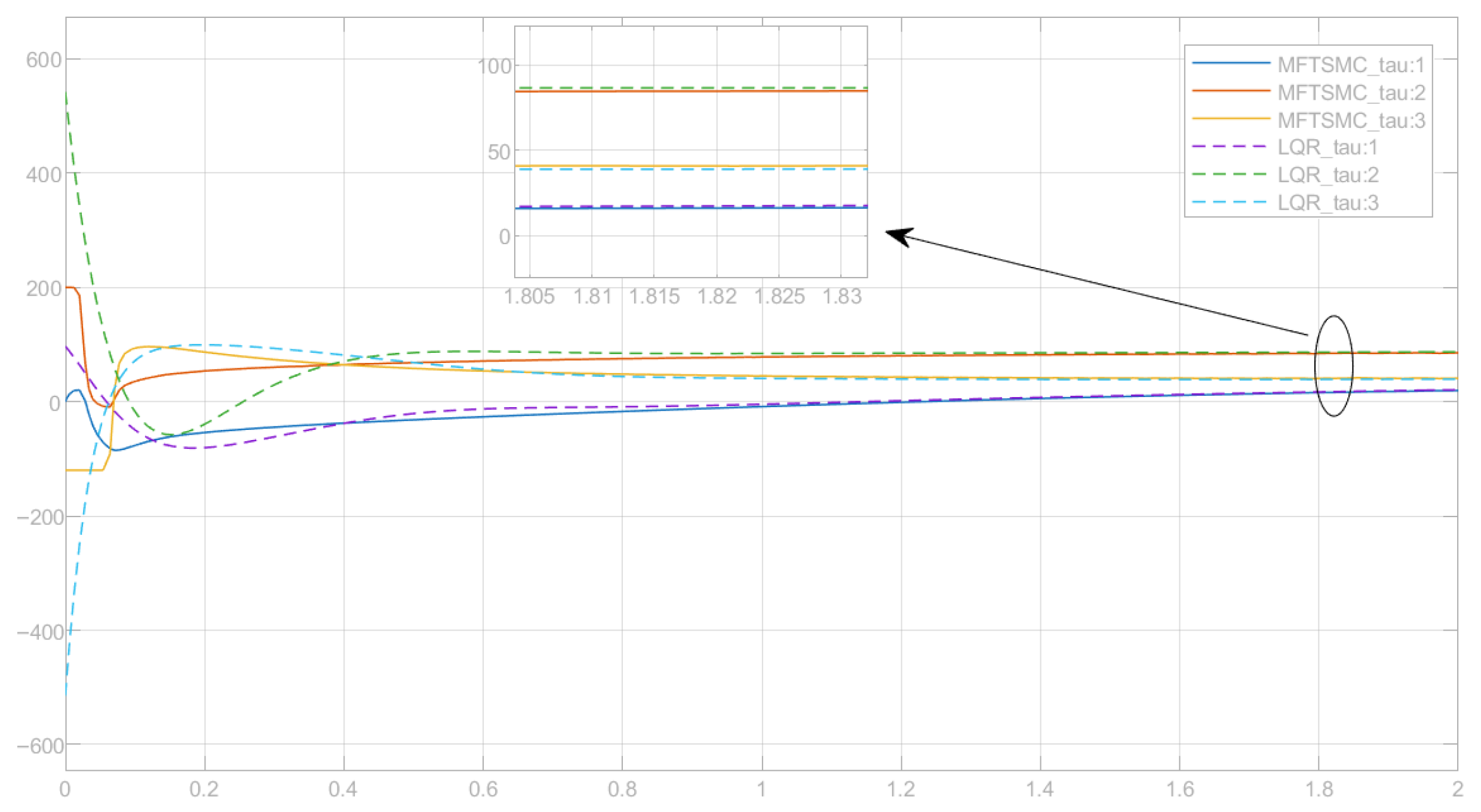
Figure 19. Tracking error comparison between LQR and MFTSMC.

4.6. General Discussions

The results from the previous sections indicate that, under the comprehensive evaluation of multiple parameters, MFTSMC can be regarded as having a good performance in handling such manipulator systems.

All joints move rapidly toward the sliding surface and reach the reference trajectory within a short period [36]. The maximum settling time is less than 0.07 s, demonstrating that the system exhibits a very fast transient response. Even in cases with noticeable initial overshoot, the trajectories quickly become smooth, indicating strong transient recovery capability and effective damping of oscillations.

The final tracking error stays within the order of ${10}^{-2}$ [37], which can be considered almost zero in practice. After the effect of external disturbance becomes small and the system reaches a steady state, the controller is able to consistently maintain a high tracking accuracy. Although this small steady-state error has minimal impact in practical applications, it can still be further optimised. By applying an integral sliding mode approach, the steady-state error can be completely eliminated [38]. Both theoretical analysis and experimental results show that MFTSMC provides excellent steady-state precision and reliable performance.

The results of the comprehensive analysis of the torque and energy indicate that, in the process of system operation, the system only consumes a relatively small control energy [39]. It means that the controller can make more reasonable use of energy and keep the process of motion continuous, which also meets the basic requirements of engineering applications.

Furthermore, when the system is subject to different kinds of external disturbances, for example, low-frequency interference, high-frequency interference, or the case of both, the system can still achieve stable convergence [40]. There is no divergence and instability in the control of torque, which means that the control strategy is still reliable in the face of complex situations. These results clearly show that the controller has strong robustness to imperfect models and unpredictable disturbances, and that it can maintain a stable performance even in complex dynamic environments.

Based on the previously presented results in Figure 14, Figure 15 and Figure 16, the control behaviour of the MBTSMC shows certain similarities to that of the MFTSMC. In the joint motion curves, Joints 2 and 3 exhibit only one overshoot, while Joint 1 also reaches the target smoothly.

In the tracking error e, MBTSMC converges slightly faster but still presents a small steady-state error. A similar trend is observed in the torque response $\tau$: MBTSMC enables all joints to reach steady torque within 3 s, but noticeable torque spikes appear, which may potentially reduce motor lifespan in physical implementations. By comparison, MFTSMC exhibits a smoother torque profile, with only transient sharp variations in the initial stage [41].

In addition to comparing MFTSMC with MBTSMC, this study also performs experiments to analyse the difference between MFTSMC and LQR [42]. To evaluate control performance, Figure 17, Figure 18 and Figure 19 present the results for a three-joint manipulator, including joint trajectories, tracking errors, and control torques. Both controllers achieve accurate trajectory tracking. However, clear differences can be observed in their dynamic responses and control energy usage.

The MFTSMC exhibits no noticeable overshoot across all three joints. This control behaviour reflects the finite-time convergence and nonlinear adaptive capability of terminal sliding mode control. In comparison, the LQR produces smoother trajectories with slight overshoot, while the convergence speed of the two controllers is similar, with no significant difference.

The proposed MFTSMC rapidly reduces the tracking error and brings it within the range of $\pm 5\times {10}^{-2}$ in approximately 2 s. The convergence process is fast and free of oscillations. By contrast, the LQR controller converges more quickly in the early stage, but its error curve is less smooth than that of the MFTSMC. Both controllers achieve comparable steady-state accuracy, with a steady-state error level of approximately $\pm 5\times {10}^{-2}$.

In terms of control torque, the MBTSMC produces noticeable fluctuations within the first 0.2 s, exhibiting the typical chattering characteristics of sliding mode control. After approximately 0.8 s, the torque becomes stable, and energy consumption is reduced accordingly. In contrast, the LQR generates torque signals with a larger initial magnitude, but with almost no high-frequency switching in the actuators. Under identical simulation conditions, MFTSMC provides shorter convergence time and stronger robustness, making it more suitable for nonlinear systems and disturbance-rich environments. The LQR consumes less energy and runs more smoothly, which is advantageous for systems with accurate models and stable external loads.

5. Conclusions

This control application-focused paper has proposed a data-driven, model-free terminal sliding mode control framework for multi-link robotic manipulators, aiming to reduce reliance on accurate dynamic models while preserving robust and finite-time tracking performance. By treating the plant as a black-box system and designing the control law directly from measurable signals, the proposed approach effectively avoids the computational burden and tuning complexity commonly associated with model-based control strategies.

Comprehensive simulation studies on a planar 3-link manipulator demonstrated fast finite-time convergence, strong robustness against various disturbance types, and satisfactory tracking accuracy. Quantitative evaluations confirmed that the controller achieves small steady-state errors, rapid sliding surface reaching, and moderate control energy consumption. Comparative results further showed that the proposed method provides smoother torque behaviour and enhanced robustness compared with model-based terminal sliding mode control and LQR schemes.

Overall, the results indicate that the proposed data-driven, model-free control framework is practical, scalable, and well suited for nonlinear multi-degree-of-freedom robotic systems operating under uncertainty and disturbance. Future work will focus on extending the approach to higher-degree-of-freedom [43] and underactuated manipulators (e.g., [22] and [28]), as well as experimental validation on physical robotic platforms.

References

- Subedi, D.; Tyapin, I.; Hovl, G. Review on Modeling and Control of Flexible Link Manipulators. Model. Identif. Control. Nor. Res. Bull. 2020, 41, 141–163. [Google Scholar] [CrossRef] [Scilit]
- Cui, G.; Li, B.; Tian, W.; Liao, W.; Zhao, W. Dynamic modeling and vibration prediction of an industrial robot in manufacturing. Appl. Math. Model. 2022, 105, 114–136. [Google Scholar] [CrossRef] [Scilit]
- Madridano, Á.; Al-Kaff, A.; Martín, D.; de la Escalera, A. Trajectory planning for multi-robot systems: Methods and applications. Expert Syst. Appl. 2021, 173, 114660. [Google Scholar] [CrossRef] [Scilit]
- Whitman, J.; Travers, M.; Choset, H. Learning Modular Robot Control Policies. IEEE Trans. Robot. 2023, 39, 4095–4113. [Google Scholar] [CrossRef] [Scilit]
- Zhao, J.; Huang, J.; Zhao, L.; Li, J.; Wang, Q. Model-free adaptive control of robotic manipulator based on improved RBF neural network. ISA Trans. 2021, 115, 59–68. [Google Scholar] [CrossRef] [Scilit]
- Batista, J.G.; Souza, D.A.; dos Reis, L.L.; Filgueiras, L.V.; Ramos, K.M.; Junior, A.B.; Correia, W.B. Performance Comparison Between the PID and LQR Controllers Applied to a Robotic Manipulator Joint. In Proceedings of the IECON 2019—45th Annual Conference of the IEEE Industrial Electronics Society, Lisbon, Portugal, 14–17 October 2019; Volume 1, pp. 479–484. [Google Scholar] [CrossRef] [Scilit]
- He, J.B.; Wang, Q.G.; Lee, T.H. PI/PID controller tuning via LQR approach. Chem. Eng. Sci. 2000, 55, 2429–2439. [Google Scholar] [CrossRef] [Scilit]
- Tutsoy, O.; Barkana, D.E. Model free adaptive control of the under-actuated robot manipulator with the chaotic dynamics. ISA Trans. 2021, 118, 106–115. [Google Scholar] [CrossRef] [Scilit]
- Emmanuel, A.C.; Inyiama, H. A survey of controller design methods for a robot manipulator in harsh environments. Eur. J. Eng. Technol. 2015, 3, 64–73. [Google Scholar]
- Mattila, J.; Koivumäki, J.; Caldwell, D.G.; Semini, C. A survey on control of hydraulic robotic manipulators with projection to future trends. iEeE/ASME Trans. Mechatron. 2017, 22, 669–680. [Google Scholar] [CrossRef] [Scilit]
- Tinoco, V.; Silva, M.F.; Santos, F.N.; Morais, R.; Magalhães, S.A.; Oliveira, P.M. A review of advanced controller methodologies for robotic manipulators. Int. J. Dyn. Control 2025, 13, 36. [Google Scholar] [CrossRef] [Scilit]
- Stig Moberg, S.H. On Feedback Linearization for Robust Tracking Control of Flexible Joint Robots. IFAC Proc. Vol. 2008, 14, 12218–12223. [Google Scholar] [CrossRef] [Scilit]
- Rodríguez-Abreo, O.; Ornelas-Rodríguez, F.J.; Ramírez-Pedraza, A.; Hurtado-Ramos, J.B.; González-Barbosa, J.J. Backstepping control for a UAV-manipulator tuned by Cuckoo Search algorithm. Robot. Auton. Syst. 2008, 147, 103910. [Google Scholar] [CrossRef] [Scilit]
- Cruz-Ortiz, D.; Chairez, I.; Poznyak, A. Non-singular terminal sliding-mode control for a manipulator robot using a barrier Lyapunov function. ISA Trans. 2022, 121, 268–283. [Google Scholar] [CrossRef] [Scilit]
- Shang, D.; Li, X.; Yin, M.; Li, F. Dynamic modeling and RBF neural network compensation control for space flexible manipulator with an underactuated hand. Chin. J. Aeronaut. 2024, 37, 417–439. [Google Scholar] [CrossRef] [Scilit]
- Lee, J.; Vukovich, G. Fuzzy logic control of flexible link manipulators-controller design and experimental demonstrations. In Proceedings of the SMC’98 Conference Proceedings, 1998 IEEE International Conference on Systems, Man, and Cybernetics (Cat. No.98CH36218), San Diego, CA, USA, 14 October 1998; Volume 2, pp. 2002–2007. [Google Scholar] [CrossRef] [Scilit]
- Ma, H.; Zhou, Q.; Li, H.; Lu, R. Adaptive Prescribed Performance Control of A Flexible-Joint Robotic Manipulator With Dynamic Uncertainties. IEEE Trans. Cybern. 2022, 52, 12905–12915. [Google Scholar] [CrossRef] [Scilit] [PubMed]
- Wu, J.; Chen, S.; Wang, Y.; Zhang, P.; Su, C.Y.; Sato, D. A Transfer Reinforcement Learning-Based Control Method for Vertical n-Link Underactuated Manipulator With Two Passive Joints. IEEE/ASME Trans. Mechatron. 2024, 30, 1797–1806. [Google Scholar] [CrossRef] [Scilit]
- Fliess, M.; Join, C. Model-free control. Int. J. Control 2013, 86, 2228–2252. [Google Scholar] [CrossRef] [Scilit]
- Fareh, R.; Khadraoui, S.; Abdallah, M.Y.; Baziyad, M.; Bettayeb, M. Active disturbance rejection control for robotic systems: A review. Mechatronics 2021, 80, 102671. [Google Scholar] [CrossRef] [Scilit]
- Tayebi, A. Adaptive iterative learning control for robot manipulators. Automatica 2004, 40, 1195–1203. [Google Scholar] [CrossRef]
- Zhu, Q.; Zhang, W.; Li, S.; Chen, Q.; Na, J.; Ding, H. U-control—A universal platform for control system design with inversion/cancellation of nonlinearity, dynamic and coupling through model-based to model-free procedures. Int. J. Syst. Sci. 2025, 56, 484–501. [Google Scholar] [CrossRef] [Scilit]
- Sun, Y.; Van, M.; McIlvanna, S.; McLoone, S.; Ceglarek, D. Fixed-time integral sliding mode control for admittance control of a robot manipulator. Int. J. Robust Nonlinear Control 2024, 34, 3548–3564. [Google Scholar] [CrossRef] [Scilit]
- Guo, K.; Zhang, H.; Wei, C.; Jiang, H.; Wang, J. Novel sliding mode control of the manipulator based on a nonlinear disturbance observer. Sci. Rep. 2024, 14, 30656. [Google Scholar] [CrossRef] [Scilit]
- Khan, H.; Lee, M.C. Extremum Seeking-Based Adaptive Sliding Mode Control with Sliding Perturbation Observer for Robot Manipulators. In Proceedings of the IEEE International Conference on Robotics and Automation (ICRA), London, UK, 29 May–2 June 2023; pp. 5284–5290. [Google Scholar]
- Reis, J.; Silvestre, C. Kinematics-informed neural network control on SO(3). Automatica 2025, 174, 112172. [Google Scholar] [CrossRef] [Scilit]
- Zhu, Q.; Zhang, J.; Liu, Z.; Yu, S. Robust Higher-Order Nonsingular Terminal Sliding Mode Control of Unknown Nonlinear Dynamic Systems. Mathematics 2025, 13, 1559. [Google Scholar] [CrossRef] [Scilit]
- Zhu, Q.; Lei, C.; Shi, B.; Zhang, J.; Wang, J. Model-free robust underactuated control of inverted pendulums. J. Frankl. Inst. 2025, 362, 107911. [Google Scholar] [CrossRef] [Scilit]
- Kumar, J.S.; Amutha, E.K. Control and tracking of robotic manipulator using PID controller and hardware in Loop Simulation. In Proceedings of the 2014 International Conference on Communication and Network Technologies, Sivakasi, India, 18–19 December 2004; pp. 1–3. [Google Scholar]
- Yu, X.; Feng, Y.; Man, Z. Terminal sliding mode control—An overview. IEEE Open J. Ind. Electron. Soc. 2021, 2, 36–52. [Google Scholar] [CrossRef] [Scilit]
- Precup, R.E.; Radac, M.B.; Roman, R.C.; Petriu, E.M. Model-free sliding mode control of nonlinear systems: Algorithms and experiments. Inf. Sci. 2017, 381, 176–192. [Google Scholar] [CrossRef] [Scilit]
- Zefran, M.; Bullo, F. Lagrangian dynamics. In Robotics and Automation Handbook; CRC Press: Boca Raton, FL, USA, 2005. [Google Scholar]
- Spong, M.W.; Hutchinson, S.; Vidyasagar, M. Robot Modeling and Control; John Wiley & Sons: Hoboken, NJ, USA, 2020. [Google Scholar]
- Murray, R.M.; Li, Z.; Sastry, S.S. A Mathematical Introduction to Robotic Manipulation; CRC Press: Boca Raton, FL, USA, 2017. [Google Scholar]
- Zhu, Q.; Li, R.; Zhang, J.; Shi, B. Model-free robust decentralised control of multi-input-multi-output nonlinear interconnected dynamic systems. J. Vib. Control 2024, 30, 4080–4092. [Google Scholar] [CrossRef] [Scilit]
- Gambhire, S.J.; Sri Kanth, K.S.; Malvatkar, G.M.; Londhe, P.S. Robust fast finite-time sliding mode control for industrial robot manipulators. Int. J. Dyn. Control 2019, 7, 607–618. [Google Scholar] [CrossRef] [Scilit]
- Fazilat, M.; Zioui, N. Quantum-Inspired Sliding-Mode Control to Enhance the Precision and Energy Efficiency of an Articulated Industrial Robotic Arm. Robotics 2025, 14, 14. [Google Scholar] [CrossRef] [Scilit]
- Laghrouche, S.; Plestan, F.; Glumineau, A. Higher order sliding mode control based on integral sliding mode. Automatica 2007, 43, 531–537. [Google Scholar] [CrossRef] [Scilit]
- Salman, M.; Niu, Z.; Singh, R.; Kshetrimayum, L.; Hussain, I. Robust control of a compliant manipulator with reduced dynamics and sliding perturbation observer. Sci. Rep. 2025, 15, 8934. [Google Scholar] [CrossRef] [Scilit] [PubMed]
- Zhang, X.; Qing, S. An Adaptive Fast Sliding Mode Control for Trajectory Tracking of Robotic Manipulators. Automatica 2025, 59, 102–115. [Google Scholar] [CrossRef] [Scilit]
- Truong, T.N.; Vo, A.T.; Kang, H.J. A model-free terminal sliding mode control for robots: Achieving fixed-time prescribed performance and convergence. ISA Trans. 2024, 144, 330–341. [Google Scholar] [CrossRef] [Scilit]
- Zhu, X.; Wu, J. High Precision Grasping Control Based on Linear Quadratic Regulator for Three-Joint Aerial Manipulator. In Proceedings of the Advances in Guidance, Navigation and Control, Harbin, China, 9–11 August 2022; Yan, L., Duan, H., Deng, Y., Eds.; Springer: Singapore, 2025; pp. 317–325. [Google Scholar]
- Vo, A.T.; Kang, H.J. Adaptive Neural Integral Full-Order Terminal Sliding Mode Control for an Uncertain Nonlinear System. IEEE Access 2019, 7, 42238–42246. [Google Scholar] [CrossRef] [Scilit]
- Truong, T.N.; Vo, A.T.; Kang, H.J. A Model-Free Fixed-Time Terminal Sliding Mode Control Method for Robot Systems. In Proceedings of the 2024 17th International Workshop on Variable Structure Systems (VSS), Abu Dhabi, United Arab Emirates, 21–24 October 2024; pp. 184–189. [Google Scholar] [CrossRef] [Scilit]
Disclaimer/Publisher’s Note: The statements, opinions and data contained in all publications are solely those of the individual author(s) and contributor(s) and not of MDPI and/or the editor(s). MDPI and/or the editor(s) disclaim responsibility for any injury to people or property resulting from any ideas, methods, instructions or products referred to in the content. |
© 2026 by the authors. Licensee MDPI, Basel, Switzerland. This article is an open access article distributed under the terms and conditions of the Creative Commons Attribution (CC BY) license.