


Abstract
High-resistance connection (HRC) fault diagnosis in brushless DC (BLDC) motors can exhibit reduced performance across measurement sessions because intersession variations alter feature distributions. This paper proposes an HRC severity diagnosis method that corrects target feature positions using only unlabeled target data while keeping the trained CNN feature extractor and source class prototypes fixed. FFT-CNN features extracted from source-session acoustic signals are aggregated at the file level and classified based on cosine similarity to the source class prototypes. For each target session, a global mean-difference vector is estimated from unlabeled calibration data, and the correction strength is automatically determined using Adaptive Correction Strength Selection (ACSS), which considers prototype alignment and prediction-distribution entropy. In a leave-one-session-out evaluation involving six measurement sessions, the proposed method increased mean accuracy from 90.50% to 97.51% (+7.01 percentage points) and Macro-F1 from 0.8962 to 0.9747. Although a single global correction vector could not fully capture class-wise session shifts, feature correction reduced misclassifications and increased classification margins, thereby improving robustness to session variation. These results indicate that feature-level correction improves robustness to session variation without requiring retraining of the feature extractor or updates to the source class prototypes.
1. Introduction
Brushless DC (BLDC) motors are widely used in applications ranging from industrial equipment to automobiles and unmanned vehicles because of their high efficiency, reliability, and low maintenance costs [1,2]. However, these motors are frequently exposed to harsh operating environments, making them susceptible to various faults [3]. Advanced control methods have been developed to improve disturbance rejection and speed regulation in permanent-magnet motor drives, including composite adaptive super-twisting sliding mode control using a barrier function [4] and super-twisting extended state observer-based quasi-proportional-resonant control [5]. Fault-tolerant control methods have also been investigated for open-phase faults in dual three-phase permanent magnet synchronous motors to maintain torque capability and reduce copper losses [6,7]. However, these studies primarily address motor-drive control rather than the detection or severity classification of electrical connection faults. Therefore, condition monitoring and fault diagnosis of BLDC motors are essential for ensuring system safety and reliability [8]. BLDC motors are susceptible to both mechanical and electrical faults [9,10]. Among electrical faults, a high-resistance connection (HRC) fault is characterized by an abnormal increase in contact resistance at an electrical connection [11,12]. HRC faults primarily result from loosened terminal connections, vibration-induced contact wear, and corrosion or oxide-film formation caused by moisture and chemical factors [11,12,13,14]. As the contact area decreases or nonconductive oxides accumulate on the contact surface, the connection resistance gradually increases [11,12,13,14].
As the connection resistance increases, the resulting current flow generates localized Joule heating, which further accelerates oxidation and corrosion, creating a cycle of increasing resistance and heat generation [13,14]. This heating can cause connection damage and voltage drops and may eventually lead to fire. However, early-stage increases in contact resistance often remain undetected by conventional detection methods, highlighting the need for dedicated diagnostic approaches [15]. Because HRC faults develop through a gradual increase in contact resistance, preventive maintenance requires assessing not only fault occurrence but also fault severity at different stages of progression [16]. Various signals, including vibration, current, and thermal imaging, have been used for motor fault diagnosis [17,18]. Among these, acoustic signals have been widely investigated because they can be acquired without physical contact and contain diverse fault-related information [19,20,21]. More recently, deep neural network-based methods have achieved high diagnostic performance by automatically extracting discriminative features from acoustic signals [22,23,24,25].
However, these data-driven methods generally assume that training and evaluation data follow the same distribution. This assumption often does not hold under real-world conditions, where measurement conditions can vary across sessions [26,27]. Even signals acquired under identical fault conditions can exhibit different feature distributions across measurement sessions because of variations in temperature, humidity, sensor characteristics (e.g., drift), sensor installation conditions, and background noise [28]. Such intersession distribution shifts can degrade the performance of diagnostic models trained on previously acquired data, hereafter referred to as source sessions, when applied to a newly observed session not encountered during training, hereafter referred to as the target session. This distribution mismatch is a major factor limiting the practical application of data-driven fault diagnosis [29,30]. To address this issue, domain adaptation and domain generalization methods have been proposed for diagnostic applications [31,32,33]. Domain adaptation can reduce distribution mismatches using target-domain information; however, some approaches require additional model optimization or parameter updates for each new target session [34,35]. In contrast, domain generalization aims to achieve generalization to domains not encountered during training. However, it does not directly account for the actual distribution shifts encountered in a new session and generally requires training with diverse source domains [36,37,38]. Test-time adaptation has therefore attracted attention as an approach for adapting pretrained models to new distributions at inference time using unlabeled target data [37,38]. Many test-time adaptation methods update model parameters using unsupervised objectives, such as prediction entropy minimization [39,40]. However, inaccurate adaptation signals can accumulate during this process, potentially altering the learned discriminative structure and degrading classification performance [41,42].
In this study, we propose a session-robust HRC severity diagnosis method that corrects target feature positions relative to fixed source class prototypes using only unlabeled target data, without updating the trained CNN feature extractor or class prototypes. First, a feature space suitable for discriminating HRC severity levels is learned using class labels from the source sessions. For an unseen target session, the target features are subsequently corrected using a global mean-difference vector estimated from source and target features. In addition, Adaptive Correction Strength Selection (ACSS) automatically determines the appropriate correction strength for each target session without updating the model parameters or class prototypes during adaptation.
The main contributions of this study are as follows.
(1) We propose an HRC severity diagnosis method that accommodates variations across measurement sessions without requiring target labels or model retraining. The method estimates a global mean-difference vector from source features and unlabeled target calibration data and uses it to correct target feature positions relative to fixed source class prototypes.
(2) To account for variations in the appropriate degree of correction across target sessions, we propose ACSS, which automatically determines the correction strength based on prototype alignment and prediction-distribution entropy.
(3) Through analyses of feature-space geometry and classification margins, we demonstrate that correcting target feature positions can improve classification performance even when a single global correction vector does not fully capture class-wise session shifts.
The remainder of this paper is organized as follows. Section 2 describes the BLDC motor experimental setup and HRC fault conditions. Section 3 presents FFT-CNN-based feature learning, target feature correction using the global mean-difference vector, and correction strength selection using ACSS. Section 4 examines overall and session-wise classification performance, along with changes in feature-space geometry and classification decision structure. Finally, Section 5 presents the conclusions and directions for future work.
2. Experimental Setup
2.1. BLDC Motor Testbed and Data Acquisition
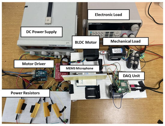
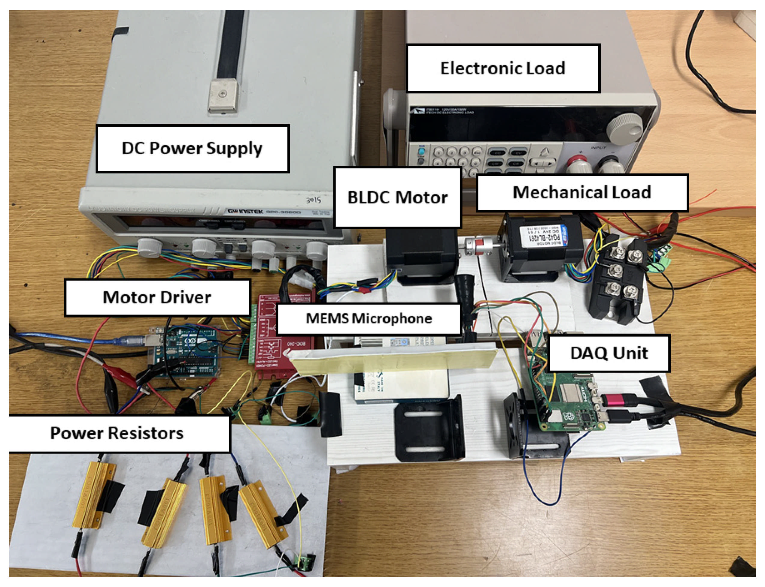
Figure 1 illustrates the experimental setup used for acoustic data acquisition. A BL4261 three-phase BLDC motor (Robotmart Co., Ltd., Seoul. Republic of Korea) was driven by a BDD-240 driver (supplied by MotorBank, Seoul, Republic of Korea) operating at 20 V. An Arduino PWM command of 100 (on a scale of 0–255) was applied to the VSP speed-control input of the BDD-240 driver and maintained constant throughout data acquisition. An identical BLDC motor, mechanically coupled to the target motor, was connected to an ITECH electronic load (ITECH Electronic Co., Ltd., Nanjing, China) through a three-phase rectifier. The electronic load was operated in constant-current mode at 0.1 A.
Figure 1.
Experimental setup for acoustic signal acquisition from the BLDC motor. DC: direct current; BLDC: brushless direct current; MEMS: microelectromechanical systems; DAQ: data acquisition.
Acoustic signals were acquired at a sampling frequency of 48 kHz using an INMP441 MEMS microphone (InvenSense, San Jose, CA, USA) positioned 4 cm from the side of the target motor and connected to a Raspberry Pi 5 (Raspberry Pi Ltd., Cambridge, UK). The Raspberry Pi 5 was configured as a wireless access point, allowing recording initiation and file storage to be controlled remotely from a tablet through a custom web-based interface. The microphone position and orientation, load condition, and recording procedure were kept identical across all HRC severity conditions to maintain consistent measurement conditions. The six measurement sessions (D01–D06) were conducted on different days rather than obtained by dividing a single continuous recording session. During each session, 40 WAV files were acquired for each of the three HRC severity levels (0.5, 1, and 2 Ω), resulting in 120 files per session. Each WAV file was recorded in a separate 15-s recording operation rather than extracted from a longer continuous recording. The first 1 s of each recording was discarded, and the remaining 14 s were divided into 1-s segments for FFT-CNN feature extraction. The same experimental setup and nominal operating and acoustic acquisition settings were maintained across all sessions. However, session-specific environmental differences between recording days were not quantified.
2.2. High-Resistance Connection Fault Configuration
A high-resistance connection (HRC) fault occurs when deterioration of the contact condition at an electrical connection between the motor and drive circuit increases the connection resistance above its normal level. Increased connection resistance can produce an additional voltage drop in the affected phase, potentially altering the magnitude and balance of the phase currents. These electrical changes can affect the motor’s electromagnetic operating state, leading to variations in torque fluctuations and mechanical vibrations that may be reflected in the acoustic signals generated by the motor. Accordingly, this study investigates HRC severity classification using acoustic features associated with variations in connection resistance.
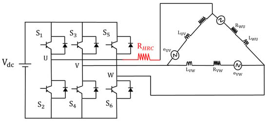
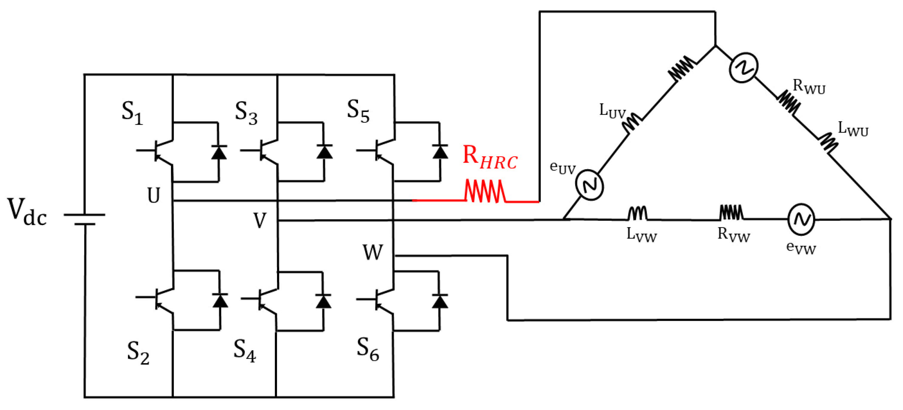
To emulate increased connection resistance, an external resistor was connected in series with the U-phase electrical connection of the BLDC motor. Three HRC severity levels were established based on the inserted resistance values: 0.5, 1, and 2 Ω. Throughout the experiments, the HRC was consistently introduced in the U phase, while the motor operating and acoustic measurement conditions were kept identical. Only the inserted resistance was varied to enable comparisons of acoustic characteristics across different connection-resistance levels. Figure 2 illustrates the HRC configuration used in this study.
Figure 2.
Schematic of the U-phase high-resistance connection fault configuration in the BLDC motor drive system.
3. Method
3.1. Problem Definition and Proposed Method
This study addresses the diagnosis of high-resistance connection (HRC) fault severity in BLDC motors using acoustic signals. HRC severity is represented by three resistance levels (0.5, 1, and 2 Ω), established by connecting an external resistor in series with the U-phase electrical connection of the motor. The objective is to classify the acquired acoustic signals into one of these three severity levels. Accordingly, this study focuses on classifying predefined HRC severity levels rather than detecting HRC faults relative to healthy operating conditions. An important consideration is intersession variation. Even signals acquired under the same HRC severity condition can exhibit different feature distributions because of variations in measurement time and experimental conditions. Consequently, distribution mismatches can arise between the class-specific feature distributions learned from the training sessions and those observed in a new, unseen session, potentially degrading HRC severity classification performance. Furthermore, session-dependent feature shifts are not necessarily consistent in magnitude or direction across different HRC severity classes. A feature extraction model is trained using a subset of the measurement sessions, while one session excluded from training is designated as the target session. Hereafter, the sessions used for model training are referred to as source sessions, whereas the unseen measurement session is referred to as the target session. During target-session evaluation, the trained feature extractor remains fixed, and the actual HRC severity labels of the target session are not used for feature correction or correction-strength selection.
The objective is to improve the robustness of HRC severity classification in unseen measurement sessions by reducing the positional mismatch between target features and fixed source class prototypes caused by intersession variation. Rather than directly compensating for session-related differences in the raw acoustic signals, a feature representation suitable for discriminating HRC severity levels is first learned from the source sessions. The target feature positions are then adjusted within this learned feature space.
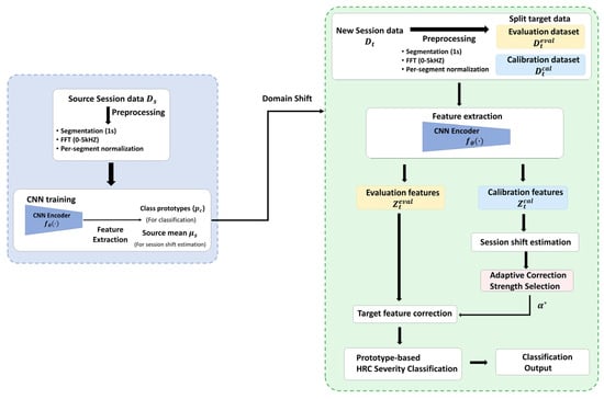
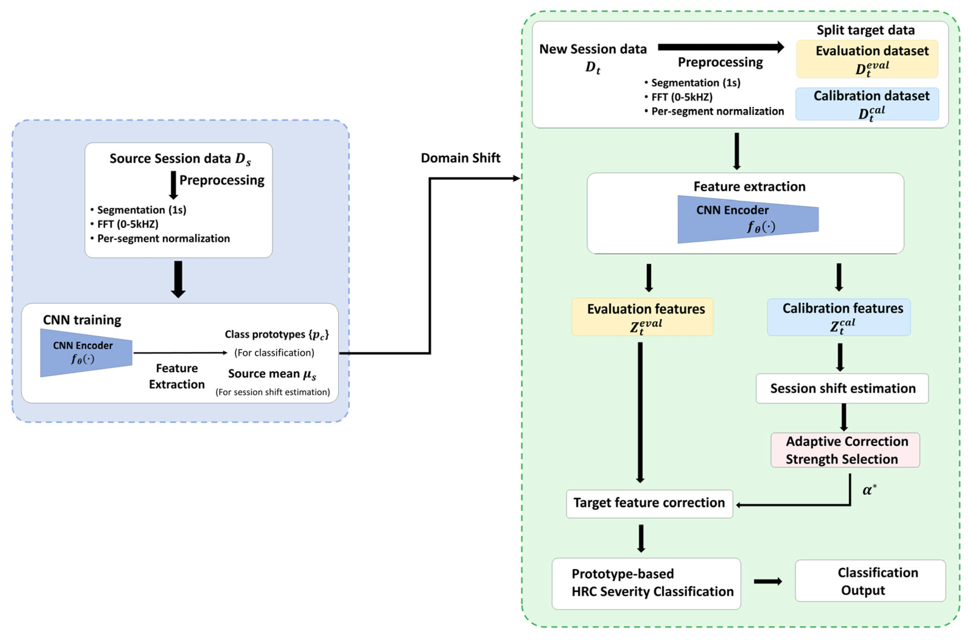
Figure 3 illustrates the proposed HRC severity classification procedure. First, a CNN encoder is trained using data from the source sessions, and the source class prototypes and global source mean feature vector are constructed from the extracted features. Data from a new target session are divided into separate calibration and evaluation sets, both of which undergo identical preprocessing and feature extraction using the fixed CNN encoder. The global mean-difference vector is estimated by subtracting the global source mean feature vector from the mean feature vector of the calibration set, and the correction strength is determined using ACSS. The evaluation features are then corrected by subtracting the estimated global mean-difference vector scaled by the selected . Finally, HRC severity is classified based on cosine similarity to the fixed source class prototypes. Thus, the proposed method adjusts only the target feature positions without additional model training or modification of the classification structure.
Figure 3.
Overall architecture of the proposed HRC severity classification method. CNN: convolutional neural network; FFT: fast Fourier transform; HRC: high-resistance connection.
3.2. Source Feature Learning Based on FFT-CNN
To extract discriminative features for HRC severity classification from source-session acoustic signals, an FFT-based frequency representation combined with a one-dimensional convolutional neural network (CNN) was used. The acoustic signals acquired at a sampling frequency of 48 kHz were divided into 1-s segments, and the log-magnitude spectrum of each segment was calculated and normalized as follows:
where is the 1-s acoustic signal, is the mean value of the corresponding segment, is the Hann window, and and are the mean and standard deviation of the log-magnitude spectrum of the corresponding segment, respectively. Normalization was performed independently for each 1-s segment. Only frequency components within the 0–5 kHz range were used as CNN inputs.
A CNN comprising three one-dimensional convolutional blocks was used to extract discriminative features from the FFT representation. Each block consisted of a one-dimensional convolutional layer, batch normalization, and ReLU activation. The detailed architecture is presented in Table 1. Following the final convolutional block, global average pooling was applied to obtain a 64-dimensional feature vector for each 1-s segment.
Table 1.
CNN architecture for FFT-based feature extraction.
During training, a linear classifier with three output nodes was connected to the 64-dimensional feature representation. The CNN feature extractor and linear classifier were jointly optimized by minimizing the cross-entropy loss using the source-session class labels. Through this training process, the CNN learned a 64-dimensional feature representation that discriminated among the HRC severity levels in the source sessions. Session-balanced mini-batches were constructed to ensure equal representation of each source session. For each leave-one-session-out (LOSO) fold, 12 signal segments were selected from each of the five source sessions, resulting in 60 segments per mini-batch. The model was trained for 15 epochs using the Adam optimizer with a learning rate of and a weight decay of . During subsequent target-session evaluation, the trained CNN feature extractor remained fixed.
3.3. File-Level Feature Construction and Cosine Prototype Classification
The CNN feature extractor trained as described in Section 3.2 generates a 64-dimensional feature vector for each 1-s acoustic signal segment. Because each original WAV file contains multiple 1-s segments, the corresponding segment-level feature vectors were averaged to obtain a single file-level feature vector. For an original WAV file consisting of segments, where denotes the feature vector extracted from the -th segment, the file-level feature is defined as:
Subsequent prototype construction and classification were performed using these file-level feature vectors. For each LOSO fold, a representative feature vector for each HRC severity class was constructed using the file-level features from the source sessions. Let denote the set of source files belonging to class . The class-mean feature vector was calculated as:
The resulting class-mean feature vector was L2-normalized to obtain the class prototype .
Thus, each class prototype is a unit vector satisfying . These source class prototypes remained fixed and served as reference vectors for classification during target-session evaluation. The feature vector of each target file was also L2-normalized before calculating cosine similarity:
For a target file , the classification score for class was defined as the cosine similarity between the normalized file-level feature vector and the corresponding class prototype:
Each target file was then assigned to the class with the highest classification score:
To evaluate the effect of target feature correction, BASE was defined as the baseline condition in which the uncorrected target file feature vector was directly classified using the cosine prototype classifier described above. The target feature correction procedure is described in the following section.
3.4. Target Feature Correction Based on Global Mean Difference
To mitigate positional mismatches between source- and target-session features, the target file-level feature vectors were corrected using a global mean-difference vector estimated from a subset of files in the target session. This vector represents the overall displacement of the target calibration features relative to the source features without estimating class-specific shifts or assuming that such shifts have identical directions and magnitudes across classes.
In each LOSO fold, 45 files were randomly selected from the 120 target-session files to form the calibration set (CAL45), while the remaining 75 files constituted the evaluation set (EVAL75). Each target session contained 40 files per HRC severity class. CAL45 was constructed without using class labels or enforcing a balanced class distribution. Let denote the mean of all file-level vectors from the source sessions, and let denote the mean of all file-level feature vectors in CAL45. The global mean difference vector for CAL45, , was defined as follows:
where represents the displacement from the global source mean to the global CAL45 mean and is calculated without using class-specific information.
For a target file , let denote its file-level feature vector before correction. The corrected feature vector is defined as:
where denotes the correction strength. The same correction vector is applied to all target file-level feature vectors rather than using separate correction vectors for individual classes. The correction strength, , is determined using ACSS, as described in Section 3.5.
Feature correction is performed in the 64-dimensional file-level feature space before L2 normalization. The corrected feature vectors are then subjected to the same L2 normalization and cosine prototype classification procedures described in Section 3.3. Thus, the classification criterion remains unchanged after feature correction, and the final HRC severity is determined by comparing the corrected target features with the fixed source class prototypes.
3.5. Adaptive Correction Strength Selection (ACSS)
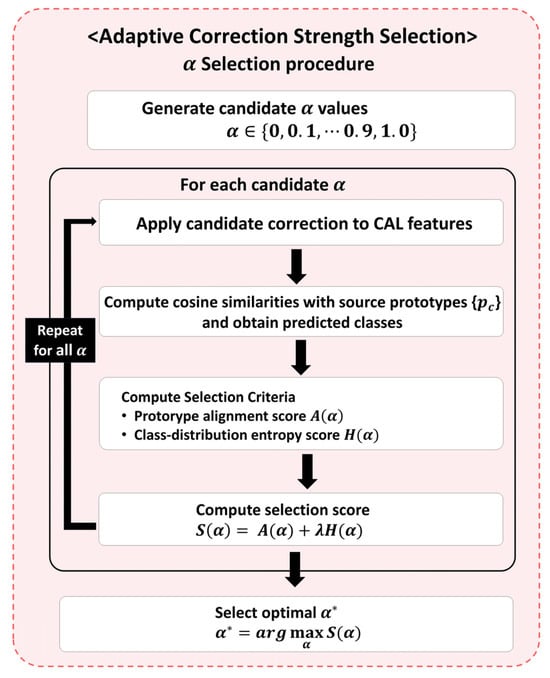
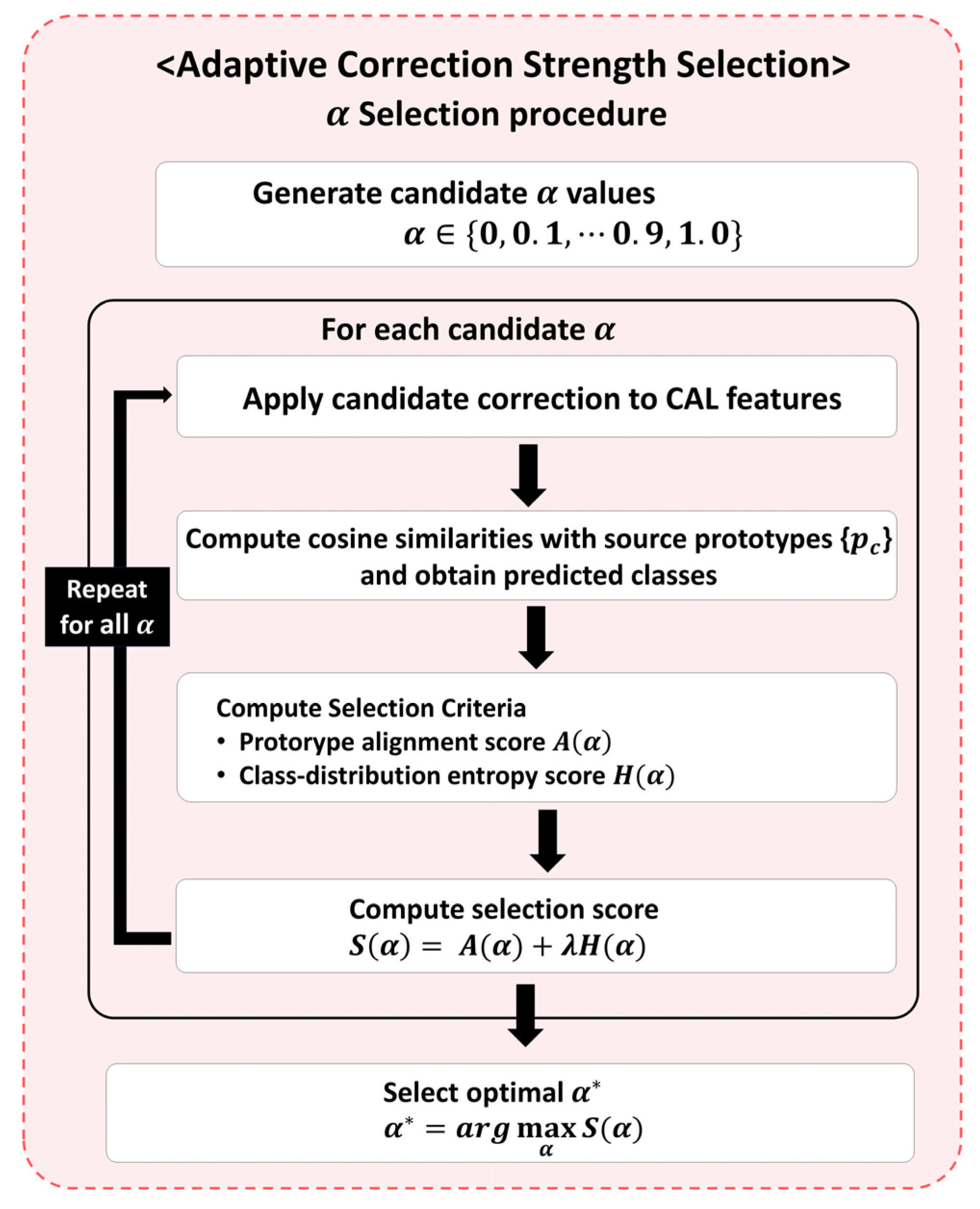
The appropriate degree of correction using the global mean-difference vector may vary across target sessions. Therefore, ACSS is proposed to automatically determine the correction strength without using the actual class labels of CAL45. In ACSS, candidate values of α range from 0 to 1 in increments of 0.1. Here, represents no feature correction, whereas represents full application of the global mean-difference vector estimated from CAL45, shifting the mean of the corrected CAL45 features to the global source mean. This candidate range allows the correction strength to be selected for each target session between these two extremes. For each candidate , the CAL45 features are corrected, and the resulting features are evaluated against the fixed source class prototypes. Two criteria are considered: prototype alignment and prediction-distribution entropy. The overall ACSS procedure, from generating candidate correction strengths to selecting the final , is illustrated in Figure 4.
Figure 4.
Procedure of the proposed Adaptive Correction Strength Selection (ACSS) using unlabeled CAL45 features. CAL: calibration.
As illustrated in Figure 4, the evaluation procedure is repeated for each candidate , and a selection score is calculated. To define the two criteria used in this score, let denote the feature vector of the i-th CAL45 file after correction using candidate . This feature vector is obtained by applying the correction defined in Section 3.4. The prototype alignment score is calculated as the average maximum cosine similarity between the corrected CAL45 feature vectors and the three source class prototypes:
A larger indicates higher average cosine similarity between the corrected CAL45 feature vectors and their most similar source class prototypes. However, selecting based solely on prototype alignment may favor candidates that produce an excessively concentrated prediction distribution, with most CAL45 files assigned to a single class. To discourage such concentration, prediction-distribution entropy is incorporated as a second criterion. Let denote the proportion of CAL45 files predicted to belong to class for candidate . The entropy is calculated as:
A larger indicates a more dispersed prediction distribution, with predictions distributed more broadly across classes rather than concentrated in a single class. This criterion is not intended to estimate the actual class composition or class proportions of CAL45. Instead, it discourages candidate corrections that produce excessive prediction concentration in a single class. Nevertheless, the global mean-difference vector may also reflect differences in class composition between the source data and CAL45, particularly when the calibration set exhibits substantial class imbalance. Furthermore, the entropy criterion may favor a more dispersed prediction distribution even when the calibration data contain predominantly or exclusively one severity class.
The final selection score is defined as the weighted sum of the prototype alignment score and prediction-distribution entropy:
where is a weighting factor that controls the relative contribution of the two criteria and was set to in this study. The final correction strength is selected as the candidate with the largest :
If two or more candidates yield the same maximum score, the smaller is selected. Finally, the selected is applied to EVAL75 using the feature correction defined in Section 3.4, and the corrected features are classified using the cosine prototype classification procedure described in Section 3.3.
3.6. Evaluation Protocol and Comparative Methods
3.6.1. Evaluation Protocol and Metrics
To evaluate generalization across measurement sessions, a leave-one-session-out (LOSO) evaluation protocol was adopted using six measurement sessions (D01–D06). In each fold, five sessions served as the source sessions for model training, while the remaining session was designated as the target session.
Following the CAL45/EVAL75 partition defined in Section 3.4, 20 random splits were generated for each target session to account for variability arising from calibration-set selection. Data partitioning was performed at the original WAV-file level to ensure that segments from the same WAV file were not shared between source-model training and target-session evaluation or between CAL45 and EVAL75 within each split.
The proposed method and the comparison methods were evaluated using five training seeds, with the same 20 splits applied across all methods and seeds. All methods used the same source-training strategy based on session-balanced mini-batches and the fixed source-prototype classification procedure. The rationale for selecting this training strategy, denoted as B1, is presented in Section 4.1. For the proposed method and the unlabeled comparison methods, calibration and adaptation were performed using only unlabeled CAL45 data, while EVAL75 was reserved for performance evaluation. For the label-informed class-conditional reference methods, the actual CAL45 labels were used to estimate class-specific correction vectors. In the grid oracle, EVAL75 labels were additionally used exclusively for retrospective correction-strength selection, as described in Section 3.6.2.
Classification performance was evaluated primarily using file-level Accuracy and Macro-F1. For each training seed, the evaluation results were first averaged across the 20 random splits for each target session and then across the six target sessions. Overall mean performance and seed-level standard deviations were calculated from the resulting five seed-level values. Where reported, 95% confidence intervals were calculated using the Student’s t-distribution based on these five values. For each target session, the 95% confidence interval of the Accuracy gain was calculated from the five paired seed-level differences between Proposed and BASE, with results first averaged across the 20 evaluation splits for each seed. Subsequent feature-space, class-wise, and classification-decision analyses were conducted using the LOSO evaluation results.
3.6.2. Comparative Adaptation Methods
To evaluate the proposed feature correction method against existing adaptation approaches, Correlation Alignment (CORAL) [43] and Test-Time Entropy Minimization (TENT) [44] were selected as representative methods of domain adaptation (DA) and test-time adaptation (TTA), respectively. CORAL reduces distribution mismatches by aligning feature statistics, whereas TENT adapts model parameters by minimizing prediction entropy. Both methods were evaluated using the protocol described in Section 3.6.1.
For CORAL, target-to-source alignment was adopted to preserve the source feature space and class prototypes. Let and denote the mean vectors of the source file-level features and unlabeled CAL45 features, respectively, and let and denote their corresponding covariance matrices. The Ledoit–Wolf shrinkage estimator [45] was used to estimate both covariance matrices. For a target file-level feature vector , the aligned feature was calculated as follows:
Unlike conventional covariance-only CORAL, the implemented transformation incorporated mean alignment in addition to covariance alignment. The transformation was applied before L2 normalization, while the trained CNN feature extractor and source class prototypes remained fixed. Classification was subsequently performed using the cosine prototype classifier described in Section 3.3.
For TENT, adaptation was restricted to the unlabeled CAL45 data, and this implementation was designated as TENT-CAL45. Only the affine parameters (γ and β) of the batch-normalization layers were updated, while the remaining CNN parameters and source class prototypes were kept fixed. Prediction probabilities were obtained by applying softmax to the cosine similarities between file-level features and source class prototypes, with the similarities scaled by a fixed factor of 10 to control the sharpness of the resulting probability distribution. For a calibration mini-batch B, the entropy-minimization objective was defined as follows:
where denotes a mini-batch of calibration files, is the number of files in the mini-batch, and is the predicted probability of class for file .
The 45 calibration files were randomly shuffled and divided into five mini-batches, each containing nine files. For each mini-batch, all 1-s segments from the nine WAV files were processed together, and the resulting segment-level features were averaged within each file to calculate the file-level prediction entropy. During adaptation, the model was operated in training mode, allowing the batch-normalization layers to use the statistics of the current mini-batch. The affine parameters were updated using stochastic gradient descent with a learning rate of 0.001, with one update step performed per mini-batch. Following the five update steps, the batch-normalization running statistics were reset and re-estimated using CAL45. These statistics were subsequently fixed during EVAL75 evaluation, with no further parameter updates. This CAL45-constrained implementation therefore differed from the original online TENT procedure.
For both comparison methods, adaptation was performed without using the actual target class labels, and the source class prototypes remained fixed. Accordingly, statistical feature alignment and normalization-based parameter adaptation were evaluated alongside the proposed feature correction method under identical calibration-data conditions.
To further investigate the limitations of global correction under heterogeneous class-wise feature shifts, two class-conditional correction methods were also evaluated. For each class c, the class-specific correction vector was defined as follows:
where and denote the calibration and source mean feature vectors for class c, respectively. The pseudo-label-based method (Pseudo-CC) estimated the calibration class means using BASE predictions, whereas the label-informed method (CAL-Label-CC) used the actual CAL45 class labels. For Pseudo-CC, the correction vector was set to zero if no calibration file was assigned to a particular class.
For both methods, the classification score for candidate class c was calculated by applying the corresponding class-specific correction vector to the target feature vector:
The predicted class was determined by selecting the candidate class with the highest classification score. The correction strength was fixed at = 1 for all classes in these comparisons. Neither method required the actual EVAL75 class labels, and the CNN feature extractor and source class prototypes remained fixed.
A class-conditional grid oracle was additionally evaluated to estimate the potential performance achievable within a predefined range of class-specific correction strengths. Using the class-specific correction vectors estimated from the actual CAL45 labels, was independently varied over {0, 0.25, 0.50, 0.75, 1.00} for each of the three classes. Among the resulting 125 combinations, the combination yielding the highest EVAL75 Accuracy was selected retrospectively. EVAL75 labels were used exclusively for this selection and not for assigning individual files to class-specific correction vectors. Accordingly, the grid oracle represents an optimistic reference within the defined correction framework rather than a deployable method or a universal theoretical upper bound.
4. Experimental Results and Analysis
This section evaluates the diagnostic performance of the proposed feature correction method under intersession variation. First, different source-training strategies are compared. The proposed method is then evaluated against BASE and representative adaptation methods. Finally, the characteristics of the learned feature space and the effects of feature correction on classification decisions are examined.
4.1. Source Training Strategy Comparison
To examine how mini-batch construction during source training affects generalization to unseen target sessions, four training strategies (B0–B3) were compared. These strategies differed in whether session balancing was applied and whether multiple segments originating from the same WAV file were restricted within a mini-batch. In this comparison, the generalization performance of each source-training strategy was evaluated using BASE classification without target feature correction.
Session-balanced mini-batches were used to reduce training bias toward individual source sessions and encourage the learning of discriminative features that incorporate information from all source sessions more evenly. The performance of the four training strategies is summarized in Table 2.
Table 2.
Performance comparison of B0–B3 source-training strategies.
The mean Accuracy of B0, which used random mini-batches, was 86.94%. Applying session balancing in B1 increased Accuracy to 90.50%, representing an improvement of 3.56 percentage points (pp). In addition, the standard deviation of Accuracy across training seeds decreased from 4.16% to 2.01%, indicating reduced variability associated with model initialization.
In contrast, B2 and B3, which restricted the inclusion of multiple segments from the same WAV file within a mini-batch, achieved Accuracies of 87.47% and 89.56%, respectively. Neither strategy outperformed B1. Macro-F1 was also highest for B1, at 0.8962, among the four strategies.
Based on these results, B1, which incorporated session-balanced mini-batches without restricting multiple segments from the same WAV file within a mini-batch, was selected as the source-training strategy for the subsequent experiments. Accordingly, all subsequent comparisons involving BASE, the proposed method, and the existing adaptation methods, as well as the feature-space analyses, were conducted using B1. However, because B1 was selected based on BASE performance across the same LOSO target sessions used in the subsequent evaluations, the training-strategy selection and final performance evaluation were not fully independent.
4.2. Overall Performance of the Proposed Feature Correction Method
Based on the comparison presented in Section 4.1, B1, which uses session-balanced mini-batches, was adopted as the source-training strategy for the subsequent experiments. To evaluate the effectiveness of the proposed feature correction method, its diagnostic performance was compared with that of BASE and the representative DA and TTA methods described in Section 3.6.2. The overall results are summarized in Table 3.
Table 3.
Overall diagnostic performance comparison.
As shown in Table 3, the proposed method increased mean Accuracy from 90.50% for BASE to 97.51%, corresponding to an improvement of 7.01 percentage points (pp). Macro-F1 also increased from 0.8962 to 0.9747, indicating improved classification performance across the three HRC severity classes. In addition, the standard deviation of Accuracy across training seeds decreased from 2.01% to 0.81%, indicating lower variability across training seeds than that observed for BASE.
Among the existing adaptation methods, CORAL achieved an Accuracy of 95.12% and a Macro-F1 of 0.9507, representing substantial improvements over BASE. The proposed method achieved a 2.39 pp higher Accuracy and a higher Macro-F1 than CORAL, although CORAL exhibited a lower seed standard deviation of 0.59%. CORAL aligned both the means and covariances of the target and source features, whereas the proposed method adjusted only the global mean difference using an adaptively selected correction strength. These results indicate that the proposed feature correction method achieved higher diagnostic performance than CORAL without requiring covariance alignment.
In contrast, TENT-CAL45 achieved an Accuracy of 68.20% and a Macro-F1 of 0.6088, indicating a substantial reduction in performance relative to BASE. To investigate the cause of this degradation, an additional diagnostic analysis was conducted using the models trained with seed 42. Re-estimating the batch-normalization statistics using CAL45 without updating the affine parameters produced the same Accuracy as TENT-CAL45 across all 20 splits for each target session. Furthermore, the two configurations produced identical file-level predictions for all 450 evaluation files examined in split 0 across the six target sessions (75 files per session). In contrast, applying the adapted affine parameters while retaining the original source batch-normalization statistics preserved the BASE Accuracy in the same split-0 evaluation.
These findings suggest that the performance degradation was primarily associated with the re-estimation of batch-normalization statistics rather than the entropy-based parameter updates. Because the source class prototypes were constructed using features extracted under the original source batch-normalization statistics, re-estimating these statistics using CAL45 could alter the positions of target features relative to the fixed prototypes. This change may explain the observed reduction in diagnostic performance under the TENT-CAL45 configuration.
4.3. Ablation and Sensitivity Analyses
To distinguish the contributions of global mean correction and ACSS, an ablation analysis was conducted using three configurations: BASE without feature correction ( = 0), global mean correction with a fixed strength ( = 1), and the proposed method with ACSS. Additional sensitivity analyses examined the effects of the entropy weighting factor and the number of calibration files. All comparisons used the fixed source-trained feature extractors and class prototypes, without additional model training. For the calibration-size analysis, CAL15 and CAL30 were constructed as nested subsets of CAL45, while the same EVAL75 set was retained for performance evaluation. The results are summarized in Table 4.
Table 4.
Ablation and sensitivity analyses of global mean correction and ACSS.
Global mean correction with = 1 achieved an Accuracy of 96.24%, compared with 90.50% for BASE. Incorporating ACSS further increased Accuracy to 97.51%. These results indicate that global mean correction accounted for most of the improvement over BASE, while adaptive correction-strength selection provided an additional improvement over fixed full correction. When prototype alignment alone was used for ACSS ( = 0), Accuracy decreased to 92.69%. Incorporating prediction-distribution entropy ( = 1) increased Accuracy to 97.51%, indicating that the entropy criterion contributed to the effectiveness of correction-strength selection. A comparable Accuracy of 97.50% was obtained with = 0.5, indicating limited sensitivity to the choice of positive entropy weighting factor.
Regarding calibration size, Accuracy increased from 95.98% with CAL15 to 97.15% with CAL30 and 97.51% with CAL45. These results indicate that relatively high diagnostic performance was achieved even with 15 unlabeled calibration files, although using 45 files yielded the highest Accuracy among the evaluated calibration sizes.
4.4. Feature-Space Characteristics Under Session Variation
To characterize the feature space under session variation, the separation among source classes was first compared with the magnitude of within-class variation across source sessions. Source class separation was calculated as the Euclidean distance between each pair of class centroids. The mean and minimum pairwise distances were defined as the mean and minimum source class separation, respectively.
Within-class source-session variation was calculated for each LOSO fold by averaging, across classes and source sessions, the Euclidean distances between each source-session class centroid and the corresponding representative source class centroid calculated using data from all source sessions. This metric, referred to as within-class source-session dispersion, quantifies the variation in class-centroid positions across measurement sessions for the same HRC class. To compare the relative scales of class separation and session variation, the ratio of the mean source class separation to within-class source-session dispersion was also calculated.
To quantify target-session variation, the Euclidean distance between each target class centroid and its corresponding source class centroid was defined as the target shift. Two normalized measures were then calculated: the mean target shift divided by the mean source class separation and the maximum target shift divided by the minimum source class separation. The former compares the average target shift with the average source class separation, whereas the latter compares the largest target shift with the minimum source class separation. These metrics are summarized in Table 5.
Table 5.
Summary of feature-space geometry under session variation.
As shown in Table 5, the mean source class separation was approximately 6.5 times the within-class source-session dispersion. This indicates that, although class centroids varied across source sessions, the separation between HRC severity classes was substantially greater than the within-class variation across sessions. Meanwhile, the mean target shift was approximately 0.33 times the mean source class separation, whereas the maximum target shift was approximately 0.54 times the minimum source class separation. Thus, although feature-centroid positions changed across measurement sessions, the target shifts were generally smaller than the class separation in the source feature space. However, these relative magnitudes do not establish whether the class-wise centroid shifts occurred in similar directions. To examine this, the directions of the class-wise centroid shifts were compared for each target session.
Let and denote the source and target feature centroids of class c, respectively. The class-wise target shift vector was defined as:
To assess directional similarity among class-wise centroid shifts, cosine similarities were calculated for the three pairs of shift vectors. Across all LOSO results, the mean cosine similarities for the 0.5–1 Ω, 0.5–2 Ω, and 1–2 Ω pairs were −0.0262 ± 0.2552, 0.1342 ± 0.4728, and −0.0683 ± 0.4943, respectively. Although variability across folds was substantial, the mean cosine similarities were close to zero, indicating no consistent positive directional alignment among the class-wise centroid shifts. These results suggest that class-wise centroid shifts do not consistently follow a common direction across target sessions.
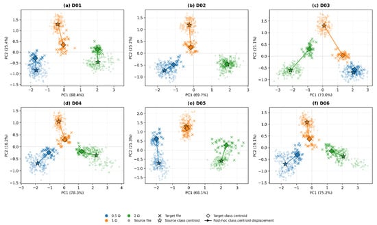
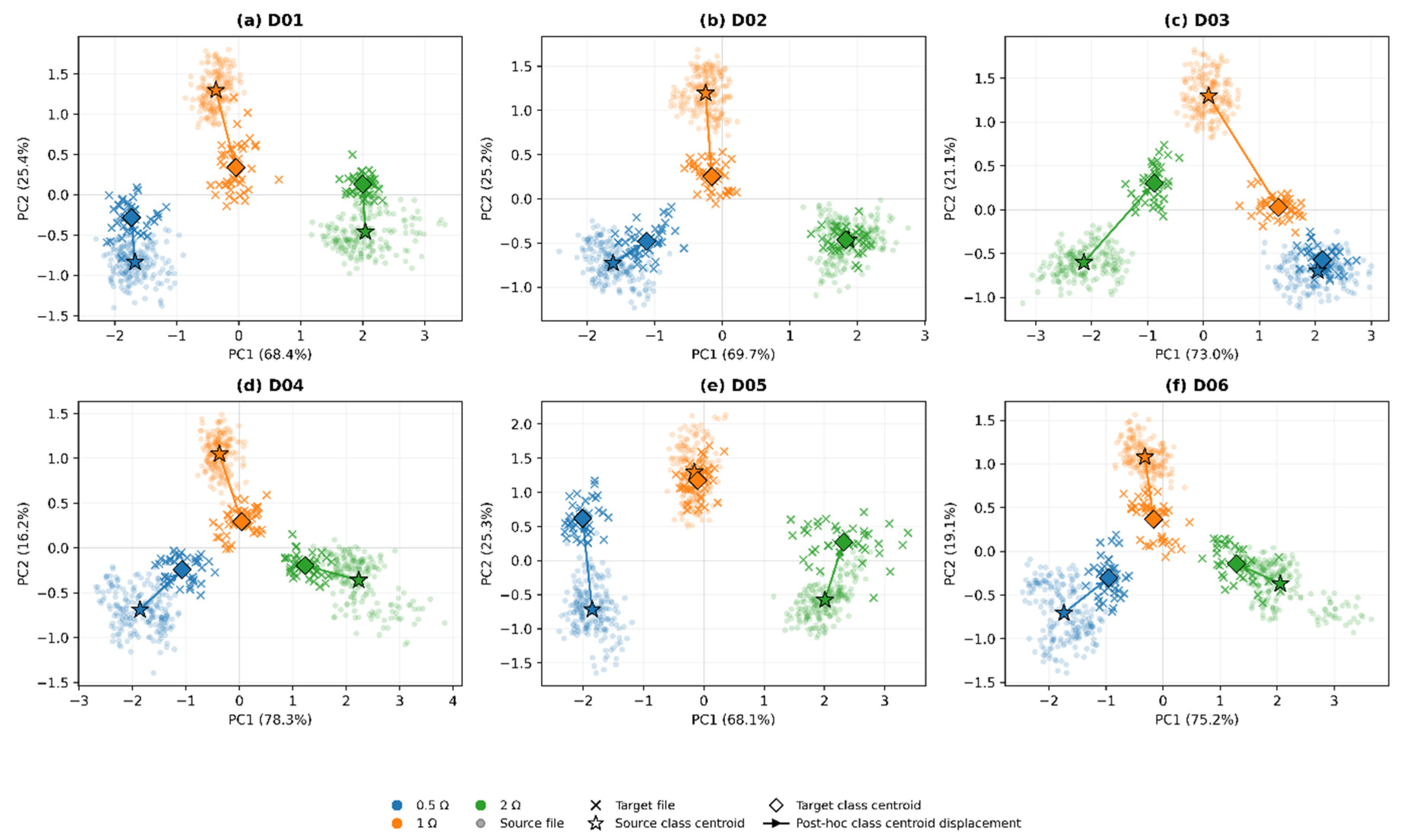
To visualize these feature-space characteristics, principal component analysis (PCA) axes were constructed using only the source file-level features in each LOSO fold. The source and target file-level features were then projected onto the same two-dimensional space. Figure 5 illustrates the class structures in each fold and the positional shifts of the target class centroids relative to their corresponding source centroids.
Figure 5.
PCA visualization of file-level CNN features for the six LOSO folds. (a) target session D01; (b) target session D02; (c) target session D03; (d) target session D04; (e) target session D05; (f) target session D06.
As shown in Figure 5, the target features retained distinct class-specific cluster structures, while the centroid of each target class shifted relative to its corresponding source centroid. The directions and magnitudes of these shifts varied across folds and classes, visually illustrating class-wise shift differences consistent with the quantitative analysis in the original 64-dimensional feature space. However, because PCA projects the 64-dimensional features onto two dimensions, the arrow lengths and angles in Figure 5 are used only for visualization and are not interpreted as quantitative measures of shift magnitude or direction in the original feature space.
4.5. Characteristics of Unlabeled Feature Correction
The extent to which the proposed method adjusted the learned feature space was analyzed. Across the overall LOSO evaluation, the mean selected correction strength, , was 0.6795, and the mean magnitude of the CAL45 global mean difference vector, , was 0.6452. Accordingly, the mean magnitude of the correction vector applied to the target features, , was 0.4459. To compare the applied correction with the scale of class separation in the source feature space, the correction-vector magnitude in each fold was normalized by the minimum source class separation. The normalized correction magnitude was, on average, 0.1757 times the minimum source class separation, corresponding to approximately 17.6%. This indicates that the proposed method applied a relatively limited positional adjustment compared with the existing class separation. In addition, a post hoc analysis examined the directional relationship between the CAL45-derived global mean-difference vector and the class-wise target shift vectors. The cosine similarities between these vectors for the 0.5, 1, and 2 Ω classes were 0.5455 ± 0.3153, 0.5723 ± 0.2049, and 0.4319 ± 0.3874, respectively. The class-wise target shifts were calculated from EVAL75 using ground-truth class labels solely for this post hoc analysis; these labels were not used for feature correction or ACSS. Although the mean cosine similarity was positive for all three classes, the variability across LOSO folds indicates that the degree of directional alignment varied. Thus, the global mean-difference vector does not provide an exact estimate of each class-wise shift. Rather, it captures a direction that is partially aligned, on average, with the class-wise shifts and can therefore be used for global feature correction.
To further assess the limitations of global correction under heterogeneous class-wise shifts, the proposed method was compared with the class-conditional correction methods described in Section 3.6.2. The results are summarized in Table 6.
Table 6.
Performance comparison of global and class-conditional feature correction methods.
As shown in Table 6, Pseudo-CC exhibited lower diagnostic performance than the proposed method, particularly in D03, whereas CAL-Label-CC and Grid Oracle achieved higher accuracy. These findings suggest that the effectiveness of class-conditional correction depends on the reliability of the class information used to estimate the correction vectors. The higher performance of the label-informed references also indicates that a single global correction vector does not fully capture the potential benefits of class-specific correction.
Nevertheless, the proposed method substantially outperformed Pseudo-CC without requiring target class labels or pseudo-label-based class assignments. By estimating a single global mean-difference vector from unlabeled calibration data, the proposed method mitigated session-dependent classification degradation despite heterogeneous class-wise shifts. This result highlights the practical value of the proposed approach when reliable class-specific information is unavailable.
4.6. Classification Decision Changes and Session-Wise Effects
This section examines how the proposed feature correction changes classification decisions relative to the fixed source prototypes. For this analysis, each EVAL75 result was assigned to one of four transition types according to whether it was correctly classified before and after correction. Cases that were correctly classified (C) both before and after correction were defined as C→C; cases that changed from misclassified (W) before correction to correctly classified after correction were defined as W→C; cases that changed from correctly classified to misclassified were defined as C→W; and cases that remained misclassified before and after correction were defined as W→W. The actual EVAL75 class labels were used only for the post hoc prediction-transition and classification-margin analyses.
The analysis included 45,000 repeated evaluation events obtained from six target sessions, five training seeds, 20 CAL45/EVAL75 splits per session, and 75 EVAL75 files per split. Because the same original WAV file could be evaluated repeatedly under different training seeds and CAL45/EVAL75 splits, these 45,000 events do not represent mutually independent physical files but rather repeated evaluation results.
To quantify the effect of correction on cosine-prototype classification decisions, the classification margin was calculated for each evaluation event. For a file-level feature with actual class , the classification margin was defined as the cosine similarity to the actual-class prototype minus the highest cosine similarity to an incorrect-class prototype.
A value of 0 indicates that the cosine similarity to the actual-class prototype exceeds the similarities to all other class prototypes, corresponding to a correct classification. Conversely, indicates that at least one other class prototype has a higher cosine similarity, corresponding to a misclassification. The prediction transitions and mean margin changes before and after correction are summarized in Table 7.
Table 7.
Prediction transitions and classification margin changes before and after feature correction.
Across all repeated evaluation events summarized in Table 7, 3243 events (7.21%) changed from W→C, whereas only 89 events (0.20%) changed from C→W. The difference between these transition rates, +7.01 pp, is consistent with the overall Accuracy improvement reported in Section 4.2 and shows how the overall performance gain arose from individual prediction transitions.
In particular, the mean margin of W→C events increased from −0.0174 before correction to 0.0202 after correction, representing an average transition from a negative to a positive margin. For W→W events, which remained misclassified after correction, the mean margin also increased from −0.0246 to −0.0084. Although these events did not cross the decision boundary, their margins shifted in a direction favorable to the actual class. In contrast, the mean margin change for C→C events was only +0.0001, indicating little change in the average margin of predictions that remained correct. C→W transitions accounted for only 0.20% of all evaluation events and had a mean pre-correction margin of 0.0034, indicating that these events were, on average, relatively close to the decision boundary before correction.
Overall, the proposed feature correction tended to improve the classification margins of previously misclassified events while largely preserving previously correct classifications. When the same correction vector is applied to all target features, the pairwise Euclidean distances between target features are preserved before L2 normalization. However, this common translation can alter the directions of target feature vectors relative to the fixed source class prototypes. Consequently, subsequent L2 normalization and cosine-similarity-based classification can produce different similarity scores and classification margins. We further analyzed how these prediction transitions and performance changes varied across target sessions. Table 8 presents the session-wise BASE and Proposed Accuracy values, the Accuracy gain with its 95% confidence interval, the W→C rate among BASE errors, and the ratio of mean target shift to mean source class separation defined in Section 4.4.
Table 8.
Session-wise BASE and proposed performance, Accuracy gain with 95% confidence interval, W→C transition rate, and relative feature shift.
Here, the W→C rate among BASE errors represents the proportion of evaluation events misclassified by BASE in each session that were correctly classified after correction. Its denominator therefore differs from that of the W→C rate in Table 7, which was calculated over all repeated evaluation events. This metric indicates the proportion of initial misclassifications recovered in each session.
As shown in Table 8, the effect of the proposed feature correction varied across target sessions, although Accuracy improved over BASE in five of the six sessions. In particular, D03 had the lowest BASE Accuracy, at 57.97%, which increased to 92.73% with the Proposed method, representing the largest improvement of +34.76 pp. D04 and D05 improved by +3.03 pp and +2.21 pp, respectively, while D01 and D06 improved by +1.09 pp and +1.00 pp, respectively. In contrast, D02 changed only from 99.20% to 99.16%, indicating virtually no difference in performance.
The median Accuracy gain across the six target sessions was 1.65 pp. Excluding D03, the mean Accuracy across the remaining five sessions was 97.00% for BASE and 98.46% for Proposed, corresponding to an improvement of 1.46 pp. These results indicate that the overall improvement of 7.01 pp was largely driven by D03, where the most severe BASE performance degradation was observed. The 95% confidence interval of the Accuracy gain excluded zero only for D03, whereas the intervals for the other five sessions included zero. This result is particularly relevant to the objective of the proposed method, which is to mitigate diagnostic performance degradation caused by session-dependent feature mismatch. Across the six LOSO target sessions, the standard deviation of the session-wise Accuracy gains was 13.64 pp, indicating substantial between-session variability.
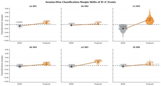
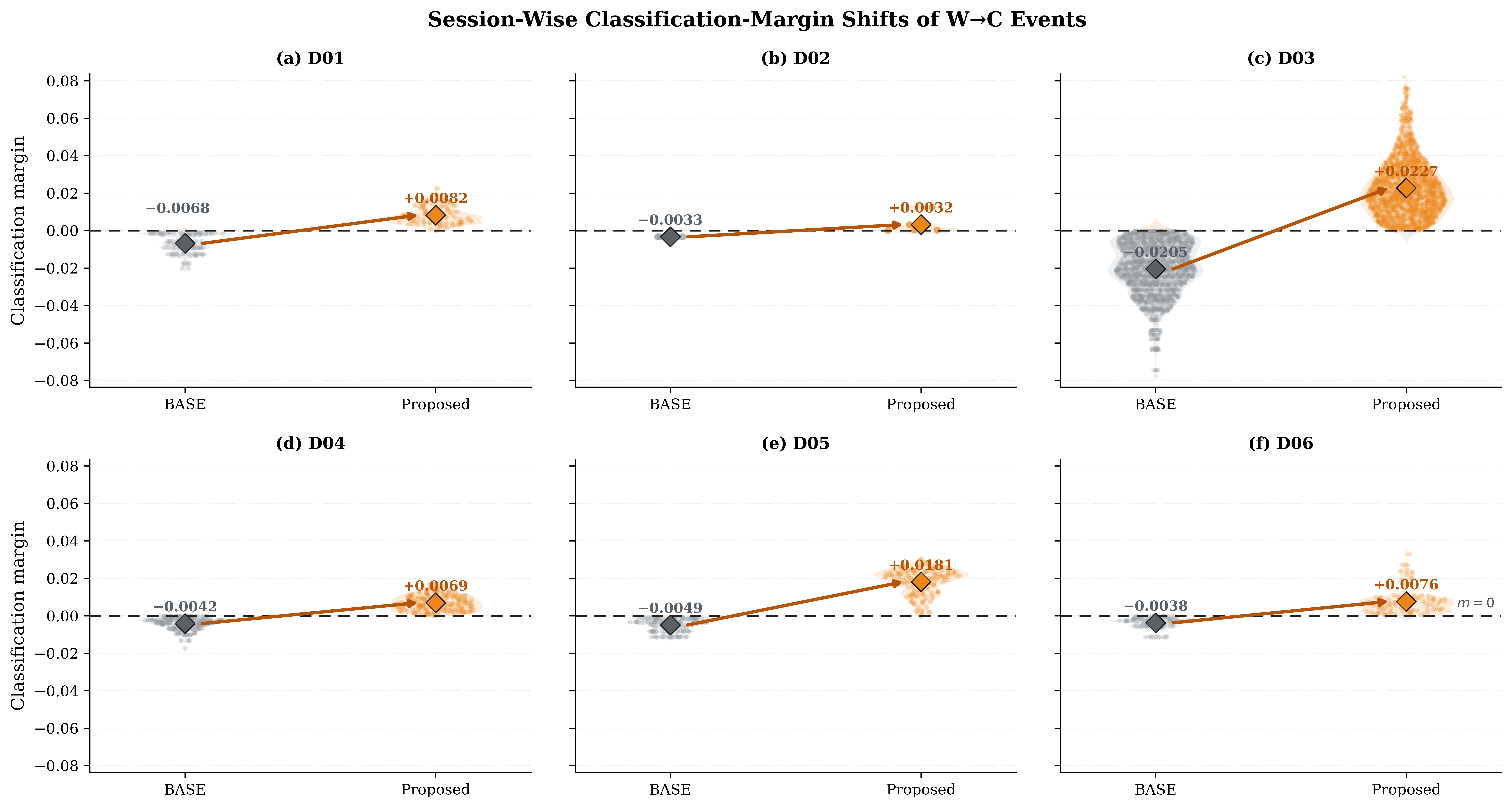
The W→C rate among BASE errors ranged from 8.33% to 92.22% across sessions. In D03, 82.71% of BASE errors were converted to correct classifications after correction. D05, despite its high BASE Accuracy of 97.60% and consequently small number of initial errors, also exhibited a high W→C rate of 92.22%. Thus, the magnitude of the session-wise Accuracy improvement depends not only on the proportion of BASE errors recovered through W→C transitions but also on the number of initial misclassifications and the occurrence of C→W transitions. To examine how W→C transitions were reflected in margin changes at the classification decision boundary, Figure 6 shows the distributions of classification margins before and after correction for repeated evaluation events that changed from W→C in each target session.
Figure 6.
Session-wise classification-margin shifts of W→C events: (a) targetsession D01; (b) target session D02; (c) target session D03; (d) target session D04; (e) target session D05; (f) target session D06.
As shown in Figure 6, W→C events in all sessions shifted from negative BASE margins to positive Proposed margins, crossing the decision boundary at zero. In particular, D03 exhibited the largest change, with the mean margin shifting from −0.0205 to +0.0227. This indicates that, after correction, the cosine similarity to the actual-class prototype exceeded that to the competing prototypes, resulting in the transition from misclassification to correct classification.
Meanwhile, the ratio of mean target shift to mean source class separation ranged from 0.248 to 0.405 across sessions, but no simple relationship was observed between this ratio and BASE performance. D05, which exhibited the largest relative shift (0.405), had a high BASE Accuracy of 97.60%, whereas D03, with a relative shift of 0.371, had the lowest BASE Accuracy of 57.97%. Therefore, session-wise classification performance cannot be explained solely by the magnitude of feature shifts; the relative positions of the shifted target features with respect to the source class prototypes also need to be considered.
4.7. Class-Wise Misclassification Structure and Repeated-Trial Consistency in D03
D03 exhibited the lowest BASE performance among the six target sessions and the largest performance improvement after the proposed correction. Therefore, the classes and prediction transitions contributing to the performance changes in D03 were further analyzed. The class-wise results are summarized in Table 9.
Table 9.
Class-wise BASE and proposed performance and W→C transition rates for D03.
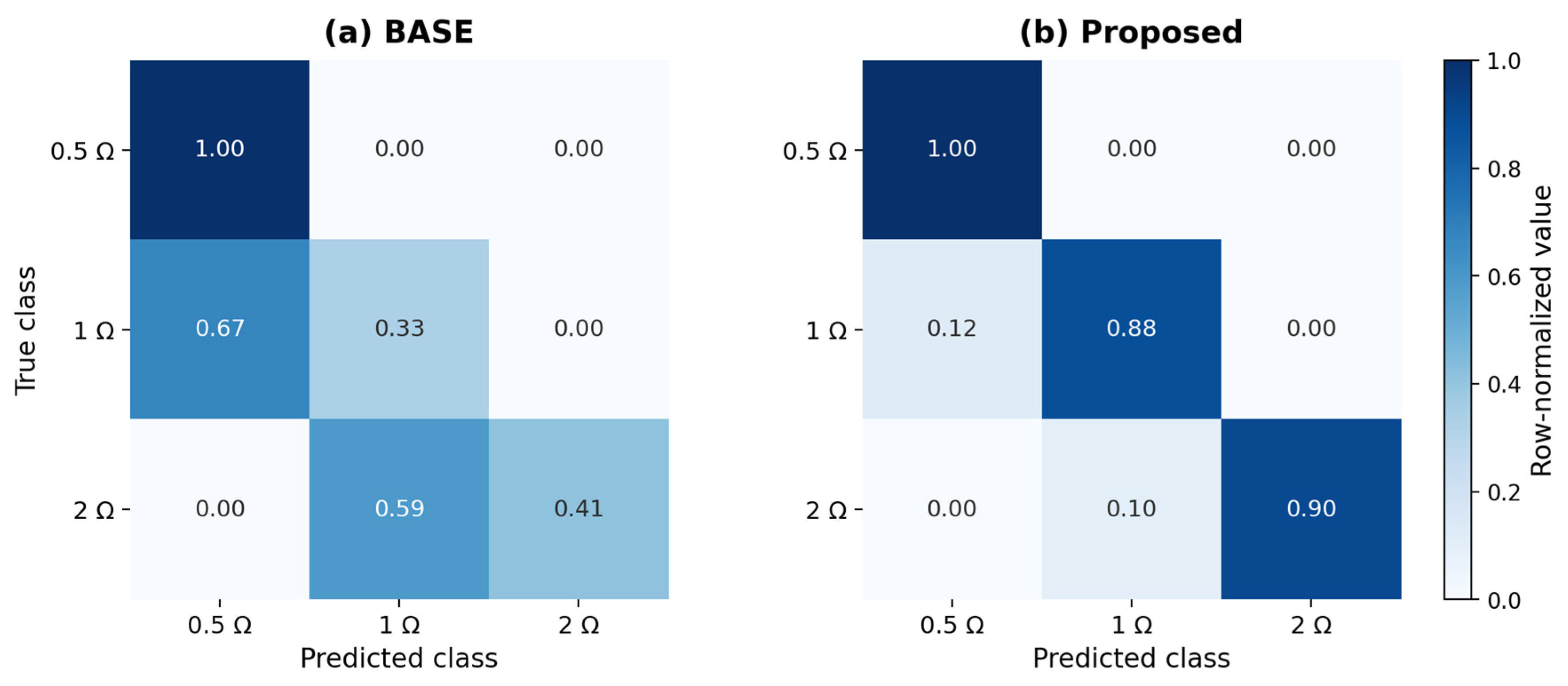
As shown in Table 9, performance degradation in D03 was not uniform across classes but was concentrated in the 1 Ω and 2 Ω classes. The 0.5 Ω class maintained 100% Accuracy under both BASE and Proposed, whereas the BASE Accuracy values for the 1 Ω and 2 Ω classes were 32.89% and 40.64%, respectively. These values increased to 87.91% and 90.22%, respectively, after correction. The W→C rates among BASE errors were also high, at 81.99% for 1 Ω and 83.52% for 2 Ω. These class-dependent outcomes are consistent with the decision mechanism discussed in Section 4.6, in which a common feature correction can change the relative cosine similarities of individual target features to the fixed source prototypes. Therefore, the observed recovery does not imply that the global correction vector accurately represents the underlying shift of each class.
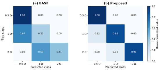
To examine the misclassification patterns associated with these class-wise performance changes, row-normalized confusion matrices were constructed from all repeated evaluation events in D03 for BASE and Proposed, as shown in Figure 7. Each row was normalized by the true class, and each cell represents the proportion of samples from the corresponding true class assigned to each predicted class.
Figure 7.
Row-normalized confusion matrices for D03 before and after feature correction: (a) BASE and (b) proposed.
As shown in Figure 7, BASE misclassifications were concentrated in specific class-to-class transitions rather than being distributed uniformly across classes. The 1 Ω class was misclassified primarily as 0.5 Ω, whereas the 2 Ω class was misclassified primarily as 1 Ω. Under Proposed, these off-diagonal proportions decreased substantially, while the diagonal proportions for the 1 Ω and 2 Ω classes increased. The 0.5 Ω class retained its 100% classification Accuracy. These results indicate that the performance degradation in D03 was associated with a structured class-confusion pattern toward adjacent lower resistance levels.
To further examine the recovery of these misclassifications, the W→C events were analyzed according to their BASE predictions. All 1370 W→C events for the 1 Ω class had been classified as 0.5 Ω under BASE, whereas all 1237 W→C events for the 2 Ω class had been classified as 1 Ω. Thus, the recovered errors followed the two dominant misclassification pathways identified above. In addition, the mean classification margin of W→C events increased from −0.0186 to 0.0205 for the 1 Ω class and from −0.0226 to 0.0251 for the 2 Ω class. Thus, for these events, the cosine similarity to an incorrect-class prototype exceeded that to the actual-class prototype before correction, whereas the actual-class prototype had the highest cosine similarity after correction.
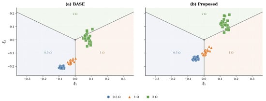
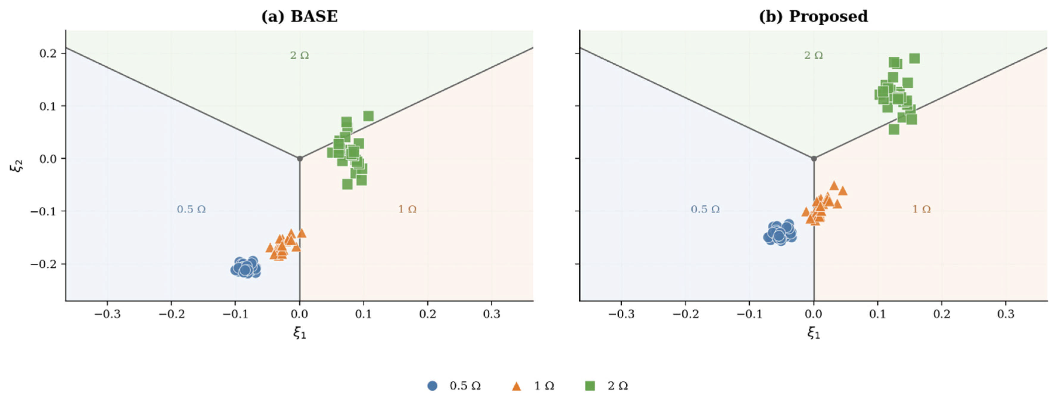
To examine how these class-wise misclassification transitions appeared in the decision structure of the cosine-prototype classifier, a single D03 evaluation condition (training seed 42, split 0) was selected as an example. The cosine scores before and after correction were transformed into a symmetric two-dimensional decision space, as shown in Figure 8. Let the cosine scores of an evaluation feature relative to the 0.5 Ω, 1 Ω, and 2 Ω prototypes be , , and , respectively. The visualization coordinates and were defined as follows:
Figure 8.
Class-wise changes in the symmetric cosine decision space of D03 for training seed 42 and split 0: (a) BASE and (b) proposed.
This transformation symmetrically arranges the relative cosine-score directions of the three classes at 120° intervals, while the three decision regions in the transformed space correspond exactly to the maximum-score prediction rule of the original cosine-prototype classifier.
As shown in Figure 8, the class-wise misclassification structure identified above was also evident in the decision space. Under BASE, many 1 Ω and 2 Ω features were positioned in decision regions associated with adjacent lower resistance levels, whereas under Proposed, a substantial proportion shifted into their corresponding correct-class decision regions. The classification structure of the 0.5 Ω features was maintained. Thus, the substantial performance improvement in D03 can be visualized as a spatial rearrangement associated with the correction of the dominant misclassification patterns.
Finally, to examine whether this recovery occurred only under specific training-seed or CAL45/EVAL75 split conditions, the consistency of repeated evaluations of the same original WAV files was analyzed. For the 75 distinct WAV files in D03 that had at least one BASE misclassification across repeated evaluations, the proportion of BASE-misclassified events converted to correct classifications after correction was calculated for each file.
The mean file-wise W→C transition rate was 86.74%, with a median of 97.14%. These results indicate that the recovery of correct classifications was observed repeatedly for the same WAV files across the evaluated training-seed and CAL45/EVAL75 split conditions. However, because the same physical WAV files were evaluated repeatedly under different training and split conditions, these repeated evaluation events were not treated as mutually independent experimental samples.
Overall, the low BASE performance of D03 was primarily associated with structured misclassifications in which the 1 Ω and 2 Ω classes were predicted as the adjacent lower resistance levels. The proposed feature correction altered the relative cosine relationships of these events in a direction favorable to the actual class, moving a substantial proportion into the correct decision regions. This transition pattern was also observed relatively consistently across repeated evaluations of the same original WAV files. However, the specific measurement or environmental factors responsible for the distinctive feature distribution in D03 could not be identified from the available data.
5. Conclusions
In this study, a feature-level correction method was proposed to mitigate session-dependent performance degradation in acoustic HRC severity diagnosis of BLDC motors. The method estimates a global mean-difference vector from source features and unlabeled target calibration data and automatically selects the correction strength using ACSS, while keeping the trained CNN feature extractor and source class prototypes fixed. In the LOSO evaluation across six measurement sessions, the proposed method increased mean Accuracy from 90.50% to 97.51%, an improvement of 7.01 pp, while Macro-F1 increased from 0.8962 to 0.9747. The standard deviation of Accuracy across training seeds also decreased from 2.01% to 0.81%, indicating lower variability across training seeds. In particular, for D03, which exhibited the lowest BASE performance, Accuracy increased from 57.97% to 92.73%, an improvement of 34.76 pp. The feature-space analyses showed that class-wise centroid shifts did not consistently follow a common direction across target sessions. The ratio of the applied correction magnitude to the minimum source class separation was approximately 17.6%. Nevertheless, the correction converted a substantial proportion of existing misclassifications into correct classifications and improved the classification margins of previously misclassified events. These findings suggest that a common feature-level correction can improve classification relative to fixed source class prototypes without explicitly estimating individual class-wise session shifts. However, a single global correction vector cannot fully account for heterogeneous class-wise shifts, which may limit its effectiveness when class-specific displacement patterns differ substantially.
This evaluation was limited to one BLDC motor, a fixed electronic-load setting and microphone position, and three U-phase HRC severity levels without a healthy class. Although the PWM control command was held constant, actual motor speed and shaft torque were not measured. Therefore, the contribution of possible resistance-induced changes in motor speed to the observed acoustic features could not be isolated. Additional controlled evaluations showed that diagnostic performance varied substantially with target-class composition. Accordingly, the reported 97.51% Accuracy under the original evaluation protocol should not be interpreted as evidence of robustness under severely imbalanced or single-class target conditions. Generalization to HRC faults in the V and W phases or at multiple connections, other motor units, different microphone positions, and varying operating and environmental conditions remains to be evaluated. The ability to distinguish healthy operation from HRC faults also remains untested. Future work will address these limitations and investigate the stability of ACSS with respect to calibration data, as well as its extension to other feature spaces and classification structures.
Author Contributions
Conceptualization, S.M.Y. and I.S.L.; methodology, S.M.Y. and I.S.L.; investigation, S.M.Y., and H.G.L.; experiments, S.M.Y., and H.G.L.; simulations, S.M.Y.; data analysis, S.M.Y. and I.S.L.; writing—original draft, S.M.Y.; writing—review and editing, S.M.Y. and I.S.L.; supervision, I.S.L. All authors have read and agreed to the published version of the manuscript.
Funding
This research received no external funding.
Institutional Review Board Statement
Not applicable.
Informed Consent Statement
Not applicable.
Data Availability Statement
The data are not publicly available due to ongoing research but are available from the corresponding author upon reasonable request.
Conflicts of Interest
The authors declare no conflicts of interest.
References
- Mohanraj, D.; Aruldavid, R.; Verma, R.; Sathiyasekar, K.; Barnawi, A.B.; Chokkalingam, B.; Mihet-Popa, L. A Review of BLDC Motor: State of Art, Advanced Control Techniques, and Applications. IEEE Access 2022, 10, 54833–54869. [Google Scholar] [CrossRef] [Scilit]
- Singh, B.; Singh, S. State-of-Art on Permanent Magnet Brushless DC Motor Drives. J. Power Electron. 2009, 9, 1–17. [Google Scholar] [CrossRef] [Scilit]
- Moseler, O.; Isermann, R. Application of Model-Based Fault Detection to a Brushless DC Motor. IEEE Trans. Ind. Electron. 2000, 47, 1015–1020. [Google Scholar] [CrossRef]
- Hou, Q.; Wang, H.; Zhao, C.; Xu, S.; Zuo, Y.; Lee, C.H.T.; Ding, S. Super-Twisting Extended State Observer-Based Quasi-Proportional-Resonant Controller for Permanent Magnet Synchronous Motor Drive System. IEEE Trans. Transp. Electrif. 2024, 10, 1596–1604. [Google Scholar] [CrossRef] [Scilit]
- Hou, Q.; Wang, H.; Lee, C.H.T.; Ding, S. Composite Adaptive Super-Twisting Sliding Mode Control Using Barrier Function for PM Motor Drives Toward Electric Aircraft Applications. IEEE Trans. Power Electron. 2025, 40, 16255–16264. [Google Scholar] [CrossRef] [Scilit]
- Tao, R.; Wang, W.; Luo, C.; Sun, L.; Cheng, M. Full-Torque Copper-Loss Minimum Adaptive Fault-Tolerant Control of Dual Three-Phase PMSM Under Open-Phase Faults. IEEE Trans. Transp. Electrif. 2026, 12, 1761–1774. [Google Scholar] [CrossRef] [Scilit]
- Tao, R.; Wang, W.; Jiang, Y.; Tang, C.; Fan, Y.; Hua, W. Free-Current-Curve Fault-Tolerant Control of Dual Three-Phase Permanent Magnet Synchronous Motor Under Open-Phase Fault. IEEE Trans. Transp. Electrif. 2025, 11, 11619–11631. [Google Scholar] [CrossRef] [Scilit]
- Shifat, T.A.; Hur, J.W. An Effective Stator Fault Diagnosis Framework of BLDC Motor Based on Vibration and Current Signals. IEEE Access 2020, 8, 106968–106981. [Google Scholar] [CrossRef] [Scilit]
- Da, Y.; Shi, X.; Krishnamurthy, M. Health Monitoring, Fault Diagnosis and Failure Prognosis Techniques for Brushless Permanent Magnet Machines. In Proceedings of the 2011 IEEE Vehicle Power and Propulsion Conference (VPPC), Chicago, IL, USA, 6–9 September 2011; pp. 1–7. [Google Scholar] [CrossRef] [Scilit]
- Kudelina, K.; Asad, B.; Vaimann, T.; Rassõlkin, A.; Kallaste, A.; Lukichev, D.V. Main Faults and Diagnostic Possibilities of BLDC Motors. In Proceedings of the 2020 27th International Workshop on Electric Drives: MPEI Department of Electric Drives 90th Anniversary (IWED), Moscow, Russia, 27–30 January 2020; pp. 1–6. [Google Scholar] [CrossRef] [Scilit]
- Luo, C.; Wang, J.; Miao, Q. Transient Current Ratio Dendrite Net for High-Resistance Connection Diagnosis in BLDCM. IEEE Trans. Power Electron. 2024, 39, 4746–4757. [Google Scholar] [CrossRef] [Scilit]
- Gupta, A.; Reddy, R.S.; Jayaraman, K. An Input Current-Based Method for Fault Diagnosis of High Resistance Connection in BLDC Motors. IEEE Sens. J. 2024, 24, 14844–14854. [Google Scholar] [CrossRef] [Scilit]
- Wang, H.; Lu, S.; Qian, G.; Ding, J.; Liu, Y.; Wang, Q. A Two-Step Strategy for Online Fault Detection of High-Resistance Connection in BLDC Motor. IEEE Trans. Power Electron. 2020, 35, 3043–3053. [Google Scholar] [CrossRef] [Scilit]
- Hadziefendic, N.; Trifunovic, J.; Kostic, M. Effects of a Reduced Torque on Heating of Electrical Contacts in Plugs and Receptacles. IEEE Trans. Compon. Packag. Manuf. Technol. 2018, 8, 1905–1913. [Google Scholar] [CrossRef] [Scilit]
- Yun, J.; Cho, J.; Lee, S.B.; Yoo, J.-Y. Online Detection of High-Resistance Connections in the Incoming Electrical Circuit for Induction Motors. IEEE Trans. Ind. Appl. 2009, 45, 694–702. [Google Scholar] [CrossRef] [Scilit]
- Hang, J.; Wu, H.; Ding, S.; Hua, W.; Wang, Q. A DC-Flux-Injection Method for Fault Diagnosis of High-Resistance Connection in Direct-Torque-Controlled PMSM Drive System. IEEE Trans. Power Electron. 2020, 35, 3029–3042. [Google Scholar] [CrossRef] [Scilit]
- Gangsar, P.; Tiwari, R. Signal Based Condition Monitoring Techniques for Fault Detection and Diagnosis of Induction Motors: A State-of-the-Art Review. Mech. Syst. Signal Process. 2020, 144, 106908. [Google Scholar] [CrossRef] [Scilit]
- Picazo-Ródenas, M.J.; Antonino-Daviu, J.; Climente-Alarcon, V.; Royo-Pastor, R.; Mota-Villar, A. Combination of Noninvasive Approaches for General Assessment of Induction Motors. IEEE Trans. Ind. Appl. 2015, 51, 2172–2180. [Google Scholar] [CrossRef] [Scilit]
- Huang, W.; Du, B.; Li, T.; Cheng, Y.; Cui, S. Detection of PMSM Demagnetization Fault and Eccentricity Fault Based on Acoustic Images and DeiT Classifier. IEEE Trans. Energy Convers. 2025, 40, 1870–1884. [Google Scholar] [CrossRef] [Scilit]
- Glowacz, A. Acoustic Based Fault Diagnosis of Three-Phase Induction Motor. Appl. Acoust. 2018, 137, 82–89. [Google Scholar] [CrossRef] [Scilit]
- Ma, L.; Zhang, Y.; Wang, Z. Fault Diagnosis of Motor Bearing Transmission System Based on Acoustic Characteristics. Sensors 2026, 26, 259. [Google Scholar] [CrossRef] [Scilit]
- Yao, Y.; Wang, H.; Li, S.; Liu, Z.; Gui, G.; Dan, Y.; Hu, J. End-To-End Convolutional Neural Network Model for Gear Fault Diagnosis Based on Sound Signals. Appl. Sci. 2018, 8, 1584. [Google Scholar] [CrossRef] [Scilit]
- Kiranyaz, S.; Devecioglu, O.C.; Alhams, A.; Sassi, S.; Ince, T.; Avci, O.; Gabbouj, M. Exploring Sound Versus Vibration for Robust Fault Detection on Rotating Machinery. IEEE Sens. J. 2024, 24, 23255–23264. [Google Scholar] [CrossRef] [Scilit]
- Uzel, H.; Özüpak, Y.; Alpsalaz, F.; Aslan, E.; Zaitsev, I. Acoustic-Based Fault Diagnosis of Electric Motors Using Mel Spectrograms and Convolutional Neural Networks. Sci. Rep. 2026, 16, 3379. [Google Scholar] [CrossRef] [Scilit]
- Luo, Y.; Lu, W.; Kang, S.; Tian, X.; Kang, X.; Sun, F. Enhanced Feature Extraction Network Based on Acoustic Signal Feature Learning for Bearing Fault Diagnosis. Sensors 2023, 23, 8703. [Google Scholar] [CrossRef] [Scilit]
- Chen, X.; Yang, R.; Xue, Y.; Huang, M.; Ferrero, R.; Wang, Z. Deep Transfer Learning for Bearing Fault Diagnosis: A Systematic Review Since 2016. IEEE Trans. Instrum. Meas. 2023, 72, 3508221. [Google Scholar] [CrossRef] [Scilit]
- Xiao, D.; Huang, Y.; Zhao, L.; Qin, C.; Shi, H.; Liu, C. Domain Adaptive Motor Fault Diagnosis Using Deep Transfer Learning. IEEE Access 2019, 7, 80937–80949. [Google Scholar] [CrossRef] [Scilit]
- Ahvazi, P.S.; Mohammadi, H. A High-Precision Voiceprint Recognition for Fault Diagnosis of Motor Bearings through Lightweight Dynamic Convolutional Neural Network. Results Eng. 2026, 29, 108463. [Google Scholar] [CrossRef] [Scilit]
- Li, X.; Zhang, W.; Ding, Q.; Sun, J.-Q. Multi-Layer Domain Adaptation Method for Rolling Bearing Fault Diagnosis. Signal Process. 2019, 157, 180–197. [Google Scholar] [CrossRef] [Scilit]
- Shen, C.; Wang, X.; Wang, D.; Li, Y.; Zhu, J.; Gong, M. Dynamic Joint Distribution Alignment Network for Bearing Fault Diagnosis under Variable Working Conditions. IEEE Trans. Instrum. Meas. 2021, 70, 3510813. [Google Scholar] [CrossRef] [Scilit]
- Qian, Q.; Zhou, J.; Qin, Y. Relationship Transfer Domain Generalization Network for Rotating Machinery Fault Diagnosis under Different Working Conditions. IEEE Trans. Ind. Inform. 2023, 19, 9898–9908. [Google Scholar] [CrossRef] [Scilit]
- Li, J.; Shen, C.; Kong, L.; Wang, D.; Xia, M.; Zhu, Z. A New Adversarial Domain Generalization Network Based on Class Boundary Feature Detection for Bearing Fault Diagnosis. IEEE Trans. Instrum. Meas. 2022, 71, 2506909. [Google Scholar] [CrossRef] [Scilit]
- Chen, L.; Li, Q.; Shen, C.; Zhu, J.; Wang, D.; Xia, M. Adversarial Domain-Invariant Generalization: A Generic Domain-Regressive Framework for Bearing Fault Diagnosis under Unseen Conditions. IEEE Trans. Ind. Inform. 2022, 18, 1790–1800. [Google Scholar] [CrossRef] [Scilit]
- Chai, Z.; Zhao, C. A Fine-Grained Adversarial Network Method for Cross-Domain Industrial Fault Diagnosis. IEEE Trans. Autom. Sci. Eng. 2020, 17, 1432–1442. [Google Scholar] [CrossRef] [Scilit]
- Zhang, Q.; Zhao, Z.; Zhang, X.; Liu, Y.; Sun, C.; Li, M.; Wang, S.; Chen, X. Conditional Adversarial Domain Generalization with a Single Discriminator for Bearing Fault Diagnosis. IEEE Trans. Instrum. Meas. 2021, 70, 3514515. [Google Scholar] [CrossRef] [Scilit]
- Chen, Y.; Zhang, D.; Yan, R.; Xie, M.; Xuan, Q. Domain Perturbation with Uncertainty for Bearing Fault Diagnosis Under Unseen Conditions. IEEE Trans. Cybern. 2025, 55, 4956–4966. [Google Scholar] [CrossRef] [Scilit]
- Jiang, K.; Gao, X.; Gao, H.; Han, H.; Qi, Y. VIT-GADG: A Generative Domain-Generalized Framework for Chillers Fault Diagnosis Under Unseen Working Conditions. IEEE Trans. Instrum. Meas. 2023, 72, 3527413. [Google Scholar] [CrossRef] [Scilit]
- Zeng, L.; Chang, X.; Chen, J.; Wang, S. An Auxiliary Branch Semisupervised Domain Generalization Network for Unseen Working Conditions Bearing Fault Diagnosis. IEEE Sens. J. 2024, 24, 42327–42342. [Google Scholar] [CrossRef] [Scilit]
- Wu, K.; Li, J.; Meng, L.; Li, F.; Lu, K. Online Adaptive Fault Diagnosis with Test-Time Domain Adaptation. IEEE Trans. Ind. Inform. 2025, 21, 107–117. [Google Scholar] [CrossRef] [Scilit]
- Liang, J.; He, R.; Tan, T. A Comprehensive Survey on Test-Time Adaptation under Distribution Shifts. Int. J. Comput. Vis. 2025, 133, 31–64. [Google Scholar] [CrossRef] [Scilit]
- Niu, S.; Chen, G.; Chen, D.; Zhang, Y.; Wu, J.; Wen, Z.; Chen, Y.; Zhao, P.; Miao, C.; Tan, M. Adapt in the Wild: Test-Time Entropy Minimization with Sharpness and Feature Regularization. IEEE Trans. Pattern Anal. Mach. Intell. 2026, 48, 14878–14895. [Google Scholar] [CrossRef] [Scilit]
- Tian, J.; Yu, Y.; Karimi, H.R.; Gao, F.; Lin, J. A Continual Test-Time Domain Adaptation Method for Online Machinery Fault Diagnosis under Dynamic Operating Conditions. Neural Netw. 2026, 194, 108192. [Google Scholar] [CrossRef] [Scilit]
- Sun, B.; Feng, J.; Saenko, K. Return of Frustratingly Easy Domain Adaptation. In Proceedings of the Thirtieth AAAI Conference on Artificial Intelligence (AAAI-16), Phoenix, AZ, USA, 12–17 February 2016; pp. 2058–2065. [Google Scholar] [CrossRef] [Scilit]
- Wang, D.; Shelhamer, E.; Liu, S.; Olshausen, B.; Darrell, T. Tent: Fully Test-Time Adaptation by Entropy Minimization. In Proceedings of the 9th International Conference on Learning Representations (ICLR 2021), Virtual Event, 3–7 May 2021; Available online: https://openreview.net/forum?id=uXl3bZLkr3c (accessed on 17 November 2026).
- Ledoit, O.; Wolf, M. A Well-Conditioned Estimator for Large-Dimensional Covariance Matrices. J. Multivar. Anal. 2004, 88, 365–411. [Google Scholar] [CrossRef] [Scilit]

Disclaimer/Publisher’s Note: The statements, opinions and data contained in all publications are solely those of the individual author(s) and contributor(s) and not of MDPI and/or the editor(s). MDPI and/or the editor(s) disclaim responsibility for any injury to people or property resulting from any ideas, methods, instructions or products referred to in the content. |
© 2026 by the authors. Licensee MDPI, Basel, Switzerland. This article is an open access article distributed under the terms and conditions of the Creative Commons Attribution (CC BY) license.