


Abstract
An arrival-residual correction is evaluated in a predictive linear extended-state observer (LESO) for permanent-magnet synchronous motor position control with a known fixed command delay. A stored prediction is matched to its encoder arrival; the residual corrects the aggregate acceleration estimate before the observer and command updates. A projection-sector analysis gives a coupled regional bound and sufficient residual-gain intervals at twelve fixed operating points. The numerical plant includes a finite proportional–integral (PI) current loop and common amplitude and slew limits. Four controller families receive equal finite-candidate calibration budgets, followed by five evaluated configurations and 8802 principal-study and sensitivity trajectories. All configurations satisfy the declared tracking gates in 1548 principal conditions each, including 768 using previously unopened motor-parameter draws. For the arrival-residual reconciled predictive LESO (ARR-LESO), the largest peak and final-window errors are 4.691 and 0.517 mrad. Against the otherwise identical zero-gain configuration, the median paired integrated-absolute-error ratio is 0.782, with an actual-current total-variation ratio of 1.026. An independently calibrated predictive zero-gain controller gives a larger variation trade-off. A separately refined wide-delay setting passes all 8910 earlier conditions; four peak-error exceptions remain among 1024 new motor/noise conditions. An exact residual decomposition and controlled interventions distinguish aggregate correction from source-specific disturbance identification. The regional analysis and finite-condition comparisons characterize the correction channel and its tracking–variation trade-off.
1. Introduction
Position regulation of a permanent-magnet synchronous motor (PMSM) involves several time scales. Mechanical motion is controlled through a finite-bandwidth current loop, while sensing, command generation, and command delivery operate at discrete instants. A controller can therefore predict a future position without its newest current reference having reached the plant. When a command is deliberately buffered, the relevant question is not only how to predict the motion, but also when a measured position can legitimately test that prediction.
Recent PMSM control studies pursue prescribed-performance regulation, constrained tracking, fixed-time disturbance rejection, predictive current control, and observer-assisted torque control [1,2,3,4,5,6,7]. These approaches address different performance and uncertainty requirements. Delay-compensated predictive drives [8], Smith-predictor-assisted disturbance rejection [9], and command-filtered regulation with time delays [10] further show that the delay location and the available reference information materially affect controller design. A fixed command queue should consequently be represented as part of the controller’s information pattern rather than absorbed into an unexplained aggregate disturbance.
Disturbance observers and nonlinear compensation remain useful within that pattern. Super-twisting and disturbance-observer-based PMSM regulation [11,12,13], dual predictive control [14], finite-time observation [15], and composite sliding-mode schemes [16] demonstrate established ways to estimate or compensate uncertain dynamics. Related command-filtered and prescribed-performance designs [17,18], extended-state-observer-assisted control [19], and motor state/current observation [20,21] provide further context. This study investigates one additional correction channel in a sampled predictive linear extended-state observer (LESO) and evaluates the channel separately from changes in prediction, bandwidth, or command limiting.
Predictive extended-state observer (ESO)-based active disturbance rejection control (ADRC) already combines disturbance estimation and delay compensation. In Nahri et al. [22], the delayed quantity is the measured output: their Equations (12)–(14) construct a continuous extended-state predictor–observer (ESPO) with a delay-window innovation integral. Their Equation (19) compensates its disturbance estimate in the command, and their Equation (20) feeds its predicted output to a second ADRC observer. Here the delay instead acts on a known first-in-first-out (FIFO) command queue, while the current encoder sample is available. The sampled arrival residual enters the aggregate disturbance before the present observer speed update and command prediction, rather than a separate predictor–ADRC cascade. Time-delay estimation (TDE) has also been incorporated into ADRC [23], and González et al. [24] combine a discrete predictor with a gain-scheduled ESO for time-varying input/output delays and mismatched disturbances, with sufficient linear matrix inequality (LMI) conditions. Table 1 separates these prior designs from the implemented numerical controls; the reference-preview LESO is not a reproduction of the complete Nahri controller.
Table 1.
Relation to relevant primary literature. Entries describe the cited mechanisms and the present comparison scope; they are not claims that all other methods lack residual correction. Abbreviations: ADRC, active disturbance rejection control; ESO, extended-state observer; ESPO, extended-state predictor–observer; TDE, time-delay estimation; FIFO, first-in-first-out; ARR, arrival-residual reconciliation; LESO, linear extended-state observer.
The mechanism studied here is arrival-residual reconciliation (ARR), implemented in the arrival-residual reconciled predictive LESO (ARR-LESO). At sample , a predictor rolls the current state estimate through the commands already waiting in the known FIFO. Its position prediction is stored for sample , where is the declared delay in samples. When that encoder sample becomes available, the controller compares it with the stored prediction and corrects an acceleration-bias coordinate. The correction is applied to subsequent estimates and commands. This explicit origin-to-arrival pairing prevents a residual from being silently formed against a different queue history.
A second issue is the separation of a correction effect from a tuning effect. Increasing feedback bandwidth can improve a selected trajectory while causing severe oscillation when a rate limiter becomes active. Conventional ADRC implementation already requires careful treatment of amplitude and rate limitations [25], and discrete disturbance-observer design imposes its own bandwidth and noise trade-offs [26]. We use both a same-parameter zero-gain ablation and separately calibrated reference controllers, and we require absolute tracking gates before comparing relative performance.
This study develops a sampled residual-injection realization for fixed command delay and characterizes that channel analytically and numerically. Its defining operation is the correction of the aggregate acceleration estimate before the current observer speed and prediction updates. Equations (16)–(18b) relate that order to the aggregate recursion, shared encoder noise and immediate raw-command change; Proposition 1 and Corollary 1 give a coupled regional bound and sufficient gain intervals. The same-parameter zero-gain configuration retains the predictor, queues, bandwidths and limits to isolate the correction effect, while independently calibrated references assess the complete controller. Independent motor draws and retained adverse cases quantify the resulting tracking–variation trade-off. The contribution is this specified interconnection and its characterization, not the general principles of prediction, delayed innovation or FIFO storage.
The paper proceeds from the numerical plant and information pattern in Section 2 to the sampled controller in Section 3. Section 4 defines calibration, comparison, and metrics. Section 5 presents absolute tracking and paired benefits, and Section 6 examines noise, current-loop, gain, and transport sensitivity. Section 7 discusses attribution and applicability before Section 8 concludes. Detailed equations, signal definitions, schedules, and retained adverse results are supplied in the separate Supplementary Materials.
2. Numerical Plant and Available Information
2.1. Motor and Current-Loop Dynamics
The controlled plant is a surface-mounted PMSM represented in the synchronous rotating frame. Mechanical position and speed are denoted by and . With equal axis inductances, the model is
The left-hand sides of Equations (2) and (3) explicitly denote the continuous-time d- and q-axis current derivatives. Here, and . The same actual flux linkage is used in the torque and back-electromotive-force terms. Parameter variation does not change the torque constant independently of the magnetic flux. Table 2 gives the nominal model, two fixed sensitivity corners, and the wider box used for nonlinear calibration and motor draws.
Table 2.
Nominal plant, fixed corners, and multiplicative parameter-box scales. Torque constant follows the same actual flux used for back electromotive force.
The inner loop regulates to zero and to the delivered current reference. It contains proportional–integral (PI) regulation, nominal cross-coupling compensation, and radial voltage projection. For an unconstrained voltage vector , the applied vector is
The zero-vector case is defined by continuity. Nominal proportional and integral gains are 3.2 and 900, with a back-calculation coefficient of . The nominal bus is , giving . Supplementary Section S1 states the PI state equation and the precise voltage-hold/integration order.
The outer sample period is . Each interval contains five plant substeps. Voltage is computed from the beginning-of-substep state and held over a two-stage explicit midpoint update; the current PI integral states are then advanced using the same beginning error. Actual current remains a dynamic state. It is not set instantaneously equal to the reference and is not artificially clipped to the outer command amplitude bound.
2.2. Command Path and Controller Information
The generated current command, delivered reference, and actual current are distinct signals, denoted by , , and . In the principal evaluation, a known FIFO produces
Commands with negative indices are zero. The controller carries the pending commands in delivery order. This queue is the assumed command path even when a separately labeled synthetic transport test changes the actual plant-side command age.
All methods use a generated-command amplitude bound and a generated-command slew bound. These are common software design conditions, not measured physical actuator limits. The amplitude-limited intermediate command and the final generated command are
Here, , , and the initial previous command is zero. The common slew condition replaces the earlier setting for this formal evaluation. The older results remain separate; changing this condition is not credited as an ARR algorithmic gain.
The outer observer-based controllers use only nominal motor constants, the noisy encoder output , the locally assumed queue, and a planned reference. True load torque, actual electrical states, future plant measurements, and realized transport ages are excluded from their inputs. Current feedback and electrical angle are available to the modeled inner current loop. This separation defines an outer-loop information restriction, not an assertion that the complete drive lacks current sensing.
The planned reference supplies , , and at . Observer-based comparisons receive the same preview; the conventional cascaded PI reference uses the current-time reference and reference velocity. Preview of a specified command trajectory must not be confused with access to future plant states. A general unplanned reference stream would require a separately specified reference generator and is not represented by the present protocol.
3. Arrival-Residual Reconciled Predictive LESO
3.1. Sampled Observer and Prediction-to-Arrival Pairing
The nominal mechanical input gain is . Let denote LESO position, speed, and acceleration-disturbance coordinates, and let denote the residual-correction bias. Superscripts minus and plus identify the carried and updated states within one sample, not different sampling periods. At an eligible arrival, the stored prediction generates
There is no leakage, , and the bias is unchanged before the first eligible arrival. The available residual is processed before the observer update. Defining , the non-startup observer step is
At startup, and the remaining observer, bias, command, and integral states are zero. In the transport stress tests, the observer input in the preceding equation remains the command released by its assumed FIFO, not the unknown actual plant-side delivery.
Set , , and . If is the pending reference at queue position , the predictor executes, in order,
The rollout uses . Its position result is stored as . The newest generated command is not part of this pending-history prediction: it is appended only after the oldest queued command has been released.
The predictive command uses the terminal rollout position and speed:
The amplitude and slew operations in Section 2 follow this calculation. A circular prediction buffer stores one position for each outstanding arrival; the record in slot is consumed before that slot is overwritten. Each eligible record is therefore matched to one declared arrival. Prediction storage and queue storage grow linearly with the declared delay; this is bounded memory for a declared maximum delay, not memory independent of the delay.
The practical execution order is important: sample the encoder; consume an eligible stored prediction; update the bias; update the observer; roll through the pending queue; store the new prediction; compute and limit the command; release the old queued command; append the new command; advance the plant. Reordering the bias and observer steps changes the implemented algorithm. Supplementary Section S2 provides the corresponding sample-level procedure.
3.2. Aggregate-State Interpretation and Shared Measurement Noise
The additional bias is an acceleration correction, not a separate sensor of physical load torque. With , the mechanical dynamics can be written exactly as
Finite-current-loop tracking error, input-gain mismatch, friction, and load consequently contribute to the same effective disturbance. An arrival position residual also contains observer initialization and encoder error. A tracking improvement does not uniquely identify which physical component has been estimated more accurately.
Supplementary Section S2 derives the arrival residual from the recorded plant increments and the implemented predictor. Its ten signed terms retain initial position and speed errors, current tracking, load, friction, input-gain and transport mismatch, the held aggregate estimate, integration remainder, and arrival noise. Across 496 development trajectories, reconstruction error is below . Median root mean square (RMS) current-tracking contributions are 0.101 and 0.094 mrad for ARR and matched zero, respectively, compared with a 4.730 mrad load contribution for both. This decomposition explains the residual, not the causal share of the integrated absolute error (IAE) improvement: the terms cancel, and each controller changes the subsequent trajectory. The controlled backgrounds in Supplementary Section S8 address that separate performance question.
Under zero leakage and inactive bias projection, the aggregate disturbance coordinate obeys
Here, and . In this regime, the observer and predictor can be expressed using position, speed, and the aggregate disturbance with an added delayed-innovation channel. Keeping the two disturbance coordinates separately is useful for implementing the correction and its zero-gain ablation, but does not establish two independently identifiable disturbance sources.
Both correction paths use the same current encoder sample. Write and . At an eligible arrival with inactive projection,
The encoder contributions are therefore correlated, not independent information channels. For the selected ARR gains, = 16,178.778 s−2, and adding gives 17,203.859 . The direct current-sample coefficient rises by 6.336%. This identity is conditional on carried states and the stored prediction; it does not bound the accumulated tracking response to colored noise. The higher-noise evaluation in Section 6 examines that response numerically.
For the implemented Euler rollout, holding the post-observer initial position, speed, and pending commands fixed gives the conditional sensitivity
Equation (18) isolates the rollout contribution while holding its post-observer starting states fixed. To assess the implemented correction, instead compare one eligible sample with identical entering states, pending commands, reference, and encoder measurement. Let be the actual projected bias increment relative to the zero-gain update. The bias-before-observer order also changes the observer speed by . Including that change gives the exact raw-command relation
Supplementary Section S8 derives the identity, including its nonzero effect at one delay sample. For fixed bandwidth, increases with the prediction horizon, so the same bias increment produces a larger raw-command change. With an independently valid residual bound, projection nonexpansiveness gives the one-channel slew budget in Equation (S18). Observer bandwidth also changes the shared-noise coefficient in Equation (17). These relationships motivate joint gain selection: the regional interval in Section 3.3 supplies a sufficient range at its fixed operating point, while the finite-candidate calibration in Section 4 selects the transient implementation under the common limits. A channel budget alone does not bound the other command terms.
3.3. Regional Boundedness near a Constant Operating Point
The projection also permits a regional boundedness analysis of the sampled interconnection. Let contain all six physical states, the LESO position and speed, , the preceding assumed delivery, and both length- queues. For a constant planned reference, a constant load operating point , and the nominal motor, let be its equilibrium and its scaled deviation. Supplementary Section S9 defines this dimensional state, its scaling, and its exact relation to the implemented full state. The previous generated command equals the newest FIFO entry after startup.
Proposition 1.
Fix the selected gains, an exactly known FIFO delay , and a load operating point . Assume an eligible post-startup state, , and membership of the entire scaled state in . Represent the projected bias increment by , with . If the endpoint Jacobians of the auxiliary fixed-sector maps admit
and the full nonlinear step has a verified remainder bound and input gains on , define . For and , require . If the raw-command amplitude, slew, and all five substep voltages remain strictly within their limits on that set, then is positively invariant and
Proof.
A common quadratic metric for the two sector endpoints also covers every by the convex identity in Supplementary Section S9 [27]. The nonlinear remainder and input bounds give Equation (18d); the input budget gives invariance by induction and iteration gives Equation (18e). The bias projection and the identity then imply boundedness of the remaining full-state coordinates. This proves a regional bound relative to an equilibrium set, without requiring the bias projection to be inactive. □
Supplementary Section S9 verifies twelve fixed cases at the selected principal bandwidths: and . Each has its own quadratic metric and initial ellipsoid of scaled radius . Common sufficient encoder and load-perturbation bounds are and . To apply Proposition 1, the entire post-startup physical, observer and queue state must lie in that ellipsoid; position error alone is not an initial-membership test. Within it, the coupled bound and limiter-consistency checks hold for continued regulation near that fixed operating point. The wider startup, load-switching and noise trajectories in Section 5 and Section 6 are evaluated separately, at larger excursions than these certified input budgets.
Corollary 1.
Let denote an endpoint gain for which Proposition 1 has been verified. With its observer and feedback bandwidths, fixed delay, nominal motor and load equilibrium unchanged, the same quadratic matrix, initial ellipsoid and input budget are sufficient for every fixed gain
Proof.
Write . The projected increment is , where . The complete aggregate observer, predictor and queue update is therefore a member of the already certified endpoint-sector family. The same encoder sample enters both correction paths, and the raw-command and slew bounds inherit this inclusion. The physical five-substep map is unchanged. Supplementary Section S9 gives the detailed reduction. For the twelve principal operating-point witnesses, a conservatively rounded sufficient interval is . This is a regional sufficient range with the stated initial-state and input conditions; it does not imply monotonic tracking improvement as the gain increases. □
4. Calibration and Evaluation Protocol
4.1. Compared Configurations and Constrained Calibration
Four architecture families are calibrated independently: ARR-LESO, FIFO-predictive zero-gain LESO, reference-preview LESO-ADRC, and cascaded PI with rate-aware conditional integration and current-time reference-velocity feedforward (PI-FF). A fifth evaluated configuration copies the selected ARR parameters and sets only . We call it matched zero. It receives no independent tuning budget. Table 3 distinguishes the information and mechanisms in these configurations.
Table 3.
Five evaluated configurations from four independently calibrated families. The matched-zero comparison alone changes only the ARR residual gain. PI-FF denotes proportional–integral control with feedforward.
The predictive zero-gain family retains the FIFO rollout but selects its own observer and feedback gains. The reference-preview LESO uses the same observer input and analytic reference preview without the queue-based state rollout or ARR correction. Its raw feedback uses in place of the terminal predictive coordinates. The PI-FF reference includes conventional directional anti-windup for both amplitude and slew limitation. These details prevent a poor legacy PI implementation from serving as an artificially weak reference. Supplementary Section S3 gives its filtering and integral-state logic.
Calibration uses finite existing candidate sets, not a claim that every controller has reached its global optimum. Each family originally has 64 parameter vectors, including two anchors and 62 reproducible Latin-hypercube vectors. A common local sampled-map screen and 12 known nonlinear episodes identify eligible candidates. From these, a declared rule retains five distinct active parameter vectors per family: eligible anchors first, then prior calibration rank. Deduplication uses only parameters that affect the respective controller. The equal pool size is set before the new nonlinear stress results are observed.
Each retained candidate is then evaluated at all 32 vertices of the physical parameter box, two signed-load/motion profiles, delays of one and ten samples, and two shared-noise seeds. This gives 256 new trajectories per candidate, 1280 per family, and 5120 in total. A candidate must pass all new cases and the 12 reused episodes. Passing requires finite recorded performance states, peak position error at most , final-window maximum error at most , and valid command-limit/history checks.
Among eligible candidates, selection minimizes the worst full-window IAE over the 256 new episodes. Mean IAE, mean actual-current total variation (TV), and original candidate index break ties in that order. No weighted mixture of tracking error and variation is used. Table 4 gives the selected gains and eligibility counts. Equal candidate and episode counts make the budget transparent, but do not imply equal optimization difficulty across architectures.
Table 4.
Constrained finite-candidate selections. Each family receives five candidates × 256 new cases. PI-FF gains are in the units specified in Supplementary Section S3. Exact vectors are supplied separately.
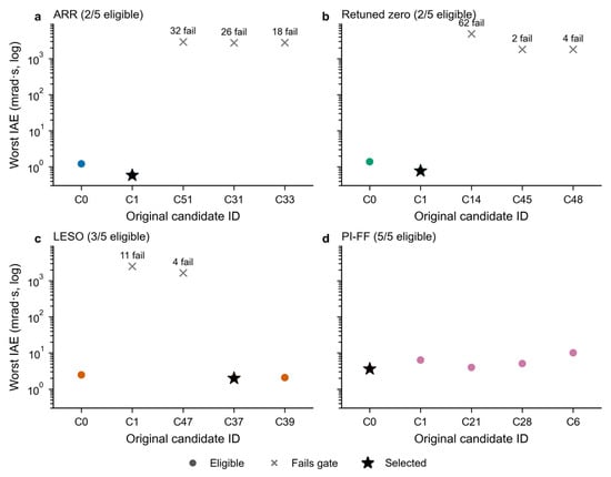
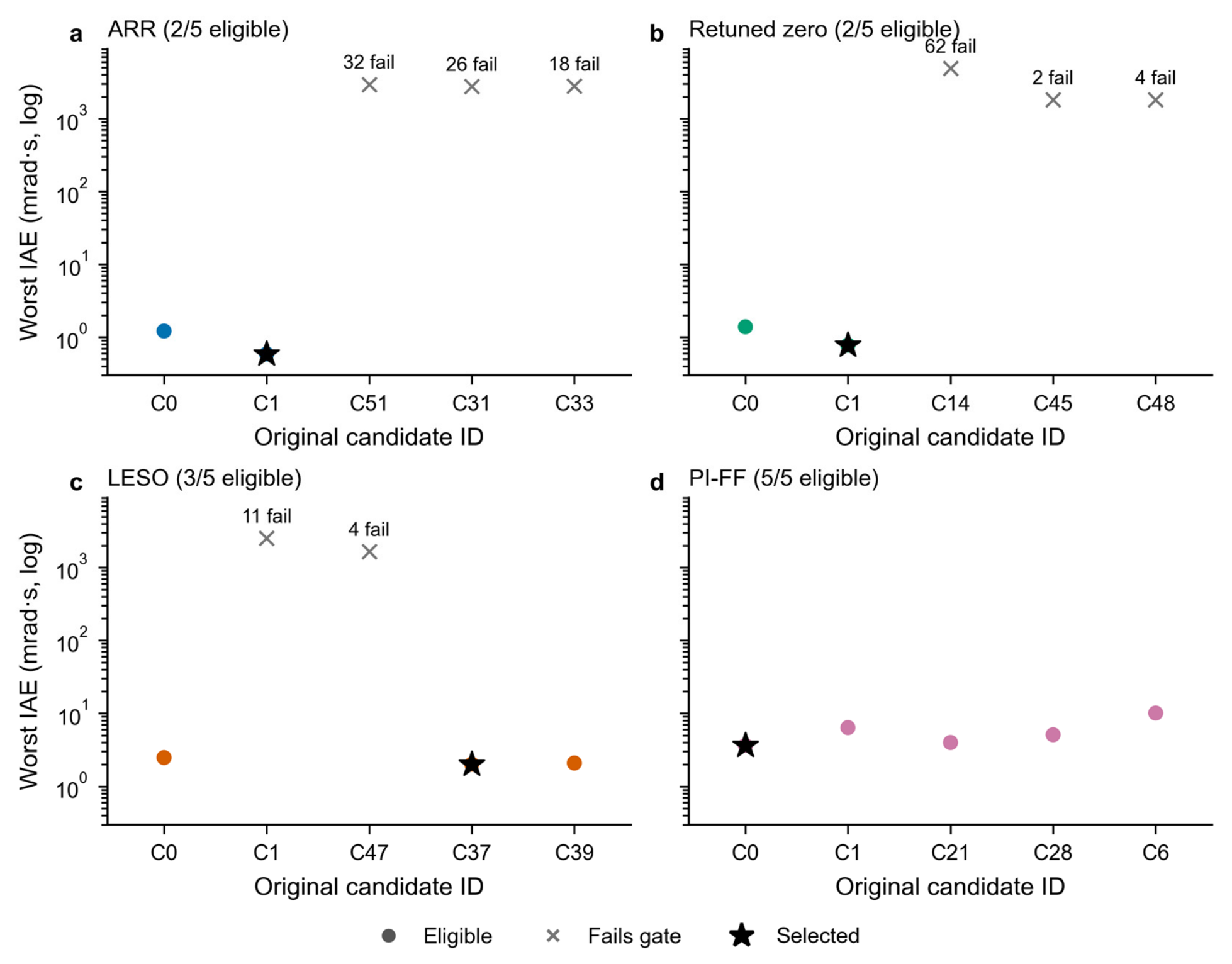
The nonlinear gate is necessary in addition to the local screen. The prior aggressive ARR candidate passes the local pole check but exhibits severe nonlinear failures. Within the five-candidate ARR pool, three candidates fail 32, 26, and 18 development cases, respectively. The complete 20-candidate record retains 159 failed development trajectories. These are development outcomes, not omitted validation failures; all selected parameters are frozen before the principal evaluation.
4.2. Operating Conditions and Data Separation
Principal evaluation consists of 1548 conditions for each of the five configurations, giving 7740 trajectories. Table 5 lists the full factorization. The first 780 conditions per configuration are retrospective protocol reassessments: their trajectories or operating demands had already been exposed during earlier control-design work. The remaining 768 conditions use 32 independently drawn motor-parameter vectors that were frozen but unopened during the final calibration. They test interior parameter transfer within the same average-dq model, not an independent physical model.
Table 5.
Principal evaluation matrix. The first four blocks are retrospective reassessments; only the 32-motor block is unopened in the final calibration. Five configurations yield 7740 principal trajectories.
The seven motion/load profiles include a smoothed position step, direction reversals, multi-frequency motion, signed-load recovery, and three two-second profiles with different hold, reversal, or chirped references. Load targets include positive and negative torques and recovery to zero. References and their derivatives are analytic; load transitions use finite ramps. Supplementary Section S4 gives every event time, amplitude, ramp duration, noise seed, and profile duration. Startup and every load transition remain inside the reported metric window.
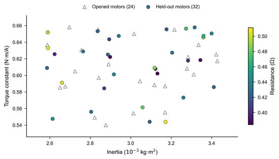
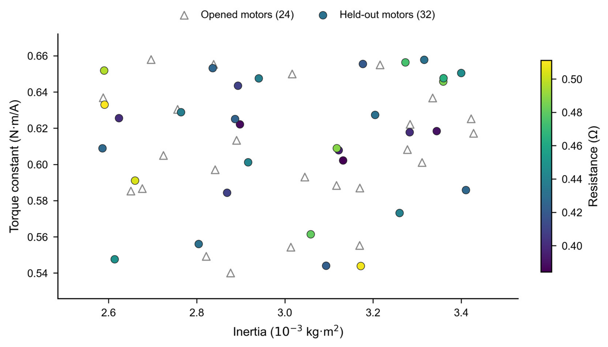
The fixed corners retain the physically linked flux/torque relation. The opened 24-motor set and unopened 32-motor set use independent uniform coordinates in the same five-dimensional box. Figure 1 shows their inertia/torque-constant projection with resistance encoded by color. The projection is a view of the inputs, not evidence that a two-dimensional scatter covers every possible parameter combination.
Figure 1.
Motor-parameter inputs. All 24 opened and 32 unopened draws are shown in an inertia/torque-constant projection, with resistance encoded by color. Marker shapes distinguish the two sets; this view is not a five-dimensional coverage guarantee.
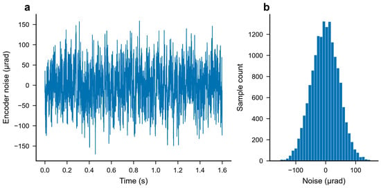
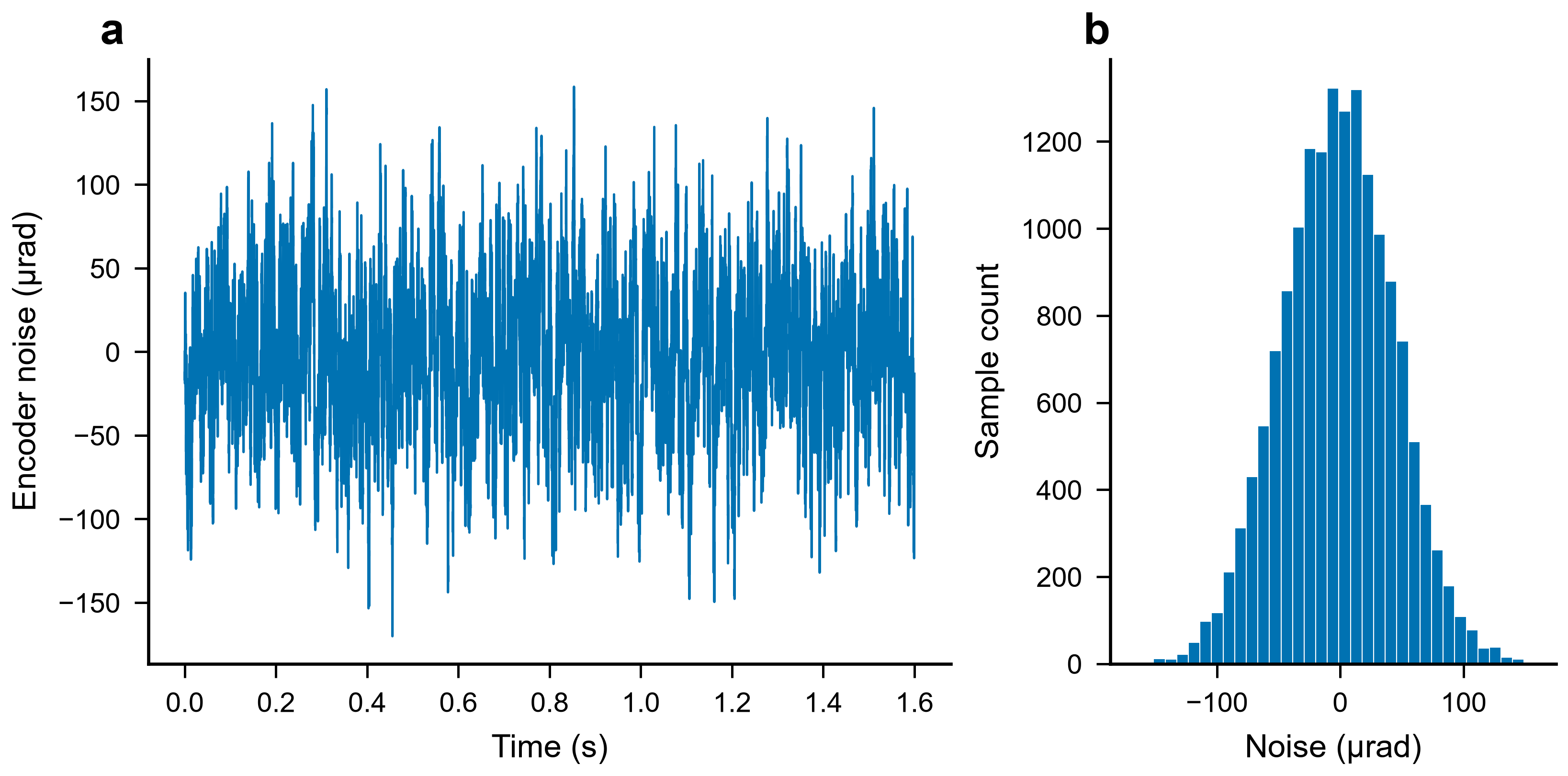
Encoder noise is bounded colored numerical noise, not a Gaussian sequence with the stated cap as its standard deviation. Its target combines the preceding sample with a Gaussian innovation, then limits both the increment and absolute amplitude. The default amplitude cap is . Identical sequences are supplied to paired methods. Figure 2 shows a complete calibration input and its empirical distribution; Supplementary Section S4 gives the generation formula.
Figure 2.
(a) Complete 16,000-sample encoder-noise input; (b) the empirical distribution for calibration seed 501. The declared cap is an amplitude bound, not a Gaussian standard deviation. No tails are removed.
4.3. Metrics and Paired Summaries
For pre-advance samples and the error , the full-window IAE and root mean square error (RMSE) are
Peak error is the maximum over the entire window. The terminal metric is the maximum absolute error over the final 1000 samples, corresponding to . The pass gates are feasibility screens for the declared numerical design objective, not derived stability margins.
For either generated reference or actual current, total variation is
The sum begins with the difference between the first two recorded samples. The command-slew audit separately includes the initialized previous command. The source tables also provide TV per second, obtained by dividing by , so profiles of different duration need not be compared solely by their accumulated totals. Command TV, actual-current TV, and current-tracking RMSE are kept distinct. None is an energy or semiconductor-loss measurement.
Each ARR/reference ratio is calculated within a common profile, delay, motor, and noise realization before aggregation. The reported paired median is not the ratio of two marginal medians. Fixed-profile/delay intervals resample complete shared-seed clusters while keeping the three corners together. Motor-draw intervals resample complete motors, retaining all conditions for each draw. Each uses 4000 percentile bootstrap resamples with a fixed generator seed. These are conditional summaries of this protocol, not universal success probabilities or independent populations of physical motors.
All five principal configurations are included in the absolute and relative tables. Sensitivity trajectories are reported separately rather than pooled into an attractive overall median. The accompanying metrics contain every evaluated condition, and the complete case matrix distinguishes current-loop, gain, noise/delay, and transport tests.
5. Tracking Repair and Incremental Correction Benefit
5.1. Absolute Performance Across the Principal Conditions
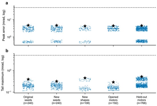
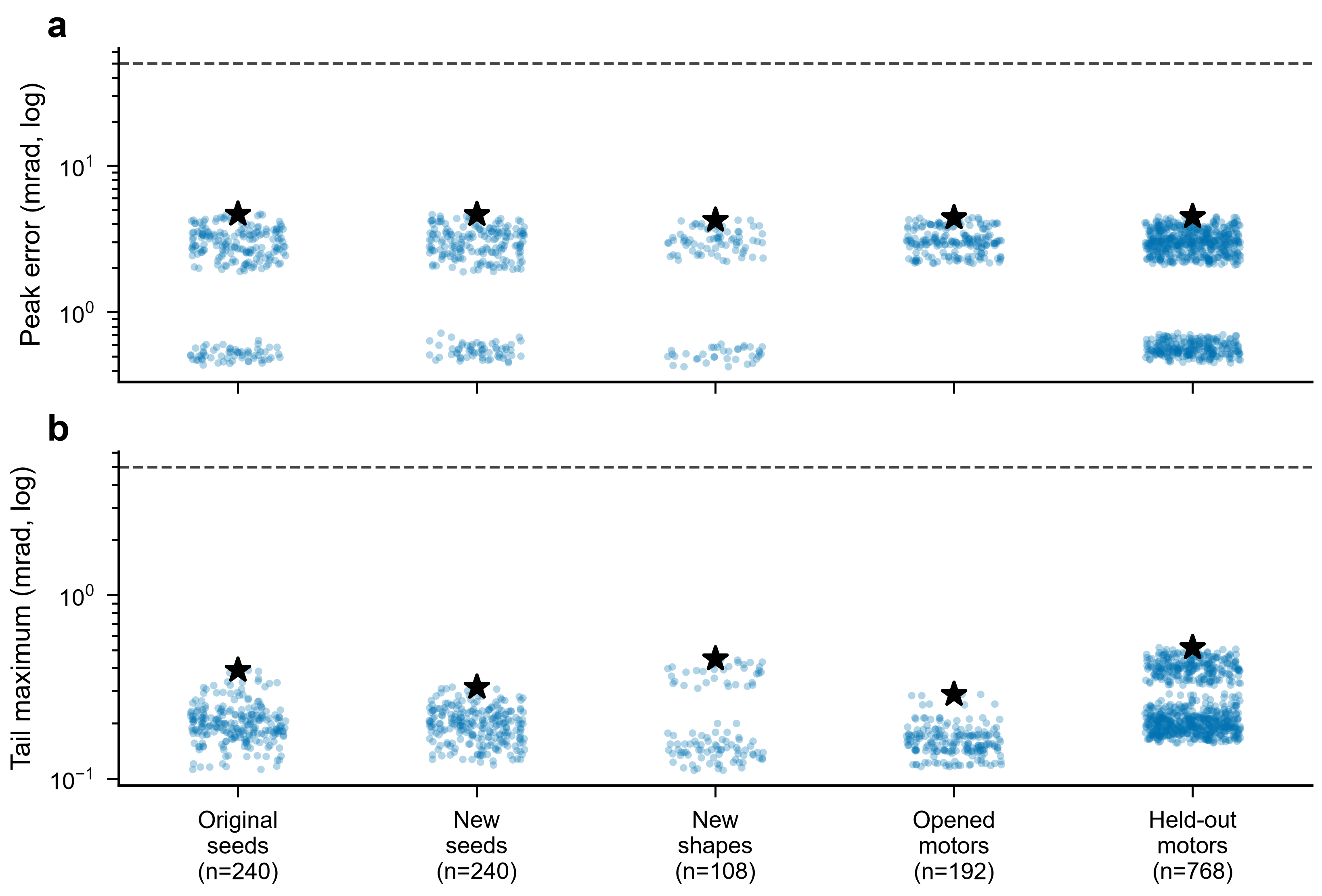
Every configuration passes all 1548 principal conditions. For ARR-LESO, the largest peak error is , and the largest final-window maximum is . Figure 3 displays every ARR peak and terminal value across the five principal blocks. Table 6 reports absolute outcomes for all five configurations, so successful tracking is not inferred only from a favorable ratio.
Figure 3.
(a) All 1548 ARR principal peak and (b) final-window errors by evaluation block. Horizontal jitter affects only position on the category axis. Stars mark maxima, not significance; dashed lines are the 50/5-mrad design gates. ARR denotes the arrival-residual reconciliation configuration.
Table 6.
Complete principal outcomes, per configuration, all passing. Integrated absolute error (IAE) and root mean square error (RMSE) are medians in and mrad; peak/tail are maxima in mrad; both total-variation (TV) columns are medians in A over the full windows.
The nine severe failures from the earlier narrow calibration are all repaired on retrospective retest. Within precisely those nine conditions, the worst peak decreases from to . This comparison concerns a changed parameter selection at the common condition. The failures cannot be presented as newly unseen tests or attributed solely to load switching: one earlier adverse trajectory already crossed the tracking gate before its first load event. Supplementary Section S7 retains their paired records and distinguishes the still earlier evidence.
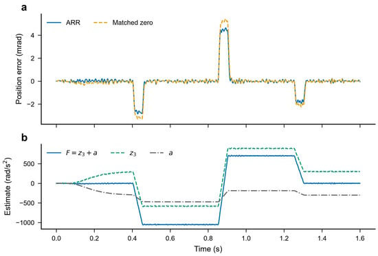
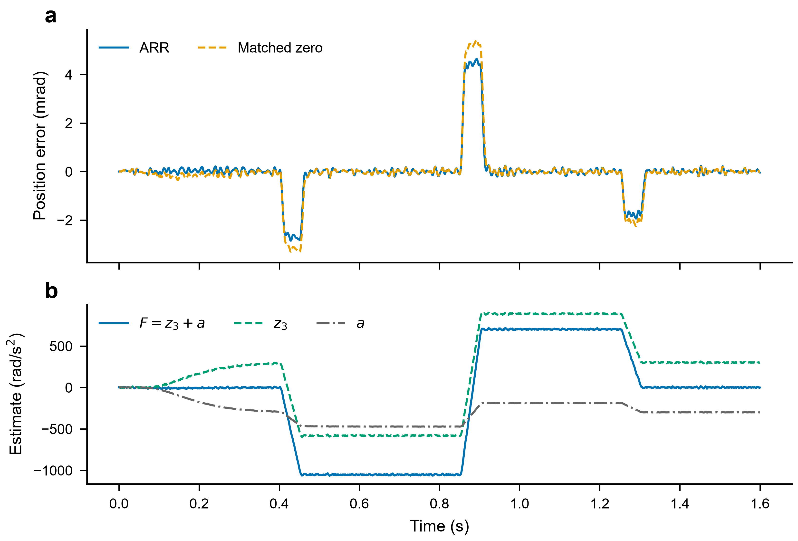
Figure 4 examines one predetermined signed-load trajectory at ten delay samples and a fixed parameter corner. The error remains on the milliradian scale through the positive, negative, and zero-load stages. Its lower panel separates , , and their sum. Their differing traces illustrate the implementation, while the total remains the disturbance estimate used by the predictor and compensation.
Figure 4.
Predetermined signed-load example, , corner 1, seed 401. (a) Upper panel compares ARR and matched-zero tracking error through all load changes; (b) lower panel shows and its separate coordinates. The components are not separately identified physical loads.
The improvement in reliability is associated with the nonlinear feasibility gate, not a new term inserted into the ARR equation. Figure 5 retains every candidate’s worst-case development IAE and failure count. Aggressive candidates can rank well on a narrow set yet fail badly at parameter vertices. Selecting only candidates that satisfy the absolute gates, before minimizing worst-case IAE, avoids turning a favorable average into the primary acceptance condition.
Figure 5.
All 20 nonlinear calibration candidates: (a) ARR (blue); (b) retuned predictive zero (green); (c) reference-preview LESO (orange); (d) PI-FF (purple). Each point uses 256 new cases; annotations retain failed-case counts. Colored circles indicate eligible candidates, grey crosses indicate failed candidates, and black stars identify selected candidates rather than statistical significance. The complete adverse range is shown on common logarithmic axes. Abbreviations: LESO, linear extended-state observer; PI-FF, proportional–integral control with feedforward; IAE, integrated absolute error.
All five final configurations successfully track the principal schedules, including the conventional PI reference. This outcome removes the previous severe-baseline-failure narrative. It also changes the scientific question: the evidence for ARR is its additional tracking correction at a stated variation cost, not exclusive possession of a workable controller.
5.2. Same-Parameter Ablation and Independently Calibrated References
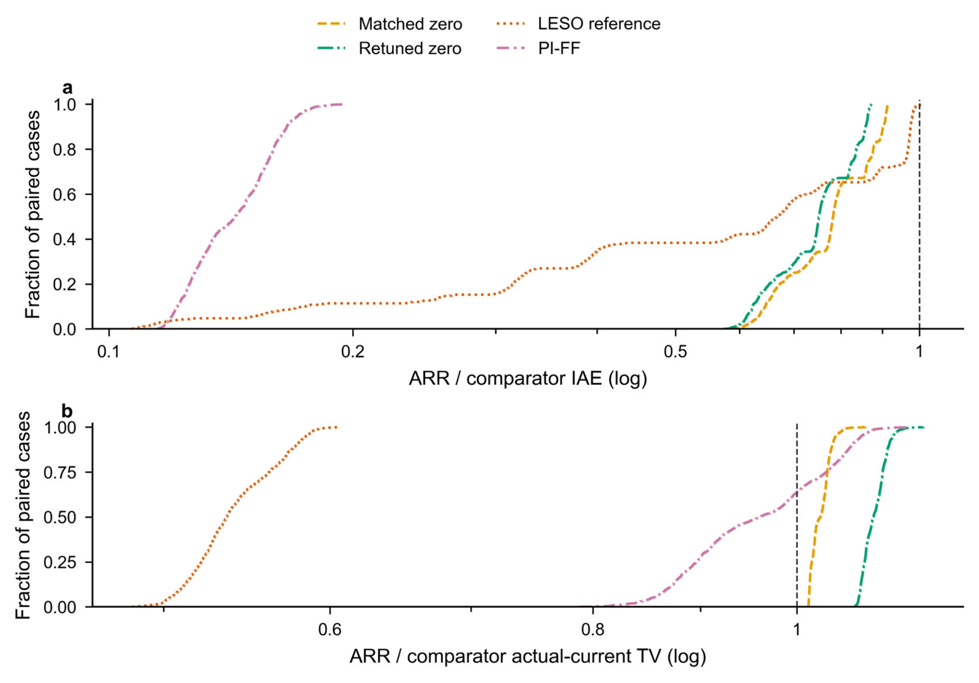
The cleanest comparison changes only the residual gain. Against matched zero, the median paired IAE ratio is 0.782411 across 1548 conditions, and ARR has lower IAE in every pair. The corresponding command-TV and actual-current-TV ratios are 1.020300 and 1.026101. Thus, the correction has a consistent IAE benefit in these conditions, while requiring slightly more current variation. The result is expressed as a trade-off rather than as simultaneous improvement of accuracy and smoothness.
Against the independently calibrated predictive zero-gain controller, the median paired IAE ratio is 0.751498, accompanied by an actual-current-TV ratio of 1.087501. The larger variation cost matters: independent calibration changes the point on the tracking/variation trade-off. Table 7 summarizes all paired comparisons. Matched zero identifies the added channel at fixed gains; the independently tuned zero-gain family checks whether gain selection in the existing predictive architecture eliminates its practical relevance.
Table 7.
Medians of per-condition paired ratios over 1548 pairs per row. Ratios below 1 favor ARR for that metric; these are not ratios of marginal medians.
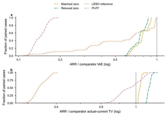
Figure 6 shows empirical cumulative distributions for all paired ratios, including the complete tails. The actual-current-TV distribution against matched zero lies above 1 for its median, whereas the IAE distribution lies below 1. The empirical cumulative distribution function (ECDF) describes the complete distribution of the evaluated paired outcomes.
Figure 6.
Empirical cumulative distributions of (a) all 1548 paired IAE and (b) actual-current-TV ratios per comparator. The reference line is 1. Fractions describe these evaluated cases, not future improvement probabilities; the ARR variation cost remains visible. TV denotes total variation.
The independent reference-preview LESO produces a median paired IAE ratio of 0.669205 in ARR/reference order, with lower ARR IAE in 1542 of 1548 cases. Six cases favor that reference. Its aggregate current variation is also different from ARR. This comparison combines the FIFO state rollout, reconciliation, and independently selected bandwidths; it does not identify the isolated residual effect or establish superiority to the full predictive ESO-ADRC of [22].
The PI-FF reference has a median paired IAE ratio of 0.143158 in ARR/reference order. Its conventional rate-aware integration and feedforward prevent the earlier long-delay PI anomaly from being used as an architecture-level argument. Its reference information and cascade structure still differ from the predictive observers. Consequently, the PI comparison provides an engineering reference under common command conditions, not another isolated ARR ablation.
On the unopened 32-motor block, the matched-zero median paired IAE ratio is 0.780675, with a conditional 95% motor-cluster percentile interval of [0.778137, 0.783025]. This is the 768-pair motor-holdout stratum, not the pooled 1548-pair median. All 768 ARR cases meet the absolute gates. The agreement with the pooled direction supports transfer across the sampled interior motors, while the fixed motion set, noise seeds, and plant family limit the interpretation of the interval.
6. Sensitivity and Adverse Operating Conditions
6.1. Current-Loop and Gain Sensitivity
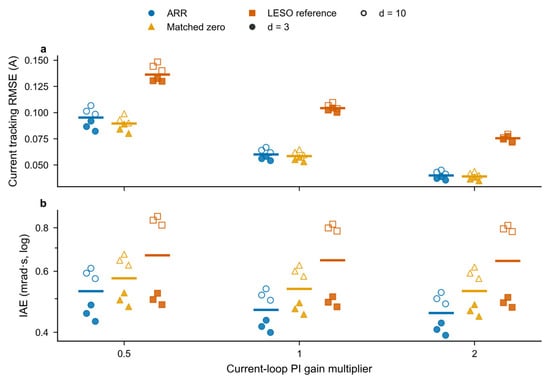
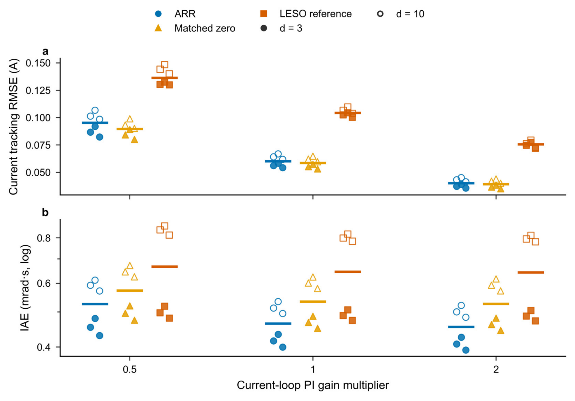
Finite current dynamics create a prediction mismatch because the predictor rolls out delayed references rather than measured actual current. The current-loop sensitivity therefore scales both PI gains by 0.5, 1, and 2, without giving the outer controller additional state information. It includes three fixed corners, delays of three and ten samples, and the signed-load profile for ARR, matched zero, and the reference-preview LESO. All 54 trajectories pass the declared tracking gates.
Figure 7 shows all individual IAE values and current-tracking RMSE for these cases. Increasing the current-loop gains reduces the actual-current/reference mismatch in this grid, while position IAE changes less strongly. This is consistent with a finite inner-loop contribution to the effective disturbance in Section 3. The tracking gates remain satisfied at the three tested scales; no claim of insensitivity to arbitrary electrical dynamics follows.
Figure 7.
All 54 current-loop sensitivity cases: (a) current-tracking RMSE; (b) IAE. The cases comprise three configurations, three PI scales, three corners, and two delays. Marker shapes identify methods and filling identifies delay. Bars are medians, not confidence intervals. The current-loop change is common to all methods. RMSE denotes root mean square error; PI denotes proportional–integral control.
A separate 144-trajectory ARR grid scales the residual gain by 0, 0.5, 1, and 2 and the observer bandwidth by 0.75, 1, and 1.25. It includes the four principal delays and three corners on the signed-load profile, with feedback bandwidth held fixed. All cases pass. Zero residual gain is included as a sensitivity point, not hidden as an inadmissible parameter. This finite sweep describes a neighborhood of working settings; it is not a continuously certified stability region.
A separate retrospective factorial diagnostic varies the physical motor vector, encoder noise, load, and current-loop gains in 16 matched backgrounds for four fixed input anchors. It evaluates the principal setting and a lower-bandwidth diagnostic setting, each with and without ARR, giving 256 trajectories. Supplementary Section S8 and Table S4 retain all outcomes. Under the principal gains, removing noise still leaves 14 of 32 ARR trajectories outside the tracking gates in these selected stress backgrounds. The correction benefit therefore cannot be explained or repaired by noise removal alone; current-loop, load, and parameter effects depend on the remaining background.
6.2. Noise and Delay Boundary
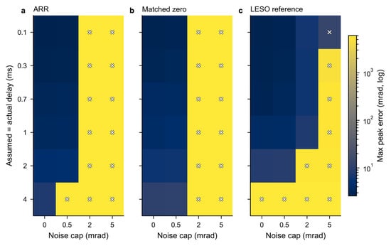
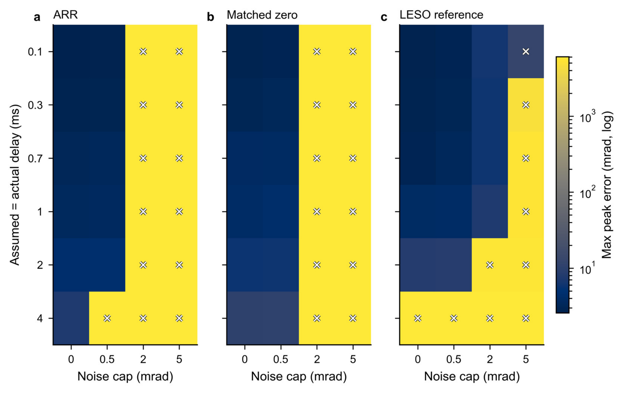
The noise/delay grid is intentionally broader than the principal design envelope. It tests the reversal profile at six exact delays, , and noise caps of 0, 0.0005, 0.002, and . Three seeds are used at each condition for ARR, matched zero, and reference-preview LESO. Figure 8 shows the worst peak among those three seeds in every cell; failed cells remain visible on the shared full-range scale.
Figure 8.
Noise/delay boundary for ARR, matched zero, and reference-preview LESO. Each cell reports maximum peak error over three seeds on a common full-range logarithmic scale. Crosses identify failed cells; cap denotes the encoder amplitude bound, not standard deviation.
ARR passes 34 of 72 noise/delay trajectories, matched zero 39, and the reference-preview LESO 44. In the noiseless cases, ARR passes all six tested delays. At the default cap, its three 40-sample-delay trajectories fail; at larger caps, severe errors become frequent. The largest ARR error in this noise grid exceeds . The failures identify a strong dependence on encoder-noise amplitude and prediction horizon.
The aggregate noise identity helps interpret, but does not fully predict, this boundary. The residual correction adds a same-sample encoder contribution to the LESO innovation path. A cap specifies an upper amplitude, not a noise spectral density or Gaussian standard deviation. Larger amplitude and longer prediction horizons alter the complete feedback response. The main-case correction benefit must therefore be read together with the adverse high-noise results.
The local frequency response and controlled noise removal in Supplementary Section S8 separate direct encoder injection from its propagated effect. At the diagnostic setting, both variants pass all 32 noiseless factorial backgrounds; with the recorded noise, ARR fails 7 of 32 and matched zero fails 2 of 32. These are deliberately selected retrospective backgrounds, not a population success rate. The local frequency response concerns inactive constraints and is not used to predict the saturated trajectories.
6.3. Synthetic Transport Mismatch
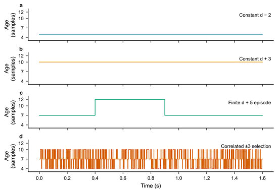
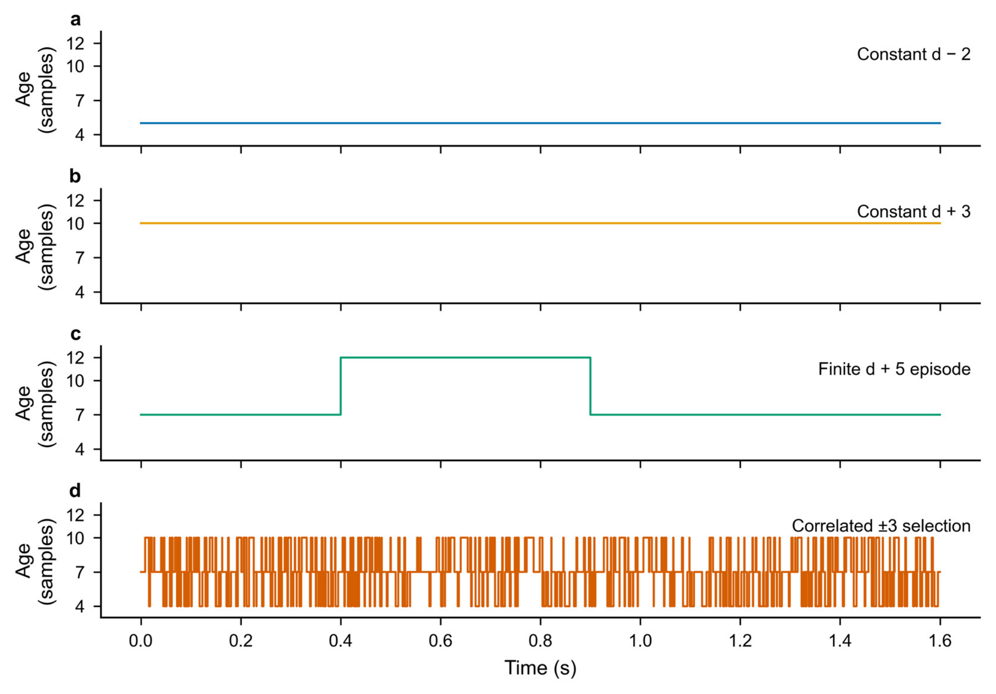
The transport tests retain a fixed declared FIFO inside the controller but perturb the delivered command age at the plant. Four synthetic modes are used: an age two samples smaller where feasible, an age three samples larger, a five-sample age increase during a fixed time block, and a correlated three-level age perturbation. Figure 9 displays complete age histories for a declared seven-sample delay. These are generated stress inputs, not recorded network or bus data.
Figure 9.
Complete synthetic delivered-command age inputs for declared , seed 981. Actual ages differ from the fixed controller-side queue assumption. The panels show (a) a constant age two samples below the declared delay; (b) a constant age three samples above it; (c) a five-sample age increase during a fixed time block; (d) correlated selection among ages three samples below, equal to, and three samples above the declared delay. These are generated stress histories, not measured network traffic.
Across two motion/load profiles, three declared delays, three corners, three seeds, and four modes, each of ARR, matched zero, and the reference-preview LESO has 216 trajectories. ARR passes 215, matched zero 216, and the reference-preview LESO 214. ARR’s failed case is the signed-load profile at declared , seed 983, with the temporary five-sample age increase; its peak error is . The other two failures belong to the reference-preview LESO. Table 8 summarizes the separate sensitivity blocks.
Table 8.
Passing/evaluated sensitivity counts. The 1062 cases include 102 failures and are not pooled into the principal tracking result.
The complete sensitivity record retains all 102 failures: 99 from noise/delay and three from transport. Actual-age histories identify the tested departures from the fixed controller-side FIFO.
Supplementary Section S8 further examines a distinct lower-bandwidth setting over 6912 conditions per method, with delays up to 40 samples and a persistent five-sample age increase. ARR fails 159 conditions and matched zero 65; these are separate from the 159 failed development trajectories in Section 4.1. In all 159 diagnostic ARR failures, amplitude and slew restrictions occur before the error first exceeds 0.05 rad. The 155 observed voltage-projection events occur later; four traces have none. This temporal ordering does not identify a unique cause, but it does exclude an earlier voltage-projection event in these particular records.
A further mechanism diagnostic fixes six previously observed cases before changing individual factors: four severe block-age cases from an unsuccessful aggressive gain setting and two low-input-gain FIFO cases near the peak-error threshold. The refined setting of Equation (22) and the aggressive setting defined in Supplementary Section S11 are both retained. The full factorization contains 160 trajectories. In the four selected severe cases, removing encoder noise, the temporary five-sample age increase, the residual update, or the software slew limit separately removes severe failure. These interventions diagnose the interaction; removing noise or the slew limit is not a revised operating condition. Table S14 reports the corresponding counts, and the complete factorization is supplied.
The first sustained slew restriction and amplitude clipping precede the first error crossing in a representative aggressive-setting trace; voltage projection occurs later (Table S15). Local analysis of the same observer, finite current loop and command histories gives 48 case-labeled models, using four distinct motor vectors. All inactive-limit, constant-age spectra remain inside the unit circle, with maximum radius 0.99977438 and a weakly damped mode near 39 Hz. The repeated motor anchors yield 32 distinct Jacobians, not 48 independent plant cases. The combined evidence supports a noise, delay-mismatch, residual-feedback and nonlinear-slew interaction in these selected trajectories; it does not support diagnosing them solely from a nominal pole instability. Supplementary Section S11 gives the model assumptions and numerical checks.
6.4. Residual-Horizon Calibration and Reassessment
An initial complementary diagnostic configuration separates the design-delay setting from the principal calibration. For the declared, fixed delay , its gains were set once as
The bandwidths are in and the residual gain is in . This configuration is reassessed retrospectively on the 1998 earlier ARR input conditions and the complete 6912-condition diagnostic grid of Supplementary Section S8. Its matched-zero configuration changes only to zero. Both use the same motor, reference, noise, realized command ages, and limits in each pair. The principal controller comparisons in Section 5 retain their independently calibrated settings.
At this initial setting, both configurations meet the two tracking criteria in all 1998 earlier conditions. The initial ARR configuration satisfied the terminal-error limit of 0.005 rad in all 6912 retrospective diagnostic conditions. The peak-error criterion of 0.05 rad was met in 6870 conditions (99.39%); the remaining 42 conditions exhibited a maximum peak error of 0.05210 rad. Table 9 reports the complete-cohort results, and Supplementary Section S10 provides the gain values and individual exception records.
Table 9.
Complete retrospective reassessment at the initial delay-dependent gains of Equation (21). Failures use the unchanged peak and terminal criteria; the IAE column is the median of the condition-wise ARR/matched-zero ratios, including every trajectory. Only the two matched configurations are compared here.
The median paired IAE ratios are 0.919712 and 0.921644 in the two cohorts. The corresponding actual-current-TV ratios are 1.007948 and 1.011236; command-TV ratios are 1.007499 and 1.009517. These matched comparisons quantify the correction benefit and variation cost at the revised gains. All trajectories are included, and the documented exploratory selections and adverse outcomes accompany the data.
The 42 peak exceptions motivated a finite refinement of the residual-horizon scaling, without changing the observer, feedback exponent, correction law or tracking criteria. Three first-pass exponents were rejected on 248 already observed conditions. A declared local bracket then selected by the frozen worst-normalized-error ranking. Table S12 retains all six candidate outcomes. The resulting fixed design-delay setting is
Complete reruns of both earlier cohorts give zero ARR failures in all 8910 conditions, including the original 198 failures and all 42 exceptions of Equation (21). Every previously passing ARR condition remains within the unchanged peak and final-window criteria. The largest peak in the 6912-condition grid is . Matched zero uses the same Equation (22) settings with ; its 576 failures in that grid remain in the comparison.
After these reruns, 1024 new inputs were frozen from 16 new motor vectors, two known motion/load profiles, delays of 1, 10, 20 and 40 samples, two encoder-noise caps, two new shared seeds, and FIFO or synthetic five-sample block-age perturbation. No parameter was changed after their evaluation. ARR meets the peak criterion in 1020 cases and the final-window criterion in all 1024; matched zero has 144 peak failures. The four ARR exceptions occur at delay 40 and the noise cap, with a worst peak of . Table S13 identifies every exception. Table 10 summarizes the complete results obtained with the refined setting in Equation (22), including all retained failures.
Table 10.
Complete results at the fixed refined setting of Equation (22). Peak and tail columns are ARR maxima in rad; failures count either unchanged tracking criterion. Ratios are medians of condition-wise ARR/matched-zero values, including every failure. The first two rows are retrospective, and the last uses new motor and noise realizations of the same model and two known profiles.
The new-input median paired IAE ratio is 0.921181, with a 95% motor-cluster bootstrap interval of [0.920754, 0.921472] from 10,000 resamples of the 16 complete motor groups. Its actual-current-TV ratio is 1.012865, quantifying the tracking–variation trade-off for the declared inputs. Equation (22) is a separately calibrated diagnostic setting; the principal comparisons retain their independently selected gains. The earlier regional certificates do not transfer to its changed delay-20 and delay-40 gains.
7. Interpretation and Applicability
The matched-zero comparison isolates the correction channel at fixed controller settings. Matched zero shares the observer and feedback bandwidths, queue rollout, preview, limiter, motor, and noise with ARR. Its only changed parameter is the residual gain. The paired IAE improvement therefore measures the added reconciliation channel within that implementation. Separately calibrated references answer a different question about finite-budget designs and should not replace this controlled ablation.
The design repair combines a common command-slew setting with nonlinear feasibility screening. The common software condition is a declared operating choice. The nonlinear calibration removes candidate settings with severe signed-load and parameter-vertex failures. The ARR mechanism remains the correctly indexed additional correction, whose benefit and current-variation cost are measured after the design conditions have been fixed.
ADRC combines unmodelled dynamics and external loading in a generalized disturbance, while practical discrete realizations use the limited input in the observer [25]. In the present delayed system, the observer uses the input released by its assumed FIFO; actual-current tracking and delivery mismatch therefore enter the aggregate residual budget. Under zero leakage and inactive bias projection, the equivalent disturbance coordinate is . The maximum principal bias magnitude is about , below the projection bound, so this aggregate representation describes the principal trajectories.
All principal trajectories have zero voltage-projection activation. The model includes a radial voltage limit to specify the drive consistently, but these cases do not validate operation on that limit. The actual-current variation results likewise describe a sampled signal: without a switching model or a loss calculation, they do not quantify inverter heating, switching loss, or energy efficiency.
Higher noise and persistent or blockwise delivery mismatch define a different regime from the principal fixed-delay comparison. Section 6.2, Section 6.3 and Section 6.4 retain those outcomes, the complete retrospective reassessment and the four new-input peak exceptions. The new mechanism diagnostic identifies a rate-limited interaction in selected aggressive-setting cases, whereas the low-input-gain exceptions occur around load reversal. These are distinct failure classes. The motor holdout and stress grids establish results for their declared inputs, rather than a continuous parameter-box or arbitrary-transport guarantee.
The signed residual budget identifies the discrepancies entering a stored prediction error, and the matched-zero comparison measures the incremental tracking effect of applying that residual. The regional analysis establishes bounded regulation for its specified initial and input sets; Section 5 and Section 6 quantify the wider transient response and its observed limits. These complementary results characterize the correction’s tracking–variation trade-off. Future work will examine noise-aware residual scheduling and less conservative sampled-delay bounds for longer and varying command delays.
8. Conclusions
ARR-LESO implements arrival-indexed residual injection before the observer and FIFO prediction updates. Its aggregate-state recursion, shared encoder-noise path and exact same-state command sensitivity describe how the correction acts. A projection-sector argument gives coupled regional boundedness and sufficient gain intervals, with interval-verified witnesses at twelve fixed operating points. The full-state initial sets and small input budgets make the scope of that result explicit. Four independently calibrated families and a same-parameter zero-gain configuration provide separate complete-controller and incremental-channel comparisons under common limits and finite current dynamics.
The constrained nonlinear calibration repaired the previously observed severe tracking failures. All five configurations pass 1548 principal conditions each; ARR’s worst peak and final-window errors are 4.691 and , including the 768-case unopened-motor block. The same-parameter comparison gives a median paired IAE ratio of 0.782411 and actual-current-TV ratio of 1.026101. This supports a measurable correction benefit with a modest variation cost in the stated regime.
The fixed-delay results quantify an incremental tracking benefit with a current-variation cost. At the separately refined delay-dependent setting, all 8910 earlier conditions pass, while four peak exceptions remain among 1024 new motor/noise inputs; the corresponding median IAE and actual-current-TV ratios are 0.921181 and 1.012865. The signed residual budget and noise/delay interventions further characterize aggregate correction and selected failure mechanisms. The regional bound supports regulation within its certified sets; the retained transient outcomes define the measured operating envelope.
Supplementary Materials
The following are available online at https://www.mdpi.com/article/10.3390/machines14111377/s1, Figures S1–S4 and Tables S1–S16 are described below. The Supplementary Materials specify controller timing, current-loop realization, references, noise, comparison laws, and retained adverse cases. They derive the sampled command sensitivity and regional boundedness result, and supply the factorial and larger-delay diagnostics, retrospective reassessment, and separate quadratic witnesses. The accompanying packages contain complete parameters, input and metric tables, verification routines, figure-source data, and representative raw traces; the full raw collections are retained separately. The refined-setting supplement additionally provides complete metrics for 19,868 paired-study trajectories, all six scalar-screen outcomes, the four new-input exceptions, and the signed residual decomposition. Supplementary Section S11 adds the complete 160-trajectory intervention study, first-event records and local-map diagnostics; Supplementary Section S12 lists the supplied numerical materials. Figure S1. Local encoder-noise responses at the diagnostic bandwidths, with residual gains zero and 100. Delays 1 and 40 are shown; the source includes delays 1, 10, 20, and 40. The two physical output channels are calculated separately. These equilibrium responses do not describe the saturated stress trajectories. ARR denotes arrival-residual reconciliation. Figure S2. All conditional changes in ARR IAE benefit, with 32 contrasts per factor and fixed gain set. Motor, noise, and load change from neutralized to recorded conditions; the current-loop factor changes both inner PI gains from one to two times their baseline. Horizontal bars are medians, not confidence intervals. The symmetric-log vertical axis has a linear threshold of 0.0001 rad·s. IAE denotes integrated absolute error. Figure S3. All 48 method/input cells in the diagnostic grid, with 288 conditions per cell. Color shows maximum peak position error on one logarithmic scale; cell labels give failures/288. Totals are 159/6912 ARR failures and 65/6912 matched-zero failures. Figure S4. First amplitude-limit and voltage-projection events relative to the first absolute position error above 0.05 rad in all 159 diagnostic ARR failures. The 155 traces with a voltage event are plotted; four missing events remain counted and unfilled. Event order is not a causal attribution. Table S1. Complete motion/load schedules. Step arguments are event time and amplitude; sums use increments. Load entries are successive targets reached through the stated ramps. Table S2. Noise seeds in every principal block. The same realization is shared by compared configurations within each condition. Table S3. Two fixed ARR settings used in the diagnostic study. Each matched-zero configuration changes only the residual gain to zero. The diagnostic setting is not a replacement selection. ARR denotes arrival-residual reconciliation. Table S4. All factorial noise/gain/method strata. Integrated absolute error (IAE) is in rad·s and includes failed trajectories. Each method/setting/noise stratum contains 32 trajectories; the four paired rows cover all 256 trajectories, including 72 failures. Table S5. Four retrospective factorial anchors. Zero-based motor indices refer to the 32-vector diagnostic input file. A1 and A2 share the same motor; they are not independent motor replicates. The matching full physical vectors and complete input arrays accompany the diagnostic supplement. Table S6. Complete diagnostic-grid failures and maximum peak error for every input cell. Each row has 288 conditions per method. Counts and full-range maxima include all failed trajectories. Table S7. Verified regional bounds for twelve fixed operating points. Each row conservatively groups the three independent load equilibria −3, 0, and 3 N·m. The position projection is an outer coordinate bound, not a sufficient initial condition. Command step is compared with 0.05 A; voltage is compared with 27.7128 V. Table S8. Alternative diagnostic gains. The final column is the conditional same-state raw-command sensitivity of Equations (18a) and (18b), not a closed-loop noise bound. Table S9. All 42 peak-criterion exceptions at declared delay 40. ID is the motor index in the original 32-vector diagnostic sample. Cap is the encoder amplitude bound; +5 block denotes the retained synthetic age increase. No exception is omitted. Table S10. Separate regional bounds at the alternative gains. Each row groups three independently verified constant-load equilibria. Position is an outer coordinate bound, not a sufficient initial condition. Numeric upper bounds are rounded upward. Table S11. Ten-term signed residual budget on 248 paired development conditions at Equation (22), using the exact identities in Supplementary Section S2. Entries are median per-trajectory root mean square (RMS) magnitudes in mrad, not error fractions. The cohort is an observed calibration diagnostic, not the independent new-input test. Table S12. Complete finite residual-exponent screening on 248 observed conditions per candidate. The second bracket was fixed after inspecting the first pass. Worst normalized error is the larger of peak/0.05 and tail/0.005. No candidate was changed after the new-input test. Table S13. All four ARR peak exceptions in the new-input test. Each uses profile hold, delay 40, encoder cap 0.005 rad and seed 3901. Draw is the zero-based new motor index. Full motor vectors and raw hashes are supplied. Table S14. Severe failures in the four selected block-age anchors. Each row has four trajectories. Noise removal, exact-FIFO substitution, inactive slew and zero residual gain are controlled interventions, not deployable improvements or relaxed formal criteria. Setting R is Equation (22); A is defined above. Table S15. First-event times in seconds for setting A with all original factors. Slew onset is the start of the first run of 50 consecutive clipped samples, not necessarily the first isolated rate clip. Error onset is the first absolute error above 0.05 rad. No missing event is assigned time zero. Table S16. Range of local spectral radii over the six labelled anchors at each fixed setting, residual state and constant actual age. The six labels contain four distinct motors. The 48 labelled configurations contain 32 byte-distinct Jacobians at central-difference scale 0.000001; three scales give 144 estimates, not 144 independent systems.
Author Contributions
Conceptualization, J.C. and Y.W.; methodology, J.C. and Y.C.; software, J.C. and Y.C.; validation, J.C., Y.C., X.H. and Y.W.; formal analysis, J.C. and Y.W.; investigation, J.C., Y.C. and X.H.; resources, X.H.; data curation, J.C., Y.C. and X.H.; writing—original draft preparation, J.C.; writing—review and editing, Y.C., X.H. and Y.W.; visualization, J.C. and X.H.; supervision, Y.W.; project administration, Y.W. and X.H.; funding acquisition, J.C. All authors have read and agreed to the published version of the manuscript.
Funding
This research was funded by the National Natural Science Foundation of China, grant number 62404182.
Data Availability Statement
The data derive from numerical simulations. The accompanying principal-study package provides model/controller sources, calibration and evaluation protocols, complete metric tables, paired summaries, figure-source arrays, and representative raw traces. Its complete principal-study raw archive contains 5120 development and 8802 evaluation traces, approximately 52 GB uncompressed. A separate diagnostic supplement provides the full factorial metrics and inputs, local frequency responses, complete larger-delay summaries, and event records described in Supplementary Section S8. The complete raw collections and earlier adverse records are retained separately and are available from the corresponding author upon reasonable request. The retrospective reassessment additionally retains all 17,820 raw trajectories, complete condition-wise metrics and gain-selection records, and the separate regional-certificate inputs. The refined-setting study retains 19,868 additional evaluation trajectories separately, with complete condition-wise metrics and raw hashes. Its compact supplement contains representative raw traces, rather than the entire raw collection.
Acknowledgments
The authors acknowledge financial support from the National Natural Science Foundation of China (Grant No. 62404182). During preparation of this manuscript, the authors used OpenAI Codex for manuscript revision, code correction and generation, literature searches, and technical formatting. The authors reviewed and edited the output and take full responsibility for the content of this publication.
Conflicts of Interest
The authors declare no conflicts of interest.
References
- Zheng, Y.; Xia, Y.; Li, K.; Zhou, H.; Precup, R.-E. Boundary-aware sliding prescribed performance control for PMSMs under compound uncertainties. Expert Syst. Appl. 2026, 304, 130786. [Google Scholar] [CrossRef] [Scilit]
- Liang, Y.; Wang, X.; Zhou, F.; Yin, Z.; Zhang, Y.; Shen, Y.; Zhao, H. Nonovershoot Oscillation-Free Tube-Based Prescribed Performance Speed Control for PMSM. IEEE Trans. Ind. Electron. 2026, 73, 1828–1836. [Google Scholar] [CrossRef] [Scilit]
- Qu, X.; Zhang, S.; Peng, C. Model-Free Adaptive Fast Integral Terminal Sliding Mode Control for Permanent Magnet Synchronous Motor with Position Error Constraint. World Electr. Veh. J. 2025, 16, 341. [Google Scholar] [CrossRef] [Scilit]
- Ding, F.; Liu, X. High-order fast fixed-time sliding mode single-loop control for PMSM with disturbance compensator. Control Eng. Pract. 2025, 164, 106509. [Google Scholar] [CrossRef] [Scilit]
- Cao, Z.; Mao, J.; Zhang, C.; Cui, C.; Yang, J. Safety-Critical Generalized Predictive Control for Speed Regulation of PMSM Drives Based on Dynamic Robust Control Barrier Function. IEEE Trans. Ind. Electron. 2025, 72, 1881–1891. [Google Scholar] [CrossRef] [Scilit]
- Xu, X.; Wang, L.; Zhang, Z.; Wu, Z. A novel robust control for permanent magnet synchronous motor integrating deadbeat predictive current control and sliding mode observer. Alex. Eng. J. 2025, 130, 57–67. [Google Scholar] [CrossRef] [Scilit]
- Zhang, Y.; Yang, P.; Zhang, J. Low complexity model predictive torque control of SPMSM based on a compensating sliding mode observer. Electr. Power Syst. Res. 2026, 257, 113022. [Google Scholar] [CrossRef] [Scilit]
- Thangarajan, K.; Soundarrajan, A. Performance comparison of permanent magnet synchronous motor (PMSM) drive with delay compensated predictive controllers. Microprocess. Microsyst. 2020, 75, 103081. [Google Scholar] [CrossRef] [Scilit]
- Zhang, C.; Zhang, L.; Wang, D.; Lu, K. A smith-predictor-assisted adaptive load disturbance rejection controller for speed variation suppression of PMSM drive. Int. J. Electr. Power Energy Syst. 2024, 155, 109666. [Google Scholar] [CrossRef] [Scilit]
- Pang, J.; Zhang, J.; Li, M.; Li, S. Time-varying command filters-based neural adaptive control with fixed-time prescribed performance for the PMSM with external disturbance and time delays. J. Frankl. Inst. 2025, 362, 107527. [Google Scholar] [CrossRef] [Scilit]
- Hu, M.; Ahn, H.; Chung, Y.; You, K. Speed Regulation for PMSM with Super-Twisting Sliding-Mode Controller via Disturbance Observer. Mathematics 2023, 11, 1618. [Google Scholar] [CrossRef] [Scilit]
- Choi, A.; Kim, H.; Hu, M.; Kim, Y.; Ahn, H.; You, K. Super-Twisting Sliding Mode Control with SVR Disturbance Observer for PMSM Speed Regulation. Appl. Sci. 2022, 12, 10749. [Google Scholar] [CrossRef] [Scilit]
- Liu, Y.-C.; Laghrouche, S.; Depernet, D.; Djerdir, A.; Cirrincione, M. Disturbance-Observer-Based Complementary Sliding-Mode Speed Control for PMSM Drives: A Super-Twisting Sliding-Mode Observer-Based Approach. IEEE J. Emerg. Sel. Top. Power Electron. 2021, 9, 5416–5428. [Google Scholar] [CrossRef] [Scilit]
- Sun, Z.; Tan, C.; Li, B.; Song, A.; Yu, P.; Hao, M. Dual Model Predictive Control Strategy of Direct-Drive PMSM Based on Sliding Mode Disturbance Observer. IEEJ Trans. Electr. Electron. Eng. 2024, 19, 527–534. [Google Scholar] [CrossRef] [Scilit]
- Zhufu, G.; Wang, S.; Wang, X. Finite time disturbance observer based sliding mode control for PMSM with unknown disturbances. Int. J. Robust. Nonlinear Control 2024, 34, 7547–7564. [Google Scholar] [CrossRef] [Scilit]
- Hong, J.; Lin, X.; Zhang, J.; Huang, W.; Yan, B.; Li, X. A composite sliding mode control with the first-order differentiator and sliding mode observer for permanent magnet synchronous machine. ISA Trans. 2024, 147, 489–500. [Google Scholar] [CrossRef] [Scilit]
- Yang, X.; Ge, Y.; Deng, W.; Yao, J. Command filtered adaptive tracking control of nonlinear systems with prescribed performance under time-variant parameters and input delay. Int. J. Robust. Nonlinear Control 2023, 33, 2840–2860. [Google Scholar] [CrossRef] [Scilit]
- Dai, Y.; Ni, S.; Xu, D.; Zhang, L.; Yan, X.-G. Disturbance-observer based prescribed-performance fuzzy sliding mode control for PMSM in electric vehicles. Eng. Appl. Artif. Intell. 2021, 104, 104361. [Google Scholar] [CrossRef] [Scilit]
- Gao, P.; Zhang, G.; Ouyang, H.; Mei, L. An Adaptive Super Twisting Nonlinear Fractional Order PID Sliding Mode Control of Permanent Magnet Synchronous Motor Speed Regulation System Based on Extended State Observer. IEEE Access 2020, 8, 53498–53510. [Google Scholar] [CrossRef] [Scilit]
- Li, L.; Zhou, W.; Bi, X.; Shi, X. Speed Estimation of PMSM Based on a Super-Twisting Slide Mode Observer. Machines 2022, 10, 681. [Google Scholar] [CrossRef] [Scilit]
- Zhang, X.; Hou, B.; Mei, Y. Deadbeat Predictive Current Control of Permanent-Magnet Synchronous Motors with Stator Current and Disturbance Observer. IEEE Trans. Power Electron. 2017, 32, 3818–3834. [Google Scholar] [CrossRef] [Scilit]
- Nahri, S.N.F.; Du, S.; van Wyk, B.J. Predictive Extended State Observer-Based Active Disturbance Rejection Control for Systems with Time Delay. Machines 2023, 11, 144. [Google Scholar] [CrossRef] [Scilit]
- Nahri, S.N.F.; Du, S.; van Wyk, B.J.; Nyasulu, T.D. Time-Delay Estimation Improves Active Disturbance Rejection Control for Time-Delay Nonlinear Systems. Machines 2024, 12, 552. [Google Scholar] [CrossRef] [Scilit]
- González, A.; Balaguer, V.; García, P.; Cuenca, Á. Gain-scheduled predictive extended state observer for time-varying delays systems with mismatched disturbances. ISA Trans. 2019, 84, 206–213. [Google Scholar] [CrossRef] [Scilit]
- Herbst, G. Practical Active Disturbance Rejection Control: Bumpless Transfer, Rate Limitation, and Incremental Algorithm. IEEE Trans. Ind. Electron. 2016, 63, 1754–1762. [Google Scholar] [CrossRef] [Scilit]
- Sariyildiz, E.; Hangai, S.; Uzunovic, T.; Nozaki, T.; Ohnishi, K. Stability and Robustness of the Disturbance Observer-Based Motion Control Systems in Discrete-Time Domain. IEEE/ASME Trans. Mechatron. 2021, 26, 2139–2150. [Google Scholar] [CrossRef] [Scilit]
- Boyd, S.; El Ghaoui, L.; Feron, E.; Balakrishnan, V. Linear Matrix Inequalities in System and Control Theory; SIAM: Philadelphia, PA, USA, 1994. [Google Scholar] [CrossRef] [Scilit]

Disclaimer/Publisher’s Note: The statements, opinions and data contained in all publications are solely those of the individual author(s) and contributor(s) and not of MDPI and/or the editor(s). MDPI and/or the editor(s) disclaim responsibility for any injury to people or property resulting from any ideas, methods, instructions or products referred to in the content. |
© 2026 by the authors. Licensee MDPI, Basel, Switzerland. This article is an open access article distributed under the terms and conditions of the Creative Commons Attribution (CC BY) license.