


Abstract
Inerter-based passive suspensions promise better ride comfort and road holding without active control, but their benefit depends on the network topology and on how the inerter is tuned. Four passive networks—a spring–damper baseline, a parallel inerter, a series tuned inerter damper (TID) and a two-branch network—are compared in a consistently parameterized passenger-car quarter-car model. Exact Root Mean Square (RMS) indices under ISO 8608 excitation are obtained from the Lyapunov equation, all networks are tuned with the same bounded optimization, and comfort–road-holding Pareto fronts are reported. Untuned inerters with typical literature values increased the RMS body acceleration by 56–105% when compared against the spring–damper baseline. Once tuned, at a static stiffness of 16 kN/m, the TID-based networks reduced it by 3.3% without loss of road holding. When road holding is relaxed to yield optimal comfort, RMS body acceleration is reduced by up to 9.1% (TID) and 16.8% (two-branch). The benefit grows with static stiffness: at 80 kN/m, the TID reduced body acceleration by 11.9% and dynamic tire load by 8.4% simultaneously. Two practical aspects are also quantified: a point-contact tire model overestimates the peak tire force on short obstacles by about 44% compared with a contact-patch filter, and the reflected rotor inertia of electromagnetic dampers must stay below about 9 kg for the adopted passenger-car parameters (16 kN/m) to avoid degrading comfort. Proper tuning, rather than the mere presence of an inerter, determines the benefit.
1. Introduction
Vehicle suspension systems play a fundamental role in automotive dynamics, serving as the primary interface between the road surface and the vehicle body. Their design directly governs three competing performance objectives that have defined suspension engineering for decades: ride comfort, road holding, and vehicle stability [1]. A well-tuned suspension must simultaneously attenuate road-induced vibrations transmitted to the vehicle occupants, maintain adequate tire–road contact forces to ensure safe handling, and preserve vehicle stability under dynamic maneuvers [2]. The inherent conflict among these objectives—a softer suspension favors comfort while a stiffer one favors handling—has motivated decades of research into passive, semi-active, and active suspension architectures [3,4].
Passive spring–damper suspensions remain the industry standard because of their simplicity, reliability and low cost, but their fixed parameters impose a performance ceiling [2]; semi-active [5,6] and active [7] systems relax it at the cost of energy consumption, complexity and expense (Section 2.1). These architectures are usually compared with the quarter-car model, which captures the essential vertical dynamics of a single wheel–body assembly with sufficient fidelity for comparative studies [8,9].
A transformative development in suspension design emerged with the formal introduction of the inerter as a two-terminal mechanical element by Smith [10]. The inerter is defined by its constitutive relationship, in which the force it develops is proportional to the relative acceleration between its terminals, with inertance as the constant of proportionality, making it the mechanical dual of a capacitor in electrical network analogies [10]. Critically, this inertance effect can be achieved with a device whose physical mass is orders of magnitude smaller than the equivalent inertia it represents, enabling significant dynamic benefits without the weight penalties associated with added mass [11]. The inerter thus completes the mechanical network trinity alongside the spring and damper, opening a rich design space of passive suspension topologies that were previously inaccessible [10]. Since its introduction, the inerter has attracted sustained research interest, with recent comprehensive reviews confirming its potential across a wide range of vehicular applications [12].
Inerters have since been incorporated into a wide variety of passive inerter–spring–damper (ISD) layouts [13,14,15], variable and nonlinear devices [16,17], and semi-active and active control schemes [18,19,20,21,22,23,24,25], while the nonlinearities of practical devices—friction, backlash and fluid effects—have been identified as a limitation of the predicted benefits [26,27,28,29]. These developments are reviewed in Section 2.2.
Despite this substantial body of work, several important limitations constrain the current state of knowledge. A significant portion of existing studies examine isolated configurations—typically a single inerter–spring–damper (ISD) topology or a specific control strategy—without systematic comparison against alternative inerter arrangements under consistent conditions [12]. The tuning of inerter-based suspensions, meaning the principled selection of spring stiffness, damping coefficient, and inertance to optimize a defined performance index, has received comparatively limited attention relative to the extensive literature on topology proposal [17,30]. Furthermore, many studies evaluate each performance index separately—the pioneering comparison of Smith and Wang [31] optimized ride comfort, tire grip and handling one at a time—rather than reporting the complete comfort–road-holding trade-off that is central to practical suspension design. The quarter-car model, despite its well-documented limitations, remains the most tractable framework for systematic comparative studies and has been widely validated as an appropriate tool for this purpose [8,32]. The closest study is that of Ramakrishnan et al. [1], who computed Pareto-optimal sets of six passive architectures for ride comfort, road holding and working space and found the inerter benefit to be more evident when the spring stiffness is held constant; the present work builds on that comparison, as detailed below.
This work addresses the identified research gap through a structured comparative analysis of four passive suspension networks—a conventional spring–damper baseline, a parallel inerter, a series inerter branch in the form of a tuned inerter damper (TID), and a two-branch network combining both—within a single, consistently parameterized quarter-car model. The contribution of this work is a systematic and internally consistent comparison of the four configurations studied. Performance is evaluated through stationary RMS indices obtained from the Lyapunov equation under ISO 8608 random excitation [33], complemented by ISO 2631-1 frequency-weighted acceleration, bump transients, and frequency responses [34]. Every configuration is tuned with the same bounded optimization procedure, and complete comfort–road-holding Pareto fronts are reported; this allows a fair comparison in which a richer network can never be penalized by an unfavorable choice of nominal parameters. In each case, the influence of the static suspension stiffness on the achievable benefit is quantified, showing when an inerter network is, and when it is not, worth its added mechanical complexity. Finally, two practical aspects of inerter suspensions are examined with the same model: the filtering of short obstacles by the finite tire contact patch, and the reflected rotor inertia of electromagnetic dampers, which acts as an unavoidable parallel inertance.
2. Literature Review
2.1. Vehicle Suspension Systems
The suspension system of a road vehicle fulfills two fundamental and often conflicting engineering requirements: isolating the vehicle body from road-induced disturbances to ensure occupant comfort and maintaining sufficient tire–road contact force to guarantee safe and predictable handling [1]. These objectives are governed by the dynamic properties of the suspension elements and their interaction with the sprung mass—representing the vehicle body and its contents—and the unsprung mass, which comprises the wheel, tire, and associated components [9]. The balance between these competing demands defines the core design problem that has driven suspension research for over a century.
Passive suspension systems, constituted by a linear spring and a viscous damper arranged in parallel between the sprung and unsprung masses, represent the conventional and most widely deployed solution in the automotive industry. Their appeal lies in their mechanical simplicity, high reliability, and absence of external power requirements [2]. However, the fixed nature of their parameters—spring stiffness and damping coefficient—means that their performance is necessarily a compromise optimized for a narrow range of operating conditions. Once designed, a passive suspension cannot respond to changes in road profile, vehicle loading, or driving dynamics, imposing an inherent performance ceiling that motivates the development of more sophisticated architectures [3]. Comparative studies have consistently demonstrated that while passive systems can be well-tuned for specific conditions, they are fundamentally outperformed by adaptive alternatives when evaluated across a broad range of excitation scenarios [2,4].
Semi-active suspension systems retain the passive spring but replace the fixed damper with a controllable dissipative element whose damping coefficient can be varied in real time based on measured system states [3]. The most prevalent implementations employ magnetorheological (MR) dampers, whose rheological properties change rapidly and reversibly in response to an applied magnetic field, enabling fast and precise damping force modulation [5,6]. Because semi-active systems only dissipate energy and require minimal external power—limited to the control electronics and the electromagnetic coil—they offer a favorable compromise between performance and energy consumption [5]. Classical control strategies for semi-active suspensions include skyhook control, which emulates a damper connected between the sprung mass and an inertial reference to minimize body acceleration, and groundhook control, which targets tire force minimization [22]. Hybrid strategies combining both objectives have been formulated to address the comfort-handling trade-off more effectively [19]. Frequency-based control approaches have further demonstrated that performance can be tailored across the frequency spectrum relevant to both ride and handling [20]. The practical effectiveness of semi-active systems has been extensively validated through both simulation and experimental testing, confirming their superiority over passive counterparts under realistic road conditions [5,6].
Active suspension systems replace or supplement the passive damper with a controlled actuator capable of generating forces in both directions, independently of the relative motion of the suspension endpoints [7]. This capability, in principle, allows simultaneous optimization of ride comfort and road holding without the fundamental compromises inherent to passive or semi-active designs. Active systems have been implemented using hydraulic, pneumatic, and electromechanical actuators, and have been controlled through a wide range of strategies, including linear quadratic regulation, H∞ robust control, MPC, and more recently reinforcement learning and deep learning approaches [4]. Despite their performance advantages, active suspensions carry significant penalties in terms of energy consumption, system complexity, cost, and potential failure modes, which have limited their adoption to high-performance and luxury vehicle segments [7]. Several studies have performed direct quantitative comparisons among passive, semi-active, and active architectures within unified simulation frameworks, providing consistent evidence of the progressive performance gains achievable at increasing levels of system complexity and cost [2,4].
2.2. Inerter-Based Suspension Design
2.2.1. Principle of the Inerter
The inerter was formally introduced by Smith [10,35] as a two-terminal mechanical element with the defining property that the force developed between its terminals is proportional to the relative acceleration of those terminals. Denoting the inertance as b (measured in kilograms), the constitutive equation of the inerter is
where F is the force applied at the terminals and and are their absolute accelerations [10]. In the force–current analogy, the inerter is the exact mechanical counterpart of the capacitor, while the spring corresponds to the inductor and the damper to the resistor [10]. The significance of this completion is that, before the inerter was introduced, passive mechanical networks could realize only the subset of admittances in which the mass element has one terminal connected to ground; with springs, dampers and inerters, any positive-real mechanical admittance can be synthesized [10,35,36].
Physically, the inerter can be realized through several mechanisms. The rack-and-pinion inerter converts linear relative displacement into rotational motion of a flywheel through a gear train, producing the required inertance effect [11]. The ball-screw inerter operates on an analogous principle using a helical mechanism and has been shown to achieve high inertance-to-mass ratios suitable for vehicle applications [37]. Fluid inerters exploit the inertia of a fluid column accelerated through a helical channel, offering a contactless implementation with inherently smooth force generation [27]. A critical practical advantage shared by all these realizations is that the effective inertance—the apparent mass amplification—can be made orders of magnitude larger than the physical mass of the device itself, enabling substantial dynamic benefits with negligible weight addition to the vehicle [11]. Experimental characterization of prototype inerter devices has confirmed that the ideal linear model provides a good first approximation, while also identifying nonlinear effects—including friction, backlash, and fluid nonlinearities—that must be incorporated for accurate performance prediction in real implementations [11,26,27,28,29].
A distinct realization path arises when the inerter effect is not introduced deliberately but emerges as a by-product of an electromechanical actuator. In electromagnetic dampers based on a rotary electric motor coupled to the suspension through a ball screw or a rack and pinion with a large transmission ratio, the rotational inertia of the motor is reflected at the suspension terminals as an inertance that cannot be neglected, so that the device behaves as an inerter with damping [38]. For a ball screw of lead ph driving a rotor of inertia Jm, the reflected inertance is (screw and nut inertia neglected). Because it scales with the square of the transmission ratio, the design choice that sets the achievable damping force also fixes the inerter effect, and the designer must trade damping authority against the inertance-driven increase in dynamic tire load [38]. This coupling is directly relevant to active and semi-active suspensions built around electric actuators, where the reflected motor inertia acts as a parallel inertance superimposed on any inerter introduced by design; its consequences are quantified with the present model in Section 6.7.
2.2.2. Automotive Applications of the Inerter
The application of inerters to vehicle suspension systems has been explored extensively since the element’s introduction, motivated by the theoretical prediction that passive networks incorporating inertance can achieve performance levels previously attainable only through active control [10,12]. The foundational suspension topologies incorporating inerters are derived from the ISD (inerter–spring–damper) framework, in which the three elements are interconnected in series, parallel, or hybrid arrangements to produce distinct frequency-domain admittance characteristics [13]. Early analytical studies demonstrated that specific ISD configurations could simultaneously reduce body acceleration and dynamic tire force compared to the conventional spring–damper baseline, resolving in part the classical comfort-handling conflict within a fully passive architecture [14,22,31].
Multi-objective optimization of passive ISD suspensions has confirmed that the introduction of inertance expands the achievable Pareto front in the comfort-handling performance space, providing superior trade-off solutions relative to optimized spring–damper systems [1]. The application of inerters to heavy-vehicle suspensions has shown particularly significant benefits due to the larger sprung-to-unsprung mass ratios characteristic of trucks and buses, where inertance effects are proportionally more influential [15]. Two-stage ISD configurations, in which a secondary inerter–spring–damper network is introduced in series with a primary stage, have been shown to extend effective vibration isolation to a broader frequency bandwidth while preserving road-holding performance [15]. Structural design studies have further examined the internal load paths and inertial interactions within ISD suspension assemblies, informing practical implementation guidelines [13].
The ride-comfort enhancement achievable through inerter-based passive networks has been formalized within the structure–immittance design approach, which directly synthesizes mechanical admittances to meet prescribed frequency-domain performance specifications [39]. Negative stiffness elements combined with inerters have been proposed as a means of further softening the effective suspension stiffness at low frequencies without compromising high-frequency isolation, demonstrating measurable ride quality improvements [40]. Variable inerter devices, whose inertance can be adjusted either passively through nonlinear mechanisms or actively through external control, have been introduced to overcome the single-operating-point limitation of fixed-inertance designs [16,17]. Nonlinear variable inerters have been characterized both analytically and experimentally, with results indicating that appropriately designed nonlinear inertance profiles can extend performance benefits across a wider range of excitation amplitudes [16].
The integration of inerters with semi-active and active control strategies has generated a distinct research thread examining hybrid passive–active inerter systems. Semi-active inerter suspensions, in which a controllable element modulates the effective inertance or the damping force in an inerter-equipped network, have been shown to outperform semi-active damping and passive inerters used in isolation [22,23]. Robust H∞ control applied to active inerter suspensions has demonstrated improved robustness to parametric uncertainty and road disturbance rejection compared to conventional active suspensions without inertance [18,25]. MPC of hydro-pneumatic inerter suspensions has shown effective multi-objective performance under realistic road profiles [19], and frequency-division control strategies have been proposed to leverage the inherent frequency-dependent characteristics of inerter networks for targeted vibration suppression in specific frequency bands [20]. Fuzzy logic control of two-stage ISD suspensions with variable inerters has further demonstrated the potential of intelligent control to adapt inertance scheduling to varying road conditions [29].
2.3. Quarter-Car Dynamic Modeling
2.3.1. The Quarter-Car Model in Suspension Analysis
The quarter-car model is the most widely employed analytical framework for the study and comparison of vehicle suspension systems, and its continued prevalence in the literature reflects a balance between physical fidelity and mathematical tractability [8,9]. The model represents one corner of the vehicle—comprising the sprung mass, ms; the unsprung mass, mu; the suspension elements connecting them; and the tire modeled as a linear spring, kt—subject to a vertical road displacement input, zr [8]. Despite abstracting away the roll, pitch, and yaw dynamics of the full vehicle, the quarter-car model captures the dominant vertical vibration modes that govern both ride comfort and road holding, making it an appropriate tool for comparative suspension studies and parameter optimization [9,32].
The two-degree-of-freedom quarter-car model produces a system of coupled ordinary differential equations whose frequency-domain transfer functions relate the road input to the key response quantities of interest. The sprung mass acceleration transfer function characterizes the ride-comfort behavior, as it directly determines the vibration energy transmitted to the vehicle occupants across the frequency range of human sensitivity, between 0.5 and 80 Hz, with peak sensitivity to vertical vibration near 4–8 Hz according to ISO 2631-1 [8,34]. The dynamic tire force transfer function—defined as the ratio of the dynamic component of the tire contact force to the static load—characterizes road holding, since reductions in this quantity indicate more consistent tire–road contact and therefore improved grip and handling [9]. The suspension working space, defined as the relative displacement between sprung and unsprung masses, constitutes a third performance metric that reflects physical packaging constraints and must remain within prescribed limits [1,32].
The quarter-car framework has been applied to evaluate passive, semi-active, and active suspension architectures under both deterministic and stochastic road excitation models. Deterministic analyses typically employ sinusoidal or step inputs to examine transient and steady-state response characteristics [9], while stochastic analyses model the road profile as a filtered white noise process characterized by an ISO road roughness class, enabling the computation of root-mean-square performance metrics under realistic driving conditions [8,32]. The linear quarter-car model has been validated against more complex multi-body vehicle models and experimental measurements, demonstrating that it provides accurate predictions of the primary vertical dynamics for the purpose of suspension comparison studies, while acknowledged limitations include the neglect of nonlinear damper characteristics and geometric effects [8,41].
2.3.2. Key Performance Metrics
The evaluation of inerter-based suspension configurations within the quarter-car framework requires the definition of consistent, physically meaningful performance indices that capture the essential trade-offs governing practical suspension design. The following metrics are adopted in this study, consistent with established practice in the suspension dynamics literature [1,2,8].
Ride Comfort Index. Occupant comfort is quantified through the root-mean-square (RMS) value of the sprung mass acceleration, , under a standardized stochastic road excitation, together with its ISO 2631-1 frequency-weighted counterpart [8,34]. For a linear model driven by a stationary random road, this RMS value equals the 2 norm of the corresponding transfer function scaled by the intensity of the road input [1].
Road Holding Index. Tire–road contact quality is assessed through the RMS dynamic tire force, i.e., the fluctuation of the vertical contact force about its static value, which is proportional to the dynamic tire deflection. Larger fluctuations imply intermittent loss of contact force and therefore degraded grip, braking and lateral force capacity [9]. Normalized by the static wheel load, it is the standard road-holding measure in quarter-car studies [2,22].
Suspension Working Space. The RMS relative displacement between the sprung and unsprung masses—the suspension stroke—must remain within physical limits imposed by bump-stop clearance and packaging constraints. This metric acts as a design constraint rather than an optimization objective and is monitored across all configurations to ensure practical feasibility [1,32].
Frequency Response Analysis. Beyond scalar RMS metrics, the frequency-domain transfer functions are examined directly to identify the natural frequencies, resonance peaks, and inter-resonance behavior of each configuration. This analysis reveals the mechanisms through which inerter addition modifies the system dynamics—including frequency shifting, peak attenuation, and the introduction of anti-resonance phenomena—and provides physical insight that complements the scalar performance indices [13,22,30].
3. Quarter-Car Dynamic Model
3.1. Conventional Quarter-Car Model
The quarter-car model represents the vertical dynamics of a single corner of a road vehicle through a two-degree-of-freedom lumped-parameter system (Figure 1). The sprung mass, ms, represents the portion of the vehicle body supported by the suspension at one corner, while the unsprung mass, mu, accounts for the wheel assembly, brake components and associated hardware [8,9]. The suspension consists of a linear spring, ks, and a viscous damper, cs, in parallel, and the tire is modeled as a linear spring, kt, acting between the unsprung mass and the road; tire damping is neglected in accordance with standard practice [9]. The model retains the two dominant vertical modes of the vehicle corner: body bounce, typically between 1 and 2 Hz, and wheel hop, typically between 10 and 15 Hz [8].
Figure 1.
Conventional quarter-car model: sprung mass ms, unsprung mass mu, suspension spring ks and damper cs, and tire stiffness kt. Blue arrows indicate the positive (upward) direction of the vertical displacements zs, zu, and zr(t), measured from their static equilibrium positions.
Denoting the vertical displacements of the sprung mass, unsprung mass and road surface by zs, zu and zr, measured from static equilibrium, Newton’s second law gives
Because gravity is balanced by the static deflections, it does not appear in Equations (2) and (3); the static wheel load, (ms + mu)g, is only needed to check tire–road contact (Section 5.4). The nominal parameters adopted in this study are listed in Table 1 and are representative of a passenger-vehicle corner [9,23]. With these values, the undamped natural frequencies are fb = 1.13 Hz (body bounce) and fw = 10.60 Hz (wheel hop), with damping ratios ζb = 0.31 and ζw = 0.26.
Table 1.
Nominal parameters of the quarter-car model.
3.2. Quarter-Car Model with Inerter Networks
3.2.1. Introduction of the Inerter Element
An inerter of inertance b connected between the sprung and unsprung masses develops the force , Equation (1). Unlike the spring, which stores potential energy, or the damper, which dissipates energy, the inerter stores kinetic energy proportional to the square of the relative velocity of its terminals [10,11]. It therefore resists changes in the relative velocity across the suspension, introducing an apparent inertia that can be made much larger than the physical mass of the device [11]. This frequency-dependent behavior is best described using the mechanical admittance, Y(s) = F(s)/V(s), of the suspension network, where V is the relative velocity across it: a spring contributes k/s, a damper c, and an inerter bs [35].
3.2.2. Inerter Network Configurations
Three inerter networks are considered, each placed between the sprung and unsprung masses in parallel with the conventional spring, ks, and damper, cs (Figure 2):
Figure 2.
Inerter networks placed in parallel with ks and cs, and their mechanical admittances Y(s): (a) parallel inerter (Configuration 2); (b) series inerter branch, i.e., tuned inerter damper (Configuration 3); (c) two-branch network (Configuration 4). Green: series branch with internal node zb.
Configuration 2—parallel inerter (Figure 2a): an inerter, b1, in parallel with the spring–damper unit. This is the simplest augmentation of the conventional suspension.
Configuration 3—series inerter branch (TID) (Figure 2b): an inerter, b2, in series with a spring, k2, and a damper, c2, that are themselves in parallel. This is the TID layout [42], whose branch behaves as a tuned absorber that does not require an added physical mass. The damper, c2, is essential: without it, the branch b2–k2 is undamped and introduces a lightly damped resonance at (Section 6.1).
Configuration 4—two-branch network (Figure 2c): the parallel inerter, b1, and the series TID branch combined, giving the richest network of the study [15,43].
3.2.3. Equations of Motion
For Configuration 2, the inerter force adds to the spring and damper forces, giving
The inertance thus enters the mass matrix both on the diagonal and as an off-diagonal coupling term, which is absent in the conventional model and modifies the eigenstructure of the system [10,22].
For Configuration 3, the series branch has an internal node of displacement, zb, between the inerter and the k2–c2 pair. The node is massless, so the inerter force must equal the force in the k2–c2 pair. The equations of motion are
Although zb carries no mass, Equation (7) is of second order in zb because of the inerter, so Configuration 3 has three degrees of freedom and six states. All four configurations can be written in the common form
where eu selects the unsprung mass equation and, for the most general Configuration 4,
To reach other configurations, the effect of inerter b1 can simply be set to 0 if needed. If the effect of inerter b2 is not required, the third row and column in M, Cd and K must be removed, followed by setting c2 = 0 and k2 = 0. These actions yield a properly conditioned differential equation set for all the configurations. The limit is continuous: with b2 = 10−3 kg, Configuration 3 reproduces the RMS indices of the baseline with the same cs to within 0.004%, and Configuration 4 those of Configuration 2 to within 0.002%, so the reduction introduces neither artificial stiffness or damping, nor numerical discontinuities. In the implementation, the series branch is removed (reduced model with k2 = c2 = 0) whenever b2 < 10−3 kg, which also covers designs at the lower bound, b2 = 0.
3.2.4. Physical Interpretation of the Inerter Term
At low frequencies, the inerter force, , is small and the suspension behaves as a conventional spring–damper. As frequency increases, the inerter becomes progressively stiffer in the admittance sense (Y = bs), so a parallel inerter transmits high-frequency forces from the wheel to the body; it also lowers the wheel-hop frequency because it adds apparent mass to both bodies. A series branch, in contrast, acts only near its own tuning frequency, approximately , where it behaves as a tuned absorber anchored between the two masses [42]. These two mechanisms explain why the benefit of an inerter depends strongly on how its parameters are chosen (Section 6).
3.3. Computational Formulation
Equations (9)–(11) constitute the physical (mass–damping–stiffness) model of the study, and all mechanical interpretations in the paper are based on them. A first-order form is introduced only as a computational device, for three specific reasons: (i) for the ISO 8608 road of Section 5.2.3, the road velocity is white noise, so with the road velocity as input the stationary RMS indices follow exactly from a Lyapunov equation, without time simulation or spectral integration; (ii) this exactness and speed are what make the tuning of Section 5.5 tractable, since it requires tens of thousands of evaluations of the performance indices; and (iii) the same matrices provide the frequency responses and an exact discrete-time integration of the bump and random-road responses. The explicit state-space matrices of Configurations 1 and 2 are given in Appendix A for verification.
Using road-relative coordinates r = q − zr1 and noting that a rigid-body translation does not deform the suspension elements (K1 = kteu, Cd1 = 0), Equation (9) becomes . With and input , the model is with
which has 2nq states (nq = 2 for Configurations 1–2 and nq = 3 for Configurations 3–4). The outputs , with Ft = kt(zu − zr), are linear combinations of the states, y = Cx; is the first row of the lower block of A. The frequency response from the road velocity to output yi is
and, when is white noise of intensity W (two-sided, E[u(t)u(t + τ)] = Wδ(τ)), the stationary covariance, P, of the states solves the Lyapunov equation, from which the RMS value of every output follows directly:
Hi(jω) = Ci(jωI − A)−1B
This exact formulation is used for all RMS indices and for the optimization of Section 5.5 [1,30]; the intensity, W, of the ISO 8608 road is derived in Section 5.2.3.
4. Suspension Configurations
This section summarizes the four suspension architectures compared in this study (Figure 3). All configurations share the same sprung mass, unsprung mass, tire stiffness and static spring stiffness, ks, so that observed performance differences are attributable exclusively to the suspension network and its tuning.
Figure 3.
Quarter-car models of the four configurations: (a) C1, baseline spring–damper; (b) C2, parallel inerter b1; (c) C3, series inerter branch (TID) b2–(k2‖c2); (d) C4, two-branch network. All share ms, mu, kt and ks. Green indicates the additional series inerter branch.
4.1. Configuration 1—Baseline Suspension (Spring–Damper)
The baseline is the conventional passive suspension of Section 3.1, with suspension force . With ks fixed, its only design parameter is cs. The nominal value of Table 1 gives the reference against which all results are expressed.
4.2. Configuration 2—Parallel Inerter
The parallel inerter adds to the suspension force, Equations (4) and (5). Its design parameters are {cs, b1}. Because the inerter adds apparent mass to both bodies, it lowers both natural frequencies—most markedly the wheel-hop frequency—and couples the unsprung mass motion directly into the body at high frequency (Section 3.2.4) [10,22].
4.3. Configuration 3—Series Inerter Branch (TID)
The series branch b2–(k2‖c2) adds one degree of freedom, Equations (6)–(8). Its design parameters are {cs,b2,k2,c2}: the ratio k2/b2 sets the tuning frequency of the branch, while c2 controls the depth and bandwidth of its absorbing action [13,42]. Earlier formulations of this layout without c2 produce an undamped branch resonance; including c2 makes the branch a genuine tuned inerter damper.
4.4. Configuration 4—Two-Branch Network
Configuration 4 combines the parallel inerter b1 with the series TID branch, giving the five design parameters {cs,b1,b2,k2,c2} and three degrees of freedom (six states). Since Configurations 1–3 are special cases of Configuration 4 (b1 = 0 and/or b2 = 0), its optimum can never be worse than theirs; this nesting is exploited in the optimization (Section 5.5) and serves as a consistency check of the results. Network-synthesis theory indicates that such higher-order passive networks can approach the performance of low-authority active suspensions within specific frequency bands [10,18,31,36].
4.5. System Parameters
Table 2 consolidates the parameters of the four configurations: the fixed parameters, the nominal (untuned) inerter values used in Section 6.1, and the bounds applied in the tuning of Section 5.5. The static stiffness, ks, is held fixed, because it is dictated by ride height and static deflection rather than by dynamic performance [31]; its influence is studied separately in Section 6.6. The lower bound, cs ≥ 200 N·s/m, keeps a residual main damper in every design.
Table 2.
System parameters, nominal (untuned) inerter values and optimization bounds.
The inertance ratio β = b/ms quantifies the apparent mass of the inerter relative to the sprung mass. The nominal values of Table 2 (β = 0.27 and 0.40) are typical of those reported in the literature [1,22,30] and correspond to devices whose physical mass is of the order of a few kilograms [11,37]. They are deliberately left untuned in Section 6.1 to show the consequences of choosing inerter parameters without optimization.
5. Simulation Methodology
5.1. Simulation Platform and Verification
All computations are implemented in MATLAB R2026b as a modular, toolbox-free script library, so that the results can be reproduced with a basic MATLAB installation or with GNU Octave. Models are built from Equation (12); frequency responses are evaluated from Equation (13); RMS indices are computed exactly from the Lyapunov equation, Equation (14), solved in Kronecker form. Time responses are obtained by exact zero-order-hold discretization of the state equations, Ad = eAΔt, with the input held constant over each step; this avoids solver tolerances altogether for linear time-invariant models.
The numerical tools were verified independently: (i) the Lyapunov RMS values agree with direct numerical integration of over 10−3–103 Hz to within 0.15%; (ii) the average RMS values of a Monte Carlo ensemble of 50 independent 30 s road realizations agree with the Lyapunov values to within 0.7%, whereas the RMS value of a single finite record is itself a random estimate: individual 60 s records scatter around the Lyapunov value with a standard deviation of about 2%, so deviations of the order of 3% (Section 6.4.3) are expected, and all comparisons between configurations are therefore based on the exact Lyapunov values; (iii) the implemented ISO 2631-1 Wk filter reproduces the tabulated weighting factors to within 0.1%; (iv) steady-state swept-sine amplitudes agree with the analytical frequency response to within 0.4%; and (v) the Welch spectra of the generated road profiles match the ISO 8608 target (Figure 4b).
Figure 4.
Road inputs: (a) speed-hump profile, zr, and its velocity, ; (b) ISO 8608 spatial PSD of Classes B, C and D: target (dashed) and Welch estimate of the generated 600 s profiles (thin lines).
5.2. Road Excitation Profiles
Three road excitation profiles are employed, each probing a different aspect of the response [9,44].
5.2.1. Bump Profile
A localized obstacle, such as a speed hump, is modeled as a versine (raised-cosine) profile
whose time derivative, the input of the state-space model, is
The versine is continuously differentiable and avoids impulsive velocity inputs [9]. A hump of height A = 0.05 m and length L = 3.7 m crossed at v = 8 m/s (29 km/h) is used, giving a traversal time of 0.46 s and a dominant excitation near 2.2 Hz, between the body-bounce and wheel-hop frequencies. The geometry was chosen so that the tire remains in contact with the road for every configuration; an obstacle that produces tire lift-off would violate the linear tire model (Section 5.4.3). The simulation lasts 3 s from zero initial conditions.
The point-contact idealization applies the geometric profile of Equation (15) directly at the tire–road interface. A real tire envelops an obstacle over a contact patch of finite length, lp, which attenuates the wavelengths shorter than lp and therefore the high-frequency content of the excitation. To account for this, the effective road input is obtained by averaging the geometric profile over the contact length,
and its time derivative is used as the model input. For the passenger-car tire of this study, the static deflection is δst = F0/kt = 17.8 mm; the geometric chord m for a rolling radius R ≈ 0.31 m is an upper bound of the patch length, since the tread flattens rather than penetrating the road, and lp = 0.15 m is adopted as the nominal value. Because the effect of the patch depends on the ratio lp/L, a second, short obstacle is also considered: a cleat of height 20 mm and length 0.25 m crossed at 8 m/s, representative of a pavement joint or small debris. The sensitivity of both responses to lp between 0 (point contact) and 0.30 m is analyzed in Section 6.4.2.
5.2.2. Sinusoidal Input
A sinusoidal road, zr(t) = Asinsin(2πfexct), with Asin = 0.01 m, is used only to verify the frequency-domain model in the time domain. For each test frequency the response is simulated for 15 cycles, the first five are discarded as transient, and the steady-state amplitude is compared with |H(j2πfexc)| (Section 5.1).
5.2.3. Random Road Profile (ISO 8608)
The random road profile is the primary excitation for the comparison. Following ISO 8608 [33], the road elevation is a stationary zero-mean Gaussian process with one-sided spatial Power Spectral Density (PSD):
where n is the spatial frequency (cycles/m), n0 = 0.1 cycles/m, w = 2 and Gd(n0) depends on the road class. At constant speed v the temporal frequency is f = nv, and the temporal PSDs of road elevation and road velocity are
so that, for w = 2, the road velocity is white noise. Its two-sided intensity, used in Equation (14), is therefore
Time-domain realizations are generated by sampling Gaussian white noise of variance W/Δt for and integrating it to obtain zr. Three road classes are considered: Class B (Gd(n0) = 64 × 10−6 m3), Class C (256 × 10−6 m3, reference condition) and Class D (1024 × 10−6 m3), at v = 20 m/s. Figure 4 shows the bump profile and the agreement between the target PSD and the Welch estimates of 600 s realizations. The spectrum of Equation (18) with w = 2 is a mathematical idealization: integrated white road velocity is not a stationary elevation process and has unbounded variance, whereas the road-relative responses of the vehicle (body acceleration, suspension deflection and dynamic tire load) are stationary with finite variance, which is all the Lyapunov indices require. The generated realizations are band-limited by the record length, T, and the time step, Δt = 10−3 s (Table 3), i.e., they contain temporal frequencies between 1/T and 500 Hz; at 20 m/s and T = 600 s, this corresponds to spatial frequencies between 8.3 × 10⁻⁵ and 25 cycles/m, which contains the 0.011–2.83 cycles/m band of ISO 8608 [33].
Table 3.
Simulation settings.
5.3. Initial Conditions and Simulation Settings
All time-domain simulations start from zero initial conditions, x(0) = 0, i.e., from static equilibrium. For random-road simulations, the first Twarm = 5 s are discarded so that RMS values are computed from stationary data [32]. The settings are summarized in Table 3.
5.4. Performance Indicators
Three primary indicators are used, consistent with Section 2.3.2 [1,2,8]; together with the transient indicators of the bump test, they are summarized in Table 4. RMS values under random excitation are computed exactly with Equation (14); the time-domain definitions below are used for the bump response and for verification.
Table 4.
Performance indicators and evaluation conditions.
5.4.1. RMS Body Acceleration (Ride Comfort Index)
Lower values indicate better comfort. The frequency-weighted acceleration, aw, is obtained by passing through the ISO 2631-1 Wk filter (band limiting: 0.4–100 Hz, a–v transition at 12.5 Hz and upward step between 2.37 and 3.35 Hz) [34]; it is computed exactly by augmenting the state-space model with a realization of Wk before solving Equation (14).
5.4.2. Suspension Deflection
The available travel to the bump stop is dmax = 0.08 m. Designs with drms > dmax/3 are treated as infeasible, so that three-sigma excursions remain within the physical travel [1,30]. The peak deflection under the bump is recorded as a transient check.
5.4.3. Dynamic Tire Load
Ft is the fluctuation of the contact force about the static wheel load, F0 = (ms + mu)g; the quarter-car sprung mass already represents one corner, so no further division is required. The normalized value is also reported [2,30]. Tire contact is lost when F0 − Ft < 0; the minimum of F0 − Ft is monitored in every bump simulation to confirm the validity of the linear tire model. With the upward-positive displacements of Figure 1, a positive Ft corresponds to tire extension, so the compressive normal force is F0 − Ft and lift-off occurs when Ft > F0.
5.5. Tuning Procedure
Each configuration is tuned over its design vector, p (Table 2), with ks fixed. Because comfort and road holding conflict, the tuning is posed as an ε-constraint problem:
Sweeping ε between the minimum achievable Frms and the Frms of the pure-comfort optimum traces the Pareto front of each configuration. The selected design of each configuration is the solution with ε equal to the Frms of the nominal baseline, i.e., the best comfort attainable without any loss of road holding with respect to Configuration 1. Two extreme designs are also computed: the comfort optimum, J1 (min arms subject only to the travel constraint), and the road-holding optimum, J3 (min Frms subject to the travel constraint).
The problem is solved with the Nelder–Mead simplex method (MATLAB fminsearch) [45]. Bounds are enforced through the change of variables pi = plb,i + (pub,i − plb,i)(1 + sinsi)/2 and the constraints through an exterior quadratic-plus-linear penalty. To reduce the risk of local minima, each problem is solved from several random starts, and the nesting of the networks is exploited in both directions: the optimum of a simpler network seeds the richer one (e.g., C3 → C4 with b1 = 0), and the optimum of the richer network, reduced to the parameters of a simpler one, seeds it again. Each Pareto front is computed with a forward and a backward warm-started sweep, retaining the better solution at each point. As a result, a richer network is never reported to be worse than a network it contains. This nesting enforces consistency between the networks but does not, by itself, demonstrate global optimality. The settings were: the midpoint of the bounds and four to six uniformly distributed random starts per problem (three times as many for C4), in addition to the seeds provided by the nested networks and by neighbouring Pareto points, with the random generator seeded with 2026 and 2027 for ks = 16 and 80 kN/m; each problem is finished by a polishing run from the best point. The penalty adds 104Σgi2 + 102Σgi to the objective, where gi are the normalized constraint violations; the fminsearch tolerances are TolX = 10−8 and TolFun = 10−10, with MaxFunEvals = MaxIter = 3000nv (nv: number of design variables); and each Pareto front uses 12 values of ε, equally spaced between the minimum achievable Frms and the Frms of the comfort optimum. To verify repeatability, the selected and comfort-optimal designs of all configurations at 16 and 80 kN/m were recomputed from ten independent sets of random starts, without warm starts. The objective values were reproduced to within 0.2% in every case, and no run found a better design than those reported. The design parameters were reproduced to four significant digits, except for the selected TID designs at 16 kN/m, whose optimum is flat: there, cs varied between 200 and 380 N·s/m and b2 between 160 and 200 kg for changes in arms below 0.2%.
6. Results and Comparative Analysis
The results are organized to separate the effect of the network topology from the effect of its tuning. Section 6.1 evaluates the inerter networks with the nominal, untuned values of Table 2; Section 6.2 presents the tuned designs and Pareto fronts; Section 6.3 and Section 6.4 analyze the frequency and time responses of the tuned designs; Section 6.5 consolidates the indicators; Section 6.6 examines the influence of the static stiffness; and Section 6.7 discusses the reflected inertia of electromagnetic dampers. Unless stated otherwise, results refer to ks = 16 kN/m, ISO Class C road at 20 m/s, and percentage changes are computed relative to the nominal baseline C1.
6.1. Inerter Networks with Untuned Parameters
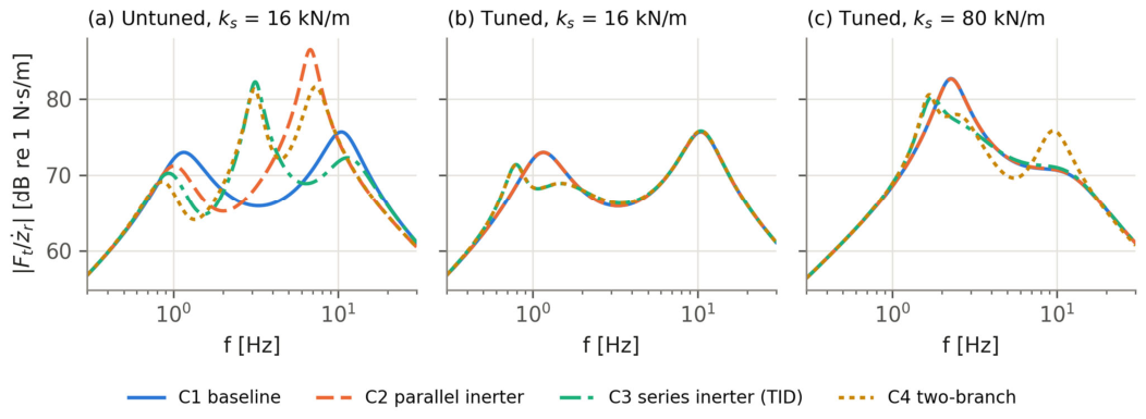
Table 5 and Figure 5a and Figure 6a show the response of the four configurations when the inerter parameters take the nominal values of Table 2. All three inerter networks perform markedly worse than the baseline: the RMS body acceleration increases by 105% (C2), 56% (C3) and 82% (C4), and the RMS dynamic tire load by 73%, 5% and 39%, respectively.
Table 5.
Performance and modal data with the nominal (untuned) inerter values of Table 2 (ISO Class C, 20 m/s).
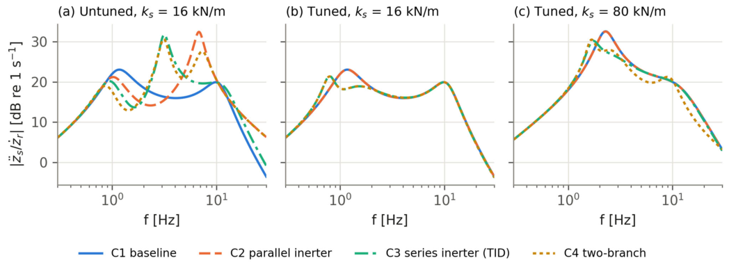
Table 6.
Tuned designs. Values of b ≈ 0 indicate that the corresponding inerter is not used by the optimum. At 80 kN/m, the reference, C1, keeps the damping ratio of the nominal design (ζb = 0.34, cs = 3354 N·s/m) and defines the road-holding constraint; the selected C1 (cs = 3409 N·s/m) is the best C1 under that constraint and differs from the reference by less than 0.02% in arms and Frms.
Figure 6.
Frequency response from road velocity to dynamic tire force for the same three parameter sets as Figure 5.
The modal data explain this behavior. The parallel inerter b1 = 80 kg adds apparent mass to the wheel and lowers the wheel-hop frequency from 10.60 Hz to 6.79 Hz, while its damping ratio drops from 0.26 to 0.11; the wheel-hop resonance is thereby shifted into the frequency range of high human sensitivity and amplified (peak of 41.7 vs. 14.2 (m/s2)/(m/s)). In addition, the inerter couples the wheel motion directly to the body, so the acceleration response no longer rolls off at high frequency (Figure 5a). In Configurations 3 and 4, the series branch with b2 = 120 kg and k2 = 40 kN/m is tuned to Hz, far from both natural modes of the vehicle, and it creates an additional, lightly damped mode at 3.13 Hz (ζ = 0.10) that dominates the response. Without the branch damper (c2 = 0), this mode would be undamped by the branch itself and the resonance would be even sharper. These results show that adding an inerter with arbitrarily chosen parameters can be strongly detrimental, and they motivate the systematic tuning of Section 5.5.
6.2. Tuned Designs and Pareto Fronts
Figure 7a shows the Pareto fronts of the four configurations for ks = 16 kN/m, and Table 6 lists the tuned designs. The fronts confirm the nesting of the networks: every richer network dominates the networks it contains. At the road-holding end, all fronts converge (the minimum Frms is 778 N for C1–C2 and 773 N for C3–C4, a difference of only 0.7%). The fronts separate progressively toward the comfort end: the comfort-optimal designs reduce arms by 3.8% (C2), 9.1% (C3) and 16.8% (C4) with respect to the comfort-optimal baseline, at the cost of a higher dynamic tire load.
Figure 7.
Comfort–road-holding Pareto fronts (arms vs. Frms, ISO Class C, 20 m/s, drms ≤ dmax/3) for (a) ks = 16 kN/m and (b) ks = 80 kN/m. Stars: selected designs (minimum arms without loss of road holding with respect to the reference, C1). In (a), the C2 star coincides with C1 and the C4 star with C3.
The selected designs—the best comfort without loss of road holding—are of particular practical interest. For C2, the optimum is b1 ≈ 0: at this static stiffness, a parallel inerter cannot improve comfort without degrading road holding, so C2 reduces to the baseline. For C3, the optimizer places the series branch at Hz, close to the body-bounce frequency, with a large inertance (b2 = 199 kg, β = 0.66) and transfers most of the damping from the main damper (cs at its lower bound) to the branch damper, c2. The branch then acts as a tuned absorber on the body-bounce mode and reduces arms by 3.3% at equal Frms; C4 converges to the same design (b1 ≈ 0). All tuned designs satisfy the travel constraint with a wide margin (drms ≤ 16.8 mm vs. dmax/3 = 26.7 mm).
For the stiffer suspension (ks = 80 kN/m, Figure 7b), the picture changes qualitatively. The baseline has no trade-off left—the same cs minimizes both indices—and the TID design dominates it in both objectives: arms and Frms decrease by 11.9% and 8.4%, respectively. The two-branch network exploits the parallel inerter as well (b1 = 33 kg) and reaches a 16.6% reduction in arms at the tire load of the baseline, whereas the parallel inerter alone yields only 0.1% under the same constraint.
6.3. Frequency Response of the Tuned Designs
Figure 5b,c and Figure 6b,c show the frequency responses of the selected designs, and Table 7 summarizes their modal properties. At ks = 16 kN/m, the TID splits the body-bounce mode of the baseline (1.13 Hz, ζ = 0.31) into two modes at 0.79 Hz (ζ = 0.14) and 1.42 Hz (ζ = 0.50), the classical signature of a tuned absorber. The body-bounce peak of the acceleration response falls from 14.2 to 11.8 (m/s2)/(m/s), and the response between 1 and 2 Hz is attenuated by up to about 5 dB, while the wheel-hop region (10.60 Hz) is practically unchanged. This explains why the gains at this stiffness are modest: the remaining acceleration energy is dominated by the wheel-hop band, which the selected design cannot attenuate without increasing the dynamic tire load.
Table 7.
Modal characteristics of the selected designs. Modes 1 and 2 of C3/C4 result from the splitting of the body-bounce mode by the TID branch; C2 coincides with C1 at both stiffnesses within 0.1% and is omitted.
At ks = 80 kN/m, the body-bounce mode of the baseline is at 2.26 Hz and produces a pronounced acceleration peak of 42.3 (m/s2)/(m/s). The TID again splits it into two well-damped modes (1.70 Hz and 2.52 Hz) and reduces the peak to 32.2, which also lowers the tire force peak from 13.5 to 10.3 kN/(m/s) (Figure 6c). The two-branch network adds the parallel inerter, which lowers the wheel-hop frequency to 9.45 Hz and reduces the acceleration above about 10 Hz, at the cost of a higher tire force peak in the wheel-hop region.
6.4. Time-Domain Response
6.4.1. Bump Response
Figure 8 shows the response to the speed hump, and Table 8 lists the transient indicators. With the tuned designs, C3 and C4 reduce the peak body acceleration from 3.37 to 3.02 m/s2 (−10.4%), the peak body displacement from 54.8 to 50.8 mm, and the peak suspension deflection from 43.1 to 40.4 mm. The post-bump oscillation is slower, as expected from the lower first mode (Table 7), and the settling time increases slightly (1.69 s vs. 1.77 s).
Figure 8.
Response to the speed hump (contact-patch filtered input, lp = 0.15 m): body displacement, zs; suspension deflection; body acceleration; and dynamic tire force for (a) untuned and (b) tuned designs (ks = 16 kN/m). The grey line is the road profile; the dotted red line marks tire lift-off, Ft = (ms + mu)g.
Table 8.
Transient response to the speed hump (A = 50 mm, L = 3.7 m, v = 8 m/s, lp = 0.15 m), ks = 16 kN/m.
The untuned networks show a mixed transient picture: C2 reduces the peak acceleration (2.52 m/s2), because the hump excites mainly frequencies around 2 Hz, where its acceleration response is low (Figure 5a), whereas C3 and C4 increase it to 4.34 and 4.23 m/s2 and exhibit a long-lasting oscillation at the branch mode near 3.1 Hz. This illustrates that a single deterministic test can rank configurations differently from the stochastic indices and that both must be considered. In all cases, the minimum contact force remains above 1850 N and the peak deflection below 45 mm, confirming that the tire stays on the ground and the suspension remains within its travel.
6.4.2. Influence of the Tire Contact Patch
Figure 9 and Table 9 compare the point-contact input with the contact-patch filtered input of Equation (17). For the speed hump (L = 3.7 m), whose wavelength is more than twenty times the patch length, the filter has a negligible effect: with lp = 0.15 m, the peak body acceleration and peak tire force change by only −0.2% and −0.2%, and even with lp = 0.30 m by less than 1%. The results of Section 6.4.1 are therefore insensitive to the contact model. For the short cleat (L = 0.25 m), the situation is different. The point-contact model predicts a peak tire force of 3357 N, reached in compression as the tire climbs the cleat, whereas the patch-filtered input with lp = 0.15 m gives 2334 N (−30.5%); the peak body acceleration decreases by 18.8%. The minimum contact force, which occurs during the rebound behind the cleat, is much less sensitive to the contact model (880 N with point contact and 1050 N with the filter), so the tire remains in contact in both cases. In other words, the point-contact model overestimates the peak tire force by about 44% for an obstacle of this size.
Figure 9.
Influence of the tire contact patch: (a) effective profile of the cleat (20 mm × 0.25 m) for several patch lengths; (b) peak dynamic tire force and (c) peak body acceleration relative to the point-contact model for the speed hump and the cleat (tuned C1 and C3, ks = 16 kN/m). The dotted line marks the nominal lp = 0.15 m.
Table 9.
Peak transient responses with point contact and with the contact-patch filter (tuned designs, ks = 16 kN/m, 8 m/s). C2 and C4 coincide with C1 and C3, respectively.
The effect is practically the same for the baseline and for the tuned TID design (Figure 9b,c), so the contact model does not change the comparison between configurations; it changes the absolute level of the transient loads on short obstacles. Since the result depends strongly on lp between 0.1 and 0.2 m, the patch length should be measured (e.g., from a static footprint) when the model is applied to a specific tire.
6.4.3. Random Road Response
Figure 10 shows representative 3 s excerpts of the body acceleration and dynamic tire load on the ISO Class C road. The untuned networks visibly amplify both signals, in agreement with Table 5, whereas the tuned designs produce time histories that differ from the baseline only slightly, mostly through a reduction in the slow body motion. The RMS values estimated from the 60 s simulations (1.348 and 1.315 m/s2 for C1 and C3) differ from the exact Lyapunov values by about 3% because of the finite record length, while the 50-realization Monte Carlo average agrees with them to within 0.7% (Section 5.1). Since this record-to-record scatter is of the same order as the 3.3% improvement of the selected design, the comparison relies on the exact Lyapunov values rather than on individual records.
Figure 10.
Representative 3 s excerpt of the response to the ISO Class C road at 20 m/s: sprung mass acceleration (top) and dynamic tire load (bottom) for (a) untuned designs with nominal parameters from Table 2 and (b) tuned designs. Legends give the RMS values of the full 60 s records.
6.5. Consolidated Performance Comparison
Table 10 consolidates the indicators of the selected designs. Because the models are linear and the ISO 8608 road velocity is white noise, every RMS index scales exactly with , Equation (20): the values for Classes B and D are exactly one half and twice those of Class C (e.g., the arms of C1 equals 0.695, 1.390 and 2.779 m/s2 for Classes B, C and D), and the relative ranking and percentage changes are therefore independent of the road class and of the vehicle speed. This invariance is a property of the adopted idealization—a linear model excited by an unbounded ISO 8608 spectrum with w = 2—and not a general property of inerter suspensions on real roads, whose spectra are band-limited and may depart from w = 2. This property, rather than a numerical coincidence, explains the constant ratios between road classes; road-class sensitivity becomes meaningful only for nonlinear models or roads with w ≠ 2.
Table 10.
Consolidated performance of the selected designs (ks = 16 kN/m, ISO Class C, 20 m/s). Classes B and D scale every RMS value by exactly 0.5 and 2.
The comparison shows that, at the nominal suspension stiffness of 16 kN/m, the 3.3% reduction in RMS body acceleration is obtained under the strict requirement of unchanged road holding. This modest gain reflects the inherent conflict between isolating the vehicle body from road disturbances and controlling tire-load fluctuations to maintain road contact. When the road-holding constraint is relaxed, the comfort-optimal TID and two-branch configurations reduce RMS body acceleration by 9.1% and 16.8%, respectively, relative to the comfort-optimal spring–damper baseline, but at the expense of increased dynamic tire loads (see Table 6). Thus, the practical value of an inerter depends on the acceptable comfort–road-holding compromise: the 3.3% improvement alone does not establish that the additional mechanical complexity is warranted, whereas larger comfort gains may motivate its consideration where increased tire-load fluctuations are acceptable.
6.6. Influence of the Static Stiffness
Since ks is fixed by the ride-height requirements of each vehicle, the analysis was repeated for ks between 10 and 120 kN/m, tuning every configuration for the comfort optimum, J1, and the road-holding optimum, J3 (Section 5.5). The variation interval for ks was selected to match sprung mass natural frequencies between 0.9 and 3.2 Hz. Since only ks was varied, while the masses, the tire stiffness and the excitation remained those of the passenger-car corner of Table 1, this study is a sensitivity analysis with respect to the static stiffness: it reveals a trend, but it does not represent other vehicle classes (sports cars, trucks or off-road vehicles), which also differ in mass ratio, tire stiffness, damping, suspension travel and excitation spectra. Figure 11 and Table 11 report the improvements relative to the equally tuned baseline. For comfort, the ranking C4 > C3 > C2 holds at every stiffness, and the gains of C2 and C3 grow with ks: from 3.8% and 9.1% at 16 kN/m to 8.9% and 14.8% at 120 kN/m. The road-holding benefit is negligible for soft suspensions (below 1% up to 25 kN/m) but reaches 8.8% at 80 kN/m and 12.6% at 120 kN/m for the TID-based networks, whereas the parallel inerter contributes little to road holding (at most 1.4%, at 120 kN/m). These trends agree with the observation of Smith and Wang [31] that inerter networks are most beneficial for stiffly sprung vehicles, in which the conventional damper alone cannot control the body-bounce mode without transmitting large forces.
Figure 11.
Influence of the static stiffness, ks, on the improvement achieved by the inerter networks relative to the equally tuned baseline, C1: (a) comfort-optimal designs (J1, reduction in arms); (b) road-holding-optimal designs (J3, reduction in Frms). In (b), C3 and C4 coincide.
Table 11.
Comfort-optimal (J1) and road-holding-optimal (J3) results versus static stiffness. Percentages are changes relative to the tuned baseline C1 at the same ks (negative = improvement).
6.7. Implications for Electromagnetic Dampers
In an electromagnetic damper, the reflected rotor inertia, , acts as a parallel inertance across the suspension (Section 2.2.1), i.e., the device is a Configuration 2 network whose inertance is fixed by the motor and the transmission rather than chosen freely. Table 12 shows that ball-screw leads of 5–20 mm combined with rotor inertias of the order of 10−4 kg·m2 produce equivalent inertances from a few kilograms to several hundred kilograms, i.e., of the same order as—or larger than—the inerter values considered in this study. To assess the consequences, the parallel inertance b1 of Configuration 2 was swept from 0 to 200 kg with the main damper at its reference value (Figure 12).
Table 12.
Equivalent inertance [kg] of a ball-screw electromagnetic damper for illustrative rotor inertias, Jm, and screw leads, ph (screw and nut inertia neglected).
Figure 12.
Effect of a parallel inertance b1 (e.g., the reflected rotor inertia of an electromagnetic damper) on (a) RMS body acceleration and (b) RMS dynamic tire load, relative to the reference baseline, for ks = 16 and 80 kN/m (cs at its reference value, ISO Class C, 20 m/s). The inset in (a) enlarges the region of small changes. Shaded band: beq = 10–80 kg, obtained for Jm = 1–2 × 10⁻⁴ kg·m2 and ph = 10–20 mm (illustrative).
For the soft suspension (ks = 16 kN/m), a small inertance improves comfort only marginally (−1.2% at b1 = 4 kg, with +3.9% in Frms); above about 9 kg, comfort deteriorates, and at 80 kg the RMS body acceleration and tire load increase by 105% and 73%, respectively. For the stiff suspension (ks = 80 kN/m), the tolerance is much larger: the body acceleration decreases by up to 5.9% around b1 = 44 kg (with +4.7% in Frms) and returns to the baseline value only at about 102 kg. In both cases, the parallel inertance always increases the dynamic tire load, and re-tuning cs cannot restore the road holding of the baseline beyond a few kilograms (about 8 kg at 16 kN/m, and not even for the smallest inertance considered at 80 kN/m). These results agree with the trade-off identified by Genta et al. [38] and indicate that the reflected inertia should be treated as a design parameter: for passenger-car suspensions it must be kept small—by limiting the rotor inertia or using a longer screw lead—whereas for stiffly sprung vehicles a moderate reflected inertia can be beneficial. A series arrangement of the motor inertia with a compliant element, analogous to the TID branch of Configuration 3, is a promising alternative that remains to be explored. The thresholds of about 9 kg and 102 kg are specific to the adopted vehicle parameters and reference damping; they are not general design limits for electromagnetic dampers and must be recomputed for each application.
7. Discussion
The results support a more nuanced conclusion than the simple statement that inerters improve suspension performance. Three observations stand out.
First, tuning dominates topology. With typical literature values chosen independently of the vehicle, all three inerter networks degraded comfort by 56–105% and road holding by up to 73% (Section 6.1). The mechanisms—a wheel-hop frequency pulled down into the comfort-sensitive band by a parallel inerter, and a lightly damped branch mode created by a mistuned series branch—are inherent to the inerter and must be expected whenever its parameters are not matched to the vehicle. This is also a caution for the interpretation of comparative studies that evaluate inerter networks at fixed, non-optimized parameter values. Once tuned, the networks never perform worse than the baseline, since the baseline is a special case of each of them.
Second, the series branch is the most effective element. In every case considered, the gains came primarily from the TID branch, which acts as an absorber in the body-bounce mode without adding physical mass. The parallel inerter alone could not improve comfort at constant road holding for ks ≤ 80 kN/m, and it contributed mainly through its combination with the series branch in C4 at high stiffness or when road holding was relaxed. This ranking agrees with the literature on series inerter layouts [13,22,30,31] and suggests that, for a passenger-car corner, a TID branch is the most promising configuration for assessing whether the added mechanical complexity is justified.
Third, the benefit depends on the static stiffness. For a soft passenger-car suspension (16 kN/m), the improvements at constant road holding were of the order of 3% and reached up to 17% only at the expense of road holding. For stiffer suspensions—which, with the remaining parameters of the passenger-car corner kept fixed, mimic the higher body frequencies of sports, heavy-duty or off-road vehicles—the TID improved comfort and road holding simultaneously (by 11.9% and 8.4% at 80 kN/m), i.e., it relaxed rather than merely shifted the comfort–handling conflict, consistent with network-synthesis arguments [10,31,36].
Two practical aspects complete the picture. The tire contact patch does not alter the comparison between configurations, but it governs the absolute transient loads on short obstacles: a point-contact model overestimated the peak tire force on a 0.25 m cleat by about 44%, which matters when peak wheel loads are assessed. For electromagnetic dampers, the reflected rotor inertia is an inertance that the designer cannot avoid; the present results show that it should be kept below about 9 kg for a soft passenger-car suspension with the parameters adopted here, while stiffly sprung vehicles tolerate—and can even benefit from—several tens of kilograms.
The results should be interpreted with the following limitations in mind. The quarter-car model neglects roll, pitch and load transfer [8,9]. The inerters are ideal, linear and frictionless, whereas friction, backlash and fluid nonlinearities in practical devices can erode part of the predicted benefit [26,27,28]; the large inertances of some optimal designs (up to 200–225 kg, β ≈ 0.7) would also require careful mechanical realization. Several optima lie on the lower bound of the main damper, so a TID-based suspension shifts most of the damping function into the branch, which has implications for packaging and robustness. To quantify this robustness, the selected TID designs were re-evaluated with every combination of ±10% and ±20% variations in cs, b2, k2 and c2. At 16 kN/m, the designs move along the comfort–road-holding trade-off rather than away from it: for ±10%, the change in arms with respect to the baseline ranges from −6.9% to +0.3% and that in Frms from −1.8% to +2.5%, and in none of the combinations (±20% included) do both indices become worse than the baseline; the branch damper, c2, is the most influential parameter. At 80 kN/m, every ±20% combination still improves both indices simultaneously (arms by 6.5–11.5% and Frms by 2.3–7.8%). Inerter losses, modeled as a parasitic viscous damping across b2, erode the benefit only gradually: 400 N·s/m lowers the reduction in arms from 3.3% to 2.7% at 16 kN/m and from 11.9% to 10.3% at 80 kN/m. The analysis is linear, which is adequate as long as the tire remains in contact and the suspension within its travel—conditions verified here for all cases—but excludes bump-stop contact and tire lift-off. Finally, the study is entirely simulation-based; experimental validation remains necessary. The parameters correspond to a passenger-vehicle corner; applying the methodology to a specific platform, such as a Baja SAE off-road vehicle, requires re-tuning with its masses, stiffnesses, suspension travel and terrain spectra, which the MATLAB implementation used in this study allows directly.
8. Conclusions
This paper presented a consistent comparative analysis of four passive quarter-car suspension networks—a spring–damper baseline, a parallel inerter, a series inerter branch (tuned inerter damper) and a two-branch network—using exact state-space models, exact stochastic RMS indices and a common bounded tuning procedure. The main conclusions are as follows.
(1) Inerter networks with parameters chosen without tuning can be strongly detrimental: with typical literature values, the RMS body acceleration increased by 56–105% with respect to the baseline. The inerter parameters must be tuned to the vehicle.
(2) At the nominal static stiffness of 16 kN/m, the tuned TID-based networks reduced the RMS body acceleration by 3.3% without any loss of road holding. Comfort-optimal designs reduced it by 9.1% (TID) and 16.8% (two-branch network) at the expense of a higher dynamic tire load. The parallel inerter alone offered at most 3.8%.
(3) The benefit grows with the static stiffness. At 80 kN/m, the TID reduced the body acceleration by 11.9% and the dynamic tire load by 8.4% simultaneously, and the two-branch network reduced the body acceleration by 16.6% at equal tire load.
(4) Because the ISO 8608 road velocity is white noise for w = 2, all RMS indices of a linear model scale exactly with the square root of the road roughness and vehicle speed, so the ranking of the configurations is independent of the road class and speed. This invariance holds only under the adopted idealization (linear model and unbounded ISO 8608 spectrum with w = 2) and should not be regarded as a general property of inerter suspensions on real, band-limited road profiles.
(5) A contact-patch filter of length lp = 0.15 m leaves the speed-hump results practically unchanged (<1%) but reduces the peak tire force on a 0.25 m cleat by 30%; point-contact models therefore overestimate transient tire loads on short obstacles.
(6) The reflected rotor inertia of electromagnetic dampers acts as a parallel inertance: it degrades comfort above about 9 kg at 16 kN/m and above about 102 kg at 80 kN/m, and it always increases the dynamic tire load; these thresholds are specific to the adopted vehicle parameters and damping setting.
These findings provide a quantitative basis for deciding whether the added complexity of an inerter network is justified: for soft passenger-car suspensions the gains are modest, whereas for stiffly sprung vehicles a tuned inerter damper offers substantial and simultaneous improvements. Future work should extend the analysis to full-vehicle models, include the nonlinear characteristics of practical inerters and bump stops, and validate the optimized TID network experimentally, including the application of the methodology to a specific off-road platform. For active and semi-active architectures built around electric actuators, the reflected rotational inertia of the drive motor should be included as an explicit, tunable inertance parameter alongside the spring, damper and inerter elements considered here, following the design trade-off identified for electromagnetic dampers [38].
Author Contributions
Writing—original draft preparation, H.E. and J.G.M.L.; Conceptualization, R.G. and A.R.; Writing—review and editing, R.G. and A.R.; Methodology, A.R.; Visualization, H.E. All authors have read and agreed to the published version of the manuscript.
Funding
This research received no external funding.
Data Availability Statement
The original contributions presented in this study are included in the article. Further inquiries can be directed to the corresponding author.
Acknowledgments
This work has been supported by the Research Office of the Universidad Autónoma de Bucaramanga, through a research grant that supports bachelor’s students in Mechatronics Engineering in mechatronics design and applications, especially in suspension dynamics, and a research investment plan for researcher professors. During the preparation of this manuscript, the authors used Anthropic Claude (Claude Sonnet) as an assistive tool in the development of the MATLAB computational scripts, in the generation of figures and tables from the simulation results, and in the drafting, structuring and language editing of the text. The authors reviewed, verified and edited all AI-assisted output; they take full responsibility for the content of this publication.
Conflicts of Interest
The authors declare no conflicts of interest.
Abbreviations
The following abbreviations are used in this manuscript:
| EM | Electromagnetic |
| FRF | Frequency Response Function |
| ISD | Inerter–Spring–Damper |
| ISO | International Organization for Standardization |
| MPC | Model Predictive Control |
| MR | Magnetorheological |
| PSD | Power Spectral Density |
| RMS | Root Mean Square |
| TID | Tuned Inerter Damper |
| ZOH | Zero-Order Hold |
Appendix A. Explicit State-Space Matrices of Configurations 1 and 2
For verification, the explicit matrices of the two-degree-of-freedom configurations are given here in the classical state vector
where x1 is the suspension deflection, x2 the tire deflection, and x3 and x4 the absolute velocities; the input is and , y = Cx. For Configuration 1, Equations (2) and (3) give
The acceleration row of C coincides with the third row of A and contains ks, not kt. For Configuration 2, Equations (4) and (5) give , where
with Δ = detM* = msmu + b1(ms + mu). The first two rows of A* are those of Equation (A2), and the last two rows follow from the inverse of M*:
For b1 = 0, Δ = msmu and Equation (A5) reduces to the last two rows of Equation (A2), which provides a direct check. The term shows that, with a parallel inerter, the tire force acts directly on the sprung mass acceleration. Both realizations are equivalent to Equation (12) through a linear change of state variables.
References
- Ramakrishnan, K.; Yang, L.; Ballo, F.M.; Gobbi, M.; Mastinu, G. Multi-objective optimization of road vehicle passive suspensions with inerter. In Proceedings of the ASME 2016 International Design Engineering Technical Conferences and Computers and Information in Engineering Conference, Charlotte, NC, USA, 21–24 August 2016; ASME: New York, NY, USA, 2016; Volume 3, p. V003T01A007. [Google Scholar]
- Papaioannou, G.; Dineff, A.M.; Koulocheris, D. Comparative study of different vehicle models with respect to their dynamic behaviour. Int. J. Automot. Mech. Eng. 2019, 16, 7061–7092. [Google Scholar] [CrossRef] [Scilit]
- Demircioğlu, U.; Çakır, M.T. A comparison study of passive, active, and semi-active suspension systems. Int. J. Veh. Noise Vib. 2024, 20, 107–118. [Google Scholar] [CrossRef] [Scilit]
- Samaroo, K.; Awan, A.W.; Marimuthu, S.; Iqbal, M.N.; Daniel, K.; Shabbir, N. Performance Investigation of Active, Semi-Active and Passive Suspension Using Quarter Car Model. Algorithms 2025, 18, 100. [Google Scholar] [CrossRef] [Scilit]
- Bakar, S.A.A.; Jamaluddin, H.; Rahman, R.A.; Samin, P.M.; Masuda, R.; Hashimoto, H.; Inaba, T. Modelling of magnetorheological semi-active suspension system controlled by semi-active damping force estimator. Int. J. Comput. Appl. Technol. 2011, 42, 49–64. [Google Scholar] [CrossRef] [Scilit]
- Bai, X.-X.; Hu, W.; Wereley, N.M. Magnetorheological damper utilizing an inner bypass for ground vehicle suspensions. IEEE Trans. Magn. 2013, 49, 3422–3425. [Google Scholar] [CrossRef] [Scilit]
- Purdy, D.J.; Bulman, D.N. An experimental and theoretical investigation into the design of an active suspension system for a racing car. Proc. Inst. Mech. Eng. Part D J. Automob. Eng. 1997, 211, 161–173. [Google Scholar] [CrossRef] [Scilit]
- Kashem, S.; Nagarajah, R.; Ektesabi, M. Vehicle Suspension System. In Vehicle Suspension Systems and Electromagnetic Dampers; Springer Tracts in Mechanical Engineering; Springer: Singapore, 2018; pp. 23–37. [Google Scholar]
- Gurley, A. The Rolling Quarter Car Model: A Method to Incorporate Dynamic Tire Response in Grip Optimization; SAE Technical Paper 2014-01-0156; SAE International: Warrendale, PA, USA, 2014. [Google Scholar]
- Smith, M.C. The Inerter: A Retrospective. Annu. Rev. Control Robot. Auton. Syst. 2020, 3, 361–391. [Google Scholar] [CrossRef] [Scilit]
- Papageorgiou, C.; Houghton, N.E.; Smith, M.C. Experimental testing and analysis of inerter devices. J. Dyn. Syst. Meas. Control 2009, 131, 011001. [Google Scholar] [CrossRef] [Scilit]
- Yang, X.; Zhang, T.; Li, Y.; Shen, Y.; Liu, Y.; Chen, C. A Review on the Application of Inerters in Vehicle Suspension Systems. Machines 2025, 13, 779. [Google Scholar] [CrossRef] [Scilit]
- Wang, R.; Chen, B.; Zhang, X.; Chen, L.; Jiang, H. Simulation and experiment of vehicle inerter suspension system. Trans. Chin. Soc. Agric. Mach. 2012, 43, 1–4. [Google Scholar]
- Costa, M.P.M.; Ávila, S.M.; de Morais, M.V.G. Use of the inerter device in automotive suspensions: Parametric study. In Proceedings of the XLIII Ibero-Latin American Congress on Computational Methods in Engineering (CILAMCE 2022), Foz do Iguaçu, Brazil, 21–25 November 2022; Volume 4. [Google Scholar]
- Geng, G.; Yu, Y.; Sun, L.; Li, H. Research on ride comfort and driving safety under hybrid damping extension control for suspension systems. Appl. Sci. 2020, 10, 1442. [Google Scholar] [CrossRef] [Scilit]
- Goh, K.; Soong, M.; Ramli, R.; Saifizul, A.; Khoo, S. Design and Characterization of a Non-Linear Variable Inerter in Vehicle Suspension System. Int. J. Integr. Eng. 2023, 15, 198–207. [Google Scholar] [CrossRef] [Scilit]
- Goh, K.Y.; Soong, M.F.; Ramli, R.; Saifizul, A.A. Design optimization of variable inerter based on vehicle suspension performance criteria. Microsyst. Technol. 2025, 31, 1597–1609. [Google Scholar] [CrossRef] [Scilit]
- Afshar, K.K.; Korzeniowski, R.; Konieczny, J. Robust H∞ Control of Semi-active Suspension System with Adaptive Inerter via Force-Tracking. In Proceedings of the 2024 25th International Carpathian Control Conference (ICCC); IEEE: New York, NY, USA, 2024; pp. 1–6. [Google Scholar]
- Yang, L.; Wang, R.; Ding, R.; Liu, W.; Zhu, Z. Investigation on the dynamic performance of a new semi-active hydro-pneumatic inerter-based suspension system with MPC control strategy. Mech. Syst. Signal Process. 2021, 154, 107569. [Google Scholar] [CrossRef] [Scilit]
- Du, F.; Zhou, X.; Cao, D.; Mao, F.; Wang, J. Dynamic characteristics of semi-active inerter-based suspensions based on frequency division control. J. Vib. Shock 2026, 45, 10–19. [Google Scholar]
- Li, P.; Lam, J.; Cheung, K.C. Control of vehicle suspension using an adaptive inerter. Proc. Inst. Mech. Eng. Part D J. Automob. Eng. 2015, 229, 1934–1943. [Google Scholar] [CrossRef] [Scilit]
- Zhang, X.J.; Ahmadian, M.; Guo, K.H. On the Benefits of Semi-Active Suspensions with Inerters. Shock Vib. 2012, 19, 257–272. [Google Scholar] [CrossRef]
- Zhang, X.; Ahmadian, M.; Guo, K. A Comparison of a Semi-Active Inerter and a Semi-Active Suspension; SAE Technical Paper 2010-01-1903; SAE International: Warrendale, PA, USA, 2010. [Google Scholar]
- Yang, Y.; Liu, C.; Chen, L.; Zhang, X. Phase deviation of semi-active suspension control and its compensation with inertial suspension. Acta Mech. Sin. 2024, 40, 523367. [Google Scholar] [CrossRef] [Scilit]
- Afshar, K.K.; Korzeniowski, R.; Konieczny, J. Design of Robust H∞ Control of an Active Inerter-Based Vehicle Suspension System. In Advanced, Contemporary Control, Proceedings of the XXI Polish Control Conference, Gliwice, Poland, 2023; Springer: Cham, Switzerland, 2023; pp. 337–348. [Google Scholar]
- Shen, Y.; Chen, L.; Liu, Y.; Zhang, X. Influence of fluid inerter nonlinearities on vehicle suspension performance. Adv. Mech. Eng. 2017, 9, 1687814017737257. [Google Scholar] [CrossRef] [Scilit]
- Liu, Y.; Hu, Y.; Chen, M.Z.Q. Effect of play in inerter on vehicle suspension system. In Proceedings of the 2015 27th Chinese Control and Decision Conference (2015 CCDC); IEEE: New York, NY, USA, 2015; pp. 2497–2502. [Google Scholar]
- Cerone, V.; Piga, D.; Regruto, D. Bounded error identification of Hammerstein Systems with backlash. In Block-Oriented Nonlinear System Identification; Giri, F., Bai, E.-W., Eds.; Lecture Notes in Control and Information Sciences; Springer: London, UK, 2010; Volume 404, pp. 367–382. [Google Scholar]
- Jin, L.; Fan, J.; Du, F.; Zhan, M. Research on fuzzy control of two-stage ISD suspension based on variable inerter. In Proceedings of the Third International Conference on Control and Intelligent Robotics (ICCIR 2023); SPIE: Bellingham, WA, USA, 2023; Volume 12940, pp. 393–399. [Google Scholar]
- Wang, R.; Meng, X.; Shi, D.; Zhang, X.; Chen, Y.; Chen, L. Design and test of vehicle suspension system with inerters. Proc. Inst. Mech. Eng. Part C J. Mech. Eng. Sci. 2014, 228, 2684–2689. [Google Scholar] [CrossRef] [Scilit]
- Smith, M.C.; Wang, F.-C. Performance benefits in passive vehicle suspensions employing inerters. Veh. Syst. Dyn. 2004, 42, 235–257. [Google Scholar] [CrossRef] [Scilit]
- Zhao, H.; Fu, C.; Zhu, W.; Lu, K.; Zheng, Z. Dynamic characteristics and sensitivity analysis of a nonlinear vehicle suspension system with stochastic uncertainties. Nonlinear Dyn. 2024, 112, 21605–21626. [Google Scholar] [CrossRef] [Scilit]
- ISO 8608:2016; Mechanical Vibration—Road Surface Profiles—Reporting of Measured Data. International Organization for Standardization: Geneva, Switzerland, 2016.
- ISO 2631-1:1997; Mechanical Vibration and Shock—Evaluation of Human Exposure to Whole-Body Vibration—Part 1: General Requirements. International Organization for Standardization: Geneva, Switzerland, 1997.
- Smith, M.C. Synthesis of mechanical networks: The inerter. IEEE Trans. Autom. Control 2002, 47, 1648–1662. [Google Scholar] [CrossRef] [Scilit]
- Hu, Y.; Wang, K.; Chen, Y.; Chen, M.Z. Inerter-based semi-active suspensions with low-order mechanical admittance via network synthesis. Trans. Inst. Meas. Control 2018, 40, 4233–4245. [Google Scholar] [CrossRef] [Scilit]
- Zhao, Y.; Tucker, G.; Goodall, R.; Iwnicki, S.; Jiang, J.Z.; Smith, M.C. Developing an inerter model using multibody dynamics software for railway vehicle applications. In The Dynamics of Vehicles on Roads and Tracks: Proceedings of the 25th Symposium of the International Association of Vehicle System Dynamics (IAVSD); Spiryagin, M., Gordon, T., Cole, C., McSweeney, T., Eds.; CRC Press: Boca Raton, FL, USA, 2018; Volume 2, pp. 1267–1272. [Google Scholar]
- Genta, G.; Amati, N.; Altieri, L. Inerter effect of rotative electromagnetic shock absorbers. Mem. Della Accad. Delle Sci. Torino Cl. Sci. Fis. Mat. Nat. 2010, 34, 77–93. [Google Scholar]
- Zhang, S.Y.; Zhu, M.; Li, Y.; Jiang, J.Z.; Ficca, R.; Czechowicz, M.; Neilson, R.; Neild, S.A.; Herrmann, G. Ride Comfort Enhancement for Passenger Vehicles Using the Structure-Immittance Approach. Veh. Syst. Dyn. 2021, 59, 504–525. [Google Scholar] [CrossRef] [Scilit]
- Wang, J.; Jin, S.; Zhang, Y. Improve ride comfort performance of a vehicle suspension with negative stiffness inerter damper. Veh. Syst. Dyn. 2026, 64, 1998–2024. [Google Scholar] [CrossRef] [Scilit]
- Deubel, C.; Dittrich, B.; Meinck, J.; Prokop, G. Experimental analysis and modelling of friction in automotive shock absorbers operating under side forces. Tribol. Int. 2026, 215, 111328. [Google Scholar] [CrossRef] [Scilit]
- Lazar, I.F.; Neild, S.A.; Wagg, D.J. Using an inerter-based device for structural vibration suppression. Earthq. Eng. Struct. Dyn. 2014, 43, 1129–1147. [Google Scholar] [CrossRef] [Scilit]
- Li, F.; Li, X.; Shang, D.; Wang, Z. Dynamic modeling and damping performance improvement of two stage ISD suspension system. Proc. Inst. Mech. Eng. Part D J. Automob. Eng. 2022, 236, 2259–2271. [Google Scholar] [CrossRef] [Scilit]
- Dahlberg, T. An optimized speed-controlled suspension of a 2-DOF vehicle travelling on a randomly profiled road. J. Sound Vib. 1979, 62, 541–546. [Google Scholar] [CrossRef] [Scilit]
- Lagarias, J.C.; Reeds, J.A.; Wright, M.H.; Wright, P.E. Convergence properties of the Nelder–Mead simplex method in low dimensions. SIAM J. Optim. 1998, 9, 112–147. [Google Scholar] [CrossRef] [Scilit]
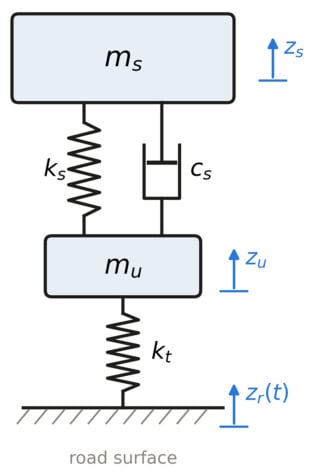
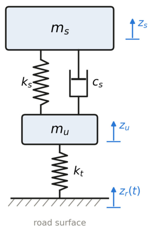
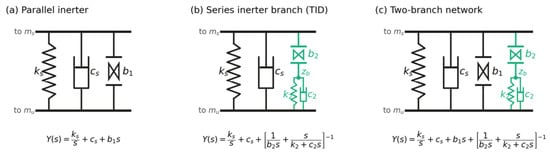
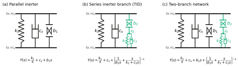
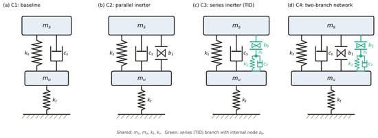
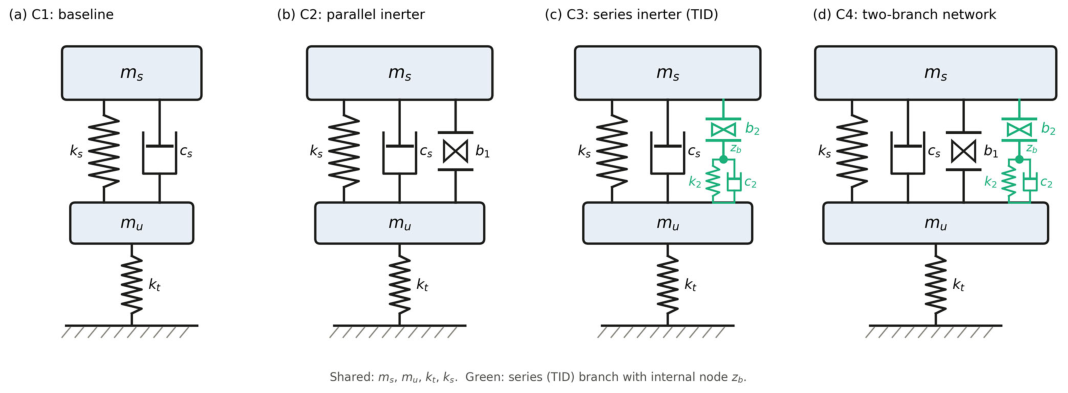
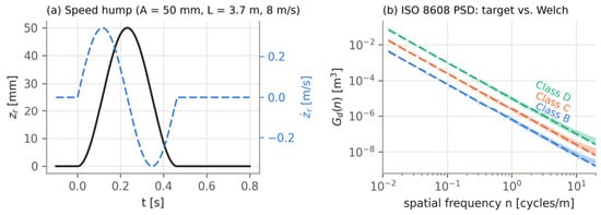
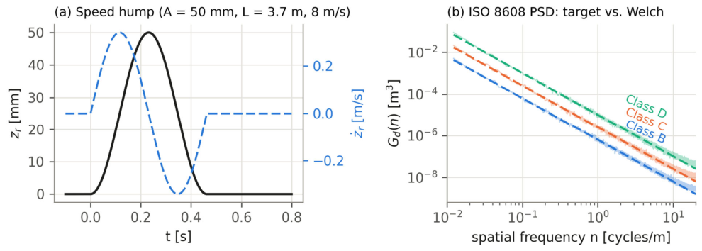
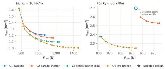
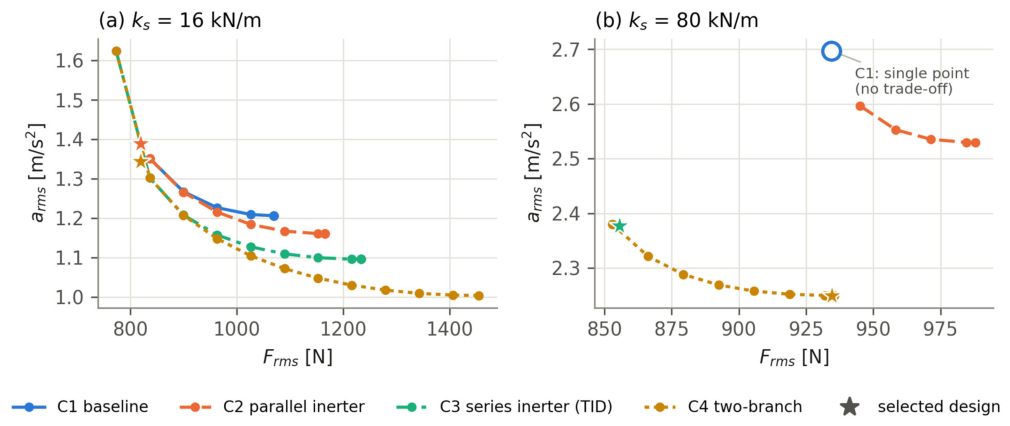
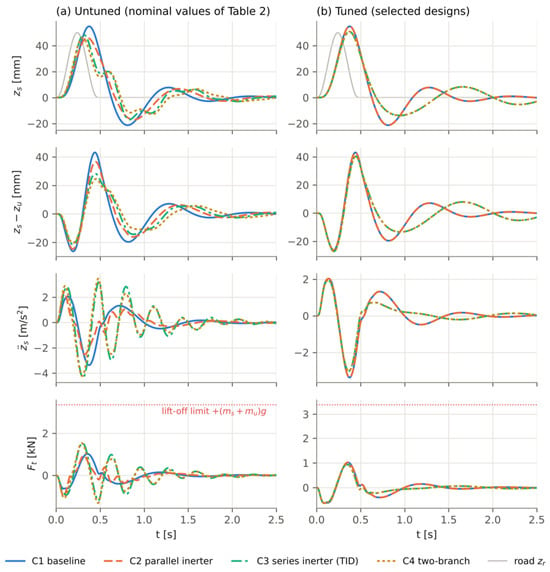
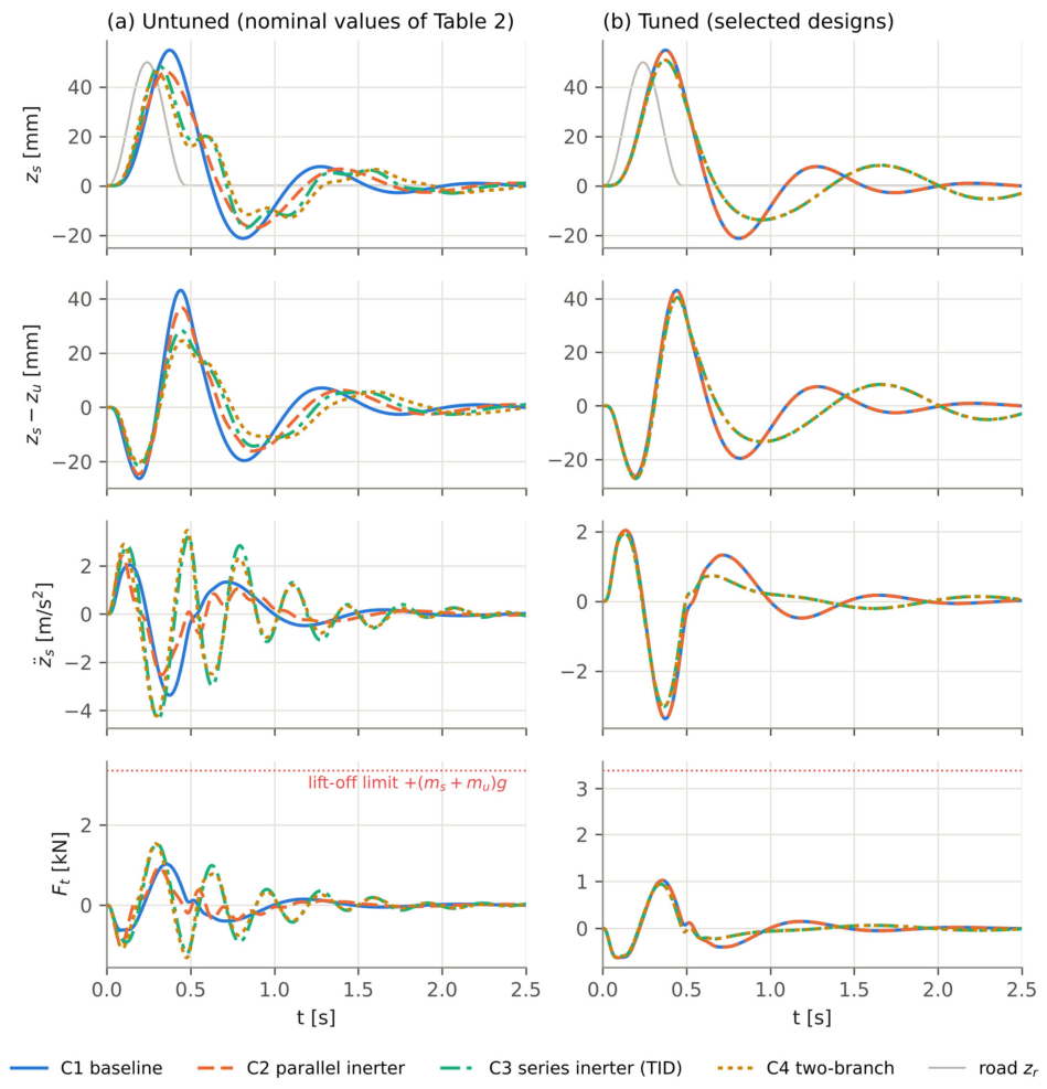
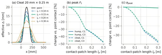
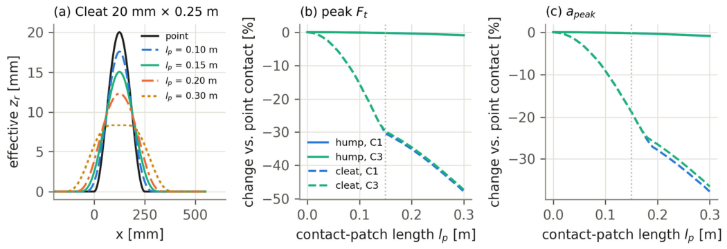
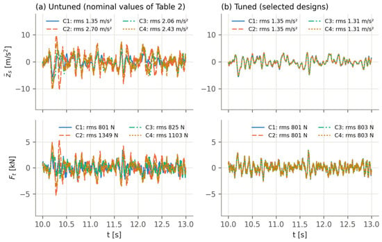
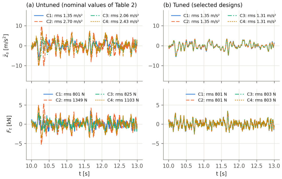
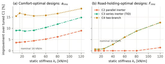
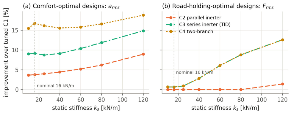
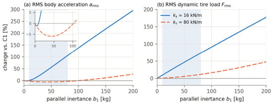
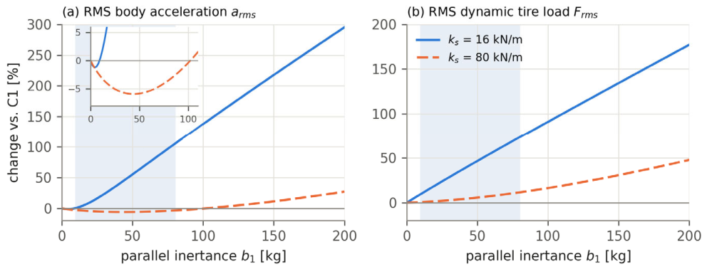

Disclaimer/Publisher’s Note: The statements, opinions and data contained in all publications are solely those of the individual author(s) and contributor(s) and not of MDPI and/or the editor(s). MDPI and/or the editor(s) disclaim responsibility for any injury to people or property resulting from any ideas, methods, instructions or products referred to in the content. |
© 2026 by the authors. Licensee MDPI, Basel, Switzerland. This article is an open access article distributed under the terms and conditions of the Creative Commons Attribution (CC BY) license.