Sampling-Aware Capacity-Feedback Control for Safety-Margin Recovery in Bimanual Robot Grasp-and-Cut Tasks

Abstract

In bimanual grasp-and-cut tasks, the safety distance between arms must be temporarily reduced for close-proximity manipulation and restored after task completion. However, fixed recovery rates or rapid changes in the safety distance can make the recovery infeasible under joint, collision, grasp, and command constraints. To address this issue, we propose a capacity-feedback control framework that adjusts safety-margin recovery according to the robot’s currently feasible control inputs. At each control cycle, a linear program (LP) computes the maximum safety-distance recovery rate supported by the admissible input set. The requested recovery rate is then determined from this capacity with a capacity-scaling factor selected using a sampling-aware tuning rule to reduce the sensitivity of the recovery response to the control period. A subsequent motion-control QP computes the joint-velocity command while satisfying the selected recovery demand and task constraints. Numerical simulations evaluate the recovery behavior and point-wise feasibility of the proposed method under several constraint conditions and compare it with alternative recovery strategies, including fixed-rate recovery. The capacity-feedback behavior is further evaluated in closed-loop rigid-body simulations using Isaac Sim. Sampling-aware tuning reduced the maximum relative recovery-time deviation from 296.634% to 7.143%, while the proposed method successfully completed all 20 physical-robot recovery trials across four task configurations.

1. Introduction

Bimanual manipulation tasks such as grasping, cutting, dissection, and separation often require both robotic arms to operate within a shared, highly constrained workspace. While a safety-distance setpoint is typically imposed to prevent collisions between the arms, it may need to be temporarily reduced during close-proximity operations, such as maintaining a grasp or guiding a cutting tool. Once the close-proximity operation is completed, the reduced setpoint should be restored to its nominal value to obtain sufficient collision clearance between the arms. The challenge is not only to vary the safety-distance setpoint according to the task phase but also to recover it without violating the robot’s motion and task constraints.

However, restoring a reduced safety distance is not simply a matter of increasing the safety-distance setpoint at a fixed rate. As the setpoint increases, the collision-avoidance conditions become more restrictive, while the robot must also satisfy joint-motion limits, grasp constraints, and task requirements. Moreover, because the robot configuration and motion state evolve during the task, a recovery rate that is feasible at one instant may not remain feasible later. Therefore, the recovery rate needs to be adjusted according to the robot’s current motion constraints.

Control Barrier Functions (CBFs) provide a systematic method for satisfying state and safety constraints while minimizing deviations from nominal control inputs [1,2]. However, in the presence of input constraints and multiple simultaneous barrier constraints, the feasibility of the Quadratic Program (QP) is not guaranteed at every control instant. Previous research has addressed this issue through methods such as adaptive CBFs, rate-tunable and optimal-decay formulations, compatibility analysis for multiple CBFs, backup safety sets, and feasible-space monitoring [3,4,5,6,7,8,9]. Recently, Sah and Keshavan derived an exact point-wise feasibility certificate for multi-robot CBF safety filters [10].

Time-varying safety sets and explicit safety recovery have also been studied in the CBF literature. Time-varying CBFs represent constraints whose boundaries evolve with time [11], while dynamic safety margins and prescribed- or exact-time recovery methods regulate how a relaxed safety set returns to a target set [12,13,14]. Related ideas also appear in reference and command governors, which modify a reference so that the closed-loop system remains compatible with constraints [15,16]. Barrier-based governor formulations further extend this concept to constrained output tracking and recursive-feasibility settings [17,18].

CBFs have also been widely applied to the collision avoidance of manipulators and multi-robot systems [19,20]. Recent studies have considered multi-arm interaction using three-dimensional convex geometry, whole-body safety constraints, and full-body safety functions [21,22,23]. Kouidri et al. [24]  investigated external-torque prediction for industrial robot safety.

In practical implementations, CBF constraints are evaluated and applied in the discrete-time domain. Discrete-time and sampled-data CBF formulations analyze safety under finite sampling and zero-order hold [25,26,27,28]. The sampling period and zero-order hold are important factors in the safety analysis of sampled CBF controllers.

Although existing studies provide useful tools for constraint-aware safety control, their primary objectives differ from the recovery problem considered here. Adaptive and optimal-decay CBF methods adjust barrier parameters to improve feasibility [3,4,5], while feasibility analysis methods examine the compatibility of multiple safety constraints [6,7,8,9,10]. Time-varying CBF and safety recovery methods address evolving safety requirements [11,12,13,14], whereas reference governors modify reference commands to satisfy system constraints [15,16,17,18]. However, these approaches do not directly address the online selection of a feasible recovery rate for a task-dependent inter-arm safety-distance setpoint under simultaneous joint, collision, grasp, and command-rate constraints. In particular, a recovery rate that is feasible at RETREAT entry may become infeasible as the robot configuration and admissible input set evolve. To address this problem, the proposed framework computes the maximum point-wise feasible recovery rate at each control cycle and uses it to determine the recovery demand. A sampling-aware tuning rule is further introduced to reduce sensitivity to the control period.

To address these issues, we propose a capacity-feedback control framework for safety-margin recovery in bimanual manipulation. At each control cycle, a Linear Program (LP) computes the maximum safety-distance recovery rate supported by the current admissible input set. This capacity is then used to determine the requested recovery rate, after which the motion-control QP computes the joint-velocity command that satisfies the recovery demand and task constraints. A sampling-aware tuning rule is also introduced to reduce the sensitivity of the recovery response to the control period. The proposed method is evaluated through numerical simulations under different constraint conditions, comparisons with alternative recovery strategies, and closed-loop rigid-body simulations in Isaac Sim together with physical-robot experiments.

Key contributions are summarized as follows:

• A capacity-feedback control framework is proposed to recover a reduced inter-arm safety-distance setpoint after close-proximity bimanual manipulation. At each control cycle, the controller computes the maximum recovery rate allowed by the current admissible input set and uses it as the feasibility capacity.
• The limitation of entry-certified fixed-rate recovery is investigated under the same initial state and constraints. A recovery rate may become infeasible later as the admissible input set changes during the recovery process.
• A sampling-aware tuning rule is introduced to reduce the dependence of the capacity-feedback response on the control period.
• The proposed method is compared with step, time-linear, entry-certified, and direct-rate recovery strategies under representative constraint conditions. Closed-loop rigid-body simulations in Isaac Sim are further used to evaluate the capacity-feedback behavior.

2. Bimanual Task and Safety-Constrained Formulation

2.1. Bimanual Grasp-and-Cut Task

A fixed-base 14-DoF bimanual manipulator is considered,

$$\mathbf{q}={\left[\begin{array}{cc}{\mathbf{q}}_L^{\top }& {\mathbf{q}}_R^{\top }\end{array}\right]}^{\top }\in {\mathbb{R}}^{14},\mathbf{u}=\dot{\mathbf{q}},$$

(1)

where ${\mathbf{q}}_L,{\mathbf{q}}_R\in {\mathbb{R}}^7$ denote the joint-position vectors of the left and right arms, respectively, and $\mathbf{u}$ is the joint-velocity control input.

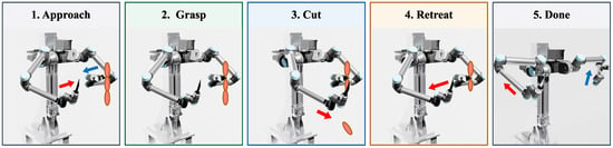
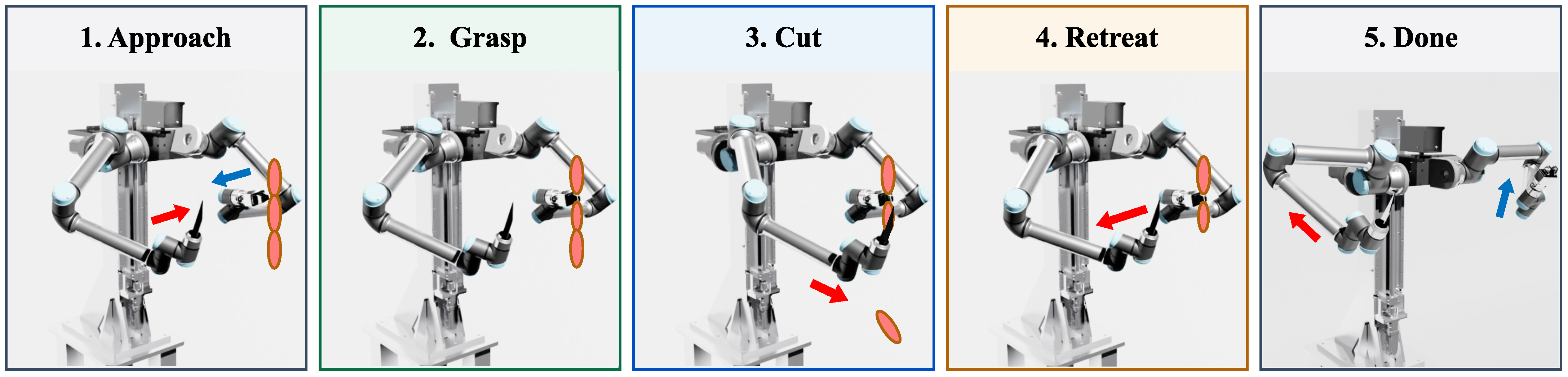
The task sequence illustrated in Figure 1 consists of five phases:

$$\mathrm{APPROACH}\to \mathrm{GRASP}\to \mathrm{CUT}\to \mathrm{RETREAT}\to \mathrm{DONE}.$$

Figure 1. Task sequence for the bimanual grasp-and-cut task. Red arrows indicate the movement direction of the right arm performing the cutting operation, while blue arrows indicate the movement direction of the left arm performing the grasping operation.

During APPROACH, both arms move toward the designated task region. In GRASP, the left arm grasps the workpiece and establishes its reference position. During CUT, the left arm maintains the grasp while the right arm performs the prescribed cutting motion. The inter-arm safety-distance setpoint is reduced to  $r_c$  and held constant  $(\nu =\dot{r}=0)$  to allow close-proximity manipulation.

After CUT, the task enters RETREAT, where the proposed capacity-feedback controller adjusts the recovery rate to restore the safety-distance setpoint toward its nominal value  $r_n$  while satisfying the control constraints. DONE indicates completion of the retreat and safety-margin recovery. Here,  r  denotes the safety-distance setpoint rather than the actual inter-arm distance.

The links and tools are approximated by capsule geometries. The current implementation evaluates 49 cross-arm capsule pairs. For pair i, let $D_i\left(\mathbf{q}\right)$ denote the surface distance and define its distance Jacobian as

$${\mathbf{a}}_i\left(\mathbf{q}\right)={\nabla }_{\mathbf{q}}{D}_i\left(\mathbf{q}\right),{\dot{D}}_i={\mathbf{a}}_i^{\top }\mathbf{u}.$$

(2)

The line-segment distance is computed using the geometric method in [29]. The analytical model focuses on inter-arm safety-margin recovery and does not include same-arm self-collision, environment collision, or task-object mechanics.

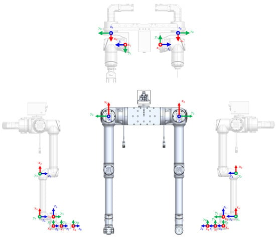
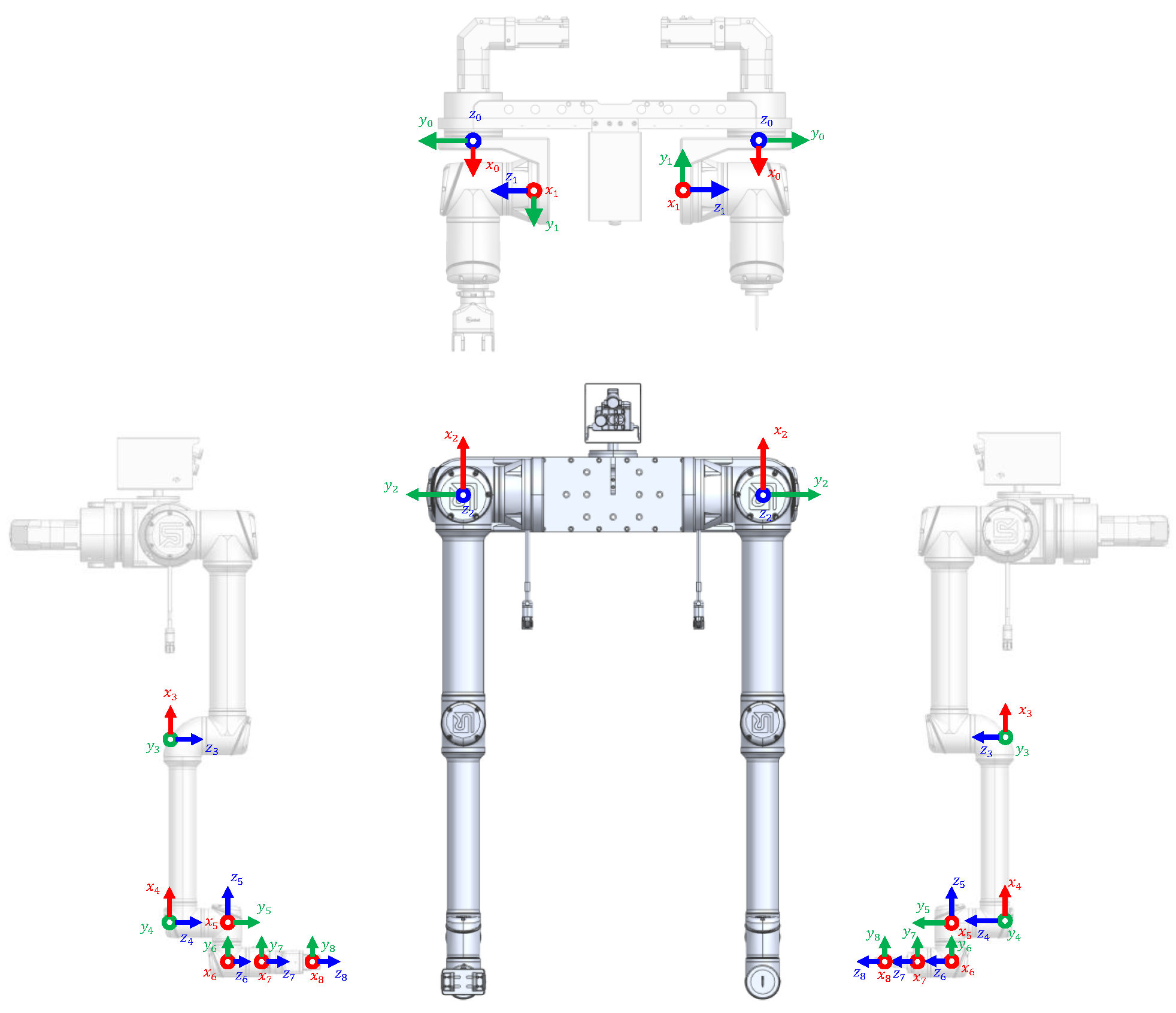
Figure 2 illustrates the kinematic configuration and coordinate frames of the bimanual robotic system. Each arm comprises a six-axis UR manipulator and an additional rotary axis, resulting in seven actuated degrees of freedom per arm. The base coordinate frame, the seven joint coordinate frames of each arm, and the corresponding TCP frames are indicated. The joint indices correspond to the components of ${\mathbf{q}}_L$ and ${\mathbf{q}}_R$ in Equation (1). These coordinate-frame definitions provide the kinematic reference for calculating the task Jacobians and inter-arm collision-distance gradients used in the control formulation.

Figure 2. Kinematic configuration and joint coordinate frames of the 14-DoF bimanual robot. The base, joint, and TCP coordinate frames are indicated for both arms.

2.2. Safety-Constrained Control Formulation

For collision pair i, define the safety function

$$h_i(\mathbf{q},r)=D_i\left(\mathbf{q}\right)-r.$$

(3)

With the safety-distance recovery rate $\nu =\dot{r}$,

$${\dot{h}}_i={\mathbf{a}}_i^{\top }\mathbf{u}-\nu .$$

(4)

Using the exponential CBF condition ${\dot{h}}_i+\beta h_i\ge 0$, where $\beta >0$ is the CBF gain, yields

$${\mathbf{a}}_i^{\top }\mathbf{u}+\beta h_i\ge \nu .$$

(5)

Equation (5) shows how the recovery rate $\nu$ enters the inter-arm collision constraints. In particular, the same recovery rate $\nu$ appears on the right-hand side of all inter-arm collision constraints. Increasing r makes all inter-arm collision constraints more restrictive. Therefore, the recovery rate must be selected according to the current joint, collision, grasp, and command-rate constraints.

A separate minimum-distance constraint is imposed independently of the adaptive setpoint. Let $d_0$ denote the fixed minimum inter-arm distance and ${\beta }_0>0$ the corresponding CBF gain. The constraint is given by

$${\mathbf{a}}_i^{\top }\mathbf{u}+{\beta }_0(D_i-d_0)\ge 0,\forall i.$$

(6)

Thus, reducing the task-dependent setpoint r does not remove the fixed minimum inter-arm distance $d_0$.

Let ${\mathbf{p}}_k={\mathbf{u}}_{k-1}^{\mathrm{cmd}}$ denote the previously issued joint-velocity command. Then, the lower and upper bounds used at control cycle k are

$$\begin{array}{cc}\hfill {\ell }_k& =\max \left\{-v_{\max },-k_q({\mathbf{q}}_k-{\mathbf{q}}_{\min }),{\displaystyle \frac{{\mathbf{q}}_{\min }-{\mathbf{q}}_k}{T_s}},{\mathbf{p}}_k-T_s\overline{a}\right\},\hfill \\ \hfill {\mathbf{h}}_k^u& =\min \left\{v_{\max },k_q({\mathbf{q}}_{\max }-{\mathbf{q}}_k),{\displaystyle \frac{{\mathbf{q}}_{\max }-{\mathbf{q}}_k}{T_s}},{\mathbf{p}}_k+T_s\overline{a}\right\},\hfill \end{array}$$

(7)

where ${\mathbf{q}}_k$ denotes the joint-position vector at control cycle k, ${\mathbf{q}}_{\min }$ and ${\mathbf{q}}_{\max }$ are the joint-position limits, $v_{\max }$ is the joint-velocity limit, $k_q>0$ is the joint-limit approach gain, $T_s$ is the control period, and $\overline{a}$ is the command-rate limit. The four terms represent, respectively, joint-velocity limits, joint-limit approach bounds, one-step position consistency, and command-rate limits. The command-rate terms are particularly important for the recovery problem because the current admissible box depends explicitly on the previous command ${\mathbf{p}}_k$ and on the control period $T_s$.

The one-step joint-position bounds follow from the discrete kinematic update ${\mathbf{q}}_{k+1}={\mathbf{q}}_k+T_s{\mathbf{u}}_k$, while the command-rate bounds are obtained from  $|{\mathbf{u}}_k-{\mathbf{p}}_k|\le T_s\overline{a}$, which is applied component-wise. Equation  (7)  combines these bounds with the joint-velocity limits and joint-limit approach constraints through their component-wise intersection.

Define

$${\mathcal{B}}_k=\left\{\mathbf{u}:{\ell }_k\le \mathbf{u}\le {\mathbf{h}}_k^u\right\}.$$

(8)

Let ${\mathcal{G}}_k$ denote the phase-dependent grasp-constraint set defined in Section 2.3. The admissible control set is

$${\mathcal{U}}_k=\left\{\mathbf{u}\in {\mathcal{B}}_k:{\mathbf{a}}_i^{\top }\mathbf{u}+{\beta }_0(D_i-d_0)\ge 0,\mathbf{u}\in {\mathcal{G}}_k\right\}.$$

(9)

The recovery demand $\nu$ is not included in ${\mathcal{U}}_k$ and enters separately through (5). This separation allows the feasible recovery rate to be evaluated over the current admissible input set.

2.3. Grasp Constraint During Recovery

During CUT and LOCK-mode RETREAT, the left arm maintains the grasp, and the left TCP is kept near its grasp reference. Let

$${\mathbf{e}}_L={\mathbf{x}}_L-{\mathbf{x}}_{L,0}$$

denote the left-TCP position error, where ${\mathbf{x}}_L$ and ${\mathbf{x}}_{L,0}$ are the current and reference positions, respectively. The desired corrective TCP velocity is $-K_e{\mathbf{e}}_L$, where $K_e>0$ is the grasp-position feedback gain.

Since the desired corrective velocity may not be compatible with the joint-velocity bounds, a joint-velocity target is obtained by

$${\mathbf{u}}^{\mathrm{gr}}\in \arg \underset{\mathbf{v}\in {\mathcal{B}}_k}{\min }{∥\mathbf{B}\mathbf{v}+K_e{\mathbf{e}}_L∥}_2^2,$$

(10)

where $\mathbf{v}\in {\mathbb{R}}^{14}$ is a candidate joint-velocity vector and $\mathbf{B}\in {\mathbb{R}}^{3\times 14}$ is the left-TCP position Jacobian. The resulting TCP velocity is used to define the grasp-constraint set as

$${\mathcal{G}}_k=\left\{\mathbf{u}\in {\mathbb{R}}^{14}:\mathbf{B}\mathbf{u}=\mathbf{B}{\mathbf{u}}^{\mathrm{gr}}\right\}$$

(11)

during CUT and LOCK-mode RETREAT. When the grasp constraint is inactive, ${\mathcal{G}}_k={\mathbb{R}}^{14}$.

The projection in (10) considers only the joint-velocity bounds in ${\mathcal{B}}_k$. The resulting grasp constraint is included in the admissible set ${\mathcal{U}}_k$ together with the minimum-distance constraint.

During RETREAT, the controller selects the recovery rate ${\nu }_k$ and the joint-velocity command ${\mathbf{u}}_k$ such that ${\mathbf{u}}_k\in {\mathcal{U}}_k$ and the inter-arm CBF constraints in (5) are satisfied while $r_k$ is restored toward $r_n$. Because the admissible set ${\mathcal{U}}_k$ changes during the recovery process, a recovery rate that is feasible at one control instant may become infeasible later.

3. Feasibility Capacity Analysis for Safety-Margin Recovery

3.1. Feasibility Capacity and Setpoint Dependence

For a fixed control cycle, define the maximum recovery rate supported by the current admissible set as

$${\kappa }_k\left(r\right)=\underset{\mathbf{u}\in {\mathcal{U}}_k}{\max }\underset{i}{\min }\left[{\mathbf{a}}_i^{\top }\mathbf{u}+\beta (D_i-r)\right].$$

(12)

For a given admissible command  $\mathbf{u}$, each term in Equation  (12) represents the upper bound on the safety-distance recovery rate imposed by the corresponding collision constraint. The inner minimum therefore determines the maximum common recovery rate supported by that command, while maximization over  ${\mathcal{U}}_k$ yields the largest feasible rate  ${\kappa }_k$ under the current control constraints. This rate describes the allowable change of the safety-distance setpoint rather than the physical separation velocity of the robot arms. If  ${\kappa }_k$ is negative, no nonnegative recovery rate is feasible at the current control sample.

For a prescribed recovery rate $\nu$, each inter-arm collision constraint defines a half-space in the control-input space. Increasing $\nu$ tightens these constraints, and ${\kappa }_k\left(r\right)$ is the largest recovery rate for which their intersection with ${\mathcal{U}}_k$ remains nonempty.

An equivalent LP is

$$\begin{array}{cc}\hfill \underset{\mathbf{u},\eta }{\max }& \eta \hfill \\ \hfill \mathrm{s}.\mathrm{t}.& \mathbf{u}\in {\mathcal{U}}_k,\hfill \\ \hfill & \eta -{\mathbf{a}}_i^{\top }\mathbf{u}\le \beta (D_i-r),\forall i.\hfill \end{array}$$

(13)

At each control cycle, the robot state, safety-distance setpoint, and constraint coefficients are treated as fixed parameters. Since the admissible input set is defined by affine constraints, Equation  (13)  constitutes a linear program in the decision variables  $\mathbf{u}$  and  $\eta$ with a linear objective and affine constraints. If the admissible input set  ${\mathcal{U}}_k$  is nonempty and compact, the LP admits a finite optimal solution.

The optimal value is denoted by ${\kappa }_k={\eta }^{★}$. The LP solution identifies the maximum feasible recovery rate but is not used directly as the robot command. The motion-control QP determines the actual joint-velocity command according to the task objectives while satisfying the imposed constraints.

For fixed ${\mathbf{q}}_k$, ${\mathbf{p}}_k$, ${\mathcal{U}}_k$, distance Jacobians, and gain $\beta$, changing only the setpoint from r to $r^{\prime }$ shifts every inter-arm collision constraint by the same scalar amount. Consequently,

$${\kappa }_k\left(r^{\prime }\right)={\kappa }_k\left(r\right)-\beta (r^{\prime }-r).$$

(14)

This relation follows directly because replacing r by $r^{\prime }$ subtracts the same quantity $\beta (r^{\prime }-r)$ from every term inside the minimum in (12). Thus, at a fixed robot state and admissible set, increasing the required margin by $\Delta r$ reduces the available recovery capacity by $\beta \Delta r$. The relation is only a fixed-sample identity: once a command is applied, the robot geometry and admissible input set can change, so (14) does not determine ${\kappa }_{k+1}$.

3.2. Point-Wise Feasibility Characterization

The capacity ${\kappa }_k$ gives an exact current-sample feasibility threshold for a prescribed recovery rate. Suppose that ${\mathcal{U}}_k$ is nonempty, the LP in (13) has a finite optimum, and the remaining hard constraints do not depend on the prescribed recovery rate $\nu$. Under these conditions, the fixed-$\nu$ control QP is mathematically feasible at the current sample if and only if

$$\nu \le {\kappa }_k.$$

(15)

To see this, if the fixed-$\nu$ QP is feasible, there exists a command $\mathbf{u}\in {\mathcal{U}}_k$ such that ${\mathbf{a}}_i^{\top }\mathbf{u}+\beta (D_i-r)\ge \nu$ for every i. The inner minimum in (12) is therefore at least $\nu$ for that command, and maximization over ${\mathcal{U}}_k$ gives ${\kappa }_k\ge \nu$. Conversely, when $\nu \le {\kappa }_k$, the optimal LP solution ${\mathbf{u}}^{★}$ satisfies ${\mathbf{a}}_i^{\top }{\mathbf{u}}^{★}+\beta (D_i-r)\ge {\kappa }_k\ge \nu$ for all i. Therefore, ${\mathbf{u}}^{★}$ is a feasible point for the fixed-$\nu$ QP.

A recovery rate selected only at RETREAT entry is not guaranteed to remain feasible throughout recovery. For the entry-certified fixed-rate policy, the recovery rate is determined once from the entry capacity and then held constant. Since the admissible input set changes during recovery, the corresponding capacity can decrease below the fixed recovery rate at a later control instant.

3.3. Capacity Reserve

For any prescribed recovery rate ${\nu }_k$, define the point-wise recovery-capacity reserve as

$${\sigma }_k={\kappa }_k-{\nu }_k.$$

(16)

From the point-wise feasibility condition in (15), ${\sigma }_k\ge 0$ indicates that the requested recovery rate ${\nu }_k$ is feasible at the current control instant. The reserve represents the difference between the maximum feasible recovery rate and the requested rate.

The capacity reserve should not be confused with the minimum CBF residual of the command selected by the motion-control QP. For an accepted command ${\mathbf{u}}_k$, define

$$s_k^{\mathrm{cmd}}=\underset{i}{\min }\left[{\mathbf{a}}_i^{\top }{\mathbf{u}}_k+\beta (D_i-r_k)-{\nu }_k\right].$$

(17)

From the definition of ${\kappa }_k$,

$$s_k^{\mathrm{cmd}}\le {\kappa }_k-{\nu }_k={\sigma }_k.$$

(18)

Therefore, a positive capacity reserve does not imply that the command selected by the QP has the same constraint margin nor does it quantify robustness to actuator or model errors. In exact arithmetic, a mathematically feasible QP command satisfies $s_k^{\mathrm{cmd}}\ge 0$; in numerical implementation, small signed residuals can remain at the solver-tolerance scale.

4. Sampling-Aware Capacity-Feedback Recovery Control

4.1. Capacity-Feedback Recovery Law

The proposed controller recalculates ${\kappa }_k$ at every control cycle and uses it to select the requested safety-distance recovery rate. This policy is referred to as the per-cycle capacity-feedback policy. For valid input bounds and a finite LP optimum, the implemented law is

$${\nu }_k=\left\{\begin{array}{cc}0,\hfill & r_k\ge r_n-{\epsilon }_{\mathrm{stop}},\hfill \\ \min \left\{\overline{\nu },\theta {\kappa }_k,(r_n-r_k)/T_s\right\},\hfill & r_k<r_n-{\epsilon }_{\mathrm{stop}},{\kappa }_k\ge 0,\hfill \\ {\kappa }_k/\theta ,\hfill & r_k<r_n-{\epsilon }_{\mathrm{stop}},{\kappa }_k<0,\hfill \end{array}\right.0<\theta <1$$

(19)

where $\overline{\nu }>0$ is the maximum recovery-rate limit, ${\epsilon }_{\mathrm{stop}}>0$ is the stopping tolerance, and $0<\theta <1$ is the capacity-scaling factor. The first branch stops the setpoint update near the nominal target. When ${\kappa }_k\ge 0$, the requested rate is limited by $\overline{\nu }$, $\theta {\kappa }_k$, and the remaining distance to $r_n$ within one control cycle. When ${\kappa }_k<0$, the controller temporarily relaxes the safety-distance setpoint by selecting a negative recovery rate.

After a numerically accepted QP command, the setpoint is updated by

$$r_{k+1}={clip}_{[d_0,r_n]}\left(r_k+T_s{\nu }_k\right).$$

(20)

Here, ${clip}_{[d_0,r_n]}(·)$ limits the updated setpoint to the interval $[d_0,r_n]$.

For active recovery with ${\kappa }_k\ge 0$,

$${\nu }_k\le \theta {\kappa }_k\le {\kappa }_k,{\kappa }_k-{\nu }_k\ge (1-\theta ){\kappa }_k.$$

(21)

Thus, the requested recovery rate leaves a capacity reserve of at least $(1-\theta ){\kappa }_k$. As discussed in Section 3.3, this reserve characterizes point-wise feasibility and does not guarantee future feasibility or actuator-level robustness.

Under the ideal continuous-time kinematic model, if the CBF conditions are satisfied for all time and the initial safety constraints hold, the comparison principle yields  $h_i\left(t\right)\ge h_i\left(0\right)e^{-\beta t}\ge 0$, ensuring forward invariance of the corresponding safety set. However, this conditional result does not establish closed-loop tracking stability or convergence of the safety-distance setpoint. Furthermore, the proposed controller enforces the constraints at discrete control instants, and actuator tracking errors and model uncertainties may affect their satisfaction between samples. Therefore, point-wise feasibility does not guarantee recursive feasibility or continuous-time safety. The physical-robot experiments in Section 5.6  provide additional empirical validation under the tested operating conditions rather than a general robustness guarantee.

The factor $\theta$ determines how much of the current capacity is requested in the capacity-limited branch. Using the same value of $\theta$ at different control periods can result in different recovery responses, because $T_s$ affects both the command-rate bounds and the controller update rate.

To reduce the dependence on the control period, the factor $1-\theta$ is scaled with $T_s$. The sampling-aware design rule is

$${\displaystyle \frac{1-\theta }{T_s}}=c,$$

(22)

or equivalently

$$\theta =1-c{T}_s,0<c{T}_s<1.$$

(23)

Here, c has units of inverse time and serves as a control-period-normalized tuning parameter. The rule keeps the normalized fractional back-off $(1-\theta )/T_s$ constant when $T_s$ changes. Equations (22) and (23) are used as a sampling-aware tuning rule for the proposed controller.

We chose $c=(1-{\theta }_{\mathrm{ref}})/T_{s,\mathrm{ref}}=5{\mathrm{s}}^{-1}$ from ${\theta }_{\mathrm{ref}}=0.95$ at $T_{s,\mathrm{ref}}=10$ ms rather than by optimization. At this period, the choice leaves 5% of positive capacity as a point-wise rate reserve when capacity limits the request. The effect of changing c is tested in Section 5.3; this reserve is not a geometric safety guarantee.

4.2. Motion-Control QP Under Recovery Constraints

Once ${\nu }_k$ is selected, the proposed controller determines the joint-velocity command from

$$\underset{\mathbf{u}}{\min }{F}_k(\mathbf{u};w_k)\mathrm{s}.\mathrm{t}.\mathbf{u}\in {\mathcal{U}}_k,{\mathbf{a}}_i^{\top }\mathbf{u}+\beta (D_i-r_k)\ge {\nu }_k(\forall i).$$

(24)

For CUT and RETREAT, the objective is

$$F_k(\mathbf{u};w_k)={\displaystyle \frac{1}{2}}\parallel {\mathbf{J}}_R\mathbf{u}-{\mathbf{V}}_R^{\mathrm{cmd}}{\parallel }_{{\mathbf{Q}}_R}^2+{\displaystyle \frac{w_k}{2}}{\parallel \mathbf{B}\mathbf{u}\parallel }_{\mathbf{S}}^2+{\displaystyle \frac{1}{2}}\parallel \mathbf{u}-{\mathbf{u}}_{\mathrm{post}}{\parallel }_{\mathbf{R}}^2+{\displaystyle \frac{{\eta }_u}{2}}{\parallel \mathbf{u}-{\mathbf{p}}_k\parallel }_2^2$$

(25)

where ${\mathbf{J}}_R$ is the right-TCP Jacobian, ${\mathbf{V}}_R^{\mathrm{cmd}}$ is the commanded right-TCP velocity, ${\mathbf{u}}_{\mathrm{post}}$ is the posture command, and ${\mathbf{Q}}_R$, $\mathbf{S}$, $\mathbf{R}$, $w_k$, and ${\eta }_u$ are weighting terms. The terms correspond to right-arm task tracking, left-TCP motion suppression, posture regulation, and command smoothing. During CUT and LOCK-mode RETREAT, the left-TCP velocity is already fixed by the hard grasp equality in Section 2.3; therefore, the second term is constant over the feasible set and does not affect the exact QP optimizer. When the hard grasp equality is inactive, this term penalizes left-TCP motion.

For a fixed recovery rate ${\nu }_k$, Equation (24) defines a quadratic program with joint velocity $\mathbf{u}$ as the decision variable and affine constraints. The objective function is convex when the weighting matrices are positive semidefinite and the scalar weights are nonnegative. In particular, if ${\eta }_u>0$, the command-smoothing term makes the Hessian positive definite, ensuring a unique optimal solution whenever the QP is feasible. Under the assumptions stated in Section 3.2, feasibility is characterized by ${\nu }_k\le {\kappa }_k$.

The capacity LP and the control QP serve different roles. The LP determines how much recovery demand can be supported, while the QP determines the robot motion that satisfies the selected demand and task objectives.

Kinematic singularities may affect the proposed controller by reducing the achievable task-space motion in certain directions. Since the formulation does not require Jacobian inversion, singularities do not inherently make the LP or QP ill-defined. However, reduced task-space mobility may degrade TCP tracking, while the feasibility capacity depends on the current robot configuration and admissible control constraints. The proposed controller does not explicitly guarantee singularity avoidance, which remains a limitation of this study.

4.3. Direct-Rate QP Baseline

For comparison, the direct-rate baseline jointly optimizes the joint-velocity command $\mathbf{u}$ and recovery rate $\nu$ within a single QP,

$$\begin{array}{cc}\hfill \underset{\mathbf{u},\nu }{\min }& F_k(\mathbf{u};w_k)+{\displaystyle \frac{{\lambda }_{\nu }}{2}}{(\nu -{\nu }_{\mathrm{ref}})}^2\hfill \\ \hfill \mathrm{s}.\mathrm{t}.& \mathbf{u}\in {\mathcal{U}}_k,\hfill \\ \hfill & {\mathbf{a}}_i^{\top }\mathbf{u}+\beta (D_i-r_k)\ge \nu ,\forall i,\hfill \\ \hfill & k_{\mathrm{req}}(r_n-r_k)\le \nu \le \min \left\{\overline{\nu },{\displaystyle \frac{r_n-r_k}{T_s}}\right\}.\hfill \end{array}$$

(26)

where ${\lambda }_{\nu }>0$ is the recovery-rate weighting factor, ${\nu }_{\mathrm{ref}}$ is the reference recovery rate, and $k_{\mathrm{req}}>0$ defines the minimum recovery-rate requirement.

The direct-rate baseline uses the same admissible set and motion objective, but the rate-selection trade-off is embedded directly in the QP through ${\lambda }_{\nu }$ and ${\nu }_{\mathrm{ref}}$. This baseline is used to compare the proposed LP–QP separation with a direct co-optimization of motion and recovery rate.

4.4. Overall Control Architecture

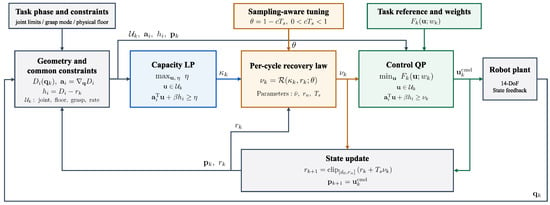
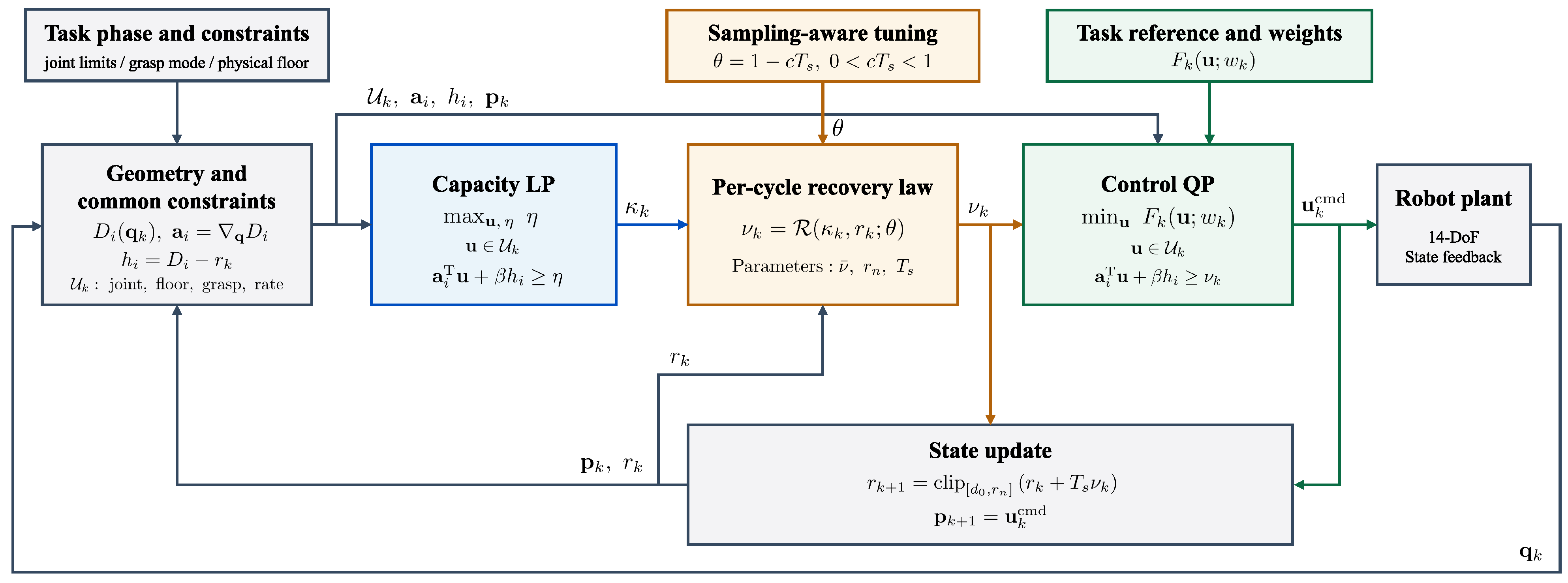
Figure 3 summarizes the overall control architecture. At each control cycle, the current joint state ${\mathbf{q}}_k$, previous command ${\mathbf{p}}_k$, and safety-distance setpoint $r_k$ are used to construct the admissible input set ${\mathcal{U}}_k$. The capacity LP computes ${\kappa }_k$, which determines the requested recovery rate ${\nu }_k$. The motion-control QP then generates the joint-velocity command  ${\mathbf{u}}_k^{\mathrm{cmd}}$ satisfying the recovery and task constraints. After numerical acceptance, the command is applied and retained for the next cycle, and the setpoint is updated.

Figure 3. Overall capacity-feedback control architecture.

The control steps during RETREAT are given in Algorithm 1.

Algorithm 1 Capacity-feedback recovery during RETREAT

Input: Current state ${\mathbf{q}}_k$, previous command ${\mathbf{p}}_k$, and setpoint $r_k$. 1.  Compute inter-arm distances $D_i$, gradients ${\mathbf{a}}_i$, task Jacobians, and active grasp constraints. 2.  Construct the admissible set ${\mathcal{U}}_k$ from the joint, command-rate, minimum-distance, and grasp constraints. 3.  Solve the capacity LP (13) to obtain ${\kappa }_k$.    if the LP fails, terminate without updating the state or setpoint. 4.  Use $\theta =1-c{T}_s$ when sampling-aware tuning is enabled, and select ${\nu }_k$ by (19). 5.  Solve the control QP (24) for ${\mathbf{u}}_k^{\mathrm{cmd}}$.    if the QP fails, terminate without updating the state or setpoint. 6.  Apply ${\mathbf{u}}_k^{\mathrm{cmd}}$, set ${\mathbf{p}}_{k+1}={\mathbf{u}}_k^{\mathrm{cmd}}$, and update $r_{k+1}$ using (20).

5. Simulation Results and Physics-Based Validation

5.1. Simulation Setup and Evaluation Metrics

The Python(version 3.13.3) evaluation used the 14-DoF bimanual model and 49 cross-arm capsule pairs described in Section 2. Unless otherwise specified, the common parameters were $T_s=10$ ms, $d_0=0.02$ m, $r_c=0.05$ m, $r_n=0.12$ m, $\beta =4{\mathrm{s}}^{-1}$, ${\beta }_0=8{\mathrm{s}}^{-1}$, and $\theta =0.95$. The recovery-rate cap, joint-velocity and acceleration limits, and QP initialization were set separately for each study. HiGHS solved the capacity LP [30], and OSQP solved the control QP [31]. The model updates the commanded joint state at the velocity level. It was used for controlled numerical evaluation rather than as a rigid-body dynamics simulator.

The distance values define the simulated task rather than hardware-calibrated safety limits: $d_0$ is the fixed minimum distance, $r_c$ is the CUT setpoint, and $r_n$ is the RETREAT target. The gain $\beta$ acts on the changing setpoint, while ${\beta }_0$ acts on the fixed minimum-distance constraint. Both gains were held fixed in the policy comparisons. The relation between $\theta$ and c is given in Section 4.1, and their sensitivity is examined in Section 5.3.

Recovery time $T_{\mathrm{rec}}$ was defined as the start of the first 0.2 s confirmation interval over which both $r_k\ge r_n-0.005$ m and $D_{\min ,k}\ge r_k-0.005$ m held. Solver failures were recorded as failures rather than counted as successful recoveries.

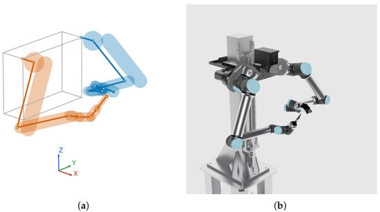
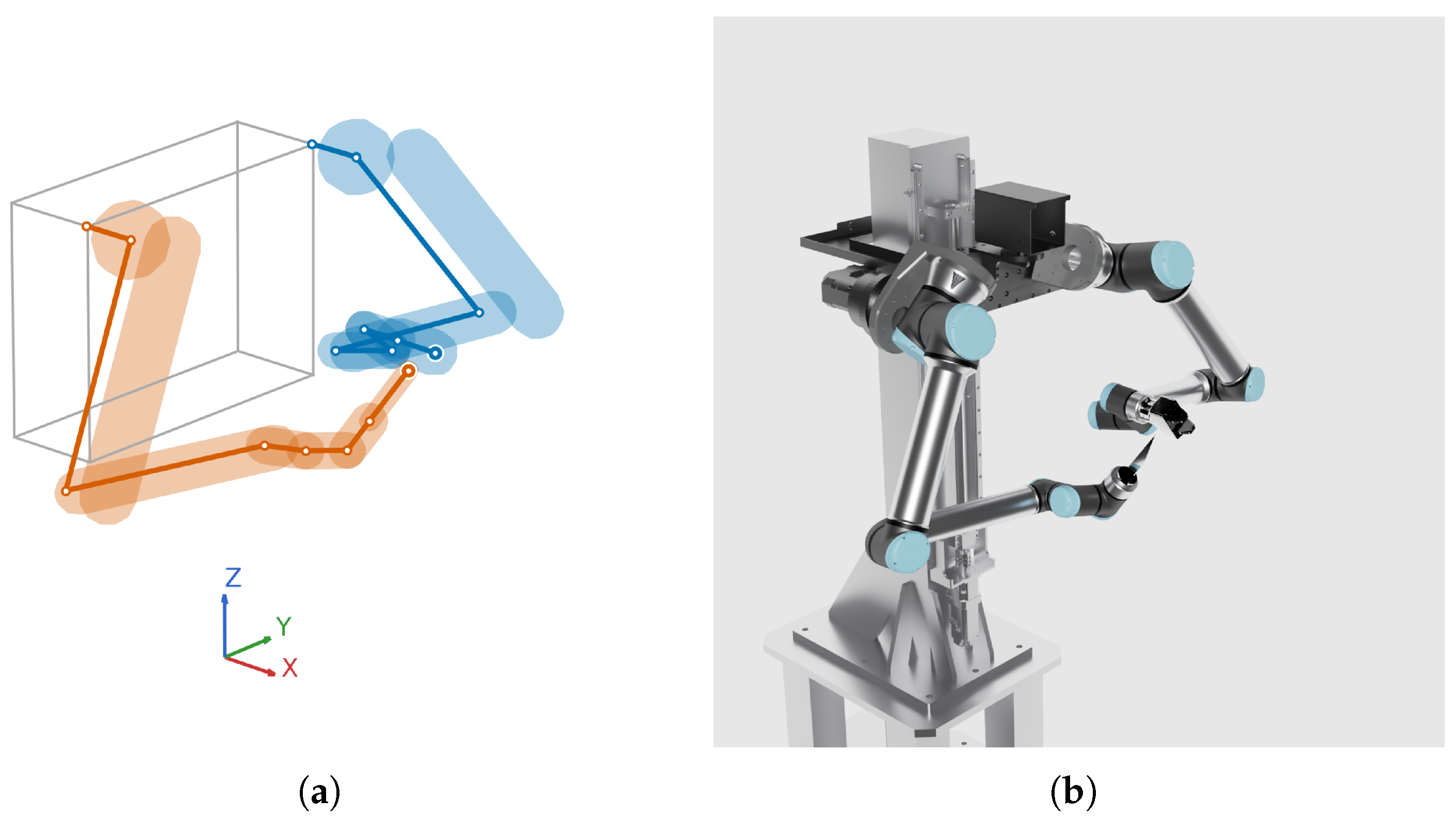
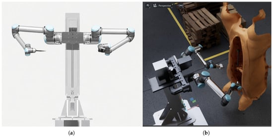
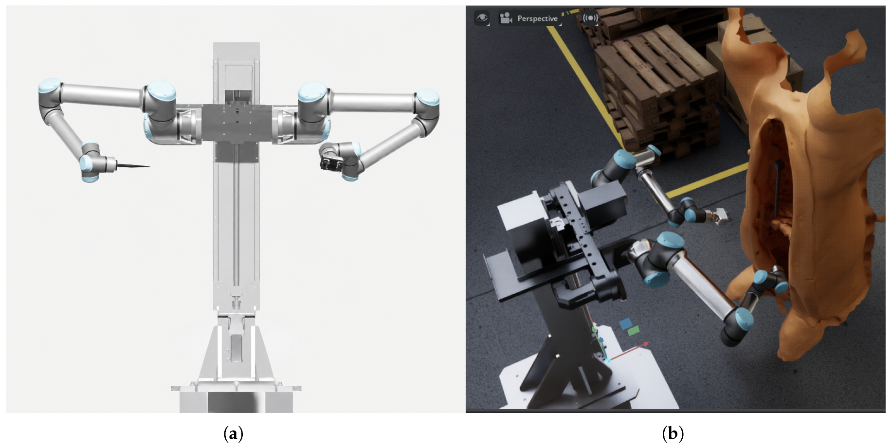
Figure 4 shows the Python-based kinematic model with capsule collision geometry and the corresponding robot configuration in Isaac Sim.

Figure 4. Simulation environments. (a) Python-based bimanual kinematic model with capsule collision geometry. (b) Corresponding bimanual robot configuration in NVIDIA Isaac Sim.

5.2. Point-Wise Feasibility Capacity and Closed-Loop Recovery

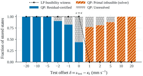
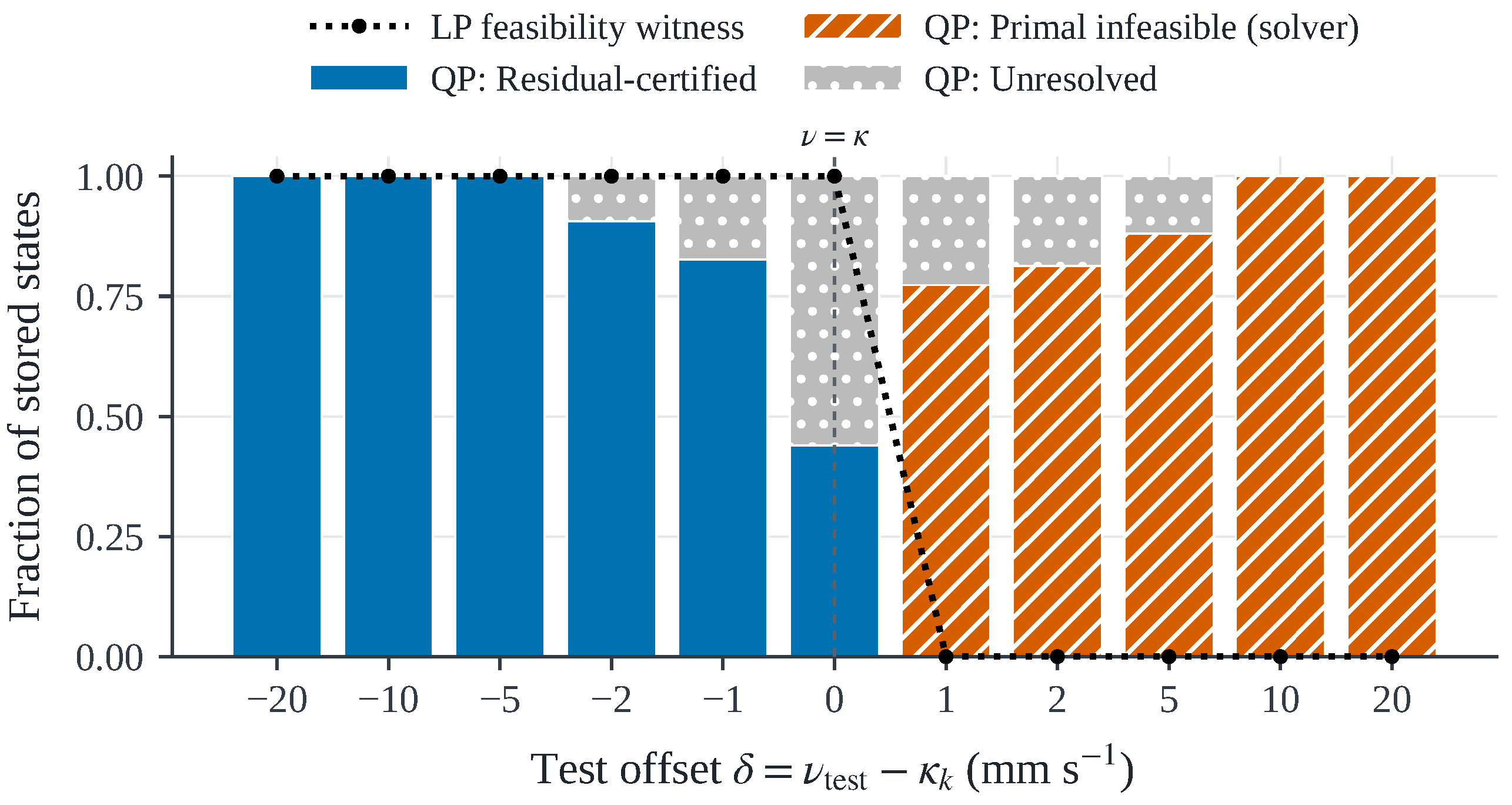
The point-wise interpretation of ${\kappa }_k$ was first tested at 75 RETREAT states stored from three successful trajectories. Each state was evaluated without propagation. For each stored condition, the robot state, previous command, safety-distance setpoint, and common admissible constraints were held fixed while ${\nu }_{\mathrm{test}}={\kappa }_k+\delta$ was evaluated at 11 offsets from $-0.02$ to $+0.02$ m/s. Figure 5 summarizes the stored-state feasibility results near $\nu =\kappa$.

Figure 5. Point-wise feasibility validation near $\nu =\kappa$ using stored RETREAT states.

For $\delta \le 0$, an LP feasibility witness existed at all 75 stored states. For $\delta \ge 0.001$ m/s, none of the states admitted a witness. Some QP solves did not converge close to the boundary; these numerical failures were kept separate from mathematical infeasibility. Bisection resolved the QP boundary at 33 stored states. Across those states, the mean and maximum values of $|{\nu }_{\mathrm{QP},\max }-{\kappa }_k|$ were $8.62\times {10}^{-7}$ and $1.77\times {10}^{-6}$ m/s, respectively.

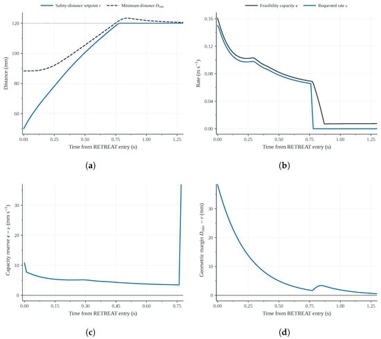
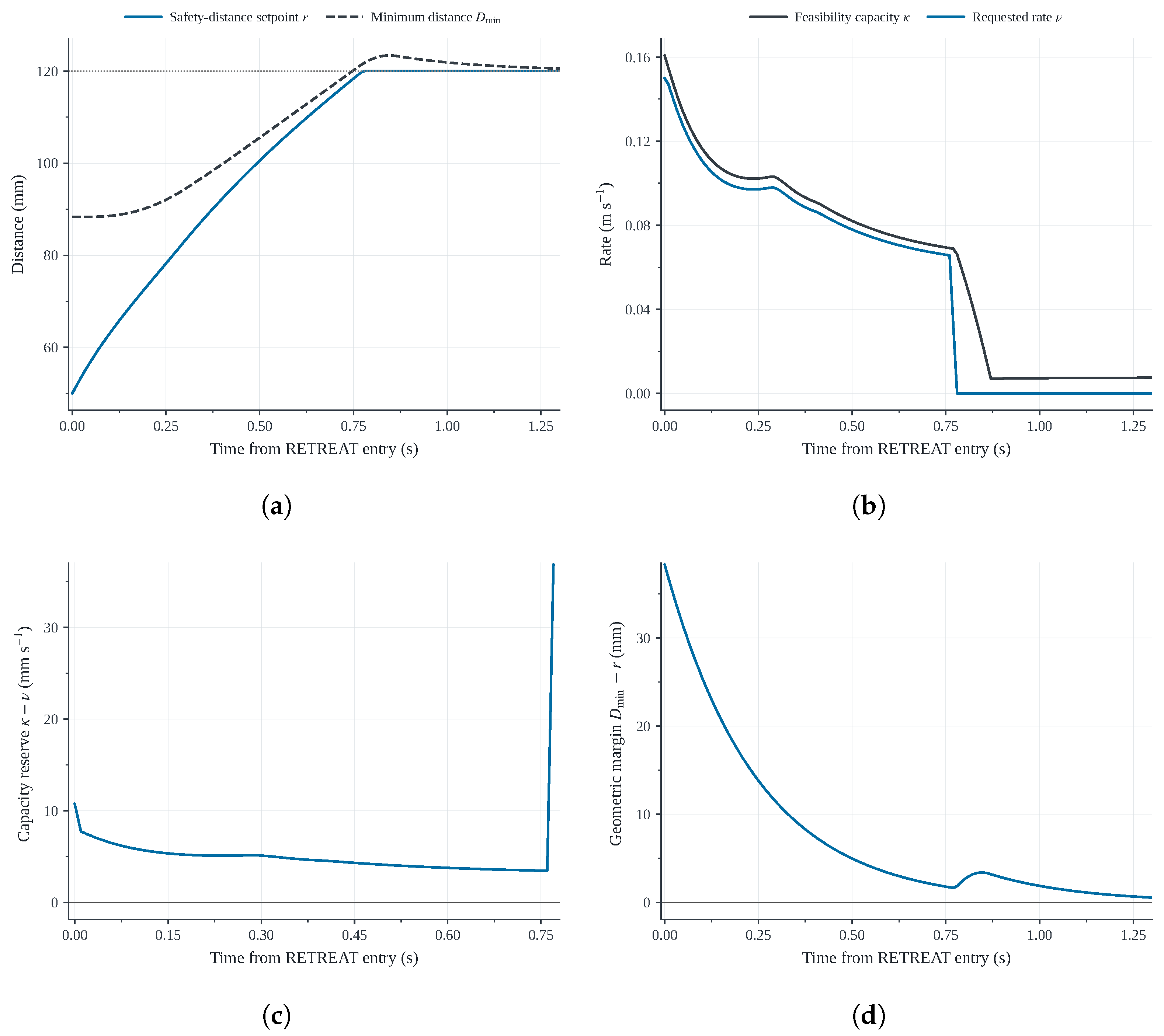
The same mechanism was then examined along a closed-loop RETREAT trajectory. In a representative capacity-limited condition, ${\kappa }_{\mathrm{entry}}=0.160767$ m/s and $\overline{\nu }=0.15$ m/s. The proposed controller recomputed ${\kappa }_k$ at every sample and restored the setpoint from 50 to 120 mm in 0.70 s. The minimum capacity reserve during active recovery was 0.003456 m/s. Figure 6 shows the corresponding closed-loop recovery response of the proposed policy. The requested recovery rate is adjusted according to the changing feasibility capacity, maintaining a positive capacity reserve during active recovery.

Figure 6. Safety-margin recovery with the proposed capacity-feedback policy. (a) Safety-distance setpoint and minimum distance. (b) Feasibility capacity and requested rate. (c) Capacity reserve. (d) Geometric safety margin

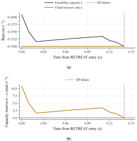
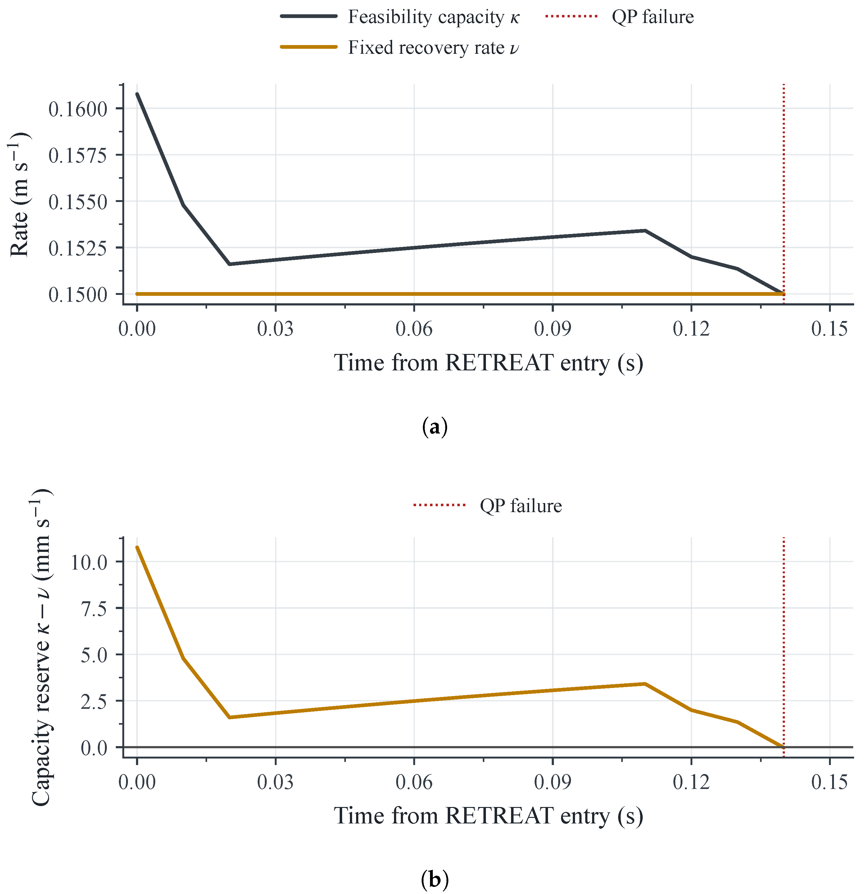
The entry-certified policy, by contrast, kept its initially feasible request fixed. About 0.14 s after RETREAT entry, the evolving capacity fell below the fixed request, and the control QP became primal infeasible. Figure 7 shows the corresponding loss of point-wise feasibility.

Figure 7. Loss of point-wise feasibility under the entry-certified fixed-rate policy. (a) Capacity and fixed recovery rate. (b) Capacity reserve.

Equation (14) alone predicts a crossing at approximately 0.02 s if r is the only quantity that changes from its entry value. The crossing in the closed-loop trajectory occurred at 0.14 s. Along the closed-loop trajectory, the capacity changes with the robot state, geometry, previous command, and admissible input set. Thus, ${\kappa }_{\mathrm{entry}}$ certifies feasibility at a point; it does not guarantee feasibility over the full trajectory.

5.3. Control-Period Sensitivity and Sampling-Aware Tuning

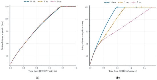
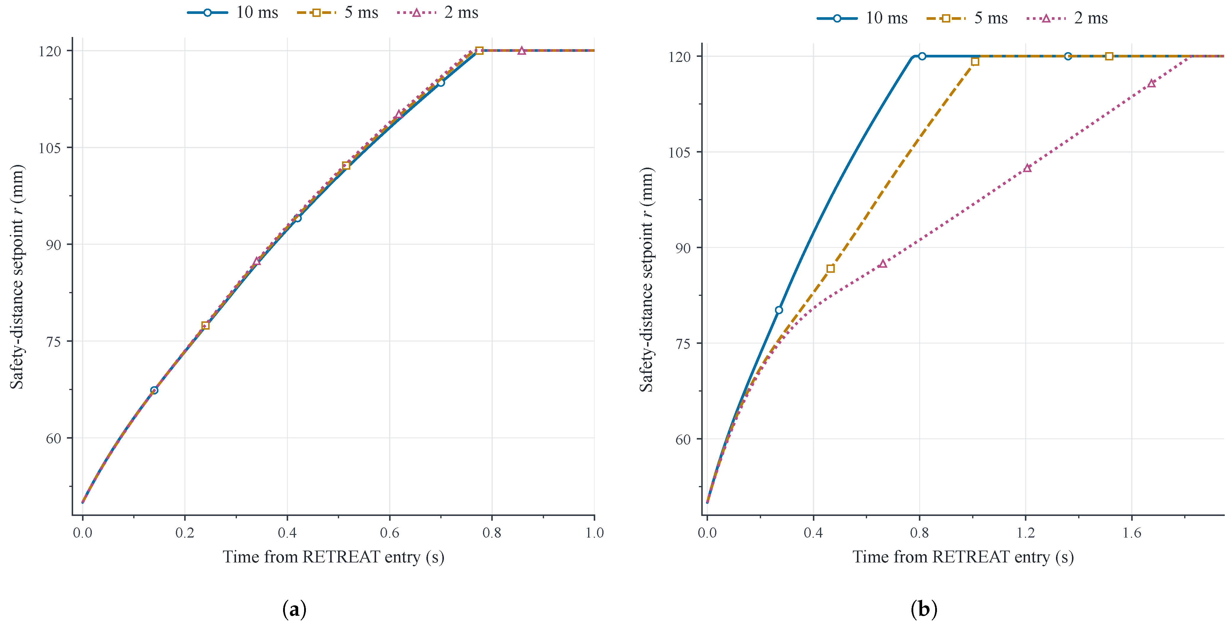
Fixed-$\theta$ and sampling-aware tuning were compared at $T_s=10$, 5, and 2 ms. The full-task study covered six scenarios, three tuning constants, and two tuning designs at these three control periods, giving 108 logical cells. Removing duplicate settings left 78 unique physical trajectories. All 78 runs completed. The maximum relative recovery-time deviation fell from 296.634% with fixed tuning to 7.143% with sampling-aware tuning.

In a second experiment, three stored RETREAT states served as matched initial conditions. Only the control period and corresponding tuning were changed. All 15 physical continuations completed. The maximum deviation fell from 1.368 s (201.176%) to 0.012 s (1.714%). Table 1 summarizes both tests.

Table 1. Recovery-time sensitivity to the control period under fixed-$\theta$ and sampling-aware tuning.

Study	Fixed max. dev. [s]	Fixed rel. dev. [%]	Sampling-Aware max. dev. [s]	Sampling-Aware rel. dev. [%]
Full-task grid	2.996	296.634	0.070	7.143
Matched RETREAT initial conditions	1.368	201.176	0.012	1.714

Figure 8 shows a representative matched RETREAT initial condition. The other two stored states showed the same qualitative pattern: fixed-$\theta$ tuning varied substantially with the control period, whereas sampling-aware tuning produced a more consistent recovery response.

Figure 8. Recovery responses from a representative matched RETREAT initial condition. (a) Sampling-aware tuning. (b) Fixed-$\theta$ tuning.

We varied only c from the same saved C3 RETREAT state at $T_s=10$ ms (Table 2). All three runs completed. Increasing c slowed recovery and increased the point-wise capacity reserve, but the measured geometric clearance decreased. No integration substep in these runs violated the fixed distance floor or requested setpoint. These sampled checks do not establish safety between updates.

Table 2. C3 Python sensitivity to c from one saved state at $T_s=10$ ms. Reserve is minimum ${\kappa }_k-{\nu }_k$; clearance is minimum substep inter-arm distance minus $r_k$, both during active recovery.

c [${\mathbf{s}}^{-1}$]	$\mathit{\theta }$	${\mathit{T}}_{\mathbf{rec}}$ [s]	Min. Reserve [mm/s]	Min. Clearance [mm]
2.5	0.975	0.69	1.995	2.326
5	0.950	0.75	3.426	1.771
10	0.900	1.00	5.987	0.748

These results demonstrate that sampling-aware tuning provides more consistent recovery responses across the tested control periods, although it does not guarantee sampling-independent behavior.

We also varied the CBF gains one at a time in the full C3 Python task. With ${\beta }_0=8{\mathrm{s}}^{-1}$, setting $\beta$ to 2, 4, and $8{\mathrm{s}}^{-1}$ gave recovery times of 0.73, 0.75, and 0.82 s. The minimum geometric margins during active recovery were 8.018, 1.771, and 0.322 mm, respectively. Changing ${\beta }_0$ to 4, 8, or $16{\mathrm{s}}^{-1}$ with $\beta =4{\mathrm{s}}^{-1}$ did not change the C3 trajectory, since the fixed minimum-distance constraint was inactive. All five runs completed without recorded distance-constraint violations or LP/QP failures. These single runs show sensitivity in C3, but it does not show optimal gains or continuous-time safety.

5.4. Matched Comparison of Recovery Policies

Five recovery policies were compared under matched conditions: Time-linear, Entry-certified, Direct-rate, Step, and the proposed Per-cycle capacity-feedback policy. The five cases varied the task offset, $v_{\max }$, $\overline{a}$, and $\overline{\nu }$. Within each case, all policies started from the same pre-policy RETREAT state and used the same physical constraints. Step changed the setpoint instantaneously from $r_c$ to $r_n$. For this comparison, Direct-rate used ${\lambda }_{\nu }={10}^5$, ${\nu }_{\mathrm{ref}}=\overline{\nu }$, and $k_{\mathrm{req}}=0.02$.

Time-linear used $T_R=(r_n-r_c)/\overline{\nu }$, so its planned rate equaled the case’s rate cap. Entry-certified used the same $\theta =0.95$ and cap as Proposed but held its entry rate fixed; Step applied the immediate setpoint change. Direct-rate used ${\nu }_{\mathrm{ref}}=\overline{\nu }$ and $k_{\mathrm{req}}=0.02{\mathrm{s}}^{-1}$ to favor fast, positive progress. Its original weight ${\lambda }_{\nu }={10}^5$ was a fixed project setting rather than an optimized value. We also tested ${10}^4$ from the same saved states, changing only this weight and using the same cold-start QP protocol in all five cases. No method was tuned separately for each case.

The cases represent high fixed-rate demand (C1), reduced joint-velocity authority (C2), restrictive velocity and acceleration limits (C3), low available capacity under limited acceleration (C4), and combined high-rate stress (C5).

Table 3 gives the cold-start results. Proposed completed all five cases; Entry-certified became infeasible in C3. Direct-rate reached the QP iteration limit at ${\lambda }_{\nu }={10}^5$ but completed all five cases at ${10}^4$. Thus, its original terminations do not show that the method itself is infeasible.

Table 3. C1–C5 cold-start recovery results. Times denote completed recovery; “QP limit” denotes final solver termination rather than mathematical infeasibility. Direct-rate used the same weights across cases.

Case	Time- Linear	Entry- Certified	Step	Direct-Rate ${\mathit{\lambda }}_{\mathit{\nu }}={10}^5$	Direct-Rate ${\mathit{\lambda }}_{\mathit{\nu }}={10}^4$	Proposed
C1	QP infeasible	0.44 s	QP infeasible	QP limit	0.34 s	0.36 s
C2	QP infeasible	0.42 s	QP infeasible	QP limit	0.34 s	0.39 s
C3	QP infeasible	QP infeasible	QP infeasible	QP limit	0.67 s	0.75 s
C4	QP infeasible	0.80 s	QP infeasible	QP limit	0.47 s	0.60 s
C5	QP infeasible	0.63 s	QP infeasible	QP limit	0.34 s	0.34 s

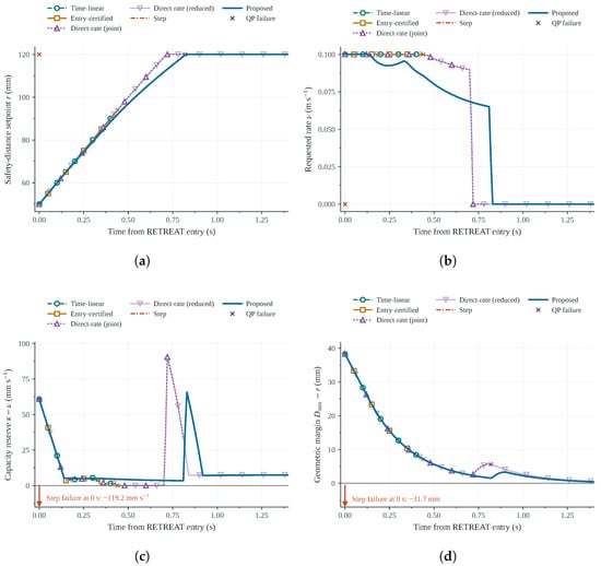
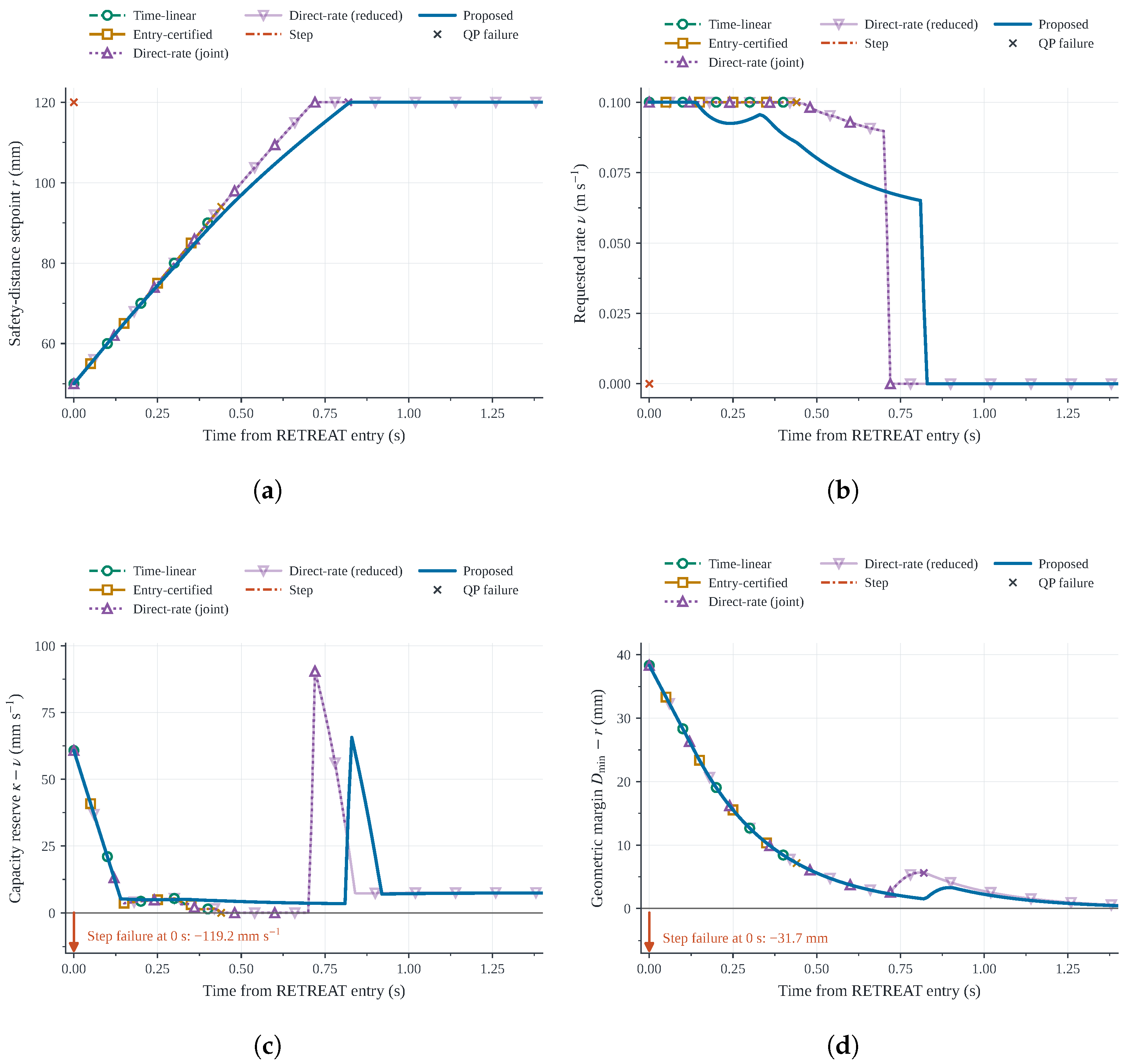
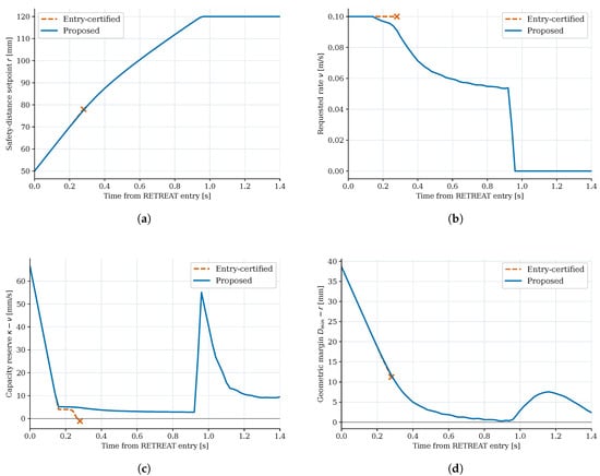
Figure 9 compares the C3 recovery trajectories of the five policies, including both Direct-rate weighting settings. The original Direct-rate setting with ${\lambda }_{\nu }={10}^5$ reached the QP iteration limit, whereas the reduced-weight setting with ${\lambda }_{\nu }={10}^4$ completed recovery. Table 3 reports the corresponding results across C1–C5.

Figure 9. Comparison of five recovery policies in Case C3. The Direct-rate curves correspond to ${\lambda }_{\nu }={10}^5$ (original) and ${\lambda }_{\nu }={10}^4$ (reduced), using cold-start QP solves. (a) Safety-distance setpoint. (b) Requested rate. (c) Capacity reserve. (d) Geometric margin.

In C3, Direct-rate with ${\lambda }_{\nu }={10}^4$ completed recovery in 0.67 s compared with 0.75 s for Proposed. The proposed method instead makes the feasible-rate threshold explicit and updates it each cycle rather than keeping the entry rate fixed as Entry-certified does. These comparisons describe the tested settings and do not establish an overall speed advantage.

The proposed controller solves one capacity LP and one motion QP per cycle, while Direct-rate solves one QP. For the 14-joint model and 49 cross-arm collision pairs, the proposed LP has 15 variables and the QP has 14. Given the computed geometry and Jacobians, forming the collision-constraint coefficients takes $O\left(mn\right)$ time for m pairs and n joints; this does not include LP or QP solution time.

We measured Python controller time in three repeats from the same saved C3 state at $T_s=10$ ms. Over the first 40 successful cycles shared by Proposed, Entry-certified, Time-linear, and Direct-rate, the median times were 2.951, 2.051, 2.054, and 1.929 ms, respectively. Step stopped at entry and could not be compared over this interval. The measurement includes geometry, constraint construction, and the required solver calls but excludes integration and logging. This limited test does not establish worst-case or hardware real-time performance.

5.5. Physics-Based Closed-Loop Validation in Isaac Sim

We further evaluated the proposed controller in NVIDIA Isaac Sim to verify whether the recovery mechanism observed in the Python simulation persists under rigid-body dynamics and measured-state feedback. We retained the same task-level recovery formulation but replaced the velocity-level state update with a PhysX-based rigid-body simulation incorporating articulation-drive dynamics and measured-state feedback. The robot was modeled as a 14-DoF dual-arm articulation with the geometry, mass, and inertial properties of each link defined in a Universal Scene Description (USD) model.

At each control cycle, the controller received the measured joint positions and velocities from Isaac Sim, evaluated the current collision geometry and feasibility capacity, selected the recovery rate, and solved the same motion-control QP described in Section 4. Subsequently, the resulting joint-velocity commands were transmitted to the simulated articulation, and Isaac Sim fed the measured states obtained through rigid-body dynamics back to the controller. The purpose of this verification was not to accurately reproduce the trajectories of the velocity-level simulation but to confirm whether the core capacity-feedback mechanism remained effective when actuator-tracking effects and rigid-body dynamics were included.

Figure 10 shows the Isaac Sim environment and the dual-arm robot model used for the physics-based validation.

Figure 10. Isaac Sim environment for physics-based validation. (a) Dual-arm robot model. (b) Representative task scene.

In the Python simulation, the limitation of entry-certified recovery was most clearly observed in Case C3. This case was therefore selected for the physics-based validation. Under the velocity and acceleration limits imposed in C3, the entry-certified policy became infeasible after entering the RETREAT phase, whereas the proposed policy successfully completed the recovery. We examined whether this qualitative difference persisted when rigid-body dynamics, actuator-tracking effects, and measured-state feedback were included in the Isaac Sim environment.

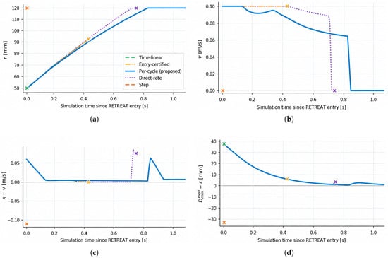
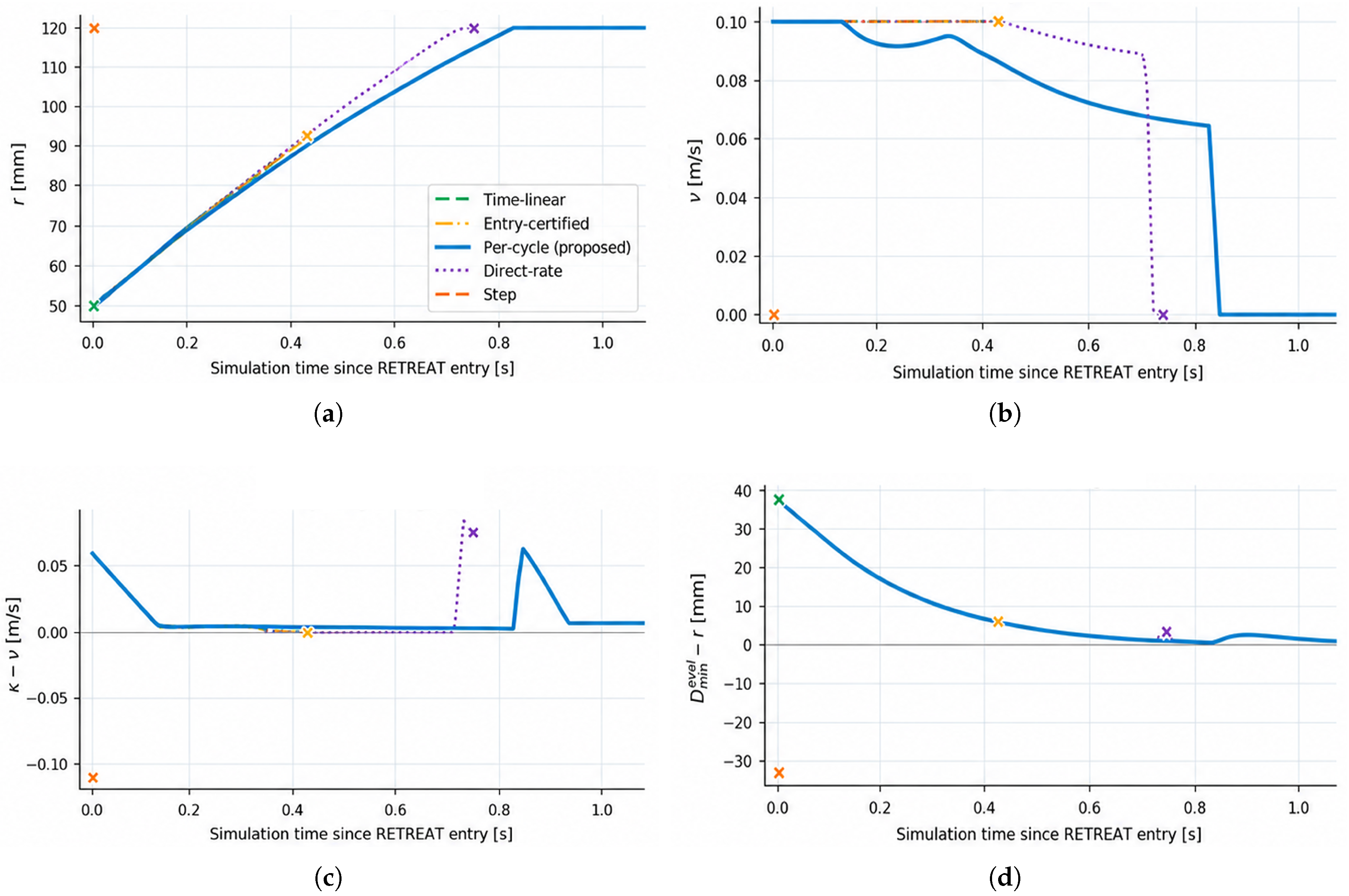
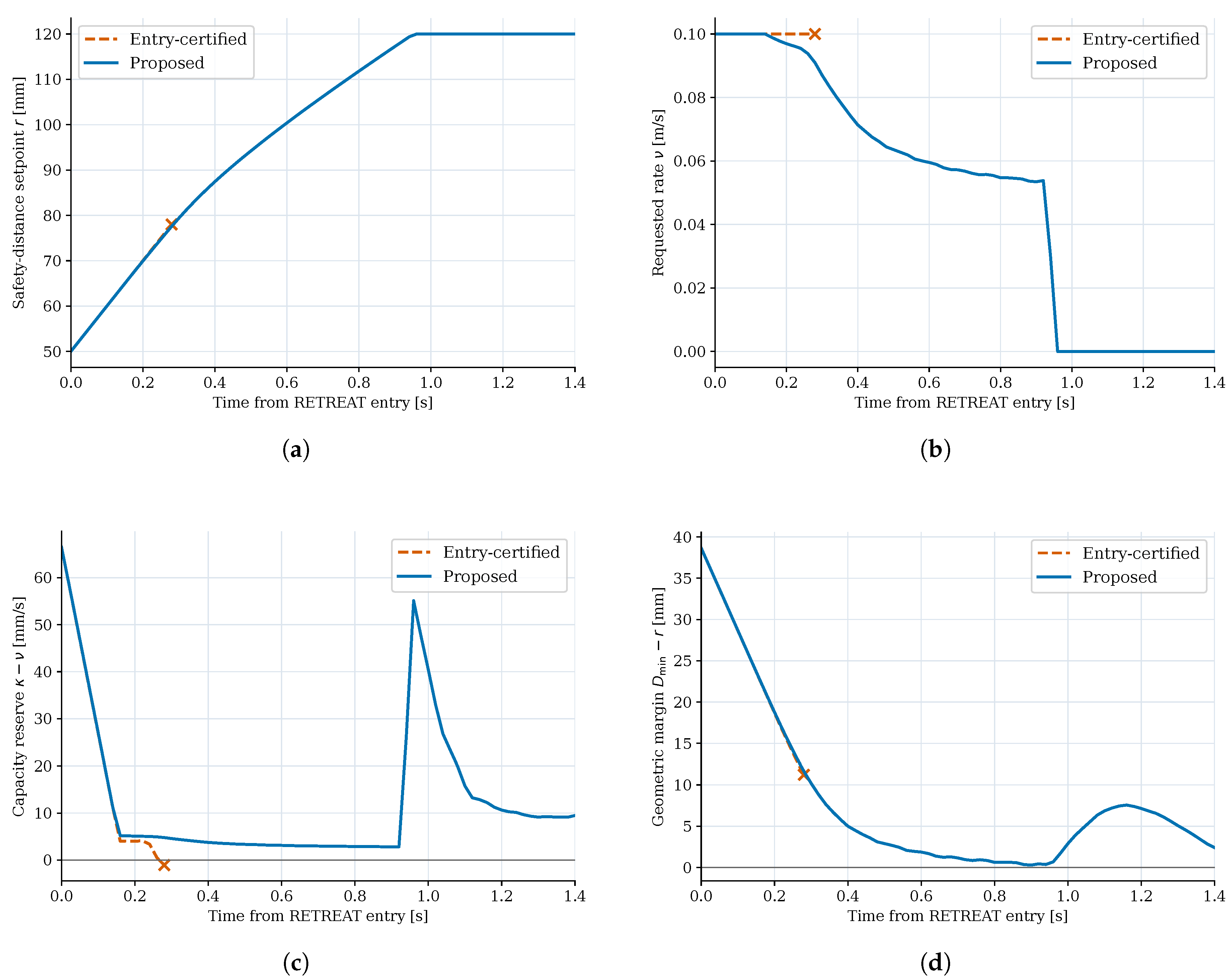
During the validation, the proposed per-cycle capacity-feedback policy and the entry-certified fixed-rate policy were compared under identical C3-based conditions. Figure 11 plots the C3 responses of the policies identified in its legend; the quantitative comparison here focuses on the proposed and entry-certified policies. The proposed controller recalculated the instantaneous feasibility capacity at each control cycle and adjusted the required recovery rate accordingly. In contrast, the entry-certified policy maintained the fixed recovery rate determined at RETREAT entry.

Figure 11. Isaac Sim C3 recovery responses for the policies shown in the legend; the quantitative comparison focuses on the proposed and entry-certified policies. Colored crosses indicate policy termination points. (a) Safety-distance recovery. (b) Capacity and requested rate. (c) Capacity reserve. (d) Geometric margin.

The proposed policy completed the safety-margin recovery with $T_{\mathrm{rec}}=0.760$ s while maintaining a minimum point-wise capacity reserve of $3.370$ mm/s. In contrast, the point-wise capacity reserve of the entry-certified policy decreased to $-0.144$ mm/s, after which execution was terminated because the control QP became infeasible. These results are consistent with the key mechanism observed in the C3 rate study. In other words, even if the recovery rate is feasible at RETREAT entry, it does not necessarily remain feasible because the closed-loop state and the admissible control set evolve over time.

The minimum geometric margin measured under the proposed policy was $-0.697$ mm. Although this value was slightly below zero, it remained within the 5 mm geometric tolerance used as the recovery criterion throughout the numerical evaluation. The capacity reserve indicates the point-wise feasibility of the velocity-level recovery constraint rather than an actuator-level robustness margin. Therefore, even if the point-wise capacity reserve remains positive, small deviations between the prescribed safety distance and the actual minimum distance measured in the rigid-body simulation may occur due to actuator-tracking errors and dynamic effects.

Table 4 summarizes the quantitative results for the two policies. Here, NR indicates that the nominal recovery condition was not reached before the solver terminated. The geometric margin is defined as $D_{\min }-r$, and the capacity reserve is defined as $\kappa -\nu$.

Table 4. Isaac Sim results under Case C3.

Method	Outcome	${\mathit{T}}_{\mathbf{rec}}$ [s]	Min. Geometric Margin [mm]	Min. Capacity Reserve [mm/s]
Entry-certified	QP infeasible	NR	6.688	−0.144
Proposed	Completed	0.760	−0.697	3.370

Overall, the Isaac Sim results show that the qualitative capacity-feedback behavior observed in the velocity-level simulation was maintained under the tested physics-based closed-loop conditions. The proposed policy completed the C3-based recovery by adjusting the requested recovery rate according to the instantaneous feasibility capacity, whereas the entry-certified policy lost point-wise feasibility after RETREAT entry. These results provide additional validation under rigid-body dynamics and measured-state feedback.

5.6. Experimental Validation on the Physical Robot

5.6.1. Experimental Setup and Evaluation Method

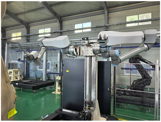
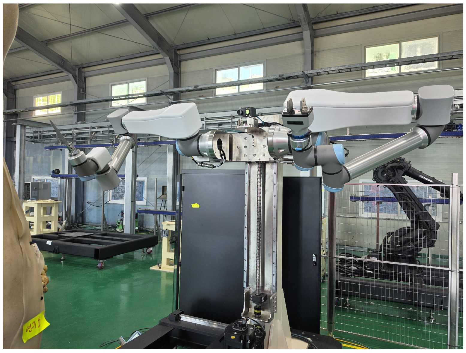
To evaluate whether the capacity-feedback mechanism for safety-margin recovery observed in simulation remained effective on the physical robot, experiments were conducted on a 14-DoF bimanual system comprising two six-axis UR robots and an auxiliary (AUX) rotary axis for each arm, as shown in Figure 12. At each control cycle, the controller used the measured joint states to compute the current collision geometry and instantaneous feasibility capacity and generated joint-velocity commands for the selected recovery rate. The physical-robot experiments used the C3-based hardware constraints with a control period of 20 ms. The capacity-scaling factor was fixed at $\theta =0.95$ in all trials.

Figure 12. Physical setup of the 14-DoF bimanual grasp-and-cut system.

The experiments consisted of a policy comparison in the baseline configuration and repeated recovery tests with changes in the task configuration. For the baseline comparison, the proposed per-cycle capacity-feedback policy and the entry-certified fixed-rate policy were each executed five times under the C3-based hardware constraints. For the configuration study, the proposed policy was executed five times in each of four configurations: the baseline configuration, configurations with both task locations translated by $-250$ mm and $+250$ mm along the Y axis, and a configuration with the knife positioned horizontally above the gripper. The baseline trials of the proposed policy were used in both evaluations, giving a total of 25 distinct trials.

The physical-robot experiments followed the task sequence described in Section 2.1 and used the recovery criterion defined in Section 5.1. The minimum distance $D_{\min }$ was computed from the measured joint angles using the capsule model.

5.6.2. Repeated Policy Comparison in the Baseline Configuration

The policy comparison in the baseline configuration examined whether the difference between the proposed and entry-certified policies observed in Section 5.4 and Section 5.5 was also observed on the physical robot. Both policies used the same task targets and admissible control constraints and differed only in the recovery-rate selection method used during RETREAT. Figure 13 compares the five-trial mean responses of the two policies.

Figure 13. Five-trial mean responses of the proposed and entry-certified policies under C3-based hardware constraints. Colored crosses indicate policy termination points. (a) Safety-distance recovery. (b) Requested rate. (c) Capacity reserve. (d) Geometric margin.

The proposed policy satisfied the recovery criterion in all five trials with a mean recovery time of $0.860$ s. In contrast, the solver reported the motion-control QP under the entry-certified policy as infeasible, and execution terminated approximately $0.28$ s after RETREAT entry in every trial before the recovery criterion was reached.

The proposed policy adjusted the requested recovery rate according to the instantaneous feasibility capacity, whereas the entry-certified policy maintained the rate selected at RETREAT entry. The requested rate under the entry-certified policy was 100 mm/s, but the feasibility capacity computed at the termination instant of each trial had decreased to $98.641$–$99.113$ mm/s. Consequently, the capacity reserve $\kappa -\nu$ became negative, and the solver reported the motion-control QP with that requested rate as infeasible. This is qualitatively consistent with the simulation result that a recovery rate feasible at RETREAT entry is not guaranteed to remain feasible thereafter.

In Table 5, $T_{\mathrm{rec}}$ is the mean recovery time across the five trials. The minimum geometric margin and minimum capacity reserve are the smallest sampled values across all five trials of each policy. The geometric margin is $D_{\min }-r$, and the capacity reserve is $\kappa -\nu$. Geometric margins in both hardware result tables were evaluated at recorded control samples during the first 18 s after RETREAT entry, including the post-recovery period, or until earlier solver termination. The capacity reserve was evaluated at samples with a positive requested recovery rate and a valid LP result, including the final control cycle at which the QP solver reported infeasibility. NR indicates that the recovery criterion was not reached. The positive geometric margin under the entry-certified policy was observed only before early termination and therefore does not indicate better maintenance of the required safety distance than under the proposed policy, which completed the recovery.

Table 5. Repeated policy comparison under C3-based hardware constraints in the baseline configuration on the physical robot.

Method	Successful Recoveries/Trials	Mean ${\mathit{T}}_{\mathbf{rec}}$ [s]	Min. Geometric Margin [mm]	Min. Capacity Reserve [mm/s]
Entry-certified	0/5	NR	$+11.150$	$-1.359$
Proposed	5/5	0.860	$-1.044$	$+2.794$

The minimum geometric margin under the proposed policy was $-1.044$ mm. Thus, the geometric margin was negative at some recorded samples, but the observed deviations remained within the specified 5 mm geometric tolerance. These results demonstrate repeated safety-margin recovery on the physical system under the stated recovery criterion.

5.6.3. Repeated Recovery Performance Under Changes in Task Position and Knife Pose

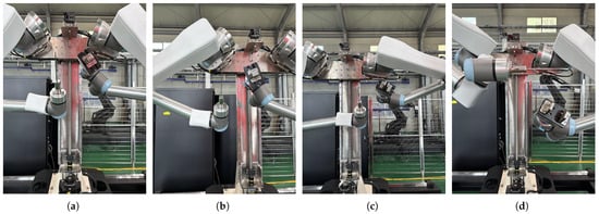
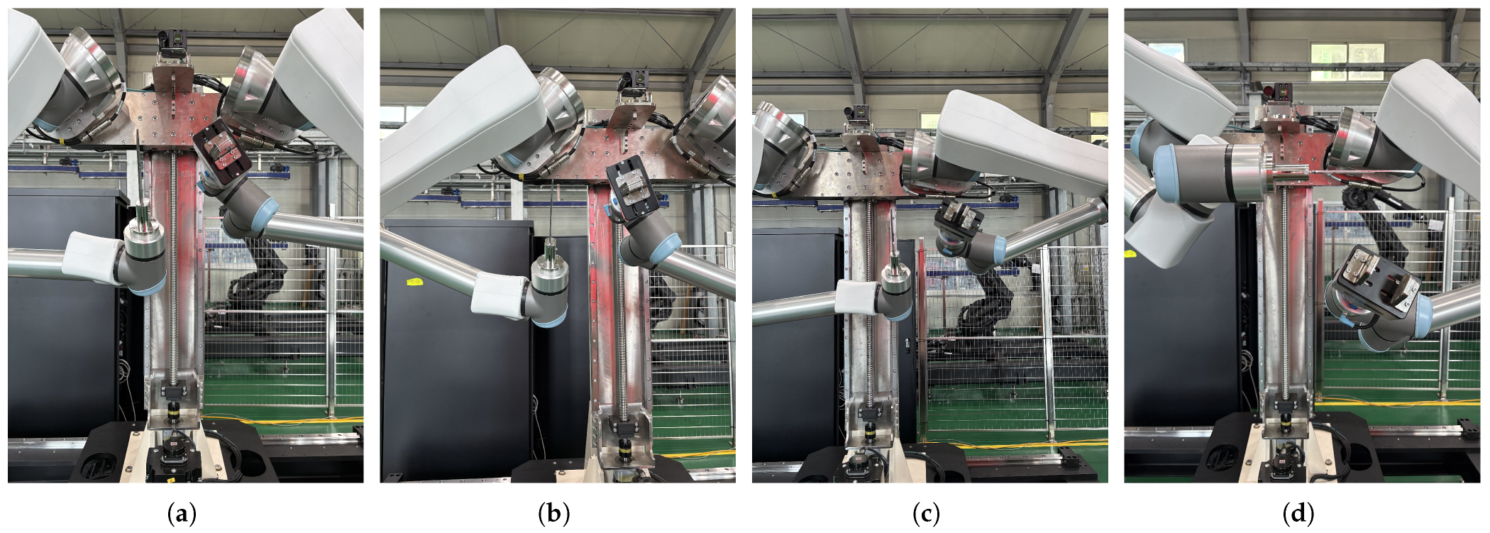
To evaluate recovery performance beyond the baseline task configuration, the proposed policy was repeatedly executed with changes in the grasping and cutting locations and the knife pose. For the position changes, the baseline grasping and cutting points were translated together by $-250$ mm and $+250$ mm along the Y-axis. An additional configuration combined a horizontal knife pose above the gripper with modified grasping and cutting locations. This condition was therefore evaluated as a combined position-and-pose variation rather than an isolated orientation change. The controller parameters and recovery criterion were kept identical across all configurations. Figure 14 shows the four physical task configurations.

Figure 14. Physical task configurations used in the repeated recovery experiments. (a) Baseline configuration. (b) Y − 250 mm translation. (c) Y + 250 mm translation. (d) Horizontal above gripper.

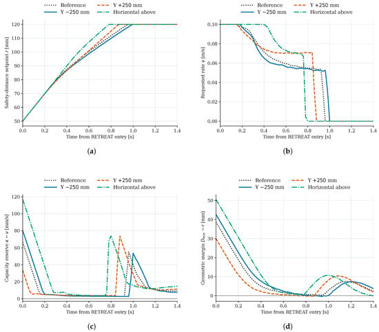
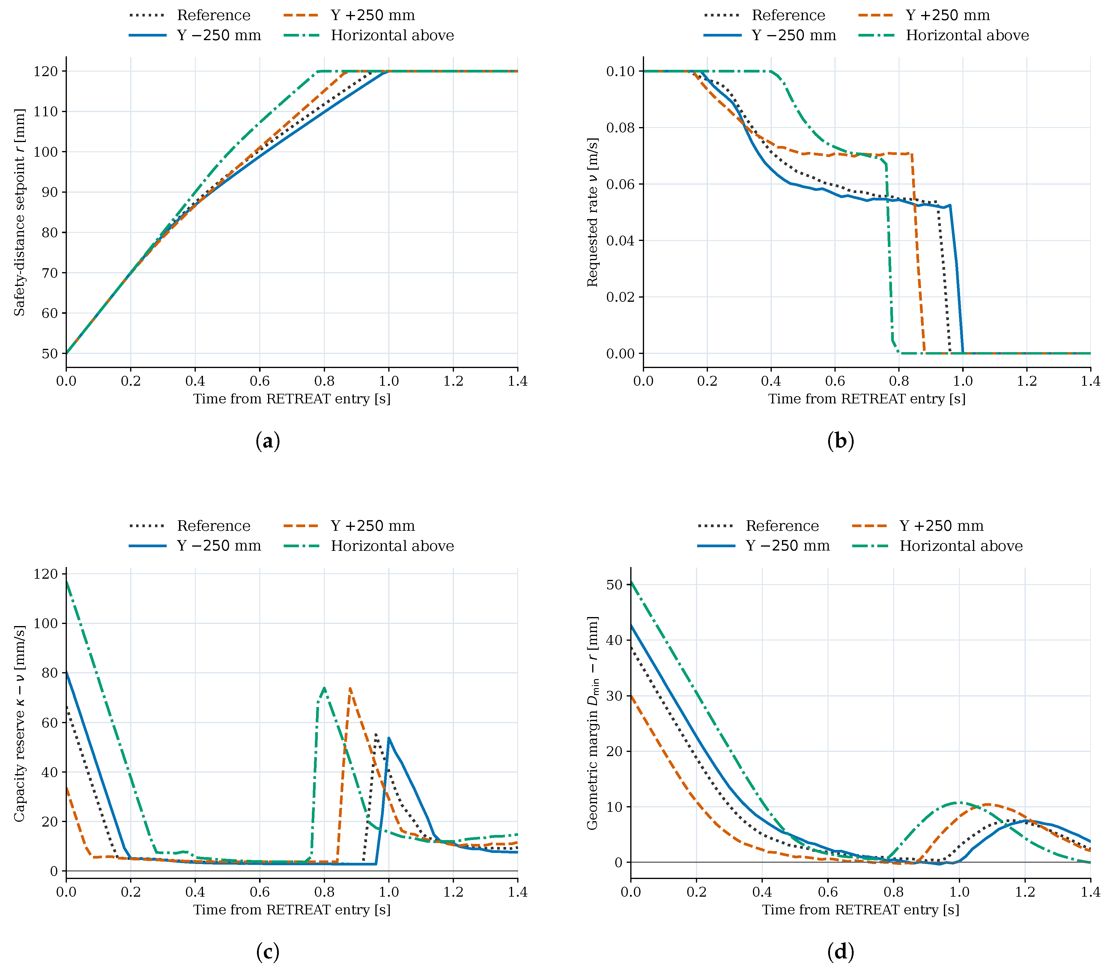
Figure 15 compares the five-trial mean responses across the four configurations. Reference denotes the baseline configuration in the response and deviation plots.

Figure 15. Five-trial mean responses of the proposed policy across four task configurations. (a) Safety-distance recovery. (b) Requested rate. (c) Capacity reserve. (d) Geometric margin.

All five repeated trials satisfied the recovery criterion in each of the four configurations. The mean recovery times were $0.860$ s in the baseline configuration, $0.900$ s and $0.800$ s for the Y-axis translations of $-250$ mm and $+250$ mm, respectively, and $0.720$ s for the configuration with the knife horizontal above the gripper. Although the time histories of feasibility capacity and requested recovery rate varied with the configuration, the proposed policy completed recovery in every trial.

The geometric margins and capacity reserves in Table 6 are the minimum values across the five trials in each configuration. The capacity reserves were evaluated using the same positive-rate and valid-LP criteria as in Table 5. In every configuration, the minimum capacity reserve during active recovery was positive, and the observed negative geometric margins remained within the 5 mm tolerance. These results show that the proposed policy repeatedly completed safety-margin recovery under the evaluated changes in task position and knife pose.

Table 6. Repeated recovery results of the proposed policy under changes in task position and knife pose.

Configuration	Successful Recoveries/Trials	Mean ${\mathit{T}}_{\mathbf{rec}}$ [s]	Min. Geometric Margin [mm]	Min. Capacity Reserve [mm/s]
Baseline	5/5	0.860	$-1.044$	$+2.794$
Y − 250 mm translation	5/5	0.900	$-1.137$	$+2.696$
Y + 250 mm translation	5/5	0.800	$-1.371$	$+3.655$
Horizontal above gripper	5/5	0.720	$-0.829$	$+3.590$

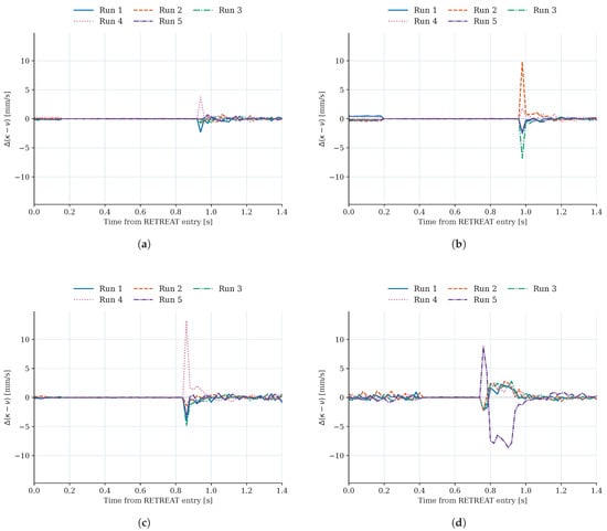
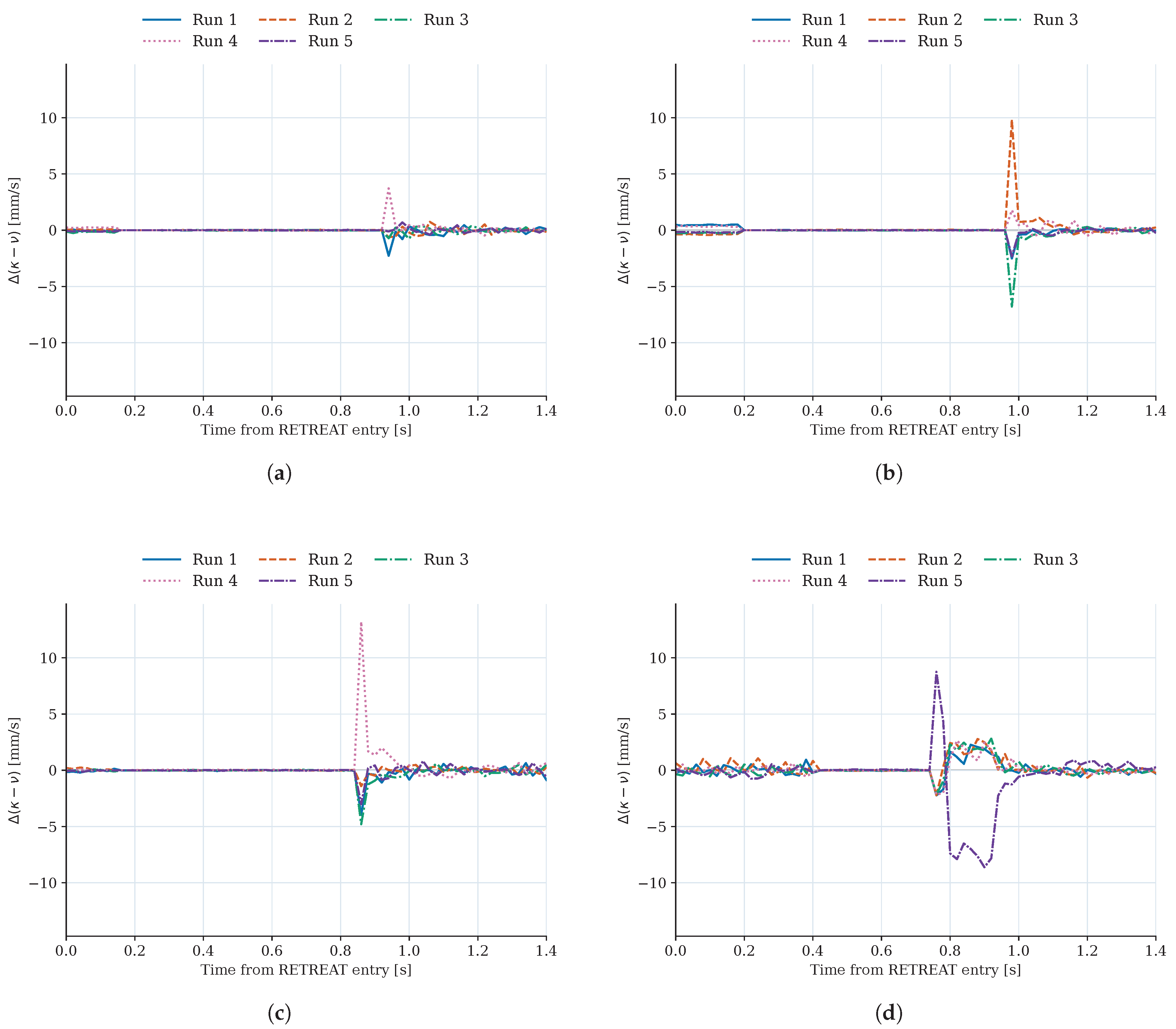
The five recovery times in each configuration were identical at the 20 ms recording resolution, but the detailed responses were not identical. Differences in the capacity reserve across repeated trials can be observed in the deviations from the five-trial mean presented in Figure 16. Deviations were calculated by subtracting the five-trial mean at each corresponding sample from each trial’s capacity reserve; negative deviations do not necessarily indicate negative capacity reserves. These experiments support repeated recovery in the selected task configurations; they do not establish performance guarantees for arbitrary task locations or the entire workspace.

Figure 16. Trial-to-trial deviations of the capacity reserve from the five-trial mean under the proposed policy. (a) Baseline configuration. (b) Y − 250 mm translation. (c) Y + 250 mm translation. (d) Horizontal above gripper.

6. Conclusions

In this study, safety-margin recovery in bimanual grasp-and-cut tasks was formulated as a capacity-feedback control problem. The max–min LP provides an exact point-wise feasibility threshold for the recovery rate under the stated assumptions. Based on this capacity, the proposed per-cycle policy determines the requested recovery rate before solving the motion-control QP. Stored-state tests confirmed the predicted feasibility boundary, while closed-loop simulations showed that a recovery rate selected only at RETREAT entry may become infeasible as the admissible input set changes. In the five matched comparison cases, the proposed policy completed all recoveries, including Case C3, where the entry-certified fixed-rate policy became infeasible.

The sampling-aware tuning rule substantially reduced the dependence of recovery time on the control period in both the full-task study and matched RETREAT continuations. These results support the proposed tuning rule over the tested control periods and configurations. The capacity-feedback behavior was also maintained in the Isaac Sim closed-loop validation with rigid-body dynamics and measured-state feedback, where the proposed policy completed the C3-based recovery while the entry-certified policy lost point-wise feasibility.

With the lower tested rate weight, Direct-rate also completed all five Python cases and recovered sooner in C3. The proposed method therefore should not be read as the fastest of the tested policies; its contribution is the explicit, per-cycle calculation of feasible recovery capacity.

Physical-robot experiments further evaluated the recovery mechanism on a 14-DoF bimanual system at a control period of 20 ms under C3-based hardware constraints. In the baseline configuration, the proposed policy achieved recovery in all five trials, with a mean recovery time of 0.860 s, whereas all five entry-certified trials terminated before reaching the recovery criterion. The proposed policy also achieved recovery in all five trials for each of three additional task configurations with mean recovery times of 0.900, 0.800, and 0.720 s. These results demonstrate repeated recovery under the evaluated task-position and knife-pose variations.

The capacity result concerns sampled states and does not ensure safety between updates. The Python model excludes self-collision, environmental contact, and tissue interaction. The timing measurements cover controller calculations in a limited Python test but not worst-case execution or hardware real-time performance.

References

- Ames, A.D.; Xu, X.; Grizzle, J.W.; Tabuada, P. Control Barrier Function Based Quadratic Programs for Safety Critical Systems. IEEE Trans. Autom. Control 2017, 62, 3861–3876. [Google Scholar] [CrossRef] [Scilit]
- Ames, A.D.; Coogan, S.; Egerstedt, M.; Notomista, G.; Sreenath, K.; Tabuada, P. Control Barrier Functions: Theory and Applications. In Proceedings of the 2019 18th European Control Conference (ECC), Naples, Italy, 25–28 June 2019; pp. 3420–3431. [Google Scholar]
- Parwana, H.; Panagou, D. Rate-Tunable Control Barrier Functions: Methods and Algorithms for Online Adaptation. In Proceedings of the 2025 American Control Conference (ACC), Denver, CO, USA, 8–10 July 2025; pp. 275–282. [Google Scholar]
- Xiao, W.; Belta, C.; Cassandras, C.G. Adaptive Control Barrier Functions. IEEE Trans. Autom. Control 2022, 67, 2267–2281. [Google Scholar] [CrossRef] [Scilit]
- Zeng, J.; Zhang, B.; Li, Z.; Sreenath, K. Safety-Critical Control Using Optimal-Decay Control Barrier Function with Guaranteed Point-Wise Feasibility. In Proceedings of the 2021 American Control Conference (ACC), New Orleans, LA, USA, 25–28 May 2021; pp. 3856–3863. [Google Scholar]
- Breeden, J.; Panagou, D. Compositions of Multiple Control Barrier Functions Under Input Constraints. In Proceedings of the 2023 American Control Conference (ACC), San Diego, CA, USA, 31 May–2 June 2023; pp. 3688–3695. [Google Scholar]
- Tan, X.; Dimarogonas, D.V. Compatibility Checking of Multiple Control Barrier Functions for Input Constrained Systems. In Proceedings of the 2022 IEEE 61st Conference on Decision and Control (CDC), Cancun, Mexico, 6–9 December 2022; pp. 939–944. [Google Scholar]
- Chen, Y.; Jankovic, M.; Santillo, M.A.; Ames, A.D. Backup Control Barrier Functions: Formulation and Comparative Study. In Proceedings of the 2021 60th IEEE Conference on Decision and Control (CDC), Virtual, 14–17 December 2021; pp. 6835–6841. [Google Scholar]
- Parwana, H.; Black, M.; Hoxha, B.; Okamoto, H.; Fainekos, G.; Prokhorov, D.; Panagou, D. Feasible Space Monitoring for Multiple Control Barrier Functions with Application to Large Scale Indoor Navigation. In Proceedings of the 2025 IEEE Conference on Control Technology and Applications (CCTA), San Diego, CA, USA, 25–27 August 2025; pp. 171–178. [Google Scholar]
- Sah, C.K.; Keshavan, J. Exact Feasibility Certification and Optimal Responsibility Allocation for Multi-Robot CBF Safety Filters. arXiv 2026, arXiv:2609.14935. [Google Scholar]
- Igarashi, M.; Tezuka, I.; Nakamura, H. Time-Varying Control Barrier Function and Its Application to Environment-Adaptive Human Assist Control. IFAC-PapersOnLine 2019, 52, 735–740. [Google Scholar] [CrossRef] [Scilit]
- Freire, V.; Nicotra, M.M. Using Dynamic Safety Margins as Control Barrier Functions. IEEE Trans. Autom. Control 2026, 71, 5908–5919. [Google Scholar] [CrossRef] [Scilit]
- Gadginmath, D.; Allibhoy, A.; Pasqualetti, F. Constricting Tubes for Prescribed-Time Safe Control. IEEE Control Syst. Lett. 2026, 10, 679–684. [Google Scholar] [CrossRef] [Scilit]
- Chen, Y.; Cassandras, C.G.; Xiao, W.; Li, A. Exact-Time Safety Recovery Using Time-Varying Control Barrier Functions with Optimal Barrier Tracking. arXiv 2026, arXiv:2603.19119. [Google Scholar]
- Garone, E.; Di Cairano, S.; Kolmanovsky, I.V. Reference and Command Governors for Systems with Constraints: A Survey on Theory and Applications. Automatica 2017, 75, 306–328. [Google Scholar] [CrossRef] [Scilit]
- Garone, E.; Nicotra, M.M. Explicit Reference Governor for Constrained Nonlinear Systems. IEEE Trans. Autom. Control 2016, 61, 1379–1384. [Google Scholar] [CrossRef] [Scilit]
- Li, Z.; Atanasov, N. Governor-Parameterized Barrier Function for Safe Output Tracking with Locally Sensed Constraints. Automatica 2023, 152, 110996. [Google Scholar] [CrossRef] [Scilit]
- Nakano, S.; Garone, E.; Notomista, G. Optimization-Free Constrained Control with Guaranteed Recursive Feasibility: A CBF-Based Reference Governor Approach. arXiv 2026, arXiv:2604.04001. [Google Scholar]
- Rauscher, M.; Kimmel, M.; Hirche, S. Constrained Robot Control Using Control Barrier Functions. In Proceedings of the 2016 IEEE/RSJ International Conference on Intelligent Robots and Systems (IROS), Daejeon, Republic of Korea, 9–14 October 2016; pp. 279–285. [Google Scholar]
- Wang, L.; Ames, A.D.; Egerstedt, M. Safety Barrier Certificates for Collisions-Free Multirobot Systems. IEEE Trans. Robot. 2017, 33, 661–674. [Google Scholar] [CrossRef] [Scilit]
- Kaypak, A.U.; Wei, S.; Krishnamurthy, P.; Khorrami, F. Safe Multi-Robotic Arm Interaction via 3D Convex Shapes. Robot. Auton. Syst. 2026, 196, 105263. [Google Scholar] [CrossRef] [Scilit]
- Cabral Muchacho, R.I.; Laha, R.; Pokorny, F.T.; Figueredo, L.F.C.; Chakraborty, N. Unifying Complementarity Constraints and Control Barrier Functions for Safe Whole-Body Robot Control. IEEE Trans. Autom. Control 2026, 1–17. [Google Scholar] [CrossRef] [Scilit]
- Wilkinson, M.; Bahati, G.; Bena, R.M.; Fourney, E.; Burdick, J.W.; Ames, A.D. Full-Body Dynamic Safety for Robot Manipulators: 3D Poisson Safety Functions for CBF-Based Safety Filters. arXiv 2026, arXiv:2604.21189. [Google Scholar]
- Kouidri, I.; Dahmani, A.; Bailek, N.; Mouni, L.; Sharkawy, A.N. Enhanced Safety in Industrial Robots: An Optimized Hybrid Method for External Torque Prediction. Int. J. Robot. Control Syst. 2026, 6, 401–422. [Google Scholar] [CrossRef] [Scilit]
- Agrawal, A.; Sreenath, K. Discrete Control Barrier Functions for Safety-Critical Control of Discrete Systems with Application to Bipedal Robot Navigation. In Proceedings of the Robotics: Science and Systems, Cambridge, MA, USA, 12–16 July 2017. [Google Scholar]
- Breeden, J.; Garg, K.; Panagou, D. Control Barrier Functions in Sampled-Data Systems. IEEE Control Syst. Lett. 2022, 6, 367–372. [Google Scholar] [CrossRef] [Scilit]
- Taylor, A.J.; Dorobantu, V.D.; Cosner, R.K.; Yue, Y.; Ames, A.D. Safety of Sampled-Data Systems with Control Barrier Functions via Approximate Discrete Time Models. In Proceedings of the 2022 IEEE 61st Conference on Decision and Control (CDC), Cancun, Mexico, 6–9 December 2022; pp. 7127–7134. [Google Scholar]
- Bahati, G.; Ong, P.; Ames, A.D. Sample-and-Hold Safety with Control Barrier Functions. In Proceedings of the 2024 American Control Conference (ACC), Toronto, ON, Canada, 10–12 July 2024; pp. 5169–5176. [Google Scholar]
- Lumelsky, V.J. On Fast Computation of Distance Between Line Segments. Inf. Process. Lett. 1985, 21, 55–61. [Google Scholar] [CrossRef] [Scilit]
- Huangfu, Q.; Hall, J.A.J. Parallelizing the Dual Revised Simplex Method. Math. Program. Comput. 2018, 10, 119–142. [Google Scholar] [CrossRef] [Scilit]
- Stellato, B.; Banjac, G.; Goulart, P.; Bemporad, A.; Boyd, S. OSQP: An Operator Splitting Solver for Quadratic Programs. Math. Program. Comput. 2020, 12, 637–672. [Google Scholar] [CrossRef] [Scilit]
Disclaimer/Publisher’s Note: The statements, opinions and data contained in all publications are solely those of the individual author(s) and contributor(s) and not of MDPI and/or the editor(s). MDPI and/or the editor(s) disclaim responsibility for any injury to people or property resulting from any ideas, methods, instructions or products referred to in the content. |
© 2026 by the authors. Licensee MDPI, Basel, Switzerland. This article is an open access article distributed under the terms and conditions of the Creative Commons Attribution (CC BY) license.