Development of the LSTM Autoencoder-Based Vibration Anomaly Detection System for CNC Machine

Abstract

This study presents an LSTM autoencoder-based vibration anomaly detection system developed using normal operating data for the servomotor driving the ball screw in a CNC machine tool. The system comprises wireless vibration data acquisition and storage, preprocessing, time series feature generation, model training, and identification of potential anomalies based on reconstruction error (RE). Input features, model architectures, and loss configurations were compared using normal operating data from CNC-A. Vibration RMS and Moving Average were selected as the final input features, together with a loss function incorporating an additional RMS reconstruction error term. The existing standardization parameters and trained models were applied without further adjustment to 29,001 test sequences generated from normal operating data from CNC-B, which had not been used for training or model selection. Across three random seeds, the coefficient of determination (R²) for Vibration RMS was 0.938569 ± 0.000682 across all time steps and 0.931685 ± 0.005062 at the final time step. Potential anomalies were identified using the 99 th percentile (P99) and 99.5 th percentile (P99.5) of the RE distribution derived from the CNC-A normal validation data. The proportion of CNC-B test sequences exceeding P99 ranged from 2.121% to 2.262%, and 567 sequences (1.955%) were identified by all three models. This study demonstrates the implementation and application of a system that transfers models trained on normal operating data and validation-derived thresholds to a different CNC machine tool to quantify reconstruction discrepancies and identify sequences requiring further examination.

1. Introduction

The Fourth Industrial Revolution has increased the importance of data-driven equipment management in manufacturing [1]. Advances in sensing and information and communications technology (ICT) have enabled the real-time acquisition and analysis of data on the operating conditions of production equipment. These technologies are also used for equipment condition monitoring and maintenance. In particular, computer numerical control (CNC) machine tools are widely used in various manufacturing processes owing to their high machining precision and repeatability. However, prolonged operation, repeated acceleration and deceleration, and variations in load can cause wear and degradation in key components [2]. These changes in equipment condition can lead to reduced machining precision, product defects, and equipment downtime [3].

Industry has traditionally relied on corrective maintenance, in which repairs are performed after a failure occurs, and preventive maintenance, in which inspections are conducted at predetermined intervals. However, corrective maintenance has limited ability to prevent unexpected equipment downtime. Preventive maintenance may result in unnecessary maintenance because it does not adequately account for the actual condition of the equipment. Condition-based maintenance (CBM) has been adopted to address these limitations [4,5,6]. CBM involves analyzing condition data to determine whether maintenance is required. This approach requires anomaly detection techniques that continuously monitor operating conditions and identify deviations from the normal operating range.

Features extracted from measured signals and models such as support vector machines (SVMs), random forests, and artificial neural networks have been used for anomaly detection. Long short-term memory (LSTM) networks have also been investigated for learning temporal relationships in time series data [7,8]. When these models are used in a supervised learning framework to distinguish between normal and faulty conditions, data representing the target conditions and their corresponding labels are required. However, obtaining sufficient data covering diverse fault conditions is challenging in actual production environments, creating a need for anomaly detection methods that learn reference patterns from normal operating data. Autoencoders have also been investigated for equipment condition analysis and anomaly detection. Kim et al. analyzed tool conditions in a CNC machine using a stacked autoencoder [9]. Dou et al. monitored tool wear without explicit condition labels by using RE of cutting force and vibration signals [10]. Yan et al. performed unsupervised anomaly detection by applying a hybrid robust convolutional autoencoder to multisensor data from CNC Machine [11]. Oshida et al. trained a stacked LSTM encoder–decoder on data from normal machining periods and monitored anomalous changes associated with tool wear [12].

Demetgul et al. detected misalignment in linear feed axes using motor current signals and transfer learning [13]. They compared several models, including an LSTM-based autoencoder, to evaluate their ability to distinguish specific anomalous conditions [13]. These studies demonstrate the potential of anomaly detection based on the reconstruction characteristics of vibration and operational data when fault labels are limited. However, differences in the target equipment, input signals, and data conditions make it difficult to determine suitable input configurations and training settings for a specific production environment based solely on existing findings. It is therefore necessary to verify whether the features requested by practitioners contribute to reconstruction performance and to compare feature combinations and model design settings. The effects of model architecture and loss function should be examined alongside the variability arising from repeated training runs. Furthermore, reconstruction performance and threshold exceedance characteristics should be assessed when statistical thresholds established using normal operating data from the machine used for training are applied to another machine.

In this study, an LSTM autoencoder-based vibration anomaly detection system has been developed using vibration data collected during normal operation of a CNC machine tool in an actual production environment, and its application has been evaluated using test data. To this end, a workflow was established comprising data preprocessing, time series feature generation, input sequence construction, model training, and the identification of potential anomalies based on reconstruction error. First, the effects of the input features were compared in terms of Vibration RMS reconstruction performance, and the F1 configuration, comprising Vibration RMS and Moving Average, was selected. Repeated training runs were also conducted for different model architectures to compare reconstruction performance and variability across random seeds. The effects of additional weighting in the loss function on reconstruction performance were examined to determine the training settings for the final model. Subsequently, statistical thresholds corresponding to the 99 th and 99.5 th percentiles (P99 and P99.5) were established based on the distribution of reconstruction error (RE) obtained from the normal validation data of CNC-A. Selected final model was then applied to normal operating data from CNC-B, which had not been used for training or model selection. The analysis examined Vibration RMS reconstruction performance, the RE distributions of the validation and test data, and the number and proportion of sequences exceeding the statistical thresholds. Agreement in the identification of potential anomalies among models obtained from repeated training runs was also examined.

2. CNC Machine Anomaly Detection

2.1. CNC Machine

The CNC Machine is production equipment that automatically controls the tool path, spindle speed, and feed rate according to a machining program. Its high positioning accuracy and repeatability enable the precision machining of complex components, supporting its use in various manufacturing sectors. Automation and intelligent technologies have increasingly been applied to CNC machines [14]. Accordingly, condition monitoring and data-driven equipment management using CNC Machine operating data have become increasingly important [14].

The CNC machine comprises a control unit, spindle system, feed system, and tooling system. Among these, the feed system is a key component that controls the position and feed rate of the tool or table. A ball screw feed system comprises components such as a servo motor and a ball screw [15]. The ball screw converts the rotational motion of the servo motor into the linear motion of the table [15]. Zhang et al. reported that the dynamic characteristics of ball screw feed systems are influenced by the mechanical structure and control characteristics [16]. During machining, the feed-axis servo motor undergoes repeated acceleration, deceleration, and changes in direction. The dynamic characteristics of the ball screw feed system may vary with operating position, velocity, and acceleration [16]. These variations can affect the tracking performance and positioning accuracy of the feed system. Liu et al. indicated that dynamic errors in ball screw feed systems can affect positioning accuracy and CNC Machine machining accuracy [17]. In addition, ball screws may experience wear and performance degradation during prolonged repetitive operation. Wu et al. proposed a method for analyzing degradation characteristics and predicting remaining useful life based on changes in ball screw condition [18]. Therefore, continuous monitoring of changes in the condition of the servo motor driving the ball screw and the feed system is needed to identify deviations from normal operating conditions at an early stage.

2.2. Anomaly Detection

Anomaly detection is a method for identifying data that exhibit characteristics differing from typical operating patterns. In industrial equipment, condition data such as vibration, temperature, current, and pressure are analyzed to monitor changes during operation. The purpose of anomaly detection extends beyond collecting measurements to identifying observations that require further examination by analyzing deviations from reference operating patterns. Changes in equipment condition can lead to reduced machining precision, product defects, and equipment downtime. Addressing these issues requires continuous monitoring of operating conditions and the identification of deviations from the established operating range. Anomaly detection identifies the times and intervals at which changes in equipment warrant attention, providing information to support inspection and maintenance. In actual production environments, obtaining sufficient data on diverse fault conditions and accurate condition labels is particularly challenging. These limitations constrain methods that classify equipment conditions using fault data, highlighting the need for approaches that identify changes relative to patterns learned from normal operating data.

Anomaly detection methods can be categorized as supervised or unsupervised depending on whether condition labels are used during training [19]. Supervised anomaly detection involves training models on labeled data that distinguish between normal and anomalous conditions. Commonly used classification models include SVMs, random forests, and artificial neural networks. The trained models distinguish between normal and anomalous conditions based on the features of the input data. However, these methods require sufficient fault data and accurate condition labels. In industrial settings, the low frequency of failures makes it difficult to obtain data representing diverse anomalous conditions. Unsupervised anomaly detection learns data distributions and patterns without using condition labels. After learning the characteristics of operational data, these methods identify observations that deviate substantially from established patterns as potential anomalies [20]. In autoencoder-based methods, the model is trained to reconstruct the input data. When normal operating data are used for training, the RE, defined as the difference between the input and its reconstruction, can be used to assess deviations from the learned patterns. This approach enables changes in equipment condition to be monitored relative to normal operating patterns even when fault data are limited.

3. Development of the CNC Machine Tool Anomaly Detection System

3.1. Anomaly Detection System Architecture

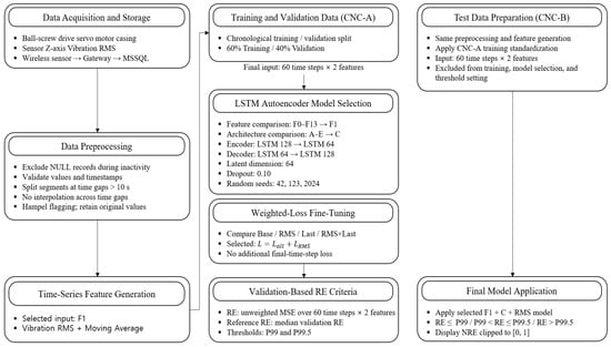
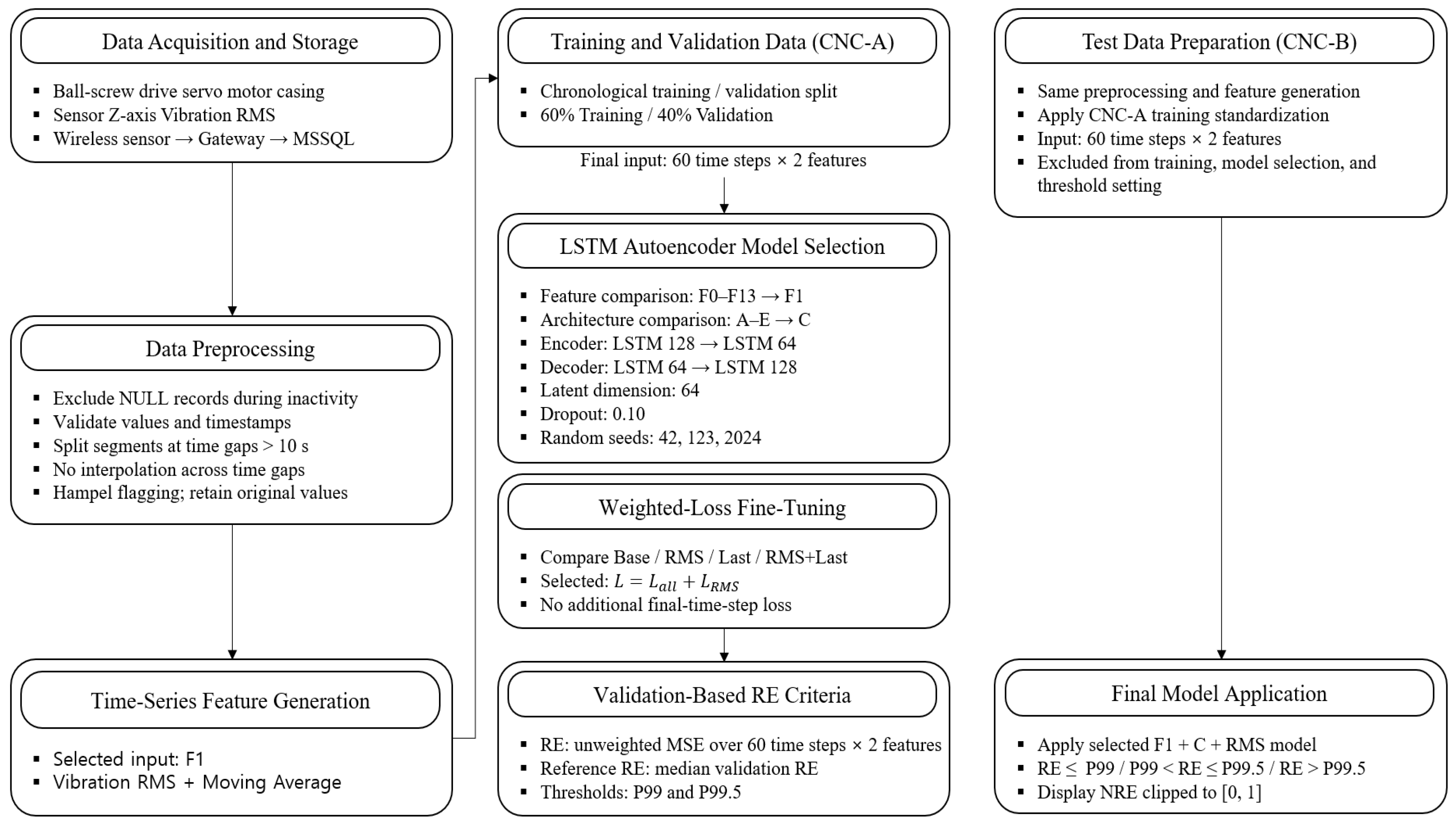
In this study, an LSTM autoencoder-based vibration anomaly detection system was developed for the servomotor driving the ball screw in a CNC machine tool. The system learns normal operating patterns and identifies changes that deviate from those patterns. The development workflow comprised data acquisition and storage, preprocessing, candidate feature generation and selection, model training, and identification of potential anomalies based on reconstruction error. Operational requirements were incorporated into the model input configuration and analysis procedures, and key design settings were examined through comparative experiments. The overall system architecture is shown in Figure 1.

Figure 1. Anomaly Detection System Architecture.

Vibration RMS (root mean square) along the Z-axis of the sensor coordinate system was collected using a wireless vibration sensor attached to the external casing of the servomotor. The measurement timestamps and RMS values were transmitted through a gateway and stored in a Microsoft SQL Server (MSSQL) database. NULL records associated with equipment inactivity were excluded, and the data were divided into separate continuous segments whenever the interval between consecutive valid measurements exceeded 10 s. Time gaps were not bridged by interpolation, and potential outliers flagged by the Hampel identifier were retained at their original values without removal or replacement.

Six candidate features—Vibration RMS, Moving Average, Standard Deviation, Slope, ΔRMS, and Growth Rate—were generated within each continuous segment. The effects of adding individual features and the reconstruction performance of different feature combinations were compared. A subsequent comparison of the final candidates using the full datasets led to the selection of F1, comprising Vibration RMS and Moving Average, as the final input configuration. Normal operating data from CNC-A were divided chronologically into training and validation datasets. Standardization parameters for each feature were calculated exclusively from the training data and applied unchanged to the validation and test data. Input sequences were constructed from 60 measurement time points within each continuous segment of each dataset, resulting in a final model input shape of 60 time steps and two features.

The LSTM autoencoder consisted of an encoder that compressed each input sequence into a latent vector and a decoder that reconstructed the sequence from this vector. Architecture C was selected by comparing validation RE and Vibration RMS reconstruction performance across model architectures under the same F1 input configuration. The selected encoder comprised LSTM layers with 128 and 64 units, yielding a 64-dimensional latent vector. The decoder repeated the latent vector over 60 time steps and reconstructed the input through LSTM layers with 64 and 128 units. Dropout with a rate of 0.10 was applied between the LSTM layers in both the encoder and decoder. The comparative experiments were repeated using random seeds of 42, 123, and 2024 to examine reconstruction performance and variability across runs.

Using the selected architecture, the base MSE loss was compared with loss functions that assigned additional weight to Vibration RMS reconstruction and reconstruction at the final time step. The RMS configuration was adopted for final training, adding a Vibration RMS reconstruction error term across all time steps to the MSE for both input features. The coefficients of the base loss term and the additional RMS loss term were each set to 1, and no additional final-time step loss term was included. This formulation retained the reconstruction objective across the entire input while assigning additional weight to reconstruction of Vibration RMS, the primary measured variable.

Potential anomalies were identified using RE, calculated separately from the weighted training loss as the mean squared error between the standardized input and reconstructed values across all 60 time steps and both features. The median RE of the normal validation data was defined as the Reference RE, and the 99.0 th and 99.5 th percentiles of the RE distribution were adopted as the P99 and P99.5 thresholds, respectively. Test sequences were categorized into three intervals: at or below P99, above P99 but at or below P99.5, and above P99.5. Sequences exceeding P99 were defined as potential anomalies requiring further examination. Normalized reconstruction error (NRE) was also used to display the relative error magnitude and its variation over time by mapping the Reference RE to 0 and P99.5 to 1 and clipping the resulting values to the range [0, 1].

The final model was applied to normal operating data from CNC-B, which had not been used for training, selection of input features or model settings, or for establishment of statistical thresholds. The standardization parameters derived from the CNC-A training data and the RE thresholds established using the normal validation data were applied unchanged to CNC-B. Vibration RMS reconstruction performance, the RE distribution, and the characteristics of sequences reaching or exceeding the statistical thresholds were evaluated using normal operating data from this different machine. This evaluation examined the model’s behavior when applied to normal operating data; sequences reaching or exceeding the thresholds were not regarded as confirmed instances of actual faults.

3.2. Data Acquisition

Vibration data were collected from two production CNC machines operating at an industrial site, designated CNC-A and CNC-B. Normal operating data from CNC-A were used for model training and validation. Normal operating data from CNC-B were excluded from training and model selection and used to examine the application of the final model to a different machine.

The measurement target is the servo motor driving the ball screw in each CNC machine. The servo motor is located within an internal equipment panel, which restricts sensor wiring. A wireless vibration sensor was used to minimize interference with equipment operation and machining processes associated with wired measurements. The sensor was magnetically attached to the outer surface of the servo motor casing to minimize structural modifications. A wireless vibration sensor capable of triaxial measurements along the X, Y, and Z axes was used for data acquisition. Vibration RMS measured along the Z-axis of the sensor coordinate system was used as the source signal for generating time series features. RMS represents the overall vibration magnitude over a measurement interval. It is therefore suitable for characterizing overall vibration levels rather than instantaneous values and for tracking changes in vibration over time [19,20]. The stored RMS data were preprocessed and used to calculate candidate features and construct input sequences for the LSTM Autoencoder. The sensor has a maximum acceleration measurement range of $\pm 8\mathrm{g}$ and a resolution of 16 bits. The internal sampling frequency in high-speed measurement mode is 6.4 kHz. The −3 dB bandwidth is 0.1 Hz–3.2 kHz for the X/Y axes and 0.1 Hz–1.8 kHz for the Z-axis. Measurement timestamps and RMS values were transmitted to a gateway via 2.4 GHz wireless communication. The data received by the gateway were forwarded to a server and stored in MSSQL. The median time interval between valid RMS records used in the analysis was approximately 1.827 s. The data acquisition environment and sensor specifications are summarized in Table 1.

Table 1. Data acquisition environment.

Item	Configuration
Measurement target	Servo motor driving the ball screw in the CNC Machine
Sensor type	Triaxial wireless vibration sensor
Measurement axes	X, Y, and Z axes of the sensor coordinate system
Selected variable	Z-axis Vibration RMS
Sensor location	Outer casing of the servo motor
Mounting method	Magnetic mounting
Maximum acceleration measurement range [g]	±8
Resolution [bits]	16
High-speed mode sampling frequency [kHz]	6.4
X-axis −3 dB bandwidth	0.1 Hz–3.2 kHz
Y-axis −3 dB bandwidth	0.1 Hz–3.2 kHz
Z-axis −3 dB bandwidth	0.1 Hz–1.8 kHz
Wireless communication frequency [GHz]	2.4
Median time interval between valid RMS records [s]	1.827
Data transmission path	Vibration sensor → Gateway → Server
Data storage	Microsoft SQL Server (MSSQL)

CNC-A and CNC-B are vertical and horizontal machining centers, respectively, and differ in their structural configurations and key technical specifications. For both machines, the servomotor driving the ball screw was selected as the measurement target. The principal machine specifications and the intended uses of the collected data are summarized in Table 2.

Table 2. Data-Measurement Equipment Specifications.

Parameter	CNC-A	CNC-B
Manufacturer	DN Solutions	DN Solutions
Model	DNM 6700	HC 500
Machine type	Vertical machining center	Horizontal machining center
X-axis travel [mm]	1300	850
Y-axis travel [mm]	670	700
Z-axis travel [mm]	625	750
Maximum spindle speed [r/min]	8000	8000
Maximum spindle power [kW]	18.5	18.5
Maximum spindle torque [N·m]	117.8	-
Tool taper	ISO #40	BT40
Table/pallet size [mm]	1500 × 670	500 × 500
Maximum load capacity [kg]	1300	500
Rapid traverse rate [m/min]	X/Y: 36, Z: 30	-
Data use	Model training/validation Input feature/model setting selection Statistical criteria establishment	Final model reconstruction evaluation

3.3. Data Preprocessing

Data preprocessing was performed before model training because vibration data may contain missing values, duplicate records, and irregular measurement intervals. Measurement timestamps were converted to datetime format, and RMS values were converted to a numeric format. Because RMS is the square root of the mean of the squared vibration signal, it cannot be negative. Accordingly, RMS values that could not be converted to a numeric format or were recorded as negative were treated as invalid. When multiple records shared the same timestamp, only the most recently stored value was retained.

The collected Z-axis Vibration RMS data comprised 2,369,256 records. Of these, 552,216 (23.308%) contained NULL RMS values recorded while the machine was not operating. These records were confirmed not to represent missing measurements caused by communication interruptions or sensor errors. To learn normal operating patterns, the NULL records associated with machine inactivity were excluded from the analysis. This yielded 1,817,040 valid RMS records (76.692%). Further checks identified no records with nonnumeric or negative RMS values, invalid timestamps, or duplicate timestamps. No linear interpolation was performed over the NULL intervals during preprocessing, and no records were generated.

To establish temporally continuous segments within the valid RMS data, a new segment was started whenever the time interval between consecutive measurements exceeded the threshold G.

$$\mathrm{G}=\mathrm{m}\mathrm{a}\mathrm{x}(10,5\mathrm{\Delta }\mathrm{t})$$

(1)

$\Delta t$ denotes the median of the valid measurement intervals. The median measurement interval was 1.827 s, yielding $5\Delta t=9.1355s$. Accordingly, the final time-gap threshold was set to 10 s. Gaps exceeding 10 s were not bridged by interpolation, and the data before and after each gap were assigned to separate continuous segments. Subsequent feature generation and input sequence construction were performed exclusively within each continuous segment. This prevented temporally disconnected measurements from being included in the same sequence.

During CNC machine tool operation, acceleration, deceleration, changes in direction, and load variations can cause abrupt changes in RMS. A Hampel identifier was therefore applied to flag large RMS values for further examination rather than removing them immediately. The Hampel identifier detects local outliers using the median and median absolute deviation (MAD) within a moving window [21]. The window duration was set to approximately 60 s to capture changes in operating conditions rather than short-term measurement fluctuations. This duration corresponds to approximately 33 measurements based on the median measurement interval. Let $x_t$, ${\tilde{x}}_t$, ${\mathrm{M}\mathrm{A}\mathrm{D}}_t$ denote the RMS value at time t, the moving-window median, and the MAD, respectively. Values satisfying the following condition were identified as potential outliers.

$$\mid x_t-{\tilde{x}}_t\mid >5.0 (1.4826 {\mathrm{M}\mathrm{A}\mathrm{D}}_t)$$

(2)

The factor 1.4826 scales the MAD to an estimate of the standard deviation under a normal distribution [21]. The $5.0 \sigma$ threshold is not a fixed requirement of the Hampel method but a criterion selected in this study to identify potential outliers. This relatively conservative threshold was applied to limit excessive flagging of abrupt RMS changes that may occur during actual operation. Values flagged by the Hampel identifier may arise from sensor errors or actual acceleration, deceleration, and load variations. Therefore, these values were marked only as potential outliers, and the original measurements were retained without removal or replacement. This ensured that abrupt vibration changes occurring during actual operation were not arbitrarily excluded from subsequent time series feature generation and anomaly detection. The data preprocessing criteria are summarized in Table 3.

Table 3. Data preprocessing criteria.

Parameter	Criterion
NULL records during machine inactivity	552,216 records (23.308%) excluded
Invalid RMS values	Exclude nonnumeric or negative values (0 records)
Invalid timestamps	0 records
Duplicate timestamps	Retain the last stored value (0 records)
Missing-value interpolation	No linear interpolation applied (0 records)
Time gaps	Split into continuous segments at gaps >10 s
Hampel identifier	Approximately 60 s moving window and a $5.0\sigma$threshold
Potential outliers	Retain original values without removal

3.4. Time Series Feature Generation and Training Data Preparation

3.4.1. Time Series Feature Generation

In accordance with the company’s on-site requirements, six time series features were defined to represent vibration levels, variability, and temporal trends. The candidate features were RMS, moving average, standard deviation, slope, ΔRMS, and growth rate. The Vibration RMS feature used the Z-axis Vibration RMS measured by the sensor, while the remaining five features were calculated from the same signal. The interpretations of the six time series features are summarized in Table 4.

Table 4. Interpretation of time series features.

Feature	Interpretation
RMS	Current vibration RMS measured along the sensor’s Z-axis.
	Indicates increases and decreases in vibration level over time.
Moving Average	Represents the average vibration level over approximately the preceding 60 s.
	Captures the overall vibration level and its changes within a given interval.
Standard Deviation	Represents variability in vibration magnitude over approximately the preceding 60 s.
	Distinguishes periods of stable vibration from those with substantial fluctuations.
Slope	Represents the trend in vibration level over approximately the preceding 60 s.
	Quantifies the trend within the interval using the linear regression slope.
$\Delta$RMS	Represents the change in vibration between the current and preceding measurements.
	Captures abrupt vibration changes between consecutive measurements.
Growth Rate	Represents the relative rate of change with respect to the preceding vibration level.
	Enables comparison of the magnitude of changes relative to the preceding vibration level.

During CNC machine tool operation, RMS values can change abruptly in response to acceleration, deceleration, changes in direction, and load variations. A moving window was applied to calculate Moving Average, Standard Deviation, and Slope, allowing changes in individual measurements to be characterized alongside the mean level, variability, and trend over a given interval. The window size W was set to the number of observations corresponding to approximately 60 s, based on the median measurement interval $\mathrm{\Delta }$t, and was calculated as follows.

$$W=round\left({\displaystyle \frac{60}{\mathrm{\Delta }\mathrm{t}}}\right)$$

(3)

This corresponds to approximately 33 measurements based on the median measurement interval of 1.827 s for the valid data. ΔRMS represents the change in vibration between consecutive measurements. With $x_t$ denoting the RMS value at time t, $\mathrm{\Delta }$RMS was calculated as follows.

$$\mathrm{\Delta }RM{S}_t=x_t-x_{t-1}$$

(4)

Growth rate was defined to represent the relative change in vibration RMS with respect to its value at the preceding time step.

$$GrowthRat{e}_t={\displaystyle \frac{x_t-x_{t-1}}{\mid x_{t-1}\mid }}$$

(5)

The six generated features were used as candidate model inputs. The final input configuration was selected by comparing the effect of adding each feature individually and the reconstruction performance of different feature combinations.

3.4.2. Input Data Preparation

Records for which all six time series features were validly calculated were sorted by measurement timestamp. Normal operating data from CNC-A were split chronologically, with the first 60% used for training and the remaining 40% for validation. This chronological split was adopted because randomly splitting time series data could allow information from later time points to enter the training process. The training data were used to learn the model weights and determine the standardization parameters, whereas the validation data were used to select the input feature combination and model settings and to establish the statistical thresholds. The test dataset comprised vibration data collected during normal operation of CNC-B, a different machine from CNC-A, which provided the training and validation data. For both machines, Z-axis vibration RMS data collected from the external casing of the servomotor driving the ball screw were used. The same preprocessing and feature generation procedures were applied to the CNC-B data. The test data were not used for model training, selection of input features or model settings, or establishment of statistical thresholds. They were used to evaluate the final model’s reconstruction performance and statistical threshold exceedance characteristics.

StandardScaler was applied to account for differences in scale among the features. The mean and standard deviation required for standardization were calculated solely from the CNC-A training data. The same standardization parameters were then applied to the validation and test data. For the original value $x_{t,j}$ of feature j at time t, the standardized value $z_{t,j}$ was calculated as follows.

$$z_{t,j}={\displaystyle \frac{x_{t,j}-{\mu }_j}{{\sigma }_j}}$$

(6)

${\mu }_j$ and ${\sigma }_j$ are the mean and standard deviation of feature j, respectively, calculated from the training data. The standardized data were arranged into input sequences within each continuous segment using a sequence length of 60 and a stride of 9. Measurements from different continuous segments were not included in the same sequence. The composition and purposes of the training, validation, and test datasets are summarized in Table 5.

Table 5. Training, validation, and test data composition.

Dataset	Data	Purpose
Training	First 60% of CNC-A	Model training and scaling
Validation	Last 40% of CNC-A	Model selection and threshold setting
Test	Same measurement location of CNC-B	Final reconstruction and state evaluation

3.4.3. Input Feature Comparison and Selection

A series of comparative experiments was conducted to examine the effects of the six candidate features on Vibration RMS reconstruction performance. Using F0, which included only Vibration RMS, as the baseline, conditions F1–F5 were configured by individually adding moving average, standard deviation, slope, ΔRMS, and growth rate, respectively. All conditions used the same training and validation data and model architecture, with repeated training runs using three random seeds (42, 123, and 2024). Performance under each condition was evaluated using the mean absolute error (MAE), root mean square error (RMSE), and R² for Vibration RMS, and the results were reported as the mean ± standard deviation across the three training runs. The performance comparison results for each input feature combination are summarized in Table 6.

Table 6. Results of the F0–F5 input feature comparison.

Case	Input Features	MAE	RMSE	${\mathit{R}}^{\mathbf{2}}$
F0	RMS	0.103567 ± 0.003425	0.279666 ± 0.001943	0.642965 ± 0.004950
F1	RMS + Moving Average	0.099299 ± 0.001761	0.275546 ± 0.002590	0.653397 ± 0.006523
F2	RMS + Standard Deviation	0.114972 ± 0.004421	0.293657 ± 0.003811	0.606315 ± 0.010254
F3	RMS + Slope	0.108149 ± 0.001737	0.283588 ± 0.001149	0.632887 ± 0.002978
F4	RMS + ΔRMS	0.107550 ± 0.002543	0.273038 ± 0.001787	0.659688 ± 0.004457
F5	RMS + Growth Rate	0.115184 ± 0.003443	0.289587 ± 0.008845	0.616957 ± 0.023583

F1 achieved the lowest MAE of 0.099299, whereas F4 achieved the best RMSE and $R^2$ values of 0.273038 and 0.659688, respectively. In contrast, F2, F3, and F5 showed no improvement in reconstruction performance over F0. As F1 and F4 performed best on different evaluation metrics, F6 was configured to determine whether combining the moving average and ΔRMS would further improve performance. The reconstruction performance results for F6 are summarized in Table 7.

Table 7. Results of the F6 input feature comparison.

Case	Input Features	MAE	RMSE	${\mathit{R}}^{\mathbf{2}}$
F6	RMS + Moving Average + ΔRMS	0.101293 ± 0.003571	0.275056 ± 0.004557	0.654587 ± 0.011496

F6 yielded an MAE of 0.101293 and an RMSE of 0.275056. Although both errors were lower than those of F0, F6 did not simultaneously improve upon the MAE of F1 and the RMSE of F4. These results indicate that increasing the number of features does not necessarily improve reconstruction performance and that performance can vary with the input feature combination. To further examine these effects, the comparison was extended to conditions F7–F13. These conditions included various combinations of moving average, standard deviation, slope, ΔRMS, and growth rate, as well as a configuration using all six features. This enabled a comprehensive assessment of individual feature contributions, changes in reconstruction performance across feature combinations, and variability across repeated training runs. The reconstruction performance comparison results for the F7–F13 input feature combinations are summarized in Table 8.

Table 8. Results of the F7–F13 input feature comparison.

Case	Input Features	MAE	RMSE	${\mathit{R}}^{\mathbf{2}}$
F7	RMS + Moving Average + Standard Deviation	0.107645 ± 0.002579	0.285329 ± 0.002347	0.628353 ± 0.006125
F8	RMS + Moving Average + Slope	0.104384 ± 0.006652	0.281716 ± 0.000507	0.637720 ± 0.001303
F9	RMS + Moving Average + Growth Rate	0.108216 ± 0.002490	0.281821 ± 0.003878	0.637408 ± 0.009987
F10	RMS + Standard Deviation + ΔRMS	0.114257 ± 0.004659	0.289914 ± 0.003201	0.616300 ± 0.008477
F11	RMS + Slope + ΔRMS	0.108854 ± 0.005685	0.280744 ± 0.001688	0.640210 ± 0.004319
F12	RMS + ΔRMS + Growth Rate	0.117812 ± 0.012668	0.287555 ± 0.000919	0.622547 ± 0.002413
F13	All six candidate features	0.106655 ± 0.003957	0.280097 ± 0.001603	0.641867 ± 0.004103

All configurations from F7 to F13 yielded higher mean MAE values than F1, and none achieved a lower mean RMSE than F4. F13, which used all six candidate features, yielded a mean RMSE of 0.280097, slightly higher than the value of 0.279666 obtained with F0. Its mean R² was also lower than that of F0. These results indicate that increasing the number of input features did not necessarily improve Vibration RMS reconstruction performance under the experimental conditions examined.

Based on these comparisons, F1 and F4 were selected as the final candidate input configurations, and an additional comparison was conducted using the full training and validation datasets, with F0, which used RMS alone, included as the baseline. A total of 137,200 training sequences and 29,021 validation sequences were used, with the model architecture and training settings held constant across configurations. Each configuration was trained using random seeds of 42, 123, and 2024. The results of this additional comparison are presented in Table 9.

Table 9. Comparison Results for the F0, F1, and F4 Input Feature Configurations.

Case	Input Features	RMS MAE	RMS RMSE	${\mathit{R}}^{\mathbf{2}}$
F0	RMS	0.068188	0.204208 ± 0.005501	0.808180
F1	RMS + Moving Average	0.061950	0.199993 ± 0.001542	0.816099
F4	RMS + ΔRMS	0.072645	0.203626 ± 0.006520	0.809234

In the comparison using the full datasets, F1 achieved the lowest mean MAE and RMSE of 0.061950 and 0.199993, respectively, and the highest mean R² of 0.816099. Its RMSE standard deviation of 0.001542 was also lower than those of F0 and F4. Accordingly, considering both reconstruction performance and variability across training runs, F1, comprising Vibration RMS and Moving Average, was selected as the final input configuration. The same F1 configuration was used in the subsequent comparisons of model architectures and loss functions.

3.5. LSTM Autoencoder Model Training

3.5.1. LSTM Autoencoder Architecture Configuration

Based on the input feature comparison, the F1 configuration, comprising Vibration RMS and Moving Average, was selected as the final input feature configuration. An LSTM autoencoder was employed to learn the temporal relationships in these time series and reconstruct the input sequences. An autoencoder consists of an encoder that compresses the input data into a latent representation and a decoder that reconstructs the compressed information into the original input format. An LSTM autoencoder incorporates LSTM layers into both the encoder and decoder to learn temporal relationships in time series data. The encoder compresses the temporal features of the input sequence into a latent vector, which the decoder then uses to reconstruct a sequence with the same dimensions as the input [22,23,24].

To examine differences in reconstruction performance across model architectures, the F1 input configuration was held constant while the number of encoder units, latent vector dimensionality, and dropout settings were varied. Each input sequence comprised 60 consecutive measurement time points, with two features at each time point: Vibration RMS and Moving Average. Thus, the input $X_i$ for sequence i is defined as follows.

$$X_i\in {\mathbb{R}}^{60\times 2}$$

(7)

The encoder consisted of two LSTM layers. The first LSTM layer was configured with $return\_sequences=True$ to pass the outputs at all time steps to the next layer, and the final hidden state of the second LSTM layer was used as the latent vector encoding the input sequence. Dropout was applied between the two LSTM layers. In the decoder, RepeatVector was used to repeat the latent vector over 60 time steps, followed by two LSTM layers corresponding to those in the encoder. Finally, a TimeDistributed (Dense (2)) layer reconstructed Vibration RMS and Moving Average at each time step. Thus, the reconstructed sequence ${\widehat{X}}_i$ has the same shape as the input sequence.

$${\widehat{X}}_i\in {\mathbb{R}}^{60\times 2}$$

(8)

Five model configurations were defined, as summarized in Table 10, to compare the effects of model size and dropout rate. In configurations A, B, and C, the dropout rate was fixed at 0.10, while the number of encoder units and the latent vector dimensionality were progressively increased to examine the effect of model size. In configurations B, D, and E, the number of encoder units and the latent vector dimensionality were fixed at 64 and 32, respectively, while the dropout rates were set to 0.10, 0.00, and 0.20 to examine the effect of dropout rate. Configurations A–E were implemented in the code using the same underlying architecture.

Table 10. LSTM autoencoder configurations for architectural comparison.

Condition	Encoder Units	Latent Dimension	Dropout
A	32	16	0.10
B	64	32	0.10
C	128	64	0.10
D	64	32	0.00
E	64	32	0.20

Mean squared error (MSE) was used as the base loss function to account for the overall discrepancy between the input and reconstructed sequences. The reconstruction loss for sequence i was calculated as follows:

$$L_{MSE,i}={\displaystyle \frac{1}{TF}}{\displaystyle \sum _{t=1}^T}{\displaystyle \sum _{f=1}^F}{(X_{i,t,f}-{\widehat{X}}_{i,t,f})}^2$$

(9)

$T=60$ denotes the sequence length, and $F=2$ denotes the number of features. $X_{i,t,f}$ and ${\widehat{X}}_{i,t,f}$ represent the input and reconstructed values, respectively. At this stage, no additional weights were assigned to individual features or time steps, and the model architectures were compared based on reconstruction performance across both input features. The same training and validation datasets were used for all model configurations. The Adam optimizer was used with an initial learning rate of 0.001 and a batch size of 256. Each model was trained for 20 epochs. When the validation loss did not improve for four consecutive epochs, ReduceLROnPlateau reduced the learning rate by a factor of 0.5. For each training run, the model weights from the epoch with the lowest validation loss were saved and restored after training to evaluate validation performance.

To examine the influence of randomness in model initialization on architecture selection, each configuration was trained using random seeds of 42, 123, and 2024. The primary metric for comparing model architectures was validation RE, calculated across both input features: Vibration RMS and Moving Average. MAE, RMSE, and $R^2$ were also calculated for Vibration RMS, the primary measured variable. Results for each configuration were reported as the mean ± standard deviation across the three training runs. Validation RE was calculated by averaging the squared errors across both input features and all 60 time steps. The MAE, RMSE, and $R^2$ for Vibration RMS were calculated using the input and reconstructed Vibration RMS values at all time steps within each validation sequence.

As shown in Table 11, configuration C achieved the lowest mean validation RE of 0.019266 among configurations A–E. It also yielded the lowest MAE and RMSE for Vibration RMS, at 0.059788 and 0.191052, respectively, and the highest R² of 0.832133. Thus, configuration C achieved the best reconstruction performance both across all input features and for Vibration RMS individually.

Table 11. Comparison of LSTM autoencoder architectures under the F1 input configuration.

Condition	Validation RE	RMS MAE	RMS RMSE	R2
A	0.030078 ± 0.001564	0.084504 ± 0.006224	0.238704 ± 0.005736	0.737926 ± 0.012511
B	0.023934 ± 0.001189	0.071584 ± 0.007733	0.213690 ± 0.005453	0.789964 ± 0.010792
C	0.019266 ± 0.000640	0.059788 ± 0.002692	0.191052 ± 0.003981	0.832133 ± 0.007011
D	0.023719 ± 0.000742	0.072325 ± 0.003757	0.212328 ± 0.002964	0.792696 ± 0.005770
E	0.024673 ± 0.001072	0.071475 ± 0.005245	0.216651 ± 0.004733	0.784127 ± 0.009480

Configurations A, B, and C, which were used to examine the effect of model size, showed a decreasing trend in mean validation RE as the number of encoder units and the latent vector dimensionality increased. Validation RE was 0.030078 for A, 0.023934 for B, and 0.019266 for C; the value for C was approximately 19.50% lower than that for B and 35.95% lower than that for A. Vibration RMS RMSE also decreased from 0.238704 for A to 0.213690 for B and 0.191052 for C, while $R^{2}values$ increased to 0.737926, 0.789964, and 0.832133, respectively. In contrast, configurations B, D, and E, all of which used 64 encoder units and a 32-dimensional latent vector, exhibited relatively small performance differences across dropout rates. Their mean validation RE values were 0.023934, 0.023719, and 0.024673, respectively, and their Vibration RMS RMSE values were 0.213690, 0.212328, and 0.216651. Thus, under the experimental conditions examined, changes in model size were associated with larger differences in reconstruction performance than changes in dropout rate. To examine the influence of model initialization, the configurations were ranked by validation RE for each random seed. Configuration C yielded validation RE values of 0.018869, 0.020005, and 0.018924 for seeds 42, 123, and 2024, respectively, achieving the lowest value among the compared configurations for all three seeds. Configuration C therefore achieved the lowest validation RE across all three random seeds used in this comparative experiment, confirming that its selection was consistent across the three initialization settings.

Based on these results, configuration C, comprising 128 encoder units, a 64-dimensional latent vector, and a dropout rate of 0.10, was selected as the final LSTM autoencoder architecture. The weights of the selected model were used to initialize fine-tuning in the subsequent comparison of weighted loss functions. This enabled the effects of the additional loss terms on reconstruction performance to be evaluated across all input features and for Vibration RMS individually. The LSTM Autoencoder architecture and training configuration are summarized in Table 12.

Table 12. LSTM Autoencoder Model Configuration.

Item	Setting
Input Features	Vibration RMS, Moving Average
Input Shape	$60\times 2$
Encoder	LSTM 128 → Dropout 0.10 → LSTM 64
Latent Vector	64 dimensions
Decoder	RepeatVector(60) → LSTM 64 → Dropout 0.10 → LSTM 128
Output Shape	$60\times 2$
Loss Function	MSE
Optimizer	Adam(Adaptive Moment Estimation)
Initial Learning Rate	0.001
Batch Size	256
Epochs	20
Random Seeds	42, 123, 2024
LR Reduction Patience	4 epochs
LR Reduction Factor	0.5

The selected configuration C was trained to minimize the mean squared error across the two input features, Vibration RMS and Moving Average. Because the base MSE averages the squared errors of these features with equal weight, it does not assign additional weight to Vibration RMS, the primary measured variable. Accordingly, the effect of incorporating an additional Vibration RMS reconstruction error term into the loss function was examined. The selected model architecture was retained while the loss function was modified to include this additional term, and the resulting changes in reconstruction performance were compared. Although adding Vibration RMS-related loss terms may improve RMS reconstruction, it may also affect reconstruction performance across all input features. Therefore, the following section compares the base loss configuration with configurations incorporating Vibration RMS-related loss terms to select the final loss function, considering both overall reconstruction performance and Vibration RMS reconstruction performance.

3.5.2. Fine-Tuning Reconstruction Performance Using Weighted Loss

Based on the architecture comparison in the preceding section, configuration C, comprising 128 encoder units, a 64-dimensional latent vector, and a dropout rate of 0.10, was selected as the final LSTM autoencoder architecture. The selected model was trained to reconstruct both input features, Vibration RMS and Moving Average, simultaneously. Because the base loss function averages the RE of both features, the effect of assigning additional weight to the RE of Vibration RMS, the primary analysis variable measured directly by the sensor, was examined. First, the RE across all 60 time steps and both input features was defined as the base $L_{all,i}$.

$$L_{all,i}={\displaystyle \frac{1}{TF}}{\displaystyle \sum _{t=1}^T}{\displaystyle \sum _{f=1}^F}{(X_{i,t,f}-{\widehat{X}}_{i,t,f})}^2$$

(10)

$T=60$ denotes the sequence length, and $F=2$ denotes the number of input features. $X_{i,t,f}$ and ${\widehat{X}}_{i,t,f }$are the input and reconstructed values, respectively. $L_{all,i }$represents the RE over the entire input sequence, including both Vibration RMS and Moving Average. Vibration RMS represents the vibration level measured directly by the sensor and was used as the primary analysis variable in this study. Accordingly, $L_{RMS,i}$ was defined as follows to incorporate an additional Vibration RMS reconstruction error term while retaining the reconstruction objective across all input features.

$$L_{RMS,i}={\displaystyle \frac{1}{T}}{\displaystyle \sum _{t=1}^T}{(X_{i,t,1}-{\widehat{X}}_{i,t,1})}^2$$

(11)

The feature index $f=1$ denotes Vibration RMS. $L_{RMS,i}$ does not replace $L_{all,i}$; instead, it provides an additional loss term that accounts for the Vibration RMS reconstruction error across the entire sequence. The final time step corresponds to the most recent Vibration RMS measurement within the sequence. To examine the effect of placing additional emphasis on the RE at this time step, $L_{Last,i}$ was defined as follows.

$$L_{Last,i}={(X_{i,T,1}-{\widehat{X}}_{i,T,1})}^2$$

(12)

The final loss function was formulated by combining the three loss terms as follows.

$$L_i=\alpha L_{all,i}+\beta L_{RMS,i}+\gamma L_{Last,i}$$

(13)

$\beta$ and $\gamma$ are the coefficients that assign additional weight to the Vibration RMS reconstruction errors across all time steps and at the final time step, respectively. The coefficient of the base loss $L_{all,i}$ was fixed at 1, and the inclusion of $\beta$ and $\gamma$ was varied to isolate and compare the effects of the individual loss terms. Accordingly, four configurations—Base, RMS, Last, and RMS + Last—were defined, as summarized in Table 13. Base used only the base MSE across both input features. The RMS configuration added the Vibration RMS error across all time steps, whereas the Last configuration added only the Vibration RMS error at the final time step. The RMS + Last configuration included both additional loss terms. All configurations used the same model architecture C and F1 input features selected in the preceding section.

Table 13. Configurations for comparing weighted loss functions.

Loss Condition	$\mathit{\beta }$	$\mathit{\gamma }$	Composition
Base	0.0	0.0	$L_{\mathrm{a}\mathrm{l}\mathrm{l}}$
RMS	1.0	0.0	$L_{\mathrm{a}\mathrm{l}\mathrm{l}}+L_{\mathrm{R}\mathrm{M}\mathrm{S}}$
Last	0.0	1.0	$L_{\mathrm{a}\mathrm{l}\mathrm{l}}+L_{\mathrm{L}\mathrm{a}\mathrm{s}\mathrm{t}}$
RMS+Last	1.0	1.0	$L_{\mathrm{a}\mathrm{l}\mathrm{l}}+L_{\mathrm{R}\mathrm{M}\mathrm{S}}+L_{\mathrm{L}\mathrm{a}\mathrm{s}\mathrm{t}}$

To assess variability in the results across loss function configurations, each configuration was trained using random seeds of 42, 123, and 2024. All runs used the same training and validation datasets, F1 input features, and model architecture C. Performance for each configuration was reported as the mean ± standard deviation across the three training runs. The loss configurations were evaluated using MAE, RMSE, and $R^2$ for Vibration RMS across all time steps, Vibration RMS RMSE at the final time step, and RE calculated across both input features, Vibration RMS and Moving Average. Because adding an RMS-specific loss term could improve Vibration RMS reconstruction while degrading reconstruction performance across all input features, the final configuration was selected by jointly considering Vibration RMS reconstruction performance and RE across both features.

The comparison results in Table 14 showed that the RMS configuration achieved the best reconstruction performance for both Vibration RMS across all time steps and the two input features overall. RMS MAE and RMSE decreased to 0.049412 and 0.168606, respectively, from 0.051277 and 0.172456 under the Base configuration, while R² increased from 0.863255 to 0.869289. The mean RE across both features also decreased from 0.015409 to 0.015268, and the 95 th percentile of RE decreased from 0.076661 to 0.074267. Based on the mean values reported in the table, RMS RMSE and RE across both features decreased by approximately 2.23% and 0.92%, respectively. Although the improvements were modest, mean reconstruction performance improved for both the primary measured variable, Vibration RMS, and the overall input.

Table 14. Comparison of weighted loss functions.

Loss Condition	RMS MAE	RMS RMSE	R2	Last-Step RMS RMSE	Overall 2-Feature RE	RE P95
Base	0.051277 ± 0.001988	0.172456 ± 0.001406	0.863255 ± 0.002233	0.209307 ± 0.007840	0.015409 ± 0.000283	0.076661 ± 0.001943
RMS	0.049412 ± 0.000247	0.168606 ± 0.001720	0.869289 ± 0.002659	0.196330 ± 0.024250	0.015268 ± 0.000354	0.074267 ± 0.001570
Last	0.054408 ± 0.001612	0.183038 ± 0.003017	0.845937 ± 0.005071	0.033486 ± 0.004196	0.017384 ± 0.000552	0.088513 ± 0.002352
RMS + Last	0.052179 ± 0.001002	0.175673 ± 0.000336	0.858112 ± 0.000543	0.053895 ± 0.007054	0.016269 ± 0.000065	0.082607 ± 0.000472

In contrast, the Last configuration substantially reduced the final-step RMS RMSE from 0.209307 to 0.033486. However, RMS RMSE across all time steps increased from 0.172456 to 0.183038, and RE across both features increased from 0.015409 to 0.017384. These results indicate that directly emphasizing the error at the final time step can improve reconstruction at that time step while degrading reconstruction performance across the entire time series. Similarly, the RMS + Last configuration reduced the final-step RMS RMSE to 0.053895, but its overall RMS RMSE and RE across both features were 0.175673 and 0.016269, respectively, both higher than those of Base. Thus, although the additional final-step loss term effectively reduced the error at that time step, it was excluded from the final loss function after considering overall reconstruction performance.

In this study, the RMS configuration with α = 1, β = 1, and γ = 0 was selected as the final weighted loss function by jointly considering the MAE, RMSE, and R² of Vibration RMS and the mean RE across both input features. Specifically, the final model retained the selected Model C architecture and used the overall reconstruction error of Vibration RMS and Moving Average as the base loss, with an additional term accounting for Vibration RMS reconstruction error across all time steps. The models trained under this configuration were subsequently used to evaluate the test data.

3.6. Identification of Potential Anomalies Based on Reconstruction Error

The final model was trained using a loss function that assigned additional weight to Vibration RMS, whereas potential anomalies were identified using RE, defined as the mean squared error across both input features. For each sequence, RE was calculated from the differences between the standardized input and reconstructed values across all 60 time steps and both input features. RE quantifies the reconstruction discrepancy between the input sequence and the learned reference operating patterns and was used as an indicator of the relative degree of deviation from those patterns. For the two selected input features, Vibration RMS and Moving Average, the RE of sequence i was calculated as follows:

$${RE}_i={\displaystyle \frac{1}{TF}}{\displaystyle \sum _{t=1}^T}{\displaystyle \sum _{f=1}^F}{(X_{i,t,f}-{\widehat{X}}_{i,t,f})}^2$$

(14)

The test dataset comprised data collected during normal operation and contained no labels identifying actual anomalous conditions. Accordingly, the RE-based decision thresholds were defined as statistical criteria for distinguishing relative degrees of deviation from normal operating patterns, rather than as diagnostic thresholds for specific fault conditions. To accommodate the tiered approach to condition management for the target equipment, the 99 th and 99.5 th percentiles of the empirical RE distribution obtained from the normal validation data were adopted as the P99 and P99.5 thresholds, respectively. The median validation RE was also used as the Reference RE, representing the typical reconstruction error level in the validation data.

$${\mathrm{R}\mathrm{E}}_{\mathrm{r}\mathrm{e}\mathrm{f}}=\mathrm{m}\mathrm{e}\mathrm{d}\mathrm{i}\mathrm{a}\mathrm{n}\left({\mathrm{R}\mathrm{E}}^{\mathrm{v}\mathrm{a}\mathrm{l}}\right)$$

(15)

$$T_{99}=Q_{0.99}\left({\mathrm{R}\mathrm{E}}^{\mathrm{v}\mathrm{a}\mathrm{l}}\right),T_{99.5}=Q_{0.995}\left({\mathrm{R}\mathrm{E}}^{\mathrm{v}\mathrm{a}\mathrm{l}}\right)$$

(16)

${\mathrm{R}\mathrm{E}}^{\mathrm{v}\mathrm{a}\mathrm{l}}$ denotes the set of reconstruction errors obtained from the normal validation data, and$Q_p$denotes the p-quantile. Test sequences were categorized into three mutually exclusive intervals: at or below P99, above P99 but at or below P99.5, and above P99.5. Sequences with RE values exceeding P99 were defined as potential anomalies requiring further examination. Among these, sequences exceeding P99.5 were categorized as exceeding the higher statistical threshold. The decision criteria are summarized in Table 15.

Table 15. Reconstruction Error-Based Criteria for Classifying Potential Anomalies.

Category	Decision Criterion	Interpretation
At or below P99	${RE}_i$ ≤ $T_{99}$	Reconstruction error at or below the P99 threshold
Above P99 and at or below P99.5	$T_{99}$ < ${RE}_i\le$ $T_{99.5}$	Potential anomaly exceeding P99 but not P99.5
Above P99.5	${RE}_i>$ $T_{99.5}$	Potential anomaly exceeding the P99.5 threshold

NRE was calculated to express the relative magnitude of RE. The values were transformed by mapping the Reference RE to 0 and the P99.5 threshold to 1, then clipped to the range [0, 1].

$${\mathrm{N}\mathrm{R}\mathrm{E}}_i=min\left[1,\mathrm{m}\mathrm{a}\mathrm{x}(0,{\displaystyle \frac{{\mathrm{R}\mathrm{E}}_{\mathrm{i}}-{\mathrm{R}\mathrm{E}}_{\mathrm{r}\mathrm{e}\mathrm{f}}}{T_{99.5}-{\mathrm{R}\mathrm{E}}_{\mathrm{r}\mathrm{e}\mathrm{f}}}})\right]$$

(17)

NRE was used to examine the relative magnitude of RE and its variation over time. Because all RE values at or above P99.5 are mapped to NRE = 1, NRE alone cannot distinguish a value equal to P99.5 from one exceeding it. Therefore, the original RE values were used to classify sequences according to Table 15 and to assess the magnitude of errors beyond the thresholds.

4. Results and Validation

4.1. Test Data Preprocessing and Feature Extraction Results

Normal operating data from CNC-B were used as the test dataset to evaluate the application of the developed LSTM autoencoder-based vibration anomaly detection system. CNC-B is a separate CNC machine tool that was not used for model training or the selection of input features and model architecture. The final F1 input configuration was applied to the test data, using two features: Vibration RMS and Moving Average. The data were organized into temporally continuous segments, and input sequences of length 60 were generated within each segment. The final test dataset comprised 29,001 sequences generated from 165 continuous segments, with an input shape of (29,001, 60, 2). The median duration of the test sequences was approximately 120.07 s. The standardization parameters established using the CNC-A training data were applied unchanged to the test data. These parameters were not recalculated using CNC-B data, thereby preserving the input transformation used during model training. The test dataset composition is summarized in Table 16.

Table 16. Preprocessing results for the CNC-B test dataset.

Item	Result
Test machine	CNC-B
Number of test sequences	29,001
Sequence length	60 time steps
Number of input features	2
Selected input features	Vibration RMS + Moving Average
Final input shape	(29,001, 60, 2)
Number of continuous segments in the test dataset	165
Median sequence duration	120.07 s
Standardization parameters	Parameters derived from the CNC-A training data

Descriptive statistics for the final input features are presented in Table 17. These statistics were calculated after transforming the Vibration RMS and Moving Average values at the final time step of each test sequence back to their original scale. Vibration RMS had a mean of 9.260198 and a standard deviation of 22.558099. Its median was 4.000000, and its 95 th and 99 th percentiles were 33.000000 and 133.000004, respectively. Moving Average had a mean of 9.231185 and a standard deviation of 19.079085. Its median was 3.818182, and its 95 th and 99 th percentiles were 33.393939 and 114.030300, respectively.

Table 17. Descriptive statistics for the F1 input features in the CNC-B test dataset.

Feature	Mean	SD	Median	P95	P99
Vibration RMS	9.260198	22.558099	4.000000	33.000000	133.000004
Moving Average	9.231185	19.079085	3.818182	33.393939	114.030300

The two features had similar means, but Moving Average exhibited a lower standard deviation and P99 than Vibration RMS. This is consistent with the smoothing effect of the moving average operation on fluctuations in individual measurements.

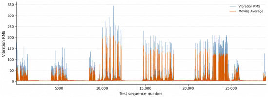
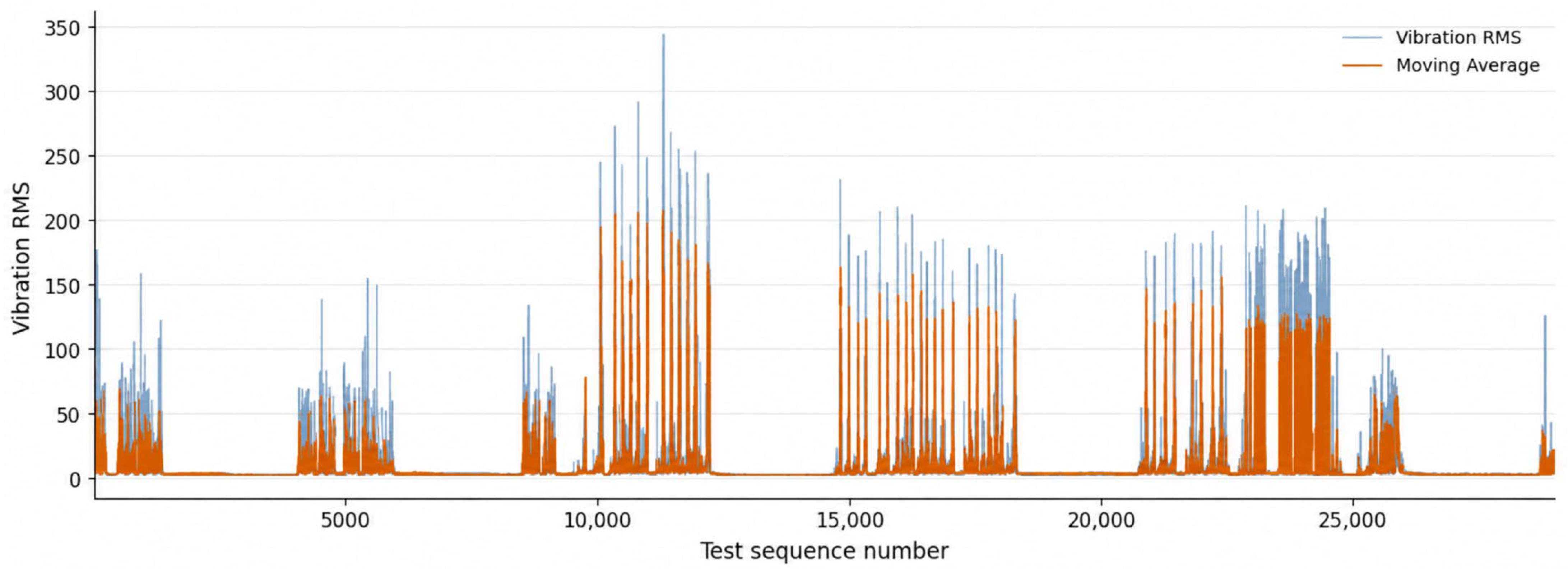
Figure 2 shows the variation in Vibration RMS and Moving Average across the ordered test sequences. Although both features are derived from the same vibration signal, they represent different temporal characteristics. Vibration RMS represents the vibration level at an individual measurement time point, whereas Moving Average represents the average vibration level over a specified time interval.

Figure 2. Temporal variation in Vibration RMS and Moving Average in the CNC-B test dataset.

4.2. Vibration RMS Reconstruction Performance

The final selected LSTM autoencoder model was applied to the CNC-B test dataset to evaluate vibration signal reconstruction performance. The F1 input configuration, comprising Vibration RMS and Moving Average, was used. Each input sequence consisted of 60 time steps and two features. The trained Model C reconstructed the test sequences with the same shape as the input. Vibration RMS was then extracted from the reconstructed features and compared with the measured values.

Model C comprises 128 encoder units, a 64-dimensional latent vector, and a dropout rate of 0.10. The selected RMS loss configuration was used for final training. Evaluation was performed using saved models trained with three different random seeds (42, 123, and 2024). The CNC-B test data were not used for model training or selection. Reconstruction results were therefore obtained by applying the trained models without further training.

Reconstruction performance was evaluated using the MAE, RMSE, and R² for Vibration RMS. Results calculated across all 60 time steps of the test sequences were reported separately from those calculated at the final time step. In the evaluation across all time steps, the same measurement time point may be counted multiple times because of overlapping sequences. Each performance metric was reported as the mean ± standard deviation across the three random seeds. The Vibration RMS reconstruction performance results for the CNC-B test dataset are summarized in Table 18.

Table 18. Vibration RMS reconstruction performance on the CNC-B test dataset.

Evaluation Range	MAE (Mean ± SD)	RMSE (Mean ± SD)	R2 (Mean ± SD)
All time steps	0.054111 ± 0.004158	0.187676 ± 0.001043	0.938569 ± 0.000682
Last time step	0.065660 ± 0.005742	0.198576 ± 0.007427	0.931685 ± 0.005062

Across all time steps, Vibration RMS MAE, RMSE, and R² were 0.054111 ± 0.004158, 0.187676 ± 0.001043, and 0.938569 ± 0.000682, respectively. At the final time step, the corresponding values were 0.065660 ± 0.005742, 0.198576 ± 0.007427, and 0.931685 ± 0.005062. Each metric was reported as the mean ± standard deviation across the three random seeds. The final time step evaluation yielded higher MAE and RMSE and lower R² than the evaluation across all time steps, indicating relatively larger reconstruction errors at the end of each sequence.

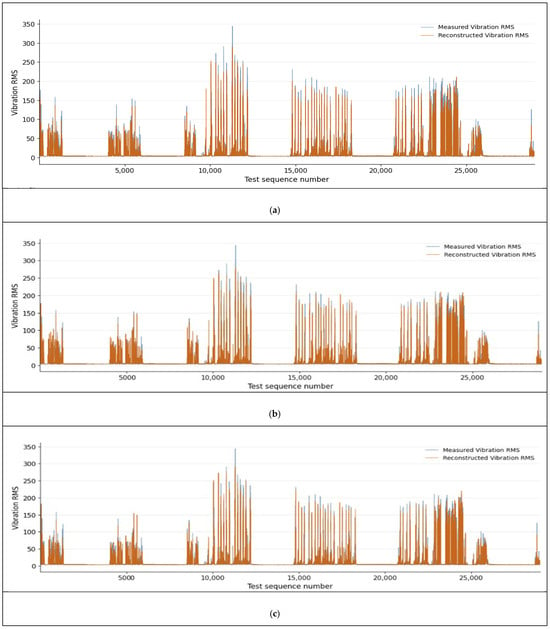
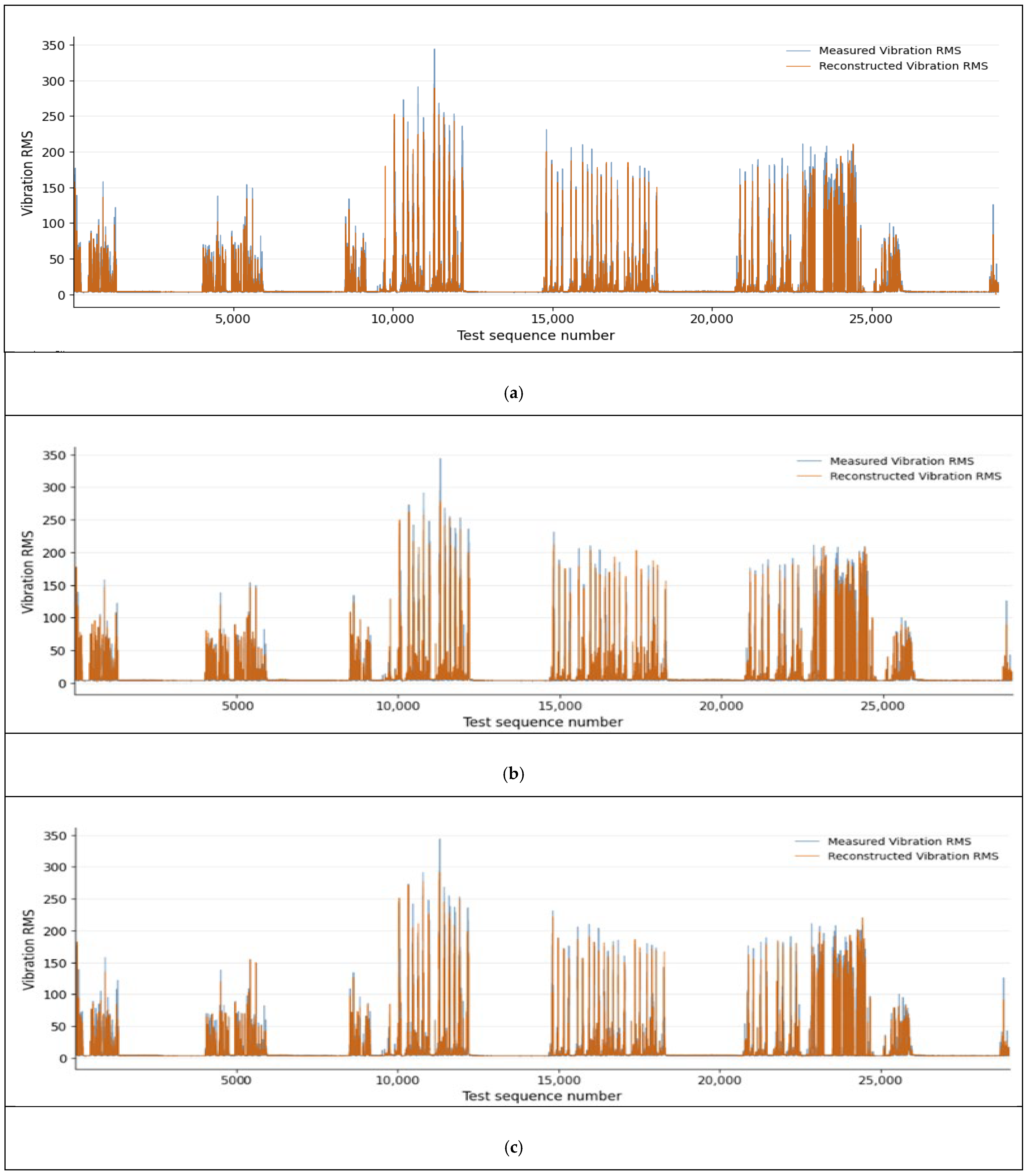
Measured and reconstructed Vibration RMS values were compared to examine how well the models reproduced variations in the test data. Figure 3 presents the results for the three models trained using random seeds of 42, 123, and 2024. The same CNC-B test data were supplied to each model. The measured and reconstructed values at the final time step of each test sequence were transformed back to their original scale and plotted in sequence index order. Identical axis limits were used for all three plots to facilitate comparison of reconstruction patterns across random seeds.

Figure 3. Comparison of measured and reconstructed Vibration RMS over the CNC-B test period for models trained with random seeds (a) 42, (b) 123, and (c) 2024.

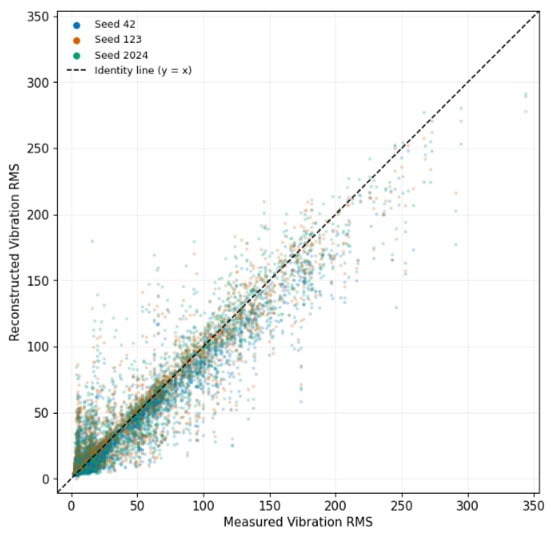
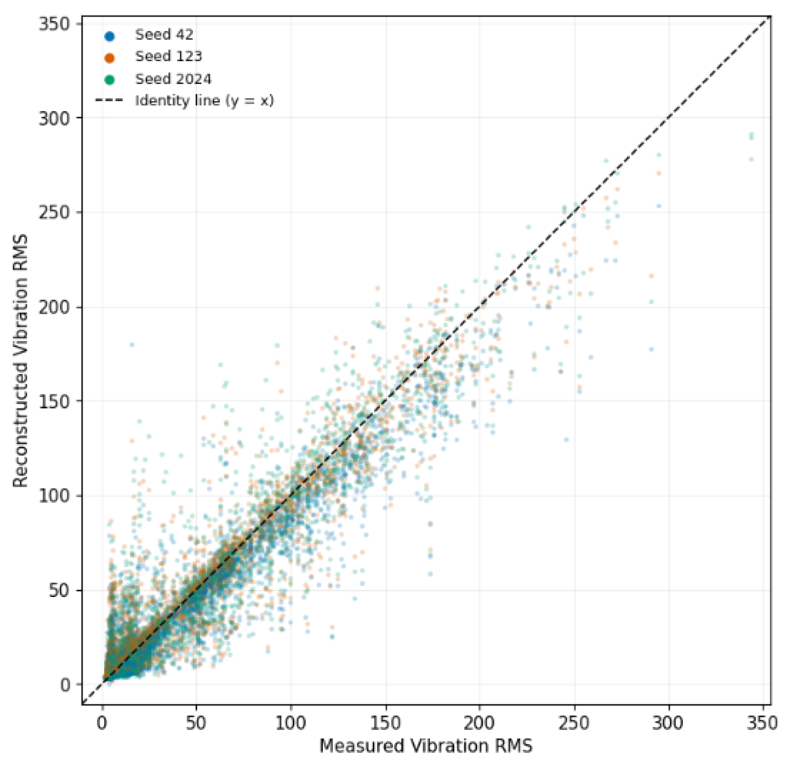
The relationship between measured and reconstructed values is shown in the scatter plot in Figure 4. Results from the three models were overlaid in a single plot, with colors distinguishing the random seeds. The identity line $y=x$ was included to indicate perfect agreement between measured and reconstructed values. This allowed comparison of the distributions of reconstructed values for the same measurements and their deviations from the identity line across models.

Figure 4. Scatter plot of measured and reconstructed Vibration RMS in the CNC-B test dataset for models trained with random seeds 42, 123, and 2024.

These results quantitatively established the reconstruction performance of the final selected model on normal operating data from CNC-B. Comparisons between measured and reconstructed values also revealed how well the model reproduced overall vibration variations and the reconstruction discrepancies at individual measurement points.

4.3. Reconstruction Error Thresholds and Identification of Potential Anomalies

4.3.1. RE Thresholds Derived from Normal Validation Data

Statistical thresholds were established using the RE distribution of the normal validation data from CNC-A. RE was defined as the mean squared error between the standardized input and reconstructed sequences. For each sequence, the squared errors were averaged across all 60 time steps and both input features. This RE served as an indicator for identifying potential anomalies and was distinct from the loss function used for model training. The median of the validation RE distribution was defined as the Reference RE. The 99 th percentile (P99) and 99.5 th percentile (P99.5) were adopted as statistical thresholds for identifying potential anomalies. These values were calculated separately for the model trained with each random seed and applied to the CNC-B test data without further adjustment. The reconstruction error (RE) thresholds derived from the CNC-A normal validation data are summarized in Table 19.

Table 19. RE thresholds derived from the CNC-A normal validation data.

Criterion	Seed 42	Seed 123	Seed 2024	Mean ± SD
Reference RE	0.000399	0.000455	0.000633	0.000496 ± 0.000122
P99	0.271060	0.275027	0.277602	0.274563 ± 0.003296
P99.5	0.410438	0.412497	0.422731	0.415222 ± 0.006584

Across the three random seeds, the Reference RE was 0.000496 ± 0.000122. The mean P99 and P99.5 thresholds were 0.274563 ± 0.003296 and 0.415222 ± 0.006584, respectively. P99 ranged from 0.271060 to 0.277602, and P99.5 ranged from 0.410438 to 0.422731, indicating similar thresholds for identifying potential anomalies across the three random seeds.

4.3.2. RE Distribution and Identification of Potential Anomalies in CNC-B

The statistical thresholds established using the CNC-A normal validation data were applied to the CNC-B test data. The RE distributions of the validation and test datasets were first compared, and the distribution of sequences across the statistical threshold categories was analyzed. Test RE values were calculated independently using the model corresponding to each random seed. Across the three random seeds, the mean RE for the CNC-B test data was 0.019552 ± 0.000072. The RE distributions of the validation and test datasets are presented in Table 20. In this table, SD denotes the standard deviation of sequence-level RE values within each dataset, rather than the standard deviation of the mean RE values across the three seeds.

Table 20. RE distributions of the CNC-A validation data and the CNC-B test data.

Seed	Dataset	Mean	SD	Median	P99	P99.5
42	CNC-A Validation	0.014906	0.073393	0.000399	0.271060	0.410438
42	CNC-B Test	0.019471	0.105397	0.000399	0.445046	0.561878
123	CNC-A Validation	0.015286	0.073151	0.000455	0.275027	0.412497
123	CNC-B Test	0.019607	0.116366	0.000455	0.428673	0.547639
2024	CNC-A Validation	0.015613	0.075223	0.000633	0.277602	0.422731
2024	CNC-B Test	0.019578	0.100182	0.000578	0.434724	0.552312

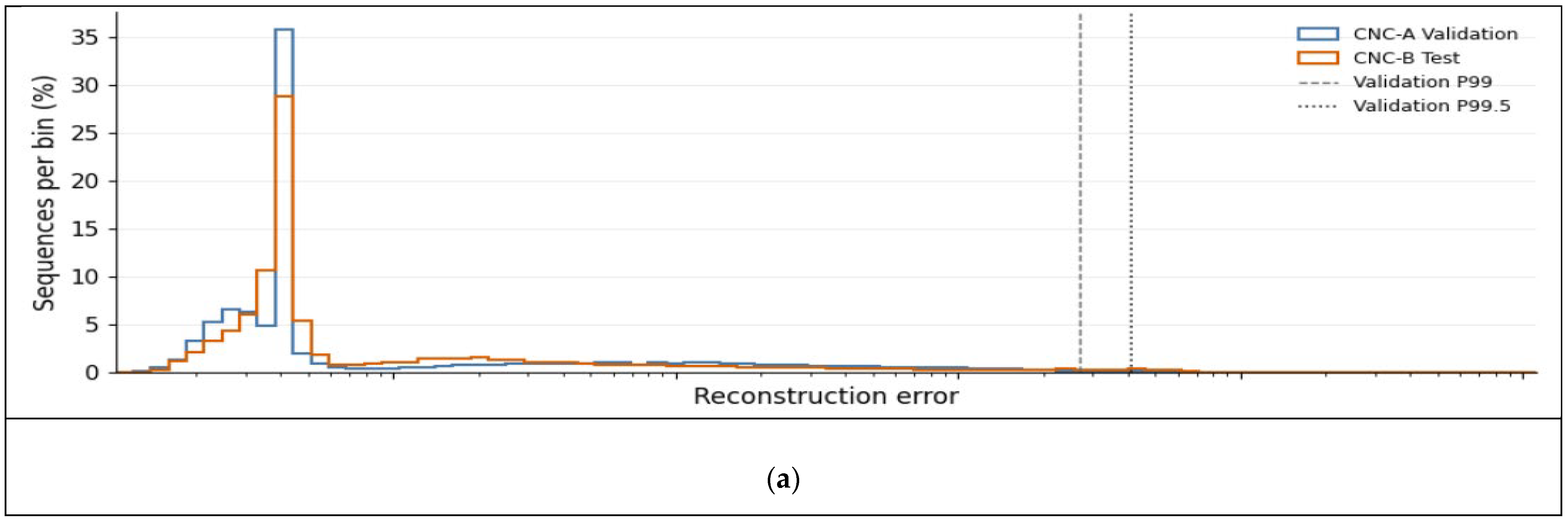
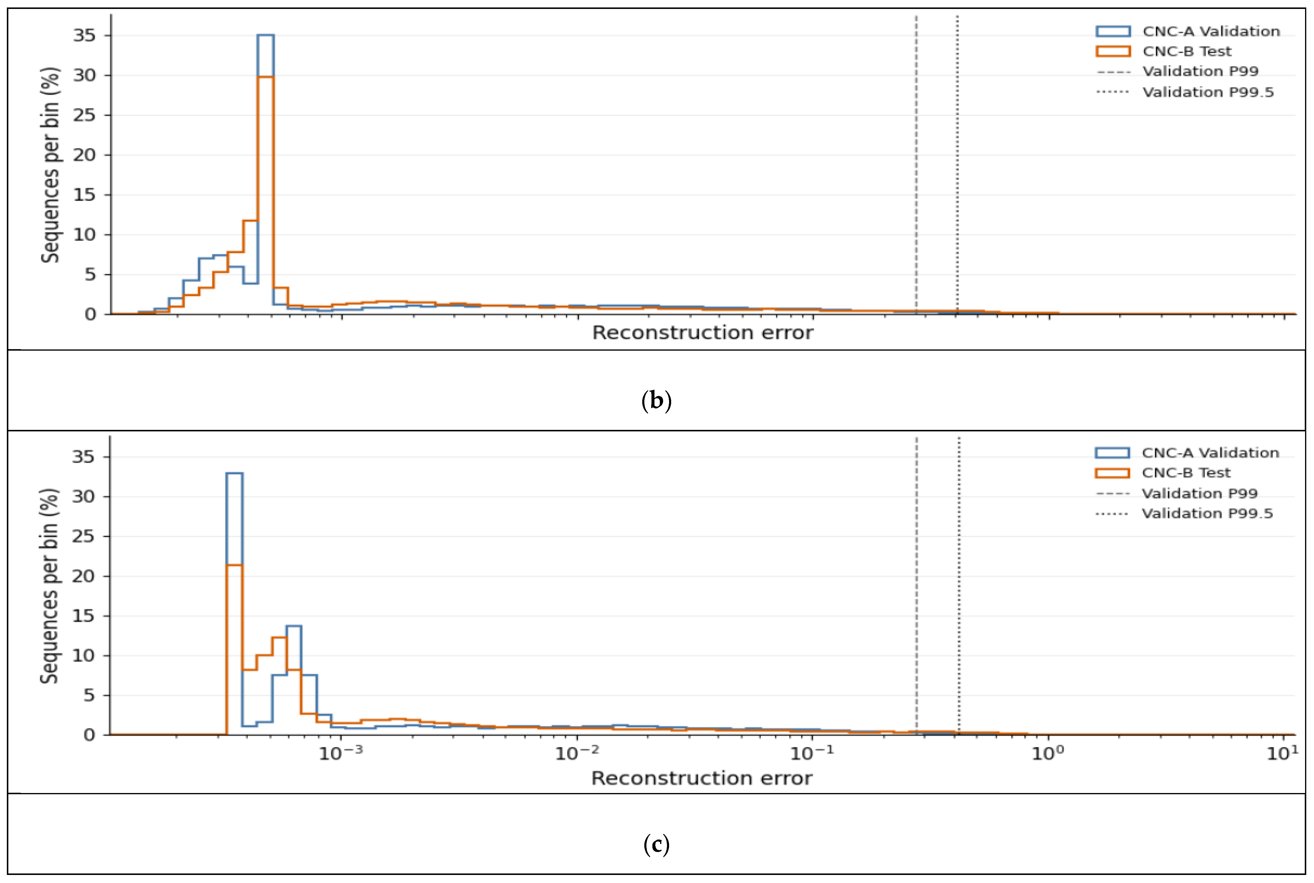
Comparison of the RE distributions showed that the test data had higher mean RE, standard deviation, and upper-percentile values than the validation data across all three random seeds. For seed 42, P99 was 0.271060 for the validation data and 0.445046 for the test data. For seeds 123 and 2024, P99 increased from 0.275027 and 0.277602 in the validation data to 0.428673 and 0.434724 in the test data, respectively. In contrast, the median values were similar between the two datasets. These results indicate that typical reconstruction error levels were comparable, whereas relatively larger reconstruction errors occurred in the upper tail of the test RE distribution.

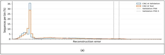
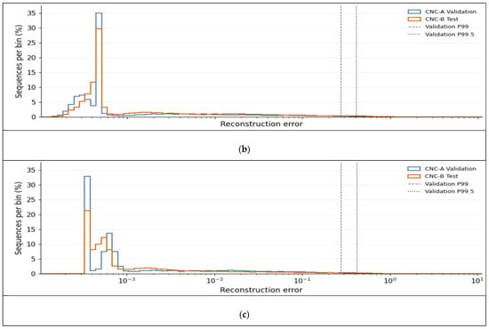
Figure 5 compares the RE distributions of the validation and test datasets. The P99 and P99.5 thresholds derived from the validation data for each model are also shown.

Figure 5. Comparison of reconstruction error distributions between CNC-A validation and CNC-B test datasets for random seeds (a) 42, (b) 123, and (c) 2024.

Test sequences were classified into three categories according to the statistical thresholds: RE ≤ P99, P99 < RE ≤ P99.5, and RE > P99.5. The validation thresholds corresponding to each model were applied, and mutually exclusive decision criteria were used to ensure that each sequence belonged to only one category. The number and proportion of sequences in each category are presented in Table 21.

Table 21. Number and proportion of CNC-B test sequences by RE threshold category.

Seed	RE ≤ P99	P99 < RE ≤ P99.5	RE > P99.5
42	28,345 (97.738%)	303 (1.045%)	353 (1.217%)
123	28,386 (97.879%)	298 (1.028%)	317 (1.093%)
2024	28,377 (97.848%)	315 (1.086%)	309 (1.065%)

The proportion of test sequences with RE at or below P99 ranged from 97.738% to 97.879%. The number of potential anomalies exceeding P99 was 656 (2.262%) for seed 42, 615 (2.121%) for seed 123, and 624 (2.152%) for seed 2024. Of these, 353 (1.217%), 317 (1.093%), and 309 (1.065%), respectively, exceeded P99.5. The counts of sequences exceeding P99 include those exceeding P99.5.

To assess agreement in the identification of potential anomalies across random seeds, the decisions of the three models were compared for the same test sequences. A sequence was classified as a potential anomaly when its RE exceeded the validation P99 threshold of the corresponding model. The number of models identifying each sequence as a potential anomaly was then counted, yielding values from 0 to 3. A count of 0 indicates that none of the models identified the sequence as a potential anomaly; counts of 1 and 2 indicate identification by one and two models, respectively; and a count of 3 indicates identification by all three models. The agreement in potential anomaly identification across the three random seeds is summarized in Table 22.

Table 22. Agreement in the identification of potential anomalies across random seeds.

Number of Seeds Identifying Anomaly Candidates	Sequence Count	Rate (%)
0	28,299	97.579
1	76	0.262
2	59	0.203
3	567	1.955
Total	29,001	100.000

These results demonstrate that the developed system can identify sequences requiring further examination by applying RE thresholds established using normal validation data to test data from a different CNC machine tool. In particular, sequences identified by all three models consistently exceeded the thresholds despite differences in random seed. These sequences can therefore be selected for subsequent examination of operating records and vibration patterns. The system can thus support on-site inspection by quantifying reconstruction discrepancies relative to normal operating patterns and identifying potential anomalies using statistical thresholds.

5. Conclusions

In this study, an LSTM autoencoder-based vibration anomaly detection system was developed for the servomotor driving the ball screw in a CNC machine tool. The system comprised data acquisition and storage using wireless vibration sensors, exclusion of data recorded during equipment inactivity, segmentation into continuous intervals, time series feature generation, model training, reconstruction error calculation, and identification of potential anomalies using statistical thresholds. This workflow transformed vibration data collected in the production environment into model inputs and identified sequences requiring further examination based on reconstruction discrepancies relative to normal operating patterns.

The input features were selected by progressively comparing the contributions of Moving Average, Standard Deviation, Slope, ΔRMS, and Growth Rate relative to Vibration RMS alone. In the F0–F13 comparison, F1 achieved the lowest mean MAE, whereas F4 achieved the lowest mean RMSE and the highest mean R². However, combining the two additional features or increasing the number of input features did not consistently improve upon these configurations. In the subsequent comparison of F0, F1, and F4 using the full training and validation datasets, F1 achieved the lowest mean MAE and RMSE of 0.061950 and 0.199993, respectively, and the highest mean R² of 0.816099. Its RMSE standard deviation of 0.001542 was also the lowest among the compared configurations. Accordingly, considering both reconstruction performance and variability across training runs, F1, comprising Vibration RMS and Moving Average, was selected as the final input configuration. Following comparisons of model architectures and loss configurations, Model C and the RMS loss configuration were adopted for the final model.

The final model was evaluated using normal operating data from CNC-B, which had not been used for training or model selection. The test dataset comprised 29,001 sequences generated from 165 continuous segments, with each sequence containing 60 time steps and two input features. The standardization parameters derived from the CNC-A training data were applied unchanged. Reconstruction results were obtained without further training or recalibration of the transformation parameters using the test data. Across the three random seeds, Vibration RMS R² was 0.938569 ± 0.000682 across all time steps and 0.931685 ± 0.005062 at the final time step. MAE and RMSE were higher at the final time step than across all time steps, and discrepancies between measured and reconstructed values were observed for some large vibration values and intervals exhibiting abrupt changes. These results indicate that, under the test conditions examined, the final model reproduced vibration patterns from a different CNC machine tool to a certain extent.

For the identification of potential anomalies, RE was defined as the mean squared error between the standardized input and reconstructed sequences. The median RE of the CNC-A normal validation data was defined as the Reference RE, and P99 and P99.5 were used as statistical screening thresholds. Across the three random seeds, the mean P99 and P99.5 thresholds were 0.274563 ± 0.003296 and 0.415222 ± 0.006584, respectively. When the thresholds for each model were applied to the CNC-B test data without adjustment, 2.121–2.262% of the sequences exceeded P99, and 1.065–1.217% exceeded P99.5. Although the median test RE was similar to that of the validation data, the mean and upper-percentile values were higher. This indicates that some test sequences exhibited larger reconstruction discrepancies than those observed in the normal validation data.

Comparison of the screening results across random seeds showed that 567 sequences exceeded P99 for all three models, accounting for 1.955% of the test sequences. A total of 28,299 sequences were not flagged by any model, and all three models agreed on whether a sequence was a potential anomaly for 99.534% of the test sequences. In contrast, decisions differed across seeds for 135 sequences. These results indicate consistency in the screening outcomes across model initializations under the test conditions examined. In particular, sequences identified by all three models can be selected for further examination of operating records and vibration patterns.

However, because the data contained no actual anomalies or faults, fault detection rates, missed detection rates, and performance in distinguishing fault types could not be evaluated. Reconstruction error can be influenced by operating conditions and differences in data distributions, as well as by equipment condition; a low reconstruction error therefore does not guarantee normal operation. Future work should validate the relationship between screening results and equipment condition using data with documented anomalies and maintenance histories and extend the evaluation to a wider range of CNC machines and operating conditions. Methods for grouping consecutively flagged sequences into intervals and analyzing the duration and recurrence of threshold exceedances should also be examined. As a tool for quantifying reconstruction discrepancies in vibration data and identifying targets for further examination, the developed system can support condition monitoring and on-site inspection of CNC equipment.

References

- Xu, X. Machine Tool 4.0 for the new era of manufacturing. Int. J. Adv. Manuf. Technol. 2017, 92, 1893–1900. [Google Scholar] [CrossRef] [Scilit]
- Li, K.; Qiu, C.; Li, C.; He, S.; Li, B.; Luo, B.; Liu, H. Vibration-based health monitoring of ball screw in changing operational conditions. J. Manuf. Process. 2020, 53, 55–68. [Google Scholar] [CrossRef] [Scilit]
- Teti, R.; Jemielniak, K.; O’Donnell, G.; Dornfeld, D. Advanced monitoring of machining operations. CIRP Ann. 2010, 59, 717–739. [Google Scholar] [CrossRef] [Scilit]
- Jardine, A.K.S.; Lin, D.; Banjevic, D. A review on machinery diagnostics and prognostics implementing condition-based maintenance. Mech. Syst. Signal Process. 2006, 20, 1483–1510. [Google Scholar] [CrossRef] [Scilit]
- Carvalho, T.P.; Soares, F.A.A.M.N.; Vita, R.; Francisco, R.P.; Basto, J.P.; Alcalá, S.G.S. A systematic literature review of machine learning methods applied to predictive maintenance. Comput. Ind. Eng. 2019, 137, 106024. [Google Scholar] [CrossRef] [Scilit]
- Zonta, T.; da Costa, C.A.; da Rosa Righi, R.; de Lima, M.J.; da Trindade, E.S.; Li, G.P. Predictive maintenance in the Industry 4.0: A systematic literature review. Comput. Ind. Eng. 2020, 150, 106889. [Google Scholar] [CrossRef] [Scilit]
- Yang, R.; Huang, M.; Lu, Q.; Zhong, M. Rotating machinery fault diagnosis using long-short-term memory recurrent neural network. IFAC—PapersOnLine 2018, 51, 228–232. [Google Scholar] [CrossRef] [Scilit]
- Çekik, R.; Turan, A. Deep learning for anomaly detection in CNC machine vibration data: A RoughLSTM-based approach. Appl. Sci. 2025, 15, 3179. [Google Scholar] [CrossRef] [Scilit]
- Kim, J.; Lee, H.; Jeon, J.W.; Kim, J.M.; Lee, H.U.; Kim, S. Stacked auto-encoder based CNC tool diagnosis using discrete wavelet transform feature extraction. Processes 2020, 8, 456. [Google Scholar] [CrossRef] [Scilit]
- Dou, J.; Xu, C.; Jiao, S.; Li, B.; Zhang, J.; Xu, X. An unsupervised online monitoring method for tool wear using a sparse auto-encoder. Int. J. Adv. Manuf. Technol. 2020, 106, 2493–2507. [Google Scholar] [CrossRef] [Scilit]
- Yan, S.; Shao, H.; Xiao, Y.; Liu, B.; Wan, J. Hybrid robust convolutional Autoencoder for unsupervised anomaly detection of machine tools under noises. Robot. Comput. Integr. Manuf. 2023, 79, 102441. [Google Scholar] [CrossRef] [Scilit]
- Oshida, T.; Murakoshi, T.; Zhou, L.; Ojima, H.; Kaneko, K.; Onuki, T.; Shimizu, J. Development and implementation of real-time anomaly detection on tool wear based on stacked LSTM encoder-decoder model. Int. J. Adv. Manuf. Technol. 2023, 127, 263–278. [Google Scholar] [CrossRef] [Scilit]
- Demetgul, M.; Zheng, Q.; Tansel, I.N.; Fleischer, J. Monitoring the misalignment of machine tools with Autoencoders after they are trained with transfer learning data. Int. J. Adv. Manuf. Technol. 2023, 128, 3357–3373. [Google Scholar] [CrossRef] [Scilit]
- Yao, K.-C.; Chen, D.-C.; Pan, C.-H.; Lin, C.-L. The development trends of computer numerical control (CNC) machine tool technology. Mathematics 2024, 12, 1923. [Google Scholar] [CrossRef] [Scilit]
- Yu, Z.; Liu, N.; Wang, K.; Sun, X.; Sheng, X. Design of fuzzy PID controller based on sparse fuzzy rule base for CNC machine tools. Machines 2023, 11, 81. [Google Scholar] [CrossRef] [Scilit]
- Zhang, H.; Zha, J.; Du, C.; Liu, H.; Li, Y.; Lv, D. Variable-coefficient dynamic modeling method for a ball screw feed system in the no-extra-load running state. Processes 2023, 11, 793. [Google Scholar] [CrossRef] [Scilit]
- Liu, H.; Guo, Y.; Liu, J.; Niu, W. Dynamic error compensation for ball screw feed drive systems based on prediction model. Machines 2025, 13, 433. [Google Scholar] [CrossRef] [Scilit]
- Wu, Q.; Niu, J.; Wang, X. Study on life prediction method of ball screw base on constructed degradation feature and IGWO-BiLSTM. Actuators 2023, 12, 236. [Google Scholar] [CrossRef] [Scilit]
- Zaidi, S.H.H.; Shenfield, A.; Zhang, H.; Ikpehai, A. A systematic review of anomaly and fault detection using machine learning for industrial machinery. Algorithms 2026, 19, 108. [Google Scholar] [CrossRef] [Scilit]
- Givnan, S.; Chalmers, C.; Fergus, P.; Ortega-Martorell, S.; Whalley, T. Anomaly detection using Autoencoder reconstruction upon industrial motors. Sensors 2022, 22, 3166. [Google Scholar] [CrossRef] [Scilit]
- Pearson, R.K.; Neuvo, Y.; Astola, J.; Gabbouj, M. Generalized Hampel Filters. EURASIP J. Adv. Signal Process. 2016, 2016, 87. [Google Scholar] [CrossRef] [Scilit]
- Maleki, S.; Maleki, S.; Jennings, N.R. Unsupervised anomaly detection with LSTM Autoencoders using statistical data-filtering. Appl. Soft Comput. 2021, 108, 107443. [Google Scholar] [CrossRef] [Scilit]
- Wei, Y.; Jang-Jaccard, J.; Xu, W.; Sabrina, F.; Camtepe, S.; Boulic, M. LSTM-Autoencoder-based anomaly detection for indoor air quality time-series data. IEEE Sens. J. 2023, 23, 3787–3800. [Google Scholar] [CrossRef] [Scilit]
- Lee, Y.; Park, C.; Kim, N.; Ahn, J.; Jeong, J. LSTM-Autoencoder based anomaly detection using vibration data of wind turbines. Sensors 2024, 24, 2833. [Google Scholar] [CrossRef] [Scilit]
Disclaimer/Publisher’s Note: The statements, opinions and data contained in all publications are solely those of the individual author(s) and contributor(s) and not of MDPI and/or the editor(s). MDPI and/or the editor(s) disclaim responsibility for any injury to people or property resulting from any ideas, methods, instructions or products referred to in the content. |
© 2026 by the authors. Licensee MDPI, Basel, Switzerland. This article is an open access article distributed under the terms and conditions of the Creative Commons Attribution (CC BY) license.