


Abstract
This study evaluates leakage-controlled feature fusion for five shafting-adjustment tasks and one bevel-gear contact-pattern task on a synthetic benchmark. The complete TransXGB procedure combines fold-standardized raw inputs, out-of-fold Transformer latents, and out-of-fold XGBoost leaf features. Ten methods were evaluated on identical repeated outer folds; the prespecified primary criterion was the six-task equal-weight mean standardized MAE across the pooled S0, S1, and S2 scenarios. Ridge achieved a slightly lower primary error than full TransXGB (0.211481 versus 0.211622), and inner selection over five Ridge penalties produced the same ordering (0.211430 versus 0.211622). In S1 and S2, TransXGB errors were 0.53% and 1.99% lower than prespecified Ridge, but both descriptive task-resampling intervals crossed zero. These scenarios were deliberately constructed with smooth and threshold nonlinearities, so the differences do not establish a general nonlinear advantage. Complete same-batch ablation outputs show that fixed inclusion of the XGBoost leaf branch did not yield a net error reduction in these six tasks, while raw-plus-Transformer was lowest in five tasks and Transformer removal worsened both pump tasks in all five folds. The leaf branch remains a leakage-controlled test of complementary tree-partition information; its result favors task-selective rather than fixed fusion. The benchmark does not demonstrate aggregate superiority or production accuracy.
1. Introduction
Dimensional variation propagates through mechanical transmission assemblies and affects shim selection, axial positioning, and bevel-gear contact. Classical dimensional chains remain the preferred transparent tool when signed closure equations, nominal dimensions, tolerance allocations, and deformation assumptions are available. Data-driven methods are attractive when interactions are nonlinear or incomplete, but their practical value depends as much on validation design as on nominal prediction error [1,2,3,4,5,6].
Recent work has applied neural surrogates, digital twins, multi-sensor learning, and Transformers to assembly-accuracy prediction [2,3,4,5,6,7]. Transformer attention can contextualize parameter interactions, whereas gradient-boosted trees can partition threshold-like tabular behavior [8,9,10,11]. Their fusion is therefore plausible, but three gaps remain. First, a whole input vector represented as one token yields a 1 × 1 attention matrix and cannot express attention among parameters. Second, target-dependent leaf indices can create optimistic stacking if a fusion model is trained on representations generated in sample. Third, comparison on a test set that has influenced architecture or hyperparameter selection is not independent, irrespective of whether the rows are later described as locked.
These concerns are especially important when the numerical tables are synthetic. Normally distributed tolerance-like draws can support controlled algorithm stress testing, but they are not production measurements and do not establish process capability, measurement validity, or cross-batch transfer [12,13,14]. Increasing the number of draws reduces Monte Carlo error only for the specified generator; it does not create additional physical evidence.
The evidence boundary is therefore methodological. Synthetic tolerance-like draws can test whether preprocessing, representation learning, and fusion are isolated within validation folds, but they cannot establish process capability, measurement validity, or transfer to a later manufacturing batch.
Accordingly, this study has four objectives: (1) define the six tasks and disclose which data-generation details are known and unknown; (2) implement parameter-level Transformer tokens and out-of-fold feature generation; (3) evaluate the complete leakage-controlled fusion procedure and reference methods using one prespecified primary criterion, with all scenario-, task-, target-, contact-exclusion, learning-curve, and ablation views labeled secondary or exploratory; and (4) identify negative findings and the evidence required before any engineering deployment claim can be tested.
2. Materials and Methods
2.1. Mechanical Tasks and Data Identity
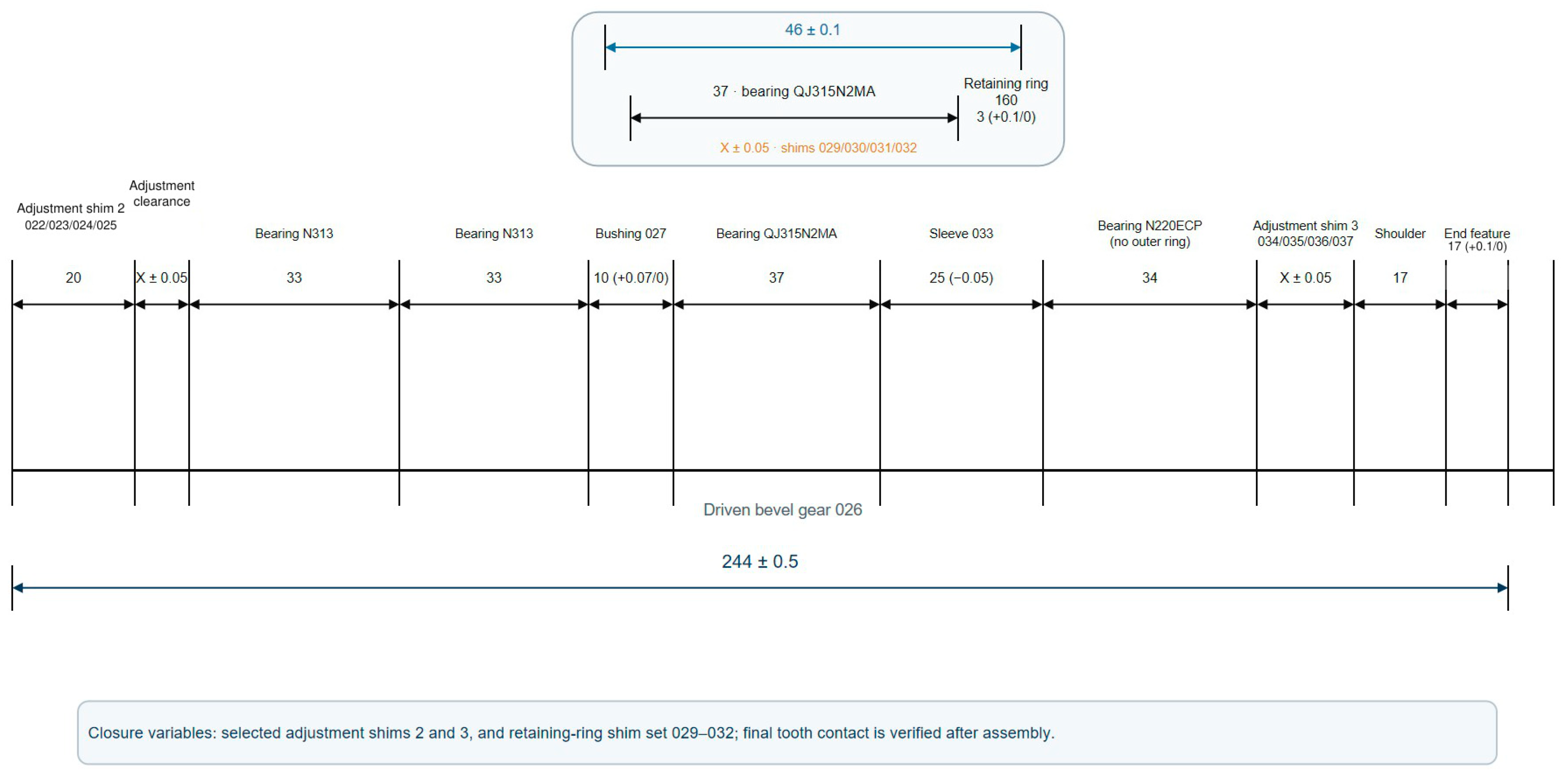
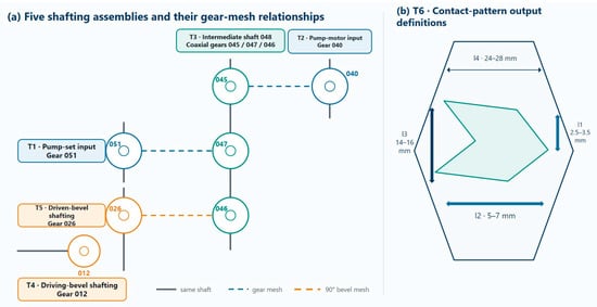
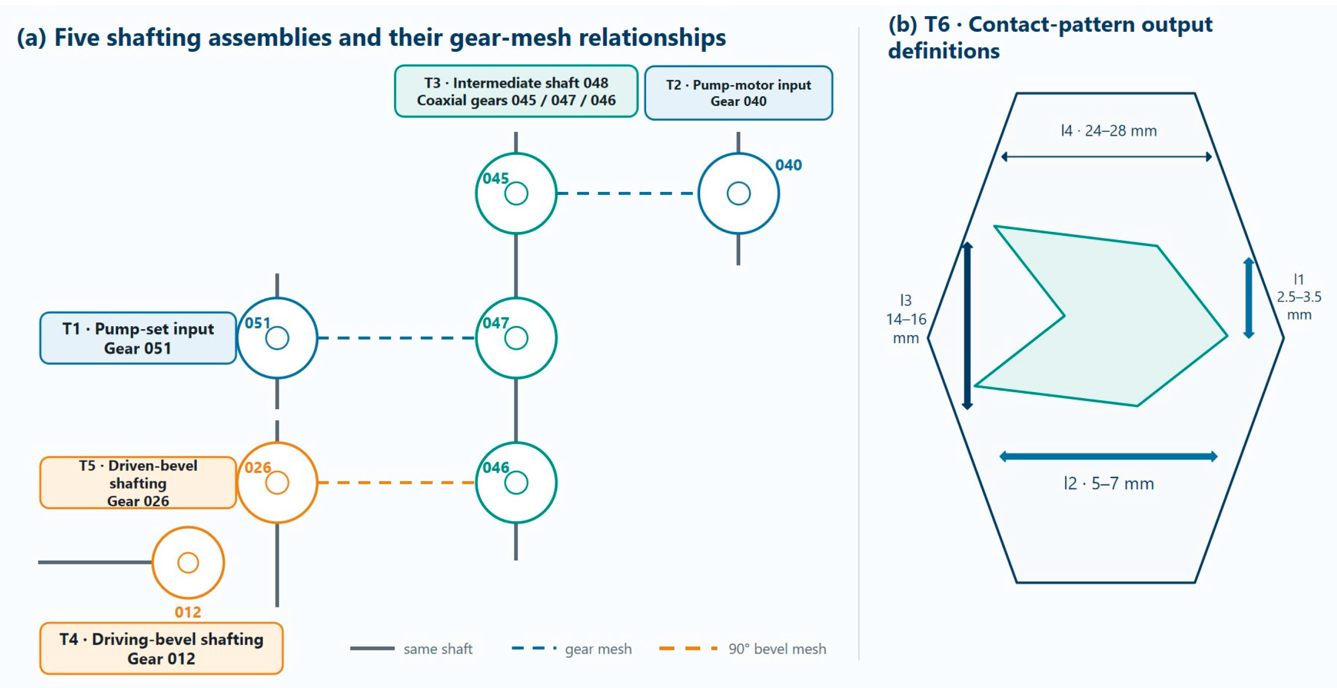
The front-transmission system is represented by five shafting-adjustment tasks and one bevel-gear contact-pattern task (Figure 1). Figure 1 is a task-location schematic rather than a manufacturing drawing. The shafting outputs are sleeve or shim dimensions; the contact outputs are four functional dimensions, l1–l4. Assembly-error and contact behavior in bevel gears motivate the separate contact task [15]. Five axial dimensional-chain schematics redrawn from the available assembly instructions are provided in Figure A1, Figure A2, Figure A3, Figure A4 and Figure A5 for the pump-motor input, pump-set input, intermediate-wheel, driving-bevel, and driven-bevel shafting systems. They identify the recorded component stacks, datums, closure dimensions, and adjustment variables, but are not treated as a numerical worst-case or statistical tolerance-chain baseline because the archive does not contain complete signed closure equations and all drawing-level tolerance allocations. Table 1 defines the notation, and Table A1 lists the input and output schemas.
Figure 1.
Vector schematic of the six prediction tasks: (a) five shafting locations and (b) four bevel-gear contact-pattern dimensions. The drawing defines prediction locations only and is not used as a dimensional-chain model. T1–T6 identify the tasks; three-digit numbers are component identifiers with leading zeros. Colors distinguish task groups; line styles are defined in the legend.
Table 1.
Symbols and scenario notation.
Data Composition, File Structure, and Scenario Coding
The submitted benchmark contains 5103 synthetic rows and exactly three consecutively numbered scenarios: S0_existing, S1_smooth, and S2_mixed. No standalone threshold-only or high-noise scenario is included in the manuscript results or the submitted data package. Pump-set, intermediate-wheel, driving-bevel, and driven-bevel shafting each contain 900 rows (300 per scenario); pump-motor shafting contains 903 rows (301 per scenario); and contact-pattern prediction contains 600 rows (200 per scenario). Thus, every task is exactly balanced across S0/S1/S2 before cross-validation (Table 2).
Table 2.
Task-wise input/output dimensions, pooled sample counts, and canonical scenario balance.
The project archive also contained 40 measured assembly records, approximately 20% of which showed evident entry errors or incomplete fields. Those records were used only to identify task definitions and plausible engineering ranges. No measured record was included as a modeling row, and no row-level linkage exists between the 40 records and the six legacy modeling workbooks. Because the assemblies had already been completed, additional prospective records and repeat measurements could not be collected for this revision.
Each task folder contains augmented_train.csv, augmented_validation.csv, and component_audit_not_for_modeling.csv. The first two files contain synthetic_id, generator_seed, source_kind, scenario, the task-specific dimensional inputs, and the corresponding output columns. The audit file stores standardized linear, smooth, threshold, and noise components solely to verify the generator; these component labels are never supplied to a model as inputs or supervision. The former train and validation tables contribute 600 + 300 rows for each 900-row task, 603 + 300 for pump-motor shafting, and 300 + 300 for contact pattern. Because those legacy roles had influenced prior development, they are pooled before the repeated nested-CV split and are not called an independent test set. Fold-local preprocessing and model selection are then applied to the pooled rows.
S0 consists of input–output rows copied unchanged from six legacy modeling workbooks. Project provenance identifies those workbooks as normally generated rather than measured production data, but the original S0 generator code, target equation, random seed, and noise specification were not archived. The S0 response therefore cannot be classified retrospectively as deterministic or stochastic. S1 uses newly drawn correlated normal inputs and a Ridge-estimated linear response plus fixed smooth pairwise, quadratic, and sinusoidal terms. S2 uses the same input construction and adds two threshold-switching terms. Independent Gaussian noise with standard deviation 0.035 in standardized target units is added only to the newly generated S1 and S2 rows.
2.2. Synthetic Training-Data Construction
For S1 and S2, the legacy development workbooks supplied the input mean, marginal standard deviation, and correlation matrix. The correlation matrix was shrunk 15% toward identity, standardized multivariate-normal draws were clipped to [−3, 3], and values were transformed back to engineering units. This procedure did not regenerate or alter S0.
For the newly generated S1 and S2 rows, a Ridge model fitted to standardized legacy inputs and outputs supplied a linear reference response. S1 added fixed smooth interaction terms; S2 added the same smooth terms and two threshold effects. The archived generator records every newly generated component. No corresponding decomposition is available for S0 because its original target-generation rule is unknown. Table 3 summarizes the scenarios.
y* = ylinear + IS1,S2ϕs(z) + IS2ϕt(z) + ε, ε∼(0,0.0352).
ϕt(z) = 0.10I(zg > 0.7) − 0.08I(zb < −0.5, zg > 0).
Table 3.
Prespecified synthetic scenarios.
This construction was adopted because the archive of 40 real assembly records was too small for reliable model development, approximately one fifth contained evident record errors, and the completed assembly campaign could not be prospectively expanded. Correlated normal draws provide a tolerance-like numerical cloud, smooth interactions can reward contextual representations, and threshold terms can reward partition-based learners [8,9,16,17]. Nevertheless, the rule is not a material law, a signed dimensional chain, or a calibrated manufacturing process. The generator seed, row identifier, scenario label, executable rule, and SHA-256 hashes are archived. No generated row is relabeled as a measured part, and the increased row count must not be interpreted as additional physical evidence.
2.3. Parameter-Token Transformer
Unlike the earlier single-token formulation, each standardized scalar parameter is mapped to its own token. A learned feature-identity embedding distinguishes columns without treating spreadsheet order as a physical sequence:
The encoder contains one layer, four attention heads, model width 16, a 32-unit GELU feed-forward block, dropout 0.15, residual connections, and LayerNorm. For head h,
Accordingly, Ah has dimensions d × d rather than 1 × 1 and can contextualize pairs of assembly parameters. Mean pooling produces a 16-dimensional latent representation. A conventional MLP and a two-layer MLP matched as closely as possible to the Transformer trainable-parameter count are evaluated to distinguish attention effects from capacity effects.
2.4. XGBoost Leaf Representation and OOF Fusion
For each target, XGBoost (version 3.4.1) fits 80 regression trees with maximum depth 2, learning rate 0.04, minimum child weight 3, row subsampling 0.85, column subsampling 0.90, L2 regularization 3.0, and L1 regularization 0.01 [8]. Terminal-leaf identities are one-hot-encoded in the fitting fold and reduced to 8 or 16 dimensions by fold-local TruncatedSVD (scikit-learn 1.8.0). The numerical XGBoost prediction is never used as a fusion input.
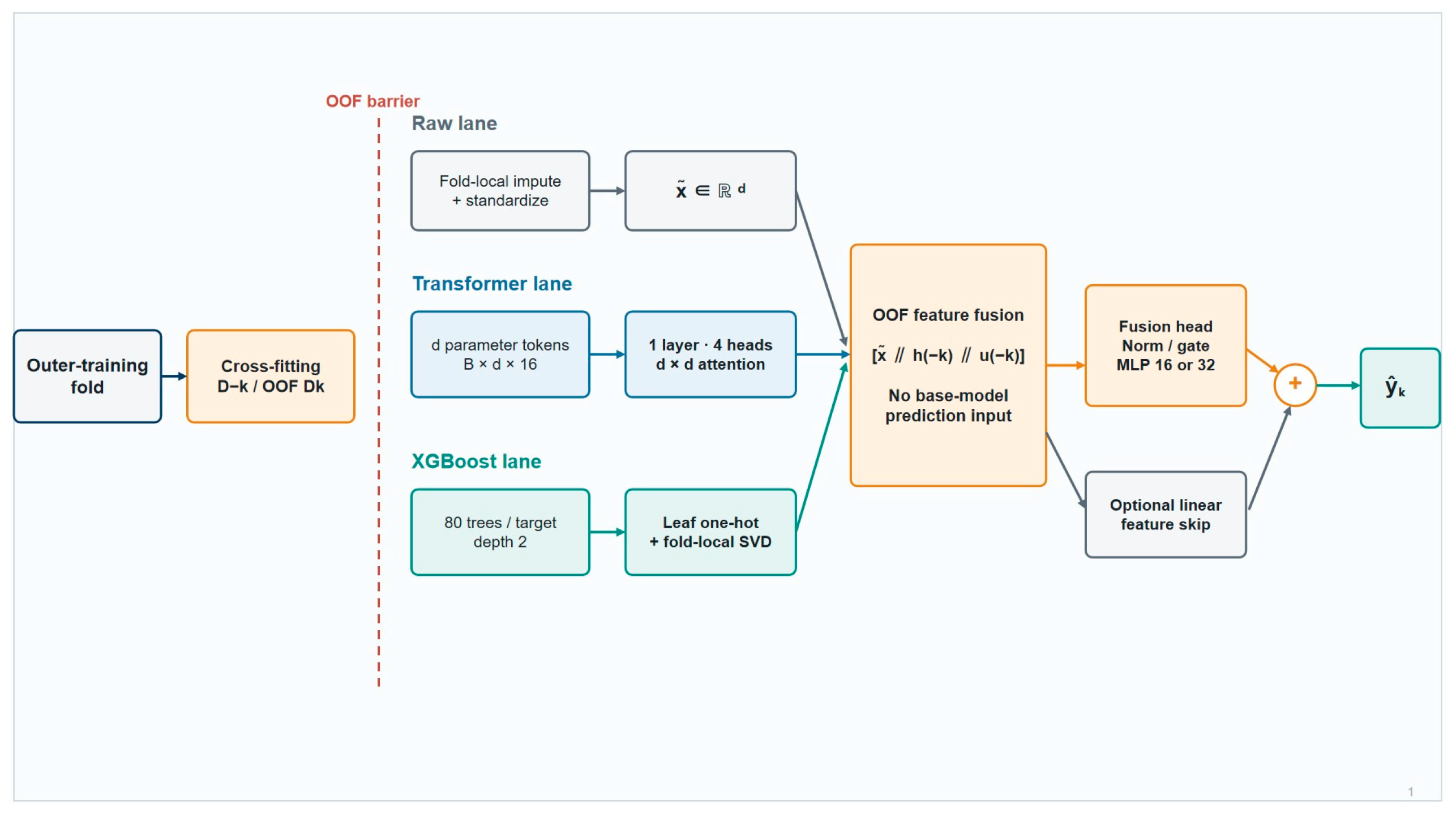
For each cross-fit split k inside an outer-training fold, the Transformer and XGBoost models are trained on D−k and applied to Dk. The fusion head is trained only on Dk labels paired with representations from models that did not train on those rows. Fold-standardized raw parameters are included as a transparent identity path:
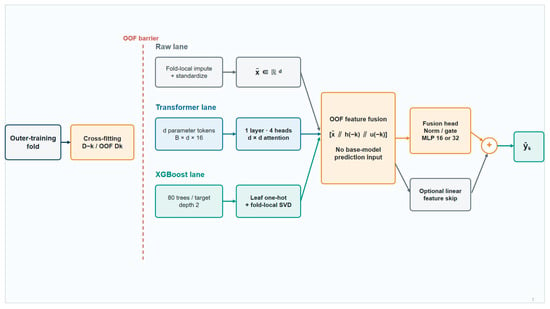
The fold-specific fusion head uses a 16- or 32-unit MLP, Huber or MSE loss, optional branch normalization, and an optional linear feature skip initialized by Ridge. These are feature-level operations; Ridge, Transformer, and XGBoost predictions are not stacked or averaged. Figure 2 separates the three feature lanes and the OOF barrier.
Figure 2.
Leakage-controlled TransXGB architecture. Every fusion-training label is paired with raw, Transformer-latent, and XGBoost-leaf features generated within the permitted outer-training and cross-fitting boundaries; base-model predictions are not fusion inputs.
2.5. Repeated Nested Cross-Validation
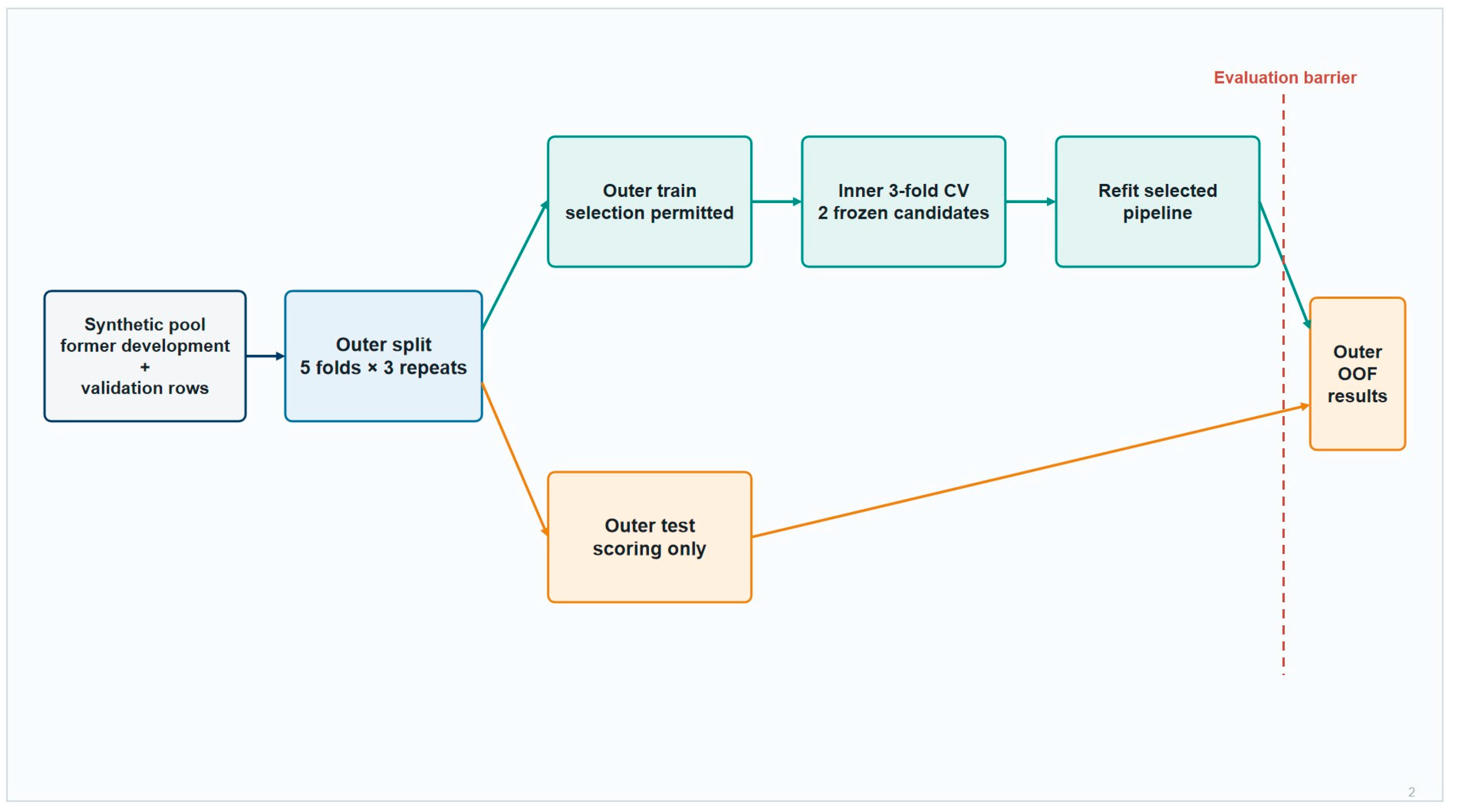
The former held-out test/validation set had been used during prior architecture comparison and therefore ceased to be independent. The present analysis pools the former development and validation rows and evaluates the complete selection procedure by repeated nested cross-validation. Identical outer folds are used for every method. TransXGB selects between two frozen candidates inside each outer-training fold. Reference models use prespecified fixed configurations in the primary benchmark; because Ridge is the aggregate leader and principal comparator, a requested model-selection sensitivity analysis additionally selects alpha from {0.01, 0.1, 1, 10, 100} by the same three-fold inner-CV objective and outer folds. Figure 3 and Table 4 summarize the protocol.
Figure 3.
Repeated nested-CV protocol. The inner loop selects a prespecified TransXGB candidate using only the outer-training fold; the outer test fold is accessed once for scoring, and the process yields 15 outer-OOF predictions per task.
Table 4.
Leak-controlled training and validation protocol.
Candidate A is the task-specific configuration frozen before the nested rerun. Candidate B is generated mechanically from A by swapping leaf-compression dimension 8 and 16, swapping fusion width 16 and 32, toggling branch normalization, disabling feature gating, and using a shared output head; all other task-specific settings are inherited. Both candidates use the same parameter-token encoder, raw-input lane, OOF Transformer and leaf features, optimizer, and data boundary. The inner objective is equal-target standardized MAE. Appendix Table A2 lists the exact task-level candidates and selection counts; L/W/N/H denotes leaf dimension, fusion width, normalization (1 = yes), and head type (S = shared; P = per-target). No candidate was changed after outer-OOF inspection.
2.6. Reference Models and Metrics
Figure A1, Figure A2, Figure A3, Figure A4 and Figure A5 provide the five available engineering dimensional-chain schematics and identify their component stacks and adjustment variables. A numerical dimensional-chain baseline could not be reconstructed because the archive lacks complete signed closure equations, deformation terms, and drawing-level tolerance allocations. The primary reference models (Table 5) therefore use frozen specifications on the same outer folds. The nested Ridge sensitivity analysis tests whether the main comparison depends on its fixed alpha; the remaining fixed baselines are secondary references rather than compute-matched claims of model-class superiority.
Table 5.
Models evaluated on identical outer folds.
MAE, RMSE, MSE, and R2 are calculated separately for each target. Cross-task comparisons use standardized MAE, with the target standard deviation estimated only from the corresponding outer-training fold. Contact-pattern results additionally use NMAE and NRMSE with functional spans of 1, 2, 2, and 4 mm:
The prespecified primary evaluation criterion is the six-task equal-weight mean standardized MAE across pooled S0, S1, and S2 outer-OOF predictions. This criterion gives each task family equal weight regardless of row or target count. Scenario-specific values, task and target rankings, the analysis excluding contact outputs, learning curves, component ablation, and tuned-Ridge comparison are secondary or exploratory. For the paired TransXGB-Ridge difference, the six task-family means were resampled with replacement 20,000 times; the resulting 2.5th and 97.5th percentiles are descriptive task-mix sensitivity intervals, not population confidence intervals. Appendix Table A3 reports every paired difference by task, scenario, and repeat.
3. Results
3.1. Method-Level Repeated Outer-OOF Results
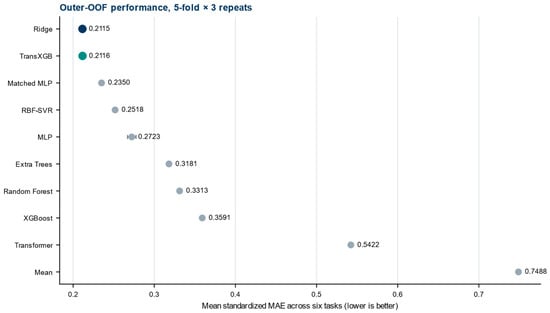
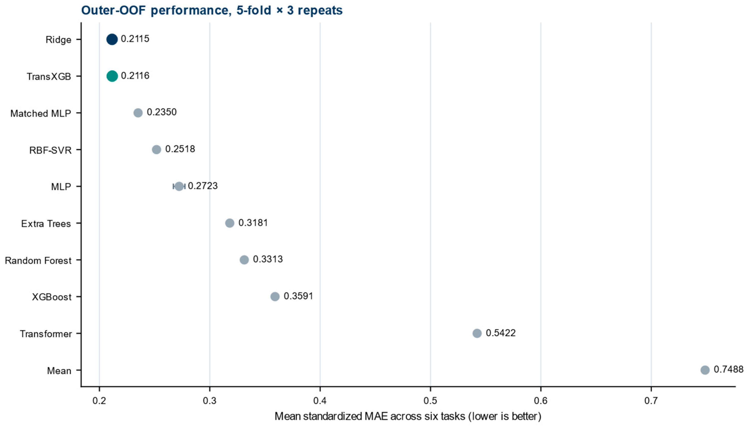
On the primary criterion (Table 6; Figure 4), prespecified Ridge ranked first at 0.211481 and full TransXGB ranked second at 0.211622. The paired difference (TransXGB minus Ridge) was +0.000141, or 0.07% relative to Ridge, with a descriptive 95% task-resampling interval of −0.003913 to +0.004447. The repeat-specific differences were −0.000059, −0.000717, and +0.001200. In the matched model-selection sensitivity analysis, inner-selected Ridge achieved 0.211430, so the primary ordering was unchanged, and the TransXGB disadvantage increased slightly to 0.000192 (0.09%). The aggregate evidence does not support TransXGB superiority.
Table 6.
Six-task method-level performance under repeated nested cross-validation.
Figure 4.
Six-task mean standardized MAE from outer-OOF predictions. Error bars show the standard deviation across three outer repeats; lower values are better.
3.2. Task- and Target-Level Performance
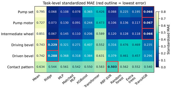
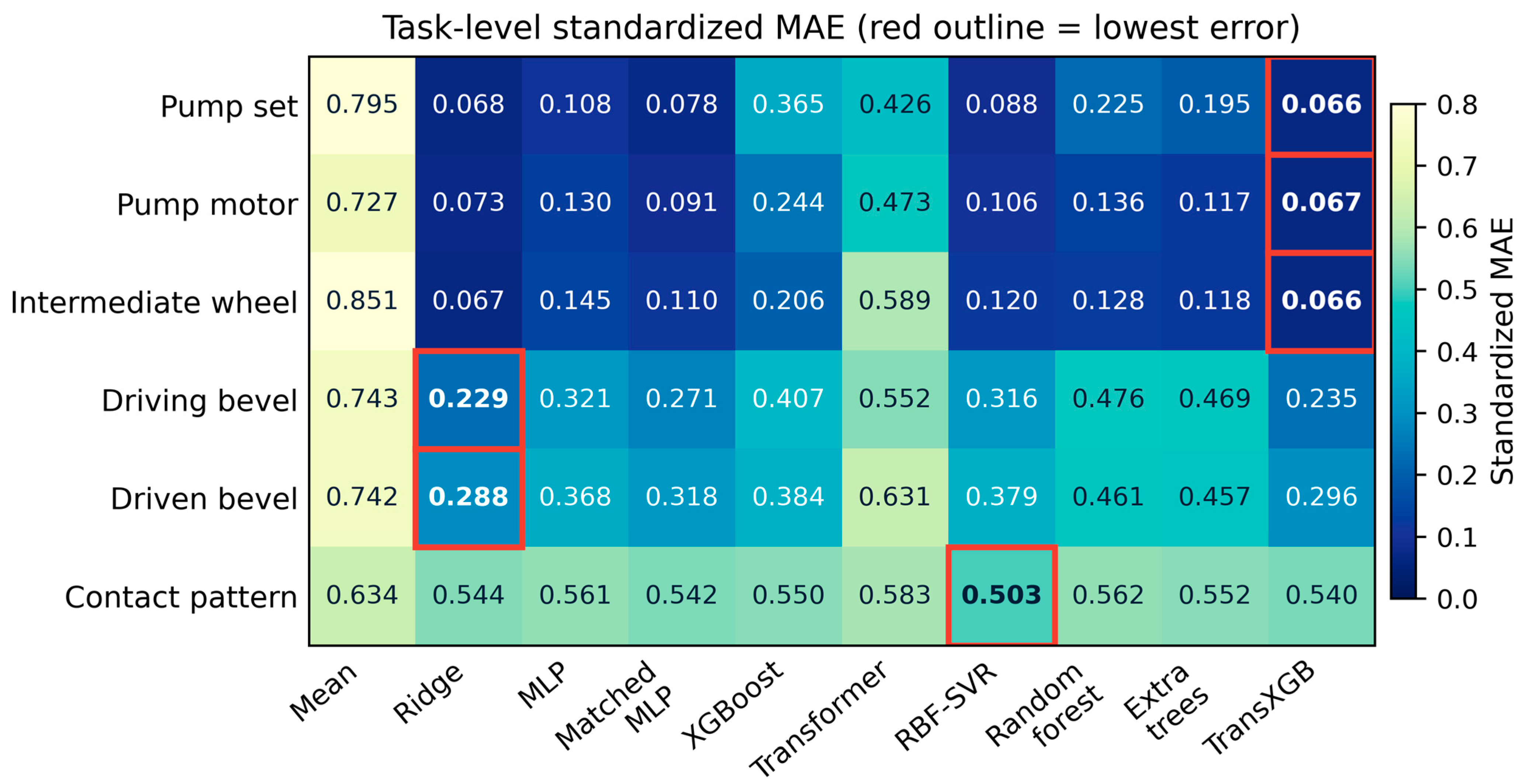
In the secondary task-level view (Table 7; Figure 5), full TransXGB ranked first for pump-set, pump-motor, and intermediate-wheel shafting; Ridge ranked first for both bevel-shafting tasks; and RBF-SVR ranked first for contact pattern. These heterogeneous task rankings do not replace the primary equal-task aggregate, on which Ridge remained marginally better.
Table 7.
Combined-view task-family standardized MAE.
Figure 5.
Task-level standardized MAE for all ten methods. Red outlines identify the lowest error in each task.
In the secondary nonlinear-scenario view, full TransXGB achieved equal-task standardized MAE values of 0.103120 in S1 and 0.106238 in S2, compared with 0.103666 and 0.108390 for prespecified Ridge. The observed reductions were 0.53% and 1.99%; paired task-resampling intervals (−0.006642 to +0.005563 in S1 and −0.007366 to +0.003210 in S2) crossed zero. Inner-selected Ridge yielded 0.103677 and 0.108463, corresponding to similarly small TransXGB reductions of 0.54% and 2.05%. Because S1 and S2 were deliberately constructed with smooth and threshold terms, these mechanism-specific point differences do not establish a reproducible or general nonlinear advantage.
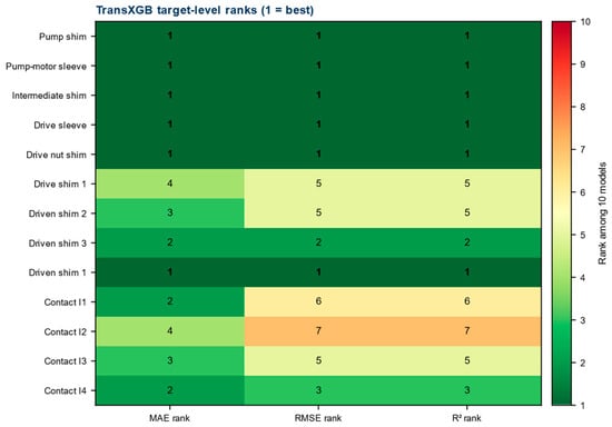
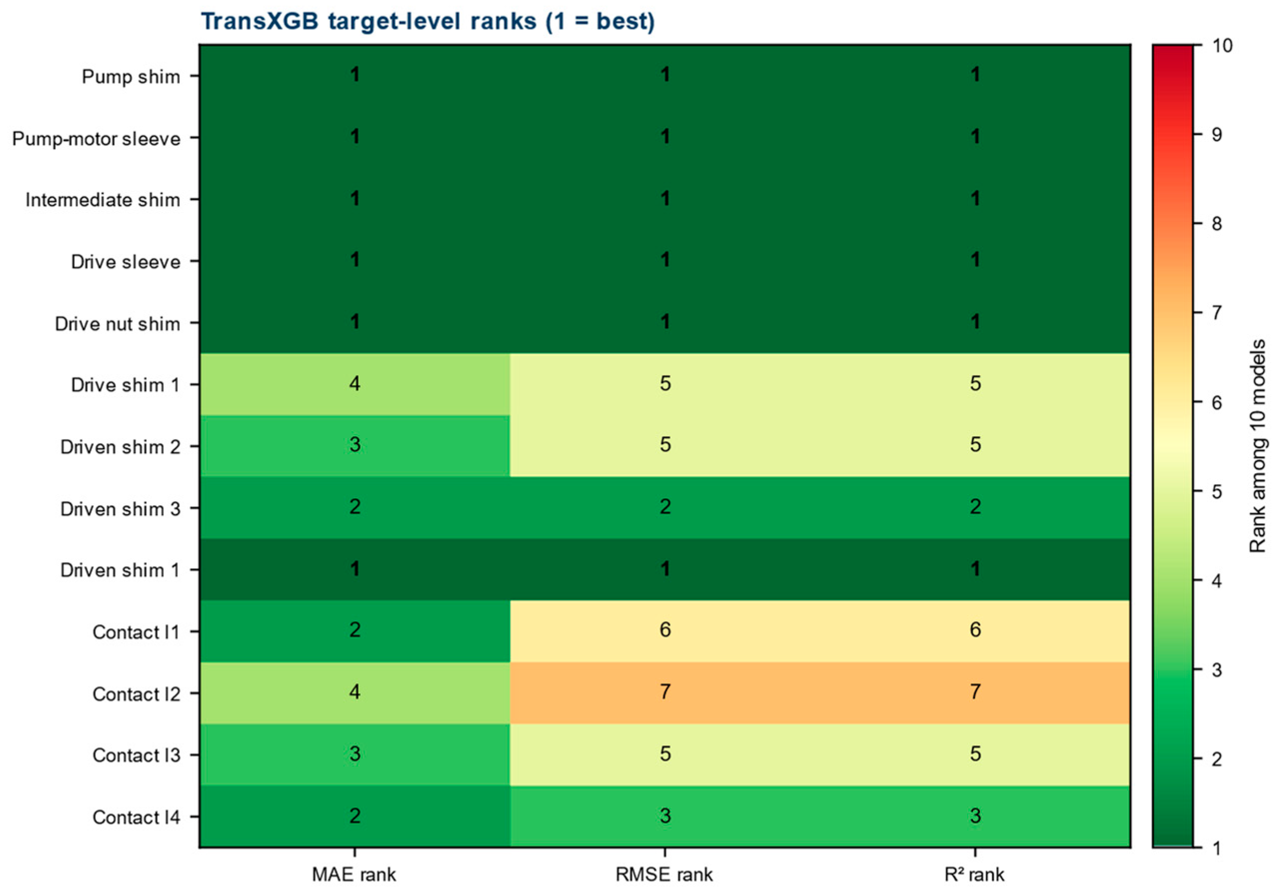
The target-ranking and contact-exclusion summaries (Table 8; Figure 6) are exploratory. After excluding the four failed contact outputs, full TransXGB ranked first for six of nine shafting targets under MAE, RMSE, and R2. This selected view does not alter the primary aggregate result, the intervals crossing zero, or the negative leaf-branch ablation.
Table 8.
Combined-view TransXGB target-level results.
Figure 6.
TransXGB rank by MAE, RMSE, and R2 for each target under repeated outer-OOF evaluation.
3.3. Contact-Pattern Boundary Case and Normalized Metrics
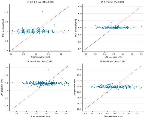
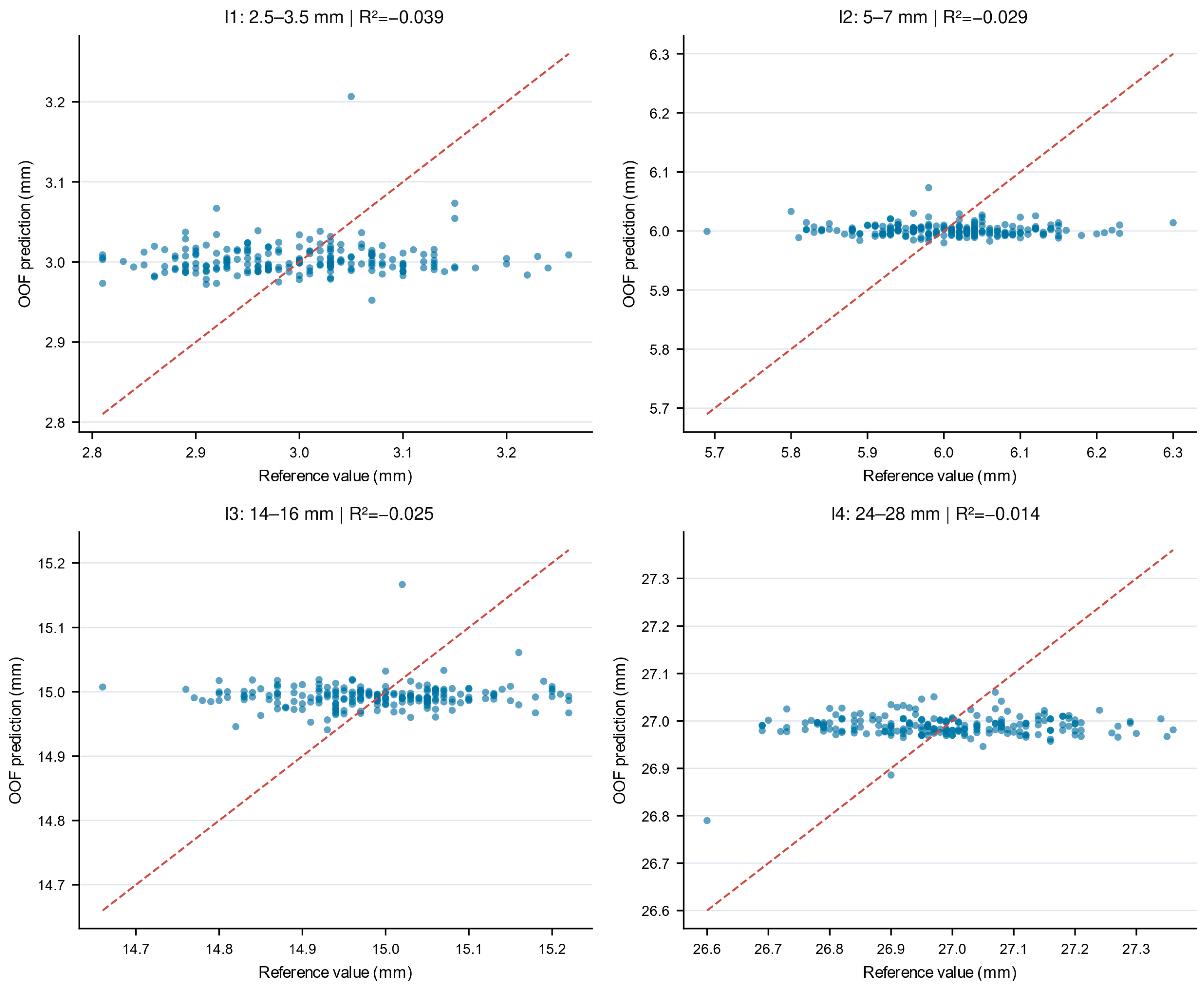
The four S0 R2 values (Table 9; Figure 7) ranged from −0.0391 to −0.0140 and were all below the training-mean reference. Thus, the model did not achieve reliable individual-level discrimination for these legacy synthetic contact rows. Because the original S0 target rule is unavailable and no measured contact assemblies were modeled, the failure cannot be attributed to a specific physical cause. The three retained inputs omit tooth-flank geometry, surface state, load, inspection conditions, material, heat treatment, machining variation, and measurement-system information that a future production study would need to collect. Negative R2 is reported as a boundary result for this benchmark, not as evidence that contact pattern is intrinsically unpredictable.
Table 9.
TransXGB contact-pattern performance on the S0 legacy stratum.
Figure 7.
Repeated outer-OOF TransXGB predictions for the four S0 contact-pattern indicators. Dashed lines indicate exact agreement.
3.4. Sample-Size and Component Analyses
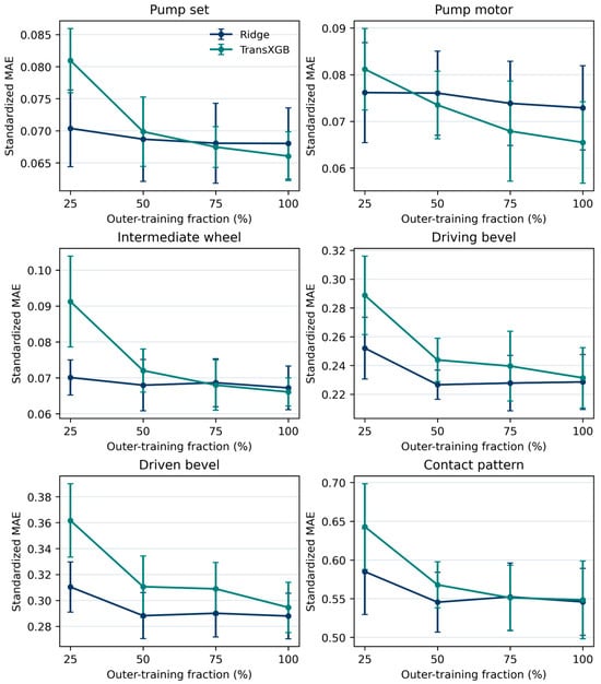
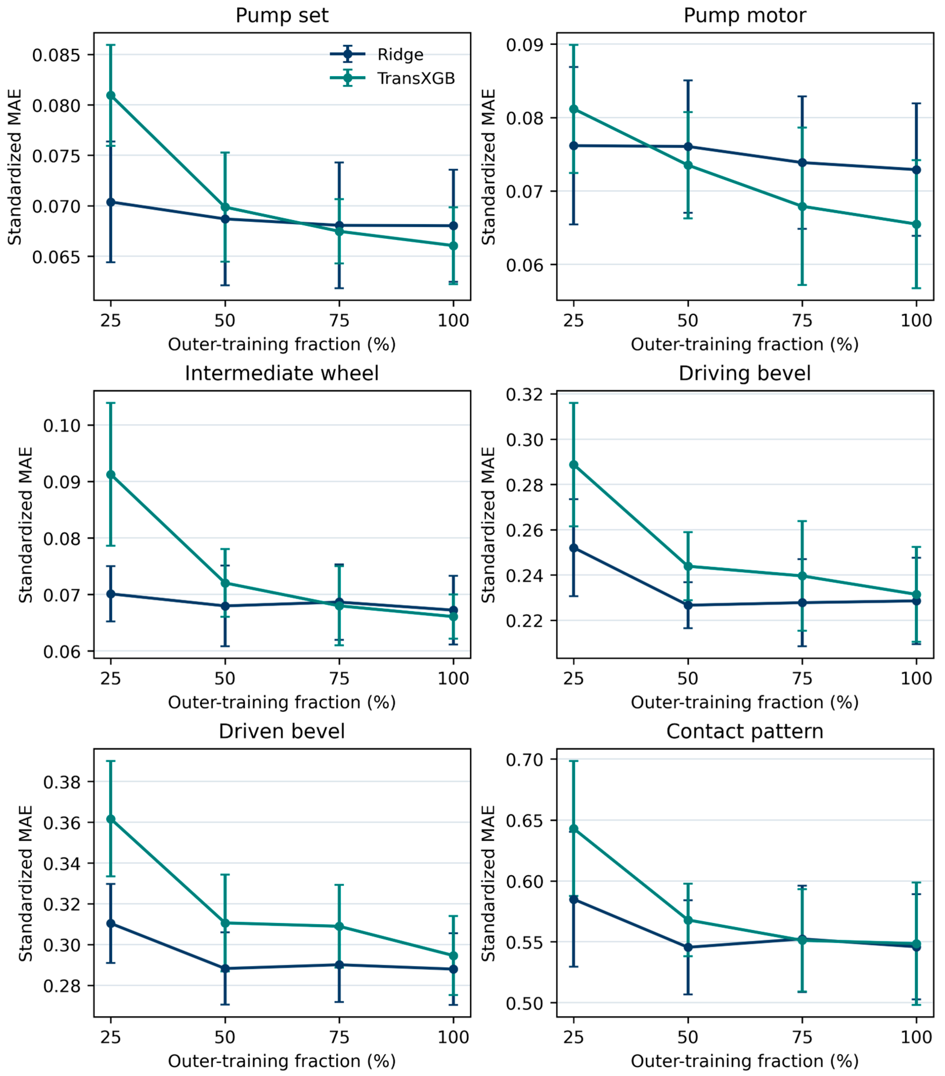
TransXGB error decreased substantially with additional rows for all tasks (Figure 8; Table 10), but only pump-set, pump-motor, and intermediate-wheel ended below Ridge at 100% training size. Contact and both bevel-shafting tasks did not show a TransXGB advantage at the available sample size. None of these curves establishes a production-data plateau because all points reuse the same generator and omit batch-level variation.
Figure 8.
Five-fold learning curves for Ridge and TransXGB using 25%, 50%, 75%, and 100% of the available outer-training rows. These curves assess convergence only within the specified synthetic mechanism.
Table 10.
Learning-curve endpoints.
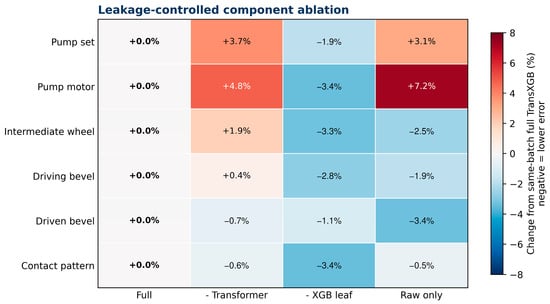
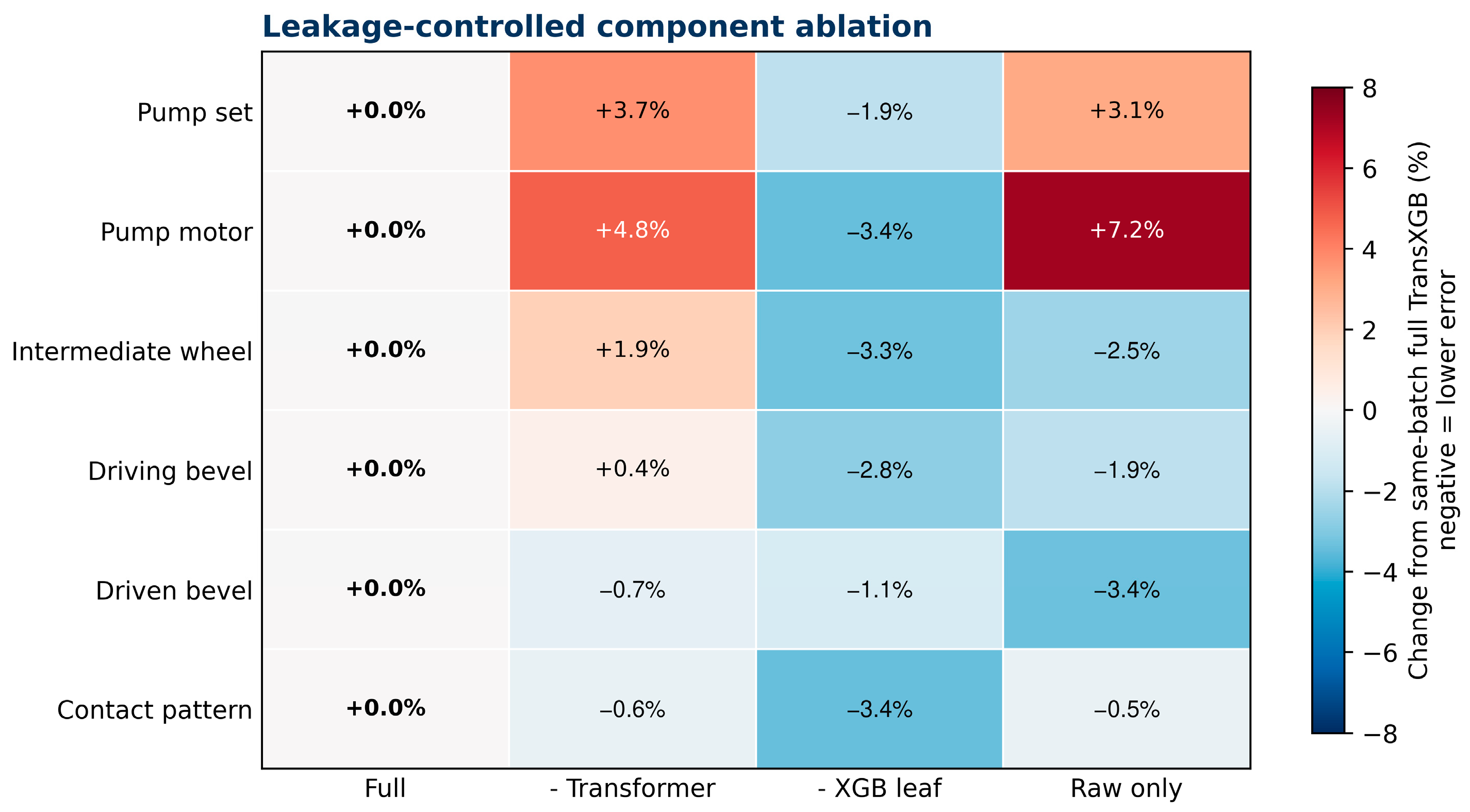
The complete same-batch rerun retained 120 fold-level evaluations (Table 11; Figure 9). Removing the XGBoost leaf branch lowered standardized MAE in all six tasks; full fusion was never best, raw-plus-Transformer was lowest in five tasks, and raw-only led the driven-bevel task. Transformer removal increased MAE by 0.00244 (3.7%) for pump-set and 0.00317 (4.8%) for pump-motor, while raw-only increased pump-motor error by 0.00478 (7.2%); each difference had the same direction in all five paired folds. The current fixed fusion therefore did not convert the leaf representation into a net gain; this supports task-selective inclusion, not the broader conclusion that tree-partition information has no value. Because the Windows rerun environment differs from the pinned primary Linux environment, the ablation remains a secondary within-batch analysis.
Table 11.
Leak-controlled component ablation (standardized MAE).
Figure 9.
Relative error change from the same-batch full TransXGB configuration in the complete five-fold component-ablation rerun. Negative values indicate lower standardized MAE. All 24 task-variant cells use retained fold-level outputs and evaluate fixed inclusion rather than the intrinsic value of tree-partition information.
3.5. Discussion in Relation to Previous Studies
Prior assembly studies modeled motion-error propagation, nonlinear spline contact, stiffness identification, and multi-sensor quality signals [1,2,3,4]. Their physical systems and measured outputs differ from this synthetic benchmark, so direct numerical comparison would be misleading. The present contribution is the leakage-controlled evaluation procedure, explicit data provenance, and publication of negative architecture findings.
The parameter-token formulation corrects the earlier 1 × 1 attention defect and yields a valid contextual representation [7]. Valid attention, however, is not evidence of better prediction. Ridge remained better on the primary aggregate, and the small S1/S2 point differences occurred in mechanisms designed to contain nonlinear terms. They define a future hypothesis rather than demonstrate model-class superiority.
The leaf branch encodes XGBoost partition structure [8,10,11], and cross-fitting prevents in-sample generation of its target-dependent features. It therefore provides a valid leakage-controlled test of complementarity with raw and Transformer features. Error was lower without the branch in all six tasks, showing that fixed fusion did not offset its redundancy and variance, not that tree partitions are intrinsically uninformative. Future work should test nested task-level gating or stronger fusion regularization. Removing the Transformer, by contrast, increased error in both pump tasks across all five paired folds. The evidence supports a simpler default configuration without claiming three-branch synergy.
Machine learning has previously been investigated for shim-gap estimation with sparse sensing [20]. Here, no signed dimensional-chain equations or measured assemblies were available, so the shafting tasks remain controlled numerical feasibility studies. A deployable workflow should place verified dimensional-chain calculations first, apply the learned model only inside a validated domain, and return uncertain or out-of-range cases to an operator.
A future operator-supervised workflow could combine signed dimensional-chain calculations with models validated on prospectively measured batches [5,6,21]. Its possible Industry 5.0 relevance is limited to traceability, human oversight, and explicit abstention [22]. The present study evaluates none of the required industrial outcomes: production accuracy, cross-batch transfer, operator performance, rework, energy use, or cycle time.
4. Limitations
First, all modeled rows are synthetic. S0 copies legacy modeling rows that project provenance identifies as normally generated, but their original target equation, random seed, and noise process are unavailable; S0 determinism or stochasticity therefore cannot be established. S1 and S2 have fully specified smooth and mixed response rules. The separate archive of 40 measured assembly records was used only for task definitions and ranges, had no row-level link to S0, and contributed no modeling rows.
Second, the underlying rows and broad architecture had been viewed during earlier development. Repeated nested CV prevents information flow across folds during the present rerun and evaluates the frozen selection procedure, but it cannot make the rows historically unseen. A prospectively collected cohort is still required for confirmatory inference.
Third, generated row identifiers do not encode production unit, component serial number, lot, operator, instrument, time, or rework. The repeated-CV variability therefore represents only row-level variation under the specified generator, not factory-level dependence.
Fourth, the three-input contact schema and the shafting schemas omit variables that a physical production study would normally examine, including material grade, heat treatment, machining route, tooth-flank geometry, surface condition, bearing preload, assembly torque, lubrication, temperature, housing deformation, inspection load, contact-measurement settings, and measurement-system uncertainty. Because no measured rows were modeled and S0’s target rule is unavailable, the present benchmark cannot estimate the contribution of any omitted physical variable or use omission as a causal explanation for the contact result.
Fifth, the contact S0 task did not outperform the training-mean predictor, and complete fold-level ablation outputs did not show a net benefit from fixed XGBoost leaf-branch inclusion. Because S0’s generating rule is unavailable, the contact failure cannot separate generator mismatch, omitted variables, noise, and model bias. These negative findings constrain the contribution to evaluation methodology rather than feature-fusion superiority.
Sixth, no signed closure equations, nominal drawing dimensions, or tolerance allocations were available for a dimensional-chain benchmark. Future work should compare model residuals with worst-case and statistical chain calculations rather than replace engineering equations with a learned proxy.
Finally, learning curves were evaluated within one generator and cannot estimate the number of measured batches needed for deployment. Future work must prospectively collect batch-identified assemblies, evaluate operator interaction, compare against signed dimensional-chain calculations, and measure production yield, rework, cycle time, energy use, and workload.
5. Conclusions
Objective 1—task and data definition. Five shafting-adjustment tasks and one contact-pattern task were defined, and every modeled row was identified as synthetic. The S1/S2 generator is fully specified; the unavailable S0 target rule and absence of measured records from the modeled dataset are now explicit.
Objective 2—architecture and leakage control. The Transformer now uses one token per parameter and d × d attention. The fusion MLP is trained only on fold-standardized raw parameters and Transformer/leaf representations that are out of fold for their feature generators; no base-model prediction is a fusion input.
Objective 3—common-protocol evaluation. The prespecified primary criterion was the six-task equal-weight combined standardized MAE. Ridge was slightly better than full TransXGB (0.211481 versus 0.211622), and matched inner selection for Ridge preserved that ordering (0.211430 versus 0.211622). The small S1/S2 point differences favoring TransXGB had descriptive intervals crossing zero and arose in deliberately nonlinear mechanisms. Removing the fixed leaf branch lowered error in all six ablations, motivating task-selective gating rather than rejection of tree partitioning itself. Conversely, Transformer removal worsened both pump tasks in every paired fold, and raw-plus-Transformer was lowest in five tasks; this is task-local evidence for simplification, not an aggregate superiority claim.
Objective 4—engineering-use boundary. The results support a reproducible evaluation of leakage-controlled feature fusion and document where the proposed components did not help. They do not establish production accuracy or transfer across batches. Prospective measurements, a verified measurement system, complete process covariates, signed dimensional-chain calculations, and a protocol fixed before data access are required for the next stage.
In summary, this methodological synthetic benchmark found Ridge best in aggregate and no net gain from fixed XGBoost leaf fusion. The leaf branch remains a valid leakage-controlled probe of tree-partition complementarity, but its inclusion should be selected rather than assumed. Raw-plus-Transformer was lowest in five tasks, and Transformer removal worsened both pump tasks in every paired fold. This motivates testing task-selective fusion without claiming an advantageous full architecture.
Supplementary Materials
The following supporting information can be downloaded at: https://www.mdpi.com/article/10.3390/machines14111288/s1. The supplementary reproducibility package contains the synthetic datasets, executable evaluation code, generation records, pooled result tables, inner-selection records, learning-curve outputs, the complete same-batch fold-level component-ablation rerun and environment record, paired task-scenario-repeat differences, the computational contract, and SHA-256 checksums.
Author Contributions
Conceptualization, Y.C., H.H., C.Y., X.W., R.L. and S.Y.; methodology, Y.C., H.H., C.Y., X.W., R.L. and S.Y.; formal analysis, Y.C., H.H., C.Y., X.W., R.L. and S.Y.; writing—review and editing, Y.C., H.H., C.Y., X.W., R.L. and S.Y. All authors have read and agreed to the published version of the manuscript.
Funding
This research was funded by the State Key Laboratory of Special Vehicle Design and Manufacturing Integration Technology, grant number GZ2025KF023.
Institutional Review Board Statement
Not applicable.
Informed Consent Statement
Not applicable.
Data Availability Statement
The third-round Supplementary Files contain the six synthetic task datasets, generator records for S1/S2, the S0 provenance limitation, pooled analysis tables, inner-selection records, the complete 120-row fold-level ablation rerun, its summary and software-environment record, and the task-scenario-repeat paired TransXGB-Ridge differences. The original full primary OOF prediction file was not retained in the archived package; the frozen entry point can regenerate it. The frozen entry point is run_nested_cv_reanalysis.py. The completed analysis used Python 3.12.13, NumPy 2.3.5, pandas 2.2.3, scikit-learn 1.8.0, PyTorch 2.8.0 + cpu, and XGBoost 3.4.1 on Linux-6.18.35-x86_64-with-glibc2.39 with 9 logical CPUs; CUDA availability was False. The master seed was 2026090901. Exact input and code hashes are stored in contract.json.
Conflicts of Interest
The authors declare no conflicts of interest.
Appendix A. Reproducibility Details
Appendix A.1. Engineering Dimensional-Chain Schematics
Figure A1.
Pump-motor input-shafting axial dimensional chain, including bearings NJ2213/NJ2214, input sleeve 042, input gear 040, oil shield 044, retaining ring 125, the housing span, and the ground sleeve-043 closure variables X − Y and Z. Colored dimensions identify closure variables and overall spans; black dimensions denote the component stack. All dimensions are in millimetres.
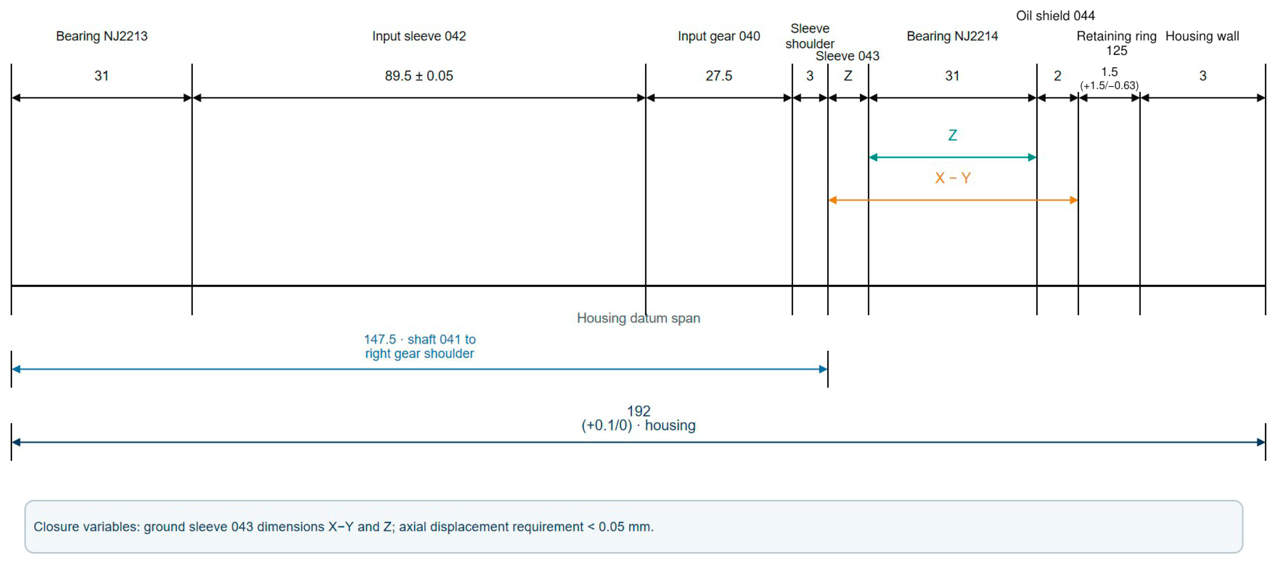
Figure A2.
Pump-set input-shafting axial dimensional chain, including retaining ring 50, adjustment shim 053 (X), round nut M52, bearings 6011, sleeve 052, and the 78 mm housing closure span. Yellow/orange identifies shim 053 (X); blue denotes the housing span. All dimensions are in millimetres.
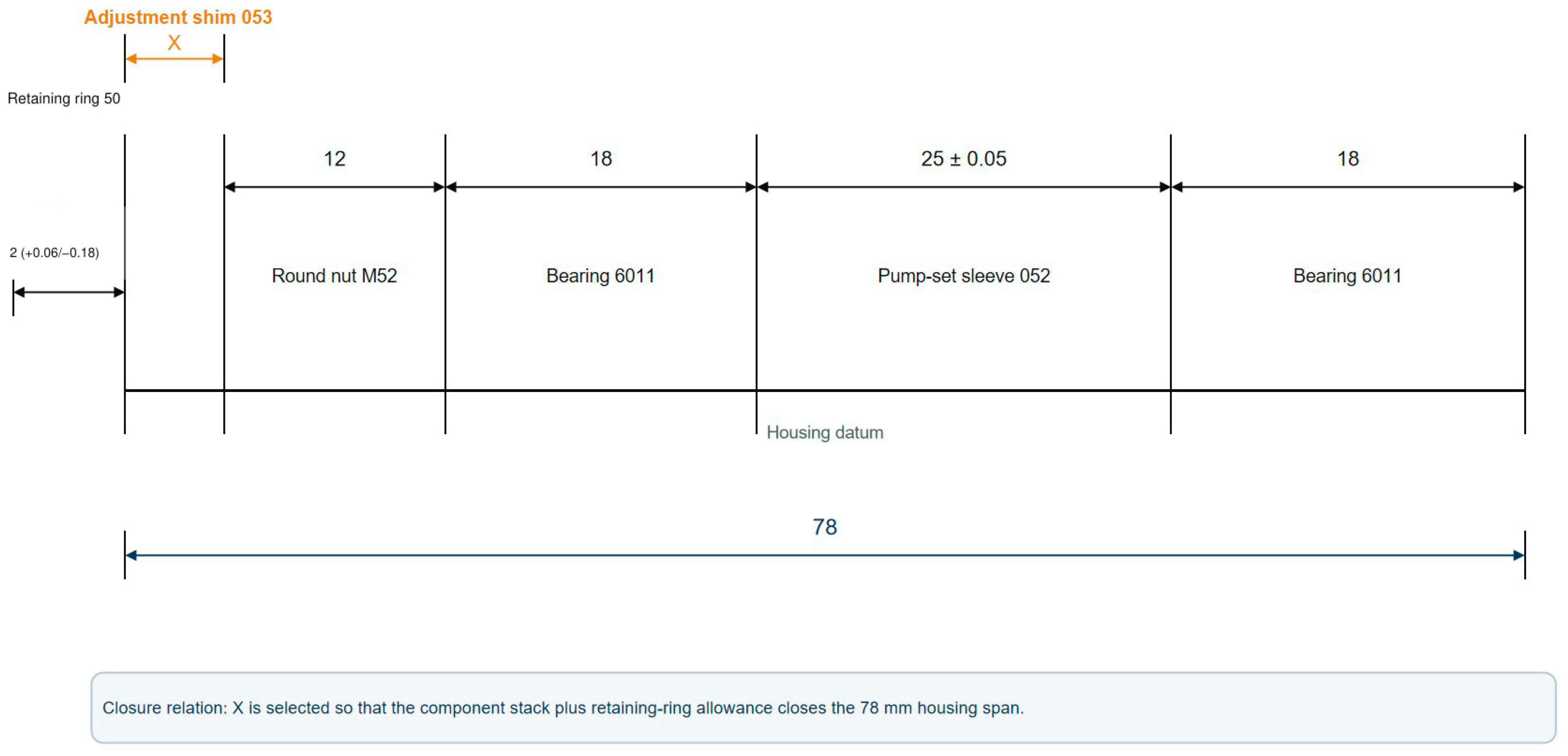
Figure A3.
Intermediate-wheel shafting axial dimensional chain, including retaining ring 40, adjustment shim 050 (X), round nut M42, bearing NUP2309, sleeve 049, gears 047/046/045, spherical roller bearing 22212, and the 221 ± 0.2 mm shaft-048 closure span. Yellow/orange identifies shim 050 (X); blue denotes the closure span. All dimensions are in millimetres.
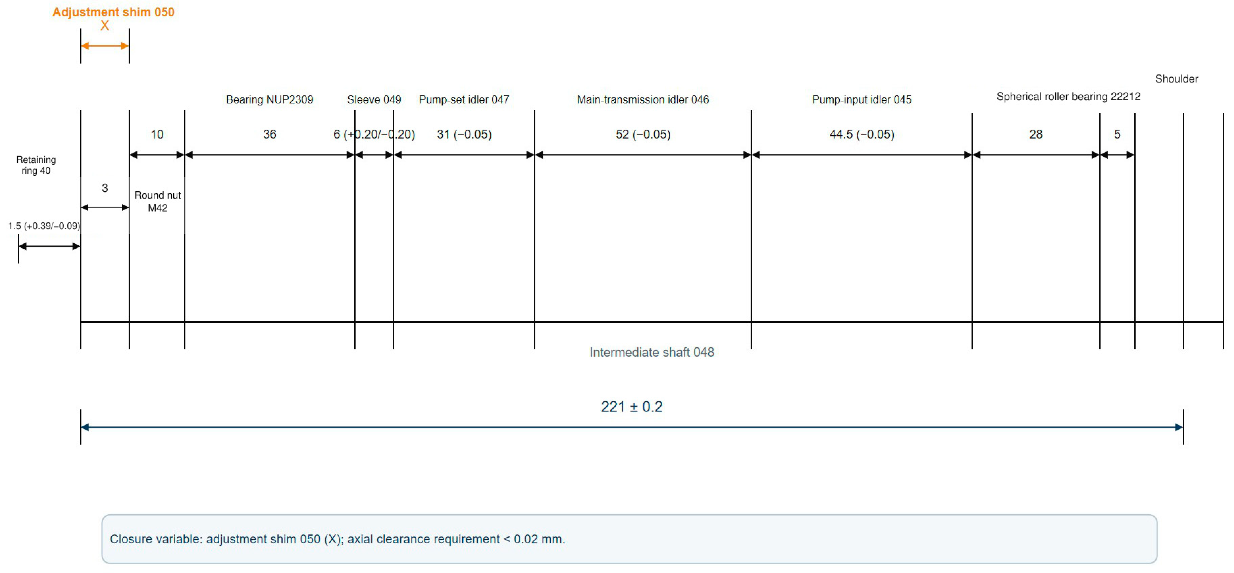
Figure A4.
Driving-bevel shafting dimensional chains: (a) shaft-side stack with bearings 32022, sleeve 020, nut M105, locking plate 007, retaining ring 100, and adjustment shims 008–011; (b) support-plate/outer-ring stack with selected sleeves 019 and 015–018 and the 0.03 mm axial-clearance requirement. Yellow/orange identifies adjustment dimensions, blue denotes closure spans, and red denotes axial clearance. All dimensions are in millimetres.
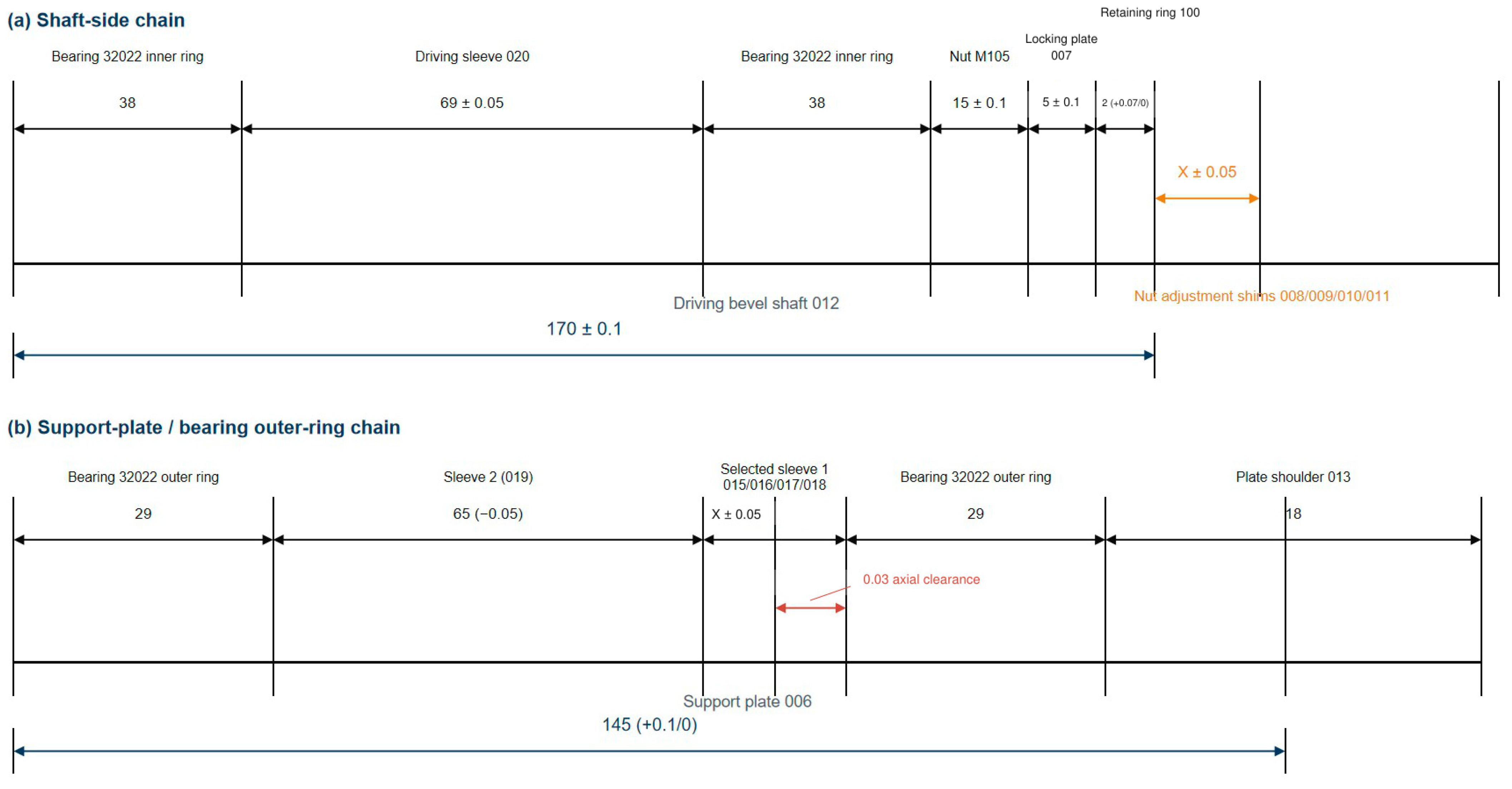
Figure A5.
Driven-bevel shafting axial dimensional chain, including bearings N313/QJ315N2MA/N220ECP, bushing 027, sleeve 033, adjustment shims 2 and 3, the retaining-ring-160 closure detail, and the 244 ± 0.5 mm driven-gear span. Blue denotes closure spans; X denotes the selected adjustment dimension. All dimensions are in millimetres.
Appendix A.2. Complete Input and Output Schema
Table A1.
Frozen feature and target columns.
Appendix A.3. Candidate Definitions and Nested Selection Frequencies
Table A2.
Frozen TransXGB candidates and inner-CV selection counts across 15 outer folds.
Appendix A.4. Run Integrity
The completed run produced 315,090 target-level predictions across ten methods, three repeats, six tasks, and 13 outputs. The archived package does not contain that full prediction file; it contains the frozen entry point and contract needed to regenerate it. The run state is COMPLETE, and the contract records SHA-256 hashes for the included data, code, and result artifacts.
Appendix A.5. Paired TransXGB-Ridge Differences by Task Scenario and Repeat
Table A3.
Standardized-MAE difference calculated as TransXGB minus Ridge.
References
- Yan, X.; Liu, Z.; Liu, W.; Zhao, Y.; Cheng, Q.; Cai, Y. A method for predicting and improving the assembly motion accuracy of linear motion systems in precision machine tools. Precis. Eng. 2026, 99, 593–606. [Google Scholar] [CrossRef] [Scilit]
- Niu, Y.; Gao, C.; Liu, Y.; Yu, H. A new assembly accuracy prediction method of spline-gear transmission systems with nonlinear contact behaviour via neural network surrogate model. CIRP J. Manuf. Sci. Technol. 2026, 67, 15–28. [Google Scholar] [CrossRef] [Scilit]
- Hu, X.; Yu, D.; Wu, T.; Nie, Y.; Hong, J.; Zhao, Q. A novel computational framework for efficient assembly accuracy prediction based on structure partition and stiffness identification. Aerosp. Sci. Technol. 2026, 177, 112521. [Google Scholar] [CrossRef] [Scilit]
- Yang, X.; Zhang, Q.; Bao, J.; Wang, X.; Wu, N.; Tao, Q.; Wu, H.; Liu, L. Predicting car-engine manufacturing quality with multi-sensor data of manufacturing assembly process. Sensors 2026, 26, 1651. [Google Scholar] [CrossRef] [Scilit] [PubMed]
- Tang, W.B.; Yan, X.; Sun, J.; Li, Y. Precision assembly error analysis of parts based on multi-constraint surface matching. Front. Mech. Eng. 2025, 10, 1519646. [Google Scholar] [CrossRef] [Scilit]
- Yang, Y.C.; Zhang, A.Q.; Liu, X.J.; Jiang, D.; Lu, Y.; Wu, B. Digital twin-driven assembly accuracy prediction method for high-performance precision assembly of complex products. Adv. Eng. Inform. 2024, 61, 102495. [Google Scholar] [CrossRef] [Scilit]
- Wang, W.; Li, H.; Liu, P.; Niu, B.; Sun, J.; Wen, B. Predicting assembly geometric errors based on Transformer neural networks. Machines 2024, 12, 161. [Google Scholar] [CrossRef] [Scilit]
- Chen, T.; Guestrin, C. XGBoost: A scalable tree boosting system. In Proceedings of the 22nd ACM SIGKDD International Conference on Knowledge Discovery and Data Mining, San Francisco, CA, USA, 13–17 August 2016; pp. 785–794. [Google Scholar]
- Vaswani, A.; Shazeer, N.; Parmar, N.; Uszkoreit, J.; Jones, L.; Gomez, A.N.; Kaiser, Ł.; Polosukhin, I. Attention is all you need. Adv. Neural Inf. Process. Syst. 2017, 30, 5998–6008. [Google Scholar]
- Friedman, J.H. Greedy function approximation: A gradient boosting machine. Ann. Stat. 2001, 29, 1189–1232. [Google Scholar] [CrossRef] [Scilit]
- Ke, G.; Meng, Q.; Finley, T.; Wang, T.; Chen, W.; Ma, W.; Ye, Q.; Liu, T.Y. LightGBM: A highly efficient gradient boosting decision tree. Adv. Neural Inf. Process. Syst. 2017, 30, 3146–3154. [Google Scholar]
- ISO 1101:2017; Geometrical Product Specifications (GPS)—Geometrical Tolerancing—Tolerances of Form, Orientation, Location and Run-Out. ISO: Geneva, Switzerland, 2017.
- ISO 22514-7:2021; Statistical Methods in Process Management—Capability and Performance—Part 7: Capability of Measurement Processes. ISO: Geneva, Switzerland, 2021.
- ISO/IEC 24029-1:2021; Artificial Intelligence (AI)—Assessment of the Robustness of Neural Networks—Part 1: Overview. ISO: Geneva, Switzerland, 2021.
- Wang, Y.; Zhang, J.; Li, Z.; Liang, R.; Zhu, R.; Ma, H. Mesh characteristic analysis of spiral bevel gear pairs considering assembly errors and tooth tip chipping faults. Appl. Sci. 2024, 14, 3227. [Google Scholar] [CrossRef] [Scilit]
- Li, H.; Qiu, L.M.; Wang, Z.L.; Zhang, S.; Tan, J.; Zhang, L. An assembly precision prediction method for customized mechanical products based on GAN-FTL. Proc. Inst. Mech. Eng. Part B J. Eng. Manuf. 2022, 236, 877–890. [Google Scholar] [CrossRef] [Scilit]
- Yang, X.; Ran, Y.; Wang, Z.C.; Mu, Z.; Zhang, G. Early prediction method for assembly precision of mechanical system and assessment of precision reliability. Int. J. Adv. Manuf. Technol. 2021, 112, 203–220. [Google Scholar] [CrossRef] [Scilit]
- Kingma, D.P.; Ba, J. Adam: A method for stochastic optimization. International Conference on Learning Representations. In Proceedings of the ICLR 2015-Conference Track Proceedings, San Diego, CA, USA, 7–9 May 2015. [Google Scholar]
- Breiman, L. Random forests. Mach. Learn. 2001, 45, 5–32. [Google Scholar] [CrossRef] [Scilit]
- Manohar, K.; Hogan, T.; Buttrick, J.; Banerjee, A.G.; Kutz, J.N.; Brunton, S.L. Predicting shim gaps in aircraft assembly with machine learning and sparse sensing. J. Manuf. Syst. 2018, 48, 87–95. [Google Scholar] [CrossRef] [Scilit]
- Schleich, B.; Wärmefjord, K.; Söderberg, R.; Wartzack, S. Geometrical variations management 4.0: Towards next generation geometry assurance. Procedia CIRP 2018, 75, 3–10. [Google Scholar] [CrossRef] [Scilit]
- European Commission; Directorate-General for Research and Innovation. Industry 5.0: Towards a Sustainable, Human-Centric and Resilient European Industry; Publications Office of the European Union: Luxembourg, 2021. [Google Scholar] [CrossRef] [PubMed]

Disclaimer/Publisher’s Note: The statements, opinions and data contained in all publications are solely those of the individual author(s) and contributor(s) and not of MDPI and/or the editor(s). MDPI and/or the editor(s) disclaim responsibility for any injury to people or property resulting from any ideas, methods, instructions or products referred to in the content. |
© 2026 by the authors. Licensee MDPI, Basel, Switzerland. This article is an open access article distributed under the terms and conditions of the Creative Commons Attribution (CC BY) license.